The crystal-fluid interfacial free energy and nucleation rate of NaCl from differentsimulation methodsJorge R. Espinosa, Carlos Vega, Chantal Valeriani, and Eduardo Sanz Citation: The Journal of Chemical Physics 142, 194709 (2015); doi: 10.1063/1.4921185 View online: http://dx.doi.org/10.1063/1.4921185 View Table of Contents: http://scitation.aip.org/content/aip/journal/jcp/142/19?ver=pdfcov Published by the AIP Publishing Articles you may be interested in Interfacial free energy of the NaCl crystal-melt interface from capillary wave fluctuations J. Chem. Phys. 142, 134706 (2015); 10.1063/1.4916398 The mold integration method for the calculation of the crystal-fluid interfacial free energy from simulations J. Chem. Phys. 141, 134709 (2014); 10.1063/1.4896621 Bcc crystal-fluid interfacial free energy in Yukawa systems J. Chem. Phys. 138, 044705 (2013); 10.1063/1.4775744 Wall-liquid and wall-crystal interfacial free energies via thermodynamic integration: A molecular dynamicssimulation study J. Chem. Phys. 137, 044707 (2012); 10.1063/1.4738500 Crystal nucleation and the solid–liquid interfacial free energy J. Chem. Phys. 136, 074510 (2012); 10.1063/1.3678214

This article is copyrighted as indicated in the article. Reuse of AIP content is subject to the terms at: http://scitation.aip.org/termsconditions. Downloaded to IP:

147.96.95.58 On: Thu, 21 May 2015 14:03:44

THE JOURNAL OF CHEMICAL PHYSICS 142, 194709 (2015)

The crystal-fluid interfacial free energy and nucleation rate of NaClfrom different simulation methods

Jorge R. Espinosa, Carlos Vega, Chantal Valeriani, and Eduardo SanzDepartamento de Química Física, Facultad de Ciencias Químicas, Universidad Complutense de Madrid,28040 Madrid, Spain

(Received 13 February 2015; accepted 4 May 2015; published online 21 May 2015)

In this work, we calculate the crystal-fluid interfacial free energy, γcf , for the Tosi-Fumi model ofNaCl using three different simulation techniques: seeding, umbrella sampling, and mold integration.The three techniques give an orientationaly averaged γcf of about 100 mJ/m2. Moreover, we observethat the shape of crystalline clusters embedded in the supercooled fluid is spherical. Using the moldintegration technique, we compute γcf for four different crystal orientations. The obtained interfacialfree energies range from 100 to 114 mJ/m2, being (100) and (111) the crystal planes with the lowestand highest γcf , respectively. Within the accuracy of our calculations, the interfacial free energy eitherdoes not depend on temperature or changes very smoothly with it. Combining the seeding techniquewith classical nucleation theory, we also estimate nucleation free energy barriers and nucleation ratesfor a wide temperature range (800-1040 K). The obtained results compare quite well with brute forcecalculations and with previous results obtained with umbrella sampling [Valeriani et al., J. Chem.Phys, 122, 194501 (2005)]. C 2015 AIP Publishing LLC. [http://dx.doi.org/10.1063/1.4921185]

I. INTRODUCTION

The crystal-fluid interfacial free energy, γcf , is a crucialparameter in crystal nucleation and growth, as well as in wett-ing phenomena.1–3 Unfortunately, it is quite difficult to mea-sure γcf experimentally.4 Typically, experimental measure-ments of the crystal nucleation rate are combined with Classi-cal Nucleation Theory (CNT)3 to estimate both the height ofthe nucleation barrier and the interfacial free energy.5–8

Computer simulations are a useful tool to estimate crystal-fluid interfacial free energies. Several simulation methods havebeen implemented for that purpose: the cleaving method,9 thecapillary fluctuation technique,10 metadynamics,11,12 tetheredMonte Carlo (MC),13 the contact angle approach,14,15 theseeding method,16–18 umbrella sampling (US),19 and themold integration (MI) technique.20 For systems like LennardJones,12,20–22 hard spheres,13,20,23–25 or water,17,18,26–28 some ofthese techniques have been used by different groups and areasonable consensus on γcf has been reached. However, thisis not the case for sodium chloride.

In 2005, two different values of γcf for the Tosi-Fumimodel29,30 of NaCl were reported: 36 mJ/m2, based onmeasures of the contact angle of a liquid drop on top ofits solid;14,31 and 99 mJ/m2, based on calculations of thenucleation free energy barrier combined with classical nucle-ation theory.32 These discrepancies were ascribed to finite sizeeffects in small crystal clusters in a combined effort by bothgroups later on in 2008.33

In our present work, we calculate γcf for the Tosi-FumiNaCl model by three different techniques, namely, moldintegration, seeding, and umbrella sampling. The MI methodconsists in calculating the work needed to reversibly inducethe formation of a crystal slab in the fluid under coexistenceconditions. The seeding technique consists in inserting large

crystalline clusters in the supercooled fluid and determiningthe temperature at which such clusters are critical. Then, CNTis used to provide estimates of the interfacial free energy. Bymeans of the US method, it is possible to compute the freeenergy needed to form crystal clusters and then CNT is usedto derive the interfacial free energy. Contrary to both umbrellasampling and seeding methods, the mold integration techniquedoes not rely on CNT and provides direct measures of γcf .

We find that the three techniques give a γcf averaged overcrystal orientations of about 100 mJ/m2. This good agreementis obtained assuming a spherical shape for the clusters both inseeding and in umbrella sampling. This assumption is justifiedby our analysis of the shape of the clusters in the seedingtechnique that confirms their spherical shape. The seedingtechnique also allows us to evaluate the dependence of γcf

with temperature and to conclude that γcf does not depend ontemperature.

The nucleation rate, i.e., the number of clusters formed perunit of time and volume, is even more relevant to characterisethe process of crystal nucleation than the interfacial freeenergy. Contrary to γcf , the nucleation rate can be directlymeasured experimentally.34–36 By means of our seedingsimulations, CNT, and calculations of the attachment rate ofparticles to the critical cluster, we estimate the nucleation rateand find a good agreement between numerical simulations andexperiments.

II. NaCl MODEL

Several model potentials have been implemented tosimulate alkali halides such as those proposed by Smith andDang,37 by Joung and Cheatham,38 or by Tosi and Fumi.29,30

We opt for the Tosi-Fumi potential, whose properties are quiteclose to those of real NaCl,29,30,39 in order to be able to compare

0021-9606/2015/142(19)/194709/12/$30.00 142, 194709-1 © 2015 AIP Publishing LLC

This article is copyrighted as indicated in the article. Reuse of AIP content is subject to the terms at: http://scitation.aip.org/termsconditions. Downloaded to IP:

147.96.95.58 On: Thu, 21 May 2015 14:03:44

194709-2 Espinosa et al. J. Chem. Phys. 142, 194709 (2015)

TABLE I. Parameters for the Tosi-Fumi NaCl,29 Ai j in kJ/mol, B in Å−1,Ci j in Å6 kJ/mol, Di j in Å8 kJ/mol, and σi j in Å.

Ai j B Ci j Di j σi j

Na–Na 25.4435 3.1546 101.1719 48.1771 2.340Na–Cl 20.3548 3.1546 674.4793 837.0770 2.755Cl–Cl 15.2661 3.1546 6985.6786 14 031.5785 3.170

with previous studies.14,31,32 Tosi-Fumi29 is a two-body andnon-polarizable potential,

U(ri j) = Ai jeB(σi j−ri j) −Ci j

r6i j

−Di j

r8i j

+qiqj

ri j, (1)

where ri j is the distance between two ions with charge qi, j. Thefirst term is the Born-Mayer repulsive term, −Ci j

r6i j

and −Di j

r8i j

are the van der Waals attractive interaction terms, and the lastone corresponds to the Coulomb interaction. The parametersAi j, B, Ci j, Di j, and σi j are given in Table I.

In this work, we have truncated the non-Coulomb part ofthe potential at rc = 14 Å and added long range tail correctionsto the energy (when simulating the system with MC andMolecular Dynamics (MD)) and pressure (in MD). We haveused Ewald sums (in MC) to deal with Coulomb interactions,truncating the real part of the sums at the same cut-off. ForMD calculations, we have used PME (Particle-Mesh Ewaldmethod)40 truncating at the same cut-off.

III. SIMULATION DETAILS

We have used the GROMACS 4.5.5 package41,42 toperform molecular dynamics simulations in the N pTensemble. The Tosi-Fumi NaCl potential has been imple-mented in GROMACS in a tabulated form. The time step forthe velocity-Verlet algorithm was set to 0.002 ps and a velocity-rescale thermostat with a relaxation time of 0.5 ps was used tokeep constant the selected temperature.43 All our simulationsare carried out at 1 bar using the Parrinello-Rahman barostat44

with a relaxation time of 0.5 ps.

IV. MOLD INTEGRATION METHOD

This methodology has been recently proposed by Es-pinosa et al.20 and allows to calculate the crystal-fluidinterfacial free energy for a flat interface (at coexistence).The method has been validated with the calculation of γcf forhard spheres and Lennard-Jones.20

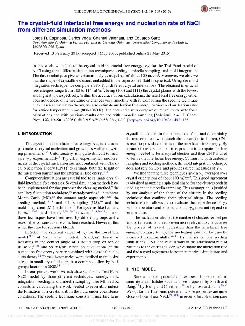
The basic idea of this methodology is to reversibly inducethe formation of a thin crystalline slab in the fluid with theaid of a mold of potential energy wells placed in the sites ofa lattice plane. By switching on a square-well-like interactionbetween the wells and the fluid particles, the latter remainconfined in the mold inducing the appearance of a thin crystalslab as sketched in Fig. 1.45 In Fig. 1(a), the mold (orange andgray spheres) is switched off and the fluid (small particles)does not feel its presence. In (b), the mold is switched onand each well is filled with a fluid particle, which creates acrystal slab around the mold. The work needed to go from (a)

FIG. 1. Top: Snapshot of a sodium chloride fluid at coexistence (green andblack ions). Bottom: Snapshot of a fluid with a thin crystal slab at coexistenceconditions. The diameter of the ions has been reduced to 1/4 of its originalsize. The mold that induces the formation of the crystal slab is conformed bya set of potential energy wells (in orange the ones for sodium ions and in greythe ones for chloride ions) whose positions are given by the lattice sites ofthe selected crystal plane, (100) in this case, at coexistence conditions. Theinteraction between the mold and the ions is switched off in (a) and on in (b).

to (b) is related to the work required to create two crystal-fluidinterfaces.20

The only difference from the present work and Ref. 20in terms of methodology is that here we use two differenttypes of wells that selectively attract either Na+ or Cl− ions.(The systems studied in Ref. 20 were mono-component, soevery well interacted with every particle.) In Sec. IV A, wedescribe how the interfacial free energy is calculated for the

This article is copyrighted as indicated in the article. Reuse of AIP content is subject to the terms at: http://scitation.aip.org/termsconditions. Downloaded to IP:

147.96.95.58 On: Thu, 21 May 2015 14:03:44

194709-3 Espinosa et al. J. Chem. Phys. 142, 194709 (2015)

(100) plane of NaCl with the MI method and give the resultsfor other orientations.

A. Calculation of γcf with the MI method

In this section, we report the calculation of γcf for fourdifferent crystal orientations using the MI method. We willstart with explaining in more detail the calculations for the100 plane and then give the results for all other orientations.

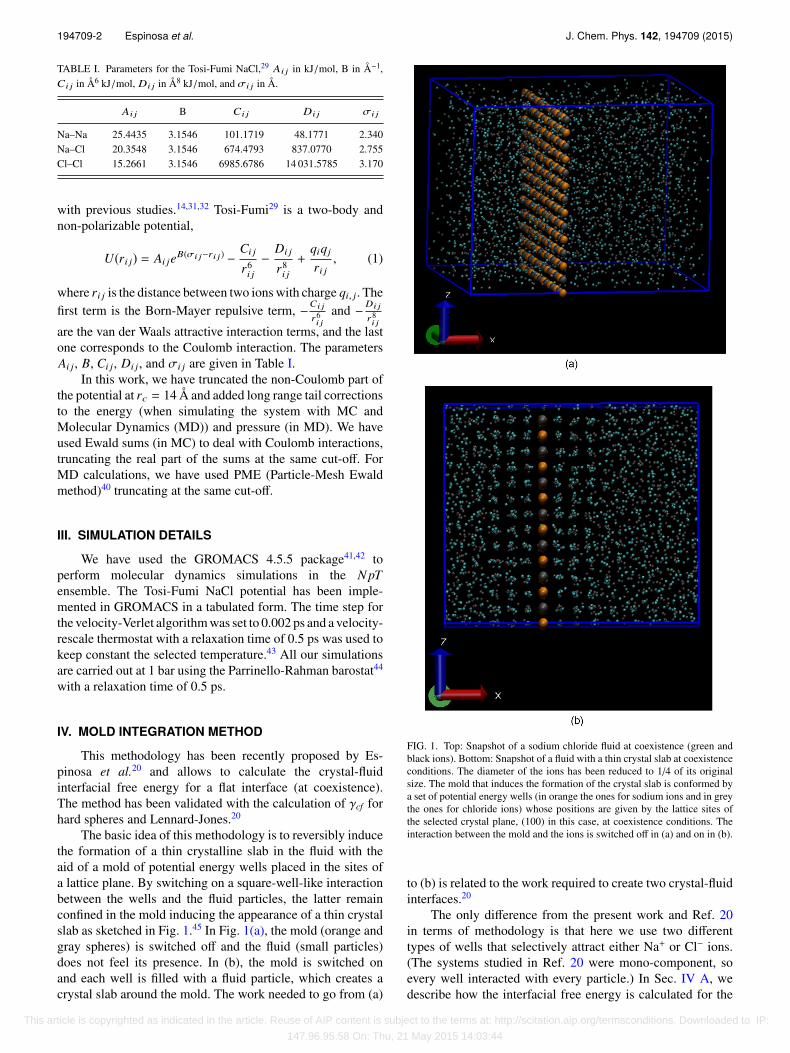
The first step is obtaining the mold coordinates and afluid configuration at coexistence conditions. The dimensionsof the mold have to be coherent with the unit cell parametersat coexistence conditions. In Figs. 1 and 2, we show arepresentation of the molds used to induce the appearanceof different crystal-fluid interfaces.

The mold for the (100) orientation has 196 wells, half forsodium and half for chloride ions. The fluid consists of 2744ions equilibrated at coexistence conditions. The simulationbox where the fluid is equilibrated is prepared in such way thatthe area of one of its sides coincides with that of the mold (seeFig. 1(a)). This side is kept fixed and to maintain the pressureconstant, variations of the volume are made through changesin the direction perpendicular to it, which in our case is the xdirection (we refer to this type of simulations as N pxT46). Themold is kept fixed throughout the simulation.

Once a fluid-mold configuration is prepared, we needto find the potential well radius that gives the correct valuefor γcf , row (the work needed to fill the mold depends on thewell radius and there is only one radius for which the correctinterfacial free energy is obtained20). To find row, we run, for

FIG. 2. Molds used to induce the formation of crystal slabs for the differentcrystal orientations.

different values rw of the well radius, several N pxT trajectoriesstarting from a fluid configuration where we switch on themold at the beginning of the simulation. In the present paper,we launch 8 trajectories of 1 ns for each rw. We set the depthof the square-well-like interaction between wells and particlesto ϵm = 7.5 kBT . This ensures that the mold is permanentlyfilled (195.6 out of 196 wells are filled on average). Alongeach trajectory, we monitor a parameter that accounts for theglobal degree of crystallinity, ξ,

ξ =ρ − ρ f

ρs − ρ f, (2)

where ρ is the actual density of the system, and ρ f and ρs arethe coexistence densities of the fluid and the solid, respectively.Therefore, ξ fluctuates around 0 when the whole system is fluidand around 1 when is crystalline. As a crystal slab grows in thefluid, ξ takes intermediate values. This is just a simple way toquantify the crystallinity degree, but one can also use a methodbased on counting the number of ions in the largest cluster ofsolid-like ions, using the same local order parameter as the onewe use in the “seeding” technique (see below). By means ofthe trajectories launched for each rw, we obtain a probabilitydistribution P(ξ) needed to estimate the free energy profileassociated to the order parameter ξ,

G(ξ)/(kBT) = − ln P(ξ) + constant. (3)

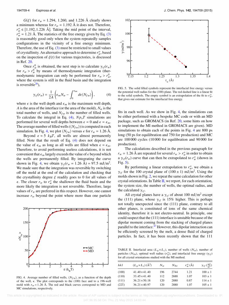
The constant is not known, but we are interested in whether thefree energy profile shows a minimum or not. As discussed inRef. 20, if rw is too large, the system is in the free energy basincorresponding to the fluid, as the mold is not able to induce theformation of a stable crystal slab. If, on the contrary, rw is toosmall, the mold provides more energy than that required forthe formation of the crystal slab and the G(ξ) profile does notshow a basin (a minimum) corresponding to the fluid phase.Accordingly, the free energy profile where the minimum firstdisappears gives row. In Fig. 3, we represent the free energyprofiles for four different values of rw.

FIG. 3. Free energy profile as a function of the crystallinity degree, ξ, for the100 plane and for different well radii as indicated in the legend (in Å). In orderto compare all curves in the same scale, we have shifted each minimum to thework needed to fill the mold for the corresponding well radius (calculatedvia thermodynamic integration). For the case where the minimum is absent(black curve), we have shifted the plateau to the work needed to fill a mold ofwells with rw = r

ow, given by the dashed horizontal line.

This article is copyrighted as indicated in the article. Reuse of AIP content is subject to the terms at: http://scitation.aip.org/termsconditions. Downloaded to IP:

147.96.95.58 On: Thu, 21 May 2015 14:03:44

194709-4 Espinosa et al. J. Chem. Phys. 142, 194709 (2015)

G(ξ) for rw = 1.294, 1.260, and 1.226 Å clearly showsa minimum whereas for rw = 1.192 Å it does not. Therefore,row ∈ [1.192,1.226 Å]. Taking the mid point of the interval,row = 1.21 Å. The statistics of the free energy given by Eq. (3)is reasonably good only when the system repeatedly samplesconfigurations in the vicinity of a free energy minimum.Therefore, the use of Eq. (3) must be restricted to small valuesof crystallinity. An alternative approach to determine row, basedon the inspection of ξ(t) for various trajectories, is discussedin Ref. 20.

Once r0w is obtained, the next step is to calculate γcf (rw)

for rw > r0w by means of thermodynamic integration (ther-

modynamic integration can only be performed for rw > r0w,

where the system is still in the fluid basin and the integrationis reversible20),

γcf (rw) = 12A

(ϵmNw −

ϵm

0dϵ⟨Nf w⟩

), (4)

where ϵ is the well depth and ϵm is the maximum well depth,A is the area of the interface (or the area of the mold), Nw is thetotal number of wells, and Nf w is the number of filled wells.To calculate the integral in Eq. (4), N pxT simulations areperformed for several well depths between ϵ = 0 and ϵ = ϵm.The average number of filled wells (⟨Nf w⟩) is computed in eachsimulation. In Fig. 4, we plot ⟨Nf w⟩ versus ϵ for rw = 1.26 Å.

Beyond ϵ ≈ 5 kBT , all wells are almost permanentlyfilled. Note that the result of Eq. (4) does not depend onthe value of ϵm as long as all wells are filled when ϵ = ϵm.Therefore, to avoid performing useless calculations, it is notconvenient that ϵm largely exceeds the value of ϵ beyond whichthe wells are permanently filled. By integrating the curveshown in Fig. 4, we obtain γcf (rw = 1.26 Å) = 97.5 mJ/m2.We made sure that the integration was reversible by switchingoff the mold at the end of the calculation and checking thatthe crystallinity degree ξ readily goes to 0 for all values ofϵ . The closer rw to row the shallower the fluid basin and themore likely the integration is not reversible. Therefore, largevalues of rw are preferred in this respect. However, one cannotincrease rw beyond the point where more than one particle

FIG. 4. Average number of filled wells, ⟨N f w⟩, as a function of the depthof the well, ϵ. The plot corresponds to the (100) face and to a 196-wellmold with rw = 1.26 Å. The red and black curves correspond to MD andMC simulations, respectively.

FIG. 5. The solid filled symbols represent the interfacial free energy versusthe potential well radius for the (100) plane. The red dashed line is a linear fitto the solid symbols. The empty symbol is an extrapolation of the fit to row,that gives our estimate for the interfacial free energy.

fits in each well. As we show in Fig. 4, the simulations canbe either performed with a bespoke MC code or with an MDpackage, such as GROMACS (in Ref. 20, some hints on howto implement the MI method in GROMACS are given). MDsimulations to obtain each of the points in Fig. 4 are 800 pslong (50 ps for equilibration and 750 for production) and MCare 100 000 cycles (10 000 for equilibration and 90 000 forproduction).

The calculations described in the previous paragraph forrw = 1.26 Å are repeated for several rw > row in order to obtaina γcf (rw) curve that can then be extrapolated to row (shown inFig. 5).

By performing a linear extrapolation to row, we obtain aγcf for the 100 crystal plane of (100 ± 1) mJ/m2. Using themolds shown in Fig. 2, we repeat the same calculation for othercrystal orientations. In Table II, we report, for each orientation,the system size, the number of wells, the optimal radius, andthe calculated γcf .

All crystal planes have a γcf of about 100 mJ/m2 exceptthe (111) plane, whose γcf is 15% higher. This is perhapsnot totally unexpected since the (111) plane, contrary to allother planes, is constituted of ions of the same chemicalidentity, therefore it is not electro-neutral. In principle, onecould suspect that the (111) interface is unstable because of thedipolar moment coming from the stacking of charged planesparallel to the interface.47 However, this dipolar interaction canbe efficiently screened by the melt, a dense fluid of chargedparticles. In fact, it has been recently shown that the 111

TABLE II. Interfacial area (L y×Lz), number of wells (Nw), number ofparticles (NTot), optimal well radius (row), and interfacial free energy (γcf )for all crystal orientations studied with the MI method.

hkl (L y×Lz) (Å2) Nw NTot row (Å) γcf (mJm2 )

(100) 41.40×41.40 196 2744 1.21 100 ± 1(110) 33.45×41.40 112 2688 1.07 103 ± 1(111) 36.21×50.18 120 2880 0.87 114 ± 1(221̄) 36.21×40.97 120 2880 1.07 105 ± 1

This article is copyrighted as indicated in the article. Reuse of AIP content is subject to the terms at: http://scitation.aip.org/termsconditions. Downloaded to IP:

147.96.95.58 On: Thu, 21 May 2015 14:03:44

194709-5 Espinosa et al. J. Chem. Phys. 142, 194709 (2015)

crystal-melt interface of NaCl is rough and shows no signs ofbeing unstable or undergoing surface reconstruction.48

V. SEEDING

A. The seeding technique

This technique has been first proposed by Bai and Li16,49

for the calculation of the crystal-fluid interfacial free energy ofthe Lennard-Jones system. Later on, it was used to determineγcf for clathrates17 and for several water models.18,28 In brief,it consists in inserting a crystalline cluster in a supercooledfluid and performing simulations at several temperatures whilemonitoring the size of the cluster. If the chosen temperatureis below the temperature at which the cluster is critical, thecluster will grow, whereas if it is above, the cluster will melt.So the temperature at which the cluster is critical is enclosedin between the highest temperature at which the cluster growsand the lowest at which it melts. This approach is similar tothe one used by Pereyra et al.50 to determine the temperatureat which a cylindrical crystalline slab of ice melts or grows.

Once the temperature at which the cluster is critical isknown, the seeding approach makes use of CNT to obtainestimates of the interfacial free energy. According to CNT,3

the free energy required for the formation of a crystallinecluster in the supercooled fluid is

∆G(N) = −N |∆µ| + Aγcf , (5)

where ∆µ is the chemical potential difference between thecrystal and the supercooled fluid, N is the number of particlesin the crystal cluster, and A is the cluster’s surface area.Assuming that the crystalline cluster has a spherical shape,the value of N that maximizes ∆G (Nc) is given by

Nc =32πγ3

cf

3ρ2s |∆µ|3

, (6)

where ρs is the density of the solid phase. This equationallows to estimate γcf . There are two ways of calculating∆µ. The first one is by means of thermodynamic integrationfrom the coexistence temperature, where ∆µ = 0. The other isby approximating ∆µ by ∆Hm(1 − T/Tm), where ∆Hm is themelting enthalpy and Tm is the melting temperature. We havechecked that the approximation works well and gives the sameresult as the rigorous thermodynamic integration.

Apart from obtaining estimates of γcf via Eq. (6), onecan estimate the nucleation free energy barrier (∆Gc) and thenucleation rate (J) with CNT. The free energy barrier fornucleation is given by

∆Gc =Nc

2|∆µ|. (7)

Following the approach described by Auer and Frenkel,3,19,51

the nucleation rate J can be obtained from the expression,

J = ρ f Z f + exp(−∆Gc/(kBTc)), (8)

where the product ρ f Z f + defines the kinetic prefactor, κp,where f + the attachment rate of particles to the critical cluster,ρ f the fluid density, and Z the Zeldovich factor.3 The CNT

form of the Zeldovich factor is

Z =(|∆G′′|Nc/(2πkBTc)) =

|∆µ|/(6πkBTcNc) (9)

so that Z can be computed once the size of the criticalcluster, Nc, the temperature at which it is critical, Tc, andthe chemical potential difference between the solid and theliquid are known. According to Refs. 19, 32, and 51, f + canbe computed as a diffusion coefficient of the cluster size at thetop of the barrier (which requires launching about 10 runs atthe temperature at which the cluster is critical),

f + =⟨(N(t) − Nc)2⟩

2t. (10)

Alternatively, f + can be approximated in a way that does notrequire running simulations of the critical cluster.3 Accordingto Ref. 3, since the attachment rate f + is related to the timerequired for a particle to attach to the crystal cluster, it can beestimated as

f + =24D(Nc)2/3

λ2 , (11)

where λ2/D is the time needed for a molecule to diffuse thetypical distance (λ) required to attach to the cluster and D isthe diffusion coefficient of the supercooled liquid.

The seeding technique can be particularly useful at lowand moderate supercooling, where estimating the criticalcluster size, the free-energy barrier height and the rate bymore rigorous numerical techniques would be very expensive(from a computational point of view).

B. Approximations in the seeding approach

The seeding technique is an approximate approach tocalculate γcf . First of all, it relies on the validity of CNT. Next,the inserted clusters have a defined shape. The expressionsabove for the CNT correspond to the assumption that theclusters are spherical. We will discuss later on that this isactually a good approximation for NaCl. The interfacial freeenergy thus obtained corresponds to an average over allpossible crystal orientations, so the technique does not provideinformation about the anisotropy of γcf with the orientation ofthe crystal. Finally, the method heavily relies on the way thenumber of particles in the cluster (Nc) is determined. This istypically evaluated with the aid of local bond-order parameter,which is able to discriminate between liquid-like and solid-like particles.52 Therefore, Nc depends on the specific choiceof the order parameter. Of course, reasonable choices oforder parameter give similar values for Nc, but differencesof about 30% in the number of particles can be found betweendifferent order parameters. According to Eq. (6), a 30% errorin Nc results in an uncertainty of 10% in γcf . Therefore, theambiguity in the determination of Nc substantially affectsthe accuracy with which γcf is determined via the seedingtechnique.

In this work, we use the same order parameter as in Ref. 32to measure Nc. In Ref. 32, the order parameter was tuned sothat the percentage of particles wrongly labelled as liquid-likein the bulk solid was the same as that of particles wronglylabelled as solid-like in the bulk liquid. The same criterion was

This article is copyrighted as indicated in the article. Reuse of AIP content is subject to the terms at: http://scitation.aip.org/termsconditions. Downloaded to IP:

147.96.95.58 On: Thu, 21 May 2015 14:03:44

194709-6 Espinosa et al. J. Chem. Phys. 142, 194709 (2015)

FIG. 6. (a) Snapshot of a solid cluster as detected by the local order parameterused in this work (same as in Ref. 32). (b) Same cluster as in (a) but with anextra layer of particles attached to it. (c) Same cluster as in (a) but with twoextra layers of particles attached to it. (d) Same cluster as in (a) but with threeextra layers of particles attached to it. The crystalline character of the clusterfades as extra layers are added.

used to tune the order parameter when studying the ice-waterinterface and this led to reasonable values for γcf .18,28

We can also check if our choice of the order parameter isreasonable by visually inspecting the clusters.

In Fig. 6(a), we show the top view of a cluster as detectedby our order parameter. The crystalline features of the clustercan be clearly appreciated. In Figs. 6(b)–6(d), we show thesnapshots resulting from adding 1, 2, and 3 extra layersof particles to the cluster originally detected by our orderparameter. These extra layers do not perfectly fit on top ofthe underlying solid lattice. Therefore, the order parameteremployed seems to be a good one because it does not adda fluid-like layer to the cluster (neither removes a solid-likelayer from it).

C. Setup for the seeding technique

To prepare the initial configuration, we insert a crystallinecluster in the supercooled fluid and remove the fluid moleculesthat overlap with the cluster. Then, the fluid-crystal interfaceis equilibrated for 8 ps keeping the positions of the ionsof the inserted cluster fixed. In this way, the cluster doesnot loose particles and the interface is equilibrated by theattachment of new particles to the cluster. Then, the constraintis released and the system is further equilibrated for 8 psuntil N varies smoothly with time. Following equilibration,we launch trajectories at different temperatures to find thetemperature at which the equilibrated cluster is critical.

In Fig. 7, we show the evolution of N with timeduring equilibration and during production, when trajectoriesare launched at different temperatures from the equilibratedcluster. The equilibration is typically performed at lowtemperatures (925 K in this particular case) to avoid the clusterloosing particles during the second stage of equilibration.

A list of all cluster sizes after equilibration is given inTable III.

FIG. 7. Number of particles in the cluster (N ) versus time. During thefirst stage of equilibration (8 ps, blue curve) the cluster is kept frozen andit grows as the interface equilibrates. In the second stage (red curve) theconstraint is released and the system is equilibrated for another 8 ps. Thesetwo equilibration runs are performed at 925 K. Finally, several simulationsstarting from the configuration of the equilibrated cluster are run at differenttemperatures to locate the temperature at which such cluster is critical.

In each system, the total number of ions is approximately20 times larger than the inserted cluster to avoid interactionsbetween the cluster and its periodic images. The total numberof ions, NTot, for each system (considering the solid clusterand the supercooled fluid) is also given in Table III: in orderto be able to simulate such large systems, we had to recur tosupercomputing facilities.

D. Cluster shape

The CNT expressions given above correspond to theassumption that the critical cluster adopts a spherical shape.In principle, this is a reasonable assumption because a sphereis the shape with the lowest surface area. However, in Ref. 32,it was suggested that the cluster could be cubic rather thanspherical. This is a plausible possibility for the cluster’s shape,given that NaCl has a cubic unit cell. To investigate if the shapeof the cluster is spherical or cubic, we equilibrate both a cubiccluster and a spherical cluster and compare the shape of theresulting clusters. In Fig. 8(a), we show a snapshot of bothclusters just after being inserted and in Fig. 8(b) after theequilibration of the interface.

In Fig. 8(b), 60 independent equilibrated clusters aresuperimposed (with the same orientation) in order to get a

TABLE III. Number of ions in the critical cluster (Nc), total number ofions in the system (NTot), temperature at which the cluster is found to becritical (Tc [K]), density of the solid at that temperature (ρs [g/cm3]) and theinterfacial free energy from Eq. (6) in mJ/m2.

Nc NTot Tc ρs γcf

284 21 724 857.5 1.95 1131 152 46 522 962.5 1.92 972 322 46 396 980.0 1.91 1048 084 110 248 1007.5 1.90 11411 164 194 920 1022.5 1.89 102

This article is copyrighted as indicated in the article. Reuse of AIP content is subject to the terms at: http://scitation.aip.org/termsconditions. Downloaded to IP:

147.96.95.58 On: Thu, 21 May 2015 14:03:44

194709-7 Espinosa et al. J. Chem. Phys. 142, 194709 (2015)

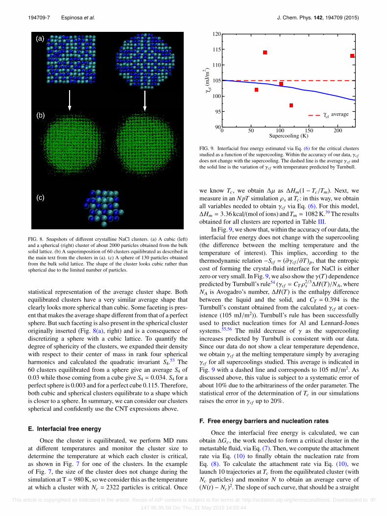
FIG. 8. Snapshots of different crystalline NaCl clusters. (a) A cubic (left)and a spherical (right) cluster of about 2000 particles obtained from the bulksolid lattice. (b) A superimposition of 60 clusters equilibrated as described inthe main text from the clusters in (a). (c) A sphere of 130 particles obtainedfrom the bulk solid lattice. The shape of the cluster looks cubic rather thanspherical due to the limited number of particles.

statistical representation of the average cluster shape. Bothequilibrated clusters have a very similar average shape thatclearly looks more spherical than cubic. Some faceting is pres-ent that makes the average shape different from that of a perfectsphere. But such faceting is also present in the spherical clusteroriginally inserted (Fig. 8(a), right) and is a consequence ofdiscretizing a sphere with a cubic lattice. To quantify thedegree of sphericity of the clusters, we expanded their densitywith respect to their center of mass in rank four sphericalharmonics and calculated the quadratic invariant S4.53 The60 clusters equilibrated from a sphere give an average S4 of0.03 while those coming from a cube give S4 = 0.034. S4 for aperfect sphere is 0.003 and for a perfect cube 0.115. Therefore,both cubic and spherical clusters equilibrate to a shape whichis closer to a sphere. In summary, we can consider our clustersspherical and confidently use the CNT expressions above.

E. Interfacial free energy

Once the cluster is equilibrated, we perform MD runsat different temperatures and monitor the cluster size todetermine the temperature at which each cluster is critical,as shown in Fig. 7 for one of the clusters. In the exampleof Fig. 7, the size of the cluster does not change during thesimulation at T = 980 K, so we consider this as the temperatureat which a cluster with Nc = 2322 particles is critical. Once

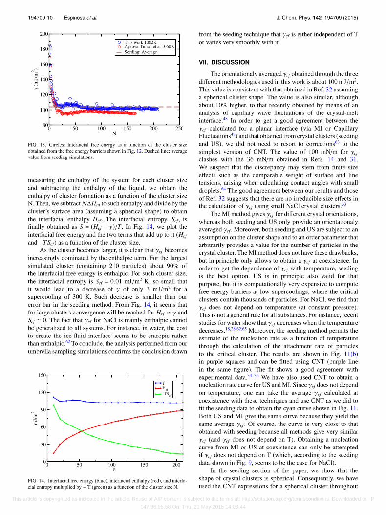
FIG. 9. Interfacial free energy estimated via Eq. (6) for the critical clustersstudied as a function of the supercooling. Within the accuracy of our data, γcfdoes not change with the supercooling. The dashed line is the average γcf andthe solid line is the variation of γcf with temperature predicted by Turnbull.

we know Tc, we obtain ∆µ as ∆Hm(1 − Tc/Tm). Next, wemeasure in an N pT simulation ρs at Tc: in this way, we obtainall variables needed to obtain γcf via Eq. (6). For this model,∆Hm = 3.36 kcal/(mol of ions) and Tm = 1082 K.39 The resultsobtained for all clusters are reported in Table III.

In Fig. 9, we show that, within the accuracy of our data, theinterfacial free energy does not change with the supercooling(the difference between the melting temperature and thetemperature of interest). This implies, according to thethermodynamic relation −Scf = (∂γcf/∂T)p, that the entropiccost of forming the crystal-fluid interface for NaCl is eitherzero or very small. In Fig. 9, we also show the γ(T) dependencepredicted by Turnbull’s rule54 (γcf = CT ρ

2/3s ∆H(T)/NA, where

NA is Avogadro’s number, ∆H(T) is the enthalpy differencebetween the liquid and the solid, and CT = 0.394 is theTurnbull’s constant obtained from the calculated γcf at coex-istence (105 mJ/m2)). Turnbull’s rule has been successfullyused to predict nucleation times for Al and Lennard-Jonessystems.55,56 The mild decrease of γ as the supercoolingincreases predicted by Turnbull is consistent with our data.Since our data do not show a clear temperature dependence,we obtain γcf at the melting temperature simply by averagingγcf for all supercoolings studied. This average is indicated inFig. 9 with a dashed line and corresponds to 105 mJ/m2. Asdiscussed above, this value is subject to a systematic error ofabout 10% due to the arbitrariness of the order parameter. Thestatistical error of the determination of Tc in our simulationsraises the error in γcf up to 20%.

F. Free energy barriers and nucleation rates

Once the interfacial free energy is calculated, we canobtain ∆Gc, the work needed to form a critical cluster in themetastable fluid, via Eq. (7). Then, we compute the attachmentrate via Eq. (10) to finally obtain the nucleation rate fromEq. (8). To calculate the attachment rate via Eq. (10), welaunch 10 trajectories at Tc from the equilibrated cluster (withNc particles) and monitor N to obtain an average curve of(N(t) − Nc)2. The slope of such curve, that should be a straight

This article is copyrighted as indicated in the article. Reuse of AIP content is subject to the terms at: http://scitation.aip.org/termsconditions. Downloaded to IP:

147.96.95.58 On: Thu, 21 May 2015 14:03:44

194709-8 Espinosa et al. J. Chem. Phys. 142, 194709 (2015)

(a)

(b)

FIG. 10. (a) N versus time for 10 trajectories launched at the temperatureat which the cluster is critical (T = 1007.5 K). (b) ⟨(N −Nc)2⟩ versus time,whose slope is related to the attachment rate by Eq. (10).

line in the regime in which the cluster diffuses on top of thebarrier, is related to the attachment rate by Eq. (10). The timeevolution of N in the ten trajectories and the resulting average(N(t) − Nc)2 curve are shown in Fig. 10.

Note that, since the simulations are performed at Tc, insome of the trajectories the cluster grows, in others it shrinks,and in others it does not change its size. In Table IV, we reportour results for all quantities needed for the calculation of thenucleation barrier and the nucleation rate.

TABLE IV. Studied cluster sizes (Nc), temperature at which the clustersare found to be critical (Tc) in K and the corresponding values for theattachment rate ( f +), in s−1; the Zeldovich factor (Z ); the kinetic prefactor(κp = ρ f Z f +), in m−3 s−1; the height of the nucleation free energy barrier(∆Gc), in kBT ; the log10 of the nucleation rate (J ) in m−3 s−1; and theconstant λ in Å.

Nc Tc f +/1014 Z/10−3 κp/1040 ∆Gc log10J λ

284 857.5 1.0 17 2.3 57 16 0.31 152 962.5 4.2 5.9 3.1 111 −8 1.72 322 980.0 6.0 3.8 3.2 188 −41 2.08 084 1007.5 10 1.7 3.4 465 −162 1.111 164 1022.5 20 1.3 3.5 506 −180 3.4

(a)

(b)

FIG. 11. Free energy barrier height, (a), and nucleation rate, (b), as a functionof the supercooling. Purple squares correspond to our seeding data, red circlesare results from Ref. 32, the blue triangle is an experimental data fromRefs. 34–36, and the black squares are our calculations of the nucleation ratefrom brute force MD calculations. The curves are fits based on the seedingdata (purple) and on the estimates of γcf at coexistence by means of the MImethod and US (cyan).

In Figs. 11(a) and 11(b), we plot both the free-energyand the nucleation rate. Data represented in square purplesare our results from the seeding technique, whereas red dotsare data from Ref. 32. Our seeding data have been obtainedfor milder supercooling than those of Ref. 32, but both datasets seem to be consistent at first sight. In Fig. 11(b), we alsoinclude the only available experimental data for the nucleationof NaCl from its melt34–36 (blue triangle). Remarkably, theexperimental data are fully consistent with the predictions ofthe model.

From our seeding calculations, we can estimate the wholedependence of ∆Gc and J with the supercooling. We useEqs. (6) and (7) to obtain ∆Gc at any temperature. The densityof the solid as a function temperature is calculated by fittingseveral N pT simulations of the bulk solid. The fit thus obtainedis ρs (g/cm3) = 2.259 − 0.000 358 11 · T (K). As for the γcf ,since it does not depend on T, we can use the average valueof 105 mJ/m2. This gives the purple curve in Fig. 11(a), thatshows a good agreement with the points calculated in Ref. 32by means of US. As expected, the free-energy barrier rapidlygrows as the freezing point is approached (zero supercooling)

This article is copyrighted as indicated in the article. Reuse of AIP content is subject to the terms at: http://scitation.aip.org/termsconditions. Downloaded to IP:

147.96.95.58 On: Thu, 21 May 2015 14:03:44

194709-9 Espinosa et al. J. Chem. Phys. 142, 194709 (2015)

and homogeneous nucleation becomes increasingly unlikely.To obtain J as a function of the supercooling, we use Eq. (8).The density of the fluid is obtained via a linear fit of ρ f

versus T that we obtain by performing N pT simulations atseveral supercoolings. The fit thus obtained is ρ f (g/cm3)= 2.007 76 − 0.000 570 2 · T (K). The Zeldovich factor, Z , canbe obtained at any temperature by using Eqs. (9) and (6) andassuming again a constant γcf of 105 mJ/m2. The attachmentrate, f +, can also be estimated at any temperature with the aidof Eq. (11) using a λ averaged over all clusters (⟨λ⟩ = 1.7 Å),and an Arrhenius-like fit of D(T) based on N pT simulationsof the fluid (ln D (m2/s) = −16.019 − 2886.1/T (K)). It is agood approximation to use an average λ because, as shownin Table IV, λ does not change much with temperature andtakes physically meaningful values of the order of one atomicdiameter (the distance travelled by particles before attaching tothe cluster). The curve of J versus supercooling thus obtainedis shown in purple in Fig. 11(b). The agreement with boththe simulation of Ref. 32 and the experiment34–36 is confirmedby the fit. Moreover, the fit works well even at very deepsupercoolings, where we have estimated the rate by means ofbrute force simulations (black squares in Fig. 11(b)). To obtainsuch rate estimates, we simulate the fluid at a temperature,where the free energy barrier is low and nucleation is likely tohappen spontaneously, and wait for the system to crystallize.The nucleation rate is estimated as 1/(⟨t⟩⟨V ⟩), where ⟨V ⟩is the average system’s volume and ⟨t⟩ is the average timethe fluid takes to crystallize. To compute ⟨t⟩, we perform10 independent runs from the same initial configuration butwith different Maxwellian momenta. The system size was194 920 ions for both 770 and 780 K and the nucleation timewas 0.52 and 3.5 ns, respectively. At 750 K, a system with21 724 ions was used and the nucleation time was 0.53 ns.In summary, using our seeding results, we have obtaineda curve that describes the dependency of the nucleationrate with the supercooling. The curve works well both atmoderate supercoolings, where it coincides with experimentsand previous simulations, and at deep supercoolings, whereit is consistent with brute force simulations. The curve alsoprovides nucleation rates for low supercoolings that have beenup to date inaccessible to either simulations or experiments.

VI. UMBRELLA SAMPLING AT COEXISTENCE

US simulations57 can be used to compute the free energybarrier associated with the formation of a crystal cluster in thesupercooled fluid.58 In Ref. 32, US was used to calculate thefree energy barrier for the formation of NaCl crystallites at800 and 825 K. From the height of the barriers obtained inRef. 32 and using Eq. (6), γcf can be obtained. Such estimaterequires assuming a particular shape for the critical clusterand can only be performed for temperatures below melting.US can also be used to estimate γcf at coexistence.59 To do that,the free energy of formation of a crystal cluster (∆G(N)) iscalculated under coexistence conditions. In this case, ∆G(N)does not reach a maximum value since ∆µ is 0, so γcf cannotbe obtained from the barrier height. However, one can useEq. (5) with ∆µ = 0 and, assuming a spherical shape for thecluster, obtain γcf as follows:

γcf (N) = ∆G(N)(36π)1/3 ρ

2/3s N−2/3. (12)

Note that this approach relies not only on the assumption onthe cluster’s shape but also on the order parameter used todetermine N .

This approach was followed in Ref. 33 to estimate γcf atcoexistence. The coexistence temperature for the NaCl Tosi-Fumi model has been previously calculated and it ranges from1060 to 1089 K.15,29,30,39,60,61 In Ref. 33, a value of 1060 Kwas used. However, in this work, we consider that 1082 Kis a more reliable value because it has obtained by differentsimulation methods.39 Therefore, we repeat the calculationsperformed in Ref. 33 using 1082 K instead of 1060 K. Wehave divided the calculations in 20 US windows, using thesame order parameter to compute N as in Ref. 32 (and thesame used in this work for the seeding technique). For eachwindow, an N pT Monte Carlo simulation with bias potentialuw = k(N − N0)2 was performed (being k the bias constant0.112 64 kBT and N0 the number of particles in the clusteraround which the sampling window is centered). Our MonteCarlo simulations consisted of 5000 equilibration sweeps and25 000 production sweeps. (Each sweep consisted of two MCcycles in which a particle trial move and a volume trial moveare attempted.) The configuration obtained at the end of asweep is compared with that at the beginning of the sweep andaccepted or rejected according to the Metropolis criterion withthe bias potential above mentioned. Our results are comparedto those of Ref. 33 in Fig. 12.

From∆G(N) in Fig. 12, we can obtain γcf (N) as explainedabove (Fig. 13). For clusters larger than ∼50 particles, the freeenergy reaches a plateau around 102 mJ/m2. This value is verysimilar (about 3 mJ/m2 higher) to that obtained in Ref. 33, sowe can conclude that the effect of changing by about 20 K themelting temperature is very small.

With the seeding technique, we concluded that, within theaccuracy of our data, γcf did not depend on temperature (seeFig. 9). Since the interfacial entropy is minus the derivativeof γcf with respect to T, we concluded that the interfacialentropy was either zero or very small. We can double-checkthis statement by analysing our umbrella sampling data. By

FIG. 12. Free energy barriers (∆G) as a function of N at coexistence (bluecircles) and at 1060 K (red circles), the latter from Ref. 33.

This article is copyrighted as indicated in the article. Reuse of AIP content is subject to the terms at: http://scitation.aip.org/termsconditions. Downloaded to IP:

147.96.95.58 On: Thu, 21 May 2015 14:03:44

194709-10 Espinosa et al. J. Chem. Phys. 142, 194709 (2015)

FIG. 13. Circles: Interfacial free energy as a function of the cluster sizeobtained from the free energy barriers shown in Fig. 12. Dashed line: averagevalue from seeding simulations.

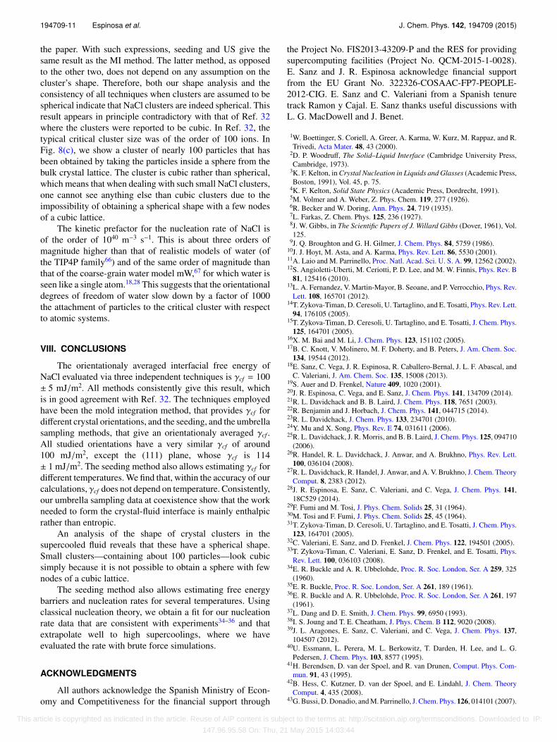
measuring the enthalpy of the system for each cluster sizeand subtracting the enthalpy of the liquid, we obtain theenthalpy of cluster formation as a function of the cluster sizeN. Then, we subtract N∆Hm to such enthalpy and divide by thecluster’s surface area (assuming a spherical shape) to obtainthe interfacial enthalpy Hcf . The interfacial entropy, Scf , isfinally obtained as S = (Hcf − γ)/T . In Fig. 14, we plot theinterfacial free energy and the two terms that add up to it (Hcf

and −T Scf ) as a function of the cluster size.As the cluster becomes larger, it is clear that γcf becomes

increasingly dominated by the enthalpic term. For the largestsimulated cluster (containing 210 particles) about 90% ofthe interfacial free energy is enthalpic. For such cluster size,the interfacial entropy is Scf = 0.01 mJ/m2 K, so small thatit would lead to a decrease of γ of only 3 mJ/m2 for asupercooling of 300 K. Such decrease is smaller than ourerror bar in the seeding method. From Fig. 14, it seems thatfor large clusters convergence will be reached for Hcf ≃ γ andScf ≃ 0. The fact that γcf for NaCl is mainly enthalpic cannotbe generalized to all systems. For instance, in water, the costto create the ice-fluid interface seems to be entropic ratherthan enthalpic.62 To conclude, the analysis performed from ourumbrella sampling simulations confirms the conclusion drawn

FIG. 14. Interfacial free energy (blue), interfacial enthalpy (red), and interfa-cial entropy multiplied by − T (green) as a function of the cluster size N.

from the seeding technique that γcf is either independent of Tor varies very smoothly with it.

VII. DISCUSSION

The orientationaly averaged γcf obtained through the threedifferent methodologies used in this work is about 100 mJ/m2.This value is consistent with that obtained in Ref. 32 assuminga spherical cluster shape. The value is also similar, althoughabout 10% higher, to that recently obtained by means of ananalysis of capillary wave fluctuations of the crystal-meltinterface.48 In order to get a good agreement between theγcf calculated for a planar interface (via MI or CapillaryFluctuations48) and that obtained from crystal clusters (seedingand US), we did not need to resort to corrections63 to thesimplest version of CNT. The value of 100 mN/m for γcf

clashes with the 36 mN/m obtained in Refs. 14 and 31.We suspect that the discrepancy may stem from finite sizeeffects such as the comparable weight of surface and linetensions, arising when calculating contact angles with smalldroplets.64 The good agreement between our results and thoseof Ref. 32 suggests that there are no irreducible size effects inthe calculation of γcf using small NaCl crystal clusters.33

The MI method gives γcf for different crystal orientations,whereas both seeding and US only provide an orientationalyaveraged γcf . Moreover, both seeding and US are subject to anassumption on the cluster shape and to an order parameter thatarbitrarily provides a value for the number of particles in thecrystal cluster. The MI method does not have these drawbacks,but in principle only allows to obtain a γcf at coexistence. Inorder to get the dependence of γcf with temperature, seedingis the best option. US is in principle also valid for thatpurpose, but it is computationally very expensive to computefree energy barriers at low supercoolings, where the criticalclusters contain thousands of particles. For NaCl, we find thatγcf does not depend on temperature (at constant pressure).This is not a general rule for all substances. For instance, recentstudies for water show that γcf decreases when the temperaturedecreases.18,28,62,65 Moreover, the seeding method permits theestimate of the nucleation rate as a function of temperaturethrough the calculation of the attachment rate of particlesto the critical cluster. The results are shown in Fig. 11(b)in purple squares and can be fitted using CNT (purple linein the same figure). The fit shows a good agreement withexperimental data.34–36 We have also used CNT to obtain anucleation rate curve for US and MI. Since γcf does not dependon temperature, one can take the average γcf calculated atcoexistence with these techniques and use CNT as we did tofit the seeding data to obtain the cyan curve shown in Fig. 11.Both US and MI give the same curve because they yield thesame average γcf . Of course, the curve is very close to thatobtained with seeding because all methods give very similarγcf (and γcf does not depend on T). Obtaining a nucleationcurve from MI or US at coexistence can only be attemptedif γcf does not depend on T (which, according to the seedingdata shown in Fig. 9, seems to be the case for NaCl).

In the seeding section of the paper, we show that theshape of crystal clusters is spherical. Consequently, we haveused the CNT expressions for a spherical cluster throughout

This article is copyrighted as indicated in the article. Reuse of AIP content is subject to the terms at: http://scitation.aip.org/termsconditions. Downloaded to IP:

147.96.95.58 On: Thu, 21 May 2015 14:03:44

194709-11 Espinosa et al. J. Chem. Phys. 142, 194709 (2015)

the paper. With such expressions, seeding and US give thesame result as the MI method. The latter method, as opposedto the other two, does not depend on any assumption on thecluster’s shape. Therefore, both our shape analysis and theconsistency of all techniques when clusters are assumed to bespherical indicate that NaCl clusters are indeed spherical. Thisresult appears in principle contradictory with that of Ref. 32where the clusters were reported to be cubic. In Ref. 32, thetypical critical cluster size was of the order of 100 ions. InFig. 8(c), we show a cluster of nearly 100 particles that hasbeen obtained by taking the particles inside a sphere from thebulk crystal lattice. The cluster is cubic rather than spherical,which means that when dealing with such small NaCl clusters,one cannot see anything else than cubic clusters due to theimpossibility of obtaining a spherical shape with a few nodesof a cubic lattice.

The kinetic prefactor for the nucleation rate of NaCl isof the order of 1040 m−3 s−1. This is about three orders ofmagnitude higher than that of realistic models of water (ofthe TIP4P family66) and of the same order of magnitude thanthat of the coarse-grain water model mW,67 for which water isseen like a single atom.18,28 This suggests that the orientationaldegrees of freedom of water slow down by a factor of 1000the attachment of particles to the critical cluster with respectto atomic systems.

VIII. CONCLUSIONS

The orientationaly averaged interfacial free energy ofNaCl evaluated via three independent techniques is γcf = 100± 5 mJ/m2. All methods consistently give this result, whichis in good agreement with Ref. 32. The techniques employedhave been the mold integration method, that provides γcf fordifferent crystal orientations, and the seeding, and the umbrellasampling methods, that give an orientationaly averaged γcf .All studied orientations have a very similar γcf of around100 mJ/m2, except the (111) plane, whose γcf is 114± 1 mJ/m2. The seeding method also allows estimating γcf fordifferent temperatures. We find that, within the accuracy of ourcalculations, γcf does not depend on temperature. Consistently,our umbrella sampling data at coexistence show that the workneeded to form the crystal-fluid interface is mainly enthalpicrather than entropic.

An analysis of the shape of crystal clusters in thesupercooled fluid reveals that these have a spherical shape.Small clusters—containing about 100 particles—look cubicsimply because it is not possible to obtain a sphere with fewnodes of a cubic lattice.

The seeding method also allows estimating free energybarriers and nucleation rates for several temperatures. Usingclassical nucleation theory, we obtain a fit for our nucleationrate data that are consistent with experiments34–36 and thatextrapolate well to high supercoolings, where we haveevaluated the rate with brute force simulations.

ACKNOWLEDGMENTS

All authors acknowledge the Spanish Ministry of Econ-omy and Competitiveness for the financial support through

the Project No. FIS2013-43209-P and the RES for providingsupercomputing facilities (Project No. QCM-2015-1-0028).E. Sanz and J. R. Espinosa acknowledge financial supportfrom the EU Grant No. 322326-COSAAC-FP7-PEOPLE-2012-CIG. E. Sanz and C. Valeriani from a Spanish tenuretrack Ramon y Cajal. E. Sanz thanks useful discussions withL. G. MacDowell and J. Benet.

1W. Boettinger, S. Coriell, A. Greer, A. Karma, W. Kurz, M. Rappaz, and R.Trivedi, Acta Mater. 48, 43 (2000).

2D. P. Woodruff, The Solid–Liquid Interface (Cambridge University Press,Cambridge, 1973).

3K. F. Kelton, in Crystal Nucleation in Liquids and Glasses (Academic Press,Boston, 1991), Vol. 45, p. 75.

4K. F. Kelton, Solid State Physics (Academic Press, Dordrecht, 1991).5M. Volmer and A. Weber, Z. Phys. Chem. 119, 277 (1926).6R. Becker and W. Doring, Ann. Phys. 24, 719 (1935).7L. Farkas, Z. Chem. Phys. 125, 236 (1927).8J. W. Gibbs, in The Scientific Papers of J. Willard Gibbs (Dover, 1961), Vol.125.

9J. Q. Broughton and G. H. Gilmer, J. Chem. Phys. 84, 5759 (1986).10J. J. Hoyt, M. Asta, and A. Karma, Phys. Rev. Lett. 86, 5530 (2001).11A. Laio and M. Parrinello, Proc. Natl. Acad. Sci. U. S. A. 99, 12562 (2002).12S. Angioletti-Uberti, M. Ceriotti, P. D. Lee, and M. W. Finnis, Phys. Rev. B

81, 125416 (2010).13L. A. Fernandez, V. Martin-Mayor, B. Seoane, and P. Verrocchio, Phys. Rev.

Lett. 108, 165701 (2012).14T. Zykova-Timan, D. Ceresoli, U. Tartaglino, and E. Tosatti, Phys. Rev. Lett.

94, 176105 (2005).15T. Zykova-Timan, D. Ceresoli, U. Tartaglino, and E. Tosatti, J. Chem. Phys.

125, 164701 (2005).16X. M. Bai and M. Li, J. Chem. Phys. 123, 151102 (2005).17B. C. Knott, V. Molinero, M. F. Doherty, and B. Peters, J. Am. Chem. Soc.

134, 19544 (2012).18E. Sanz, C. Vega, J. R. Espinosa, R. Caballero-Bernal, J. L. F. Abascal, and

C. Valeriani, J. Am. Chem. Soc. 135, 15008 (2013).19S. Auer and D. Frenkel, Nature 409, 1020 (2001).20J. R. Espinosa, C. Vega, and E. Sanz, J. Chem. Phys. 141, 134709 (2014).21R. L. Davidchack and B. B. Laird, J. Chem. Phys. 118, 7651 (2003).22R. Benjamin and J. Horbach, J. Chem. Phys. 141, 044715 (2014).23R. L. Davidchack, J. Chem. Phys. 133, 234701 (2010).24Y. Mu and X. Song, Phys. Rev. E 74, 031611 (2006).25R. L. Davidchack, J. R. Morris, and B. B. Laird, J. Chem. Phys. 125, 094710

(2006).26R. Handel, R. L. Davidchack, J. Anwar, and A. Brukhno, Phys. Rev. Lett.

100, 036104 (2008).27R. L. Davidchack, R. Handel, J. Anwar, and A. V. Brukhno, J. Chem. Theory

Comput. 8, 2383 (2012).28J. R. Espinosa, E. Sanz, C. Valeriani, and C. Vega, J. Chem. Phys. 141,

18C529 (2014).29F. Fumi and M. Tosi, J. Phys. Chem. Solids 25, 31 (1964).30M. Tosi and F. Fumi, J. Phys. Chem. Solids 25, 45 (1964).31T. Zykova-Timan, D. Ceresoli, U. Tartaglino, and E. Tosatti, J. Chem. Phys.

123, 164701 (2005).32C. Valeriani, E. Sanz, and D. Frenkel, J. Chem. Phys. 122, 194501 (2005).33T. Zykova-Timan, C. Valeriani, E. Sanz, D. Frenkel, and E. Tosatti, Phys.

Rev. Lett. 100, 036103 (2008).34E. R. Buckle and A. R. Ubbelohde, Proc. R. Soc. London, Ser. A 259, 325

(1960).35E. R. Buckle, Proc. R. Soc. London, Ser. A 261, 189 (1961).36E. R. Buckle and A. R. Ubbelohde, Proc. R. Soc. London, Ser. A 261, 197

(1961).37L. Dang and D. E. Smith, J. Chem. Phys. 99, 6950 (1993).38I. S. Joung and T. E. Cheatham, J. Phys. Chem. B 112, 9020 (2008).39J. L. Aragones, E. Sanz, C. Valeriani, and C. Vega, J. Chem. Phys. 137,

104507 (2012).40U. Essmann, L. Perera, M. L. Berkowitz, T. Darden, H. Lee, and L. G.

Pedersen, J. Chem. Phys. 103, 8577 (1995).41H. Berendsen, D. van der Spoel, and R. van Drunen, Comput. Phys. Com-

mun. 91, 43 (1995).42B. Hess, C. Kutzner, D. van der Spoel, and E. Lindahl, J. Chem. Theory

Comput. 4, 435 (2008).43G. Bussi, D. Donadio, and M. Parrinello, J. Chem. Phys. 126, 014101 (2007).

This article is copyrighted as indicated in the article. Reuse of AIP content is subject to the terms at: http://scitation.aip.org/termsconditions. Downloaded to IP:

147.96.95.58 On: Thu, 21 May 2015 14:03:44

194709-12 Espinosa et al. J. Chem. Phys. 142, 194709 (2015)

44M. Parrinello and A. Rahman, J. Appl. Phys. 52, 7182 (1981).45T. Schilling and F. Schmid, J. Chem. Phys. 131, 231102 (2009).46J. R. Espinosa, E. Sanz, C. Valeriani, and C. Vega, J. Chem. Phys. 139,

144502 (2013).47P. W. Tasker, J. Phys. C: Solid State Phys. 12, 4977 (1979).48J. Benet, L. G. MacDowell, and E. Sanz, J. Chem. Phys. 142, 134706 (2015).49X. M. Bai and M. Li, J. Chem. Phys. 124, 124707 (2006).50R. G. Pereyra, I. Szleifer, and M. A. Carignano, J. Chem. Phys. 135, 034508

(2011).51S. Auer and D. Frenkel, J. Chem. Phys. 120, 3015 (2004).52P. R. ten Wolde, M. J. Ruiz-Montero, and D. Frenkel, J. Chem. Phys. 104,

9932 (1996).53P. R. ten Wolde, M. J. Ruiz-Montero, and D. Frenkel, Phys. Rev. Lett. 75,

2714 (1995).54D. Turnbull, J. Appl. Phys. 21, 1022 (1950).55R. S. Aga, J. R. Morris, J. J. Hoyt, and M. Mendelev, Phys. Rev. Lett. 96,

245701 (2006).

56L. J. Peng, J. R. Morris, and R. S. Aga, J. Chem. Phys. 133, 084505(2010).

57G. M. Torrie and J. P. Valleau, J. Comput. Phys. 23, 187 (1977).58P. R. ten Wolde and D. Frenkel, J. Chem. Phys. 109, 9901 (1998).59A. Cacciuto, S. Auer, and D. Frenkel, J. Chem. Phys. 119, 7467 (2003).60J. Rowlinson and B. Widom, Molecular Theory of Capillarity, Dover Books

on Chemistry (Dover Publications, 2002).61J. Anwar, D. Frenkel, and M. G. Noro, J. Chem. Phys. 118, 728 (2003).62A. Reinhardt and J. P. K. Doye, J. Chem. Phys. 139, 096102 (2013).63S. Prestipino, A. Laio, and E. Tosatti, Phys. Rev. Lett. 108, 225701 (2012).64L. G. MacDowell, M. Müller, and K. Binder, Colloids Surf., A 206, 277

(2002).65L. Ickes, A. Welti, C. Hoose, and U. Lohmann, Phys. Chem. Chem. Phys.

17, 5514 (2015).66W. L. Jorgensen, J. Chandrasekhar, J. D. Madura, R. W. Impey, and M. L.

Klein, J. Chem. Phys. 79, 926 (1983).67V. Molinero and E. B. Moore, J. Phys. Chem. B 113, 4008 (2009).

This article is copyrighted as indicated in the article. Reuse of AIP content is subject to the terms at: http://scitation.aip.org/termsconditions. Downloaded to IP:

147.96.95.58 On: Thu, 21 May 2015 14:03:44