The Cross-Section of Volatility and Expected Returns∗

Andrew Ang†

Columbia University, USC and NBER

Robert J. Hodrick‡

Columbia University and NBER

Yuhang Xing§

Rice University

Xiaoyan Zhang¶

Cornell University

This Version: 1 October, 2004

∗We thank Joe Chen, Mike Chernov, Miguel Ferreira, Jeff Fleming, Chris Lamoureux, Jun Liu, Lau-rie Hodrick, Paul Hribar, Jun Pan, Matt Rhodes-Kropf, Steve Ross, David Weinbaum, and Lu Zhangfor helpful discussions. We also received valuable comments from seminar participants at an NBERAsset Pricing meeting, Campbell and Company, Columbia University, Cornell University, Hong KongUniversity, Rice University, UCLA, and the University of Rochester. We thank Tim Bollerslev, JoeChen, Miguel Ferreira, Kenneth French, Anna Scherbina, and Tyler Shumway for kindly providing data.We especially thank an anonymous referee and Rob Stambaugh, the editor, for helpful suggestions thatgreatly improved the article. Andrew Ang and Bob Hodrick both acknowledge support from the NSF.

†Marshall School of Business, USC, 701 Exposition Blvd, Room 701, Los Angeles, CA 90089. Ph:213 740 5615, Email: aa610@columbia.edu, WWW: http://www.columbia.edu/∼aa610.

‡Columbia Business School, 3022 Broadway Uris Hall, New York, NY 10027. Ph: (212) 854-0406,Email: rh169@columbia.edu, WWW: http://www.columbia.edu/∼rh169.

§Jones School of Management, Rice University, Rm 230, MS 531, 6100 Main Street, Houston TX77004. Ph: (713) 348-4167, Email: yxing@rice.edu; WWW: http://www.ruf.rice.edu/ yxing

¶336 Sage Hall, Johnson Graduate School of Management, Cornell University, Ithaca NY 14850.Ph: (607) 255-8729 Email: xz69@cornell.edu, WWW: http://www.johnson.cornell.edu/faculty/pro-files/xZhang/

Abstract

We examine the pricing of aggregate volatility risk in the cross-section of stock returns.

Consistent with theory, we find that stocks with high sensitivities to innovations in aggregate

volatility have low average returns. In addition, we find that stocks with high idiosyncratic

volatility relative to the Fama and French (1993) model have abysmally low average returns.

This phenomenon cannot be explained by exposure to aggregate volatility risk. Size, book-

to-market, momentum, and liquidity effects cannot account for either the low average returns

earned by stocks with high exposure to systematic volatility risk or for the low average returns

of stocks with high idiosyncratic volatility.

It is well known that the volatility of stock returns varies over time. While considerable

research has examined the time-series relation between the volatility of the market and the ex-

pected return on the market (see, among others, Campbell and Hentschel (1992), and Glosten,

Jagannathan and Runkle (1993)), the question of how aggregate volatility affects the cross-

section of expected stock returns has received less attention. Time-varying market volatility

induces changes in the investment opportunity set by changing the expectation of future mar-

ket returns, or by changing the risk-return trade-off. If the volatility of the market return is a

systematic risk factor, an APT or factor model predicts that aggregate volatility should also be

priced in the cross-section of stocks. Hence, stocks with different sensitivities to innovations in

aggregate volatility should have different expected returns.

The first goal of this paper is to provide a systematic investigation of how the stochastic

volatility of the market is priced in the cross-section of expected stock returns. We want to de-

termine if the volatility of the market is a priced risk factor and estimate the price of aggregate

volatility risk. Many option studies have estimated a negative price of risk for market volatility

using options on an aggregate market index or options on individual stocks.1 Using the cross-

section of stock returns, rather than options on the market, allows us to create portfolios of

stocks that have different sensitivities to innovations in market volatility. If the price of aggre-

gate volatility risk is negative, stocks with large, positive sensitivities to volatility risk should

have low average returns. Using the cross-section of stock returns also allows us to easily con-

trol for a battery of cross-sectional effects, like the size and value factors of Fama and French

(1993), the momentum effect of Jegadeesh and Titman (1993), and the effect of liquidity risk

documented by Pastor and Stambaugh (2003). Option pricing studies do not control for these

cross-sectional risk factors.

We find that innovations in aggregate volatility carry a statistically significant negative price

of risk of approximately -1% per annum. Economic theory provides several reasons why the

price of risk of innovations in market volatility should be negative. For example, Campbell

(1993 and 1996) and Chen (2002) show that investors want to hedge against changes in mar-

ket volatility, because increasing volatility represents a deterioration in investment opportuni-

ties. Risk averse agents demand stocks that hedge against this risk. Periods of high volatility

also tend to coincide with downward market movements (see French, Schwert and Stambaugh

(1987), and Campbell and Hentschel (1992)). As Bakshi and Kapadia (2003) comment, assets

with high sensitivities to market volatility risk provide hedges against market downside risk.

The higher demand for assets with high systematic volatility loadings increases their price and

1

lowers their average return. Finally, stocks that do badly when volatility increases tend to have

negatively skewed returns over intermediate horizons, while stocks that do well when volatil-

ity rises tend to have positively skewed returns. If investors have preferences over coskewness

(see Harvey and Siddique (2000)), stocks that have high sensitivities to innovations in market

volatility are attractive and have low returns.2

The second goal of the paper is to examine the cross-sectional relationship between id-

iosyncratic volatility and expected returns, where idiosyncratic volatility is defined relative to

the standard Fama and French (1993) model.3 If the Fama-French model is correct, forming

portfolios by sorting on idiosyncratic volatility will obviously provide no difference in average

returns. Nevertheless, if the Fama-French model is false, sorting in this way potentially provides

a set of assets that may have different exposures to aggregate volatility and hence different aver-

age returns. Our logic is the following. If aggregate volatility is a risk factor that is orthogonal

to existing risk factors, the sensitivity of stocks to aggregate volatility times the movement in

aggregate volatility will show up in the residuals of the Fama-French model. Firms with greater

sensitivities to aggregate volatility should therefore have larger idiosyncratic volatilities relative

to the Fama-French model, everything else being equal. Differences in the volatilities of firms’

true idiosyncratic errors, which are not priced, will make this relation noisy. We should be able

to average out this noise by constructing portfolios of stocks to reveal that larger idiosyncratic

volatilities relative to the Fama-French model correspond to greater sensitivities to movements

in aggregate volatility and thus different average returns, if aggregate volatility risk is priced.

While high exposure to aggregate volatility risk tends to produce low expected returns, some

economic theories suggest that idiosyncratic volatility should be positively related to expected

returns. If investors demand compensation for not being able to diversify risk (see Malkiel

and Xu (2002), and Jones and Rhodes-Kropf (2003)), then agents will demand a premium for

holding stocks with high idiosyncratic volatility. Merton (1987) suggests that in an information-

segmented market, firms with larger firm-specific variances require higher average returns to

compensate investors for holding imperfectly diversified portfolios. Some behavioral models,

like Barberis and Huang (2001), also predict that higher idiosyncratic volatility stocks should

earn higher expected returns. Our results are directly opposite to these theories. We find that

stocks with high idiosyncratic volatility have low average returns. There is a strongly significant

difference of -1.06% per month between the average returns of the quintile portfolio with the

highest idiosyncratic volatility stocks and the quintile portfolio with the lowest idiosyncratic

volatility stocks.

2

In contrast to our results, earlier researchers either found a significantly positive relation

between idiosyncratic volatility and average returns, or they failed to find any statistically sig-

nificant relation between idiosyncratic volatility and average returns. For example, Lintner

(1965) shows that idiosyncratic volatility carries a positive coefficient in cross-sectional regres-

sions. Lehmann (1990) also finds a statistically significant, positive coefficient on idiosyncratic

volatility over his full sample period. Similarly, Tinic and West (1986) and Malkiel and Xu

(2002) unambiguously find that portfolios with higher idiosyncratic volatility have higher av-

erage returns, but they do not report any significance levels for their idiosyncratic volatility

premiums. On the other hand, Longstaff (1989) finds that a cross-sectional regression coeffi-

cient on total variance for size-sorted portfolios carries an insignificant negative sign.

The difference between our results and the results of past studies is that the past literature

either does not examine idiosyncratic volatility at the firm level or does not directly sort stocks

into portfolios ranked on this measure of interest. For example, Tinic and West (1986) work

only with 20 portfolios sorted on market beta, while Malkiel and Xu (2002) work only with

100 portfolios sorted on market beta and size. Malkiel and Xu (2002) only use the idiosyncratic

volatility of one of the 100 beta/size portfolios to which a stock belongs to proxy for that stock’s

idiosyncratic risk and, thus, do not examine firm-level idiosyncratic volatility. Hence, by not di-

rectly computing differences in average returns between stocks with low and high idiosyncratic

volatilities, previous studies miss the strong negative relation between idiosyncratic volatility

and average returns that we find.

The low average returns to stocks with high idiosyncratic volatilities could arise because

stocks with high idiosyncratic volatilities may have high exposure to aggregate volatility risk,

which lowers their average returns. We investigate this issue and find that this is not a complete

explanation. Our idiosyncratic volatility results are also robust to controlling for value, size,

liquidity, volume, dispersion of analysts’ forecasts, and momentum effects. We find the effect

robust to different formation periods for computing idiosyncratic volatility and for different

holding periods. The effect also persists in both bull and bear markets, recessions and expan-

sions, and volatile and stable periods. Hence, our results on idiosyncratic volatility represent a

substantive puzzle.

The rest of this paper is organized as follows. In Section I, we examine how aggregate

volatility is priced in the cross-section of stock returns. Section II documents that firms with

high idiosyncratic volatility have very low average returns. Finally, Section III concludes.

3

I. Pricing Systematic Volatility in the Cross-Section

A. Theoretical Motivation

When investment opportunities vary over time, the multi-factor models of Merton (1973) and

Ross (1976) show that risk premia are associated with the conditional covariances between as-

set returns and innovations in state variables that describe the time-variation of the investment

opportunities. Campbell’s (1993 and 1996) version of the Intertemporal CAPM (I-CAPM)

shows that investors care about risks from the market return and from changes in forecasts of

future market returns. When the representative agent is more risk averse than log utility, assets

that covary positively with good news about future expected returns on the market have higher

average returns. These assets command a risk premium because they reduce a consumer’s abil-

ity to hedge against a deterioration in investment opportunities. The intuition from Campbell’s

model is that risk-averse investors want to hedge against changes in aggregate volatility because

volatility positively affects future expected market returns, as in Merton (1973).

However, in Campbell’s set-up, there is no direct role for fluctuations in market volatility to

affect the expected returns of assets because Campbell’s model is premised on homoskedastic-

ity. Chen (2002) extends Campbell’s model to a heteroskedastic environment which allows for

both time-varying covariances and stochastic market volatility. Chen shows that risk-averse in-

vestors also want to directly hedge against changes in future market volatility. In Chen’s model,

an asset’s expected return depends on risk from the market return, changes in forecasts of future

market returns, and changes in forecasts of future market volatilities. For an investor more risk

averse than log utility, Chen shows that an asset that has a positive covariance between its return

and a variable that positively forecasts future market volatilities causes that asset to have a lower

expected return. This effect arises because risk-averse investors reduce current consumption to

increase precautionary savings in the presence of increased uncertainty about market returns.

Motivated by these multi-factor models, we study how exposure to market volatility risk is

priced in the cross-section of stock returns. A true conditional multi-factor representation of

expected returns in the cross-section would take the following form:

rit+1 = ai

t + βim,t(r

mt+1 − γm,t) + βi

v,t(vt+1 − γv,t) +K∑

k=1

βik,t(fk,t+1 − γk,t), (1)

whererit+1 is the excess return on stocki, βi

m,t is the loading on the excess market return,βiv,t

is the asset’s sensitivity to volatility risk, and theβik,t coefficients fork = 1 . . . K represent

4

loadings on other risk factors. In the full conditional setting in equation (1), factor loadings,

conditional means of factors, and factor premiums potentially vary over time. The model in

equation (1) is written in terms of factor innovations, sormt+1− γm,t represents the innovation in

the market return,vt+1−γv,t represents the innovation in the factor reflecting aggregate volatility

risk, and innovations to the other factors are represented byfk,t+1 − γk,t. The conditional

mean of the market and aggregate volatility are denoted byγm,t andγv,t, respectively, while the

conditional mean of the other factors are denoted byγk,t. In equilibrium, the conditional mean

of stocki is given by:

ait = Et(r

it+1) = βi

m,tλm,t + βiv,tλv,t +

K∑

k=1

βik,tλk,t, (2)

whereλm,t is the price of risk of the market factor,λv,t is the price of aggregate volatility risk,

and theλk,t are prices of risk of the other factors. Note that only if a factor is traded is the

conditional mean of a factor equal to its conditional price of risk.

The main prediction from the factor model setting of equation (1) that we examine is that

stocks with different loadings on aggregate volatility risk have different average returns.4 How-

ever, the true model in equation (1) is infeasible to examine because the true set of factors is

unknown and the true conditional factor loadings are unobservable. Hence, we do not attempt to

directly use equation (1) in our empirical work. Instead, we simplify the full model in equation

(1), which we now detail.

B. The Empirical Framework

To investigate how aggregate volatility risk is priced in the cross-section of equity returns we

make the following simplifying assumptions to the full specification in equation (1). First, we

use observable proxies for the market factor and the factor representing aggregate volatility risk.

We use the CRSP value-weighted market index to proxy for the market factor. To proxy innova-

tions in aggregate volatility,(vt+1 − γv,t), we use changes in theV IX index from the Chicago

Board Options Exchange (CBOE).5 Second, we reduce the number of factors in equation (1)

to just the market factor and the proxy for aggregate volatility risk. Finally, to capture the con-

ditional nature of the true model, we use short intervals, one month of daily data, to take into

account possible time-variation of the factor loadings. We discuss each of these simplifications

in turn.

5

B.1. Innovations in theV IX Index

TheV IX index is constructed so that it represents the implied volatility of a synthetic at-the-

money option contract on the S&P100 index that has a maturity of one month. It is constructed

from eight S&P100 index puts and calls and takes into account the American features of the

option contracts, discrete cash dividends and microstructure frictions such as bid-ask spreads

(see Whaley (2000) for further details).6 Figure 1 plots theV IX index from January 1986 to

December 2000. The mean level of the dailyV IX series is 20.5%, and its standard deviation

is 7.85%.

[FIGURE 1 ABOUT HERE]

Because theV IX index is highly serially correlated with a first-order autocorrelation of

0.94, we measure daily innovations in aggregate volatility by using daily changes inV IX,

which we denote as∆V IX. Daily first differences inV IX have an effective mean of zero (less

than 0.0001), a standard deviation of 2.65%, and also have negligible serial correlation (the

first-order autocorrelation of∆V IX is -0.0001). As part of our robustness checks in Section

C, we also measure innovations inV IX by specifying a stationary time-series model for the

conditional mean ofV IX and find our results to be similar to using simple first differences.

While ∆V IX seems an ideal proxy for innovations in volatility risk because theV IX index is

representative of traded option securities whose prices directly reflect volatility risk, there are

two main caveats with usingV IX to represent observable market volatility.

The first concern is that theV IX index is the implied volatility from the Black-Scholes

(1973) model, and we know that the Black-Scholes model is an approximation. If the true

stochastic environment is characterized by stochastic volatility and jumps,∆V IX will reflect

total quadratic variation in both diffusion and jump components (see, for example, Pan (2002)).

Although Bates (2000) argues that implied volatilities computed taking into account jump risk

are very close to original Black-Scholes implied volatilities, jump risk may be priced differ-

ently from volatility risk. Our analysis does not separate jump risk from diffusion risk, so our

aggregate volatility risk may include jump risk components.

A more serious reservation about theV IX index is thatV IX combines both stochastic

volatility and the stochastic volatility risk premium. Only if the risk premium is zero or constant

would∆V IX be a pure proxy for the innovation in aggregate volatility. Decomposing∆V IX

into the true innovation in volatility and the volatility risk premium can only be done by writing

6

down a formal model. The form of the risk premium depends on the parameterization of the

price of volatility risk, the number of factors and the evolution of those factors. Each different

model specification implies a different risk premium. For example, many stochastic volatility

option pricing models assume that the volatility risk premium can be parameterized as a linear

function of volatility (see, for example, Chernov and Ghysels (2000), Benzoni (2002), and

Jones (2003)). This may or may not be a good approximation to the true price of risk. Rather

than imposing a structural form, we use an unadulterated∆V IX series. An advantage of this

approach is that our analysis is simple to replicate.

B.2. The Pre-Formation Regression

Our goal is to test if stocks with different sensitivities to aggregate volatility innovations (prox-

ied by∆V IX) have different average returns. To measure the sensitivity to aggregate volatility

innovations, we reduce the number of factors in the full specification in equation (1) to two, the

market factor and∆V IX. A two-factor pricing kernel with the market return and stochastic

volatility as factors is also the standard set-up commonly assumed by many stochastic option

pricing studies (see, for example, Heston, 1993). Hence, the empirical model that we examine

is:

rit = β0 + βi

MKT ·MKTt + βi∆V IX ·∆V IXt + εi

t, (3)

whereMKT is the market excess return,∆V IX is the instrument we use for innovations in

the aggregate volatility factor, andβiMKT andβi

∆V IX are loadings on market risk and aggregate

volatility risk, respectively.

Previous empirical studies suggest that there are other cross-sectional factors that have ex-

planatory power for the cross-section of returns, such as the size and value factors of the Fama

and French (1993) three-factor model (hereafter FF-3). We do not directly model these effects

in equation (3), because controlling for other factors in constructing portfolios based on equa-

tion (3) may add a lot of noise. Although we keep the number of regressors in our pre-formation

portfolio regressions to a minimum, we are careful to ensure that we control for the FF-3 factors

and other cross-sectional factors in assessing how volatility risk is priced using post-formation

regression tests.

We construct a set of assets that are sufficiently disperse in exposure to aggregate volatility

innovations by sorting firms on∆V IX loadings over the past month using the regression (3)

with daily data. We run the regression for all stocks on AMEX, NASDAQ and the NYSE, with

more than 17 daily observations. In a setting where coefficients potentially vary over time, a

7

1-month window with daily data is a natural compromise between estimating coefficients with

a reasonable degree of precision and pinning down conditional coefficients in an environment

with time-varying factor loadings. Pastor and Stambaugh (2003), among others, also use daily

data with a 1-month window in similar settings. At the end of each month, we sort stocks into

quintiles, based on the value of the realizedβ∆V IX coefficients over the past month. Firms in

quintile 1 have the lowest coefficients, while firms in quintile 5 have the highestβ∆V IX loadings.

Within each quintile portfolio, we value-weight the stocks. We link the returns across time to

form one series of post-ranking returns for each quintile portfolio.

Table I reports various summary statistics for quintile portfolios sorted by pastβ∆V IX over

the previous month using equation (3). The first two columns report the mean and standard

deviation of monthly total, not excess, simple returns. In the first column under the heading

‘Factor Loadings,’ we report the pre-formationβ∆V IX coefficients, which are computed at the

beginning of each month for each portfolio and are value-weighted. The column reports the

time-series average of the pre-formationβ∆V IX loadings across the whole sample. By con-

struction, since the portfolios are formed by ranking on pastβ∆V IX , the pre-formationβ∆V IX

loadings monotonically increase from -2.09 for portfolio 1 to 2.18 for portfolio 5.

[TABLE I ABOUT HERE]

The columns labelled ‘CAPM Alpha’ and ‘FF-3 Alpha’ report the time-series alphas of

these portfolios relative to the CAPM and to the FF-3 model, respectfully. Consistent with the

negative price of systematic volatility risk found by the option pricing studies, we see lower

average raw returns, CAPM alphas, and FF-3 alphas with higher past loadings ofβ∆V IX . All

the differences between quintile portfolios 5 and 1 are significant at the 1% level, and a joint test

for the alphas equal to zero rejects at the 5% level for both the CAPM and the FF-3 model. In

particular, the 5-1 spread in average returns between the quintile portfolios with the highest and

lowestβ∆V IX coefficients is -1.04% per month. Controlling for theMKT factor exacerbates

the 5-1 spread to -1.15% per month, while controlling for the FF-3 model decreases the 5-1

spread to -0.83% per month.

B.3. Requirements for a Factor Risk Explanation

While the differences in average returns and alphas corresponding to differentβ∆V IX loadings

are very impressive, we cannot yet claim that these differences are due to systematic volatility

8

risk. We will examine the premium for aggregate volatility within the framework of an uncon-

ditional factor model. There are two requirements that must hold in order to make a case for a

factor risk-based explanation. First, a factor model implies that there should be contemporane-

ous patterns between factor loadings and average returns. For example, in a standard CAPM,

stocks that covary strongly with the market factor should, on average, earn high returns over the

same period. To test a factor model, Black, Jensen and Scholes (1972), Fama and French (1992

and 1993), Jagannathan and Wang (1996), and Pastor and Stambaugh (2003), among others, all

form portfolios using various pre-formation criteria, but examine post-ranking factor loadings

that are computed over the full sample period. While theβ∆V IX loadings show very strong

patterns of future returns, they represent past covariation with innovations in market volatility.

We must show that the portfolios in Table I also exhibit high loadings with volatility risk over

the same period used to compute the alphas.

To construct our portfolios, we took∆V IX to proxy for the innovation in aggregate volatil-

ity at a daily frequency. However, at the standard monthly frequency, which is the frequency

of the ex-post returns for the alphas reported in Table I, using the change inV IX is a poor

approximation for innovations in aggregate volatility. This is because at lower frequencies, the

effect of the conditional mean ofV IX plays an important role in determining the unanticipated

change inV IX. In contrast, the high persistence of theV IX series at a daily frequency means

that the first difference ofV IX is a suitable proxy for the innovation in aggregate volatility.

Hence, we should not measure ex-post exposure to aggregate volatility risk by looking at how

the portfolios in Table I correlate ex-post with monthly changes inV IX.

To measure ex-post exposure to aggregate volatility risk at a monthly frequency, we follow

Breeden, Gibbons and Litzenberger (1989) and construct an ex-post factor that mimics aggre-

gate volatility risk. We term this mimicking factorFV IX. We construct the tracking portfolio

so that it is the portfolio of asset returns maximally correlated with realized innovations in

volatility using a set of basis assets. This allows us to examine the contemporaneous relation-

ship between factor loadings and average returns. The major advantage of usingFV IX to

measure aggregate volatility risk is that we can construct a good approximation for innovations

in market volatility at any frequency. In particular, the factor mimicking aggregate volatility

innovations allows us to proxy aggregate volatility risk at the monthly frequency by simply

cumulating daily returns over the month on the underlying base assets used to construct the

mimicking factor. This is a much simpler method for measuring aggregate volatility innova-

tions at different frequencies, rather than specifying different, and unknown, conditional means

9

for V IX that depend on different sampling frequencies. After constructing the mimicking ag-

gregate volatility factor, we will confirm that it is high exposure to aggregate volatility risk that

is behind the low average returns to pastβ∆V IX loadings.

However, just showing that there is a relation between ex-post aggregate volatility risk expo-

sure and average returns does not rule out the explanation that the volatility risk exposure is due

to known determinants of expected returns in the cross-section. Hence, our second condition for

a risk-based explanation is that the aggregate volatility risk exposure is robust to controlling for

various stock characteristics and other factor loadings. Several of these cross-sectional effects

may be at play in the results of Table I. For example, quintile portfolios 1 and 5 have smaller

stocks, and stocks with higher book-to-market ratios, and these are the portfolios with the most

extreme returns. Periods of very high volatility also tend to coincide with periods of market

illiquidity (see, among others, Jones (2003) and Pastor and Stambaugh (2003)). In Section C,

we control for size, book-to-market, and momentum effects, and also specifically disentangle

the exposure to liquidity risk from the exposure to systematic volatility risk.

B.4. A Factor Mimicking Aggregate Volatility Risk

Following Breeden, Gibbons and Litzenberger (1989) and Lamont (2001), we create the mim-

icking factorFV IX to track innovations inV IX by estimating the coefficientb in the following

regression:

∆V IXt = c + b′Xt + ut, (4)

whereXt represents the returns on the base assets. Since the base assets are excess returns,

the coefficientb has the interpretation of weights in a zero-cost portfolio. The return on the

portfolio, b′Xt, is the factorFV IX that mimics innovations in market volatility. We use the

quintile portfolios sorted on pastβ∆V IX in Table I as the base assetsXt. These base assets are,

by construction, a set of assets that have different sensitivities to past daily innovations inV IX.7

We run the regression in equation (4) at a daily frequency every month and use the estimates of

b to construct the mimicking factor for aggregate volatility risk over the same month.

An alternative way to construct a factor that mimics volatility risk is to directly construct a

traded asset that reflects only volatility risk. One way to do this is to consider option returns.

Coval and Shumway (2001) construct market-neutral straddle positions using options on the

aggregate market (S&P 100 options). This strategy provides exposure to aggregate volatility

risk. Coval and Shumway approximate daily at-the-money straddle returns by taking a weighted

average of zero-beta straddle positions, with strikes immediately above and below each day’s

10

opening level of the S&P 100. They cumulate these daily returns each month to form a monthly

return, which we denote asSTR.8 In Section D, we investigate the robustness of our results to

usingSTR in place ofFV IX when we estimate the cross-sectional aggregate volatility price

of risk.

Once we constructFV IX, then the multi-factor model (3) holds, except we can substitute

the (unobserved) innovation in volatility with the tracking portfolio that proxies for market

volatility risk (see Breeden (1979)). Hence, we can write the model in equation (3) as the

following cross-sectional regression:

rit = αi + βi

MKT ·MKTt + βiFV IX · FV IXt + εi

t (5)

whereMKT is the market excess return,FV IX is the mimicking aggregate volatility factor,

andβiMKT andβi

FV IX are factor loadings on market risk and aggregate volatility risk, respec-

tively.

To test a factor risk model like equation (5), we must show contemporaneous patterns be-

tween factor loadings and average returns. That is, if the price of risk of aggregate volatility is

negative, then stocks with high covariation withFV IX should have low returns, on average,

over the same period used to compute theβFV IX factor loadings and the average returns. By

construction,FV IX allows us to examine the contemporaneous relationship between factor

loadings and average returns and it is the factor that is ex-post most highly correlated with in-

novations in aggregate volatility. However, whileFV IX is the right factor to test a risk story,

FV IX itself is not an investable portfolio because it is formed with future information. Nev-

ertheless,FV IX can be used as guidance for tradeable strategies that would hedge market

volatility risk using the cross-section of stocks.

In the second column under the heading ‘Factor Loadings’ of Table I, we report the pre-

formationβFV IX loadings that correspond to each of the portfolios sorted on pastβ∆V IX load-

ings. The pre-formationβFV IX loadings are computed by running the regression (5) over daily

returns over the past month. The pre-formationFV IX loadings are very similar to the pre-

formation∆V IX loadings for the portfolios sorted on pastβ∆V IX loadings. For example, the

pre-formationβFV IX (β∆V IX) loading for quintile 1 is -2.00 (-2.09), while the pre-formation

βFV IX (β∆V IX) loading for quintile 5 is 2.31 (2.18).

11

B.5. Post-Formation Factor Loadings

In the next to last column of Table I, we report post-formationβ∆V IX loadings over the next

month, which we compute as follows. After the quintile portfolios are formed at timet, we

calculate daily returns of each of the quintile portfolios over the next month, fromt to t+1. For

each portfolio, we compute the ex-postβ∆V IX loadings by running the same regression (3) that

is used to form the portfolios using daily data over the next month (t to t+1). We report the next

monthβ∆V IX loadings averaged across time. The next month post-formationβ∆V IX loadings

range from -0.033 for portfolio 1 to 0.018 for portfolio 5. Hence, although the ex-postβ∆V IX

loadings over the next month are monotonically increasing, the spread is disappointingly very

small.

Finding large spreads in the next month post-formationβ∆V IX loadings is a very stringent

requirement and one that would be done in direct tests of a conditional factor model like equa-

tion (1). Our goal is more modest. We examine the premium for aggregate volatility using

an unconditional factor model approach, which requires that average returns are related to the

unconditional covariation between returns and aggregate volatility risk. As Hansen and Richard

(1987) note, an unconditional factor model implies the existence of a conditional factor model.

However, to form precise estimates of the conditional factor loadings in a full conditional set-

ting like equation (1) requires knowledge of the instruments driving the time-variation in the

betas, as well as specifying the complete set of factors.

The ex-postβ∆V IX loadings over the next month are computed using, on average, only 22

daily observations each month. In contrast, the CAPM and FF-3 alphas are computed using

regressions measuring unconditional factor exposure over the full sample (180 monthly obser-

vations) of post-ranking returns. To demonstrate that exposure to volatility innovations may

explain some of the large CAPM and FF-3 alphas, we must show that the quintile portfolios

exhibit different post-ranking spreads in aggregate volatility risk sensitivities over the entire

sample at the same monthly frequency for which the post-ranking returns are constructed. Av-

eraging a series of ex-post conditional one month covariances does not provide an estimate of

the unconditional covariation between the portfolio returns and aggregate volatility risk.

To examine ex-post factor exposure to aggregate volatility risk consistent with a factor

model approach, we compute post-rankingFV IX betas over the full sample.9 In particular,

since the FF-3 alpha controls for market, size, and value factors, we compute ex-postFV IX

12

factor loadings also controlling for these factors in a 4-factor post-formation regression:

rit = αi + βi

MKT ·MKTt + +βiSMB · SMBt + βi

HML ·HMLt + βiFV IX · FV IXt + εi

t, (6)

where the first three factorsMKT , SMB andHML constitute the FF-3 model’s market, size

and value factors. To compute the ex-postβFV IX loadings, we run equation (6) using monthly

frequency data over the whole sample, where the portfolios on the LHS of equation (6) are the

quintile portfolios in Table I that are sorted on past loadings ofβ∆V IX using equation (3).

The last column of Table I shows that the portfolios sorted on pastβ∆V IX exhibit strong

patterns of post-formation factor loadings on the volatility risk factorFV IX. The ex-post

βFV IX factor loadings monotonically increase from -5.06 for portfolio 1 to 8.07 for portfolio

5. We strongly reject the hypothesis that the ex-postβFV IX loadings are equal to zero, with a

p-value less than 0.001. Thus, sorting stocks on pastβ∆V IX provides strong, significant spreads

in ex-post aggregate volatility risk sensitivities.10

B.6. Characterizing the Behavior ofFV IX

Table II reports correlations between theFV IX factor,∆V IX, andSTR, as well as correla-

tions of these variables with other cross-sectional factors. We denote the daily first difference

in V IX as∆V IX, and use∆mV IX to represent the monthly first difference in theV IX in-

dex. The mimicking volatility factor is highly contemporaneously correlated with changes in

volatility at a daily frequency, with a correlation of 0.91. At the monthly frequency, the cor-

relation betweenFV IX and∆mV IX is lower, at 0.70. The factorsFV IX andSTR have a

high correlation of 0.83, which indicates thatFV IX, formed from stock returns, behaves like

theSTR factor constructed from option returns. Hence,FV IX captures option-like behavior

in the cross-section of stocks. The factorFV IX is negatively contemporaneously correlated

with the market return (-0.66), reflecting the fact that when volatility increases, market returns

are low. The correlations ofFV IX with SMB andHML are -0.14 and 0.26, respectively.

The correlation betweenFV IX andUMD, a factor capturing momentum returns, is also low

at -0.25.

[TABLE II ABOUT HERE]

In contrast, there is a strong negative correlation betweenFV IX and the Pastor and Stam-

baugh (2003) liquidity factor,LIQ, at -0.40. TheLIQ factor decreases in times of low liquidity,

13

which tend to also be periods of high volatility. One example of a period of low liquidity with

high volatility is the 1987 crash (see, among others, Jones (2003) and Pastor and Stambaugh

(2003)). However, the correlation betweenFV IX and LIQ is far from -1, indicating that

volatility risk and liquidity risk may be separate effects, and may be separately priced. In the

next section, we conduct a series of robustness checks designed to disentangle the effects of

aggregate volatility risk from other factors, including liquidity risk.

C. Robustness

In this section, we conduct a series of robustness checks in which we specify different mod-

els for the conditional mean ofV IX, use windows of different estimation periods to form

theβ∆V IX portfolios, and control for potential cross-sectional pricing effects due to book-to-

market, size, liquidity, volume, and momentum factor loadings or characteristics.

C.1. Robustness to Different Conditional Means ofV IX

We first investigate the robustness of our results to the method measuring innovations inV IX.

We used the change inV IX at a daily frequency to measure the innovation in volatility because

V IX is a highly serially correlated series. But,V IX appears to be a stationary series, and using

∆V IX as the innovation inV IX may slightly over-difference. Our finding of low average

returns on stocks with highβFV IX is robust to measuring volatility innovations by specifying

various models for the conditional mean ofV IX. If we fit an AR(1) model toV IX and

measure innovations relative to the AR(1) specification, we find that the results of Table I are

almost unchanged. Specifically, the mean return of the difference between the first and fifth

β∆V IX portfolios is -1.08% per month, and the FF-3 alpha of the 5-1 difference is -0.90%, both

highly statistically significant. Using an optimal BIC choice for the number of AR lags, which

is 11, produces a similar result. In this case, the mean of the 5-1 difference is -0.81% and the

5-1 FF-3 alpha is -0.66%, and both differences are significant at the 5% level.11

C.2. Robustness to the Portfolio Formation Window

In this subsection, we investigate the robustness of our results to the amount of data used to

estimate the pre-formation factor loadingsβ∆V IX . In Table I, we use a formation period of one

month, and we emphasize that this window was chosen a priori without pretests. The results

in Table I become weaker if we extend the formation period of the portfolios. Although the

14

point estimates of theβ∆V IX portfolios have the same qualitative patterns as Table I, statistical

significance drops. For example, if we use the past 3-months of daily data on∆V IX to compute

volatility betas, the mean return of the 5th quintile portfolio with the highest pastβ∆V IX stocks

is 0.79%, compared with 0.60% with a 1-month formation period. Using a 3-month formation

period, the FF-3 alpha on the 5th quintile portfolio decreases in magnitude to -0.37%, with

a robust t-statistic of -1.62, compared to -0.53%, with a t-statistic of -2.88, with a 1-month

formation period from Table I. If we use the past 12-months ofV IX innovations, the 5th

quintile portfolio mean increases to 0.97%, while the FF-3 alpha decreases in magnitude to

-0.24%, with a t-statistic of -1.04.

The weakening of theβ∆V IX effect as the formation periods increases is due to the time-

variation of the sensitivities to aggregate market innovations. The turnover in the monthly

β∆V IX portfolios is high (above 70%) and using longer formation periods causes less turnover,

but using more data provides less precise conditional estimates. The longer the formation win-

dow, the less these conditional estimates are relevant at timet, and the lower the spread in the

pre-formationβ∆V IX loadings. By using only information over the past month, we obtain an

estimate of the conditional factor loading much closer to timet.

C.3. Robustness to Book-to-Market and Size Characteristics

Small growth firms are typically firms with option value that would be expected to do well

when aggregate volatility increases. The portfolio of small growth firms is also one of the

Fama-French (1993) 25 portfolios sorted on size and book-to-market that is hardest to price by

standard factor models (see, for example, Hodrick and Zhang (2001)). Could the portfolio of

stocks with high aggregate volatility exposure have a disproportionately large number of small

growth stocks?

Investigating this conjecture produces mixed results. If we exclude only the portfolio among

the 25 Fama-French portfolios with the smallest growth firms and repeat the quintile portfolio

sorts in Table I, we find that the 5-1 mean difference in returns is reduced in magnitude from

-1.04% for all firms to -0.63% per month, with a t-statistic of -3.30. Excluding small growth

firms produces a FF-3 alpha of -0.44% per month for the zero-cost portfolio that goes long

portfolio 5 and short portfolio 1, which is no longer significant at the 5% level (t-statistic is

-1.79), compared to the value of -0.83% per month with all firms. These results suggest that

small growth stocks may play a role in theβ∆V IX quintile sorts of Table I.

However, a more thorough characteristic-matching procedure suggests that size or value

15

characteristics do not completely drive the results. Table III reports mean returns of theβ∆V IX

portfolios characteristic-matched by size and book-to-market ratios, following the method pro-

posed by Daniel, Grinblatt, Titman, and Wermers (1997). Every month, each stock is matched

with one of the Fama-French 25 size and book-to-market portfolios according to its size and

book-to-market characteristics. The table reports value-weighted simple returns in excess of

the characteristic-matched returns. Table III shows that characteristic controls for size and

book-to-market decrease the magnitude of the raw 5-1 mean return difference of -1.04% in Ta-

ble I to -0.90%. If we exclude firms that are members of the smallest growth portfolio of the

Fama-French 25 size-value portfolios, the magnitude of the mean 5-1 difference decreases to -

0.64% per month. However, the characteristic-controlled differences are still highly significant.

Hence, the low returns to high pastβ∆V IX stocks are not completely driven by a disproportion-

ate concentration among small growth stocks.

[TABLE III ABOUT HERE]

C.4. Robustness to Liquidity Effects

Pastor and Stambaugh (2003) demonstrate that stocks with high liquidity betas have high aver-

age returns. In order for liquidity to be an explanation behind the spreads in average returns of

theβ∆V IX portfolios, highβ∆V IX stocks must have low liquidity betas. To check that the spread

in average returns on theβ∆V IX portfolios is not due to liquidity effects, we first sort stocks

into five quintiles based on their historical Pastor-Stambaugh liquidity betas. Then, within each

quintile, we sort stocks into five quintiles based on their pastβ∆V IX coefficient loadings. These

portfolios are rebalanced monthly and are value-weighted. After forming the5 × 5 liquidity

beta andβ∆V IX portfolios, we average the returns of eachβ∆V IX quintile over the five liquidity

beta portfolios. Thus, these quintileβ∆V IX portfolios control for differences in liquidity.

We report the results of the Pastor-Stambaugh liquidity control in Panel A of Table IV,

which shows that controlling for liquidity reduces the magnitude of the 5-1 difference in average

returns from -1.04% per month in Table I to -0.68% per month. However, after controlling for

liquidity, we still observe the monotonically decreasing pattern of average returns of theβ∆V IX

quintile portfolios. We also find that controlling for liquidity, the FF-3 alpha for the 5-1 portfolio

remains significantly negative at -0.55% per month. Hence, liquidity effects cannot account for

the spread in returns resulting from sensitivity to aggregate volatility risk.

16

[TABLE IV ABOUT HERE]

Table IV also reports post-formationβFV IX loadings. Similar to the post-formationβFV IX

loadings in Table I, we compute the post-formationβFV IX coefficients using a monthly fre-

quency regression with the 4-factor model in equation (6) to be comparable to the FF-3 alphas

over the same sample period. Both the pre-formationβ∆V IX and post-formationβFV IX load-

ings increase from negative to positive from portfolio 1 to 5, consistent with a risk story. In

particular, the post-formationβFV IX loadings increase from -1.87 for portfolio 1 to 5.38 to

portfolio 5. We reject the hypothesis that the ex-postβFV IX loadings are jointly equal to zero

with a p-value less than 0.001.

C.5. Robustness to Volume Effects

Panel B of Table IV reports an analogous exercise to that in Panel A except we control for

volume rather than liquidity. Gervais, Kaniel and Mingelgrin (2001) find that stocks with high

past trading volume earn higher average returns than stocks with low past trading volume. It

could be that the low average returns (and alphas) we find for stocks with highβFV IX loadings

are just stocks with low volume. Panel B shows that this is not the case. In Panel B, we control

for volume by first sorting stocks into quintiles based on their trading volume over the past

month. We then sort stocks into quintiles based on theirβFV IX loading and average across the

volume quintiles. After controlling for volume, the FF-3 alpha of the 5-1 long-short portfolio

remains significant at the 5% level at -0.58% per month. The post-formationβFV IX loadings

also monotonically increase from portfolio 1 to 5.

C.6. Robustness to Momentum Effects

Our last robustness check controls for the Jegadeesh and Titman (1993) momentum effect in

Panel C. Since Jegadeesh and Titman report that stocks with low past returns, or past loser

stocks, continue to have low future returns, stocks with high pastβ∆V IX loadings may tend

to also be loser stocks. Controlling for past 12-month returns reduces the magnitude of the

raw -1.04% per month difference between stocks with low and highβFV IX loadings to -0.89%,

but the 5-1 difference remains highly significant. The CAPM and FF-3 alphas of the portfo-

lios constructed to control for momentum are also significant at the 1% level. Once again, the

post-formationβFV IX loadings are monotonically increasing from portfolio 1 to 5. Hence, mo-

17

mentum cannot account for the low average returns to stocks with high sensitivities to aggregate

volatility risk.

D. The Price of Aggregate Volatility Risk

Tables III and IV demonstrate that the low average returns to stocks with high past sensitivities

to aggregate volatility risk cannot be explained by size, book-to-market, liquidity, volume, and

momentum effects. Moreover, Tables III and IV also show strong ex-post spreads in theFV IX

factor. Since this evidence supports the case that aggregate volatility is a priced risk factor in the

cross-section of stock returns, the next step is to estimate the cross-sectional price of volatility

risk.

To estimate the factor premiumλFV IX on the mimicking volatility factorFV IX, we first

construct a set of test assets whose factor loadings on market volatility risk are sufficiently dis-

perse so that the cross-sectional regressions have reasonable power. We construct 25 investible

portfolios sorted byβMKT andβ∆V IX as follows. At the end of each month, we sort stocks

based onβMKT , computed by a univariate regression of excess stock returns on excess market

returns over the past month using daily data. We compute theβ∆V IX loadings using the bivari-

ate regression (3) also using daily data over the past month. Stocks are ranked first into quintiles

based onβMKT and then within eachβMKT quintile intoβ∆V IX quintiles.

Jagannathan and Wang (1996) show that a conditional factor model like equation (1) has the

form of a multi-factor unconditional model, where the original factors enter as well as additional

factors associated with the time-varying information set. In estimating an unconditional cross-

sectional price of risk for the aggregate volatility factorFV IX, we recognize that additional

factors may also affect the unconditional expected return of a stock. Hence, in our full spec-

ification, we estimate the following cross-sectional regression that includes FF-3, momentum

(UMD), and liquidity (LIQ) factors:

rit = c + βi

MKT · λMKT + βiFV IX · λFV IX + βi

SMB · λSMB

+ βiHML · λHML + βi

UMD · λUMD + βiLIQ · λLIQ + εi

t (7)

where theλs represent unconditional prices of risk of the various factors. To check robustness,

we also estimate the cross-sectional price of aggregate volatility risk by using the Coval and

Shumway (2001)STR factor in place ofFV IX in equation (7).

We use the 25βMKT × β∆V IX base assets to estimate factor premiums in equation (7) fol-

18

lowing the two-step procedure of Fama-MacBeth (1973). In the first stage, betas are estimated

using the full sample. In the second stage, we use cross-sectional regressions to estimate the

factor premia. We are especially interested in ex-post factor loadings on theFV IX aggregate

volatility factor, and the price of risk ofFV IX. Panel A of Table V reports the results. In

addition to the standard Fama and French (1993) factorsMKT , SMB andHML, we include

the momentum factorUMD, and Pastor and Stambaugh’s (2003) non-traded liquidity factor,

LIQ. We estimate the cross-sectional risk premium forFV IX together with the Fama-French

model in regressions I. In regression II, we check robustness of our results by using Coval

and Shumway’s (2001)STR option factor. Regressions III and IV also include the additional

regressorsUMD andLIQ.

[TABLE V ABOUT HERE]

In general, Panel A shows that the premiums of the standard factors (MKT , SMB, HML)

are estimated imprecisely with this set of base assets. The premium onSMB is consistently

estimated to be negative because the size strategy performed poorly from the 1980’s onwards.

The value effect also performs poorly during the late 1990’s, which accounts for the negative

coefficient onHML.

In contrast, the price of volatility risk in regression I is -0.08% per month, which is statisti-

cally significant at the 1% level. Using the Coval and Shumway (2001)STR factor in regression

II, we estimate the cross-sectional price of volatility risk to be -0.19% per month, which is also

statistically significant at the 1% level. These results are consistent with the hypothesis that

the cross-section of stock returns reflects exposure to aggregate volatility risk, and the price of

market volatility risk is significantly negative.

When we add theUMD andLIQ factors in regressions III and IV, the estimates of the

FV IX coefficient are essentially unchanged. WhenUMD is added, its coefficient is insignif-

icant, while the coefficient onFV IX barely moves from the -0.080 estimate in regression I

to -0.082. The small effect of adding a momentum control on theFV IX coefficient is con-

sistent with the low correlation betweenFV IX andUMD in Table II and with the results in

Table IV showing that controlling for past returns does not remove the low average returns on

stocks with highβFV IX loadings. In the full specification regression IV, theFV IX coefficient

becomes slightly smaller in magnitude at -0.071, but the coefficient remains significant at the

19

5% level with a robust t-statistic of -2.02. Moreover,FV IX is the only factor to carry a rel-

atively large absolute t-statistic in the regression, which estimates seven coefficients with only

25 portfolios and 180 time-series observations.

Panel B of Table V reports the first-pass factor loadings onFV IX for each of the 25 base

assets from Regression I in Panel A. Panel B confirms that the portfolios formed on pastβ∆V IX

loadings reflect exposure to volatility risk measured byFV IX over the full sample. Except for

two portfolios (the two lowestβMKT portfolios corresponding to the lowestβ∆V IX quintile),

all the FV IX factor loadings increase monotonically from low to high. Examination of the

realizedFV IX factor loadings demonstrates that the set of base assets, sorted on pastβ∆V IX

and pastβMKT , provides disperse ex-postFV IX loadings.

From the estimated price of volatility risk of -0.08% per month in Table V, we revisit Table

I to measure how much exposure to aggregate volatility risk accounts for the large spread in

the ex-post raw returns of -1.04% per month between the quintile portfolios with the lowest

and highest pastβ∆V IX coefficients. In Table I, the ex-post spread inFV IX betas between

portfolios 5 and 1 is8.07 − (−5.06) = 13.13. The estimate of the price of volatility risk is

−0.08% per month. Hence, the ex-post 13.13 spread in theFV IX factor loadings accounts for

13.13 × −0.080 = −1.05% of the difference in average returns, which is almost exactly the

same as the ex-post -1.04% per month number for the raw average return difference between

quintile 5 and quintile 1. Hence, virtually all of the large difference in average raw returns in

theβ∆V IX portfolios can be attributed to exposure to aggregate volatility risk.

E. A Potential Peso Story?

Despite being statistically significant, the estimates of the price of aggregate volatility risk from

Table V are small in magnitude (-0.08% per month, or approximately -1% per annum). Given

these small estimates, an alternative explanation behind the low returns to highβ∆V IX stocks is

a Peso problem. By construction,FV IX does well when theV IX index jumps upward. The

small negative mean ofFV IX of -0.08% per month may be due to having observed a smaller

number of volatility spikes than the market expected ex-ante.

Figure 1 shows that there are two episodes of large volatility spikes in our sample coinciding

with large negative moves of the market: October 1987 and August 1998. In 1987,V IX

volatility jumped from 22% at the beginning of October to 61% at the end of October. At the

end of August 1998, the level ofV IX reached 48%. The mimicking factorFV IX returned

134% during October 1987, and 33.6% during August 1998. Since the cross-sectional price of

20

risk of CV IX is -0.08% per month, from Table V, the cumulative return over the 180 months

in our sample period is -14.4%. A few more large values could easily change our inference.

For example, only one more crash, with anFV IX return of the same order of magnitude as

the August 1998 episode, would be enough to generate a positive return on theFV IX factor.

Using a power law distribution for extreme events, following Gabaix, Gopikrishnan, Plerou

and Stanley (2003), we would expect to see approximately three large market crashes below

three standard deviations during this period. Hence, the ex-ante probability of having observed

another large spike in volatility during our sample is quite likely.

Hence, given our short sample, we cannot rule out a potential Peso story and, thus, we are

not extremely confident about the long-run price of risk of aggregate volatility. Nevertheless,

if volatility is a systematic factor as asset pricing theory implies, market volatility risk should

be reflected in the cross-section of stock returns. The cross-sectional Fama-MacBeth (1973)

estimates of the negative price of risk ofFV IX are consistent with a risk-based story, and our

estimates are highly statistically significant with conventional asymptotic distribution theory

that is designed to be robust to conditional heteroskedasticity. However, since we cannot con-

vincingly rule out a Peso problem explanation, our -1% per annum cross-sectional estimate of

the price of risk of aggregate volatility must be interpreted with caution.

II. Pricing Idiosyncratic Volatility in the Cross-Section

The previous section examines how systematic volatility risk affects cross-sectional average re-

turns by focusing on portfolios of stocks sorted by their sensitivities to innovations in aggregate

volatility. In this section, we investigate a second set of assets sorted by idiosyncratic volatility

defined relative to the FF-3 model. If market volatility risk is a missing component of systematic

risk, standard models of systematic risk, such as the CAPM or the FF-3 model, should mis-price

portfolios sorted by idiosyncratic volatility because these models do not include factor loadings

measuring exposure to market volatility risk.

A. Estimating Idiosyncratic Volatility

A.1. Definition of Idiosyncratic Volatility

Given the failure of the CAPM to explain cross-sectional returns and the ubiquity of the FF-3

model in empirical financial applications, we concentrate on idiosyncratic volatility measured

21

relative to the FF-3 model:

rit = αi + βi

MKT MKTt + βiSMBSMBt + βi

HMLHMLt + εit. (8)

We define idiosyncratic risk as√

var(εit) in equation (8). When we refer to idiosyncratic volatil-

ity, we mean idiosyncratic volatility relative to the FF-3 model. We also consider sorting port-

folios on total volatility, without using any control for systematic risk.

A.2. A Trading Strategy

To examine trading strategies based on idiosyncratic volatility, we describe portfolio formation

strategies based on an estimation period ofL months, a waiting period ofM months, and a

holding period ofN months. We describe anL/M/N strategy as follows. At montht, we

compute idiosyncratic volatilities from the regression (8) on daily data over anL month period

from montht−L−M to montht−M . At time t, we construct value-weighted portfolios based

on these idiosyncratic volatilities and hold these portfolios forN months. We concentrate most

of our analysis on the1/0/1 strategy, in which we simply sort stocks into quintile portfolios

based on their level of idiosyncratic volatility computed using daily returns over the past month,

and we hold these value-weighted portfolios for 1 month. The portfolios are rebalanced each

month. We also examine the robustness of our results to various choices ofL, M andN .

The construction of theL/M/N portfolios forL > 1 andN > 1 follows Jegadeesh and

Titman (1993), except our portfolios are value-weighted. For example, to construct the12/1/12

quintile portfolios, each month we construct a value-weighted portfolio based on idiosyncratic

volatility computed from daily data over the 12 months of returns ending one month prior to the

formation date. Similarly, we form a value-weighted portfolio based on 12 months of returns

ending two months prior, three months prior, and so on up to 12 months prior. Each of these

portfolios is value-weighted. We then take the simple average of these twelve portfolios. Hence,

each quintile portfolio changes 1/12th of its composition each month, where each 1/12th part of

the portfolio consists of a value-weighted portfolio. The first (fifth) quintile portfolio consists of

1/12th of the lowest value-weighted (highest) idiosyncratic stocks from one month ago, 1/12th

of the value-weighted lowest (highest) idiosyncratic stocks two months ago, etc.

22

B. Patterns in Average Returns for Idiosyncratic Volatility

Table VI reports average returns of portfolios sorted on total volatility, with no controls for

systematic risk, in Panel A and of portfolios sorted on idiosyncratic volatility in Panel B.12 We

use a1/0/1 strategy in both cases. Panel A shows that average returns increase from 1.06%

per month going from quintile 1 (low total volatility stocks) to 1.22% per month for quintile

3. Then, average returns drop precipitously. Quintile 5, which contains stocks with the highest

total volatility, has an average total return of only 0.09% per month. The FF-3 alpha, reported

in the last column, for quintile 5 is -1.16% per month, which is highly statistically significant.

The difference in the FF-3 alphas between portfolio 5 and portfolio 1 is -1.19% per month, with

a robust t-statistic of -5.92.

[TABLE VI ABOUT HERE]

We obtain similar patterns in Panel B, where the portfolios are sorted on idiosyncratic

volatility. The difference in raw average returns between quintile portfolios 5 and 1 is -1.06%

per month. The FF-3 model is clearly unable to price these portfolios since the difference in the

FF-3 alphas between portfolio 5 and portfolio 1 is -1.31% per month, with a t-statistic of -7.00.

The size and book-to-market ratios of the quintile portfolios sorted by idiosyncratic volatility

also display distinct patterns. Stocks with low (high) idiosyncratic volatility are generally large

(small) stocks with low (high) book-to-market ratios. The risk adjustment of the FF-3 model

predicts that quintile 5 stocks should have high, not low, average returns.

The findings in Table VI are provocative, but there are several concerns raised by the anoma-

lously low returns of quintile 5. For example, although quintile 5 contains 20% of the stocks

sorted by idiosyncratic volatility, quintile 5 is only a small proportion of the value of the mar-

ket (only 1.9% on average). Are these patterns repeated if we only consider large stocks, or

only stocks traded on the NYSE? The next section examines these questions. We also examine

whether the phenomena persist if we control for a large number of cross-sectional effects that

the literature has identified either as potential risk factors or anomalies. In particular, we con-

trol for size, book-to-market, leverage, liquidity, volume, turnover, bid-ask spreads, coskewness,

dispersion in analysts’ forecasts, and momentum effects.

23

C. Controlling for Various Cross-Sectional Effects

Table VII examines the robustness of our results with the1/0/1 idiosyncratic volatility port-

folio formation strategy to various cross-sectional risk factors. The table reports FF-3 alphas,

the difference in FF-3 alphas between the quintile portfolios with the highest and lowest id-

iosyncratic volatilities, together with t-statistics to test their statistical significance.13 All the

portfolios formed on idiosyncratic volatility remain value-weighted.

[TABLE VII ABOUT HERE]

C.1. Using Only NYSE Stocks

We examine the interaction of the idiosyncratic volatility effect with firm size in two ways.

First, we rank stocks based on idiosyncratic volatility using only NYSE stocks. Excluding

NASDAQ and AMEX has little effect on our results. The highest quintile of idiosyncratic

volatility stocks has a FF-3 alpha of -0.60% per month. The 5-1 difference in FF-3 alphas is

still large in magnitude, at -0.66% per month, with a t-statistic of -4.85. While restricting the

universe of stocks to only the NYSE mitigates the concern that the idiosyncratic volatility effect

is concentrated among small stocks, it does not completely remove this concern because the

NYSE universe still contains small stocks.

C.2. Controlling for Size

Our second examination of the interaction of idiosyncratic volatility and size uses all firms. We

control for size by first forming quintile portfolios ranked on market capitalization. Then, within

each size quintile, we sort stocks into quintile portfolios ranked on idiosyncratic volatility. Thus,

within each size quintile, quintile 5 contains the stocks with the highest idiosyncratic volatility.

The second panel of Table VII shows that in each size quintile, the highest idiosyncratic

volatility quintile has a dramatically lower FF-3 alpha than the other quintiles. The effect is

not most pronounced among the smallest stocks. Rather, quintiles 2-4 have the largest 5-1

differences in FF-3 alphas, at -1.91%, -1.61% and -0.86% per month, respectively. The average

market capitalization of quintiles 2-4 is, on average, 21% of the market. The t-statistics of these

alphas are all above 4.5 in absolute magnitude. In contrast, the 5-1 alphas for the smallest and

largest quintiles are actually statistically insignificant at the 5% level. Hence, it is not small

stocks that are driving these results.

24

The row labelled ‘Controlling for Size’ averages across the five size quintiles to produce

quintile portfolios with dispersion in idiosyncratic volatility, but which contain all sizes of firms.

After controlling for size, the 5-1 difference in FF-3 alphas is still -1.04% per month. Thus,

market capitalization does not explain the low returns to high idiosyncratic volatility stocks.

In the remainder of Table VII, we repeat the explicit double-sort characteristic controls,

replacing size with other stock characteristics. We first form portfolios based on a particular

characteristic, then we sort on idiosyncratic volatility, and finally we average across the charac-

teristic portfolios to create portfolios that have dispersion in idiosyncratic volatility but contain

all aspects of the characteristic.

C.3. Controlling for Book-to-Market Ratios

It is generally thought that high book-to-market firms have high average returns. Thus, in order

for the book-to-market effect to be an explanation of the idiosyncratic volatility effect, the high

idiosyncratic volatility portfolios must be primarily composed of growth stocks that have lower

average returns than value stocks. The row labelled ‘Controlling for Book-to-Market’ shows

that this is not the case. When we control for book-to-market ratios, stocks with the lowest

idiosyncratic volatility have high FF-3 alphas, and the 5-1 difference in FF-3 alphas is -0.80%

per month, with a t-statistic of -2.90.

C.4. Controlling for Leverage

Leverage increases expected equity returns, holding asset volatility and asset expected returns

constant. Asset volatility also prevents firms from increasing leverage. Hence, firms with high

idiosyncratic volatility could have high asset volatility but relatively low equity returns because

of low leverage. The next line of Table VII shows that leverage cannot be an explanation of the

idiosyncratic volatility effect. We measure leverage as the ratio of total book value of assets to

book value of equity. After controlling for leverage, the difference between the 5-1 alphas is

-1.23% per month, with a t-statistic of -7.61.

C.5. Controlling for Liquidity Risk

Pastor and Stambaugh (2003) argue that liquidity is a systematic risk. If liquidity is to ex-

plain the idiosyncratic volatility effect, high idiosyncratic volatility stocks must have low liq-

uidity betas, giving them low returns. We check this explanation by using the historical Pastor-

Stambaugh liquidity betas to measure exposure to liquidity risk. Controlling for liquidity does

25

not remove the low average returns of high idiosyncratic volatility stocks. The 5-1 difference in

FF-3 alphas remains large at -1.08% per month, with a t-statistic of -7.98.

C.6. Controlling for Volume

Gervais, Kaniel and Mingelgrin (2001) find that stocks with higher volume have higher returns.

Perhaps stocks with high idiosyncratic volatility are merely stocks with low trading volume?

When we control for trading volume over the past month, the 5-1 difference in alphas is -1.22%

per month, with a t-statistic of -8.04. Hence, the low returns on high idiosyncratic volatility

stocks are robust to controlling for volume effects.

C.7. Controlling for Turnover

Our next control is turnover, measured as trading volume divided by the total number of shares

outstanding over the previous month. Turnover is a noisy proxy for liquidity. Table VII shows

that the low alphas on high idiosyncratic volatility stocks are robust to controlling for turnover.

The 5-1 difference in FF-3 alphas is -1.19% per month, and it is highly significant with a t-

statistic of -8.04. Examination of the individual turnover quintiles (not reported) indicates that

the 5-1 differences in alphas are most pronounced in the quintile portfolio with the highest, not

the lowest, turnover.

C.8. Controlling for Bid-Ask Spreads

An alternative liquidity control is the bid-ask spread, which we measure as the average daily

bid-ask spread over the previous month for each stock. In order for bid-ask spreads to be an

explanation, high idiosyncratic volatility stocks must have low bid-ask spreads, and correspond-

ing low returns. Controlling for bid-ask spreads does little to remove the effect. The FF-3 alpha

of the highest idiosyncratic volatility portfolio is -1.26%, while the 5-1 difference in alphas is

-1.19% and remains highly statistically significant with a t-statistic of -6.95.

C.9. Controlling for Coskewness Risk

Harvey and Siddique (2000) find that stocks with more negative coskewness have higher re-

turns. Stocks with high idiosyncratic volatility may have positive coskewness, giving them low

returns. Computing coskewness following Harvey and Siddique (2000), we find that exposure

26

to coskewness risk is not an explanation. The FF-3 alpha for the 5-1 portfolio is -1.38% per

month, with a t-statistic of -5.02.

C.10. Controlling for Dispersion in Analysts’ Forecasts

Diether, Malloy and Scherbina (2002) provide evidence that stocks with higher dispersion in

analysts’ earnings forecasts have lower average returns than stocks with low dispersion of ana-

lysts’ forecasts. They argue that dispersion in analysts’ forecasts measures differences of opin-

ion among investors. Miller (1977) shows that if there are large differences in stock valuations

and short sale constraints, equity prices tend to reflect the view of the more optimistic agents,

which leads to low future returns for stocks with large dispersion in analysts’ forecasts.

If stocks with high dispersion in analysts’ forecasts tend to be more volatile stocks, then

we may be finding a similar anomaly to Diether, Malloy and Scherbina (2002). Over Diether,

Malloy and Scherbina’s sample period, 1983-2000, we test this hypothesis by performing a

characteristic control for the dispersion of analysts’ forecasts. We take the quintile portfolios of

stocks sorted on increasing dispersion of analysts’ forecasts (Table VI of Diether, Malloy and

Scherbina (2002, p2128)) and within each quintile sort stocks on idiosyncratic volatility. Note

that this universe of stocks contains mostly large firms, where the idiosyncratic volatility effect

is weaker, because multiple analysts usually do not make forecasts for small firms.

The last two lines of Table VII present the results for averaging the idiosyncratic volatility

portfolios across the forecast dispersion quintiles. The 5-1 difference in alphas is still -0.39%

per month, with a robust t-statistic of -2.09. While the shorter sample period may reduce power,

the dispersion of analysts’ forecasts reduces the non-controlled 5-1 alpha considerably. How-

ever, dispersion in analysts’ forecasts cannot account for all of the low returns to stocks with

high idiosyncratic volatility.14

D. A Detailed Look at Momentum

Hong, Lim and Stein (2000) argue that the momentum effect documented by Jegadeesh and

Titman (1993) is asymmetric and has a stronger negative effect on declining stocks than a pos-

itive effect on rising stocks. A potential explanation behind the idiosyncratic volatility results

is that stocks with very low returns have very high volatility. Of course, stocks that are past

winners also have very high volatility, but loser stocks could be over-represented in the high

idiosyncratic volatility quintile.

27

In Table VIII, we perform a series of robustness tests of the idiosyncratic volatility effect to

this possible momentum explanation. In Panel A, we perform5×5 characteristic sorts first over

past returns, and then over idiosyncratic volatility. We average over the momentum quintiles to

produce quintile portfolios sorted by idiosyncratic risk that control for past returns. We control

for momentum over the previous one month, 6 months, and 12 months. Table VIII shows that

momentum is not driving the results. Controlling for returns over the past month does not

remove the very low FF-3 alpha of quintile 5 (-0.59% per month), and the 5-1 difference in

alphas is still -0.66% per month, which is statistically significant at the 1% level. When we

control for past 6-month returns, the FF-3 alpha of the 5-1 portfolio increases in magnitude

to -1.10% per month. For past 12-month returns, the 5-1 alpha is even larger in magnitude at

-1.22% per month. All these differences are highly statistically significant.

[TABLE VIII ABOUT HERE]

In Panel B, we closely examine the individual5 × 5 FF-3 alphas of the quintile portfolios

sorted on past 12-month returns and idiosyncratic volatility. Note that if we average these

portfolios across the past 12-month quintile portfolios, and then compute alphas, we obtain the

alphas in the row labelled ‘Past 12-months’ in Panel A of Table VIII. This more detailed view of

the interaction between momentum and idiosyncratic volatility reveals several interesting facts.

First, the low returns to high idiosyncratic volatility are most pronounced for loser stocks.

The 5-1 differences in alphas range from -2.25% per month for the loser stocks, to -0.48% per

month for the winner stocks. Second, the tendency for the momentum effect to be concentrated

more among loser, rather than winner, stocks cannot account for all of the low returns to high

idiosyncratic volatility stocks. The idiosyncratic volatility effect appears significantly in every

past return quintile. Hence, stocks with high idiosyncratic volatility earn low average returns,

no matter if these stocks are losers or winners.

Finally, the momentum effect itself is also asymmetric across the idiosyncratic volatility

quintiles. In the first two idiosyncratic volatility quintiles, the alphas of losers (winners) are

roughly symmetrical. For example, for stocks with the lowest idiosyncratic volatilities, the

loser (winner) alpha is -0.41% (0.45%). In the second idiosyncratic volatility quintile, the loser

(winner) alpha is -0.83% (0.85%). However, as idiosyncratic volatility becomes very high, the

momentum effect becomes highly skewed towards extremely low returns on stocks with high

idiosyncratic volatility. Hence, one way to improve the returns to a momentum strategy is to

short past losers with high idiosyncratic volatility.

28

E. Is it Exposure to Aggregate Volatility Risk?

A possible explanation for the large negative returns of high idiosyncratic volatility stocks is

that stocks with large idiosyncratic volatilities have large exposure to movements in aggregate

volatility. We examine this possibility in Table IX. The first row of Panel A reports the results

of quintile sorts on idiosyncratic volatility, controlling forβ∆V IX . This is done by first sorting

on β∆V IX and then on idiosyncratic volatility, and then averaging across theβ∆V IX quintiles.

We motivate using pastβ∆V IX as a control for aggregate volatility risk because we have shown

that stocks with past highβ∆V IX loadings have high future exposure to theFV IX mimicking

volatility factor.

[TABLE IX ABOUT HERE]

Panel A of Table IX shows that after controlling for aggregate volatility exposure, the 5-1

alpha is -1.19% per month, almost unchanged from the 5-1 quintile idiosyncratic volatility FF-3

alpha of -1.31% in Table VI with no control for systematic volatility exposure. Hence, it seems

that β∆V IX accounts for very little of the low average returns of high idiosyncratic volatility

stocks. Panel B of Table IX reports ex-postFV IX factor loadings of the5 × 5 β∆V IX and

idiosyncratic volatility portfolios, where we compute the post-formationFV IX factor loadings

using equation (6). We cannot interpret the alphas from this regression, becauseFV IX is not a

tradeable factor, but theFV IX factor loadings give us a picture of how exposure to aggregate

volatility risk may account for the spreads in average returns on the idiosyncratic volatility

sorted portfolios.

Panel B shows that in the first threeβ∆V IX quintiles, we obtain almost monotonically in-

creasingFV IX factor loadings that start with large negative ex-postβFV IX loadings for low

idiosyncratic volatility portfolios and end with large positive ex-postβFV IX loadings. How-

ever, for the two highest pastβ∆V IX quintiles, theFV IX factor loadings have absolutely no

explanatory power. In summary, exposure to aggregate volatility partially explains the puzzling

low returns to high idiosyncratic volatility stocks, but only for stocks with very negative and

low past loadings to aggregate volatility innovations.

F. Robustness to Different Formation and Holding Periods

If risk cannot explain the low returns to high idiosyncratic volatility stocks, are there other ex-

planations? To help disentangle various stories, Table X reports FF-3 alphas of otherL/M/N

29

strategies described in Section A. First, we examine possible contemporaneous measurement

errors in the1/0/1 strategy by settingM = 1. Allowing for a 1-month lag between the mea-

surement of volatility and the formation of the portfolio ensures that the portfolios are formed

only with information definitely available at timet. The top row of Table X shows that the 5-1

FF-3 alpha on the1/1/1 strategy is -0.82% per month, with a t-statistic of -4.63.

[TABLE X ABOUT HERE]

A possible behavioral explanation for our results is that higher idiosyncratic volatility does

earn higher returns over longer horizons than one month, but short-term over-reaction forces

returns to be low in the first month. If we hold high idiosyncratic volatility stocks for a long

horizon (N = 12 months), we might see a positive relation between past idiosyncratic volatility

and future average returns. The second row of Table X shows that this is not the case. For the

1/1/12 strategy, we still see very low FF-3 alphas for quintile 5, and the 5-1 difference in alphas

is still -0.67% per month, which is highly significant.

By restricting the formation period toL = 1 month, our previous results may just be captur-

ing various short-term events that affect idiosyncratic volatility. For example, the portfolio of

stocks with high idiosyncratic volatility may be largely composed of stocks that have just made,

or are just about to make, earnings announcements. To ensure that we are not capturing specific

short-term corporate events, we extend our formation period toL = 12 months. The third row

of Table X reports FF-3 alphas for a12/1/1 strategy. Using one entire year of daily data to

compute idiosyncratic volatility does not remove the anomalous high idiosyncratic volatility-

low average return pattern: the 5-1 difference in alphas is -1.12% per month. Similarly, the

patterns are robust for the12/1/12 strategy, which has a 5-1 alpha of -0.77% per month.

G. Subsample Analysis

Table XI investigates the robustness of the low returns to stocks with high idiosyncratic volatility

over different subsamples. First, the effect is observed in every decade from the 1960’s to the

1990’s. The largest difference in alphas between portfolio 5 and portfolio 1 occurs during the

1980’s, with a FF-3 alpha of -2.23% per month, and we observe the lowest magnitude of the

FF-3 alpha of the 5-1 portfolio during the 1970’s, where the FF-3 alpha is -0.77% per month.

In every decade, the effect is highly statistically significant.

30

[TABLE XI ABOUT HERE]

A possible explanation for the idiosyncratic volatility effect may be asymmetry of return dis-

tributions across business cycles. Volatility is asymmetric (and larger with downward moves),

so stocks with high idiosyncratic volatility may have normal average returns during expansion-

ary markets, and their low returns may mainly occur during bear market periods, or recessions.

We may have observed too many recessions in the sample relative to what agents expected ex-

ante. We check this hypothesis by examining the returns of high idiosyncratic volatility stocks

conditioning on NBER expansions and recessions. During NBER expansions (recessions), the

FF-3 alpha of the 5-1 portfolio is -1.25% (-1.79%). Both the expansion and recession differ-

ences in FF-3 alphas are significant at the 1% level. There are more negative returns to high

idiosyncratic volatility stocks during recessions, but the fact that the t-statistic in NBER expan-

sions is -6.55 shows that the low returns from high idiosyncratic volatility also thrives during

expansions.

A final possibility is that the idiosyncratic volatility effect is concentrated during the most

volatile periods in the market. To test for this possibility, we compute FF-3 alphas of the dif-

ference between quintile portfolios 5 and 1 conditioning on periods with the lowest or highest

20% of absolute moves of the market return. These are ex-post periods of low or high market

volatility. During stable (volatile) periods, the difference in the FF-3 alphas of the fifth and

first quintile portfolios is -1.71% (-0.89%) per month. Both the differences in alphas during

stable and volatile periods are significant at the 5% level. The most negative returns of the high

idiosyncratic volatility strategy are earned during periods when the market is stable. Hence, the

idiosyncratic volatility effect is remarkably robust across different subsamples.

III. Conclusion

Multifactor models of risk predict that aggregate volatility should be a cross-sectional risk fac-

tor. Past research in option pricing has found a negative price of risk for systematic volatility.

Consistent with this intuition, we find that stocks with high past exposure to innovations in

aggregate market volatility earn low future average returns. We use changes in theV IX in-

dex constructed by the Chicago Board Options Exchange to proxy for innovations in aggregate

volatility.

To find the component of market volatility innovations that is reflected in equity returns, we

construct a factor to mimic innovations in market volatility following Breeden, Gibbons and

31

Litzenberger (1989) and Lamont (2001). We first form portfolios on the basis of their past sen-

sitivity to first differences in theV IX index. Then, we project innovations inV IX onto these

portfolios to produce a factor that mimics aggregate volatility risk, which we termFV IX. This

portfolio of basis assets is maximally correlated with the realized aggregate volatility innova-

tions. Portfolios constructed by ranking on past betas to first differences inV IX also exhibit

strong patterns in post-formationFV IX factor loadings. In particular, the ex-post increasing

patterns inFV IX factor loadings correspond to decreasing Fama-French (1993) alphas over

the same period that the alphas are computed.

We estimate a cross-sectional price of volatility risk of approximately -1% per annum, and

this estimate is robust to controlling for size, value, momentum and liquidity effects. Hence, the

decreasing average returns to stocks with high past sensitivities to changes inV IX is consistent

with the cross-section of returns pricing aggregate volatility risk with a negative sign. However,

despite the statistical significance of the negative volatility risk premium, its small size and

our relatively small sample mean that we cannot rule out a potential Peso problem explanation.

Since theFV IX portfolio does well during periods of market distress, adding another volatility

spike like October 1987 or August 1998 to our sample would change the sign of the price of

risk of FV IX from negative to positive. Nevertheless, our estimate of a negative price of

risk of aggregate volatility is consistent with a multi-factor model or Intertemporal CAPM.

In these settings, aggregate volatility risk is priced with a negative sign because risk-averse

agents reduce current consumption to increase precautionary savings in the presence of higher

uncertainty about future market returns. Our results are also consistent with the estimates of a

negative price of risk for aggregate volatility estimated by many option pricing studies.

We also examine the returns of a set of test assets that are sorted by idiosyncratic volatility

relative to the Fama-French (1993) model. We uncover a very robust result. Stocks with high

idiosyncratic volatility have abysmally low average returns. In particular, the quintile portfolio

of stocks with the highest idiosyncratic volatility earns total returns of just -0.02% per month

in our sample. These low average returns to stocks with high idiosyncratic volatility cannot be

explained by exposures to size, book-to-market, leverage, liquidity, volume, turnover, bid-ask

spreads, coskewness, and dispersion in analysts’ forecasts characteristics. The effect also per-

sists in bull and bear markets, NBER recessions and expansions, volatile and stable periods, and

it is robust to considering different formation and holding periods as long as one year. Although

we argue that aggregate volatility is a new cross-sectional, systematic factor, exposure to ag-

gregate volatility risk accounts for very little of the anomalous low returns of stocks with high

32

idiosyncratic volatility. Hence, the cross-sectional expected return patterns found by sorting on

idiosyncratic volatility present something of a puzzle.

33

References

Alizadeh, Sassan, Michael Brandt, and Franxis X. Diebold, 2002, Range-based estimation of

stochastic volatility models, Journal of Finance 57, 1047-1091.

Andersen, Torben G., Tim Bollerslev, and Francis X. Diebold, 2003, Some like it smooth, and

some like it rough: Untangling continuous and jump components in measuring, modeling,

and forecasting asset return volatility, Working paper, Duke University.

Bakshi, Gurdip, Charles Cao and Zhiwu Chen, 2000, Do call prices and the underlying stock

always move in the same direction? Review of Financial Studies 13, 549-584.

Bakshi, Gurdip, and Nikunj Kapadia, 2003, Delta-hedged gains and the negative market

volatility risk premium, Review of Financial Studies 16, 2, 527-566.

Bali, Turan G., Nusret Cakici, Xuemin Yan, and Zhe Zhang, 2004, Does idiosyncratic risk

really matter? forthcoming Journal of Finance.

Barberis, Nicholas, and Ming Huang, 2001, Mental accounting, loss aversion, and individual

stock returns, Journal of Finance 56, 4, 1247-1292.

Bates, David, 2000, Post-’87 crash fears in the S&P500 futures option market, Journal of

Econometrics 94, 181-238.

Bates, David, 2001, The market for crash risk, Working paper, University of Iowa.

Benzoni, Luca, 2002, Pricing options under stochastic volatility: An empirical investigation,

Working paper, University of Minnesota.

Black, Fisher, Michael Jensen, and Myron S. Scholes, 1972, The capital asset pricing model:

Some empirical tests, in Michael Jensen, ed.: Studies in the Theory of Capital Markets

(Praeger, New York, NY).

Black, Fisher, and Myron S. Scholes, 1973, The pricing of options and corporate liabilities,

Journal of Political Economy 81, 637-659.

Breeden, Douglas T., 1979, An intertemporal asset pricing model with stochastic consumption

and investment opportunities, Journal of Financial Economics 7, 265-296.

34

Breeden, Douglas T., Michael R. Gibbons, and Robert H. Litzenberger, 1989, Empirical tests

of the consumption-oriented CAPM, Journal of Finance 44, 231-262.

Brown, David P., and Miguel A. Ferreira, 2003, The information in the idiosyncratic volatility

of small firms, Working paper, University of Wisconsin-Madison.

Buraschi, Andrea, and Jens Jackwerth, 2001, The price of a smile: Hedging and spanning in

option markets, Review of Financial Studies 14, 495-527.

Campbell, John Y., 1993, Intertemporal asset pricing without consumption data, American

Economic Review 83, 487-512.

Campbell, John Y., 1996, Understanding risk and return, Journal of Political Economy 104,

298-345.

Campbell, John Y., and Ludger Hentschel, 1992, No news is good news: An asymmetric

model of changing volatility in stock returns, Journal of Financial Economics 31, 281-318.

Campbell, John Y., Martin Lettau, Burton G. Malkiel, and Yexiao Xu, 2001, Have individual

stocks become more volatile? An empirical exploration of idiosyncratic risk, Journal of

Finance 56, 1, 1-44.

Carr, Peter, and Liuren Wu, 2003, Variance risk premia, Working paper, Baruch College.

Chacko, George, and Luis M. Viceira, 2003, Dynamic consumption and portfolio choice with

stochastic volatility in incomplete markets, Working paper, Harvard University.

Chen, Joseph, 2002, Intertemporal CAPM and the cross-section of stock returns, Working

paper, University of Southern California.

Chernov, Mikhail, and Eric Ghysels, 2002, Towards a unified approach to the joint estimation

of objective and risk neutral measures for the purpose of options valuation, Journal of

Financial Economics 56, 407-458.

Coval, Joshua and Tyler Shumway, 2001, Expected option returns, Journal of Finance 56,

983-1009.

Daniel, Kent, Mark Grinblatt, Sheridan Titman, and Russ Wermers, 1997, Measuring mutual

fund performance with characteristic-based benchmarks, Journal of Finance 52, 1035-1058.

35

Diether, Karl B., Christopher J. Malloy, and Anna Scherbina, 2002, Differences of opinion and

the cross section of stock returns, Journal of Finance 57, 2113-2141.

Eraker, Bjorn, Michael Johannes, and Nicholas Polson, 2003, The impact of jumps in volatility

and returns, Journal of Finance 58, 1269-1300.

Fama, Eugene F., and James D. MacBeth, 1973, Risk, return, and equilibrium: Empirical tests,

Journal of Political Economy 71, 607-636.

French, Kenneth R., G. William Schwert, and Robert F. Stambaugh, 1987, Expected stock

returns and volatility, Journal of Financial Economics 19, 3-29.

Gabaix, Xavier, Parameswaran Gopikrishnan, Vasiliki Plerou and H. Eugene Stanley, 2003, A

theory of power law distributions in financial market fluctuations, Nature 423, 267-70.

Gervais, Simon, Ron Kaniel, and Daniel H. Mingelgrin, 2001, The high-volume return

premium, Journal of Finance 56, 877-919.

Gibbons, Michael R., Steven A. Ross, and Jay Shanken, 1989, A test of the efficiency of a

given portfolio, Econometrica 57, 1121-1152.

Glosten, Laurence R., Ravi Jagannathan, and David E. Runkle, 1993, On the relation between

the expected value and the volatility of the nominal excess return on stocks, Journal of

Finance 48, 5, 1779-1801.

Goyal, Amit, and Pedro Santa-Clara, 2003, Idiosyncratic Risk Matters! Journal of Finance 58,

975-1007.

Guo, Hui, and Robert F. Whitelaw, 2003, Uncovering the risk-return relation in the stock

market, Working paper, NYU.

Hansen, Lars P., and Scott F. Richard, 1987, The role of conditioning information in deducing

testable restrictions implied by dynamic asset pricing models, Econometrica 55, 587-614.

Harvey, Campbell R., and Akhtar Siddique, 2000, Conditional skewness in asset pricing tests,

Journal of Finance 55, 1263-1295.

Heston, Steven L., 1993, A closed-form solution for options with stochastic volatility with

applications to bond and currency options, Review of Financial Studies 6, 327-343.

36

Hodrick, Robert J., and Xiaoyan Zhang, 2001, Evaluating the specification errors of asset

pricing models, Journal of Financial Economics 62, 327-376.

Hong, Harrison, Terence Lim, and Jeremy C. Stein, 2000, Bad news travels slowly: Size,

analyst coverage, and the profitability Of momentum strategies,” Journal of Finance 55,

265-295.

Jackwerth, Jens, and Mark Rubinstein, 1996, Recovering probability distributions from option

prices, Journal of Finance 51, 1611-1631.

Jagannathan, Ravi, and Zhenyu Wang, 1996, The conditional CAPM and the cross-section of

expected returns, Journal of Finance 51, 3-53.

Jegadeesh, Narasimhan, and Sheridan Titman, 1993, Returns to buying winners and selling

losers: Implications for stock market efficiency, Journal of Finance 48, 65-92.

Jones, Christopher S., 2003, Dynamics of stochastic volatility: Evidence from underlying and

options markets, Journal of Econometrics 116, 181-224.

Jones, Charles M., 2003, A century of stock market liquidity and trading costs, Working paper,

Columbia University.

Jones, Charles M., and Matthew Rhodes-Kropf, 2003, The price of diversifiable risk in venture

capital and private equity, Working paper, Columbia University.

Lamont, Owen A., 2001, Economic tracking portfolios, Journal of Econometrics 105, 161-184.

Lehmann, Bruce N., 1990, Residual risk revisited, Journal of Econometrics 45, 71-97.

Lintner, John, 1965, Security prices, risk and maximal gains from diversification, Journal of

Finance 20, 6, 587-615.

Liu, Jun, 2001, Dynamic portfolio choice and risk aversion, Working paper, UCLA.

Liu, Jun, and Jun Pan, 2003, Dynamic derivative strategies, Journal of Financial Economics

69, 401-430.

Longstaff, Francis A., 1989, Temporal aggregation and the continuous-time capital asset

pricing model, Journal of Finance 44, 871-887.

37

Malkiel, Burton G., and Yexiao Xu, 2002, Idiosyncratic risk and security returns, Working

paper, University of Texas at Dallas.

Merton, Robert C., 1973, An intertemporal capital asset pricing model, Econometrica 41,

867-887.

Merton, Robert C., 1987, Presidential address: A simple model of capital market equilibrium

with incomplete information, Journal of Finance 42, 483-510.

Miller, Edward M., 1977, Risk, uncertainty and divergence of opinion, Journal of Finance 32,

1151-1168.

Newey, Whitney K., and Kenneth D. West, 1987, A simple positive-definite heteroskedasticity

and autocorrelation consistent covariance matrix, Econometrica 55, 703-708.

Pan, Jun, 2002, The jump-risk premia implicit in options: Evidence from an integrated

time-series study, Journal of Financial Economics 63, 3-50.

Pastor,Lubos, and Robert F. Stambaugh, 2003, Liquidity risk and expected stock returns,

Journal of Political Economy 111, 642-685.

Ross, Steven, 1976, The arbitrage theory of capital asset pricing, Journal of Economic Theory

13, 341-360.

Tinic, Seha M., and Richard R. West, 1986, Risk, return and equilibrium: A revisit, Journal of

Political Economy 94, 126-147.

Vayanos, Dimitri, 2003, Flight to quality, flight to liquidity, and the pricing of risk, working

paper, MIT.

Whaley, R., 2000, The investor fear gauge, Journal of Portfolio Management 26, 12-17.

Xu, Yexiao, and Burton G. Malkiel, 2003, Investigating the behavior of idiosyncratic volatility,

Journal of Business 76, 613-644.

38

Notes

1See, among others, Jackwerth and Rubinstein (1996), Bakshi, Cao and Chen (2000), Cher-

nov and Ghysels (2000), Burashi and Jackwerth (2001), Coval and Shumway (2001), Benzoni

(2002), Jones (2003), Pan (2002), Bakshi and Kapadia (2003), Eraker, Johannes and Polson

(2003), and Carr and Wu (2003).

2 Bates (2001) and Vayanos (2004) provide recent structural models whose reduced form

factor structures have a negative risk premium for volatility risk.

3 Recent studies examining total or idiosyncratic volatility focus on the average level of

firm-level volatility. For example, Campbell, Lettau, Malkiel and Xu (2001), and Xu and

Malkiel (2003) document that idiosyncratic volatility has increased over time. Brown and Fer-

reira (2003) and Goyal and Santa-Clara (2003) argue that idiosyncratic volatility has positive

predictive power for excess market returns, but this is disputed by Bali, Cakici, Yan and Zhang

(2004).

4While an I-CAPM implies joint time-series as well as cross-sectional predictability, we do

not examine time-series predictability of asset returns by systematic volatility. Time-varying

volatility risk generates intertemporal hedging demands in partial equilibrium asset allocation

problems. In a partial equilibrium setting, Liu (2001) and Chacko and Viceira (2003) examine

how volatility risk affects the portfolio allocation of stocks and risk-free assets, while Liu and

Pan (2003) show how investors can optimally exploit the variation in volatility with options.

Guo and Whitelaw (2003) examine the intertemporal components of time-varying systematic

volatility in a Campbell (1993 and 1996) equilibrium I-CAPM.

5In previous versions of this paper, we also considered sample volatility, following Schwert

and Stambaugh (1987); a range-based estimate, following Alizadeh, Brandt and Diebold (2002);

and a high-frequency estimator of volatility from Andersen, Bollerslev and Diebold (2003).

Using these measures to proxy for innovations in aggregate volatility produces little spread in

39

cross-sectional average returns. These tables are available upon request.

6On September 22, 2003, the CBOE implemented a new formula and methodology to con-

struct its volatility index. The new index is based on the S&P500 (rather than the S&P100) and

takes into account a broader range of strike prices rather than using only at-the-money option

contracts. The CBOE now usesV IX to refer to this new index. We use the old index (de-

noted by the tickerV XO). We do not use the new index because it has been constructed by

back-filling only to 1990, whereas theV XO is available in real-time from 1986. The CBOE

continues to make both volatility indices available. The correlation between the new and the old

CBOE volatility series is 98% from 1990-2000, but the series that we use has a slightly broader

range.

7Our results are unaffected if we use the six Fama-French (1993)3× 2 portfolios sorted on

size and book-to-market as the base assets. These results are available upon request.

8The STR returns are available from January 1986 to December 1995, because it is con-

structed from the Berkeley Option Database, which has reliable data only from the late 1980’s

and ends in 1995.

9 The pre-formation betas and the post-formation betas are computed using different criteria

(∆V IX and FV IX, respectively). However, Table I shows that the pre-formationβFV IX

loadings are almost identical to the pre-formationβ∆V IX loadings.

10 When we compute ex-post betas using the monthly change inV IX, ∆mV IX, using a

4-factor model similar to equation (6) (except using∆mV IX in place ofFV IX), there is less

dispersion in the post-formation∆mV IX betas, ranging from -2.46 for portfolio 1 to 0.76 to

portfolio 5, compared to the ex-postβFV IX loadings.

11In these exercises, we estimate the AR coefficients only using all data up to timet to

compute the innovation fort + 1, so that no forward-looking information is used. We initially

estimate the AR models using one year of daily data. However, the optimal BIC lag length is

40

chosen using the whole sample.

12If we compute idiosyncratic volatility relative to the CAPM, we obtain almost identical

results to Panel B of Table VI. Each quintile portfolio of idiosyncratic volatility relative to

the CAPM has a correlation of above 99% with its corresponding quintile counterpart when

idiosyncratic volatility is computed relative to the FF-3 model.

13We emphasize that the difference in mean raw returns between quintile 5 and 1 portfolios

is very similar to the difference in the FF-3 alphas, but we focus on FF-3 alphas as they control

for the standard set of systematic factors.

14We can also reverse the question and ask if the low average returns of stocks with high

dispersion of analysts’ forecasts are due to the low returns on stocks with high idiosyncratic

volatility by first sorting stocks on idiosyncratic volatility and then by forecast dispersion. Con-

trolling for idiosyncratic volatility, the FF-3 alpha for the quintile portfolio that is long stocks

with the highest forecast dispersion and short stocks in the quintile portfolio with the lowest

forecast dispersion, is -0.36% per month, which is insignificant at the 5% level (the robust

t-statistic is -1.47).

41

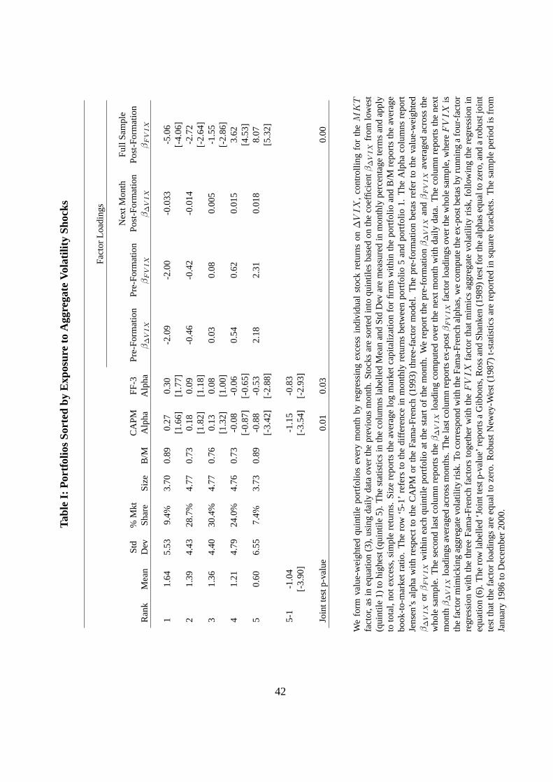
Tabl

eI:

Por

tfolio

sS

orte

dby

Exp

osur

eto

Agg

rega

teVo

latil

ityS

hock

s

Fac

tor

Load

ings

Nex

tMon

thF

ullS

ampl

eS

td%

Mkt

CA

PM

FF

-3P

re-F

orm

atio

nP

re-F

orm

atio

nP

ost-

For

mat

ion

Pos

t-F

orm

atio

nR

ank

Mea

nD

evS

hare

Siz

eB

/MA

lpha

Alp

haβ

∆V

IX

βF

VIX

β∆

VIX

βF

VIX

11.

645.

539.

4%3.

700.

890.

270.

30-2

.09

-2.0

0-0

.033

-5.0

6[1

.66]

[1.7

7][-

4.06

]2

1.39

4.43

28.7

%4.

770.

730.

180.

09-0

.46

-0.4

2-0

.014

-2.7

2[1

.82]

[1.1

8][-

2.64

]3

1.36

4.40

30.4

%4.

770.

760.

130.

080.

030.

080.

005

-1.5

5[1

.32]

[1.0

0][-

2.86

]4

1.21

4.79

24.0

%4.

760.

73-0

.08

-0.0

60.

540.

620.

015

3.62

[-0.

87]

[-0.

65]

[4.5

3]5

0.60

6.55

7.4%

3.73

0.89

-0.8

8-0

.53

2.18

2.31

0.01

88.

07[-

3.42

][-

2.88

][5

.32]

5-1

-1.0

4-1

.15

-0.8

3[-

3.90

][-

3.54

][-

2.93

]

Join

ttes

tp-v

alue

0.01

0.03

0.00

We

form

valu

e-w

eigh

ted

quin

tile

port

folio

sev

ery

mon

thby

regr

essi

ngex

cess

indi

vidu

alst

ock

retu

rns

on∆

VIX

,co

ntro

lling

for

theM

KT

fact

or,a

sin

equa

tion

(3),

usin

gda

ilyda

taov

erth

epr

evio

usm

onth

.S

tock

sar

eso

rted

into

quin

tiles

base

don

the

coef

ficie

ntβ

∆V

IX

from

low

est

(qui

ntile

1)to

high

est(

quin

tile

5).

The

stat

istic

sin

the

colu

mns

labe

lled

Mea

nan

dS

tdD

evar

em

easu

red

inm

onth

lype

rcen

tage

term

san

dap

ply

toto

tal,

note

xces

s,si

mpl

ere

turn

s.S

ize

repo

rts

the

aver

age

log

mar

ketc

apita

lizat

ion

for

firm

sw

ithin

the

port

folio

and

B/M

repo

rts

the

aver

age

book

-to-

mar

ket

ratio

.T

hero

w‘5

-1’r

efer

sto

the

diffe

renc

ein

mon

thly

retu

rns

betw

een

port

folio

5an

dpo

rtfo

lio1.

The

Alp

haco

lum

nsre

port

Jens

en’s

alph

aw

ithre

spec

tto

the

CA

PM

orth

eF

ama-

Fre

nch

(199

3)th

ree-

fact

orm

odel

.T

hepr

e-fo

rmat

ion

beta

sre

fer

toth

eva

lue-

wei

ghte

dβ

∆V

IX

orβ

FV

IX

with

inea

chqu

intil

epo

rtfo

lioat

the

star

toft

hem

onth

.W

ere

port

the

pre-

form

atio

nβ

∆V

IX

andβ

FV

IX

aver

aged

acro

ssth

ew

hole

sam

ple.

The

seco

ndla

stco

lum

nre

port

sth

eβ

∆V

IX

load

ing

com

pute

dov

erth

ene

xtm

onth

with

daily

data

.T

heco

lum

nre

port

sth

ene

xtm

onth

β∆

VIX

load

ings

aver

aged

acro

ssm

onth

s.T

hela

stco

lum

nre

port

sex

-pos

tβ

FV

IX

fact

orlo

adin

gsov

erth

ew

hole

sam

ple,

whe

reF

VIX

isth

efa

ctor

mim

icki

ngag

greg

ate

vola

tility

risk.

Toco

rres

pond

with

the

Fam

a-F

renc

hal

phas

,we

com

pute

the

ex-p

ostb

etas

byru

nnin

ga

four

-fac

tor

regr

essi

onw

ithth

eth

ree

Fam

a-F

renc

hfa

ctor

sto

geth

erw

ithth

eF

VIX

fact

orth

atm

imic

sag

greg

ate

vola

tility

risk,

follo

win

gth

ere

gres

sion

ineq

uatio

n(6

).T

hero

wla

belle

d‘J

oint

test

p-va

lue’

repo

rts

aG

ibbo

ns,R

oss

and

Sha

nken

(198

9)te

stfo

rth

eal

phas

equa

lto

zero

,and

aro

bust

join

tte

stth

atth

efa

ctor

load

ings

are

equa

lto

zero

.R

obus

tNew

ey-W

est(

1987

)t-

stat

istic

sar

ere

port

edin

squa

rebr

acke

ts.

The

sam

ple

perio

dis

from

Janu

ary

1986

toD

ecem

ber

2000

.

42

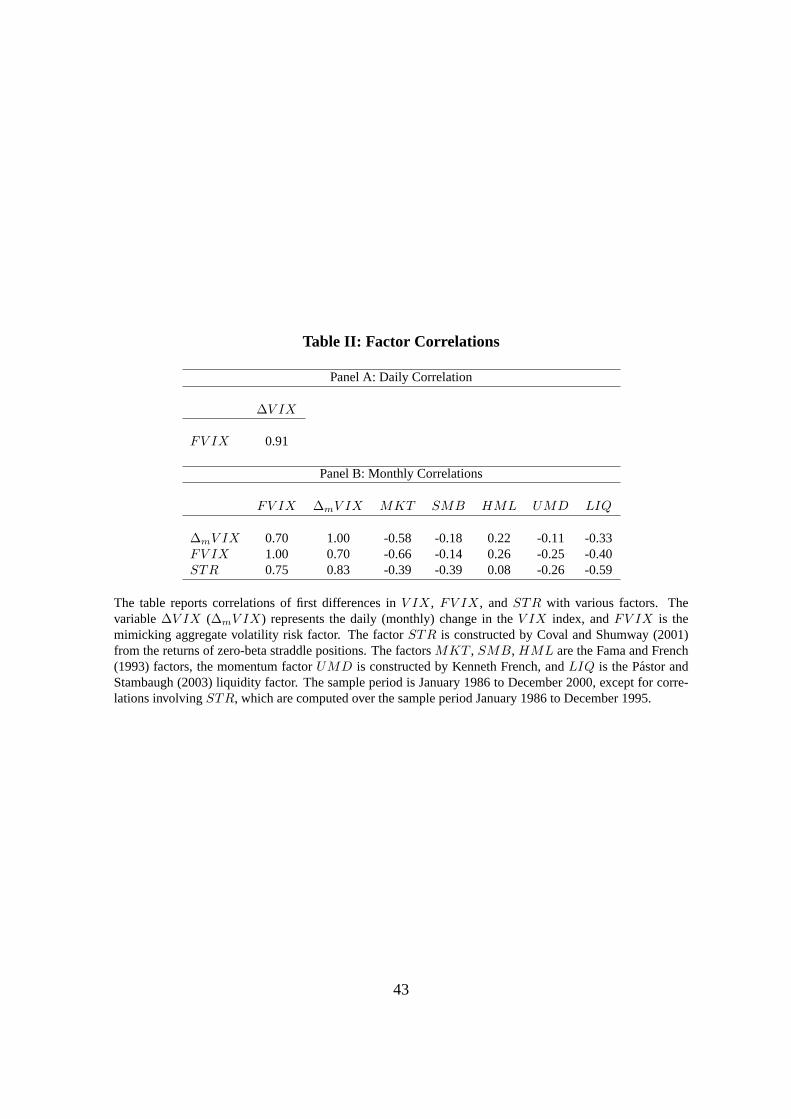
Table II: Factor Correlations

Panel A: Daily Correlation

∆V IX

FV IX 0.91

Panel B: Monthly Correlations

FV IX ∆mV IX MKT SMB HML UMD LIQ

∆mV IX 0.70 1.00 -0.58 -0.18 0.22 -0.11 -0.33FV IX 1.00 0.70 -0.66 -0.14 0.26 -0.25 -0.40STR 0.75 0.83 -0.39 -0.39 0.08 -0.26 -0.59

The table reports correlations of first differences inV IX, FV IX, andSTR with various factors. Thevariable∆V IX (∆mV IX) represents the daily (monthly) change in theV IX index, andFV IX is themimicking aggregate volatility risk factor. The factorSTR is constructed by Coval and Shumway (2001)from the returns of zero-beta straddle positions. The factorsMKT , SMB, HML are the Fama and French(1993) factors, the momentum factorUMD is constructed by Kenneth French, andLIQ is the Pastor andStambaugh (2003) liquidity factor. The sample period is January 1986 to December 2000, except for corre-lations involvingSTR, which are computed over the sample period January 1986 to December 1995.

43

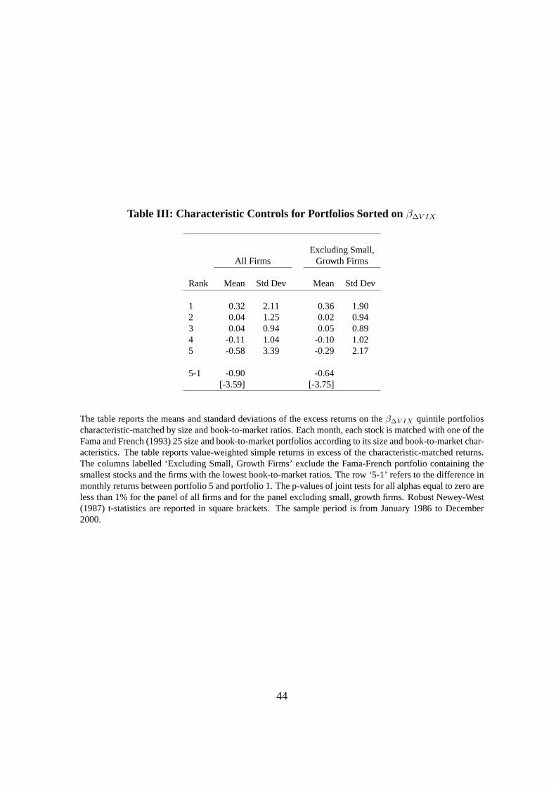
Table III: Characteristic Controls for Portfolios Sorted on β∆V IX

Excluding Small,All Firms Growth Firms

Rank Mean Std Dev Mean Std Dev

1 0.32 2.11 0.36 1.902 0.04 1.25 0.02 0.943 0.04 0.94 0.05 0.894 -0.11 1.04 -0.10 1.025 -0.58 3.39 -0.29 2.17

5-1 -0.90 -0.64[-3.59] [-3.75]

The table reports the means and standard deviations of the excess returns on theβ∆V IX quintile portfolioscharacteristic-matched by size and book-to-market ratios. Each month, each stock is matched with one of theFama and French (1993) 25 size and book-to-market portfolios according to its size and book-to-market char-acteristics. The table reports value-weighted simple returns in excess of the characteristic-matched returns.The columns labelled ‘Excluding Small, Growth Firms’ exclude the Fama-French portfolio containing thesmallest stocks and the firms with the lowest book-to-market ratios. The row ‘5-1’ refers to the difference inmonthly returns between portfolio 5 and portfolio 1. The p-values of joint tests for all alphas equal to zero areless than 1% for the panel of all firms and for the panel excluding small, growth firms. Robust Newey-West(1987) t-statistics are reported in square brackets. The sample period is from January 1986 to December2000.

44

Table IV: Portfolios Sorted on β∆V IX Controlling for Liquidity, Volume and Momentum

CAPM FF-3 Pre-Formation Post-FormationRank Mean Std Dev Alpha Alpha β∆V IX Loading βFV IX Loading

Panel A: Controlling for Liquidity

1 1.57 5.47 0.21 0.19 -1.89 -1.87[1.31] [1.34] [-1.65]

2 1.48 4.48 0.27 0.15 -0.43 -2.70[2.25] [1.68] [-2.78]

3 1.40 4.54 0.15 0.09 0.03 -1.34[1.59] [0.97] [-1.90]

4 1.30 4.74 0.02 -0.02 0.49 0.49[0.21] [-0.17] [0.54]

5 0.89 5.84 -0.52 -0.36 1.96 5.38[-2.87] [-2.09] [4.26]

5-1 -0.68 -0.73 -0.55[-3.04] [-2.99] [-2.15]

Joint test p-value 0.04 0.01 0.00

Panel B: Controlling for Volume

1 1.10 4.73 -0.11 -0.13 -2.08 -3.12[-0.58] [-1.34] [-3.17]

2 1.18 4.01 0.08 -0.08 -0.47 -3.39[0.46] [-0.92] [-4.19]

3 1.18 3.78 0.10 -0.04 0.04 -2.84[0.66] [-0.50] [-4.84]

4 0.98 4.18 -0.17 -0.23 0.55 0.14[-1.06] [2.16] [0.24]

5 0.38 5.31 -0.90 -0.71 2.17 4.29[-3.86] [-4.84] [5.07]

5-1 -0.72 -0.79 -0.58[-3.49] [-3.22] [-3.03]

Joint test p-value 0.00 0.00 0.00

45

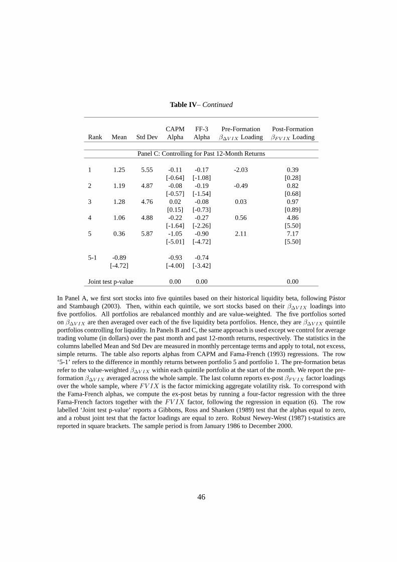
Table IV– Continued

CAPM FF-3 Pre-Formation Post-FormationRank Mean Std Dev Alpha Alpha β∆V IX Loading βFV IX Loading

Panel C: Controlling for Past 12-Month Returns

1 1.25 5.55 -0.11 -0.17 -2.03 0.39[-0.64] [-1.08] [0.28]

2 1.19 4.87 -0.08 -0.19 -0.49 0.82[-0.57] [-1.54] [0.68]

3 1.28 4.76 0.02 -0.08 0.03 0.97[0.15] [-0.73] [0.89]

4 1.06 4.88 -0.22 -0.27 0.56 4.86[-1.64] [-2.26] [5.50]

5 0.36 5.87 -1.05 -0.90 2.11 7.17[-5.01] [-4.72] [5.50]

5-1 -0.89 -0.93 -0.74[-4.72] [-4.00] [-3.42]

Joint test p-value 0.00 0.00 0.00

In Panel A, we first sort stocks into five quintiles based on their historical liquidity beta, following Pastorand Stambaugh (2003). Then, within each quintile, we sort stocks based on theirβ∆V IX loadings intofive portfolios. All portfolios are rebalanced monthly and are value-weighted. The five portfolios sortedon β∆V IX are then averaged over each of the five liquidity beta portfolios. Hence, they areβ∆V IX quintileportfolios controlling for liquidity. In Panels B and C, the same approach is used except we control for averagetrading volume (in dollars) over the past month and past 12-month returns, respectively. The statistics in thecolumns labelled Mean and Std Dev are measured in monthly percentage terms and apply to total, not excess,simple returns. The table also reports alphas from CAPM and Fama-French (1993) regressions. The row‘5-1’ refers to the difference in monthly returns between portfolio 5 and portfolio 1. The pre-formation betasrefer to the value-weightedβ∆V IX within each quintile portfolio at the start of the month. We report the pre-formationβ∆V IX averaged across the whole sample. The last column reports ex-postβFV IX factor loadingsover the whole sample, whereFV IX is the factor mimicking aggregate volatility risk. To correspond withthe Fama-French alphas, we compute the ex-post betas by running a four-factor regression with the threeFama-French factors together with theFV IX factor, following the regression in equation (6). The rowlabelled ‘Joint test p-value’ reports a Gibbons, Ross and Shanken (1989) test that the alphas equal to zero,and a robust joint test that the factor loadings are equal to zero. Robust Newey-West (1987) t-statistics arereported in square brackets. The sample period is from January 1986 to December 2000.

46

Table V: Estimating the Price of Volatility Risk

Panel A: Fama-MacBeth (1973) Factor Premiums

I II III IV

Constant -0.145 -0.527 -0.202 -0.247[-0.23] [-0.88] [-0.31] [-0.36]

MKT 0.977 1.276 1.034 1.042[1.11] [1.47] [1.13] [1.13]

FV IX -0.080 -0.082 -0.071[-2.49] [-2.39] [-2.02]

STR -0.194[-2.32]

SMB -0.638 -0.246 -0.608 -0.699[-1.24] [-0.59] [-1.13] [-1.25]

HML -0.590 -0.247 -0.533 -0.232[-0.95] [-0.40] [-0.82] [-0.34]

UMD 0.827 0.612[0.83] [0.59]

LIQ -0.021[-1.00]

Adj R2 0.67 0.56 0.65 0.79

Panel B: Ex-Post Factor Loadings onFV IX

Pre-ranking onβ∆V IX

1 low 2 3 4 5

Pre-ranking Low 1 -1.57 -5.89 -3.83 -3.35 -1.03onβMKT [-0.46] [-3.23] [-1.93] [-1.99] [-0.45]

2 -3.49 -4.47 -4.01 -2.00 -0.54[-1.67] [-3.18] [-3.11] [-1.66] [-0.31]

3 -5.74 -3.49 -2.56 -0.95 3.72[-3.16] [-2.84] [-2.21] [-0.78] [2.30]

4 -5.80 -1.41 -0.34 3.39 6.66[-4.13] [-1.00] [-0.29] [2.69] [3.85]

High 5 -3.69 -0.57 3.52 7.81 11.70[-2.05] [-0.45] [1.76] [3.32] [3.13]

Panel A reports the Fama-MacBeth (1973) factor premiums on 25 portfolios sorted first onβMKT and thenonβ∆V IX . MKT is the excess return on the market portfolio,FV IX is the mimicking factor for aggregatevolatility innovations,STR is Coval and Shumway’s (2001) zero-beta straddle return,SMB andHMLare the Fama-French (1993) size and value factors,UMD is the momentum factor constructed by KennethFrench, andLIQ is the aggregate liquidity measure from Pastor and Stambaugh (2003). In Panel B, we reportex-post factor loadings onFV IX, from the regression specification I (Fama-French model plusFV IX).Robust t-statistics that account for the errors-in-variables for the first-stage estimation in the factor loadingsare reported in square brackets. The sample period is from January 1986 to December 2000, except for theFama-MacBeth regressions withSTR, which are from January 1986 to December 1995.

47

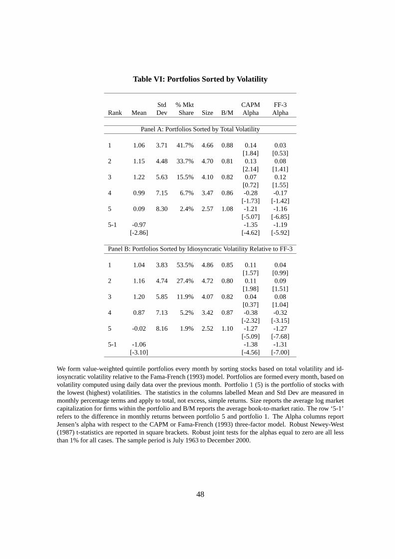
Table VI: Portfolios Sorted by Volatility

Std % Mkt CAPM FF-3Rank Mean Dev Share Size B/M Alpha Alpha

Panel A: Portfolios Sorted by Total Volatility

1 1.06 3.71 41.7% 4.66 0.88 0.14 0.03[1.84] [0.53]

2 1.15 4.48 33.7% 4.70 0.81 0.13 0.08[2.14] [1.41]

3 1.22 5.63 15.5% 4.10 0.82 0.07 0.12[0.72] [1.55]

4 0.99 7.15 6.7% 3.47 0.86 -0.28 -0.17[-1.73] [-1.42]

5 0.09 8.30 2.4% 2.57 1.08 -1.21 -1.16[-5.07] [-6.85]

5-1 -0.97 -1.35 -1.19[-2.86] [-4.62] [-5.92]

Panel B: Portfolios Sorted by Idiosyncratic Volatility Relative to FF-3

1 1.04 3.83 53.5% 4.86 0.85 0.11 0.04[1.57] [0.99]

2 1.16 4.74 27.4% 4.72 0.80 0.11 0.09[1.98] [1.51]

3 1.20 5.85 11.9% 4.07 0.82 0.04 0.08[0.37] [1.04]

4 0.87 7.13 5.2% 3.42 0.87 -0.38 -0.32[-2.32] [-3.15]

5 -0.02 8.16 1.9% 2.52 1.10 -1.27 -1.27[-5.09] [-7.68]

5-1 -1.06 -1.38 -1.31[-3.10] [-4.56] [-7.00]

We form value-weighted quintile portfolios every month by sorting stocks based on total volatility and id-iosyncratic volatility relative to the Fama-French (1993) model. Portfolios are formed every month, based onvolatility computed using daily data over the previous month. Portfolio 1 (5) is the portfolio of stocks withthe lowest (highest) volatilities. The statistics in the columns labelled Mean and Std Dev are measured inmonthly percentage terms and apply to total, not excess, simple returns. Size reports the average log marketcapitalization for firms within the portfolio and B/M reports the average book-to-market ratio. The row ‘5-1’refers to the difference in monthly returns between portfolio 5 and portfolio 1. The Alpha columns reportJensen’s alpha with respect to the CAPM or Fama-French (1993) three-factor model. Robust Newey-West(1987) t-statistics are reported in square brackets. Robust joint tests for the alphas equal to zero are all lessthan 1% for all cases. The sample period is July 1963 to December 2000.

48

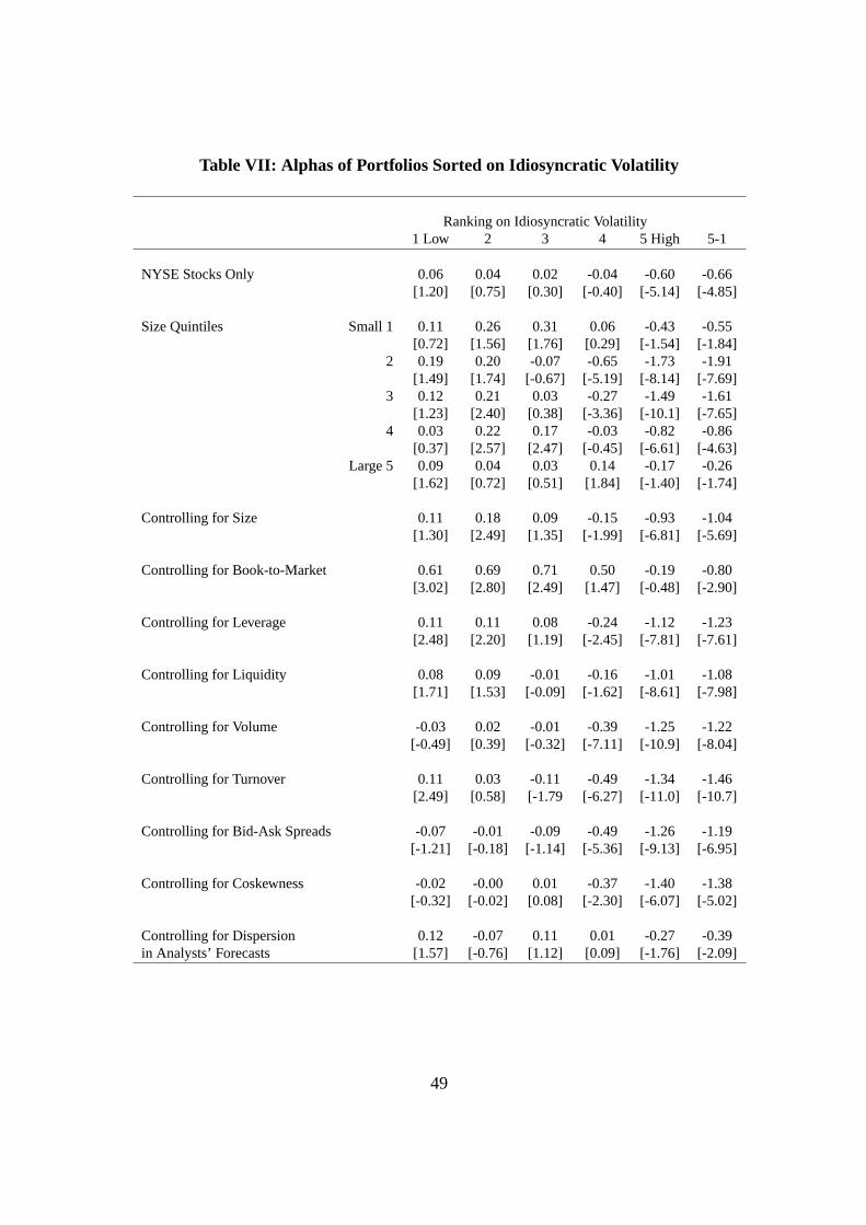
Table VII: Alphas of Portfolios Sorted on Idiosyncratic Volatility

Ranking on Idiosyncratic Volatility1 Low 2 3 4 5 High 5-1

NYSE Stocks Only 0.06 0.04 0.02 -0.04 -0.60 -0.66[1.20] [0.75] [0.30] [-0.40] [-5.14] [-4.85]

Size Quintiles Small 1 0.11 0.26 0.31 0.06 -0.43 -0.55[0.72] [1.56] [1.76] [0.29] [-1.54] [-1.84]

2 0.19 0.20 -0.07 -0.65 -1.73 -1.91[1.49] [1.74] [-0.67] [-5.19] [-8.14] [-7.69]

3 0.12 0.21 0.03 -0.27 -1.49 -1.61[1.23] [2.40] [0.38] [-3.36] [-10.1] [-7.65]

4 0.03 0.22 0.17 -0.03 -0.82 -0.86[0.37] [2.57] [2.47] [-0.45] [-6.61] [-4.63]

Large 5 0.09 0.04 0.03 0.14 -0.17 -0.26[1.62] [0.72] [0.51] [1.84] [-1.40] [-1.74]

Controlling for Size 0.11 0.18 0.09 -0.15 -0.93 -1.04[1.30] [2.49] [1.35] [-1.99] [-6.81] [-5.69]

Controlling for Book-to-Market 0.61 0.69 0.71 0.50 -0.19 -0.80[3.02] [2.80] [2.49] [1.47] [-0.48] [-2.90]

Controlling for Leverage 0.11 0.11 0.08 -0.24 -1.12 -1.23[2.48] [2.20] [1.19] [-2.45] [-7.81] [-7.61]

Controlling for Liquidity 0.08 0.09 -0.01 -0.16 -1.01 -1.08[1.71] [1.53] [-0.09] [-1.62] [-8.61] [-7.98]

Controlling for Volume -0.03 0.02 -0.01 -0.39 -1.25 -1.22[-0.49] [0.39] [-0.32] [-7.11] [-10.9] [-8.04]

Controlling for Turnover 0.11 0.03 -0.11 -0.49 -1.34 -1.46[2.49] [0.58] [-1.79 [-6.27] [-11.0] [-10.7]

Controlling for Bid-Ask Spreads -0.07 -0.01 -0.09 -0.49 -1.26 -1.19[-1.21] [-0.18] [-1.14] [-5.36] [-9.13] [-6.95]

Controlling for Coskewness -0.02 -0.00 0.01 -0.37 -1.40 -1.38[-0.32] [-0.02] [0.08] [-2.30] [-6.07] [-5.02]

Controlling for Dispersion 0.12 -0.07 0.11 0.01 -0.27 -0.39in Analysts’ Forecasts [1.57] [-0.76] [1.12] [0.09] [-1.76] [-2.09]

49

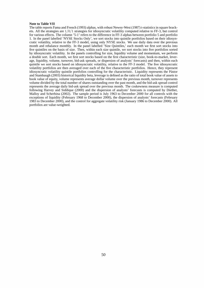
Note to Table VIIThe table reports Fama and French (1993) alphas, with robust Newey-West (1987) t-statistics in square brack-ets. All the strategies are1/0/1 strategies for idiosyncratic volatility computed relative to FF-3, but controlfor various effects. The column ’5-1’ refers to the difference in FF-3 alphas between portfolio 5 and portfolio1. In the panel labelled ’NYSE Stocks Only’, we sort stocks into quintile portfolios based on their idiosyn-cratic volatility, relative to the FF-3 model, using only NYSE stocks. We use daily data over the previousmonth and rebalance monthly. In the panel labelled ’Size Quintiles,’ each month we first sort stocks intofive quintiles on the basis of size. Then, within each size quintile, we sort stocks into five portfolios sortedby idiosyncratic volatility. In the panels controlling for size, liquidity volume and momentum, we performa double sort. Each month, we first sort stocks based on the first characteristic (size, book-to-market, lever-age, liquidity, volume, turnover, bid-ask spreads, or dispersion of analysts’ forecasts) and then, within eachquintile we sort stocks based on idiosyncratic volatility, relative to the FF-3 model. The five idiosyncraticvolatility portfolios are then averaged over each of the five characteristic portfolios. Hence, they representidiosyncratic volatility quintile portfolios controlling for the characteristic. Liquidity represents the Pastorand Stambaugh (2003) historical liquidity beta, leverage is defined as the ratio of total book value of assets tobook value of equity, volume represents average dollar volume over the previous month, turnover representsvolume divided by the total number of shares outstanding over the past month, and the bid-ask spread controlrepresents the average daily bid-ask spread over the previous month. The coskewness measure is computedfollowing Harvey and Siddique (2000) and the dispersion of analysts’ forecasts is computed by Diether,Malloy and Scherbina (2002). The sample period is July 1963 to December 2000 for all controls with theexceptions of liquidity (February 1968 to December 2000), the dispersion of analysts’ forecasts (February1983 to December 2000), and the control for aggregate volatility risk (January 1986 to December 2000). Allportfolios are value-weighted.

50

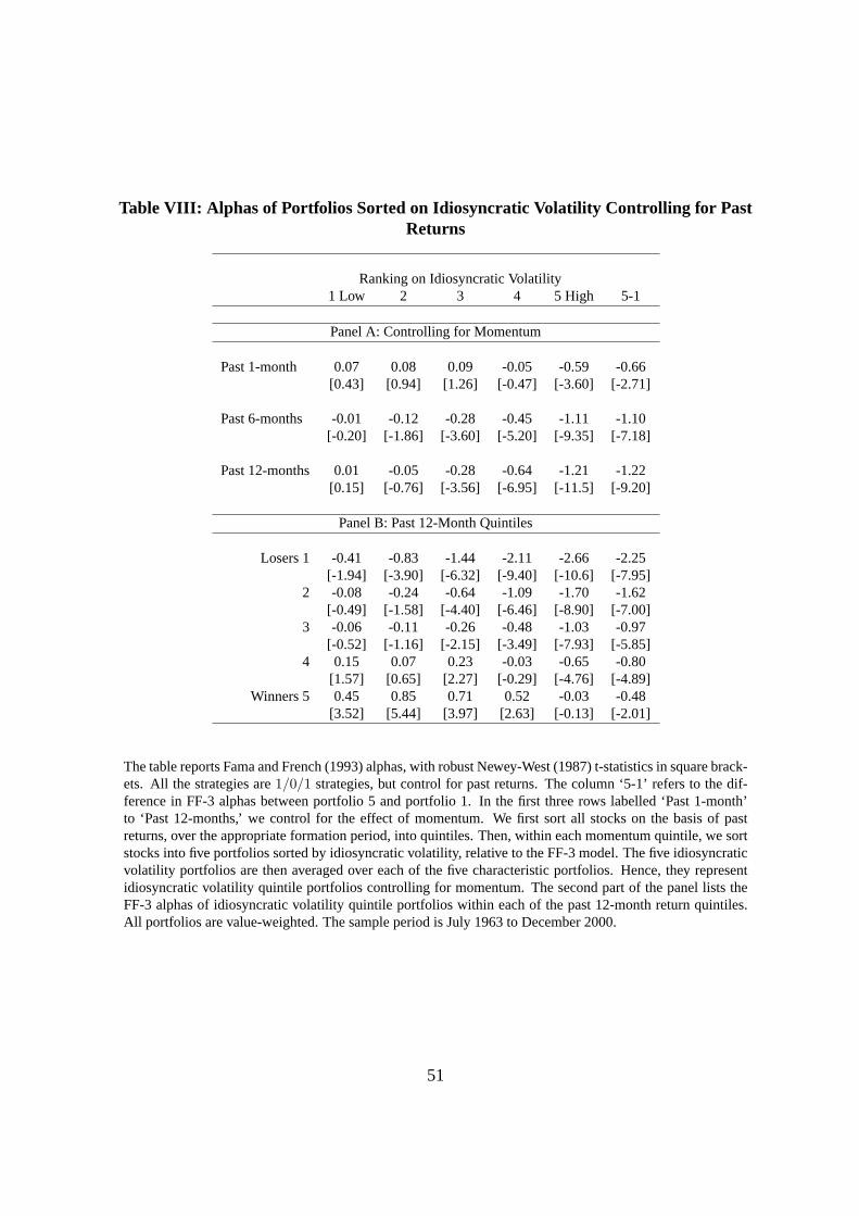
Table VIII: Alphas of Portfolios Sorted on Idiosyncratic Volatility Controlling for PastReturns

Ranking on Idiosyncratic Volatility1 Low 2 3 4 5 High 5-1

Panel A: Controlling for Momentum

Past 1-month 0.07 0.08 0.09 -0.05 -0.59 -0.66[0.43] [0.94] [1.26] [-0.47] [-3.60] [-2.71]

Past 6-months -0.01 -0.12 -0.28 -0.45 -1.11 -1.10[-0.20] [-1.86] [-3.60] [-5.20] [-9.35] [-7.18]

Past 12-months 0.01 -0.05 -0.28 -0.64 -1.21 -1.22[0.15] [-0.76] [-3.56] [-6.95] [-11.5] [-9.20]

Panel B: Past 12-Month Quintiles

Losers 1 -0.41 -0.83 -1.44 -2.11 -2.66 -2.25[-1.94] [-3.90] [-6.32] [-9.40] [-10.6] [-7.95]

2 -0.08 -0.24 -0.64 -1.09 -1.70 -1.62[-0.49] [-1.58] [-4.40] [-6.46] [-8.90] [-7.00]

3 -0.06 -0.11 -0.26 -0.48 -1.03 -0.97[-0.52] [-1.16] [-2.15] [-3.49] [-7.93] [-5.85]

4 0.15 0.07 0.23 -0.03 -0.65 -0.80[1.57] [0.65] [2.27] [-0.29] [-4.76] [-4.89]

Winners 5 0.45 0.85 0.71 0.52 -0.03 -0.48[3.52] [5.44] [3.97] [2.63] [-0.13] [-2.01]

The table reports Fama and French (1993) alphas, with robust Newey-West (1987) t-statistics in square brack-ets. All the strategies are1/0/1 strategies, but control for past returns. The column ‘5-1’ refers to the dif-ference in FF-3 alphas between portfolio 5 and portfolio 1. In the first three rows labelled ‘Past 1-month’to ‘Past 12-months,’ we control for the effect of momentum. We first sort all stocks on the basis of pastreturns, over the appropriate formation period, into quintiles. Then, within each momentum quintile, we sortstocks into five portfolios sorted by idiosyncratic volatility, relative to the FF-3 model. The five idiosyncraticvolatility portfolios are then averaged over each of the five characteristic portfolios. Hence, they representidiosyncratic volatility quintile portfolios controlling for momentum. The second part of the panel lists theFF-3 alphas of idiosyncratic volatility quintile portfolios within each of the past 12-month return quintiles.All portfolios are value-weighted. The sample period is July 1963 to December 2000.

51

Table IX: The Idiosyncratic Volatility Effect Controlling for Aggregate Volatility Risk

Ranking on Idiosyncratic Volatility1 Low 2 3 4 5 High 5-1

Panel A: FF-3 Alphas

Controlling for Exposure to 0.05 0.01 -0.14 -0.49 -1.14 -1.19Aggregate Volatility Risk [0.83] [0.09] [-1.14] [-3.08] [-5.00] [-4.72]

Panel B:FV IX Factor Loadings

β∆V IX Quintiles Low 1 -6.40 -1.98 -0.55 8.80 7.51[-3.82] [-0.78] [-0.23] [2.16] [2.31]

2 -2.66 -3.21 0.06 -3.04 5.37[-2.27] [-2.06] [0.05] [-2.00] [1.80]

3 -6.51 -2.74 -1.93 -0.31 7.25[-4.50] [-2.41] [-1.14] [-0.29] [3.37]

4 5.65 3.73 3.50 1.33 8.22[2.31] [2.08] [2.83] [0.87] [3.97]

High 5 7.53 2.46 8.60 7.53 5.79[5.16] [1.16] [3.72] [2.53] [1.65]

We control for exposure to aggregate volatility using theβ∆V IX loading at the beginning of the month,computed using daily data over the previous month, following equation (3). We first sort all stocks on thebasis ofβ∆V IX into quintiles. Then, within eachβ∆V IX quintile, we sort stocks into five portfolios sortedby idiosyncratic volatility, relative to the FF-3 model. In Panel A, we report FF-3 alphas of these portfolios.We average the five idiosyncratic volatility portfolios over each of the fiveβ∆V IX portfolios. Hence, theseportfolios represent idiosyncratic volatility quintile portfolios controlling for exposure to aggregate volatilityrisk. The column ‘5-1’ refers to the difference in FF-3 alphas between portfolio 5 and portfolio 1. In Panel B,we report ex-postFV IX factor loadings from a regression of each of the 25β∆V IX× idiosyncratic volatilityportfolios onto the Fama-French (1993) model augmented withFV IX as in equation (6). Robust Newey-West (1987) t-statistics are reported in square brackets. All portfolios are value-weighted. The sample periodis from January 1986 to December 2000.

52

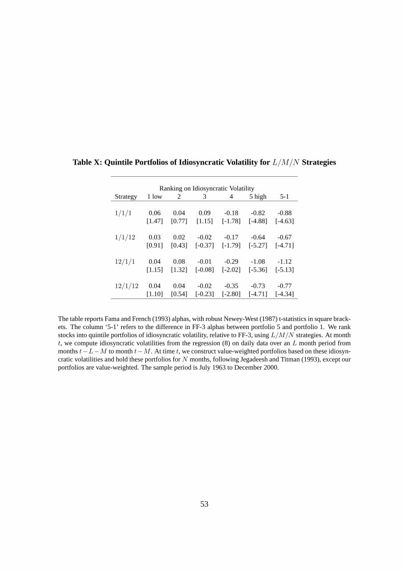
Table X: Quintile Portfolios of Idiosyncratic Volatility for L/M/N Strategies

Ranking on Idiosyncratic VolatilityStrategy 1 low 2 3 4 5 high 5-1

1/1/1 0.06 0.04 0.09 -0.18 -0.82 -0.88[1.47] [0.77] [1.15] [-1.78] [-4.88] [-4.63]

1/1/12 0.03 0.02 -0.02 -0.17 -0.64 -0.67[0.91] [0.43] [-0.37] [-1.79] [-5.27] [-4.71]

12/1/1 0.04 0.08 -0.01 -0.29 -1.08 -1.12[1.15] [1.32] [-0.08] [-2.02] [-5.36] [-5.13]

12/1/12 0.04 0.04 -0.02 -0.35 -0.73 -0.77[1.10] [0.54] [-0.23] [-2.80] [-4.71] [-4.34]

The table reports Fama and French (1993) alphas, with robust Newey-West (1987) t-statistics in square brack-ets. The column ‘5-1’ refers to the difference in FF-3 alphas between portfolio 5 and portfolio 1. We rankstocks into quintile portfolios of idiosyncratic volatility, relative to FF-3, usingL/M/N strategies. At montht, we compute idiosyncratic volatilities from the regression (8) on daily data over anL month period frommonthst−L−M to montht−M . At time t, we construct value-weighted portfolios based on these idiosyn-cratic volatilities and hold these portfolios forN months, following Jegadeesh and Titman (1993), except ourportfolios are value-weighted. The sample period is July 1963 to December 2000.

53

Table XI: The Idiosyncratic Volatility Effect over Different Subsamples

Ranking on Idiosyncratic VolatilitySubperiod 1 low 2 3 4 5 high 5-1

Jul 1963 – Dec 1970 0.06 0.03 0.09 -0.36 -0.94 -1.00[1.23] [0.42] [0.73] [-2.18] [-5.81] [-5.62]

Jan 1971 – Dec 1980 -0.24 0.32 0.19 0.03 -1.02 -0.77[-2.53] [3.20] [1.55] [0.21] [-5.80] [-3.14]

Jan 1981 – Dec 1990 0.15 0.08 -0.16 -0.66 -2.08 -2.23[2.14] [1.07] [-1.25] [-4.82] [-10.1] [-9.39]

Jan 1991 – Dec 2000 0.16 -0.01 0.14 -0.48 -1.39 -1.55[1.34] [-0.08] [0.77] [-2.41] [-3.31] [-3.19]

NBER Expansions 0.06 0.02 0.08 -0.33 -1.19 -1.25[1.26] [0.25] [1.01] [-3.18] [-7.07] [-6.55]

NBER Recessions -0.10 0.64 -0.01 -0.34 -1.88 -1.79[-0.65] [3.58] [-0.04] [-1.32] [-3.32] [-2.63]

Stable Periods 0.05 -0.02 -0.11 -0.62 -1.66 -1.71[0.44] [-0.25] [-1.07] [-4.06] [-6.56] [-4.75]

Volatile Periods -0.04 0.24 0.32 0.18 -0.93 -0.89[-0.29] [1.69] [2.32] [0.55] [-2.40] [-2.02]

The table reports Fama and French (1993) alphas, with robust Newey-West (1987) t-statistics in square brack-ets. The column ‘5-1’ refers to the difference in FF-3 alphas between portfolio 5 and portfolio 1. We rankstocks into quintile portfolios of idiosyncratic volatility, relative to FF-3, using the1/0/1 strategy and ex-amine robustness over different sample periods. The stable and volatile periods refer to the months with thelowest and highest 20% absolute value of the market return, respectively. The full sample period is July 1963to December 2000.

54

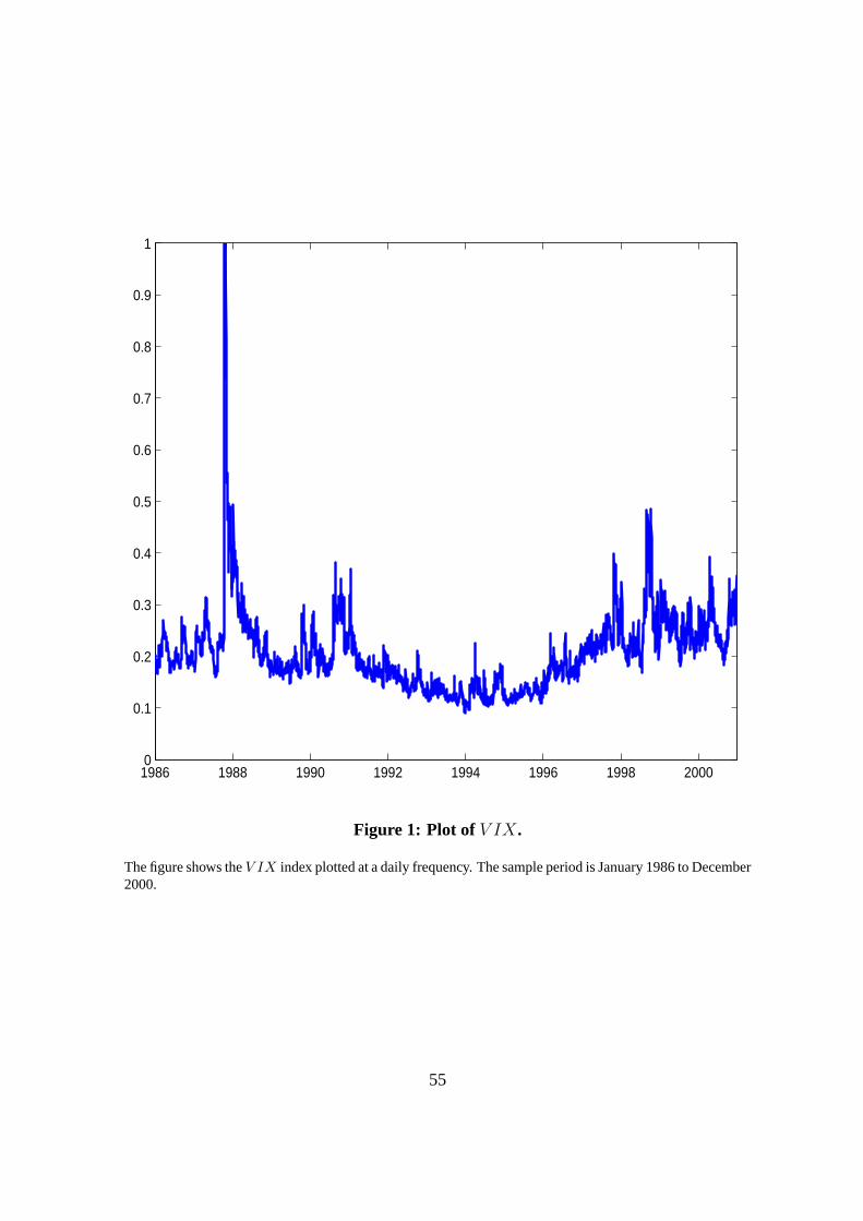
1986 1988 1990 1992 1994 1996 1998 20000

0.1

0.2

0.3

0.4

0.5

0.6

0.7

0.8

0.9

1

Figure 1: Plot of V IX.

The figure shows theV IX index plotted at a daily frequency. The sample period is January 1986 to December2000.

55