Expected Stock Returns and Earnings Volatility∗

Alan Guoming Huang†

December 15, 2004

∗Preliminary. Comments welcome.†Department of Finance, Leeds School of Business, University of Colorado, Boulder, CO 80309, email:

guoming.huang@colorado.edu, tel: 303-492-4405. I thank Boochun Jung, Kevin Sun, Sunny Yang, JaimeZender, and in particular my advisors Eric Hughson and Chris Leach for many helpful discussions andcomments. I am solely responsible for all errors.

Abstract

In an economy with short-lived investors and a finite number of firms, firms with

more volatile earnings are assigned lower prices in equilibrium. This finding suggests

that earnings volatility should be a factor in determining expected stock returns, other

things being equal. We investigate the way earnings volatility interacts with traditional

factors for asset pricing.

We use multi-factor models to test whether earnings volatility helps explain the

cross section of stock returns. We find that earnings volatility, as measured by the

coefficient of variation of earnings or cashflow, loads positively in panel and time-series

regressions of size-sorted portfolio returns. However, it is not significant in cross-

sectional regressions of individual stock returns.

At the portfolio level, earnings volatility is significant in combination with a market

factor, and in combination with market, size, earnings yield, and book-to-market equity

most of the time. The loadings of earning volatility are robust across proxies for size

and earnings, windows for earnings volatility estimation, sub-samples, and sub-periods.

We are able to disentangle the earnings volatility factor from the size effect, but not

from return volatility. By constructing a mimicking portfolio for earnings volatility in

addition to Fama and French’s (1993) size and value mimicking portfolios, we find that

the earnings volatility factor almost always loads positively in time-series regressions

of stock returns. Depending on the proxy for earnings volatility, adding a return

volatility factor to multi-factor regressions may or may not deplete the explanatory

power of earnings volatility.

At the individual firm level, we do not find significance in earnings volatility in

Fama and French (1992) cross-sectional regressions of individual stock returns on beta,

size, book-to-market, and earning volatility. To account for the difference of earnings

volatility in explaining individual and portfolio returns, we conjecture that individual

earning volatility might be measured with error, or that earnings volatility is diversi-

fiable at the firm level but not at the portfolio level.

2

1 Introduction

Large amount of empirical evidence has linked cross-sectional stock returns to firm character-

istics, such as earning yield [e.g., Lamont (1998)], market equity, book-to-market ratio [e.g.,

Fama and French (1992), (1993)], dividend, and dividend payout ratio [e.g., Chen (1991),

Lettau and Ludvigson (2001)]. These relationships are hard to explain in the traditional

asset pricing paradigm; yet their loadings on returns are non-trivial. For example, Fama and

French (1992) document that size and book-to-market ratio alone account for cross-sectional

returns associated with the market beta.

Despite the empirical success of these firm characteristics in explaining returns, these as-

set pricing “anomalies” typically focus on the direct relationship between the level of variables

and stock returns. Much less attention has been paid to the possibility that the variability of

firm characteristics might affect returns. Of particular interest is earnings volatility, which

may have generic return implications given investors’ and managers’ apparent emphasis on

earnings. For example, Berk (1995) reasons that the size effect (that returns on small stocks

are higher than returns on large stocks) is due to firm cashflow riskiness, because the cor-

relation of cashflows with the underlying risk factors will vary across firms in a one-period

economy. There are also indirect evidence suggesting that earnings volatility may matter to

returns. For example, Badrinath, Gay and Kale (1989) find that institutional investors are

reluctant to invest companies with a history of large variations in earnings. Bricker et al.

(1995) report that analysts tend to avoid firms with volatile earnings for the fear of forecast

errors.

This paper investigates the relationship between earnings volatility and expected stock

returns. We first propose a parsimonious model with short-lived investors and limited number

of securities to show that there exists a negative relationship between earnings volatility

and price. In our multi-period, overlapping-generations (OLG) model, investors regard their

investment problem as a tradeoff between immediate consumption and savings by investing in

multiple assets that differ in dividend volatility. One advantage of using such a model is that

the volatility of an asset’s residual claims can be numerically linked to the certainty equivalent

of consumer’s utility for direct pricing purposes. Recent applications of OLG models by

Constantinides, Donaldson and Mehra (2002) and Huang, Hughson and Leach (2004) in

solving the equity premium puzzle show that asset returns can be expressed as the earnings

yield in the stationary equilibrium. This is achieved without turning to additionally imposed

1

structures such as log-normality assumption between returns and aggregate consumption,

which prior consumption-based CAPM models [e.g., Singleton and Hansen (1982), Campbell

and Cochrane (1999)] typically feature. When calibrating the model to historical income and

market data, we show that in equilibrium the cross-sectional variation in stocks’ earnings

volatility can be used to explain the cross-sectional variation in prices. A firm with a more

volatile cashflow stream is assigned lower price because of smaller certainty equivalent of

its cashflow; therefore, its market value is comparatively smaller while its earnings yield, or

return, is comparatively higher.

The economy we use to show the negative relationship between price and earnings volatil-

ity is one that a finite number of firms have independently distributed earnings. Although

not replicating the whole set of individual firms in the economy, it closely resembles the

situation that firms are aggregated into a limited number of portfolios, a situation that nu-

merous empirical asset pricing tests rest upon. Therefore, our results suggest that earnings

volatility should be a factor in determining expected stock returns, other things being equal.

Recent advancements in empirical asset pricing that idiosyncratic return volatility ex-

hibits predictive power on stock returns [e.g., Malkiel and Xu (2001), Guo and Savichas

(2003)] lend support to our thesis that earnings volatility might matter cross-sectionally.

There are several reasons why idiosyncratic risk, whether from earnings or returns, may be

priced. First, as argued by Malkiel and Xu (2001) and Levy (1978), many investors hold

poorly diversified portfolios. Second, market may be inefficient in that earing volatility is

firm-specific, fully diversifiable risk but investors incorrectly perceive it as priced, systematic

risk. Third and most important, CAPM may be misspecified and does not correctly price all

relevant factors, as it only holds under strict conditions, such as quadratic utility function

and constant investment opportunities.

Given that we argue for a story of earnings volatility, we next investigate the way earnings

volatility interacts with traditional factors for asset pricing. In particular, we are interested

in answering two empirical questions: (1) Can earnings volatility predict returns cross-

sectionally? And if the answer to (1) is positive, then (2) can earnings volatility serve as an

independent factor? Specifically, will earnings volatility be driven out with the presence of

return-informative variables such as size, book-to-market equity, earnings yield, and return

volatility, or the other way around?

To the best of our knowledge the empirical question of the volatility of corporate earnings

2

on returns hasn’t been answered. Prior studies on return prediction using historical earnings

focus on the level of earnings, such as earnings yield or dividend payout ratio [e.g., Fama

and French (1988), Lamont (1998), Lettau and Ludvigson (2001)]. In recent accounting

literature, Barnes (1999), and Allayannis and Weston (2003) both document that earnings

(cashflow) volatility is negatively related with market value, and therefore, managers have

incentives to smooth earnings over time. In light of these findings and our calibration

results, answering the empirical question of earnings volatility on returns contributes to

the identification of relevant pricing factors and motivates us to further refine asset pricing

theories.

We test the hypothesis that earnings volatility explains the cross section of stock returns

at both the portfolio level and the individual firm level. We adopt standard methodologies of

Fama and French (1993) to run time-series regressions on size-sorted portfolio returns, and

of Fama and French (1992) to run cross-sectional regressions on individual stock returns.

In addition to these standard regressions, we run panel regressions of returns based on the

perception that returns of multiple assets across time consist exactly of a panel data. Running

a panel regression is in line with the spirit of the two-pass regressions adopted in Fama and

MacBeth (1973) and Fama and French (1992), where the authors test the significance of

time-series coefficients of cross-sectional regressions. Directly applying a panel regression,

however, not only enables us to derive the exact significance level of the coefficients, but also

allows for different or unknown structures in the residuals, such as heteroscedascitiy and

auto-correlation.

At the portfolio level, to test the predictive power of earnings volatility on expected stock

returns, we regress size-sorted portfolio returns on multiple variables including earnings

volatility. We find that earnings volatility, as measured by the coefficient of variation of

earnings or cashflow (the standard deviation divided by the absolute mean) loads positively

in panel regressions of returns. Earnings volatility is significant at 1% in combination with

a market factor, and at 5% in combination with market, size, earnings yield, and book-to-

market equity most of the time. The R2s of these regressions are generally in the range

of 50-60%, which are comparable to those of Fama-French’s (1993) three-factor time-series

regressions. We use book equity sorted portfolios as the benchmark. However, the results are

robust to portfolios sorted on different size proxies, including market equity, total assets and

sales. The results are also robust across windows for earnings volatility estimation (e.g., using

past twelve quarters of earnings vs. sixteen quarters to estimate earnings volatility), proxies

3

for earnings volatility (e.g., standard deviation of earnings scaled by sales), sub-samples (e.g.,

NYSE stocks only), and sub-periods.

We are able to disentangle the earnings volatility factor at the portfolio level from the

size and value effects, but not from return volatility. We construct a mimicking portfolio of

earnings volatility in addition to Fama and French’s (1993) size and value mimicking portfo-

lios. We find that the earning volatility mimicking portfolio almost always loads positively

in time-series regressions of stock returns. However, the earnings volatility factor drives

out neither SMB, the size factor, nor HML, the value factor. Depending on the proxy

for earnings volatility, adding return volatility to a multi-factor regression may or may not

deplete the explanatory power of earnings volatility. We conclude that earnings volatility is

a pricing factor independent of market, earnings yield, size, and book-to-market equity. The

relationship between earnings volatility and return volatility seems worth further study.

At the individual firm level, we follow Fama and French (1992) and run cross-sectional

regressions of stock returns on β, size, book-to-market equity, and earning volatility. The

results, however, do not show evidence that earnings volatility contains return relevant infor-

mation. There are several possible reasons for the seemingly contradictory results between

the portfolio level and the individual firm level. It might be errors-in-variable problem for

earnings volatility at both the firm and portfolio levels, or that the portfolio level results

are simply sampling luck. Given firm accounting distortions, firm-specific shocks, and our

extensive robustness checks at the portfolio level, we are biased towards earnings volatility

predicts portfolio returns. Another reason might be that earnings volatility is diversifiable

at the firm level but not at the portfolio level. As shown in our calibration, when each port-

folio contributes significantly to the market portfolio, changes in portfolio earnings volatility

affect the market pricing kernel. If the market portfolio does not adjust fast enough or is

measured with error, portfolio earnings volatility will be priced. That said, how to reconcile

the difference in the explanatory power of earnings volatility between the portfolio level and

the individual level merits further study.

The rest of the paper is organized as follows. Section 2 presents and calibrates the model,

and shows that there is a negative relationship between earnings volatility and price when

the economy has a finite number of securities. Section 3 develops a factor representation

for the model and specifies the empirical tests. Section 4 describes the data and variables.

Section 5 details the empirical results at the portfolio level. Section 6 provides the results of

individual return regressions in the fashion of Fama and French (1992). Section 7 concludes.

4

2 Motivation: A Modelling Perspective

In this section we numerically show that in a parsimonious economy with a finite number

of firms, the general equilibrium implies that earnings volatility is negatively priced. The

economy used in the calibration closely resembles the one studied by Huang, Hughson and

Leach (2004, “HHL”). To foreshadow the results, other things being equal, in equilibrium

firm prices decrease with volatile earnings, as measured by the coefficient of variation of

earnings.

The calibration results may appear somewhat unorthodox within the traditional asset

pricing paradigm, where it is asserted that risk-adjusted returns should not include returns

from idiosyncratic risks such as earnings volatility. We argue for the pricing of earnings

volatility, for the reason that each asset in the economy contributes significantly to the

market portfolio when the number of securities is limited. In the words of CAPM, each asset

affects the market portfolio in a non-trivial way through (partially) independent earnings

components, so that earnings volatility is priced. Due to computational constraints, we are

not able to extend the calibration to a very large number of assets. Shall we be able to do

so, where individual assets is consider marginal against the market portfolio, we conjecture

that the traditional CAPM results will hold.

2.1 Short-lived investors and investment opportunities

Consider short-lived investors with stochastic investment opportunities. For simplicity, in-

vestors live for two periods. A generation t investor (consumer) is born young at time t,

grows old at time (t + 1), and ceases to exist at time (t + 2). The population consists of a

sufficiently large measure of two generations. Agents within each cohort are homogeneous

and rational. We can therefore construct a representative agent for each generation to study

the equilibrium. A generation t agent receives sequential wealth endowments w1 and w2,

and leaves no bequest or debt when he dies. w1 and w2 are assumed to be non-stochastic

for simplicity. There is only one numeraire consumption good in the economy. Agents in

generation-t choose security holdings to maximize a well-behaved, time-additive CRRA ex-

pected utility function: E[ 11−γ

∑1j=0 βj(Ct

t+j)1−γ], where Ct

t+j denotes the consumption by

generation t at time t+ j, γ is the relative risk aversion coefficient (RRA), and β is the time

preference factor.

5

In each period, there are N perfectly divisible securities indexed by 1, 2, ..., N . The

supply of each security is fixed at 1. A time-t investment in security i entitles the owner

to the resell price and the residual claim di (dividend/profit) at time t + 1. For illustrative

purposes, we assume that the dividend (profit) distributions of securities are IID cross-

sectionally and intertemporally, and follow normal distribution characterized by mean E(di)

and standard deviation σ(di) ∀ i. Let pit be the ex-dividend price of security i at t.

Constantanides, Donaldson and Mehra (2002), and HHL develop similar overlapping-

generations models to study the equity premium puzzle. The existence of a stationary

equilibrium, like one in Lucas (1978), has been proved in those papers. The conditional

equilibrium pricing equation for asset i is qualitatively identical with that in the standard

intertemporal CAPM:

Et[Mt+1Rit+1] = 1, (1)

where Mt+1 =Ct

t+1

Ct

t

−γ

, and Rit+1 =

pi

t+1+di

t+1

pi

t

. Note that Ctt+1 and Ct

t are derived consumptions

with budget conditions set at equality and market clearing conditions satisfied, i.e.,

Ctt = w1 −

∑

i

pit, (2)

and

Ctt+1 = w2 +

∑

i

(pit+1 + di

t+1). (3)

Also note that in stationary equilibrium, pit+1 = pi

t so that Rit+1 = 1 +

di

t+1

pi

t

.

2.2 Calibration

Equations (1)-(3) establish a system which exactly identifies the solution for unknown price

vector. However, for a reasonable positive value of γ, the pricing equations are highly non-

linear, for which an analytical solution is hard to solicit. To get around this, researchers

since Hansen and Singleton (1982) typically assume joint lognormality between equilibrium

consumption stream and returns, which conveniently transforms equation (1) to a linear

combination of γ and the covariance between consumption growth and returns. However,

given that consumption growth is too smooth to produce significant co-movements with

asset returns, this linear transformation is well known for its inability to explain the equity

6

premium [e.g., Mehra and Prescott (1985)] and other pricing anomalies such as the size and

value effects [e.g., Fama and French (1992)].

In the absence of analytical solution and the presence of potentially flawed transformation,

we turn to numerical solution and calibrate the economy. One advantage of a such method is

that each solution represents an equilibrium. We follow the line of HHL’s parameterization

of an OLG economy for calibration inputs.

We need input values for length (number of years) of each model period, w1, w2, γ,

β, securities number and their respective dividend distribution. In HHL, length of each

model period is set to be 25 years, that is, investors live for 50 years of economic life. Due

to the homogeneity property of the CRRA utility function [e.g., Constantnides, Donaldson

and Mehra (2002)], the solutions for returns in equations (1)-(3) are scale invariant. This

property enables us to conveniently normalize aggregate endowment to 1. The empirical

humped-shape life-time income profile [e.g., Attanasio (1998)] leads Auerbach and Kotlikoff

(1987) and others to adopt w(a) = exp(4.47 + 0.033a − 0.00067a2) for the representation

of income profile, where a is the number of years into earnings. Using this income profile

and assigning the first (second) half of lifetime income to w1 (w2) result in w1 = 0.507

and w2 = 0.493. We set γ to 6. Choosing a single-digit γ is consistent with the existing

empirical evidence that the population-wide risk aversion coefficient is generally less than 10

[e.g., Barsky et al. (1997), Chetty (2003)] and avoids the equity premium puzzle problem.

As for the rate of time preference, β, most economists agree that it should be less than 1.

We use HHL’s value of 0.99. In unreported sensitivity analysis, both higher γ and lower β

increase the price differentials between assets with different earnings volatilities; however,

they don’t change the nature of the model predictions. Model period returns are converted

into annualized returns using simple annualization, as with HHL. Returns are then reported

in the annual basis. In summary, we use the following inputs for the calibration: w1 = 0.507,

w2 = 0.493, γ = 6, and β = 0.99, or a model-period time preference factor of 0.9925, or

0.778.

Central to the calibration is the specification of asset number and their dividend distri-

butions. Since in the model we implicitly treat corporate profits as residual claims, we will

calibrate on aggregate corporate profit instead of actual dividend payout. Using the USA

data from 1929-2002, HHL estimate that government debt interest payments and aggregate

corporate profit account for about 2.5% and 7.5% of personal income respectively, and the

standard deviation of aggregate profit is 2.5%. These estimates suggest that about 10% of

7

the per capita income is generated by residual claim payments with a volatility of about 3%.

We will use these two moments as the benchmark for the asset dividend distributions. In

particular, we calibrate asset dividends so that aggregate mean dividend equals 0.10. For

simplicity, we adopt 2-point distribution for dividends. We next present calibration results

for two cases: when there are two assets in the economy and when there are multiple assets.

2.3 Earnings Volatility and Prices

2.3.1 Two Assets

Suppose the economy has two assets, asset 1 and 2. We analyze two scenarios of dividend

distribution where assets may or may not have same mean dividend. In scenario 1, the

two assets differ in both mean and standard deviation of dividend. Specifically, security 1

is “larger” in that E(d1t+1) = 0.06. To maintain the 10% payout rate, E(d2

t+1) = 0.04. It

is generally believed that small stocks have higher earnings volatility. To reflect this, we

fix stock 1’s coefficient of variation of earnings at σ(d1t+1)/E(d1

t+1) = 25%, and vary the

coefficient of variation of stock 2 between 25% and 100% to compare the price and return

differentials.

Figure 1 details prices and returns as function of stock 2’s coefficient of variation of

earnings. We make two observations. First, as shown in Panel A, when earnings volatility

of “small” stock (stock 1) increases, its price decreases while the price of “large” stock

(stock 2) increases. The reason is that the certainty equivalent of an asset with larger

dividend dispersion is smaller. As the dispersion goes up, the value of the asset (in this

case, stock 2) decreases. With stock 2’s earnings getting more volatile, the volatility of

stock 1’s earnings becomes relatively less conspicuous even though its absolute level is fixed,

making it relatively more attractive or valued higher. This valuation effect results in a lower

price, or higher return for stock 2, and the inverse for stock 1. Second, as shown in Panel

B, regardless of the size of earnings, stock returns are increasing in earnings volatility, as

measured by the coefficient of variation of earnings. The return differential increases as the

gap of earnings volatility between the two assets widens. When earnings volatility of the

two stocks is identical, the premium is non-distinguishable from zero. The premium goes up

significantly as the difference in earnings volatility becomes more pronounced. In the figure,

the premium ranges in [-0.2%, 8.5%], representing 0-53% of stock 1’s return.

8

0.006

0.007

0.008

0.009

0.01

0.011

0.012

0.013

0.014

0.015

0.016

0.25 0.40 0.55 0.70 0.85 1.00

σ(d2t)/E(d2

t)

Figure 1-A: Prices as a function of earnings volatitility of stock 2

Large stock-Stock 1Small stock-Stock 2

0.15

0.16

0.17

0.18

0.19

0.2

0.21

0.22

0.23

0.24

0.25

0.25 0.40 0.55 0.70 0.85 1.00

σ(d2t)/E(d2

t)

Figure 1-B: Returns as a function of earnings volatility of stock 2

Large stock-Stock 1Small stock-Stock 2

One may argue that Figure 1 is derived from specific parameter inputs to the calibration.

The concern is that the return differential might be caused by differences in the dividend level

rather than differences in dividend volatility. To address this concern, we consider scenario 2

where the two assets have same mean dividend but different earnings volatility. Specifically,

we let E(d1t+1) = E(d2

t+1) = 0.05, fix σ(d1t+1)/E(d1

t+1) = 25%, and vary σ(d2t+1)/E(d2

t+1) from

0 to 75%. That is, stock 2 at first has lower earnings volatility than stock 1, then rises to

have higher volatility. Figure 2 depicts the price of these two assets. To save space, we do

not report the return differentials. As shown in the figure, stock 2’s price is declining in

its own volatility, while stock 1’s price is increasing in stock 1’s volatility. They are priced

equally when the volatility is the same. Figure 2 illustrates that higher earnings volatility

uniformly leads to lower price, confirming the findings in Figure 1.

2.3.2 Multiple Assets

We extend the benchmark two-asset economy to a multiple-asset economy. Figure 3 shows

asset prices when the economy has five assets. For the figure, all assets have same expected

dividend of 2% but are ranked by the dividend coefficient of variation. Asset 1 is the riskfree

asset. Asset 5 has the highest coefficient of variation. Asset 2 to asset 4 have evenly increasing

dividend coefficient of variation in between the riskfree asset and asset 5. All of the assets

have IID dividend distributions. The figure plots the cross section of asset prices when asset

5’s coefficient of variation varies between 100% and 200%. From Figure 3, we observe that

the price pattern shown in Figures 1 and 2 is maintained in that prices are nicely negatively

related with earnings volatility. We do the same exercise for up to ten assets and find the

9

0.009

0.0095

0.01

0.0105

0.011

0.0115

0.012

0.0125

0 0.15 0.30 0.45 0.60 0.75

σ(d2t)/E(d2

t)

Figure 2: Prices as a function of earnings volatitility of stock 2

Stock 1Stock 2

results sustain.

Taken together, Figures 1 to 3 lead us to conclude that earnings volatility drives prices in

a general-equilibrium economy where investors tradeoff immediate consumption and savings

through a limited number of independent assets that differ in dividend volatility. In our

parsimonious model, the limited number of assets can be thought of as representing a finite

number of portfolios in the economy. In equilibrium, portfolios with more volatile cashflow

streams are priced with comparatively smaller market values. It seems to us that the re-

sults arise due to the small number of assets in the economy, where each asset (portfolio)

contributes significantly to the pricing kernel and the market portfolio. Any change in the

residual claim property of an asset will result in changes in the risk characteristics of the

market portfolio and the covariance between the asset and the market portfolio.

In response to the comparative statics issue raised in HHL, who stress the importance

of sensitivity analysis in calibrating asset pricing models, we perform various dimensions of

sensitivity analysis, including single or multi-dimensional variations in relative distribution

of lifetime income, risk aversion coefficient, and time preference factor, etc. Major results

from the sensitivity analysis are that when earnings volatilities are fixed, (1) increases in γ

or decreases in β drive up the price differentials; and (2) positive shocks to the first period

income or to aggregate income decrease the price differentials. However, none of these

experiments changes the prediction that earnings volatility is negatively priced when the

10

0.001

0.0015

0.002

0.0025

0.003

0.0035

0.004

0.0045

0.005

0.0055

0.006

1.0 1.2 1.4 1.6 1.8 2.0

Range of coefficient of variation

Figure 3: Prices with multiple assets

12345

economy consists of a limited number of securities. To save space, we do not report results

from these sensitivity analyses.

3 Factor Representation and Empirical Specification

The unconditional expected returns in equation (1) can be approximated by a factor model

[e.g., Cochrane (1996), Yogo (2003)]. To show this, first taking the unconditional expectation

of equation (1), we have

E[MtRit] = 1. (4)

Assume that the stochastic discount factor, Mt, is linear in F underlying factors denoted

as a vector ft:

Mt = k + l′ft, (5)

where k is a constant and l is an F × 1 vector of constants. Let µf = E(ft) and Σfi =

E[(ft − µf )Rit]. Substitute (5) into (4), rearrange, and we can express the expected return

in a linear factor model:

E(Rit) = a + b′Σfi, (6)

11

where

a =1

k + l′µf

b = −l

k + l′µf

.

Interpret a as the riskfree rate, and b as the price of risk. Equation (6) then says that the

expected return on asset i is the riskfree rate plus the risk-rewarding return, which is the

price of risk times the quantity of risk. This is the familiar multi-factor representation [e.g.,

Ross (1976), Fama and French (1993)].

Our core calibration suggests that other things being equal, earnings volatility should

be a factor in determing expected stock returns, at least when the asset number is limited.

In addition, in the comparative statics we also observe that returns are closely related with

investors’ lifetime wealth distribution and risk attitude, such as aggregate wealth, and risk

aversion coefficient. These elements, however, may be related with each other; for example,

it is well-known that wealth is inversely related with risk aversion. Therefore, the principal

component of the additional factors may be represented by a common factor. A good proxy

would be the market return, which might stand for investors’ perception of the general

economic condition including variations in γ and wealth. Thus in a multifactor framework,

we can test the following regression as a benchmark model to start with:

Rit = α + βi

mRmt + βi

evEV it + εi

t, (7)

where β is the risk price, m stands for the market, and EV stands for earnings volatility.

Consistent with equation (6), α may be interpreted as abnormal return plus riskfree rate.

The testable hypothesis is that α, βm and βev are all significant. According to the calibration

results which suggest that prices (returns) decrease (increase) with earnings volatility, βev

should be positive.

In view of the traditional CAPM framework, the loadings on earning volatility in equation

(7) should not be significant after controlling for the market return. Therefore, testing

earnings volatility in combination with the market return seems a reasonable starting point.

Contrary to predictions of the CAPM, plethora of research has identified numerous fac-

tors for empirical asset returns, among which the most recognized are size, book-to-market

12

ratio [e.g., Banz (1981), Fama and Frech (1992), (1993)], earnings yield [e.g., Lamont (1998)],

dividend payout ratio [e.g., Lettau and Ludvigson (2001)], and own return volatility [e.g.,

Malkiel and Xu (2001)]. As a robustness check to equation (7), we study how earning volatil-

ity interacts with these known variables. A pickup of earnings volatility in the regressions,

if any, can translate into yet another anomalous asset-pricing phenomenon.

We adopt standard testing methodologies to test cross-sections and time-series of asset

returns on equation (7) and its variations. Specifically, we follow Fama and French (1993)

to run time-series regressions on sorted portfolio returns, and Fama and French (1992) to

run cross-sectional regressions on individual stock returns. In addition to these standard

regressions, we run panel regressions of returns based on the fact that returns of multiple

assets across time consist exactly of a panel data. If any of the above mentioned variables is

informative of returns in standard regressions, then in panel regressions the results should

sustain. Running a panel regression is also in line with the spirit of the two-pass regressions

in Fama and Macbeth (1973) and Fama and French (1992), where the authors test the

significance of time-series coefficients of cross-sectional regressions. It can be proved that

their resulting statistics are equivalent to those derived in OLS panel regressions. Directly

applying a panel regression, however, not only enables us to derive the exact significance

level, but also allows for different structures in the residuals.

4 Data and Variable Definition

Our sample consists of all NYSE/NASDAQ/AMEX listed firms for which we find data on

CRSP monthly returns and COMPUSTAT quarterly variables from 1962, which is the time

that the farthest COMPUSTAT quarterly data go back to, to 2002. We select the survival-

bias-free combined COMPUSTAT quarterly data, which include research quarterly files of

extinct and acquired companies. We then merge the two data sets by matching current

stock returns with latest fiscal quarter’s accounting variables. We further eliminate financial

services companies (SIC code between 6000 and 6999), and observations with negative or

zero price, negative shares outstanding, missing return, missing earnings, and missing assets.

The nature of our study requires the estimation of earnings volatility. The calibration

suggests that expected returns are contingent on future earnings volatilities, which are ob-

viously non-observable. The difficulty in empirical tests is to select an appropriate measure

13

for expected earnings volatility. To resolve this, we use historical earnings volatility as an

instrumental variable. Historical earnings volatility is a good instrument as long as it is

sufficiently correlated with expected volatility while sufficiently uncorrelated with other re-

gressors and the residuals. If the estimation of earnings volatility involves historical earnings,

the longer the volatility estimation window, the closer the volatility instruments will be to

the real variable.

Ideally, the sample should contain as many time-series observations as possible, in par-

ticular, for the estimation of earnings volatility. Unlike many previous studies which use

annual COMPUSTAT data [e.g., Fama and French (1992), (1993)], we use quarterly data to

increase the number of observations. Using quarterly COMPUSTAT data to match monthly

returns also implies that the accounting information is passed to stock price more promptly

than using annual data. In order to compute earnings volatility, we restrict the sample to

only firms for which earning volatility can be computed with the past N -year quarterly ob-

servations. We call N the estimation window. We use estimation windows of 2 (8 quarters),

3 (12 quarters), and 4 (16 quarters) subsequently.

To proxy for earnings, we use both earnings before extraordinary items (EI), which is

defined as income before EI minus preferred dividends, and cashflow from operations, which

is defined as earnings before EI plus depreciation and amortization plus change in working

capital. Using cashflow as a proxy helps mitigate the frequently raised earnings manage-

ment problem [e.g., Healy (1985)]. We then estimate earnings volatility using observations

of earnings before EI or cashflow of the previous 2, 3 or 4 years. Since we regress a per-

centage (return) on the left hand side, it is desirable that the right hand side are also scaled

measures. Therefor, we scale volatility by the absolute of its mean, i.e., use the (absolute)

coefficient of variation to proxy for earnings volatility.1 Using the coefficient of variation as

earnings volatility measure is also consistent with our calibration process. Label the earn-

ings (cashflow)-based volatility variables EV 2 (CFV 2), EV 3 (CFV 3) and EV 4 (CFV 4)

for estimation windows of 2, 3 and 4 years respectively. In the robustness check, we also

experiment with other measures of scaled volatility, such as standard deviation scaled by

sales, and find results are consistent.

For other variables, the value-weighted CRSP NYSE/AMEX/NASDAQ index return

(including distribution) is used as a proxy for the market return, and book equity, lagged

1Other studies use coefficient of variation as an earnings volatility measure includes Barnes(1999), Mintonand Schrand (1999).

14

market equity, total assets or sales represents size. To a large extent, our variable definitions

are consistent with those in Fama and French (1992). The only difference is that unlike

them, we do not consider deferred taxes in book equity and earnings, because many of the

observations for deferred taxes in quarterly files are missing. For the same reason, we do not

directly use the “cashflow from operations” item from COMPUSTAT.

Table I reports the summary statistics of major variables used in the regressions. Panel

A provides descriptive statistics on measures of size (book equity, market equity, total assets,

and sales), measures of earnings (earnings and cashflow), individual stock returns, and the

market return. The sample has a total number of 1,661 thousand observations on monthly

stock returns and 440 thousand observations on most quarterly operating variables. Due to

missing values, the numbers of observations for operating variables are less than one third

of observations for stock returns. By all of the four measures of size, the mean firm size in

our sample is significantly higher than its median, implying that our sample consists of more

small firms. This is consistent with other studies [e.g., Barnes(1999)]. The mean cashflow is

twice as large as the mean earnings. This is because smaller firms tend to report quarterly

earnings but not cashflow. Large scale of data availability for earnings starts from 1971, and

for cashflow starts from 1975. Prior to these dates, there are only sporadic observations for

both earnings and cashflow. For the rest of the paper, we restrict our sample to the period

1971-2002 for operating earnings, and to 1975-2002 for cashflow from operations.

[Insert Table I here.]

The estimation of earnings volatility requires sufficient observation of earnings measures

in the estimation window. Enforcing this requirement results in a loss of about 8% of

observations for both earnings volatility and cashflow volatility. In calculating earnings

volatility, the standard deviation of earnings is scaled by the absolute value of its mean.

This may create extremely large volatilities when mean returns are sufficiently close to zero.

For example, the maximum of EV 3 can reach 4.64E+10. To mitigate the impact of extreme

values, we winsorize the volatility measures at 1% and 99% percentiles. The winsorization

greatly reduces the range of earnings volatility, especially the upper bound. For example,

the maximum of winsorized EV 3 decreases to merely 49. In the rest of the paper, we do the

same winsorization for all earnings volatility measures.

From Table I, cashflows are more volatile than earnings. The means, as well as the

standard deviations, of the three (scaled) cash flow volatility measures, are greater than

15

their earnings volatility counterparts. This speaks to a story of earnings management [e.g.,

Healy (1985)], i.e., managers tend to smooth earnings over time. In our regressions, we do

not discriminate between both measures of earnings. Rather, we report results for regressions

using earnings volatility estimated from both accounting earnings and cashflow.

Table II presents the correlation matrix of two groups of variables: operating variables and

earnings volatility variables. There is high degree of positive correlation within each group,

while the inter-group correlation is low. All of the earnings volatility measures are negatively

correlated with firm operating variables. The negative correlations, despite their small mag-

nitude, are all significant at 5% level. This seems consistent with the conventional wisdom

that large firms tend to have more stable earnings stream [see, e.g., Allayannis and We-

ston (2003)]. Between the two categories of earnings volatility measures, i.e., earnings-based

and cashflow-based volatility, the correlation is higher within the same category. Volatility

between the earnings and cashflow categories are less (but still significantly) correlated.

[Insert Table II here.]

Table II also reports the correlation between individual returns and other variables. Gen-

erally, returns are significantly correlated with earnings volatility measures based on cashflow

(CFV 2-4), but are less so with earnings volatility measures based on net income.

5 Results with Portfolio Returns

This section reports regression results from equation (7) and a number of its variations at the

portfolio level. The primary objective is to determine whether earnings volatility explains

stock returns in a traditional multi-factor framework, containing variables such as earnings

yield, book-to-market ratio, and return volatility. We report results from panel regressions

first, and then report Fama and French (1993) time-series regression results.

We form portfolios sorted on size to test equation (7). Our calibration results suggest

that market value is inversely related with earnings volatility, which is also argued by Barnes

(1999) and Allayannis and Weston (2003). If this is the case, then sorting on size would

create a wide range of variation in both the dependent variable (that is, returns) and the

independent variable (that is, earnings volatility) so that regressions can produce sufficient

16

statistics. We select book equity (BE) as a proxy for size because it represents a non-risk

adjusted value of investment to shareholders. Our prior analysis, as well as Berk (1995),

raises the issue that market-based size measures, such as market value, are endogenously

inversely related with returns. Returns are observed only when market value is observed,

and vice versa. Forming portfolios on a contemporaneous variable of market value may

therefore create the problem of errors-in-variable. An alternative is to use lagged market

value or non-market-based operating measures, such as book equity, and as adopted in Berk

(1996), book value of assets or sales. Using a non-risk adjusted measures such as book equity

may also avoid the kind of data snooping bias raised by Lo and MacKinlay (1990).2 As such,

we select BE to sort portfolios and present primary results with BE-sorted decile portfolios.

In robustness checks, we also test portfolios sorted on other size measures, such as lagged

market equity and sales.

To construct the BE-sorted portfolios, each month 10 portfolios are formed on ranked

values of book equity of latest fiscal quarter using all stocks in the sample. Portfolio returns

of each decile are weighted average returns of all firm returns of that decile, weighted by

market equity. We use value-weighted returns rather than the traditional equal-weighted

returns because value weighting is consistent with the market clearing conditions in our

motivating model. The accounting measures of a portfolio, such as book equity, market

equity, sales, operating earnings and cashflow, are simple aggregate of those variables of all

of the firms of that portfolio. The earnings volatility of a decile portfolio is measured by

the coefficient of variation of all earnings/cashflows of the decile firms traced by the length

of the estimation window. By constructing portfolio this way, a firm’s size decile is the

only determinant of which portfolio the firm is in. A same firm may be placed in different

portfolios over time because of changes in its decile position. Similarly, it is highly likely

that each decile portfolio has different composition of firms month by month.

Table III presents the properties of the 10 decile portfolios formed on BE from January

1971 to December 2002. On average, each decile has a firm number of about 432, which

more than doubles the sample size of Fama and French (1992). Our first observation is

that portfolio returns decrease notably with size, either measured by market equity or book

equity. At first glance, these monthly returns may appear too high. But note that these

are weighted average returns inside a portfolio, and it is possible that stocks with higher

2Since a pattern between market value and return is known to exist, using a data that contains thisinformation will lead to increased probability of rejecting the null in classical significance tests, as shown inLo and MacKinlay (1990).

17

return inside each decile have larger market equity. Overall, the portfolio with the largest

book equity (decile 10) swamps the others with regard to size: it weights more than 75% of

all portfolios. The average value weighted return of the whole sample is about 1.4%, which

is comparable to simple average returns of about 1% in other studies, for example, Fama

and French (1992). Also observe that returns seem increasing with earnings volatility, in

particular with those CFV measures. It also appears that mean returns decrease with book

to market equity and earnings yield. In light of these portfolio properties, it is not possible

to tell exactly how returns are driven by sample characteristics. We next run regressions to

decide which variables are informative of returns. Of particular interest is to decide whether

earnings volatility can survive traditional variables.

[Insert Table III here.]

5.1 Primary Results

Table IV reports results from panel regressions on our benchmark two-factor model of equa-

tion (7): Rit = α+βmRm

t +βevEV it +εi

t with EV 3 or CFV 3 serving as the proxy for earnings

volatility. The results are presented with a variety of regression methods, including OLS,

White (1980) heteroscedasticity-correction, Newey-West (1987) autocorrelation-correction

with a lag of 2, and generalized method of moments (GMM). The differences between these

regression methods lie in the assumption about the residual structure. See, for example,

Greene (1999) for a reference.

[Insert Table IV here.]

For our purposes, the most important observation from Table IV is that earning volatility

loads positively. Whether we use EV 3 or CFV 3, earnings volatility is significant at 1% level

for all types of regressions. A unit increase in EV 3 corresponds to a 0.02% increase in

monthly return, and a unit increase in CFV 3 corresponds to a 0.0065% increase in monthly

return. These numbers, if applied to individual stocks and using the range of EV 3 between

0.08 and 49.28 and the range of CFV 3 between 0.17 and 75.99 from Table I, can explain up

to 1% and 0.5% of monthly return respectively. The loadings of CFV 3 are smaller, which

is consistent with the observation that cashflows are more volatile.

18

The market return and the intercept are also significantly positive in Table IV. This is

consistent with our hypothesis that the intercept includes risk free rate, and the market

factor may be related to people’s wealth and risk attitude. To put in the CAPM framework,

the estimates of alpha and market beta are significant, but they appear somewhat large.

This is because the value-weighted returns on smaller decile portfolios are much higher than

the market return and the traditional simple average returns. The resulting R2’s of our

two-factor model are as high as 50% to 60%. This degree of fitness is comparable to other

studies, such as Fama and French’s (1993) three-factor model.

The primary findings in Table IV are robust to measures of earning volatility based on

other estimation windows. Table V runs the same regressions using EV 2, EV 4, CFV 2 and

CFV 4 as proxies for earnings volatility. In all cases where we run OLS and GMM regressions,

earnings volatility, as well as the intercept and the market return, loads significantly at 1%.

The results in Tables IV and V indicate that earning volatility is informative of size-sorted

portfolio returns in combination with the market return alone. In what follows, we study

the interaction of earnings volatility with other traditional return-informative variables.

[Insert Table V here.]

5.2 Relevant Informative Firm Characteristics

This section studies earnings volatility in combination with traditional informative variables

in explaining the cross section of returns. It presents the core results of this paper. We

consider several variables, including earnings yield (EY ), book to market equity (BM), size,

and own return volatility.

We add earnings yield to the regression to accommodate the possibility that the level

and sign of earnings may affect returns. The way we define earnings volatility measures

treats positive and negative earnings equally because the standard deviation of earnings is

scaled by the absolute value of earnings. However, there is evidence that the level of earnings

affects stock returns [e.g., Lamont (1998)]. In that investors may price the first moment of

earnings, we include earnings yield, defined as the preceding quarter’s earnings divided by

lagged market equity, as an additional factor.

The famous Fama-French three-factor model includes HML, which is the zero-investment

return from longing stocks with high book-to-market ratios and shorting stocks with low

19

book-to-market ratios, and SMB, which is the the zero-investment return from longing small

stocks and shorting large stocks. Their results, among others [e.g., Banz (1981), Pontiff and

Schall (1998)], suggest that book-to-market ratio and size also explain the cross section of

stock returns. Therefore, we also include in the regressions book to market ratio (BM),

proxied by the portfolio aggregate book equity divided by lagged one aggregate market

equity, and size (ln(ME)), proxied by logarithm of lagged one market equity.

In addition, recent empirical evidence shows that return volatility, whether aggregate or

idiosyncratic, is priced [e.g., Malkiel and Xu (2002), Ang et al. (2004)]. The core findings

in this segment of literature are that own return volatility positively explains stock returns.

Furthermore, it can be verified that earnings volatility is positively associated with return

volatility in our calibration. So, if own return volatility is informative, and if earnings

volatility is related with return volatility, will the factor of earnings volatility be driven out

by return volatility in return regressions? It seems necessary to include the return volatility

variable also. We define the portfolio’s return volatility, RV , as the standard deviation of

returns on the same decile portfolio over the past 36 months. Using different estimation

window, such as 4 or 5 years, will not change the results.

To sum up, our most extensive regression takes the following form:

Rit = α + βmRm

t + βevEV it + βeyEY i

t + βbmBM it + +βsizeln(ME)i

t + βrvRV it + εi

t (8)

Table VI presents results from panel regressions using EV 3 and CFV 3 in combinations with

one or more of the above mentioned variables. We start the regression with Rm, EV 3 or

CFV 3, and EY , then add BM , ln(ME), and RV in sequence. There are four regressions

in each case. Panels A1 and A2 provide respectively the OLS and GMM results with EV 3

as the earnings volatility measure, and Panels B1 and B2 provide results with CFV 3 as the

earnings volatility measure.

[Insert Table VI here.]

The most significant observation from Table VI is that earnings volatility loads positively

in combination with all these return-informative variables. This is particularly true in OLS

regressions: among the eight OLS regressions, earnings volatility is significant at 1% in four

of them, significant at 5% in another two, and significant at 10% in the rest two. It can be

claimed from Table VI that earnings volatility is a pricing variable independent of earnings

20

yield, book to market equity, size, and own return volatility in OLS regressions. Compared

with Table V, where we tested on a two-factor model only, the magnitudes of the loading

of earnings volatility are generally smaller. Also, earning volatility in GMM regressions

performs less well: its significance is lost half of the time. In particular, with the presence

of own return volatility, the p-value for earnings volatility is high in GMM regressions.

In contrast to the findings of Lamont (1998), EY loads negatively in all these regressions.

One explanation for this is that small portfolios tend to have lower or negative earnings but

possess higher returns. Also note that EY is the inverse of P/E ratio. A negative loading of

EY also implies positive effect of P/E ratio on monthly stock returns, which are consistent

with the short-term momentum effect [e.g., Hong and Stein (1999)]. The coexistence of

earnings volatility and earnings yield suggest that investors price the first two moments of

earnings.

Consistent with the value effect that high book to market equity stocks (value stocks)

require higher return than low book to market equity stocks (growth stocks) [e.g., Fama and

French (1993) and Pontiff and Schall (1998)], BM loads positively. However, the effect of

BM appears less strong than earnings volatility.

Perhaps the most surprising finding is that size loads positively in OLS regressions when

EV 3 is present, which contradicts the well known size effect. The loading on size switches

signs and becomes insignificant with the presence of CFV 3. While it is possible that our

sample has errors-in-variable problem, it is also possible that earnings volatility picks up

the size effect. Earnings of small firms tend to be more volatile than those of large firms.

As shown in the calibration, these small firms are priced lower than large firms. Therefore,

small firms endogenously possess higher returns not because they are small, but because

their earnings are more volatile. Because of this relationship, when regressing returns on

both earnings volatility and firm size, it is not surprising that the loading goes to earnings

volatility, which is the exogenous variable that determines both firm size and return.

Last, own return volatility loads significantly in all these cases, corroborating previous

empirical findings. Own return volatility appears to have a strong effect on both the intercept

and the earnings volatility loading. It switches the sign of the intercept and drives EV 3 and

CFV 3 to marginally significant.

We further examine the role of earnings volatility as measured with different estimation

windows in combination with these traditional variables. Panel A of Table VII provides

21

OLS regression results with EV 2 and EV 4, and Panel B provides results with CFV 2 and

CFV 4. The previous observations from Table VI on earnings volatility, earning yield, book

to market-equity, and size are basically unchanged, except that CFV 2 is now not significant

(but CFV 4 is extremely significant.) The insignificance of CFV 2, we conjecture, arises due

to its relatively shorter estimation window of eight quarters.

[Insert Table VII here.]

Combining Table VI and Table VII together, we find that (1) earnings volatility serves as

a pricing variable independent of the market return, earnings yield, book-to-market equity

and size most of the time, and (2) depending on the proxy for earnings volatility, adding

return volatility to a multi-factor regression may or may not deplete the explanatory power

of earnings volatility. With return volatility, EV 3, CFV 3 and CFV 4 still load, but the

effect of EV 2 and EV 4 are driven out. Also, the effect of book-to-market equity tend to

disappear when return volatility is added. An examination of the correlation between BM ,

earnings volatility and RV does not provide a full answer. The correlation between RV

and BM is -7%, which is significant. This might explain why the loading of BM disap-

pears. However, the correlation between RV and earning volatility is weak. For example,

Cov(EV 2, RV ) = −0.9%, and Cov(EV 3, RV ) = 1.3%. Neither is significant. The relation-

ship between earnings volatility and return volatility seems worth further study.

5.3 Fama French (1993) Time-Series Tests

We now shift gear from panel regressions to more traditional empirical methods. We fol-

low Fama and French’s (1993) lead and run time-series regressions of returns on their 25

size/book-to-market sorted portfolios to see whether earnings volatility should be a pricing

factor aside from their SMB and HML factors.

We create a factor called V MF to represent zero-investment returns on portfolios sorted

by earning volatility in addition to Fama-French’s SMB and HML factors. Specifically, we

run time-series regressions of the form

Rit − Rf

t = α + βim(Rm

t − Rft ) + βi

SMBSMBit + βi

HMLHMLit + βi

V MF V MF it + εi

t, (9)

where Rit is the time-t value-weighted return on portfolio i of the 25 cross-sectional portfolios

22

formed on the crossing of quintiles of size, proxied by market equity, and quintiles of book-

to-market equity, Rm is the monthly CRSP value weighted NYSE/NASDAQ/AMEX index

return, and Rf is the monthly 90-day treasury bill return. SMB, HML and V MF are

returns on the size, value, and earnings volatility-mimicking portfolios, respectively.

The formation of the mimicking portfolios is as follows. To construct SMB, stocks in the

sample are divided into small (S) and big (B) based on the median stock size of the NYSE

market of June each year. Similarly, the sample stock are sorted on the book-to-market

equity ratio of NYSE stocks in December of the preceding year, and are then divided into

high (H) (the top 30%), middle (M) (the middle 40%) and low (L) book-to-market equity

(the bottom 30%). In addition, the sample stocks are divided into groups of volatile (V)

and flat (F) earnings based on the median earnings volatility (proxied by EV 3) of the NYSE

market of December each year. SMB is the simple average of returns on the three small-

portfolios (S/L, S/M, S/H) minus the simple average of returns on the three big-portfolios

(B/L, B/M, B/H). HML is the simple average of returns on two high book-to-market equity

ratio portfolios (S/H, B/H) minus the simple average of returns on two low book-to-market

equity ratio portfolios (S/L, B/L). V MF is the simple average of returns on the three volatile

earnings portfolios (V/H, V/M, V/L) minus the simple average of returns on the three flat

earnings portfolios (F/H, F/M, F/L). Based on data from Jan. 1972 to Dec. 2002, the

correlation between SMB and HML is -13% (compared with Fama and French’s (1993)

-8%), between SMB and V MF is 15%, and between HML and V MF is -3.9%.

[Insert Table VIII here.]

Table VIII reports the OLS-regression results of equation (9) for each cross-section. Out

of the 25 portfolios, V MF is significantly positive at 1% in 18 portfolios, significant at 5%

in 19 portfolios, and at 10% in 21 portfolios. About half of the few cases of insignificance

happen in the portfolios of the largest size quintile. In light of this evidence, it can be claimed

that the earning volatility mimicking portfolio almost always loads positively in time-series

regressions of stock returns.

Compared with the original Fama and French (1993), most of the loadings on SMB

and HML remain unchanged and significant, except that in the case of the portfolio with

the biggest size and the highest book-to-market ratio quintile, the original significance of

SMB is driven out by V MF . Overall, both SMB and HML load positively most of the

23

time. Although earning volatility may have driven out the size variable in panel regressions

(see Tables VI and VII), this is not the case in time-series regressions of Fama and French

(1993) since SMB survives the addition of V MF . Overall, the time-series regression results

support our hypothesis that earning volatility positively explains stock returns.

5.4 Other Robustness

As with Berk (1996), we also test on portfolios sorted on different measures of size. Specifi-

cally, we test the two-factor model on portfolios sorted by lagged market equity, total assets

and sales. Table IX presents the results. The coefficient of CFV 3 is significant in all three

cases, while that of EV 3 is significant only in regression of returns on lagged market equity-

sorted portfolios.

[Insert Table IX here.]

We also run the regressions with the subsample of NYSE stocks only, and two 10-year

subperiods of 1976-1985 and 1986-1995. Table X presents the results. CFV 3 loads in both

the supsample and the subperiods, while EV 3 loads only in the NYSE subsample.

The evidence from alternative size proxies, subsample and subperiod seems to point to

cashflow volatility as a better predictor of stock returns than accounting earnings volatility

for our purposes. Nevertheless, our core result that earnings volatility predicts expected

stock returns stands in most of these robustness tests.

[Insert Table X here.]

6 Results with Individual Returns: A Fama-French

(1992) Cross-sectional Test

Although we have provided evidence that earnings volatility explains returns at the portfolio

level, it is not clear if the previous results can be extended to individual stock returns. This

section tests the explanatory power of earnings volatility on individual stock returns.

24

We follow Fama and French’s (FF, 1992) cross-sectional test to run regressions of indi-

vidual returns on firm characteristic variables. The core procedure underlying FF (1992)

is to run cross section regressions at each time point, average the time-series of regression

coefficients, and then compare the means with their time-series standard errors to decide the

significance.

We keep each stock’s β, size and book-to-market equity as the original FF (1992) vari-

ables. Although the authors also consider debt leverage and earnings yield, they conclude:

“......size and book-to-market equity capture the cross-sectional variation in average stock

returns that is related to leverage and E/P.” In addition to these three variables, we add our

earnings volatility variable to the regression.

FF (1992) adopt the Fama-MacBeth (1973) two-pass procedure to estimate β. At the first

pass, stocks are sorted on size into 10 decile portfolios, and then each size decile portfolio

is further sub-sorted into 10 deciles based on stock β’s estimated from the latest 5-year

return window. The sorting keeps updated every twelve months. At the second pass, β’s

of the 100 size-β ranked portfolios are re-estimated with the full sample period, and then

an individual stock is assigned the β of the portfolio where the stock is in. After the cross

section regressions are run, the t-statistic for the coefficient is b̄σ(b̄)/

√n, where b̄ is the mean

of time-series coefficients, σ(b̄) is the standard deviation of the time-series coefficients, and

n is the number of periods.

To follow FF (1992) as closely as possible, for β, size and book-to-market equity proxies,

we use FF’s definition of these variables and match monthly returns with annual accounting

data.3 Specifically, size is measured by market equity (ME) of June of latest fiscal year, and

book-to-market equity is measured by book equity of latest fiscal year divided by market

equity of December of the same year. Since earnings volatility must be estimated with

sufficient past observations, using annual data seems too short for the estimation window.

To mitigate this problem, we merge the FF data sets with earnings volatility measures

estimated from quarterly earnings/cashflow. As long as market and book equities of a firm

do not change dramatically during a year, such merging would be less inclined to problems of

horizon mismatching. Due to cashflow availability, the merging restricts the sample period

to January 1975 to December 2002.

Table XI presents average slopes from month-by-month regressions of stock returns on

3We thank the authors for making their original SAS codes available at the WRDS server.

25

β, ln(ME), ln(BE/ME), and one of these four earnings volatility measures: EV 3, EV 4,

CFV 3 and CFV 4. Although our sample period is different from FF’s (1992) July 1963 to

December 2002, the results are consistent with theirs. The explanatory power of β alone

on returns is not significant. It is even very close to zero when combined with size and

book-to-market equity. For size and book-to-market equity, the t-statistics in the table

are all greater than 2. As with FF (1992), size inversely predicts individual stock returns,

while book-to-market equity positively predicts returns. However, with respect to earnings

volatility, none of the regressions shows significance, whether earnings volatility is used alone

or in combination with other variables. The highest t-statistic for all these earnings volatility

measures is 1, corresponding to a p-value as high as 32%.

[Insert Table XI here.]

The evidence that earnings volatility contains no information about individual firm re-

turns is consistent with the traditional asset pricing theories, but it clearly contradicts our

previous findings that earnings volatility loads positively at the portfolio level. There are

several possible reasons for these contradictory results. The first is that there are errors-in-

variable problem for earnings volatility at both the firm and portfolio levels. Given many

accounting distortions and firm-specific errors, we tend to believe that individual earnings

volatility are more likely to be measured with error. The second reason may be that our

findings at the portfolio level is simply a sampling luck. As always, this criticism is hard to

dismiss. But given our extensive robustness checks, we feel comfortable to say that earnings

volatility is indeed a pricing characteristic at the portfolio level. Last but not the least,

maybe earnings volatility is diversifiable at the firm level but not at the portfolio level. As

shown in the calibration, when each portfolio contributes significantly to the market portfo-

lio, it is possible that changes in the portfolio characteristic affects the market pricing kernel.

If the market portfolio does not adjust fast enough or is measured with error, then portfolio

earnings volatility will load. In any case, how to reconcile the difference in the explanatory

power of earnings volatility between the portfolio level and the individual level merits further

study.

26

7 Conclusion

This paper examines the empirical relationship between earnings volatility and expected

stock returns. It is motivated by observing the price differentials for firms with various

earnings volatility in an economy with short-lived investors and a finite number of firms.

When calibrating such an economy with reasonable parameters, in equilibrium firms with

more volatile earnings (measured by the coefficient of variation of earnings) are worth less

in certainty equivalent, and are assigned lower prices. This finding suggests that earnings

volatility should be a factor in explaining expected stock returns. We then examine the way

earnings volatility interacts with traditional asset pricing factors at both the portfolio level

and the individual firm level.

At the portfolio level, we find that earnings volatility, as measured by the coefficient of

variation of earnings or cashflows, loads positively in panel regressions of size-sorted portfolio

returns. Earnings volatility is significant at 1% in combination with the market return, and

is significant at 5% in combination with market, earnings yield, book-to-market equity and

size most of the time. The results are robust across proxies for size and earnings, windows

for earnings volatility estimation, sub-samples, and sub-periods.

We also investigate whether the predictive ability of earning volatility at the portfolio level

is due to the size effect or return volatility. We construct a mimicking portfolio for earnings

volatility in addition to Fama and French’s (1993) size and value mimicking portfolios. We

find that the earning volatility mimicking portfolio almost always loads positively in time-

series regressions of stock returns. However, adding a return volatility factor to multi-factor

regressions may or may not deplete the explanatory power of earnings volatility, depending

on the proxy for earnings volatility.

At the individual firm level, however, we do not find evidence that supports earnings

volatility as a pricing variable. We follow Fama and French (1992) and run time-series re-

gressions of stock returns on β, size, book-to-market equity and earnings volatility. While the

original Fama and French (1992) results are unchanged, the t-statistics on various earnings

volatility measures are low.

It is worth further study to pursue why earnings volatility is priced at the portfolio level

but not at the individual firm level. We conjecture that one of the possible explanations is

that portfolios contribute significantly to the market when the number of portfolios is limited.

27

Any change in the pricing variables of a portfolio, such as earnings volatility, will affect the

market pricing kernel. If the market does not adapt fast enough to shocks in the portfolio,

or the market portfolio is not measured correctly, the portfolio characteristics will be priced.

Also, our results seem to indicate that return volatility has the potential driving out earnings

volatility in the pricing of assets. It is not clear how these two variables interact in asset

pricing models. In the framework of consumption-based CAPM, investors price on earnings,

and return volatility is jointly determined by the dividend distribution and the price formed

with discounted cashflow. However, the exact relationship between earnings volatility and

return volatility is hard to characterize. As such, do idiosyncratic and aggregate return

and earnings volatilities display the same explanatory power on returns? Answering these

questions certainly calls for future research.

References

[1] Ang, Andrew, Robert J. Hodrick, Yuhang Xing and Xiaoyan Zhang, 2004, The cross-

section of volatility and expected returns, working paper, Columbia University.

[2] Allayynnis, George and James P. Weston, 2003, Earnings volatility, cash flow volatility,

and firm value, working paper, University of Virginia and Rice Univeristy.

[3] Auerbach, Alan J., and Laurence J. Kotlikoff, 1987, Dynamic Fiscal Policy, Cambridge

University Press.

[4] Barnes, Ronnie, 2001, Earnings volatility and market valuation: an empirical investi-

gation, working paper, London Business School.

[5] Barsky, Robert B., F. Thomas Juster, Miles S. Kimball, and Matthew D. Shapiro, 1997,

Preference Parameters and Behavioral Heterogeneity: An Experimental Approach in

the Health and Retirement Study, Quarterly Journal of Economics CXII, 537-580.

[6] Berk, Jonathan B., 1995, A critique of size-related anomalies, The Review of Financial

Studies 8, 275-286.

[7] ——, 1996a, An empirical re-examination of the relation between firm size and return,

manuscript, University of Washington.

28

[8] ——, 1996b, A view of the current status of the size anomaly, in Security Market

Imperfections and World Wide Equity Markets, ed. by Keim, D. and W. Ziemba,

Cambridge University Press.

[9] Brav, Alon, Reuven Lehavy and Roni Michaely, 2003, Expected Return and Asset

Pricing, Working paper, Duke University.

[10] Breeden, Douglas T., 1979, An intertemporal asset pricing model with stochastic con-

sumption and investment opportunities, Journal of Financial Economics 7, 265-296.

[11] Campbell, John Y., 2000, Asset pricing at the millennium, Journal of Finance 55,

1515-1567.

[12] Chetty, Raj, 2003, A New Method of Estimating Risk Aversion, NBER Working Paper

9988.

[13] Constantinides, George M., John B. Donaldson, and Rajnish Mehra, 2002, Junior

can’t borrow: a new perspective on the equity premium puzzle, Quarterly Journal of

Economics 117, 269 - 296.

[14] Dimson E., 1988, ed. Stock Market Anomalies, Cambridge University Press, Cam-

bridge, UK.

[15] Fama, Eugene F. and Kenneth R. French, Fama and French, 1988, Dividend yields

and expected stock returns, Journal of Financial Economics 25, 3-27.

[16] ——, 1992, The cross-section of expected stock returns, The Journal of Finance 47,

427-465.

[17] ——, 1993, Common risk factors in the returns on stocks and bonds, Journal Of

Financial Economics 33, 3-56.

[18] ——, 1995, Size and book-to-market factors in earnings and returns, Journal of Finance

50, 131-155.

[19] ——, 1996, Multifactor explanations of asset pricing anomalies, Journal of Finance

51, 55-84.

[20] Fama, Eugene F. and James D. MacBeth, 1973, Risk, return, and equilibrium: empir-

ical tests, The Journal of Political Economy 81, 607-636.

29

[21] Francis, Jennifer, Ryan LaFond, Per Olsson, and Katherine Schipper, 2002, The market

pricing of earnings quality, working paper, Duke University.

[22] Greene, William, 1999, Econometric Analysis, 4th edition, Prentice Hall.

[23] Guo, Hui, and Robert Savickas, 2003, Idiosyncratic volatility, stock market volatility,

and expected stock returns, working paper, George Washington University.

[24] Hansen, Lars Peter, and Kenneth J. Singleton, 1982, Generalized instrumental vari-

ables estimation of nonlinear rational expectations models, Econometrica 50, 1269-

1286.

[25] Healy, P., 1985, The effect of bonus schemes on accounting decisions, Journal of Ac-

counting and Economics 7, 85-107.

[26] Huang, Alan G., Eric Hughson and Chris J. Leach, 2004, Risk aversion, regimes, and

returns: revisiting the equity premium puzzle, working paper, University of Colorado

at Boulder.

[27] Haugen, Robert A. and Nardin L. Baker, 1995, Commonality in the determinants of

expected stock returns, Journal of Financial Economics 41, 401-439.

[28] Lamont, Owen, 1998, Earnings and expected returns, Journal of Finance 53, 1563-

1587.

[29] Lettau, Martin and Sydney Ludvigson, 2001a, Consumption, aggregate wealth, and

expected stock returns, Journal of Finance 56, 815-849.

[30] ——, 2001b, Resurrecting the (C)CAPM: a cross-sectional test when risk premia are

time-varying, Journal of Political Economy 109, 1238-1287.

[31] Levy, H., 1978, Equilibrium in an imperfect market: A constraint on the number of

securities in the portfolio, American Economic Review 68, 643-658.

[32] Lucas, Robert E, Jr., 1978, Asset prices in an exchange economy, Econometrica 46,

1429-1445.

[33] Lo, Andrew W., and A. Craig MacKinlay, 1990, Data-snooping biases in tests of fi-

nancial asset pricing models, Review of Financial Studies, 3, 431-467.

30

[34] Malkiel, B. G., and Y. Xu, 2002, Idiosyncratic risk and security returns, working paper,

University of Texas at Dallas.

[35] Mehra, R. and E. Prescott, 1985, The equity premium: A puzzle,”, Journal of Monetary

Economics 15, 145-161.

[36] Minton, B.A., and C. Schrand, 1999, Does cash flow volatility affect firm value: Its

impact on discretionary investment and the costs of debt and equity financing, Journal

of Financial Economics 54, 432-460.

[37] Pontiff, Jeffrey, and Lawrence D. Schall, 1998, Book-to-market as a predictor of market

returns, Journal of Financial Economics 49, 141-160.

[38] Portniaguina, Evgenia, 2002, Consumer confidence and asset prices: some empirical

evidence, working paper, University of Utah.

[39] Rasmussen, Tobias N., and Thomas F. Rutherford, 2001, Modeling Overlapping Gen-

erations in a Complementarity Format, University of Colorado at Boulder working

paper.

[40] Reinganum, M., 1981, Misspecifation of capital asset pricing: Empirical anomalies

based on earnings yields and market values, Journal of Financial Economics 9, 19-46.

[41] Ross, Stephen A., 1976, The arbitrage theory of captial asset pricing, Journal of Eco-

nomic Theory 13, 341-360.

[42] Shiller, Robert J., 1981, Do stock prices move to much to be justified by subsequent

changes in dividends? American Economic Review 71, 421-436.

[43] Hong, Harrison, and Jeremy C. Stein, 1999, A unified theory of underreaction, momen-

tum trading and overreaction in asset markets, The Journal of Finance 54, 2143-2184.

[44] Yogo, Motohiro, 2003, A consumption-based explanation of expected stock returns,

working paper, Harvard Univerity.

31

Table I Summary Statistics

This table presents summary statistics for our major variables. Data are from Compustat

quarterly combined datasets and CRSP monthly return datasets. The data range is 1962-2002.

The corresponding Compustat quarterly data item for book equity is data59 (common equity), for

total assets is data44, for earnings is data8 (earnings before extraordinary items) minus data24

(preferred shares dividends), for cashflow is earnings plus data5 (depreciation and amortization)

plus change in working capital (change in currents asset minus cash minus current liabilities), and

for sales is data2. Market equity is defined as shares outstanding times closing price. “Stock

return” is the monthly individual firm stock return, and “market return” is the monthly CRSP

NYSE/NASDAQ/AMEX index return.

The measures of volatility is defined as the absolute coefficient of variation (standard deviation

divided by the absolute value of mean) of the earnings proxy based on an estimation window of 8,

12 or 16 quarters. EV 2 (3,4) is the the absolute coefficient of variation of earnings in the preceding

8 (12, 16) quarters. CFV 2 (3,4) is defined analogously on cashflow. All earnings volatility variables

are winsorized at the 1% and 99% levels.

Obs Mean Std. Min. Median Max.

Panel A: Descriptive statistics

Book Equity 448,815 387.11 2,092.18 -6,979.14 39.46 224,234.30

Market Equity 448,835 926.62 7,002.43 0.01 67.82 543,126.21

Total Assets 448,835 1,117.23 6,776.76 0.00 85.88 555,523.00

Sales 448,279 270.68 1,636.58 -451.19 23.97 195,805.00

Earnings 448,835 10.12 144.60 -41,847.90 0.55 6,673.00

Cashflow from operations 343,161 20.73 212.93 -39,858.70 1.24 28,306.00

Stock Return 1,660,560 0.009 0.197 -0.981 0.000 24.000

Market Return 492 0.009 0.045 -0.225 0.011 0.166

Panel B: Measures of earnings volatility

EV2 417,702 1.82 3.77 0.07 0.69 43.38

EV3 417,702 2.03 4.19 0.08 0.77 49.28

EV4 417,702 2.22 4.60 0.08 0.83 54.33

CFV2 317,458 3.06 6.25 0.16 1.24 71.85

CFV3 317,458 3.26 6.55 0.17 1.34 75.99

CFV4 317,458 3.44 6.91 0.17 1.40 79.97

32

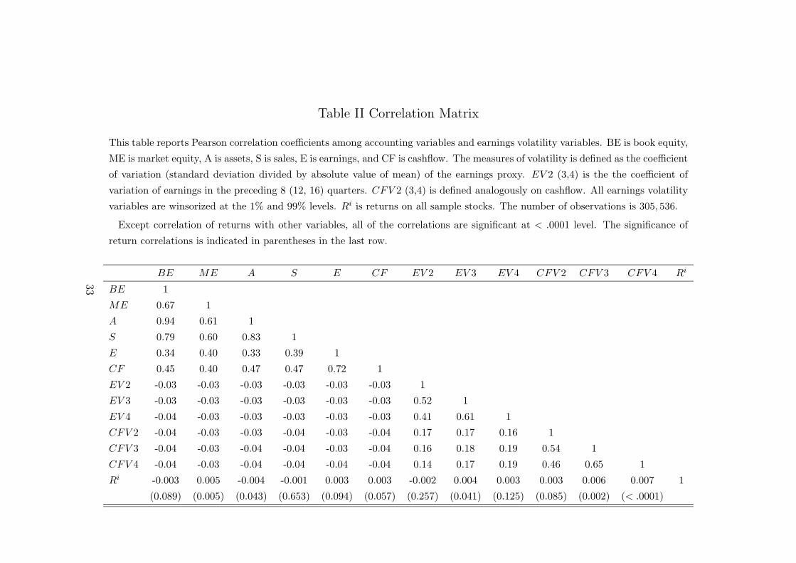
Table II Correlation Matrix

This table reports Pearson correlation coefficients among accounting variables and earnings volatility variables. BE is book equity,

ME is market equity, A is assets, S is sales, E is earnings, and CF is cashflow. The measures of volatility is defined as the coefficient

of variation (standard deviation divided by absolute value of mean) of the earnings proxy. EV 2 (3,4) is the the coefficient of

variation of earnings in the preceding 8 (12, 16) quarters. CFV 2 (3,4) is defined analogously on cashflow. All earnings volatility

variables are winsorized at the 1% and 99% levels. Ri is returns on all sample stocks. The number of observations is 305, 536.

Except correlation of returns with other variables, all of the correlations are significant at < .0001 level. The significance of

return correlations is indicated in parentheses in the last row.

BE ME A S E CF EV 2 EV 3 EV 4 CFV 2 CFV 3 CFV 4 Ri

BE 1

ME 0.67 1

A 0.94 0.61 1

S 0.79 0.60 0.83 1

E 0.34 0.40 0.33 0.39 1

CF 0.45 0.40 0.47 0.47 0.72 1

EV 2 -0.03 -0.03 -0.03 -0.03 -0.03 -0.03 1

EV 3 -0.03 -0.03 -0.03 -0.03 -0.03 -0.03 0.52 1

EV 4 -0.04 -0.03 -0.03 -0.03 -0.03 -0.03 0.41 0.61 1

CFV 2 -0.04 -0.03 -0.03 -0.04 -0.03 -0.04 0.17 0.17 0.16 1

CFV 3 -0.04 -0.03 -0.04 -0.04 -0.03 -0.04 0.16 0.18 0.19 0.54 1

CFV 4 -0.04 -0.03 -0.04 -0.04 -0.04 -0.04 0.14 0.17 0.19 0.46 0.65 1

Ri -0.003 0.005 -0.004 -0.001 0.003 0.003 -0.002 0.004 0.003 0.003 0.006 0.007 1

(0.089) (0.005) (0.043) (0.653) (0.094) (0.057) (0.257) (0.041) (0.125) (0.085) (0.002) (< .0001)

33

Table III Properties of Portfolios Formed on Book Equity: January 1971 to

December 2002

Each month 10 portfolios are formed on ranked values of book equity of latest fiscal quarter. Each decile portfolio

return is the weighted average return of all firm returns of that decile, weighted by market equity. Market equity

(ME), book equity (BE), sales (S), operating earnings (E) and cashflow (CF ) are simple aggregate of those

variables of all of the firms in a decile portfolio. EY is the earnings yield, defined as portfolio earnings (E) divided

by lagged one market equity, and BE/ME is defined as portfolio book equity divided by lagged one market equity.

EV 2, EV 3 and EV 4 (CFV 2, CFV 3 and CFV 4) are the coefficient of variation of all earnings (cashflows) of the

decile firms traced by an estimation window of 2, 3 and 4 years respectively. All earnings volatility variables are

winsorized at the 1% and 99% levels for the overall sample.

Portfolio 1 2 3 4 5 6 7 8 9 10

Return 3.64% 4.00% 3.65% 3.48% 3.09% 2.95% 2.54% 2.19% 1.89% 1.44%

ln(ME) 9.17 8.56 8.99 9.44 9.88 10.37 10.86 11.41 12.25 14.03

ln(BE) 6.17 7.51 8.18 8.73 9.22 9.69 10.20 10.78 11.60 13.49

ln(S) 8.75 7.55 8.15 8.65 9.01 9.49 9.93 10.44 11.23 13.01

E -1,674.30 -219.64 -216.68 -176.57 -144.08 45.36 433.75 1,350.28 4,149.55 41,245.20

CF -875.11 -128.32 -45.13 114.15 261.84 686.83 1,485.81 3,579.06 8,763.98 65,489.62

BE/ME -0.04 0.46 0.52 0.55 0.57 0.55 0.56 0.57 0.56 0.63

EY -0.04 -0.01 0.00 0.00 0.01 0.01 0.01 0.02 0.02 0.02

EV 2 13.94 7.98 7.35 15.05 22.71 14.52 6.89 4.64 2.75 2.48

EV 3 15.08 8.05 8.35 15.71 26.23 14.34 6.37 4.21 2.41 2.37

EV 4 14.96 8.19 9.76 18.03 30.52 12.84 5.60 3.55 2.23 2.34

CFV 2 5.12 2.27 3.58 2.07 1.10 0.99 0.62 0.59 0.58 0.67

CFV 3 5.66 3.38 4.28 2.00 1.37 0.90 0.65 0.62 0.60 0.70

CFV 4 5.49 3.41 5.17 1.77 1.13 0.90 0.69 0.66 0.63 0.72

Firms 433 432 432 432 432 433 433 432 433 432

34

Table IV Benchmark Regressions on Size-sorted Portfolios

This table presents panel regression results from the following two models:

Model 1: Rit = α + βmRm

t + βevEV 3it + εi

t,

Model 2: Rit = α + βmRm

t + βevCFV 3it + εi

t.

The dependent variable, Rit, is monthly returns, expressed in percent, on 10 size portfolios

sorted on book equity from January 1971 to December 2002 for model 1, and from January 1975

to December 2002 for model 2. Rm is the market return expressed in percent, and EV 3 (CFV 3) is

the earnings (cashflow) volatility of the portfolio estimated with the preceding 12 quarters’ earnings

(cashflow). White-consistent estimators are heteroscedasticity-consistent covariance matrix estima-

tors as in White (1980). Newey-West estimators are autocorrelation-corrected estimators with a

lag of 2 as in Newey and West (1987).

∗, ∗∗, and ∗∗∗ indicate significant at 1%, 5% and 10% respectively. In cases with no significance,

the associated p-values are indicated in parentheses below the parameter estimates.

Dependent variable: Size-sorted decile portfolio return

Model 1 Model 2

White- Newey- White- Newey-

OLS Consistent West GMM OLS Consistent West GMM

Intercept 1.482∗ 1.482∗ 1.482∗ 1.482∗ 1.653∗ 1.653∗ 1.653∗ 1.653∗

Rm 1.2854∗ 1.2854∗ 1.2854∗ 1.2854∗ 1.2926∗ 1.2926∗ 1.2926∗ 1.2926∗

EV 3 0.0218∗ 0.0218∗ 0.0218∗ 0.0218∗

CFV 3 0.0065∗ 0.0065∗ 0.0065∗ 0.0065∗

N 3,762 3,762 3,762 3,762 3,292 3,292 3,292 3,292

R2 0.592 0.592 0.592 0.592 0.565 0.565 0.565 0.565

35

Table V Regressions with Measures of Earnings Volatility of Different

Estimation Windows

This table presents results from panel regressions of the form

Ri

t= α + βmRm

t+ βevEV i

t+ εi

t

with these earnings volatility measures for EV : EV 2 ,EV 4 , CFV 2, and CFV 4. EV 2 (4) is earnings

volatility of the portfolio estimated with the preceding 8 (16) quarters’ earnings. CFV 2 (4) is defined

analogously with cashflow. The dependent variable, Ri

t, is monthly returns, expressed in percent, on 10

book equity-sorted portfolios from January 1971 to December 2002 for regressions with EV 2 and EV 4, and

from January 1975 to December 2002 for regressions with CFV 2 and CFV 4. Rm is the market return

expressed in percent. Panel A reports OLS regression results, and Panel B reports GMM regression results.

∗, ∗∗, and ∗∗∗ indicate significant at 1%, 5% and 10% respectively. In cases with no significance, the

associated p-values are indicated in parentheses below the parameter estimates.

Dependent variable: Size sorted decile portfolio return

Panel A: OLS

Intercept Rm EV 2 EV 4 CFV 2 CFV 4 R2

1.536∗ 1.283∗ 0.0162∗ 0.587

1.541∗ 1.280∗ 0.0151∗ 0.590

1.680∗ 1.288∗ 0.0052∗ 0.567

1.580∗ 1.285∗ 0.0117∗ 0.567

Panel B: GMM

Intercept Rm EV 2 EV 4 CFV 2 CFV 4 R2

1.536∗ 1.283∗ 0.0162∗ 0.587

1.541∗ 1.280∗ 0.0151∗ 0.590

1.680∗ 1.288∗ 0.0052∗ 0.567

1.580∗ 1.285∗ 0.0117∗ 0.567

36

Table VI Regressions with Traditional Return-informative Variables

This table presents results from panel regressions of size-sorted portfolio returns on earnings volatility

and different sets of traditional return-informative variables. The dependent variable, Ri

t, is monthly returns,

expressed in percent, on 10 book equity-sorted portfolios from January 1971 to December 2002 for regressions

with EV 3, which is earnings volatility of the portfolio estimated with the preceding 12 quarters’ earnings

(cashflow), and from January 1975 to December 2002 for regressions with CFV 3, which is earnings volatility

of the portfolio estimated with the preceding 12 quarters’ cashflows. EY is the portfolio earnings yield,

defined as last quarter’s earnings divided by lagged one market equity. BM is the portfolio book-to-market

equity, defined as book equity divided by lagged one market equity. ln(ME) is the logarithm of lagged

one market equity. RV is the portfolio’s return volatility, defined as the standard deviation of returns on

the same decile portfolio over the past 36 months. Panels A1 and A2 report respectively OLS and GMM

regression results for EV 3, and Panels B1 and B2 are for CFV 3.

∗, ∗∗, and ∗∗∗ indicate significant at 1%, 5% and 10% respectively. In cases with no significance, the

associated p-values are indicated in parentheses below the parameter estimates.

Dependent variable: Size-sorted decile portfolio returns

Panel A1: EV3 as earnings volatility, OLS regressions

Intercept Rm EV 3 EY BM ln(ME) RV R2

1.671∗ 1.281∗ 0.0128∗ −0.281∗ 0.6024

1.122∗ 1.278∗ 0.0147∗ −0.364∗ 1.134∗ 0.6041

0.287 1.278∗ 0.0155∗ −0.384∗ 1.342∗ 0.070∗∗∗ 0.6044

(0.581)

−2.344∗ 1.297∗ 0.0092∗∗ −0.237∗ 0.740∗∗ 0.133∗ 32.168∗ 0.6142

Panel A2: EV3 as earnings volatility, GMM regressions

1.667∗ 1.281∗ 0.0126 −0.281∗ 0.6024

(0.123)

1.122∗ 1.278∗ 0.0145∗∗∗ −0.364∗ 1.126∗∗ 0.6041

0.230 1.278∗ 0.0153∗∗ −0.385∗ 1.349∗∗ 0.074 0.6044

(0.739) (0.164)

−2.344∗∗ 1.297∗ 0.0092 −0.237∗ 0.740 0.133∗∗ 32.168∗ 0.6142

(0.236)

37

Dependent variable: Size-sorted decile portfolio returns

Panel B1: CFV3 as earnings volatility, OLS regressions

Intercept Rm CFV 3 EY BM ln(ME) RV R2

1.757∗ 1.293∗ 0.0031∗∗∗ −0.241∗ 0.5737

1.231∗ 1.289∗ 0.0044∗ −0.306∗ 1.107∗ 0.5750

1.668∗ 1.288∗ 0.0040∗∗ −0.297∗ 0.993 −0.357 0.5750

(0.466)

−1.423∗∗ 1.313∗ 0.0031∗∗∗ −0.190∗ 0.270 −0.081 29.106∗ 0.5850

(0.487) (0.107)

Panel B2: CFV3 as earnings volatility, GMM regressions

1.757∗ 1.293∗ 0.0031 −0.241∗ 0.5737

(0.152)

1.231∗ 1.289∗ 0.0044∗∗ −0.306∗ 1.107∗∗∗ 0.5750

1.668∗∗ 1.288∗ 0.0040∗∗∗ −0.297∗ 0.993∗∗∗ −0.357 0.5750

(0.551)

−1.423 1.313∗ 0.0031 −0.190∗ 0.270 −0.081 29.106∗ 0.5850

(0.221) (0.178) (0.669) (0.275)

38

Table VII Regressions with Traditional Return-informative Variables and

Other Earnings Volatility Measures

This table presents results from panel regressions of size-sorted portfolio returns on earnings volatility

and different sets of traditional return-informative variables. The dependent variable, Ri

t, is monthly returns,

expressed in percent, on 10 book equity-sorted portfolios from January 1971 to December 2002 for regressions

with EV 2 and EV 4, which are respectively earnings volatility of the portfolio estimated with the preceding 8

and 16 quarters’ earnings, and from January 1975 to December 2002 for regressions with CFV 2 and CFV 4,

which are respectively earnings volatility of the portfolio estimated with the preceding 8 and 16 quarters’

cashflow. EY is the portfolio earnings yield, defined as last quarter’s earnings divided by lagged one market

equity. BM is the portfolio book-to-market ratio, defined as book equity divided by lagged one market

equity. ln(ME) is the logarithm of lagged one market equity. RV is the portfolio’s return volatility, defined

as the standard deviation of returns on the same decile portfolio over the past 36 months. The regression

method is OLS.

∗, ∗∗, and ∗∗∗ indicate significant at 1%, 5% and 10% respectively. In cases with no significance, the

associated p-values are indicated in parentheses below the parameter estimates.

Dependent variable: Size-sorted decile portfolio returns

Panel A: Earnings volatility using EV 2 and EV 4

Intercept Rm EV 2 EV 4 EY BM ln(ME) RV

1.216∗ 1.276∗ 0.0085∗∗∗ −0.365∗ 1.060∗

0.433 1.276∗ 0.0091∗∗∗ −0.384∗ 1.255∗ 0.065

(0.406) (0.111)

−2.259∗ 1.295∗ 0.0026 −0.236∗ 0.657∗∗ 0.131∗ 32.691∗

(0.603)

1.217∗ 1.273∗ 0.0087∗∗ −0.363∗ 1.053∗

0.390 1.273∗ 0.0093∗∗ −0.383∗ 1.259∗ 0.069∗∗∗

(0.453)

−2.366∗ 1.292∗ 0.0043 −0.231∗ 0.649∗∗ 0.136∗ 33.344∗

(0.305)

39

Panel B: Earnings volatility using CFV 2 and CFV 4

Intercept Rm CFV 2 CFV 4 EY BM ln(ME) RV

1.349∗ 1.285∗ 0.0018 −0.303∗ 0.962∗

(0.381)

2.040∗ 1.284∗ 0.0011 −0.288∗ 0.777∗ −0.056

(0.591) (0.252)

−1.106 1.310∗ 0.0003 −0.181∗ 0.046 0.063 29.549∗

(0.123) (0.903) (0.907) (0.211)

1.092∗ 1.281∗ 0.0094∗ −0.293∗ 1.230∗

1.209∗∗∗ 1.281∗ 0.0093∗ −0.290∗ 1.199∗ −0.010

(0.845)

−1.761∗∗ 1.307∗ 0.0081∗ −0.186∗ 0.468 0.102∗∗ 28.438∗

(0.230)

40

Table VIII Time-series Regressions with Fama-French’s (1993) Three

Factors and a Earnings Volatility Mimicking Portfolio Factor

This table presents results from time-series regressions of the form

Rit − Rf

t = α + βim(Rm

t − Rft ) + βi

SMBSMBit + βi

HMLHMLit + βi

V MF V MF it + εi

t

for each cross-section i from Jan. 1972 to Dec. 2002. The regression method is OLS. Following

Fama and French (1993), 25 cross-sectional portfolios are formed by quintiles of size, proxied by

market equity, and quintiles of book-to-market equity ratio. Rit is the value-weighted portfolio

return. Rm is the monthly CRSP value weighted NYSE/NASDAQ/AMEX index return. Rf is

the monthly 90-day treasury bill return. SMB and HML are Fama-French’s (1993) size and value

mimicking portfolio returns respectively. V MF is returns on volatile-earnings stocks (V) minus

returns on flat-earnings stocks (F). Specifically, to construct SMB, HML and V MF , stocks in the

sample are divided into small (S) and big (B) based on the median stock size of the NYSE market

of June each year. Similarly, the sample stock are sorted on the book-to-market equity ratio of the

NYSE market in December of the preceding year, and then are divided into high (H) (the top 30%),

middle (M) (the middle 40%) and low (L)(the bottom 30%) book-to-market equity. In addition,

the sample stocks are divided into groups of volatile (V) and flat (F) earnings based on the median

earnings volatility (proxied by EV 3, or the absolute coefficient of variation of earnings estimated

with the prior 12 quarters’ earnings) of the NYSE market of December each year. SMB is the

simple average of returns on the three small-portfolios (S/L, S/M, S/H) minus the simple average

of returns on the three big-portfolios (B/L, B/M, B/H). HML is the simple average of returns on

two high book-to-market equity ratio portfolios (S/H, B/H) minus the simple average of returns on

two low book-to-market equity ratio portfolios (S/L, B/L). V MF is the simple average of returns

on the three volatile earnings portfolios (V/H, V/M, V/L) minus the simple average of returns on

the three flat earnings portfolios (F/H, F/M, F/L).

41

Dependent variable: Excess return on 25 stock portfolios formed on size and book-to-market equity

Book-to-market equity quintiles

Size quintile Low 2 3 4 High Low 2 3 4 High

Intercept P(Intercept)

Small 0.00 0.00 0.00 0.00 0.01 0.607 0.794 0.611 0.000 0.000

2 0.01 0.01 0.01 0.01 0.01 0.000 0.000 0.000 0.000 0.000

3 0.01 0.01 0.01 0.01 0.01 0.000 0.000 0.000 0.000 0.000

4 0.01 0.01 0.01 0.01 0.01 0.000 0.000 0.000 0.000 0.000

Big 0.01 0.01 0.00 0.00 0.01 0.000 0.000 0.000 0.002 0.000

βRmP (βRm

)

Small 1.11 0.99 0.96 0.89 1.02 0.000 0.000 0.000 0.000 0.000

2 1.12 1.04 0.99 0.96 1.13 0.000 0.000 0.000 0.000 0.000

3 1.13 0.99 0.95 1.01 1.13 0.000 0.000 0.000 0.000 0.000

4 1.07 1.01 0.95 1.05 1.09 0.000 0.000 0.000 0.000 0.000

Big 1.04 0.93 0.83 0.93 1.07 0.000 0.000 0.000 0.000 0.000

βSMB P (βSMB)

Small 1.01 0.84 0.78 0.75 0.83 0.000 0.000 0.000 0.000 0.000

2 0.83 0.57 0.51 0.50 0.56 0.000 0.000 0.000 0.000 0.000

3 0.52 0.41 0.34 0.32 0.37 0.000 0.000 0.000 0.000 0.000

4 0.24 0.17 0.12 0.08 0.17 0.000 0.000 0.000 0.027 0.000

Big -0.17 -0.12 -0.10 -0.07 -0.04 0.000 0.000 0.005 0.093 0.466

βHML P (βHML)

Small -0.21 -0.06 0.20 0.41 0.69 0.000 0.143 0.000 0.000 0.000

2 -0.50 -0.08 0.22 0.46 0.68 0.000 0.024 0.000 0.000 0.000

3 -0.58 0.02 0.26 0.60 0.60 0.000 0.600 0.000 0.000 0.000

4 -0.49 0.12 0.33 0.56 0.54 0.000 0.000 0.000 0.000 0.000

Big -0.37 0.11 0.22 0.49 0.68 0.000 0.000 0.000 0.000 0.000

βV MF P (βV MF )

Small 0.46 0.38 0.29 0.28 0.34 0.000 0.000 0.000 0.000 0.000

2 0.34 0.25 0.15 0.17 0.21 0.000 0.000 0.001 0.000 0.000

3 0.23 0.14 0.06 0.18 0.14 0.000 0.001 0.162 0.000 0.006

4 0.22 0.13 0.07 0.09 0.17 0.000 0.002 0.118 0.059 0.006

Big -0.04 0.07 0.09 0.05 0.30 0.213 0.071 0.047 0.303 0.000

R2

Small 0.85 0.86 0.86 0.87 0.86

2 0.88 0.87 0.84 0.83 0.85

3 0.87 0.83 0.81 0.84 0.80

4 0.88 0.83 0.79 0.79 0.70

Big 0.91 0.80 0.71 0.70 0.6342

Table IX Regressions with Portfolios Sorted on Other Measures of Size

This table presents results from regressions of the form

Rit = α + βmRm

t + βevEV it + εi

t,

The dependent variable, Rit, is monthly returns, expressed in percent, on 10 size portfolios

sorted on these size measures: lagged market equity (lagged ME), total assets, and sales. The

sample period is from January 1971 to December 2002 for regressions with EV 3, and from January

1975 to December 2002 for regressions with CFV 3. EV 3 or CFV 3 (the absolute coefficient of

variation of earnings estimated with the prior 12 quarters’ earnings or cashflow) is used to proxy

for earnings volatility (EV ). Rm is the market return expressed in percent. The regression method

is GMM.

∗, ∗∗, and ∗∗∗ indicate significant at 1%, 5% and 10% respectively. In cases with no significance,

the associated p-values are indicated in parentheses below the parameter estimates.

Dependent variable: Size-sorted portfolio return

Portfolios sorted on Intercept Rm EV 3 CFV 3 R2

Lagged ME 2.225∗ 1.185∗ 0.012∗ 0.462

2.445∗ 1.184∗ 0.0115∗ 0.470

Total Assets 1.701∗ 1.309∗ 0.0041 0.536

(0.384)

1.591∗ 1.326∗ 0.035∗ 0.515

Sales 1.297∗ 1.305∗ 0.0078 0.570

(0.135)

1.302∗ 1.333∗ 0.0143∗∗ 0.533

43

Table X Robustness: Sub-sample and sub-periods

This table presents results from regressions of the form

Rit = α + βmRm

t + βevEV it + εi

t

using the sub-sample of NYSE stocks from January 1971 to December 2002 only, and two ten-year

sub-periods of 1976-1985 and 1986-1995 with all stocks listed in NYSE, NASDAQ, and AMEX. Rit

are the value-weighted returns (in percent) on 10-decile portfolios sorted on book equity. Rm is the

monthly CRSP value weighted NYSE/NASDAQ/AMEX index return (in percent). EV 3 or CFV 3

(the absolute coefficient of variation of earnings estimated with the prior 12 quarters’ earnings or

cashflow) is used to proxy for earnings volatility (EV ). The regression method is GMM.

∗, ∗∗, and ∗∗∗ indicate significant at 1%, 5% and 10% respectively. In cases with no significance,

the associated p-values are indicated in parentheses below the parameter estimates.

Dependent variable: Book equity-sorted portfolio return

Intercept Rm EV 3 CFV 3 R2

NYSE Subsample 0.876∗ 1.022∗ 0.008∗∗∗ 0.462

0.862∗ 1.011∗ 0.0315∗ 0.729

Sub-period: 1976-1985 1.147∗ 1.326∗ 0.0127 0.713

(0.320)

1.0098∗ 1.317∗ 0.0152∗∗ 0.706

Sub-period: 1986-1995 1.457∗ 1.180∗ 0.0032 0.665

(0.301)

1.302∗ 1.173∗ 0.0027∗∗ 0.658

44

Table XI Average Slopes (t-Statistics) from Fama-French (1992) Month-to-Month Regressions

of Stock Returns on β, Size, Book-to-Market Equity, and Earnings Volatility: January 1975 to

December 2002

This table presents monthly averages from the Fama and French (1992) type cross-sectional regressions

of monthly returns of all NYSE/NASDAQ/AMEX listed firm on β, size, book-to-market equity and earnings

volatility measures from Jan. 1975 to Dec. 2002. Fama-MacBeth (1973) procedure is used to estimate the full

period βs of 100 size-β sorted portfolios, and then stocks are assigned the full-period β of the portfolio they

are in at the end of each June. Firm size ln(ME) is market equity measured in latest June. Book-to-market

equity (BE/ME) is measured by book equity of latest fiscal year divided by market equity of December of

the same year. EV 3 (EV 4) is the absolute coefficient of variation of earnings estimated with the prior 12

(16) quarters’ earnings. CFV 3 (CFV 4) is the absolute coefficient of variation of cashflow estimated with

the prior 12 (16) quarters’ cashflow.

The estimates are the averages of the time-series coefficients of the monthly regression slopes for Jan.

1975 to Dec. 2002, and the t-statistics are the average slopes divided by their time-series standard error.

β ln(ME) ln(BE/ME) EV 3 EV 4 CFV 3 CFV 4

0.04 -0.20 0.25

(0.13) (-2.47) (2.98)

0.21

(0.97)

0.21

(1.00)

-0.14

(-0.89)

-0.14

(-0.90)

0.28 0.21

(0.76) (0.98)

0.27 0.21

(0.74) (1.00)

0.21 -0.14

(0.57) (-0.83)

0.22 -0.14

(0.59) (-0.84)

0.01 -0.18 0.22 0.16

(0.03) (-2.75) (2.33) (0.86)

0.01 -0.18 0.22 0.16

(0.02) (-2.72) (2.32) (0.89)

0.04 -0.21 0.25 -0.03

(0.12) (-2.54) (2.94) (-0.37)

0.04 -0.21 0.25 -0.03

(0.13) (-2.55) (2.95) (-0.37)

45