the cotton tensor and the ricci flow - cvgmt: homecvgmt.sns.it/media/doc/paper/1809/cotton.pdf ·...
TRANSCRIPT

THE COTTON TENSOR AND THE RICCI FLOW
CARLO MANTEGAZZA, SAMUELE MONGODI, AND MICHELE RIMOLDI
ABSTRACT. We compute the evolution equation of the Cotton and the Bach tensor under the Ricci flowof a Riemannian manifold, with particular attention to the three dimensional case, and we discuss someapplications.
CONTENTS
1. Preliminaries 12. The Evolution Equation of the Cotton Tensor in 3D 23. Three–Dimensional Gradient Ricci Solitons 104. The Evolution Equation of the Cotton Tensor in any Dimension 135. The Bach Tensor 235.1. The Evolution Equation of the Bach Tensor in 3D 245.2. The Bach Tensor of Three–Dimensional Gradient Ricci Solitons 26References 28
1. PRELIMINARIES
The Riemann curvature operator of a Riemannian manifold (Mn, g) is defined, as in [6], by
Riem(X,Y )Z = ∇Y∇XZ −∇X∇Y Z +∇[X,Y ]Z .
In a local coordinate system the components of the (3, 1)–Riemann curvature tensor are given byRl
ijk∂∂xl = Riem
(∂∂xi ,
∂∂xj
)∂
∂xk and we denote by Rijkl = glmRmijk its (4, 0)–version.
With the previous choice, for the sphere Sn we have Riem(v, w, v, w) = Rabcdviwjvkwl > 0.
In all the paper the Einstein convention of summing over the repeated indices will be adopted.
The Ricci tensor is obtained by the contraction Rik = gjlRijkl and R = gikRik will denote the scalarcurvature.
We recall the interchange of derivative formula,
∇2ijωk −∇2
jiωk = Rijkpgpqωq ,
and Schur lemma, which follows by the second Bianchi identity,
2gpq∇pRqi = ∇iR .
They both will be used extensively in the computations that follows.
The so called Weyl tensor is then defined by the following decomposition formula (see [6, Chapter 3,Section K]) in dimension n ≥ 3,
(1.1) Rijkl =1
n− 2(Rikgjl − Rilgjk + Rjlgik − Rjkgil)−
R
(n− 1)(n− 2)(gikgjl − gilgjk) + Wijkl .
The Weyl tensor satisfies all the symmetries of the curvature tensor, moreover, all its traces with themetric are zero, as it can be easily seen by the above formula.In dimension three W is identically zero for every Riemannian manifold. It becomes relevant insteadwhen n ≥ 4 since its vanishing is a condition equivalent for (Mn, g) to be locally conformally flat, that is,around every point p ∈Mn there is a conformal deformation gij = efgij of the original metric g, suchthat the new metric is flat, namely, the Riemann tensor associated to g is zero in Up (here f : Up → Ris a smooth function defined in a open neighborhood Up of p).
Date: March 4, 2014.1
2 CARLO MANTEGAZZA, SAMUELE MONGODI, AND MICHELE RIMOLDI
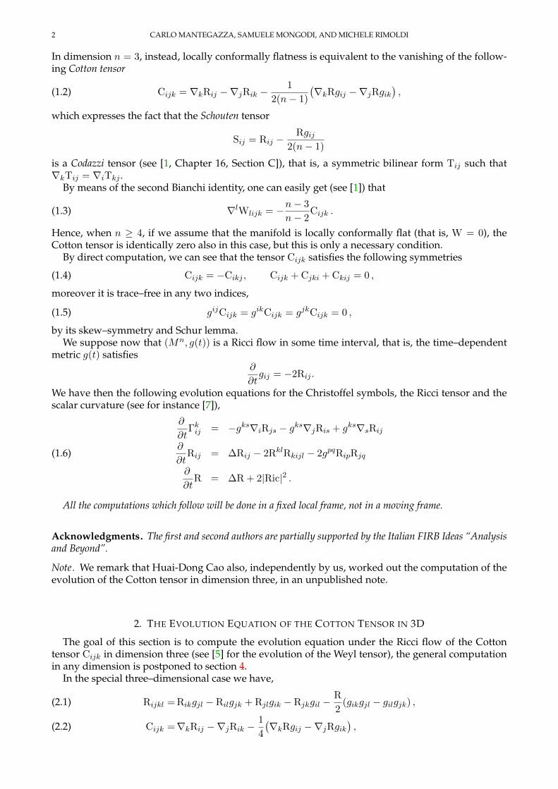
In dimension n = 3, instead, locally conformally flatness is equivalent to the vanishing of the follow-ing Cotton tensor
(1.2) Cijk = ∇kRij −∇jRik −1
2(n− 1)
(∇kRgij −∇jRgik
),
which expresses the fact that the Schouten tensor
Sij = Rij −Rgij
2(n− 1)
is a Codazzi tensor (see [1, Chapter 16, Section C]), that is, a symmetric bilinear form Tij such that∇kTij = ∇iTkj .
By means of the second Bianchi identity, one can easily get (see [1]) that
(1.3) ∇lWlijk = −n− 3
n− 2Cijk .
Hence, when n ≥ 4, if we assume that the manifold is locally conformally flat (that is, W = 0), theCotton tensor is identically zero also in this case, but this is only a necessary condition.
By direct computation, we can see that the tensor Cijk satisfies the following symmetries
(1.4) Cijk = −Cikj , Cijk + Cjki + Ckij = 0 ,
moreover it is trace–free in any two indices,
(1.5) gijCijk = gikCijk = gjkCijk = 0 ,
by its skew–symmetry and Schur lemma.We suppose now that (Mn, g(t)) is a Ricci flow in some time interval, that is, the time–dependent
metric g(t) satisfies∂
∂tgij = −2Rij .
We have then the following evolution equations for the Christoffel symbols, the Ricci tensor and thescalar curvature (see for instance [7]),
∂
∂tΓkij = −gks∇iRjs − gks∇jRis + gks∇sRij
∂
∂tRij = ∆Rij − 2RklRkijl − 2gpqRipRjq(1.6)
∂
∂tR = ∆R + 2|Ric|2 .
All the computations which follow will be done in a fixed local frame, not in a moving frame.
Acknowledgments. The first and second authors are partially supported by the Italian FIRB Ideas “Analysisand Beyond”.
Note. We remark that Huai-Dong Cao also, independently by us, worked out the computation of theevolution of the Cotton tensor in dimension three, in an unpublished note.
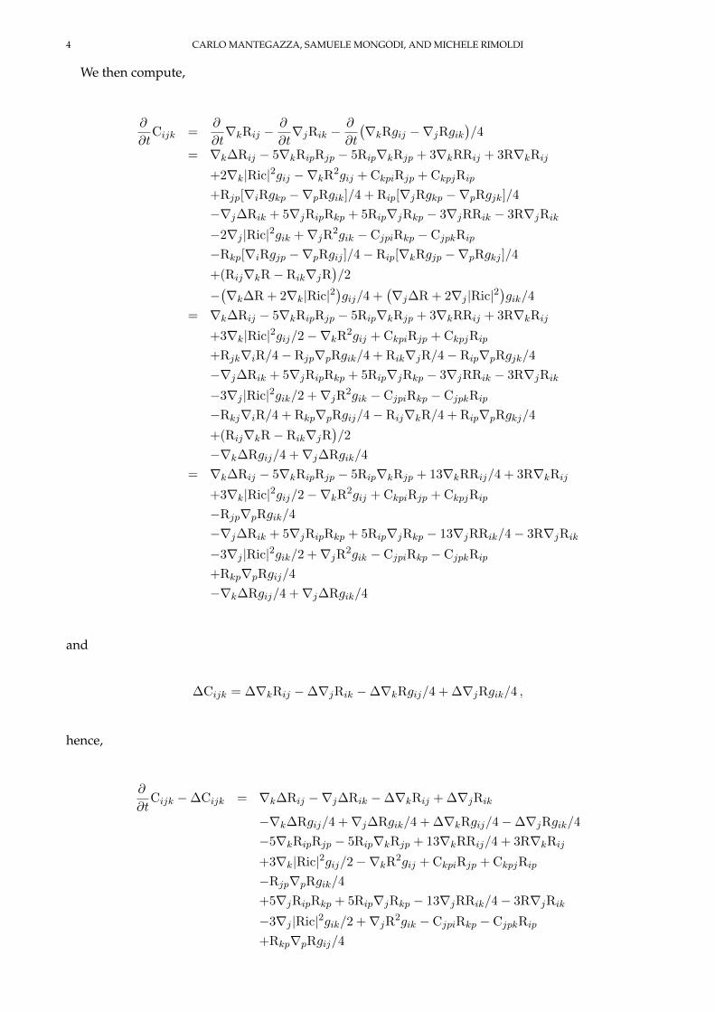
2. THE EVOLUTION EQUATION OF THE COTTON TENSOR IN 3D
The goal of this section is to compute the evolution equation under the Ricci flow of the Cottontensor Cijk in dimension three (see [5] for the evolution of the Weyl tensor), the general computationin any dimension is postponed to section 4.
In the special three–dimensional case we have,
Rijkl = Rikgjl − Rilgjk + Rjlgik − Rjkgil −R
2(gikgjl − gilgjk) ,(2.1)
Cijk =∇kRij −∇jRik −1
4
(∇kRgij −∇jRgik
),(2.2)

THE COTTON TENSOR AND THE RICCI FLOW 3
hence, the evolution equations (1.6) become
∂
∂tΓkij = − gks∇iRjs − gks∇jRis + gks∇sRij
∂
∂tRij = ∆Rij − 6gpqRipRjq + 3RRij + 2|Ric|2gij − R2gij
∂
∂tR = ∆R + 2|Ric|2 .
From these formulas we can compute the evolution equations of the derivatives of the curvaturesassuming, from now on, to be in normal coordinates,
∂
∂t∇lR = ∇l∆R + 2∇l|Ric|2 ,
∂
∂t∇sRij = ∇s∆Rij − 6∇sRipRjp − 6Rip∇sRjp + 3∇sRRij + 3R∇sRij
+2∇s|Ric|2gij −∇sR2gij
+(∇iRsp +∇sRip −∇pRis)Rjp
+(∇jRsp +∇sRjp −∇pRjs)Rip
= ∇s∆Rij − 5∇sRipRjp − 5Rip∇sRjp + 3∇sRRij + 3R∇sRij
+2∇s|Ric|2gij −∇sR2gij
+(∇iRsp −∇pRis)Rjp + (∇jRsp −∇pRjs)Rip
= ∇s∆Rij − 5∇sRipRjp − 5Rip∇sRjp + 3∇sRRij + 3R∇sRij
+2∇s|Ric|2gij −∇sR2gij + CspiRjp + CspjRip
+Rjp[∇iRgsp −∇pRgis]/4 + Rip[∇jRgsp −∇pRgjs]/4 ,
where in the last passage we substituted the expression of the Cotton tensor.
4 CARLO MANTEGAZZA, SAMUELE MONGODI, AND MICHELE RIMOLDI
We then compute,
∂
∂tCijk =
∂
∂t∇kRij −
∂
∂t∇jRik −
∂
∂t
(∇kRgij −∇jRgik
)/4
= ∇k∆Rij − 5∇kRipRjp − 5Rip∇kRjp + 3∇kRRij + 3R∇kRij
+2∇k|Ric|2gij −∇kR2gij + CkpiRjp + CkpjRip
+Rjp[∇iRgkp −∇pRgik]/4 + Rip[∇jRgkp −∇pRgjk]/4
−∇j∆Rik + 5∇jRipRkp + 5Rip∇jRkp − 3∇jRRik − 3R∇jRik
−2∇j |Ric|2gik +∇jR2gik − CjpiRkp − CjpkRip
−Rkp[∇iRgjp −∇pRgij ]/4− Rip[∇kRgjp −∇pRgkj ]/4
+(Rij∇kR− Rik∇jR)/2
−(∇k∆R + 2∇k|Ric|2
)gij/4 +
(∇j∆R + 2∇j |Ric|2
)gik/4
= ∇k∆Rij − 5∇kRipRjp − 5Rip∇kRjp + 3∇kRRij + 3R∇kRij
+3∇k|Ric|2gij/2−∇kR2gij + CkpiRjp + CkpjRip
+Rjk∇iR/4− Rjp∇pRgik/4 + Rik∇jR/4− Rip∇pRgjk/4
−∇j∆Rik + 5∇jRipRkp + 5Rip∇jRkp − 3∇jRRik − 3R∇jRik
−3∇j |Ric|2gik/2 +∇jR2gik − CjpiRkp − CjpkRip
−Rkj∇iR/4 + Rkp∇pRgij/4− Rij∇kR/4 + Rip∇pRgkj/4
+(Rij∇kR− Rik∇jR)/2
−∇k∆Rgij/4 +∇j∆Rgik/4
= ∇k∆Rij − 5∇kRipRjp − 5Rip∇kRjp + 13∇kRRij/4 + 3R∇kRij
+3∇k|Ric|2gij/2−∇kR2gij + CkpiRjp + CkpjRip
−Rjp∇pRgik/4
−∇j∆Rik + 5∇jRipRkp + 5Rip∇jRkp − 13∇jRRik/4− 3R∇jRik
−3∇j |Ric|2gik/2 +∇jR2gik − CjpiRkp − CjpkRip
+Rkp∇pRgij/4
−∇k∆Rgij/4 +∇j∆Rgik/4
and
∆Cijk = ∆∇kRij −∆∇jRik −∆∇kRgij/4 + ∆∇jRgik/4 ,
hence,
∂
∂tCijk −∆Cijk = ∇k∆Rij −∇j∆Rik −∆∇kRij + ∆∇jRik
−∇k∆Rgij/4 +∇j∆Rgik/4 + ∆∇kRgij/4−∆∇jRgik/4
−5∇kRipRjp − 5Rip∇kRjp + 13∇kRRij/4 + 3R∇kRij
+3∇k|Ric|2gij/2−∇kR2gij + CkpiRjp + CkpjRip
−Rjp∇pRgik/4
+5∇jRipRkp + 5Rip∇jRkp − 13∇jRRik/4− 3R∇jRik
−3∇j |Ric|2gik/2 +∇jR2gik − CjpiRkp − CjpkRip
+Rkp∇pRgij/4

THE COTTON TENSOR AND THE RICCI FLOW 5
Now to proceed, we need the following commutation rules for the derivatives of the Ricci tensorand of the scalar curvature, where we will employ the special form of the Riemann tensor in dimen-sion three given by formula (2.1),
∇k∆Rij −∆∇kRij = ∇3kllRij −∇3
lklRij +∇3lklRij −∇3
llkRij
= −Rkp∇pRij + Rklip∇lRjp + Rkljp∇lRip
+∇3lklRij −∇3
llkRij
= −Rkp∇pRij + Rik∇jR/2 + Rjk∇iR/2
−Rkp∇iRjp − Rkp∇jRip + Rlp∇lRjpgik + Rlp∇lRipgjk
−Rli∇lRjk − Rlj∇lRik − R∇jRgik/4− R∇iRgjk/4
+R∇iRjk/2 + R∇jRik/2
+∇l
(RklipRpj + RkljpRpi
)= −Rkp∇pRij + Rik∇jR/2 + Rjk∇iR/2
−Rkp∇iRjp − Rkp∇jRip + Rlp∇lRjpgik + Rlp∇lRipgjk
−Rli∇lRjk − Rlj∇lRik − R∇jRgik/4− R∇iRgjk/4
+R∇iRjk/2 + R∇jRik/2
+∇l
(RikRlj − RilRkj + RplRpjgik − RpkRpjgil − gikRRlj/2 + gilRRjk/2
+RjkRli − RjlRki + RplRpigjk − RpkRpigjl − gjkRRli/2 + gjlRRik/2)
= −Rkp∇pRij + Rik∇jR/2 + Rjk∇iR/2
−Rkp∇iRjp − Rkp∇jRip + Rlp∇lRjpgik + Rlp∇lRipgjk
−Rli∇lRjk − Rlj∇lRik − R∇jRgik/4− R∇iRgjk/4
+R∇iRjk/2 + R∇jRik/2
−∇iRpkRpj +∇iRRjk/2 + gikRpl∇lRpj
−Rpk∇iRpj − gikR∇jR/4 + R∇iRjk/2
−∇jRpkRpi +∇jRRik/2 + gjkRpl∇lRpi
−Rpk∇jRpi − gjkR∇iR/4 + R∇jRik/2
= −Rkp∇pRij + Rik∇jR + Rjk∇iR
−2Rkp∇iRjp − 2Rkp∇jRip + 2Rlp∇lRjpgik + 2Rlp∇lRipgjk
−Rli∇lRjk − Rlj∇lRik − Rpj∇iRpk − Rpi∇jRpk
−R∇jRgik/2− R∇iRgjk/2 + R∇iRjk + R∇jRik
and
∇k∆R−∆∇kR = Rkllp∇pR = −Rkp∇pR .
6 CARLO MANTEGAZZA, SAMUELE MONGODI, AND MICHELE RIMOLDI
Then, getting back to the main computation, we obtain
∂
∂tCijk −∆Cijk = −Rkp∇pRij + Rik∇jR + Rjk∇iR
−2Rkp∇iRjp − 2Rkp∇jRip + 2Rlp∇lRjpgik + 2Rlp∇lRipgjk
−Rli∇lRjk − Rlj∇lRik − Rpj∇iRpk − Rpi∇jRpk
−R∇jRgik/2− R∇iRgjk/2 + R∇iRjk + R∇jRik
+Rjp∇pRik − Rij∇kR− Rkj∇iR
+2Rjp∇iRkp + 2Rjp∇kRip − 2Rlp∇lRkpgij − 2Rlp∇lRipgkj
+Rli∇lRkj + Rlk∇lRij + Rpk∇iRpj + Rpi∇kRpj
+R∇kRgij/2 + R∇iRgkj/2− R∇iRkj − R∇kRij
+Rkp∇pRgij/4− Rjp∇pRgik/4
−5∇kRipRjp − 5Rip∇kRjp + 13∇kRRij/4 + 3R∇kRij
+3∇k|Ric|2gij/2−∇kR2gij + CkpiRjp + CkpjRip
−Rjp∇pRgik/4
+5∇jRipRkp + 5Rip∇jRkp − 13∇jRRik/4− 3R∇jRik
−3∇j |Ric|2gik/2 +∇jR2gik − CjpiRkp − CjpkRip
+Rkp∇pRgij/4
= CkpiRjp + CkpjRip − CjpiRkp − CjpkRip
+[2Rlp∇lRjp + 3R∇jR/2− Rjp∇pR/2− 3∇j |Ric|2/2]gik
+[−2Rlp∇lRkp − 3R∇kR/2 + Rkp∇pR/2 + 3∇k|Ric|2/2]gij
−Rkp∇iRjp + Rjp∇iRkp
−3∇kRipRjp − 4Rip∇kRjp + 9∇kRRij/4 + 2R∇kRij
+3∇jRipRkp + 4Rip∇jRkp − 9∇jRRik/4− 2R∇jRik
Now, by means of the very definition of the Cotton tensor in dimension three (2.2) and the identi-ties (1.4), we substitute
Ckpj − Cjpk = − Ckjp − Cjpk = Cpkj
∇lRjp =∇jRlp + Cpjl +1
4
(∇lRgpj −∇jRgpl
)∇lRkp =∇kRlp + Cpkl +
1
4
(∇lRgpk −∇kRgpl
)∇iRjp =∇jRip + Cpji +
1
4
(∇iRgjp −∇jRgip
)∇iRkp =∇kRip + Cpki +
1
4
(∇iRgkp −∇kRgip
)
THE COTTON TENSOR AND THE RICCI FLOW 7
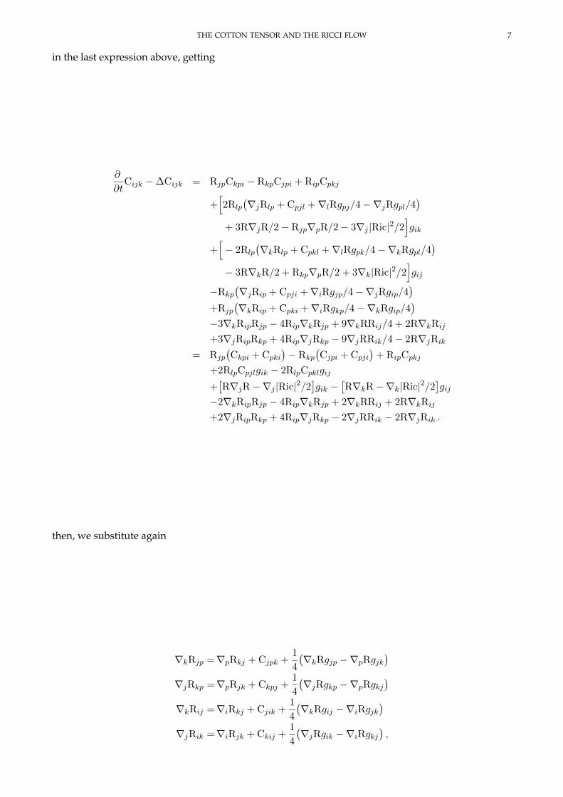
in the last expression above, getting
∂
∂tCijk −∆Cijk = RjpCkpi − RkpCjpi + RipCpkj
+[2Rlp
(∇jRlp + Cpjl +∇lRgpj/4−∇jRgpl/4
)+ 3R∇jR/2− Rjp∇pR/2− 3∇j |Ric|2/2
]gik
+[− 2Rlp
(∇kRlp + Cpkl +∇lRgpk/4−∇kRgpl/4
)− 3R∇kR/2 + Rkp∇pR/2 + 3∇k|Ric|2/2
]gij
−Rkp
(∇jRip + Cpji +∇iRgjp/4−∇jRgip/4
)+Rjp
(∇kRip + Cpki +∇iRgkp/4−∇kRgip/4
)−3∇kRipRjp − 4Rip∇kRjp + 9∇kRRij/4 + 2R∇kRij
+3∇jRipRkp + 4Rip∇jRkp − 9∇jRRik/4− 2R∇jRik
= Rjp
(Ckpi + Cpki
)− Rkp
(Cjpi + Cpji
)+ RipCpkj
+2RlpCpjlgik − 2RlpCpklgij
+[R∇jR−∇j |Ric|2/2
]gik −
[R∇kR−∇k|Ric|2/2
]gij
−2∇kRipRjp − 4Rip∇kRjp + 2∇kRRij + 2R∇kRij
+2∇jRipRkp + 4Rip∇jRkp − 2∇jRRik − 2R∇jRik .
then, we substitute again
∇kRjp =∇pRkj + Cjpk +1
4
(∇kRgjp −∇pRgjk
)∇jRkp =∇pRjk + Ckpj +
1
4
(∇jRgkp −∇pRgkj
)∇kRij =∇iRkj + Cjik +
1
4
(∇kRgij −∇iRgjk
)∇jRik =∇iRjk + Ckij +
1
4
(∇jRgik −∇iRgkj
),

8 CARLO MANTEGAZZA, SAMUELE MONGODI, AND MICHELE RIMOLDI
finally obtaining
∂
∂tCijk −∆Cijk = Rjp
(Ckpi + Cpki
)− Rkp
(Cjpi + Cpji
)+ RipCpkj
+2RlpCpjlgik − 2RlpCpklgij
+[R∇jR−∇j |Ric|2/2
]gik −
[R∇kR−∇k|Ric|2/2
]gij
−2∇kRipRjp − 4Rip
(∇pRkj + Cjpk +∇kRgjp/4−∇pRgjk/4
)+2∇kRRij + 2R
(∇iRkj + Cjik +∇kRgij/4−∇iRgjk/4
)+2∇jRipRkp + 4Rip
(∇pRjk + Ckpj +∇jRgkp/4−∇pRgkj/4
)−2∇jRRik − 2R
(∇iRjk + Ckij +∇jRgik/4−∇iRgkj/4
)= Rjp
(Ckpi + Cpki
)− Rkp
(Cjpi + Cpji
)+ RipCpkj
+4Rip
(Ckpj − Cjpk
)+ 2R
(Cjik − Ckij
)+2RlpCpjlgik − 2RlpCpklgij
+[R∇jR/2−∇j |Ric|2/2
]gik −
[R∇kR/2−∇k|Ric|2/2
]gij
−2∇kRipRjp + 2∇jRipRkp
+∇kRRij −∇jRRik
= Rjp
(Ckpi + Cpki
)− Rkp
(Cjpi + Cpji
)+ 5RipCpkj
+2RCijk + 2RlpCpjlgik − 2RlpCpklgij
+[R∇jR/2−∇j |Ric|2/2
]gik −
[R∇kR/2−∇k|Ric|2/2
]gij
+2∇jRipRkp − 2∇kRipRjp
+∇kRRij −∇jRRik ,
where in the last passage we used again the identities (1.4).Hence, we can resume this long computation in the following proposition, getting back to a genericcoordinate basis.
Proposition 2.1. During the Ricci flow of a 3–dimensional Riemannian manifold (M3, g(t)), the Cotton tensorsatisfies the following evolution equation
(∂t −∆
)Cijk = gpqRpj(Ckqi + Cqki) + 5gpqRipCqkj + gpqRpk(Cjiq + Cqij)(2.3)
+2RCijk + 2RqlCqjlgik − 2RqlCqklgij
+1
2∇k|Ric|2gij −
1
2∇j |Ric|2gik +
R
2∇jRgik −
R
2∇kRgij
+2gpqRpk∇jRqi − 2gpqRpj∇kRqi + Rij∇kR− Rik∇jR .
In particular if the Cotton tensor vanishes identically along the flow we obtain,
0 = ∇k|Ric|2gij −∇j |Ric|2gik + R∇jRgik − R∇kRgij(2.4)+4gpqRpk∇jRqi − 4gpqRpj∇kRqi + 2Rij∇kR− 2Rik∇jR .
Corollary 2.2. If the Cotton tensor vanishes identically along the Ricci flow of a 3–dimensional Riemannianmanifold (M3, g(t)), the following tensor
|Ric|2gij − 4RpjRpi + 3RRij −7
8R2gij
is a Codazzi tensor (see [1, Chapter 16, Section C]).
THE COTTON TENSOR AND THE RICCI FLOW 9
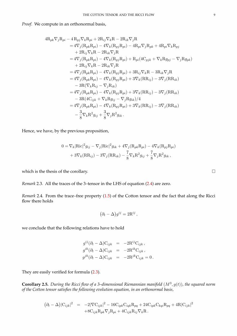
Proof. We compute in an orthonormal basis,
4Rpk∇jRpi − 4 Rpj∇kRpi + 2Rij∇kR− 2Rik∇jR
= 4∇j(RpkRpi)− 4∇k(RpjRpi)− 4Rpi∇jRpk + 4Rpi∇kRpj
+ 2Rij∇kR− 2Rik∇jR
= 4∇j(RpkRpi)− 4∇k(RpjRpi) + Rpi(4Cpjk +∇kRgpj −∇jRgpk)
+ 2Rij∇kR− 2Rik∇jR
= 4∇j(RpkRpi)− 4∇k(RpjRpi) + 3Rij∇kR− 3Rik∇jR
= 4∇j(RpkRpi)− 4∇k(RpjRpi) + 3∇k(RRij)− 3∇j(RRik)
− 3R(∇kRij −∇jRik)
= 4∇j(RpkRpi)− 4∇k(RpjRpi) + 3∇k(RRij)− 3∇j(RRik)
− 3R(4Cijk +∇kRgij −∇jRgik)/4
= 4∇j(RpkRpi)− 4∇k(RpjRpi) + 3∇k(RRij)− 3∇j(RRik)
− 3
8∇kR2gij +
3
8∇jR
2gik .
Hence, we have, by the previous proposition,
0 =∇k|Ric|2gij −∇j |Ric|2gik + 4∇j(RpkRpi)− 4∇k(RpjRpi)
+ 3∇k(RRij)− 3∇j(RRik)− 7
8∇kR2gij +
7
8∇jR
2gik ,
which is the thesis of the corollary. �
Remark 2.3. All the traces of the 3–tensor in the LHS of equation (2.4) are zero.
Remark 2.4. From the trace–free property (1.5) of the Cotton tensor and the fact that along the Ricciflow there holds
(∂t −∆
)gij = 2Rij ,
we conclude that the following relations have to hold
gij(∂t −∆)Cijk = −2RijCijk ,
gik(∂t −∆)Cijk = −2RikCijk ,
gjk(∂t −∆)Cijk = −2RjkCijk = 0 .
They are easily verified for formula (2.3).
Corollary 2.5. During the Ricci flow of a 3–dimensional Riemannian manifold (M3, g(t)), the squared normof the Cotton tensor satisfies the following evolution equation, in an orthonormal basis,
(∂t −∆
)|Cijk|2 = −2|∇Cijk|2 − 16CipkCiqkRpq + 24CipkCkqiRpq + 4R|Cijk|2
+8CijkRpk∇jRpi + 4CijkRij∇kR .

10 CARLO MANTEGAZZA, SAMUELE MONGODI, AND MICHELE RIMOLDI
Proof. (∂t −∆
)|Cijk|2 = −2|∇Cijk|2 + 2CijkRipg
pqCqjk + 2CijkRjpgpqCiqk + 2CijkRkpg
pqCijq
+2Cijk[gpqRpj(Ckqi + Cqki) + 5gpqRipCqkj + gpqRpk(Cjiq + Cqij)
+2RCijk + 2RqlCqjlgik − 2RqlCqklgij
+1
2∇k|Ric|2gij −
1
2∇j |Ric|2gik +
R
2∇jRgik −
R
2∇kRgij
+2gpqRpk∇jRqi − 2gpqRpj∇kRqi + Rij∇kR− Rik∇jR]
= −2|∇Cijk|2 + 2(Ckij + Cjki)Ripgpq(Ckqj + Cjkq)
+2CijkRjpgpqCiqk + 2CikjRkpg
pqCiqj
+2Cijk[2gpqRpj(Ckqi + Cqki) + 5gpqRipCqkj
]+4R|Cijk|2 + 8gpqCijkRpk∇jRqi + 4CijkRij∇kR
= −2|∇Cijk|2 − 16CipkCiqkRpq + 24CipkCkqiRpq + 4R|Cijk|2
+8CijkRpk∇jRpi + 4CijkRij∇kR
where in the last line we assumed to be in a orthonormal basis. �
3. THREE–DIMENSIONAL GRADIENT RICCI SOLITONS
The structural equation of a gradient Ricci soliton (Mn, g,∇f) is the following
(3.1) Rij +∇i∇jf = λgij ,
for some λ ∈ R.The soliton is said to be steady, shrinking or expanding according to the fact that the constant λ is zero,positive or negative, respectively.
It follows that in dimension three, for (M3, g,∇f) there holds
∆Rij = ∇lRij∇lf + 2λRij − 2|Ric|2gij + R2gij − 3RRij + 4RisRsj(3.2)
∆R = ∇lR∇lf + 2λR− 2|Ric|2(3.3)∇iR = 2Rli∇lf(3.4)
Cijk =Rlkgij
2∇lf −
Rljgik2∇lf + Rij∇kf − Rik∇jf +
Rgik2∇jf −
Rgij2∇kf(3.5)
=∇kR
4gij −
∇jR
4gik +
(Rij −
R
2gij
)∇kf −
(Rik −
R
2gik
)∇jf .
In the special case of a steady soliton the first two equations above simplify as follows,
∆Rij = ∇lRij∇lf − 2|Ric|2gij + R2gij − 3RRij + 4RisRsj
∆R = ∇lR∇lf − 2|Ric|2 .
Remark 3.1. We notice that, by relation (3.5), we have
Cijk∇if =∇kR∇jf
4− ∇jR∇kf
4+ Rij∇if∇kf −
R
2∇jf∇kf − Rik∇if∇jf +
R
2∇kf∇jf
=∇jR∇kf
4− ∇kR∇jf
4,
where in the last passage we used relation (3.4).It follows that
Cijk∇if∇jf =〈∇f,∇R〉
4∇kf −
|∇f |2
4∇kR .
Hence, if the Cotton tensor of a three–dimensional gradient Ricci soliton is identically zero, we havethat at every point where∇R is not zero, ∇f and∇R are proportional.
This relation is a key step in (yet another) proof of the fact that a three–dimensional, locally con-formally flat, steady or shrinking gradient Ricci soliton is locally a warped product of a constantcurvature surface on a interval of R, leading to a full classification, first obtained by H.-D. Cao andQ. Chen [4] for the steady case and H.-D. Cao, B.-L. Chen and X.-P. Zhu [3] for the shrinking case
THE COTTON TENSOR AND THE RICCI FLOW 11
(actually this is the last paper of a series finally classifying, in full generality, all the three-dimensionalgradient shrinking Ricci solitons, even without the LCF assumption).
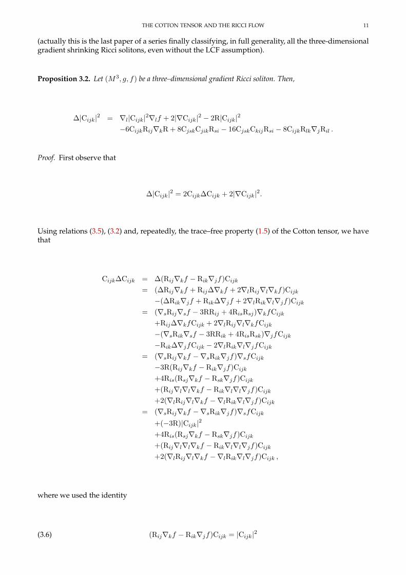
Proposition 3.2. Let (M3, g, f) be a three–dimensional gradient Ricci soliton. Then,
∆|Cijk|2 = ∇l|Cijk|2∇lf + 2|∇Cijk|2 − 2R|Cijk|2
−6CijkRij∇kR + 8CjskCjikRsi − 16CjskCkijRsi − 8CijkRlk∇jRil .
Proof. First observe that
∆|Cijk|2 = 2Cijk∆Cijk + 2|∇Cijk|2.
Using relations (3.5), (3.2) and, repeatedly, the trace–free property (1.5) of the Cotton tensor, we havethat
Cijk∆Cijk = ∆(Rij∇kf − Rik∇jf)Cijk
= (∆Rij∇kf + Rij∆∇kf + 2∇lRij∇l∇kf)Cijk
−(∆Rik∇jf + Rik∆∇jf + 2∇lRik∇l∇jf)Cijk
= (∇sRij∇sf − 3RRij + 4RisRsj)∇kfCijk
+Rij∆∇kfCijk + 2∇lRij∇l∇kfCijk
−(∇sRik∇sf − 3RRik + 4RisRsk)∇jfCijk
−Rik∆∇jfCijk − 2∇lRik∇l∇jfCijk
= (∇sRij∇kf −∇sRik∇jf)∇sfCijk
−3R(Rij∇kf − Rik∇jf)Cijk
+4Ris(Rsj∇kf − Rsk∇jf)Cijk
+(Rij∇l∇l∇kf − Rik∇l∇l∇jf)Cijk
+2(∇lRij∇l∇kf −∇lRik∇l∇jf)Cijk
= (∇sRij∇kf −∇sRik∇jf)∇sfCijk
+(−3R)|Cijk|2
+4Ris(Rsj∇kf − Rsk∇jf)Cijk
+(Rij∇l∇l∇kf − Rik∇l∇l∇jf)Cijk
+2(∇lRij∇l∇kf −∇lRik∇l∇jf)Cijk ,
where we used the identity
(3.6) (Rij∇kf − Rik∇jf)Cijk = |Cijk|2

12 CARLO MANTEGAZZA, SAMUELE MONGODI, AND MICHELE RIMOLDI
which follows easily by equation (3.5) and the fact that every trace of the Cotton tensor is zero.Using now equations (3.1), (3.5), (1.5), (1.4), and (3.4), we compute
(∇sRij∇kf −∇sRik∇jf)∇sfCijk = (∇s(Rij∇kf)− Rij∇s∇kf)∇sfCijk
−(∇s(Rik∇jf)− Rik∇s∇jf)∇sfCijk
= (∇s(Rij∇kf − Rik∇jf) + Rij(Rsk))∇sfCijk
−(Rik(Rsj))∇sfCijk
= ∇sCijkCijk∇sf + RijRsk∇sfCijk − RikRsj∇sfCijk
=1
2∇s|Cijk|2∇sf +
1
2Rij∇kRCijk −
1
2Rik∇jRCijk
4Ris(Rsj∇kf − Rsk∇jf)Cijk = 4Ris(Csjk −1
4∇kRgsj +
1
4∇jRgsk +
R
2∇kfgsj −
R
2∇jfgsk)Cijk
= 4Ris(−Cjks − Cksj)(−Cjki − Ckij)− Rij∇kRCijk
+Rik∇jRCijk + 2RRij∇kfCijk − 2RRik∇jfCijk
= 8RisCjskCjik − 8RisCjskCkij
−Rij∇kRCijk + Rik∇jRCijk + 2R|Cijk|2
(Rij∇l∇l∇kf − Rik∇l∇l∇jf)Cijk = (Rij∇l(−Rlk)− Rik∇l(−Rlj))Cijk
= −1
2Rij∇kRCijk +
1
2Rik∇jRCijk
2(∇lRij∇l∇kf −∇lRik∇l∇jf)Cijk = 2((Cijl +∇jRil +1
4∇lRgij −
1
4∇jRgil)(−Rlk))Cijk
−2((Cikl +∇kRil +1
4∇lRgik −
1
4∇kRgil)(−Rlj))Cijk
= −2CijlCijkRlk − 2CijkRlk∇jRil +1
2CijkRik∇jR
+2CiklCijkRlj + 2CijkRlj∇kRil −1
2CijkRij∇kR
= −2CiljCikjRlk − 2CijkRlk∇jRil +1
2CijkRik∇jR
−2CilkCijkRlj + 2CijkRlj∇kRil −1
2CijkRij∇kR.
Hence, getting back to the main computation and using again the symmetry relations (1.4), we finallyget
Cijk∆Cijk =1
2∇s|Cijk|2∇sf − R|Cijk|2
−3
2CijkRij∇kR +
3
2CijkRik∇jR
+4CjskCjikRsi − 8CjskCkijRsi
−2CijkRlk∇jRil + 2CijkRlj∇kRil
=1
2∇s|Cijk|2∇sf − R|Cijk|2
−3CijkRij∇kR + 4CjskCjikRsi − 8CjskCkijRsi − 4CijkRlk∇jRil
where in the last passage we applied the skew–symmetry of the Cotton tensor in its last two indexes.The thesis follows. �

THE COTTON TENSOR AND THE RICCI FLOW 13
4. THE EVOLUTION EQUATION OF THE COTTON TENSOR IN ANY DIMENSION
In this section we will compute the evolution equation under the Ricci flow of the Cotton tensorCijk, for every n–dimensional Riemannian manifold (Mn, g(t)) evolving by Ricci flow.
Among the evolution equations (1.6) we expand the one for the Ricci tensor,
∂
∂tRij = ∆Rij −
2n
n− 2gpqRipRjq +
2n
(n− 1)(n− 2)RRij +
2
n− 2|Ric|2gij
− 2
(n− 1)(n− 2)R2gij − 2RpqWpijq .
Then, we compute the evolution equations of the derivatives of the curvatures assuming, from nowon, to be in normal coordinates,
∂
∂t∇lR = ∇l∆R + 2∇l|Ric|2 ,
∂
∂t∇sRij = ∇s∆Rij −
2n
n− 2∇sRipRjp −
2n
n− 2Rip∇sRjp +
2n
(n− 1)(n− 2)∇sRRij
+2n
(n− 1)(n− 2)R∇sRij +
2
n− 2∇s|Ric|2gij −
2
(n− 1)(n− 2)∇sR
2gij
−2∇sRklWkijl − 2Rkl∇sWkijl + (∇iRsp +∇sRip −∇pRis)Rjp
+(∇jRsp +∇sRjp −∇pRjs)Rip
= ∇s∆Rij −n+ 2
n− 2∇sRipRjp −
n+ 2
n− 2Rip∇sRjp +
2n
(n− 1)(n− 2)∇sRRij
+2n
(n− 1)(n− 2)R∇sRij +
2
n− 2∇s|Ric|2gij −
2
(n− 1)(n− 2)∇sR
2gij
−2∇sRklWkijl − 2Rkl∇sWkijl + (∇iRsp −∇pRis)Rjp + (∇jRsp −∇pRjs)Rip
= ∇s∆Rij −n+ 2
n− 2∇sRipRjp −
n+ 2
n− 2Rip∇sRjp +
2n
(n− 1)(n− 2)∇sRRij
+2n
(n− 1)(n− 2)R∇sRij +
2
n− 2∇s|Ric|2gij −
2
(n− 1)(n− 2)∇sR
2gij
−2∇sRklWkijl − 2Rkl∇sWkijl + CspiRjp + CspjRip
+1
2(n− 1)Rjp[∇iRgsp −∇pRgis] +
1
2(n− 1)Rip[∇jRgsp −∇pRgjs] ,
where in the last passage we substituted the expression of the Cotton tensor.

14 CARLO MANTEGAZZA, SAMUELE MONGODI, AND MICHELE RIMOLDI
We then compute,
∂
∂tCijk =
∂
∂t∇kRij −
∂
∂t∇jRik −
1
2(n− 1)
∂
∂t
(∇kRgij −∇jRgik
)= ∇k∆Rij −
n+ 2
n− 2∇kRipRjp −
n+ 2
n− 2Rip∇kRjp +
2n
(n− 1)(n− 2)∇kRRij
+2n
(n− 1)(n− 2)R∇kRij +
2
n− 2∇k|Ric|2gij −
2
(n− 1)(n− 2)∇kR2gij
−2∇kRplWpijl − 2Rpl∇kWpijl + CkpiRjp + CkpjRip
+Rjp
2(n− 1)[∇iRgkp −∇pRgik] +
Rip
2(n− 1)[∇jRgkp −∇pRgjk]
−∇j∆Rik +n+ 2
n− 2∇jRipRkp +
n+ 2
n− 2Rip∇jRkp −
2n
(n− 1)(n− 2)∇jRRik
− 2n
(n− 1)(n− 2)R∇jRik −
2
n− 2∇j |Ric|2gik +
2
n− 1∇jR
2gik
−2∇kRplWpijl − 2Rpl∇kWpijl − CjpiRkp − CjpkRip
−Rkp
2(n− 1)[∇iRgjp −∇pRgij ]−
Rip
2(n− 1)[∇kRgjp −∇pRgkj ]
+1
n− 1(Rij∇kR− Rik∇jR
)−(∇k∆R + 2∇k|Ric|2
) gij2(n− 1)
+(∇j∆R + 2∇j |Ric|2
) gik2(n− 1)
= ∇k∆Rij −n+ 2
n− 2∇kRipRjp −
n+ 2
n− 2Rip∇kRjp
+5n− 2
2(n− 1)(n− 2)∇kRRij +
2n
(n− 1)(n− 2)R∇kRij
+n
(n− 1)(n− 2)∇k|Ric|2gij −
2
(n− 1)(n− 2)∇kR2gij
+CkpiRjp + CkpjRip − 2∇kRplWpijl − 2Rpl∇kWpijl
− 1
2(n− 1)Rpj∇pRgik
−∇j∆Rik +n+ 2
n− 2∇jRipRkp +
n+ 2
n− 2Rip∇jRkp
− 5n− 2
2(n− 1)(n− 2)∇jRRik −
2n
(n− 1)(n− 2)R∇jRik
− n
(n− 1)(n− 2)∇j |Ric|2gik +
2
(n− 1)(n− 2)∇jR
2gik
−CjpiRkp − CjpkRip + 2∇jRplWpikl + 2Rpl∇jWpikl
+1
2(n− 1)∇lRRlkgij −
1
2(n− 1)∇k∆Rgij +
1
2(n− 1)∇j∆Rgik
and
∆Cijk = ∆∇kRij −∆∇jRik −1
2(n− 1)∆∇kRgij +
1
2(n− 1)∆∇jRgik ,

THE COTTON TENSOR AND THE RICCI FLOW 15
hence,
∂
∂tCijk −∆Cijk = ∇k∆Rij −∇j∆Rik −∆∇kRij + ∆∇jRik
− 1
2(n− 1)(∇k∆Rgij −∇j∆Rgik −∆∇kRgij + ∆∇jRgik)
−n+ 2
n− 2(∇kRipRjp + Rip∇kRjp) +
5n− 2
2(n− 1)(n− 2)∇kRRij
+2n
(n− 1)(n− 2)R∇kRij
+n
(n− 1)(n− 2)∇k|Ric|2gij −
2
(n− 1)(n− 2)∇kR2gij
+CkpiRjp + CkpjRip − 2∇kRplWpijl − 2Rpl∇kWpijl
− 1
2(n− 1)Rjp∇pRgik
+n+ 2
n− 2(∇jRipRkp + Rip∇jRkp)−
5n− 2
2(n− 1)(n− 2)∇jRRik
− 2n
(n− 1)(n− 2)R∇jRik
− n
(n− 1)(n− 2)∇j |Ric|2gik +
2
(n− 1)(n− 2)∇jR
2gik
−CjpiRkp − CjpkRip + 2∇jRplWpikl + 2Rpl∇jWpikl
+1
2(n− 1)Rkp∇pRgij
Now to proceed, we need the following commutation rules for the derivatives of the Ricci ten-sor and of the scalar curvature, where we will employ the decomposition formula of the Riemann
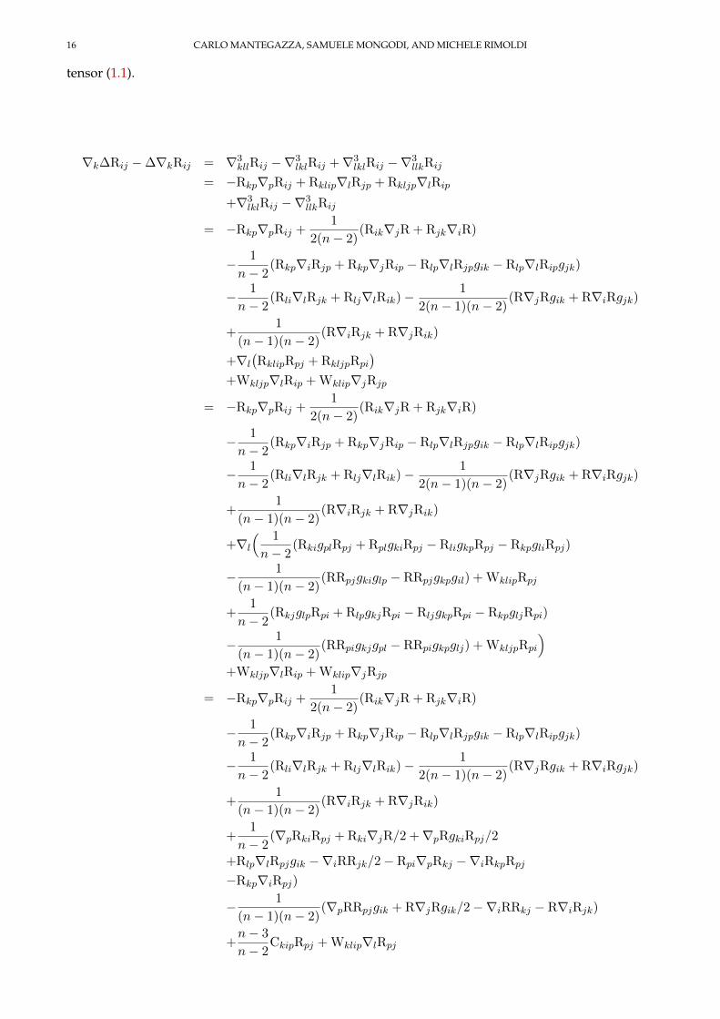
16 CARLO MANTEGAZZA, SAMUELE MONGODI, AND MICHELE RIMOLDI
tensor (1.1).
∇k∆Rij −∆∇kRij = ∇3kllRij −∇3
lklRij +∇3lklRij −∇3
llkRij
= −Rkp∇pRij + Rklip∇lRjp + Rkljp∇lRip
+∇3lklRij −∇3
llkRij
= −Rkp∇pRij +1
2(n− 2)(Rik∇jR + Rjk∇iR)
− 1
n− 2(Rkp∇iRjp + Rkp∇jRip − Rlp∇lRjpgik − Rlp∇lRipgjk)
− 1
n− 2(Rli∇lRjk + Rlj∇lRik)− 1
2(n− 1)(n− 2)(R∇jRgik + R∇iRgjk)
+1
(n− 1)(n− 2)(R∇iRjk + R∇jRik)
+∇l
(RklipRpj + RkljpRpi
)+Wkljp∇lRip + Wklip∇jRjp
= −Rkp∇pRij +1
2(n− 2)(Rik∇jR + Rjk∇iR)
− 1
n− 2(Rkp∇iRjp + Rkp∇jRip − Rlp∇lRjpgik − Rlp∇lRipgjk)
− 1
n− 2(Rli∇lRjk + Rlj∇lRik)− 1
2(n− 1)(n− 2)(R∇jRgik + R∇iRgjk)
+1
(n− 1)(n− 2)(R∇iRjk + R∇jRik)
+∇l
( 1
n− 2(RkigplRpj + RplgkiRpj − RligkpRpj − RkpgliRpj)
− 1
(n− 1)(n− 2)(RRpjgkiglp − RRpjgkpgil) + WklipRpj
+1
n− 2(RkjglpRpi + RlpgkjRpi − RljgkpRpi − RkpgljRpi)
− 1
(n− 1)(n− 2)(RRpigkjgpl − RRpigkpglj) + WkljpRpi
)+Wkljp∇lRip + Wklip∇jRjp
= −Rkp∇pRij +1
2(n− 2)(Rik∇jR + Rjk∇iR)
− 1
n− 2(Rkp∇iRjp + Rkp∇jRip − Rlp∇lRjpgik − Rlp∇lRipgjk)
− 1
n− 2(Rli∇lRjk + Rlj∇lRik)− 1
2(n− 1)(n− 2)(R∇jRgik + R∇iRgjk)
+1
(n− 1)(n− 2)(R∇iRjk + R∇jRik)
+1
n− 2(∇pRkiRpj + Rki∇jR/2 +∇pRgkiRpj/2
+Rlp∇lRpjgik −∇iRRjk/2− Rpi∇pRkj −∇iRkpRpj
−Rkp∇iRpj)
− 1
(n− 1)(n− 2)(∇pRRpjgik + R∇jRgik/2−∇iRRkj − R∇iRjk)
+n− 3
n− 2CkipRpj + Wklip∇lRpj
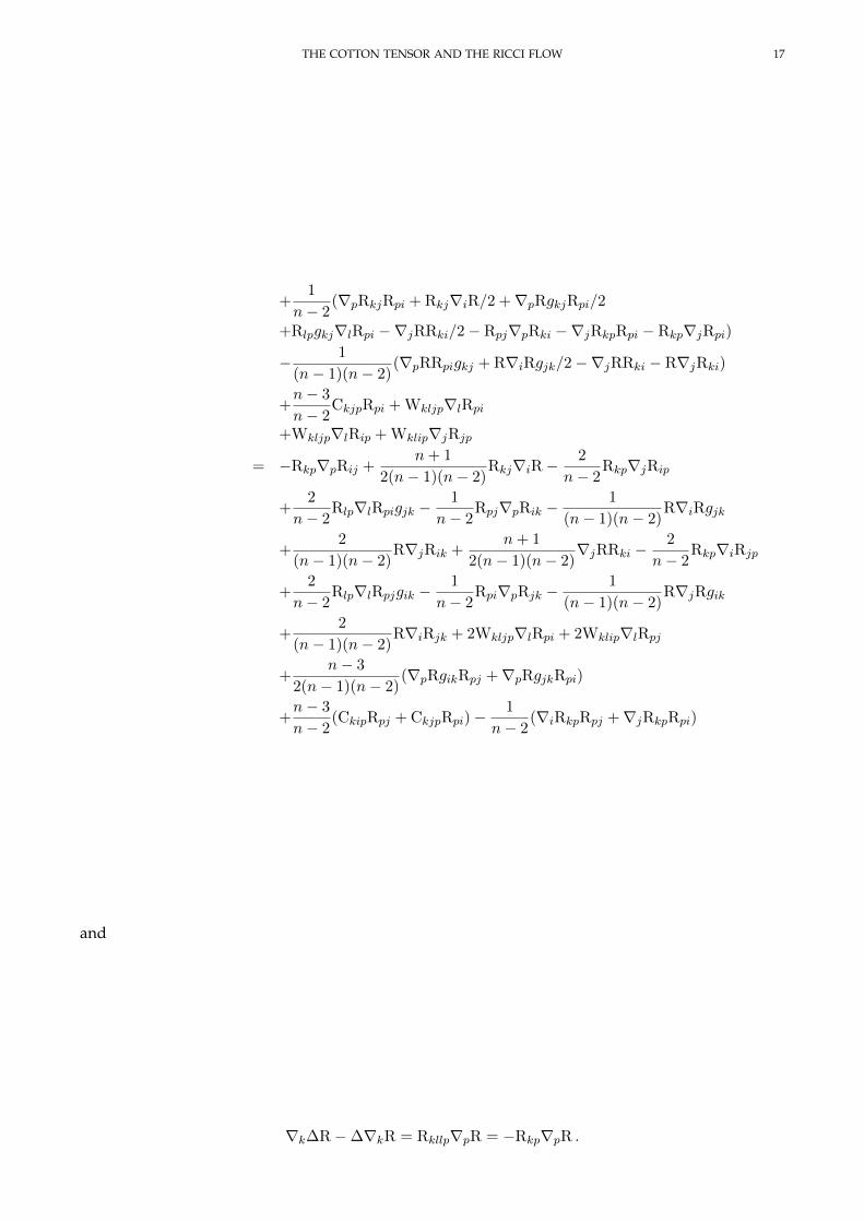
THE COTTON TENSOR AND THE RICCI FLOW 17
+1
n− 2(∇pRkjRpi + Rkj∇iR/2 +∇pRgkjRpi/2
+Rlpgkj∇lRpi −∇jRRki/2− Rpj∇pRki −∇jRkpRpi − Rkp∇jRpi)
− 1
(n− 1)(n− 2)(∇pRRpigkj + R∇iRgjk/2−∇jRRki − R∇jRki)
+n− 3
n− 2CkjpRpi + Wkljp∇lRpi
+Wkljp∇lRip + Wklip∇jRjp
= −Rkp∇pRij +n+ 1
2(n− 1)(n− 2)Rkj∇iR−
2
n− 2Rkp∇jRip
+2
n− 2Rlp∇lRpigjk −
1
n− 2Rpj∇pRik −
1
(n− 1)(n− 2)R∇iRgjk
+2
(n− 1)(n− 2)R∇jRik +
n+ 1
2(n− 1)(n− 2)∇jRRki −
2
n− 2Rkp∇iRjp
+2
n− 2Rlp∇lRpjgik −
1
n− 2Rpi∇pRjk −
1
(n− 1)(n− 2)R∇jRgik
+2
(n− 1)(n− 2)R∇iRjk + 2Wkljp∇lRpi + 2Wklip∇lRpj
+n− 3
2(n− 1)(n− 2)(∇pRgikRpj +∇pRgjkRpi)
+n− 3
n− 2(CkipRpj + CkjpRpi)−
1
n− 2(∇iRkpRpj +∇jRkpRpi)
and
∇k∆R−∆∇kR = Rkllp∇pR = −Rkp∇pR .

18 CARLO MANTEGAZZA, SAMUELE MONGODI, AND MICHELE RIMOLDI
Then, getting back to the main computation, we obtain
∂
∂tCijk −∆Cijk = −Rkp∇pRij +
n+ 1
2(n− 1)(n− 2)Rkj∇iR
− 2
n− 2Rkp∇jRip +
2
n− 2Rlp∇lRpigjk
− 1
n− 2Rjp∇pRik −
1
(n− 1)(n− 2)R∇iRgjk
+2
(n− 1)(n− 2)R∇jRik +
n+ 1
2(n− 1)(n− 2)∇jRRki
− 2
n− 2Rkp∇iRpj +
2
n− 2Rlp∇lRpjgik
− 1
n− 2Rpi∇pRkj −
1
(n− 1)(n− 2)R∇jRgik
+2
(n− 1)(n− 2)R∇iRjk + 2Wkljp∇lRpi + 2Wklip∇lRpj
+n− 3
2(n− 1)(n− 2)(∇pRgikRpj +∇pRgjkRpi)
+n− 3
n− 2(CkipRpj + CkjpRpi)
− 1
n− 2(∇iRkpRjp +∇jRkpRpi)
+Rjp∇pRik −n+ 1
2(n− 1)(n− 2)Rkj∇iR +
2
n− 2Rjp∇kRip
− 2
n− 2Rlp∇lRpigkj +
1
n− 2Rpk∇pRij
+1
(n− 1)(n− 2)R∇iRgjk −
2
(n− 1)(n− 2)R∇kRij
− n+ 1
2(n− 1)(n− 2)∇kRRij +
2
n− 2Rjp∇iRkp
− 2
n− 2Rlp∇pRpkgij +
1
n− 2Rpi∇pRkj
+1
(n− 1)(n− 2)R∇kRgij −
2
(n− 1)(n− 2)R∇iRkj
−2Wjlkp∇lRpi − 2Wjlip∇lRpk
− n− 3
2(n− 2)(n− 2)(∇pRgijRpk +∇pRgjkRpi)
−n− 3
n− 2(CjipRpk + CjkpRpi) +
1
n− 2(∇iRpjRpk +∇kRjpRpi)
+1
2(n− 1)(Rkp∇pRgij − Rjp∇pRgki)−
n+ 2
n− 2(∇kRpiRpj + Rpi∇kRpj)
+n
(n− 1)(n− 2)∇k|Ric|2gij +
5n− 2
2(n− 1)(n− 2)∇kRRij
+2n
(n− 1)(n− 2)R∇kRij −
2
(n− 1)(n− 2)∇kR2gij
−2∇kRplWpijl − 2Rpl∇kWpijl
+CkliRlj −1
2(n− 1)∇lRRljgik + CkljRli

THE COTTON TENSOR AND THE RICCI FLOW 19
+n+ 2
n− 2(∇jRpiRpk + Rpi∇jRpk)
− n
(n− 1)(n− 2)∇j |Ric|2gki −
5n− 2
2(n− 1)(n− 2)∇jRRik
− 2n
(n− 1)(n− 2)R∇jRik +
2
(n− 1)(n− 2)∇jR
2gik
+2∇jRplWpikl + 2Rpl∇jWpikl
−CjliRlk +1
2(n− 1)∇lRRlkgij − CjlkRli
=1
n− 2(RpiCjkp + RpkCjip − CkipRpj − CkjpRpi)
+[ 2
n− 2Rlp∇lRpj +
3
2(n− 1)(n− 2)∇jR
2
− 1
2(n− 2)∇pRRpj −
n
(n− 1)(n− 2)∇j |Ric|2
]gik
−[ 2
n− 2Rlp∇lRpk +
3
2(n− 1)(n− 2)∇kR2
− 1
2(n− 2)∇pRRpk −
n
(n− 1)(n− 2)∇k|Ric|2
]gij
−n− 3
n− 2Rkp∇pRij +
n− 3
n− 2Rpj∇pRik
+n
n− 2Rkp∇jRpi +
n+ 1
n− 2∇jRpkRpi −
2
n− 2R∇jRik
− 4n− 3
2(n− 1)(n− 2)∇jRRik −
1
n− 2Rkp∇iRpj +
1
n− 2Rpj∇iRpk
− n
n− 2Rjp∇kRip −
n+ 1
n− 2∇kRjpRip +
2
n− 2R∇kRij
+4n− 3
2(n− 1)(n− 2)∇kRRij + 2Wklip∇lRpj + 2Wkljp∇lRpi − 2Wjlkp∇lRpi
−2Wjlip∇lRpk − 2∇kRplWpijl − 2Rpl∇kWpijl + 2∇jRplWpikl + 2Rpl∇jWpikl
Now, by means of the very definition of the Cotton tensor (1.2), the identities (1.4), and the symme-tries of the Weyl tensor, we substitute
Ckpj − Cjpk = − Ckjp − Cjpk = Cpkj
∇lRjp =∇jRlp + Cpjl +1
2(n− 1)
(∇lRgpj −∇jRgpl
)∇lRkp =∇kRlp + Cpkl +
1
2(n− 1)
(∇lRgpk −∇kRgpl
)∇iRjp =∇jRip + Cpji +
1
2(n− 1)
(∇iRgjp −∇jRgip
)∇iRkp =∇kRip + Cpki +
1
2(n− 1)
(∇iRgkp −∇kRgip
)∇pRij =∇jRpi + Cijp +
1
2(n− 1)
(∇pRgji −∇jRgpi
)∇pRik =∇kRpi + Cikp +
1
2(n− 1)
(∇pRgki −∇kRgpi
)

20 CARLO MANTEGAZZA, SAMUELE MONGODI, AND MICHELE RIMOLDI
in the last expression above, getting
∂
∂tCijk −∆Cijk =
1
n− 2(RpiCpkj + RpkCjip − CkipRpj)
+[ 2
n− 2Rlp
(∇jRlp + Cpjl +
1
2(n− 1)∇lRgpj
− 1
2(n− 1)∇jRgpl)
)+
3
2(n− 1)(n− 2)∇jR
2
− 1
2(n− 2)∇pRRpj −
n
(n− 1)(n− 2)∇j |Ric|2
]gik
−[ 2
n− 2Rlp
(∇kRpl + Cpkl +
1
2(n− 1)∇lRgpk
− 1
2(n− 1)∇kRgpl
)+
3
2(n− 1)(n− 2)∇kR2
− 1
2(n− 2)∇pRRpk −
n
(n− 1)(n− 2)∇k|Ric|2
]gij
−n− 3
n− 2Rkp
(Cijp +∇jRip +
1
2(n− 1)(∇pRgij −∇jRgip)
)+n− 3
n− 2Rpj
(Cikp +∇kRip +
1
2(n− 1)(∇pRgik −∇kRgip)
)+
n
n− 2Rkp∇jRpi +
n+ 1
n− 2∇jRpkRpi −
2
n− 2R∇jRik
− 4n− 3
2(n− 1)(n− 2)∇jRRik
− 1
n− 2Rkp
(∇jRip + Cpji +
1
2(n− 1)(∇iRgjp −∇jRgip)
)+
1
n− 2Rpj
(∇kRip + Ckpi +
1
2(n− 1)(∇iRgkp −∇kRgip)
)− n
n− 2Rjp∇kRip −
n+ 1
n− 2∇kRjpRip +
2
n− 2R∇kRij
+4n− 3
2(n− 1)(n− 2)∇kRRij
+2CpljWpikl − 2CplkWpijl − 2CpilWjklp
−2Wjklp∇iRpl − 2Rpl∇kWpijl + 2Rpl∇jWpikl
=1
n− 2(RpiCpkj + Rpk(Cjip − Cpji − (n− 3)Cijp) + Rpj(Cpki − Ckip + (n− 3)Cikp))
+2
n− 2CpjlRplgik −
2
n− 2CpklRplgij − 2CpjlWpikl + 2CpklWpijl − 2CpilWjklp
+gik
[ ∇jR2
(n− 1)(n− 2)− 1
(n− 1)(n− 2)∇j |Ric|2
]−gij
[ ∇kR2
(n− 1)(n− 2)− 1
(n− 1)(n− 2)∇k|Ric|2
]− 2
n− 2Rjp∇kRip −
n+ 1
n− 2∇kRjpRip +
3n− 1
2(n− 1)(n− 2)∇kRRij +
2
n− 2R∇kRij
+2
n− 2Rkp∇jRip +
n+ 1
n− 2∇jRkpRip −
3n− 1
2(n− 1)(n− 2)∇jRRik −
2
n− 2R∇jRik
−2Wjklp∇iRlp − 2Rlp∇kWpijl + 2Rpl∇jWpikl .

THE COTTON TENSOR AND THE RICCI FLOW 21
then, we substitute again
∇kRjp =∇pRkj + Cjpk +1
2(n− 1)
(∇kRgjp −∇pRgjk
)∇jRkp =∇pRjk + Ckpj +
1
2(n− 1)
(∇jRgkp −∇pRgkj
)∇kRij =∇iRkj + Cjik +
1
2(n− 1)
(∇kRgij −∇iRgjk
)∇jRik =∇iRjk + Ckij +
1
2(n− 1)
(∇jRgik −∇iRgkj
),
finally obtaining
∂
∂tCijk −∆Cijk =
1
n− 2(RpiCpkj + Rpk(Cjip − Cpji − (n− 3)Cijp) + Rpj(Cpki − Ckip + (n− 3)Cikp))
+2
n− 2CpjlRplgik −
2
n− 2CpklRplgij − 2CpjlWpikl + 2CpklWpijl − 2CpilWjklp
+gik
[ ∇jR2
(n− 1)(n− 2)− 1
(n− 1)(n− 2)∇j |Ric|2
]−gij
[ ∇kR2
(n− 1)(n− 2)− 1
(n− 1)(n− 2)∇k|Ric|2
]− 2
n− 2Rjp∇kRip −
n+ 1
n− 2Rip∇pRkj −
n+ 1
n− 2RipCjpk
− n+ 1
2(n− 1)(n− 2)Rij∇kR +
n+ 1
2(n− 1)(n− 2)Rip∇pRgjk
+3n− 1
2(n− 1)(n− 2)∇kRRij +
2
n− 2R(∇iRjk + Cjik +
1
2(n− 1)(∇kRgij −∇iRgjk))
+2
n− 2Rkp∇jRip +
n+ 1
n− 2Rip∇pRkj +
n+ 1
n− 2RipCkpj +
n+ 1
2(n− 1)(n− 2)∇jRRik
− n+ 1
2(n− 1)(n− 2)Rip∇pRgjk −
3n− 1
2(n− 1)(n− 2)∇jRRik
− 2
n− 2R(∇iRjk + Ckij +
1
2(n− 1)(∇jRgik −∇iRgjk))
−2Wjklp∇iRlp − 2Rlp∇kWpijl + 2Rpl∇jWpikl
=1
n− 2(Rpk(Cjip − Cpji − (n− 3)Cijp)− Rpj(Ckip − Cpki − (n− 3)Cikp)
+(n+ 2)RpiCpkj) +2
n− 2(CpjlRplgik − CpklRplgij) +
2
n− 2RCijk
−2WpiklCpjl + 2WpijlCpkl − 2CpilWjklp
+gik
[ ∇jR2
2(n− 1)(n− 2)− 1
(n− 1)(n− 2)∇j |Ric|2
]−gij
[ ∇kR2
2(n− 1)(n− 2)− 1
(n− 1)(n− 2)∇k|Ric|2
]− 2
n− 2Rjp∇kRip +
1
n− 2∇kRRij
+2
n− 2Rkp∇jRip −
1
n− 2∇jRRik
+2Rlp∇jWpikl − 2Rlp∇kWpijl ,
where in the last passage we used again the identities (1.4) and the fact that
Wjklp∇iRlp = Wjkpl∇iRpl = Wjkpl∇iRlp = −Wjklp∇iRlp .
Hence, we can resume this long computation in the following proposition, getting back to a genericcoordinate basis.

22 CARLO MANTEGAZZA, SAMUELE MONGODI, AND MICHELE RIMOLDI
Proposition 4.1. During the Ricci flow of a n–dimensional Riemannian manifold (Mn, g(t)), the Cottontensor satisfies the following evolution equation
(∂t −∆
)Cijk =
1
n− 2[gpqRpj(Ckqi + Cqki + (n− 3)Cikq)
+(n+ 2)gpqRipCqkj − gpqRpk(Cjqi + Cqji + (n− 3)Cijq)]
+2
n− 2RCijk +
2
n− 2RqlCqjlgik −
2
n− 2RqlCqklgij
+1
(n− 1)(n− 2)∇k|Ric|2gij −
1
(n− 1)(n− 2)∇j |Ric|2gik
+R
(n− 1)(n− 2)∇jRgik −
R
(n− 1)(n− 2)∇kRgij
+2
n− 2gpqRpk∇jRqi −
2
n− 2gpqRpj∇kRqi +
1
n− 2Rij∇kR− 1
n− 2Rik∇jR
−2gpqWpiklCqjl + 2gpqWpijlCqkl − 2gpqWjklpCqil + 2gpqRpl∇jWqikl − 2gpqRpl∇kWqijl .
In particular if the Cotton tensor vanishes identically along the flow we obtain,
0 =1
(n− 1)(n− 2)∇k|Ric|2gij −
1
(n− 1)(n− 2)∇j |Ric|2gik
+R
(n− 1)(n− 2)∇jRgik −
R
(n− 1)(n− 2)∇kRgij
+2
n− 2gpqRpk∇jRqi −
2
n− 2gpqRpj∇kRqi +
1
n− 2Rij∇kR− 1
n− 2Rik∇jR
+2gpqRpl∇jWqikl − 2gpqRpl∇kWqijl ,
while, in virtue of relation (1.3), if the Weyl tensor vanishes along the flow we obtain (compare with [5, Propo-sition 1.1 and Corollary 1.2])
0 =1
(n− 1)(n− 2)∇k|Ric|2gij −
1
(n− 1)(n− 2)∇j |Ric|2gik
+R
(n− 1)(n− 2)∇jRgik −
R
(n− 1)(n− 2)∇kRgij
+2
n− 2gpqRpk∇jRqi −
2
n− 2gpqRpj∇kRqi +
1
n− 2Rij∇kR− 1
n− 2Rik∇jR .
Corollary 4.2. During the Ricci flow of a n–dimensional Riemannian manifold (Mn, g(t)), the squared normof the Cotton tensor satisfies the following evolution equation, in an orthonormal basis,
(∂t −∆
)|Cijk|2 = −2|∇Cijk|2 −
16
n− 2CipkCiqkRpq +
24
n− 2CipkCkqiRpq
+4
n− 2R|Cijk|2 +
8
n− 2CijkRpk∇jRpi +
4
n− 2CijkRij∇kR
+8CijkRlp∇jWpikl − 8CijkCpjlWpikl − 4CjpiCljkWpikl .

THE COTTON TENSOR AND THE RICCI FLOW 23
(∂t −∆
)|Cijk|2 = −2|∇Cijk|2 + 2CijkRipg
pqCqjk + 2CijkRjpgpqCiqk + 2CijkRkpg
pqCiqk
+2Cijk
[ 1
n− 2[(Rpj(Ckpi + Cpki + (n− 3)Cikp)
+(n+ 2)RpiCpkj − Rpk(Cjpi + Cpji + (n− 3)Cijp))
+2
n− 2RCijk +
2
n− 2RqlCqjlgik −
2
n− 2RqlCqklgij
+1
(n− 1)(n− 2)∇k|Ric|2gij −
1
(n− 1)(n− 2)∇j |Ric|2gik
+R
(n− 1)(n− 2)∇jRgik −
R
(n− 1)(n− 2)∇kRgij
+2
n− 2Rqk∇jRqi −
2
n− 2Rqj∇kRqi +
1
n− 2Rij∇kR− 1
n− 2Rik∇jR
−2WpiklCpjl + 2WpijlCpkl − 2WjklpCpil + 2Rpl∇jWpikl − 2Rpl∇kWpikl
]= −2|∇Cijk|2 −
16
n− 2CipkCiqkRpq +
24
n− 2CipkCkqiRpq
+4
n− 2R|Cijk|2 +
8
n− 2CijkRpk∇jRpi +
4
n− 2CijkRij∇kR
+8CijkRlp∇jWpikl − 8CijkCpjlWpikl − 4CjpiCljkWpikl .
Remark 4.3. Notice that if n = 3 the two formulas in Proposition 4.1 and Corollary 4.2 become the onesin Proposition 2.1 and Corollary 2.5.
5. THE BACH TENSOR
The Bach tensor in dimension three is given by
Bik = ∇jCijk .
Let Sij = Rij − 12(n−1)Rgij be the Schouten tensor, then
(5.1) Bik = ∇jCijk = ∇j(∇kSij −∇jSik) = ∇j∇kSij −∆Sik .
We compute, in generic dimension n,
∇jCijk = ∇j∇kRij −1
2(n− 1)∇j∇kRgij −∆Sik
= +RjkilRjl + RjkjlRil +∇k∇jRij −1
2(n− 1)∇k∇jRgij −∆Sik
= +1
n− 2
(Rijgkl − Rjlgki + Rklgij − Rkigjl −
R
(n− 1)(gijgkl − gjlgki)
)Rjl + WjkilRjl
+RklRil +1
2∇k∇iR−
1
2(n− 1)∇k∇iR−∆Sik
= +1
n− 2(RjiRjk − |Ric|2gik + RklRil − RRik)− R
(n− 1)(n− 2)Rik +
R2
(n− 1)(n− 2)gik
+WjkilRjl + RklRil +n− 2
2(n− 1)∇k∇iR−∆Sik
=n
n− 2RijRkj −
n
(n− 1)(n− 2)RRik −
1
n− 2|Ric|2gik +
R2
(n− 1)(n− 2)gik
+WjkilRjl +n− 2
2(n− 1)∇k∇iR−∆Sik .
From this last expression, it is easy to see that the Bach tensor in dimension 3 is symmetric, i.e. Bik =Bki. Moreover, it is trace–free, that is, gikBik = 0 as gik∇Cijk = 0.

24 CARLO MANTEGAZZA, SAMUELE MONGODI, AND MICHELE RIMOLDI
Remark 5.1. In higher dimension, the Bach tensor is given by
Bik =1
n− 2(∇jCijk − RjlWijkl) .
We note that, since RjlWijkl = RjlWklij = RjlWkjil, from the above computation we get that the Bachtensor is symmetric in any dimension; finally, as the Weyl tensor is trace-free in every pair of indexes,there holds gikBik = 0.
We recall that Schur lemma yields the following equation for the divergence of the Schouten tensor
(5.2) ∇jSij =n− 2
2(n− 1)∇iR .
We write∇k∇jCijk = ∇k∇j∇kSij −∇k∇j∇jSik = [∇j ,∇k]∇jSik ,
therefore,
∇k∇jCijk = Rjkjl∇lSik + Rjkil∇jSlk + Rjkkl∇jSli
= Rkl∇lSik + Rjkil∇jSlk − Rjl∇jSli
=
[1
n− 2(Rijgkl − Rjlgik + Rklgij − Rikgjl)−
1
(n− 1)(n− 2)R(gijgkl − gikgjl) + Wjkil
]∇jSlk
=1
n− 2(−Rjl∇jSil + Rkl∇iSkl) + Wjkil∇jSlk
=1
n− 2Rjl(∇iSlj −∇jSil) + Wjkil∇jRkl
=1
n− 2RjlClji + Wiljk∇jRkl ,
where we repeatedly used equation (5.2), the trace–free property of the Weyl tensor and the definitionof the Cotton tensor.
Recalling that
∇kWijkl = ∇kWklij = −n− 3
n− 2Clij =
n− 3
n− 2Clji ,
the divergence of the Bach tensor is given by
∇kBik =1
n− 2∇k(∇jCijk − RjlWijkl) =
1
(n− 2)2RjlCjli −
n− 3
(n− 2)2CjliRjl
= − n− 4
(n− 2)2CjliRjl .
In particular, for n = 3, we obtain ∇kBik = ∇kBki = RjlCjli and, for n = 4, we get the classical result∇kBik = ∇kBki = 0.
5.1. The Evolution Equation of the Bach Tensor in 3D.
We turn now our attention to the evolution of the Bach tensor along the Ricci flow in dimensionthree. In order to obtain its evolution equation, instead of calculating directly the time derivative andthe Laplacian of the Bach tensor, we employ the following equation
(5.3) (∂t −∆)Bik = ∇j(∂t −∆)Cijk − [∆,∇j ]Cijk + 2Rpj∇pCijk + [∂t,∇j ]Cijk ,
which relates the quantity we want to compute with the evolution of the Cotton tensor, the evolutionof the Christoffel symbols and the formulas for the exchange of covariant derivatives. We will workon the various terms separately.
By the commutations formulas for derivatives, we have
∇l∇l∇qCijk −∇l∇q∇lCijk = ∇l(RlqipCpjk + RlqjpCipk + RlqkpCijp)
∇l∇q∇sCijk −∇q∇l∇sCijk = Rlqsp∇pCijk + Rlqip∇sCpjk + Rlqjp∇sCipk + Rlqkp∇sCijp,

THE COTTON TENSOR AND THE RICCI FLOW 25
and putting these together with q = j and l = s, we get
[∆,∇j ]Cijk = ∇l(RljipCpjk − RlpCipk + RljkpCijp)
+Rjp∇pCijk + Rljip∇lCpjk − Rlp∇lCipk + Rljkp∇lCijp
= ∇l
[(Rligjp − Rlpgji + Rjpgli − Rjiglp −
R
2(gligjp − glpgji)
)Cpjk
−RlpCipk +
(Rlkgjp − Rlpgjk + Rjpglk − Rjkglp −
R
2(glkgjp − glpgjk)
)Cijp
]+Rjp∇pCijk + Rljip∇lCpjk − Rlp∇lCipk + Rljkp∇lCijp
= −1
2∇pRCpik − Rlp∇lCpik +∇iRjpCpjk + Rjp∇iCpjk −∇pRjiCpjk − Rji∇pCpjk
+1
2∇pRCpik +
R
2∇pCpik −
1
2∇pRCipk − Rlp∇lCipk −
1
2∇pRCikp − Rlp∇lCikp
+∇kRjpCijp + Rjp∇kCijp −∇pRjkCijp − Rjk∇pCijp +1
2∇pRCikp +
R
2∇pCikp
+Rjp∇pCijk − Rlp∇lCpik + Rjp∇iCpjk − Rji∇pCpjk +R
2∇pCpik
−Rlp∇lCipk − Rlp∇lCikp + Rjp∇kCijp − Rjk∇pCijp +R
2∇pCikp
= ∇iRjpCpjk −∇pRjiCijp −∇pRjkCijp −∇pRjkCijp − 2Rlp∇lCpik
+2Rlp∇iCplk − 2Rji∇pCpjk + R∇pCpik +1
2∇pRCikp + 2Rjp∇kCijp
−2Rjk∇pCijp + R∇pCikp + Rjp∇pCijk
= ∇iRlpCplk −∇pRliCplk +∇kRlpCilp −∇pRlkCilp
−2Rlp∇lCpik + 2Rlp∇iCplk + 2RliBkl − 2RliBlk + 2Rlp∇kCilp
+2RlkBil + Rlp∇pCilk − RBik +1
2∇pRCikp + RBik − RBik
= ∇iRlpCplk −∇pRliCplk +∇kRlpCilp −∇pRlkCilp
+Rlp∇pCilk + 2Rlp∇iCplk + 2Rlp∇kCilp − 2Rlp∇lCipk
+1
2∇pRCikp + 2RlkBil − RBik .
The covariant derivative of the evolution of the Cotton tensor is given by
∇j(∂t −∆)Cijk =5
2∇pRCipk +∇pRCpki + Rlp∇pCkli + Rlp∇pClki −∇pRklCpli
−∇pRklClpi − RkpBpi + 5∇pRilClkp − 5RipBpk + 2RBik
+2∇sRplCpslgik + 2RplBplgik − 2∇iRplCpkl − 2Rpl∇iCpkl
+1
2(|∇R|2 + R∆R−∆|Ric|2)gik −
1
2(∇iR∇kR + R∇i∇kR−∇i∇k|Ric|2)
+2∆RipRkp + 2∇lRip∇lRkp − 2∇l∇kRipRlp −∇kRip∇pR
+∇l∇kRRil +1
2∇kR∇iR−∆RRik −∇lR∇lRik.
Finally, the commutator between the covariant derivative and the time derivative can be expressed interms of the time derivatives of the Christoffel symbols, as follows
[∂t,∇j ]Cijk = −∂tΓpijCpjk − ∂tΓp
jkCijp
= ∇iRjpCpjk +∇jRipCpjk −∇pRijCpjk +∇jRkpCijp +∇kRjpCijp −∇pRjkCijp
= ∇iRjpCpjk +∇pRijCjpk +∇pRijCpkj +∇pRkjCipj +∇kRjpCijp +∇pRjkCipj
= ∇iRjpCpjk −∇pRijCpkj −∇pRijCkjp +∇pRijCpkj + 2∇pRkjCipj
= ∇iRjpCpjk −∇pRijCkjp + 2∇pRkjCipj .
Substituting into (5.3), and making some computations, we obtain the evolution equation

26 CARLO MANTEGAZZA, SAMUELE MONGODI, AND MICHELE RIMOLDI
Proposition 5.2. During the Ricci flow of a 3–dimensional Riemannian manifold (M3, g(t)) the Bach tensorsatisfies the following evolution equation
(∂t −∆)Bik = [3∇pRCipk +∇pRCpki −∇pR∇kRip]
+ [−2Rpl∇pCikl − 3RpkBpi − 5RpiBpk + 2∆RipRkp
−2∇l∇kRpiRpl +∇l∇kRRli −∆RRik]
+ [−2∇pRklClpi − 2∇pRklCilp − 4∇pRilClpk − 2∇iRplCpkl]
+ [3RBik + 2∇sRplCpslgik + 2RplBplgik
+1
2(|∇R|2 + R∆R−∆|Ric|2)gik −
1
2(R∇i∇kR−∇i∇k|Ric|2)
+2∇lRip∇lRkp −∇lR∇lRik] .
Hence, if the Bach tensor vanishes identically along the flow, we have
0 = 3∇pRCipk +∇pRCpki −∇pR∇kRip − 2Rpl∇pCikl
+2∆RipRkp − 2∇l∇kRpiRpl +∇l∇kRRli −∆RRik
−2∇pRklClpi − 2∇pRklCilp − 4∇pRilClpk − 2∇iRplCpkl
+2∇sRplCpslgik +1
2(|∇R|2 + R∆R−∆|Ric|2)gik
−1
2(R∇i∇kR−∇i∇k|Ric|2) + 2∇lRip∇lRkp −∇lR∇lRik.
Remark 5.3. Note that, from the symmetry property of the Bach tensor, we have that the RHS in theevolution equation of the Bach tensor should be symmetric in the two indices. It is not so difficultto check that this property is verified for the formula in Proposition 5.2. Indeed, each of the terms inbetween square brackets is symmetric in the two indices.
As a consequence of Proposition 5.2, we get that during the Ricci flow of a 3–dimensional Riemann-ian manifold the squared norm of the Bach tensor satisfies
(∂t −∆)|Bik|2 = −2|∇Bik|2 − 12BikBiqRqk + 6Bik∇pR− 4BikRpl∇pCikl
+4Bik∇pRklCpil − 8Bik∇pRklClpi − 4Bik∇iRplCpkl + 6R|Bik|2
−2Bik∇pR∇kRip + 4Bik∆RipRkp − 4Bik∇l∇kRpiRpl + 2Bik∇l∇kRRli
−2Bik∆RRik − BikR∇i∇kR + Bik∇i∇k|Ric|2 − 2Bik∇lR∇lRik
+4Bik∇lRip∇lRkp.
5.2. The Bach Tensor of Three–Dimensional Gradient Ricci Solitons.
In what follows, we will use formulas (3.1)–(3.5) to derive an expression of the Bach tensor and ofits divergence in the particular case of a gradient Ricci soliton in dimension three.

THE COTTON TENSOR AND THE RICCI FLOW 27
By straightforward computations, we obtain
Bik = ∇jCijk
=∇i∇kR
4− ∆R
4gik −∇jRik∇jf +
gik2∇jR∇jf
+
(Rij −
R
2gij
)∇j∇kf −
(Rik −
R
2gik
)∆f
=1
4∇i∇kR− 1
4∆Rgik −∇jRik∇jf +
1
2∇jR∇jfgik − RijRjk + λRik
+1
2RRik −
λ
2Rgik − 3λRik + RRik +
3
2λRgik −
1
2R2gik
=1
2∇iRlk∇lf −
1
2RlkRli +
λ
2Rik −
1
4∇lR∇lfgik −
λ
2Rgik
+1
2|Ric|2gik −∇jRik∇jf +
1
2∇jR∇jfgik − RijRjk + λRik +
1
2RRik
−λ2
Rgik − 3λRik + RRik +3
2λRgik −
1
2R2gik
=1
2∇iRlk∇lf +
1
4∇jR∇jfgik −∇jRik∇jf −
3
2RijRjk −
3
2λRik
+3
2RRik +
λ
2Rgik +
1
2|Ric|2gik −
1
2R2gik .
A more compact formulation, employing equations (3.2) and (3.3), is given by
Bik =1
2∇iRlk∇lf +
1
4∆Rgik −
1
2∆Rik −
1
2∇jRik∇jf −
λ
2Rik +
1
2RijRjk .
Moreover, as we know that∇kBik = CljiRlj , we have
∇kBik =1
4R∇iR−
1
4Rij∇jR + |Ric|2∇if −
1
2R2∇if − Ril∇jfRlj +
1
2RRij∇jf
=1
2R∇iR−
3
4Ril∇lR + |Ric|2∇if −
1
2R2∇if .
Therefore, if the divergence of the Bach tensor vanishes, we conclude
1
2R∇iR−
3
4Rik∇kR + |Ric|2∇if −
1
2R2∇if = 0 .
Taking the scalar product with∇f in both sides of this equation, we obtain
0 =1
2R〈∇R,∇f〉 − 3
8|∇R|2 + |Ric|2|∇f |2 − 1
2R2|∇f |2
and, from formulas (3.5) and (3.6), we compute
|Cijk|2 = (Rij∇kf − Rik∇jf)
(∇kR
4gij −
∇jR
4gik +
(Rij −
R
2gij
)∇kf −
(Rik −
R
2gik
)∇jf
)=
R
4∇kR∇kf −
1
4Rkj∇jR∇kf + |Ric|2|∇f |2 − R2
2|∇f |2 − Rij∇jfRik∇kf +
R
2Rkj∇kf∇jf
−1
4Rjk∇jf∇kR +
R
4∇jR∇jf − Rik∇kfRij∇jf +
R
2Rjk∇jf∇kf + |Ric|2|∇f |2 − R2
2|∇f |2
= 2|Ric|2|∇f |2 − R2|∇f |2 + R∇kR∇kf −3
4|∇R|2 ,
where we repeatedly used equation (3.4).Therefore, we obtain
∇kBik∇if =1
2|Cijk|2 ,
so, if the divergence of the Bach tensor vanishes then the Cotton tensor vanishes as well (this wasalready obtained in [2]). As a consequence, getting back to Section 3, the soliton is locally a warpedproduct of a constant curvature surface on a interval of R.
28 CARLO MANTEGAZZA, SAMUELE MONGODI, AND MICHELE RIMOLDI
REFERENCES
1. A. L. Besse, Einstein manifolds, Springer–Verlag, Berlin, 2008.2. H.-D. Cao, G. Catino, Q. Chen, C. Mantegazza, and L. Mazzieri, Bach–flat gradient steady Ricci solitons, Calc. Var. Partial
Differential Equations 49 (2014), no. 1-2, 125–138.3. H.-D. Cao, B.-L. Chen, and X.-P. Zhu, Recent developments on Hamilton’s Ricci flow, Surveys in differential geometry. Vol.
XII. Geometric flows, vol. 12, Int. Press, Somerville, MA, 2008, pp. 47–112.4. H.-D. Cao and Q. Chen, On locally conformally flat gradient steady Ricci solitons, Trans. Amer. Math. Soc. 364 (2012), 2377–
2391.5. G. Catino and C. Mantegazza, Evolution of the Weyl tensor under the Ricci flow, Ann. Inst. Fourier (2011), 1407–1435.6. S. Gallot, D. Hulin, and J. Lafontaine, Riemannian geometry, Springer–Verlag, 1990.7. R. S. Hamilton, Three–manifolds with positive Ricci curvature, J. Diff. Geom. 17 (1982), no. 2, 255–306.
(Carlo Mantegazza) SCUOLA NORMALE SUPERIORE, PIAZZA CAVALIERI 7, PISA, ITALY, 56126E-mail address, C. Mantegazza: [email protected]
(Samuele Mongodi) SCUOLA NORMALE SUPERIORE, PIAZZA CAVALIERI 7, PISA, ITALY, 56126E-mail address, S. Mongodi: [email protected]
(Michele Rimoldi) DIPARTIMENTO DI MATEMATICA E APPLICAZIONI, UNIVERSITA DEGLI STUDI DI MILANO–BICOCCA,VIA COZZI 55, MILANO, ITALY, 20125
E-mail address, M. Rimoldi: [email protected]