The Co-Evolution and Emergence of Integrated International Financial Networks

and Social Networks: Theory, Analysis, and Computations

Anna Nagurney

Department of Finance and Operations Management

Isenberg School of Management

University of Massachusetts

Amherst, Massachusetts 01003

Jose M. Cruz

Department of Operations and Information Management

School of Business

University of Connecticut

Waterbury, Connecticut 06702

and

Tina Wakolbinger

Department of Finance and Operations Management

Isenberg School of Management

University of Massachusetts

Amherst, Massachusetts 01003

August, 2004

Appears in Globalization and Regional Economic Modelling

R. Cooper, K. Donaghy, and G. Hewings, Editors, Springer (2007), Berlin, Germany, pp. 183-226.

Abstract: Globalization and technological advances, notably, in telecommunications net-

works and in the development of new financial instruments, have transformed the financial

services landscape and their impacts have been studied empirically. In this paper, in contrast,

we focus on the theoretical foundations of such transformations and we develop a rigorous

dynamic supernetwork theory for the integration of social networks with international finan-

cial networks with intermediation in the presence of electronic transactions. We consider

decision-makers with sources of funds, financial intermediaries, as well as demand markets

for the various financial products who can be located in the same or in different countries.

1

Through a multilevel supernetwork framework consisting of the international financial net-

work with intermediation and the social network we model the multicriteria decision-making

behavior of the various decision-makers, which includes the maximization of net return, the

maximization of relationship values, and the minimization of risk. Increasing relationship

levels in our framework are assumed to reduce transaction costs as well as risk and to have

some additional value for the decision-makers. We explore the dynamic co-evolution of the

financial flows, the associated financial product prices, as well as the relationship levels on the

supernetwork until an equilibrium pattern is achieved. We provide some qualitative prop-

erties of the dynamic trajectories, under suitable assumptions, and propose a discrete-time

algorithm which is then applied to track the co-evolution of the relationship levels over time

as well as the financial flows and prices. The equilibrium pattern yields, as a byproduct, the

emergent structure of the social and international financial networks since it identifies not

only which pairs of nodes will have flows but also the size of the flows, i.e., the relationship

levels and the financial transactions.

2

1. Introduction

Globalization and technological advances have made major impacts on financial services

in recent years and have allowed for the emergence of electronic finance. Indeed, the finan-

cial landscape has been transformed through increased financial integration, increased cross

border mergers, and lower barriers between markets. In addition, boundaries between differ-

ent financial intermediaries have become less clear (cf. Claessens, Glaessner, and Klingebiel

(2000, 2001), Claessens (2003), Claessens et al. (2003), G-10 (2001)).

During the period 1980-1990, global capital transactions tripled with telecommunication

networks and financial instrument innovation being two of the empirically identified major

causes of globalization with regards to international financial markets (Kim (1999)). The

growing importance of networks in financial services and their effects on competition have

been also addressed by Claessens et al. (2003). Kim (1999), in particular, has argued for the

necessity of integrating various theories, including portfolio theory with risk management,

and flow theory in order to capture the underlying complexity of the financial flows over

space and time.

At the same time that globalization and technological advances have transformed finan-

cial services, researchers have identified the importance of social networks in a plethora of

financial transactions (cf. Sharpe (1990), Uzzi (1997, 1999), Anthony (1997), Arrow (1998),

DiMaggio and Louch (1998), Ghatak (2002)), notably, in the context of personal relation-

ships. Nevertheless, the relevance of social networks within an international financial context

has yet to be examined theoretically (or empirically). Clearly, the existence of appropriate

social networks can affect not only the risk associated with financial transactions but also

transaction costs.

Given the prevalence of networks (be they in the form of telecommunication networks, so-

cial networks, as well as the foundational financial networks; cf. Nagurney and Siokos (1997),

Nagurney (2003), and the references therein) in the discussions of globalization and interna-

tional financial flows, it seems natural that any theory for the illumination of the behavior

of the decision-makers involved in this context as well as the impacts of their decisions on

the financial product flows, prices, appreciation rates, etc., should be network-based. In this

paper, hence, we take on a network perspective for the theoretical modeling, analysis, and

3

computation of solutions to international financial networks with intermediation in which we

explicitly integrate the social network component. We also capture electronic transactions

within our framework since this aspect is critical in the modeling of international financial

flows today.

In particular, in this paper, we focus on the development of a supernetwork framework for

the integration of social networks with international financial networks with intermediation

and electronic transactions. Supernetwork theory (cf. Nagurney and Dong (2002) and the

references therein) has been used, to-date, to study a variety of network-based applications in

which humans interact on two or more networks (very often transportation and telecommu-

nication networks). Applications that have been formulated and solved using this approach

include: telecommuting versus commuting decision-making, supply chains with electronic

commerce, power/energy networks, as well as knowledge networks.

In addition, in this paper, we build upon the recent work of Nagurney and Cruz (2003,

2004) in the development of international financial network models (static and dynamic) and

that of Nagurney, Wakolbinger, and Zhao (2004) and Wakolbinger and Nagurney (2004) in

the integration of social networks with other economic networks.

This paper is organized as follows. In Section 2, we develop the multilevel supernetwork

model consisting of multiple tiers of decision-makers acting on the international financial

network with intermediation and the social network. We describe the decision-makers’ op-

timizing behavior, and establish the governing equilibrium conditions along with the corre-

sponding variational inequality formulation.

In Section 3, we describe the disequilibrium dynamics of the international financial flows,

the prices, and the relationship levels as they co-evolve over time and formulate the dynamics

as a projected dynamical system (cf. Nagurney and Zhang (1996a, b), Nagurney and Ke

(2003), Nagurney and Cruz (2004), and Nagurney, Wakolbinger, and Zhao (2004)). We

establish that the set of stationary points of the projected dynamical system coincides with

the set of solutions to the derived variational inequality problem.

In Section 4, we present a discrete-time algorithm to approximate (and track) the interna-

tional financial flow, price, and relationship level trajectories over time until the equilibrium

4

values are reached. We then apply the discrete-time algorithm in Section 5 to several nu-

merical examples to further illustrate the supernetwork model. We conclude with Section 6,

in which we summarize our results and suggest possibilities for future research.

5

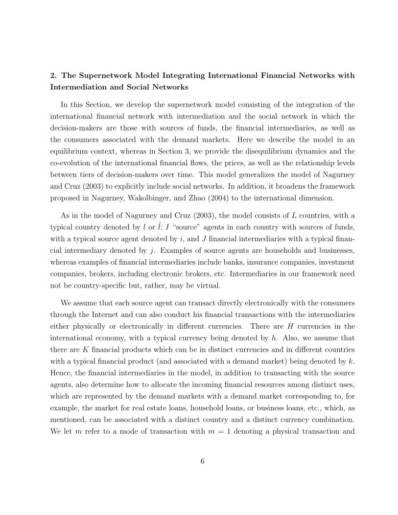
2. The Supernetwork Model Integrating International Financial Networks with

Intermediation and Social Networks

In this Section, we develop the supernetwork model consisting of the integration of the

international financial network with intermediation and the social network in which the

decision-makers are those with sources of funds, the financial intermediaries, as well as

the consumers associated with the demand markets. Here we describe the model in an

equilibrium context, whereas in Section 3, we provide the disequilibrium dynamics and the

co-evolution of the international financial flows, the prices, as well as the relationship levels

between tiers of decision-makers over time. This model generalizes the model of Nagurney

and Cruz (2003) to explicitly include social networks. In addition, it broadens the framework

proposed in Nagurney, Wakolbinger, and Zhao (2004) to the international dimension.

As in the model of Nagurney and Cruz (2003), the model consists of L countries, with a

typical country denoted by l or l; I “source” agents in each country with sources of funds,

with a typical source agent denoted by i, and J financial intermediaries with a typical finan-

cial intermediary denoted by j. Examples of source agents are households and businesses,

whereas examples of financial intermediaries include banks, insurance companies, investment

companies, brokers, including electronic brokers, etc. Intermediaries in our framework need

not be country-specific but, rather, may be virtual.

We assume that each source agent can transact directly electronically with the consumers

through the Internet and can also conduct his financial transactions with the intermediaries

either physically or electronically in different currencies. There are H currencies in the

international economy, with a typical currency being denoted by h. Also, we assume that

there are K financial products which can be in distinct currencies and in different countries

with a typical financial product (and associated with a demand market) being denoted by k.

Hence, the financial intermediaries in the model, in addition to transacting with the source

agents, also determine how to allocate the incoming financial resources among distinct uses,

which are represented by the demand markets with a demand market corresponding to, for

example, the market for real estate loans, household loans, or business loans, etc., which, as

mentioned, can be associated with a distinct country and a distinct currency combination.

We let m refer to a mode of transaction with m = 1 denoting a physical transaction and

6

Social Network

m1 m· · · j · · · mJ

Flows areRelationship Levelsm11 · · · mil · · · mIL

m111 m· · · khl · · · mKHL

?

@@

@@R

HHHHHHHHj

��

�� ?

@@

@@R

�����������)

���������

��

��

?

@@

@@R

PPPPPPPPPPPq

��

�� ?

HHHHHHHHj

���������

��

��

@@

@@R

· · · · · · · · ·

?

'

&

$

%The Supernetwork

International Financial Networkwith Intermediation

m1 m· · · j · · · mJ mJ+1

Flows areFinancial Transactionsm11 m· · · il · · · mIL

m111 m· · · khl · · · mKHL

· · · · · · · · ·

??

��

��

���������

@@

@@R?

��

��

PPPPPPPPPPPq

HHHHHHHHj

@@

@@R

?

��

��

�����������)

@@

@@R?

���������

HHHHHHHHj

@@

@@R

��

��

PPPPPPPPPPPq

HHHHHHHHj?

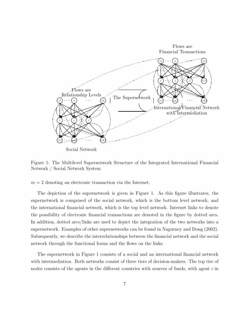
Figure 1: The Multilevel Supernetwork Structure of the Integrated International FinancialNetwork / Social Network System

m = 2 denoting an electronic transaction via the Internet.

The depiction of the supernetwork is given in Figure 1. As this figure illustrates, the

supernetwork is comprised of the social network, which is the bottom level network, and

the international financial network, which is the top level network. Internet links to denote

the possibility of electronic financial transactions are denoted in the figure by dotted arcs.

In addition, dotted arcs/links are used to depict the integration of the two networks into a

supernetwork. Examples of other supernetworks can be found in Nagurney and Dong (2002).

Subsequently, we describe the interrelationships between the financial network and the social

network through the functional forms and the flows on the links.

The supernetwork in Figure 1 consists of a social and an international financial network

with intermediation. Both networks consist of three tiers of decision-makers. The top tier of

nodes consists of the agents in the different countries with sources of funds, with agent i in

7

country l being referred to as agent il and associated with node il. There are, hence, IL top-

tiered nodes in the network. The middle tier of nodes in each of the two networks consists

of the intermediaries (which need not be country-specific), with a typical intermediary j

associated with node j in this (second) tier of nodes in the networks. The bottom tier of

nodes in both the social network and in the financial network consists of the demand markets,

with a typical demand market for product k in currency h and country l associated with node

khl. There are, as depicted in Figure 1, J middle (or second) tiered nodes corresponding to

the intermediaries and KHL bottom (or third) tiered nodes in the international financial

network. In addition, we add a node J +1 to the middle tier of nodes in the financial network

only in order to represent the possible non-investment (of a portion or all of the funds) by

one or more of the source agents (see also Nagurney and Ke (2003)).

The supernetwork in Figure 1 includes classical physical links as well as Internet links

to allow for electronic financial transactions. Electronic transactions are possible between

the source agents and the intermediaries, the source agents and the demand markets as well

as the intermediaries and the demand markets. Physical transactions can occur between

the source agents and the intermediaries and between the intermediaries and the demand

markets.

We now turn to the description of the behavior of the various economic decision-makers,

i.e., the source agents, the financial intermediaries, and the demand markets.

The Behavior of the Agents with Sources of Funds and their Optimality Condi-

tions

As described in Nagurney and Cruz (2003), we assume that each agent i in country l has

an amount of funds Sil available in the base currency. Since there are assumed to be H

currencies and 2 modes of transaction (physical or electronic), there are 2H links joining each

top tier node il with each middle tier node j; j = 1, . . . , J , with the first H links representing

physical transactions between a source and intermediary, and with the corresponding flow on

such a link given, respectively, by xiljh1, and the subsequent H links representing electronic

transactions with the corresponding flow given, respectively, by xiljh2. Hence, xil

jh1 denotes the

nonnegative amount invested (across all financial instruments) by source agent i in country

8

l in currency h transacted through intermediary j using the physical mode whereas xiljh2

denotes the analogue but for an electronic transaction. We group the financial flows for

all source agents/countries/intermediaries/currencies/modes into the column vector x1 ∈R2ILJH

+ . In addition, a source agent i in country l may transact directly with the consumers

at demand market k in currency h and country l via an Internet link. The nonnegative flow

on such a link joining node il with node khl is denoted by xilkhl

. We group all such financial

flows, in turn, into the column vector x2 ∈ RILKHL+ . Also, we let xil denote the (2JH+KHL)-

dimensional column vector associated with source agent il with components:{xiljhm, xil

khl; j =

1, . . . , J ; h = 1, . . . , H; m = 1, 2; k = 1, . . . , K; l = 1, . . . , L}. Furthermore, we construct a

link from each top tiered node to the second tiered node J +1 and associate a flow sil on such

a link emanating from node il to represent the possible nonnegative amount not invested by

agent i in country l.

For each source agent il the amount of funds transacted either electronically and/or

physically cannot exceed his financial holdings. Hence, the following conservation of flow

equation must hold:

J∑

j=1

H∑

h=1

2∑

m=1

xiljhm +

K∑

k=1

H∑

h=1

L∑

l=1

xilkhl

≤ Sil, ∀i, l. (1)

In Figure 1 the slack associated with constraint (1) for source agent i in country l is

represented as the flow on the link joining node il with the non-investment node J + 1.

Furthermore, let ηiljhm denote the nonnegative level of the relationship between source

agent il and intermediary j associated with currency h and mode of transaction m and let

ηilkhl

denote the nonnegative relationship level associated with the virtual mode of transaction

between source agent il and “demand market” khl. Each source agent il may actively

try to achieve a certain relationship level with an intermediary and/or a demand market.

We group the ηiljhms for all source agent/country/intermediary/currency/mode combinations

into the column vector η1 ∈ R2ILJH+ and the ηil

khls for all the source agent/country/demand

market/currency/country combinations into the column vector η2 ∈ RILKHL+ . Moreover,

we assume that these relationship levels take on a value that lies in the range [0, 1]. No

relationship is indicated by a relationship level of zero and the strongest possible relationship

is indicated by a relationship level of one. In the supernetwork depicted in Figure 1 the

9

relationship flows are associated with the links in the social network component of the

supernetwork. Specifically, the vector of flows η1 corresponds to flows on the links between

the source agents in the countries and the intermediaries, whereas the vector of flows η2

corresponds to the flows on the links between the source agents and the demand markets

in the various currencies and countries on the social network. The relationship levels, along

with the financial flows, are endogenously determined in the model.

The source agent may spend money, for example, in the form of gifts and/or additional

time/service in order to achieve a particular relationship level. The production cost functions

for relationship levels are denoted by biljhm and bil

khland represent, respectively, how much

money a source agent il has to spend in order to achieve a certain relationship level with

intermediary j transacting through mode m and currency h or in order to achieve a certain

relationship level with demand market khl. These relationship production cost functions

are distinct for each such combination. Their specific functional forms may be influenced by

such factors as the willingness of intermediaries or demand markets to establish/maintain a

relationship and the level of previous business relationships and private relationships that ex-

ist. In an international setting, in particular, cultural differences, difficulties with languages,

and distances, may also play a role in making it more costly to establish (and maintain) a

relationship level.

The relationship production cost function is assumed, hence, to be a function of the

relationship level between the source agent il and intermediary j transacting via mode m

and currency h or with the consumers at demand market khl, that is,

biljhm = bil

jhm(ηiljhm), ∀i, l, j, h, m, (2)

bilkhl

= bilkhl

(ηilkhl

), ∀i, l, k, h, l. (3)

We assume that these functions are convex and continuously differentiable.

We denote the transaction cost associated with source agent il transacting with interme-

diary j in currency h via mode m by ciljhm (and measured in the base currency) and assume

that:

ciljhm = cil

jhm(xiljhm, ηil

jhm), ∀i, l, j, h, m, (4)

10

that is, the cost associated with source agent i in country l transacting with intermediary

j in currency h depends on the volume of financial transactions between the particular pair

via the particular mode and on the relationship level between them. If the relationship level

increases, the transaction cost may be expected to decrease since higher relationship levels

may lead to higher levels of trust which can affect transactions. This is especially important

in international exchanges in which transaction costs may be significant.

We denote the transaction cost associated with source agent il transacting with demand

market k in country l in currency h via the Internet link by cilkhl

(and also measured in the

base currency) and assume that:

cilkhl

= cilkhl

(xilkhl

, ηilkhl

), ∀i, l, k, h, l, (5)

that is, the cost associated with source agent i in country l transacting with the consumers

for financial product k in currency h and country l. The transaction cost functions are

assumed to be convex and continuously differentiable and depend on the volume of flow of

the transaction and on the relationship level.

The source agent il faces total costs that equal the sum of the total transaction costs plus

the costs that he incurs for establishing relationship levels. His revenue, in turn, is equal

to the sum of the price (rate of return plus the rate of appreciation) that the agent can

obtain times the total quantity obtained/purchased. Let now ρil∗1jhm denote the actual price

charged agent il for the instrument in currency h by intermediary j transacting via mode

m and let ρil∗1khl

, in turn, denote the actual price associated with source agent il transacting

electronically with demand market khl. Let e∗h denote the actual rate of appreciation of

currency h against the base currency, which can be interpreted as the rate of return earned

due to exchange rate fluctuations (see Nagurney and Siokos (1997)). These “exchange” rates

are grouped into the column vector e∗ ∈ RH+ . We later discuss how such prices are recovered.

We assume that each source agent in each country seeks to maximize his net return with

the net revenue maximization problem for source agent il being given by:

MaximizeJ∑

j=1

H∑

h=1

2∑

m=1

(ρil∗1jhm+e∗h)x

iljhm+

K∑

k=1

H∑

h=1

L∑

l=1

(ρil∗1khl+e∗h)x

ilkhl

−J∑

j=1

H∑

h=1

2∑

m=1

ciljhm(xil

jhm, ηiljhm)

11

−K∑

k=1

H∑

h=1

L∑

l=1

cilkhl

(xilkhl

, ηilkhl

) −J∑

j=1

H∑

h=1

2∑

m=1

biljhm(ηil

jhm) −K∑

k=1

H∑

h=1

L∑

l=1

bilkhl

(ηilkhl

) (6)

subject to:

xiljhm ≥ 0, xil

khl≥ 0, ∀j, h, m, k, l, (7)

0 ≤ ηiljhm ≤ 1, 0 ≤ ηil

khl≤ 1, ∀j, h, m, k, l, (8)

and the constraint (1) for source agent il.

The first two terms in (6) represent the revenue. The next four terms represent the

various costs. The constraints are comprised of the conservation of flow equation (1), the

nonnegativity assumptions on the financial flows (cf. (7)) and on the relationship levels with

the latter being bounded from above by the value one (cf. (8)).

Furthermore, it is reasonable to assume that each source agent tries to minimize risk and

has been noted in empirical studies by Kim (1999). Here, for the sake of generality, and as

in the papers by Nagurney and Cruz (2003, 2004) and Nagurney, Wakolbinger, and Zhao

(2004), we assume, as given, a risk function for source agent il, dealing with intermediary

j via mode m and currency h, denoted by riljhm, and a risk function for source agent il

dealing with demand market khl denoted by rilkhl

. These functions depend not only on the

quantity of the financial flow transacted between the pair of nodes (and via a particular

currency and mode) but also on the corresponding relationship level. If the relationship

level increases, the risk is likely to decrease because trust reduces transaction uncertainty.

Since international financial transactions are potentially riskier, high relationship levels can

be of utmost significance and can, hence, create competitive advantages.

These risk functions are assumed to be as follows:

riljhm = ril

jhm(xiljhm, ηil

jhm), ∀i, l, j, h, m, (9)

rilkhl

= rilkhl

(xilkhl

, ηilkhl

), ∀i, l, k, h, l, (10)

where riljhm and ril

khlare assumed to be convex and continuously differentiable.

Hence, source agent il also faces an optimization problem associated with his desire to

12

minimize the total risk and corresponding to:

MinimizeJ∑

j=1

H∑

h=1

2∑

m=1

riljhm(xil

jhm, ηiljhm) +

K∑

k=1

H∑

h=1

L∑

l=1

rilkhl

(xilkhl

, ηilkhl

) (11)

subject to:

xiljhm ≥ 0, xil

khl≥ 0, ∀j, h, m, k, l, (12)

0 ≤ ηiljhm ≤ 1, 0 ≤ ηil

khl≤ 1, ∀j, h, m, k, l. (13)

In addition, the source agent also tries to maximize the relationship value generated by

interacting with other decision-makers in the network. Here, viljhm denotes the relationship

value function for source agent il, intermediary j, mode m and currency h, and viljhm is

assumed to be a function of the relationship level of il with intermediary j transacting via

mode m and currency h . Similarly, vilkhl

denotes the relationship value function for source

agent il and demand market khl. It is assumed to be a function of the relationship level

with the particular demand market khl such that

viljhm = vil

jhm(ηiljhm), ∀i, l, j, h, m, (14)

vilkhl

= vilkhl

(ηilkhl

), ∀i, l, k, h, l. (15)

We assume that the value functions are continuously differentiable and concave.

Hence, source agent il is also faced with the optimization problem representing the max-

imization of the total value of his relationships expressed mathematically as:

MaximizeJ∑

j=1

H∑

h=1

2∑

m=1

viljhm(ηil

jhm) +K∑

k=1

H∑

h=1

L∑

l=1

vilkhl

(ηilkhl

) (16)

subject to:

0 ≤ ηiljhm ≤ 1, 0 ≤ ηil

khl≤ 1, ∀j, h, m, k, l. (17)

The Multicriteria Decision-Making Problem Faced by a Source Agent

We can now construct the multicriteria decision-making problem facing a source agent which

allows him to weight the criteria of net revenue maximization (cf. (6)), risk minimization

13

(cf. (11)), and total relationship value maximization (see (16)) in an individual manner.

Source agent ils multicriteria decision-making objective function is denoted by U il. Assume

that source agent il assigns a nonnegative weight αil to the risk generated and a nonnegative

weight βil to the relationship value. The weight associated with net revenue maximization

serves as the numeraire and is set equal to 1. The nonnegative weights measure the im-

portance of risk and the total relationship value and, in addition, transform these values

into monetary units. We can now construct a value function for each source agent (cf.

Keeney and Raiffa (1993), Dong, Zhang, and Nagurney (2002), Nagurney, Wakolbinger, and

Zhao (2004), and the references therein) using a constant additive weight value function.

Therefore, the multicriteria decision-making problem of source agent il can be expressed as:

Maximize U il =J∑

j=1

H∑

h=1

2∑

m=1

(ρil∗1jhm + e∗h)x

iljhm +

K∑

k=1

H∑

h=1

L∑

l=1

(ρil∗1khl + e∗h)x

ilkhl

−J∑

j=1

H∑

h=1

2∑

m=1

ciljhm(xil

jhm, ηiljhm) −

K∑

k=1

H∑

h=1

L∑

l=1

cilkhl

(xilkhl

, ηilkhl

) −J∑

j=1

H∑

h=1

2∑

m=1

biljhm(ηil

jhm)

−K∑

k=1

H∑

h=1

L∑

l=1

bilkhl

(ηilkhl

) − αil(J∑

j=1

H∑

h=1

2∑

m=1

riljhm(xil

jhm, ηiljhm) +

K∑

k=1

H∑

h=1

L∑

l=1

rilkhl

(xilkhl

, ηilkhl

))

+βil(J∑

j=1

H∑

h=1

2∑

m=1

viljhm(ηil

jhm) +K∑

k=1

H∑

h=1

L∑

l=1

vilkhl

(ηilkhl

)) (18)

subject to:

xiljhm ≥ 0, xil

khl≥ 0, ∀j, h, m, k, l, (19)

0 ≤ ηiljhm ≤ 1, 0 ≤ ηil

khl≤ 1, ∀j, h, m, k, l, (20)

and the constraint (1) for source agent il.

The first six terms on the right-hand side of the equal sign in (18) represent the net revenue

which is to be maximized, the next two terms represent the weighted total risk which is to

be minimized and the last two terms represent the weighted total relationship value, which

is to be maximized. We can observe that such an objective function is in concert with those

used in classical portfolio optimization (see Markowitz (1952, 1959)) but substantially more

general to reflect specifically the additional criteria, notably, that of total relationship value

maximization.

14

Under the above assumed and imposed assumptions on the underlying functions, the

optimality conditions for all source agents simultaneously can be expressed as the following

inequality (cf. Bazaraa, Sherali, and Shetty (1993), Gabay and Moulin (1980); see also

Nagurney (1999)): determine (x1∗, x2∗, η1∗, η2∗) ∈ K1, satisfying

I∑

i=1

L∑

l=1

J∑

j=1

H∑

h=1

2∑

m=1

[αil ∂ril

jhm(xil∗jhm, ηil∗

jhm)

∂xiljhm

+∂cil

jhm(xil∗jhm, ηil∗

jhm)

∂xiljhm

− ρil∗1jhm − e∗h

]×

[xil

jhm − xil∗jhm

]

+I∑

i=1

L∑

l=1

J∑

j=1

H∑

h=1

L∑

l=1

[αil

∂rilkhl

(xil∗khl

, ηil∗khl

)

∂xilkhl

+∂cil

khl(xil∗

khl, ηil∗

khl)

∂xilkhl

− ρil∗1khl

− e∗h

]×

[xil

khl− xil∗

khl

]

+I∑

i=1

L∑

l=1

J∑

j=1

H∑

h=1

2∑

m=1

[∂cil

jhm(xil∗jhm, ηil∗

jhm)

∂ηiljhm

+∂bil

jhm(ηil∗jhm)

∂ηiljhm

− βil ∂viljhm(ηil∗

jhm)

∂ηiljhm

+αil ∂riljhm(xil∗

jhm, ηil∗jhm)

∂ηiljhm

]×

[ηil

jhm − ηil∗jhm

]

+I∑

i=1

L∑

l=1

K∑

k=1

H∑

h=1

L∑

l=1

[∂cil

khl(xil∗

khl, ηil∗

khl)

∂ηilkhl

+∂bil

khl(ηil∗

khl)

∂ηilkhl

− βil∂vil

khl(ηil∗

khl)

∂ηilkhl

+ αil∂ril

khl(xil∗

khl, ηil∗

khl)

∂ηilkhl

]

×[ηil

khl− ηil∗

khl

]≥ 0, ∀(x1, x2, η1, η2) ∈ K1, (21)

where

K1 ≡[(x1, x2, η1, η2)|xil

jhm ≥ 0, xilkhl

≥ 0, 0 ≤ ηiljhm ≤ 1, 0 ≤ ηil

khl≤ 1,

∀i, l, j, h, m, k, l, and (1) holds]

(22)

Inequality (21) is actually a variational inequality (cf. Nagurney (1999) and the references

therein).

The Behavior of the Intermediaries and their Optimality Conditions

The intermediaries (cf. Figure 1), in turn, are involved in transactions both with the source

agents in the different countries, as well as with the users of the funds, that is, with the

ultimate consumers associated with the markets for the distinct types of loans/products in

different currencies and countries and represented by the bottom tier of nodes of the network.

Each intermediary node j; j = 1, . . . , J , may transact with a demand market via a physical

link, and/or electronically via an Internet link. Hence, from each intermediary node j, we

15

construct two links to each node khl, with the first such link denoting a physical transaction

and the second such link – an electronic transaction. The corresponding flow, in turn, which

is nonnegative, is denoted by yj

khlm; m = 1, 2, and corresponds to the amount of the financial

product k in currency h and country l transacted from intermediary j via mode m. We

group the financial flows between node j and the bottom tier nodes into the column vector

yj ∈ R2KHL+ . All such financial flows for all the intermediaries are then further grouped into

the column vector y ∈ R2JKHL+ .

As in the case of source agents, the intermediaries have to bear some costs to establish

and maintain relationship levels with source agents and with the consumers. We denote the

relationship level between intermediary j and demand market khl transacting through mode

m by ηj

khlm. We group the relationship levels for all intermediary/demand market pairs into

the column vector η3 ∈ R2JKHL+ . We assume that the relationship levels are nonnegative

and that they may assume a value from 0 through 1. These relationship levels represent the

flows between the intermediaries and the demand market nodes in the social network level

of the supernetwork in Figure 1.

Let biljhm denote the cost function associated with the relationship between intermediary

j and source agent il transacting in currency h and via mode m and let bj

khlmdenote the

analogous cost function but associated with intermediary j, demand market khl, and mode

m. Note that these functions are from the perspective of the intermediary (whereas (2) and

(3) are from the perspective of the source agents). These cost functions are a function of the

relationship levels (as in the case of the source agents) and are given by:

biljhm = bil

jhm(ηiljhm), ∀i, l, j, h, m, (23)

bj

khlm= bj

khlm(ηj

khlm), ∀i, l, k, h, l, m. (24)

The intermediaries also have associated transaction costs in regards to transacting with

the source agents, which can depend on the type of currency as well as the source agent. We

denote the transaction cost associated with intermediary j transacting with source agent il

associated with currency h via mode m by ciljhm and we assume that it is of the form

ciljhm = cil

jhm(xiljhm, ηil

jhm), ∀i, l, j, h, m, (25)

16

that is, such a transaction cost is allowed to depend on the amount allocated by the particular

agent in a currency and transacted with the particular intermediary via the particular mode

as well as the relationship level between them. In addition, we assume that an intermediary

j also incurs a transaction cost cj

khlmassociated with transacting with demand market khl

through mode m, where

cj

khlm= cj

khlm(yj

khlm, ηj

khlm), ∀j, k, h, l, m. (26)

Hence, the transaction costs given in (26) can vary according to the intermediary/product/

currency/country/mode combination and are a function of the volume of the product trans-

acted and the relationship level.

In addition, an intermediary j is faced with what we term a handling/conversion cost,

which may include, for example, the cost of converting the incoming financial flows into the

financial loans/products associated with the demand markets. We denote such a cost faced

by intermediary j by cj and, in the simplest case, cj would be a function of∑I

i=1

∑Ll=1

∑Hh=1∑2

m=1 xiljhm, that is, the holding/conversion cost of an intermediary is a function of how much

he has obtained in the different currencies from the various source agents in the different

countries. For the sake of generality, however, we allow the function to depend also on the

amounts held by other intermediaries and, therefore, we may write:

cj = cj(x1), ∀j. (27)

We assume that the cost functions (23) – (27) are convex and continuously differentiable

and that the costs are measured in the base currency.

The actual price charged for the financial product k associated with intermediary j trans-

acting with the consumers in currency h via mode m and country l is denoted by ρj∗2khlm

,

for intermediary j. Similarly, as in the case of source agents, e∗h denote the actual rate of

appreciation in currency h. Later, we discuss how such prices are arrived at.

We assume that each intermediary seeks to maximize his net revenue with the net revenue

criterion for intermediary j being given by:

MaximizeK∑

k=1

H∑

h=1

L∑

l=1

2∑

m=1

(ρj∗2khlm

+ e∗h)yj

khlm− cj(x

1) −I∑

i=1

L∑

l=1

H∑

h=1

2∑

m=1

ciljhm(xil

jhm, ηiljhm)

17

−K∑

k=1

H∑

h=1

L∑

l=1

2∑

m=1

cj

khlm(yj

khlm, ηj

khlm) −

I∑

i=1

L∑

l=1

H∑

h=1

2∑

m=1

biljhm(ηil

jhm)

−K∑

k=1

H∑

h=1

L∑

l=1

2∑

m=1

bj

khlm(ηj

khlm) −

I∑

i=1

L∑

l=1

H∑

h=1

2∑

m=1

(ρil∗1jhm + e∗h)x

iljhm (28)

subject to:K∑

k=1

H∑

h=1

L∑

l=1

2∑

m=1

yj

khlm≤

I∑

i=1

L∑

l=1

H∑

h=1

2∑

m=1

xiljhm (29)

xiljhm ≥ 0, yj

khlm≥ 0, ∀i, l, h, l, m. (30)

0 ≤ ηiljhm ≤ 1, 0 ≤ ηj

khlm≤ 1, ∀i, l, h, m, k, l. (31)

Constraint (29) guarantees that each intermediary does not reallocate more financial

flows than he has available. Constraints (30) and (31) guarantee that the financial flows and

relationship levels are nonnegative (from the perspective of the intermediary) and that the

levels of the relationships do not exceed one.

In addition, we assume that each intermediary is also concerned with risk minimization.

For the sake of generality, we assume, as given, a risk function riljhm, for intermediary j in

transacting with source agent il in currency h through mode m and a risk function rj

khlmfor

intermediary j associated with his transacting with consumers at demand market khl through

mode m. The risk functions are assumed to be continuous and convex and a function of the

amount transacted with the particular source agent or demand market and the relationship

level with this source agent or demand market. A higher relationship level can be expected

to reduce risk since trust reduces transactional uncertainty. The risk functions may be dis-

tinct for each source agent/country/intermediary/currency/mode and intermediary/demand

market/currency/country/mode combination and are given, respectively, by:

riljhm = ril

jhm(xiljhm, ηil

jhm), ∀i, l, j, h, m, (32)

rj

khlm= rj

khlm(yj

khlm, ηj

khlm), ∀j, k, h, l, m. (33)

Since a financial intermediary j is assumed to minimize his total risk, he is also faced with

the optimization problem given by:

MinimizeI∑

i=1

L∑

l=1

H∑

h=1

2∑

m=1

riljhm(xil

jhm, ηiljhm) +

K∑

k=1

H∑

h=1

L∑

l=1

2∑

m=1

rj

khlm(yj

khlm, ηj

khlm) (34)

18

subject to:

xiljhm ≥ 0, yj

khlm≥ 0, ∀i, l, h, m, k, l, (35)

0 ≤ ηiljhm ≤ 1, 0 ≤ ηj

khlm≤ 1, ∀i, l, h, m, k, l. (36)

As in the case of the source agents, intermediary j also tries to maximize his relationship

values associated with the source agents and with the demand markets. We assume, as

given, a relationship value function viljhm for intermediary j in dealing with source agent

il in currency h through transaction mode m and a relationship value function vj

khlmfor

intermediary j associated with his transacting with consumers at demand market khl through

mode m. The relationship value functions are assumed to be continuously differentiable and

concave. They are assumed to be functions of the corresponding relationship levels and

given, respectively, by

viljhm = vil

jhm(ηiljhm), ∀i, l, j, h, m, (37)

vj

khlm= vj

khlm(ηj

khlm), ∀j, k, h, l, m. (38)

Finally, financial intermediary j tries to maximize his total relationship value, given

mathematically by the optimization problem:

MaximizeI∑

i=1

L∑

l=1

H∑

h=1

2∑

m=1

viljhm(ηil

jhm) +K∑

k=1

H∑

h=1

L∑

l=1

2∑

m=1

vj

khlm(ηj

khlm) (39)

subject to:

0 ≤ ηiljhm ≤ 1, 0 ≤ ηj

khlm≤ 1, ∀i, l, j, h, m, k, l. (40)

The Multicriteria Decision-Making Problem Faced by a Financial Intermediary

We are now ready to construct the multicriteria decision-making problem faced by an in-

termediary which combines with appropriate individual weights the criteria of net revenue

maximization given by (28); risk minimization, given by (34), and total relationship value

maximization, given by (39). In particular, we let intermediary j assign a nonnegative weight

δj to the total risk and a nonnegative weight γj to the total relationship value. The weight

associated with net revenue maximization is set equal to 1 and serves as the numeraire (as in

19

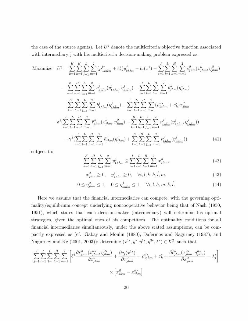
the case of the source agents). Let U j denote the multicriteria objective function associated

with intermediary j with his multicriteria decision-making problem expressed as:

Maximize U j =K∑

k=1

H∑

h=1

L∑

l=1

2∑

m=1

(ρj∗2khlm

+ e∗h)yj

khlm− cj(x

1) −I∑

i=1

L∑

l=1

H∑

h=1

2∑

m=1

ciljhm(xil

jhm, ηiljhm)

−K∑

k=1

H∑

h=1

L∑

l=1

2∑

m=1

cj

khlm(yj

khlm, ηj

khlm) −

I∑

i=1

L∑

l=1

H∑

h=1

2∑

m=1

biljhm(ηil

jhm)

−K∑

k=1

H∑

h=1

L∑

l=1

2∑

m=1

bj

khlm(ηj

khlm) −

I∑

i=1

L∑

l=1

H∑

h=1

2∑

m=1

(ρil∗1jhm + e∗h)x

iljhm

−δj(I∑

i=1

L∑

l=1

H∑

h=1

2∑

m=1

riljhm(xil

jhm, ηiljhm) +

K∑

k=1

H∑

h=1

L∑

l=1

2∑

m=1

rj

khlm(yj

khlm, ηj

khlm))

+γj(I∑

i=1

L∑

l=1

H∑

h=1

2∑

m=1

viljhm(ηil

jhm) +K∑

k=1

H∑

h=1

L∑

l=1

2∑

m=1

vj

khlm(ηj

khlm)) (41)

subject to:K∑

k=1

H∑

h=1

L∑

l=1

2∑

m=1

yj

khlm≤

I∑

i=1

L∑

l=1

H∑

h=1

2∑

m=1

xiljhm, (42)

xiljhm ≥ 0, yj

khlm≥ 0, ∀i, l, k, h, l, m, (43)

0 ≤ ηiljhm ≤ 1, 0 ≤ ηj

khlm≤ 1, ∀i, l, h, m, k, l. (44)

Here we assume that the financial intermediaries can compete, with the governing opti-

mality/equilibrium concept underlying noncooperative behavior being that of Nash (1950,

1951), which states that each decision-maker (intermediary) will determine his optimal

strategies, given the optimal ones of his competitors. The optimality conditions for all

financial intermediaries simultaneously, under the above stated assumptions, can be com-

pactly expressed as (cf. Gabay and Moulin (1980), Dafermos and Nagurney (1987), and

Nagurney and Ke (2001, 2003)): determine (x1∗, y∗, η1∗, η3∗, λ∗) ∈ K2, such that

J∑

j=1

I∑

i=1

L∑

l=

H∑

h=1

2∑

m=1

[δj ∂ril

jhm(xil∗jhm, ηil∗

jhm)

∂xiljhm

+∂cj(x

1∗)

∂xiljhm

+ ρil∗1jhm + e∗h +

∂ciljhm(xil∗

jhm, ηil∗jhm)

∂xiljhm

− λ∗j

]

×[xil

jhm − xil∗jhm

]

20

+J∑

j=1

K∑

k=1

H∑

h=1

L∑

l=1

2∑

m=1

δj

∂rj

khlm(yj∗

khlm, ηj∗

khlm)

∂yj

khlm

+∂cj

khlm(yj∗

khlm, ηj∗

khlm)

∂yj

khlm

− ρj∗2khlm

− e∗h + λ∗j

×[yj

khlm− yj∗

khlm

]

+J∑

j=1

I∑

i=1

L∑

l=

H∑

h=1

2∑

m=1

[δj ∂ril

jhm(xil∗jhm, ηil∗

jhm)

∂ηiljhm

+∂cil

jhm(xil∗jhm, ηil∗

jhm)

∂ηiljhm

− γj ∂viljhm(ηil∗

jhm)

∂ηiljhm

+∂bil

jhm(ηil∗jhm)

∂ηiljhm

×

[ηil

jhm − ηil∗jhm

]

+J∑

j=1

K∑

k=1

H∑

h=1

L∑

l=1

2∑

m=1

δj

∂rj

khlm(yj∗

khlm, ηj∗

khlm)

∂ηj

khlm

+∂cj

khlm(yj∗

khlm, ηj∗

khlm)

∂ηj

khlm

− γj∂vj

khlm(ηj∗

khlm)

∂ηj

khlm

+∂bj

khl(ηj∗khlm

)

∂ηj

khlm

×

[ηj

khlm− ηj∗

khlm

]

+J∑

j=1

I∑

i=1

L∑

l=1

H∑

h=1

2∑

m=1

xil∗jhm −

K∑

k=1

H∑

h=1

L∑

l=1

2∑

m=1

yj∗khlm

×

[λj − λ∗

j

]≥ 0, ∀(x1, y, η1, η3, λ) ∈ K2,

(45)

where

K2 ≡[(x1, y, η1, η3, λ)|xil

jhm ≥ 0, yj

khlm≥ 0, 0 ≤ ηil

jhm ≤ 1, 0 ≤ ηj

khlm≤ 1, λj ≥ 0,

∀i, l, j, h, m, k, l]. (46)

Here λj denotes the Lagrange multiplier associated with constraint (42) and λ is the

column vector of all the intermediaries’ Lagrange multipliers. These Lagrange multipliers

can also be interpreted as shadow prices. Indeed, according to the fifth term in (45), λ∗j

serves as the price to “clear the market” at intermediary j.

Inequality (45) provides us with conditions under which optimal virtual and/or physical

financial transactions between intermediaries and source agents occur and optimal condi-

tions under which virtual transactions between source agents and demand markets occur.

Furthermore, it formulates the optimality conditions under which the relationship levels as-

sociated with intermediaries interacting with either the source agents or the demand markets

will take on positive values; in other words, a relationship exists.

21

The Consumers at the Demand Markets and the Equilibrium Conditions

We now describe the consumers located at the demand markets. The consumers take into

account in making their consumption decisions not only the price charged for the financial

product by the agents with source of funds and intermediaries but also their transaction

costs associated with obtaining the product.

Let cj

khlmdenote the transaction cost associated with obtaining product k in currency

h in country l via mode m from intermediary j and recall that yj

khlmis the amount of the

financial product k in currency h flowing between intermediary j and consumers in country

l via mode m. We assume that the transaction cost is measured in the base currency, is

continuous, and of the general form:

cj

khlm= cj

khlm(x2, y, η2, η3), ∀j, k, h, l, m. (47)

Hence, the cost of transacting between an intermediary and a demand market via a specific

mode, from the perspective of the consumers, can depend upon the volume of financial flows

transacted either physically and/or electronically from intermediaries as well as from source

agents and the associated relationship levels. As in the case of the source agents and the

financial intermediaries, higher relationship levels potentially reduce transaction costs, which

means that they can lead to quantifiable cost reductions. The generality of this cost function

structure enables the modeling of competition on the demand side. Moreover, it allows for

information exchange between the consumers at the demand markets who may inform one

another as to their relationship levels which, in turn, can affect the transaction costs.

In addition, let cilkhl

denote the transaction cost associated with obtaining the financial

product k in currency h in country l electronically from source agent il, where we assume

that the transaction cost is continuous and of the general form:

cilkhl

= cilkhl

(x2, y, η2, η3), ∀i, l, k, h, l. (48)

Hence, the transaction cost associated with transacting directly with source agents is of

a form of the same level of generality as the transaction costs associated with transacting

with the financial intermediaries.

22

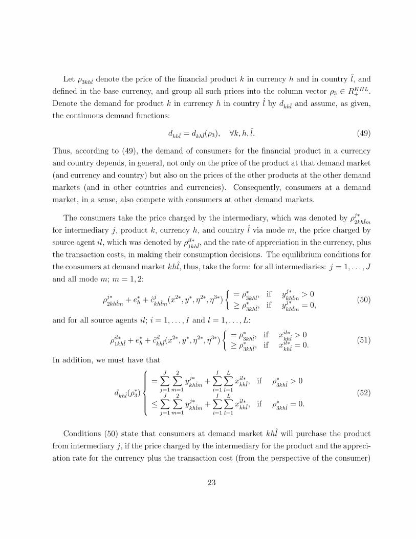
Let ρ3khl denote the price of the financial product k in currency h and in country l, and

defined in the base currency, and group all such prices into the column vector ρ3 ∈ RKHL+ .

Denote the demand for product k in currency h in country l by dkhl and assume, as given,

the continuous demand functions:

dkhl = dkhl(ρ3), ∀k, h, l. (49)

Thus, according to (49), the demand of consumers for the financial product in a currency

and country depends, in general, not only on the price of the product at that demand market

(and currency and country) but also on the prices of the other products at the other demand

markets (and in other countries and currencies). Consequently, consumers at a demand

market, in a sense, also compete with consumers at other demand markets.

The consumers take the price charged by the intermediary, which was denoted by ρj∗2khlm

for intermediary j, product k, currency h, and country l via mode m, the price charged by

source agent il, which was denoted by ρil∗1khl

, and the rate of appreciation in the currency, plus

the transaction costs, in making their consumption decisions. The equilibrium conditions for

the consumers at demand market khl, thus, take the form: for all intermediaries: j = 1, . . . , J

and all mode m; m = 1, 2:

ρj∗2khlm

+ e∗h + cj

khlm(x2∗, y∗, η2∗, η3∗)

{= ρ∗

3khl, if yj∗

khlm> 0

≥ ρ∗3khl

, if yj∗khlm

= 0,(50)

and for all source agents il; i = 1, . . . , I and l = 1, . . . , L:

ρil∗1khl

+ e∗h + cilkhl

(x2∗, y∗, η2∗, η3∗)

{= ρ∗

3khl, if xil∗

khl> 0

≥ ρ∗3khl

, if xil∗khl

= 0.(51)

In addition, we must have that

dkhl(ρ∗3)

=J∑

j=1

2∑

m=1

yj∗khlm

+I∑

i=1

L∑

l=1

xil∗khl

, if ρ∗3khl

> 0

≤J∑

j=1

2∑

m=1

yj∗khlm

+I∑

i=1

L∑

l=1

xil∗khl

, if ρ∗3khl

= 0.

(52)

Conditions (50) state that consumers at demand market khl will purchase the product

from intermediary j, if the price charged by the intermediary for the product and the appreci-

ation rate for the currency plus the transaction cost (from the perspective of the consumer)

23

does not exceed the price that the consumers are willing to pay for the product in that

currency and country, i.e., ρ∗3khl

. Note that, according to (50), if the transaction costs are

identically equal to zero, then the price faced by the consumers for a given product is the

price charged by the intermediary for the particular product and currency in the country

plus the rate of appreciation in the currency. Condition (51) state the analogue, but for the

case of electronic transactions with the source agents.

Condition (52), on the other hand, states that, if the price the consumers are willing to

pay for the financial product at a demand market is positive, then the quantity of at the

demand market is precisely equal to the demand.

In equilibrium, conditions (50), (51), and (52) will have to hold for all demand markets

and these, in turn, can be expressed also as an inequality analogous to those in (21) and

(45) and given by: determine (x2∗, y∗, ρ∗3) ∈ R

(IL+2J+1)KHL+ , such that

J∑

j=1

K∑

k=1

H∑

h=1

L∑

l=1

2∑

m=1

[ρj∗

2khlm+ e∗h + cj

khlm(x2∗, y∗, η2∗, η3∗) − ρ∗

3khl

]×

[yj

khlm− yj∗

khlm

]

+I∑

i=1

L∑

l=1

K∑

k=1

H∑

h=1

L∑

l=1

[ρil∗

1khl+ e∗h + cil

khl(x2∗, y∗, η2∗, η3∗) − ρ∗

3khl

]×

[xil

khl− xil∗

khl

]

+K∑

k=1

H∑

h=1

L∑

l=1

J∑

j=1

2∑

m=1

yj∗khlm

+I∑

i=1

L∑

l=1

xil∗khl

− dkhl(ρ∗3)

×

[ρ3khl − ρ∗

3khl

]≥ 0,

∀(x2, y, ρ3) ∈ R(IL+2J+1)KHL+ . (53)

For further background, see Nagurney and Dong (2002).

The Equilibrium Conditions of the Supernetwork Integrating the International

Financial Network and the Social Network

In equilibrium, the financial flows that the source agents in different countries transact with

the intermediaries must coincide with those that the intermediaries actually accept from

them. In addition, the amounts of the financial products that are obtained by the consumers

in the different countries and currencies must be equal to the amounts that both the source

agents and the intermediaries actually provide. Hence, although there may be competition

24

between decision-makers at the same level of tier of nodes of the financial network there must

be, in a sense, cooperation between decision-makers associated with pairs of nodes (through

positive flows on the links joining them). Thus, in equilibrium, the prices and financial

flows must satisfy the sum of the optimality conditions (21) and (45) and the equilibrium

conditions (53). We make these relationships rigorous through the subsequent definition and

variational inequality derivation below.

Definition 1: Supernetwork Integrating the International Financial Network and

the Social Network

The equilibrium state of the supernetwork integrating the international financial network with

the social network is one where the financial flows and relationship levels between the tiers of

the network coincide and the financial flows, relationship levels, and prices satisfy the sum

of conditions (21), (45), and (53).

The equilibrium state is equivalent to the following:

Theorem 1: Variational Inequality Formulation

The equilibrium conditions governing the supernetwork integrating the international financial

network with the social network according to Definition 1 are equivalent to the solution of the

variational inequality given by: determine (x1∗, x2∗, y∗, η1∗, η2∗, η3∗, λ∗, ρ∗3) ∈K, satisfying:

I∑

i=1

L∑

l=1

J∑

j=1

H∑

h=1

2∑

m=1

[αil ∂ril

jhm(xil∗jhm, ηil∗

jhm)

∂xiljhm

+∂cil

jhm(xil∗jhm, ηil∗

jhm)

∂xiljhm

+ δj ∂riljhm(xil∗

jhm, ηil∗jhm)

∂xiljhm

+∂cj(x

1∗)

∂xiljhm

+∂cil

jhm(xil∗jhm, ηil∗

jhm)

∂xiljhm

− λ∗j

]×

[xil

jhm − xil∗jhm

]

+I∑

i=1

L∑

l=1

K∑

k=1

H∑

h=1

L∑

l=1

[αil

∂rilkhl

(xil∗khl

, ηil∗khl

)

∂xilkhl

+∂cil

khl(xil∗

khl, ηil∗

khl)

∂xilkhl

+ cilkhl

(x2∗, y∗, η2∗, η3∗) − ρ∗3khl

]

×[xil

khl− xil∗

khl

]

+J∑

j=1

K∑

k=1

H∑

h=1

L∑

l=1

2∑

m=1

δj

∂rj

khlm(yj∗

khlm, ηj∗

khlm)

∂yj

khlm

+∂cj

khlm(yj∗

khlm, ηj∗

khlm)

∂yj

khlm

+ cj

khlm(x2∗, y∗, η2∗, η3∗)

25

+λ∗j − ρ∗

3khl

]×

[yj

khlm− yj∗

khlm

]

+I∑

i=1

L∑

l=1

J∑

j=1

H∑

h=1

2∑

m=1

[∂cil

jhm(xil∗jhm, ηil∗

jhm)

∂ηiljhm

+∂cil

jhm(xil∗jhm, ηil∗

jhm)

∂ηiljhm

− βil ∂viljhm(ηil∗

jhm)

∂ηiljhm

−γj ∂viljhm(ηil∗

jhm)

∂ηiljhm

+ αil ∂riljhm(xil∗

jhm, ηil∗jhm)

∂ηiljhm

+ δj ∂riljhm(xil∗

jhm, ηil∗jhm)

∂ηiljhm

+∂bil

jhm(ηil∗jhm)

∂ηiljhm

+∂bil

jhm(ηil∗jhm)

∂ηiljhm

×

[ηil

jhm − ηil∗jhm

]

+I∑

i=1

L∑

l=1

K∑

k=1

H∑

h=1

L∑

l=1

[∂cil

khl(xil∗

khl, ηil∗

khl)

∂ηilkhl

+∂bil

khl(ηil∗

khl)

∂ηilkhl

− βil∂vil

khl(ηil∗

khl)

∂ηilkhl

+ αil∂ril

khl(xil∗

khl, ηil∗

khl)

∂ηilkhl

]

×[ηil

khl− ηil∗

khl

]

+J∑

j=1

K∑

k=1

H∑

h=1

L∑

l=1

2∑

m=1

δj

∂rj

khlm(yj∗

khlm, ηj∗

khlm)

∂ηj

khlm

+∂cj

khlm(yj∗

khlm, ηj∗

khlm)

∂ηj

khlm

− γj∂vj

khlm(ηj∗

khlm)

∂ηj

khlm

+∂bj

khl(ηj∗khlm

)

∂ηj

khlm

×

[ηj

khlm− ηj∗

khlm

]

+J∑

j=1

I∑

i=1

L∑

l=1

H∑

h=1

2∑

m=1

xil∗jhm −

K∑

k=1

H∑

h=1

L∑

l=1

2∑

m=1

yj∗khlm

×

[λj − λ∗

j

]

+K∑

k=1

H∑

h=1

L∑

l=1

J∑

j=1

2∑

m=1

yj∗khlm

+I∑

i=1

L∑

l=1

xil∗khl

− dkhl(ρ∗3)

×

[ρ3khl − ρ∗

3khl

]≥ 0,

∀(x1, x2, y, η1, η2, η3, λ, ρ3) ∈ K, (54)

where

K ≡[(x1, x2, y, η1, η2, η3, λ, ρ3)|xil

jhm ≥ 0, xilkhl

≥ 0, yj

khlm≥ 0, 0 ≤ ηil

jhm ≤ 1, 0 ≤ ηilkhl

≤ 1,

0 ≤ ηj

khlm≤ 1, ρ3khl ≥ 0, λj ≥ 0, ∀i, l, j, h, m, k, l, and (1) holds

]. (55)

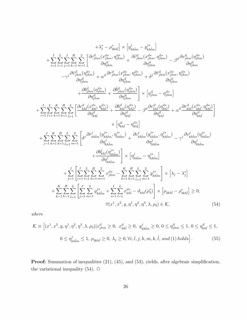
Proof: Summation of inequalities (21), (45), and (53), yields, after algebraic simplification,

the variational inequality (54). 2

26

We now put variational inequality (54) into standard form which will be utilized in the

subsequent sections. For additional background on variational inequalities and their appli-

cations, see the book by Nagurney (1999). In particular, we have that variational inequality

(54) can be expressed as:

〈F (X∗), X − X∗〉 ≥ 0, ∀X ∈ K, (56)

where X ≡ (x1, x2, y, η1, η2, η3, λ, ρ3) and F (X) ≡ (Filjhm, Filkhl, Fjkhlm, Filjhm, Filkhl, Fjkhlm,

Fj, Fkhl) with indices: i = 1, . . . , I; l = 1, . . . , L; j = 1, . . . , J ; h = 1, . . . , H; l = 1, . . . , L; m =

1, 2, and the specific components of F given by the functional terms preceding the multipli-

cation signs in (56), respectively. The term 〈·, ·〉 denotes the inner product in N -dimensional

Euclidean space.

We now describe how to recover the prices associated with the first two tiers of nodes in

the international financial network. Clearly, the components of the vector ρ∗3 are obtained

directly from the solution of variational inequality (56) as will be demonstrated explicitly

through several numerical examples in Section 5. In order to recover the second tier prices

associated with the intermediaries and the exchange rates one can (after solving variational

inequality (56) for the particular numerical problem) either (cf. (50)) set ρj∗2khlm

+ e∗h =[ρ∗

3khl− cj

khlm(x2∗, y∗, η2∗, η3∗)

], for any j, k, h, l, m such that yj∗

khlm> 0, or (cf. (45)) for any

yj∗khlm

> 0, set ρj∗2khlm

+ e∗h =[δj ∂rj

khlm(yj∗

khlm,ηj∗

khlm)

∂yj

khlm

+∂cj

khl(yj∗

khlm,ηj∗

khlm)

∂yj

khlm

+ λ∗j

].

Similarly, from (21) we can infer that the top tier prices comprising the vector ρ∗1 can

be recovered (once the variational inequality (56) is solved with particular data) thus: for

any i, l, j, h, m, such that xil∗jhm > 0, set ρil∗

1jhm + e∗h=[αil ∂ril

jhm(xil∗jhm,ηil∗

jhm)

∂xiljhm

+∂cil

jhm(xil∗jhm,ηil∗

jhm)

∂xiljhm

], or,

equivalently, (cf. (45)), to[λ∗

j − δj ∂riljhm(xil∗

jhm,ηil∗jhm)

∂xiljhm

− ∂cj(x1∗)

∂xiljhm

− ∂ciljhm(xil∗

jhm,ηil∗jhm)

∂xiljhm

].

In addition, in order to recover the first tier prices associated with the demand market

and the exchange rates one can (after solving variational inequality (56) for the particu-

lar numerical problem) either (cf. (21)) set ρil∗1khl

+ e∗h =[αil ∂ril

khl(xil∗

khl,ηil∗

khl)

∂xilkhl

+∂cil

khl(xil∗

khl,ηil∗

khl)

∂xilkhl

],

for any i, l, k, h, l such that xil∗khl

> 0, or (cf. (51)) for any xil∗khl

> 0, set ρil∗1khl

+ e∗h =[ρ∗

3khl− cil

khl(x2∗, y∗, η2∗, η3∗)

].

Under the above pricing mechanism, the optimality conditions (21) and (45) as well as

27

Social Network

η11∗111

m1 m· · · j · · · mJ ηIL∗KHL

Flows areRelationship Levelsm11 · · · mil · · · mIL

m111 m· · · khl · · · mKHL

?

@@

@@R

HHHHHHHHj

��

�� ?

@@

@@R

�����������)

���������

��

��

?

@@

@@R

PPPPPPPPPPPq

��

�� ?

HHHHHHHHj

���������

��

��

@@

@@R

· · · · · · · · ·

?

'

&

$

%The Supernetwork

International Financial Networkwith Intermediation

m1x11∗111

m· · · j · · · mJ mJ+1 xIL∗KHL

Flows areFinancial Transactions

m11 m· · · il · · · mIL

m111 m· · · khl · · · mKHL ρ∗3KHL

· · · · · · · · ·

??

��

��

���������

@@

@@R?

��

��

PPPPPPPPPPPq

HHHHHHHHj

@@

@@R

?

��

��

�����������)

@@

@@R?

���������

HHHHHHHHj

@@

@@R

��

��

PPPPPPPPPPPq

HHHHHHHHj?

Figure 2: The Supernetwork at Equilibrium

the equilibrium conditions (53) also hold separately (as well as for each individual decision-

maker).

In Figure 2, we display the supernetwork in equilibrium in which the equilibrium financial

flows, relationship levels, and prices now appear. Note that, if the equilibrium values of the

flows (be they financial or relationship levels) on links are identically equal to zero, then

those links can effectively be removed from the supernetwork (in equilibrium). Moreover,

the size of the equilibrium flows represent the “strength” of respective links (as discussed also

in the social network/supply chain network equilibrium model of Wakolbinger and Nagurney

(2004)). Thus, the supernetwork model developed here also provides us with the emergent

integrated social and financial network structures. In the next section, we discuss the dy-

namic evolution of the financial flows, relationship levels, and prices until this equilibrium is

achieved.

28

3. The Dynamic Adjustment Process

In this section, we describe the dynamics associated with the supernetwork model devel-

oped in Section 2 and formulate the corresponding dynamic model as a projected dynamical

system (cf. Nagurney and Zhang (1996a), Nagurney and Ke (2003), Nagurney and Cruz

(2004), and Nagurney, Wakolbinger, and Zhao (2004)). Importantly, the set of stationary

points of the projected dynamical system which formulates the dynamic adjustment process

will coincide with the set of solutions to the variational inequality problem (54). In par-

ticular, we describe the disequilibrium dynamics of the international financial flows, the

relationship levels, as well as the prices.

The Dynamics of the Financial Flows from the Source Agents

Note that, unlike the financial flows (as well as the prices associated with the distinct nodal

tiers of the network) between the intermediaries and the demand markets, the financial flows

from the source agents are subject not only to nonnegativity constraints but also to budget

constraints (cf. (1)). Hence, in order to guarantee that these constraints are not violated we

need to introduce some additional machinery based on projected dynamical systems theory

in order to describe the dynamics of these financial flows (see also, e.g., Nagurney and Siokos

(1997), Nagurney and Zhang (1996a), Nagurney and Cruz (2004), and Nagurney, Cruz, and

Matsypura (2003)).

In particular, we denote the rate of change of the vector of financial flows from source

agent il by xil and noting that the best realizable direction for the financial flows from source

agent il must include the constraints, we have that:

xil = ΠKil(xil,−F il), (57)

where ΠK is defined as (see also Nagurney and Zhang (1996a)):

ΠK(x, v) = limδ→0

PK(x + δv) − x

δ, (58)

and PK is the norm projection defined by

PK(x) = argminx′∈K‖x′ − x‖. (59)

29

The feasible set Kil is defined as: Kil ≡ {xil|xil ∈ R2JH+KHL+ and satisfies (1)}, and F il is the

vector (see following (56)) with components: Filjhm, Filkhl and with indices: j = 1, . . . , J ;

h = 1, . . . , H; m = 1, 2, and k = 1, . . . , K. Hence, expression (57) reflects that the financial

flow on a link emanating from a source agent will increase if the price (be it the market-

clearing price associated with an intermediary or a demand market price) exceeds the various

costs and weighted marginal risk; it will decrease if the latter exceeds the former.

The Dynamics of the Financial Products between the Intermediaries and the

Demand Markets

The rate of change of the financial flow yj

khlm, denoted by yj

khlm, is assumed to be equal to

the difference between the price the consumers are willing to pay for the financial product

at the demand market minus the price charged and the various transaction costs and the

weighted marginal risk associated with the transaction. Here we also guarantee that the

financial flows do not become negative. Hence, we may write: for every j, k, h, l, m:

yj

khlm=

ρ3khl − δj ∂rj

khlm(yj

khlm,ηj

khlm)

∂yj

khlm

− ∂cj

khlm(yj

khlm,ηj

khlm)

∂yj

khlm

−cj

khlm(x2, y, η2, η3) − λj, if yj

khlm> 0

max{0, ρ3khl − δj ∂rj

khlm(yj

khlm,ηj

khlm)

∂yj

khlm

− ∂cj

khlm(yj

khlm,ηj

khlm)

∂yj

khlm

−cj

khlm(x2, y, η2, η3) − λj}, if yj

khlm= 0.

(60)

Hence, according, to (60), if the price that the consumers are willing to pay for the product

(in the currency and country) exceeds the price that the intermediary charges and the various

transaction costs and weighted marginal risk, then the volume of flow of the product to that

demand market will increase; otherwise, it will decrease (or remain unchanged).

The Dynamics of the Relationship Levels between the Source Agents and the

Financial Intermediaries

Now the dynamics of the relationship levels between the source agents in the various countries

and the intermediaries are described. The rate of change of the relationship level ηiljhm,

denoted by ηiljhm, is assumed to be equal to the difference between the weighted relationship

value for source agent il, intermediary j, currency h and mode m, and the sum of the

30

marginal costs and the weighted marginal risks. Again, one must also guarantee that the

relationship levels do not become negative. Moreover, they may not exceed the level equal

to one. Hence, we can immediately write:

ηiljhm =

βil ∂viljhm(ηil

jhm)

∂ηiljhm

+ γj ∂viljhm(ηil

jhm)

∂ηiljhm

− ∂ciljhm(xil

jhm,ηiljhm)

∂ηiljhm

−∂ciljhm

(xiljhm

,ηiljhm

)

∂ηiljhm

− αil ∂riljhm

(xiljhm

,ηiljhm

)

∂ηiljhm

− δj ∂riljhm

(xiljhm

,ηiljhm

)

∂ηiljhm

−∂biljhm(ηil

jhm)

∂ηiljhm

− ∂biljhm(ηil∗

jhm)

∂ηiljhm

, if 0 < ηiljhm < 1

min{1, max{0, βil ∂viljhm(ηil

jhm)

∂ηiljhm

+ γj ∂viljhm(ηil

jhm)

∂ηiljhm

− ∂ciljhm(xil

jhm,ηiljhm)

∂ηiljhm

−∂ciljhm(xil

jhm,ηiljhm)

∂ηiljhm

− αil ∂riljhm(xil

jhm,ηiljhm)

∂ηiljhm

− δj ∂riljhm(xil

jhm,ηiljhm)

∂ηiljhm

−∂biljhm(ηil

jhm)

∂ηiljhm

− ∂biljhm(ηil

jhm)

∂ηiljhm

}}, otherwise,

(61)

where ηiljhm denotes the rate of change of the relationship level ηil

jhm.

This shows that if the sum of the weighted relationship values for the source agent and

the intermediary are higher than the total marginal costs plus the total weighted marginal

risk, then the level of relationship between that financial source agent and intermediary pair

will increase. If it is lower, the relationship value will decrease.

The Dynamics of the Relationship Levels between the Source Agents and the

Demand Markets

Here we describe the dynamics of the relationship levels between the source agents and the

demand markets. The rate of change of the relationship level ηilkhl

in turn, responds to the

difference between the weighted relationship value for source agent il and the sum of the

marginal costs and weighted marginal risks . One also must guarantee that these relationship

31

levels do not become negative (nor higher than one). Hence, one may write:

ηilkhl

=

βil ∂vilkhl

(ηilkhl

)

∂ηilkhl

− ∂cilkhl

(xilkhl

,ηilkhl

)

∂ηilkhl

− ∂bilkhl

(ηilkhl

)

∂ηilkhl

− αil ∂rilkhl

(xilkhl

,ηilkhl

)

∂ηilkhl

, if 0 < ηilkhl

< 1,

min{1, max{0, βil ∂vilkhl

(ηilkhl

)

∂ηilkhl

− ∂cilkhl

(xilkhl

,ηilkhl

)

∂ηilkhl

− ∂bilkhl

(ηilkhl

)

∂ηilkhl

−αil ∂rilkhl

(xilkhl

,ηilkhl

)

∂ηilkhl

}}, otherwise

(62)

where ηilkhl

denotes the rate of change of the relationship level ηilkhl

. This shows that if

the weighted relationship value for the source agent is higher than the total marginal costs

plus the total weighted marginal risk, then the level of relationship between that financial

source agent and demand market pair will increase. If it is lower, the relationship value will

decrease. Of course, the bounds on the relationship levels must also hold.

The Dynamics of the Relationship Levels between the Financial Intermediaries

and the Demand Markets

The dynamics of the relationship levels between the financial intermediaries and demand

markets are now described. The rate of change of the relationship level product ηj

khlmtrans-

acted via mode m is assumed to be equal to the difference between the weighted relationship

value for intermediary j and the sum of the marginal costs and weighted marginal risks,

where, of course, one also must guarantee that the relationship levels do not become nega-

tive nor exceed one. Hence, one may write:

ηj

khlm=

γj ∂vj

khlm(ηj

khlm)

∂ηj

khlm

− δj ∂rj

khlm(yj

khlm,ηj

khlm)

∂ηj

khlm

− ∂cj

khlm(yj

khlm,ηj

khlm)

∂ηj

khlm

−∂bjkhl

(ηj

khlm)

∂ηj

khlm

, if 0 < ηj

khlm< 1,

min{1, max{0, γj ∂vj

khlm(ηj∗

khlm)

∂ηj

khlm

− δj ∂rj

khlm(yj

khlm,ηj

khlm)

∂ηj

khlm

−∂cj

khlm(yj

khlm,ηj

khlm)

∂ηj

khlm

− ∂bjkhl

(ηj

khlm)

∂ηj

khlm

}}, otherwise,

(63)

where ηj

khlmdenotes the rate of change of the relationship level ηj

khlm. Expression (63)

reveals that if the weighted relationship value for the intermediary with the demand market

is higher than the total marginal costs plus the total weighted marginal risk, then the level of

32

relationship between that intermediary and demand market pair will increase. If it is lower,

the relationship value will decrease.

Demand Market Price Dynamics

We assume that the rate of change of the price ρ3khl, denoted by ρ3khl, is equal to the difference

between the demand for the financial product at the demand market in the currency and

country and the amount of the product actually available at that particular market. Hence, if

the demand for the product at the demand market at an instant in time exceeds the amount

available from the various intermediaries and source agents, then the price will increase; if the

amount available exceeds the demand at the price, then the price will decrease. Moreover, it

is guaranteed that the prices do not become negative. Thus, the dynamics of the price ρ3khl

for each k, h, l can be expressed as:

ρ3khl =

{dkhl(ρ3) −

∑Jj=1

∑2m=1 yj

khlm− ∑I

i=1

∑Ll=1 xil

khl, if ρ3khl > 0

max{0, dkhl(ρ3) −∑J

j=1

∑2m=1 yj

khlm− ∑I

i=1

∑Ll=1 xil

khl}, if ρ3khl = 0.

(64)

The Dynamics of the Prices at the Intermediaries

The prices at the intermediaries, whether they are physical or virtual, must reflect supply

and demand conditions as well. In particular, we let λj denote the rate of change in the

market clearing price associated with intermediary j and we propose the following dynamic

adjustment for every intermediary j:

λj =

{ ∑Kk=1

∑Hh=1

∑Ll=1

∑2m=1 yj

khlm− ∑I

i=1

∑Ll=1

∑Hh=1

∑2m=1 xil

jhm, if λj > 0

max{0, ∑Kk=1

∑Hh=1

∑Ll=1

∑2m=1 yj

khlm− ∑I

i=1

∑Ll=1

∑Hh=1

∑2m=1 xil

jhm}, if λj = 0.

(65)

Hence, if the financial flows from the source agents in the countries into an intermedi-

ary exceed the amount demanded at the demand markets from the intermediary, then the

market-clearing price at that intermediary will decrease; if, on the other hand, the volume

of financial flows into an intermediary is less than that demanded by the consumers at the

demand markets (and handled by the intermediary), then the market-clearing price at that

intermediary will increase.

33

The Projected Dynamical System

We now turn to stating the complete dynamic model. In the dynamic model the flows

evolve according to the mechanisms described above; specifically, the financial flows from

the source agents evolve according to (57) for all source agents il. The financial flows from

the financial intermediaries to the demand markets evolve according to (60) for all financial

intermediaries j, demand markets khl, and modes m. The relationship levels between source

agents and financial intermediaries for all modes m evolve according to (61), the relationship

levels between source agents il and demand markets khl evolve according to (62), and the

relationship levels between financial intermediaries j and demand markets khl for all modes

m evolve according to (63). Furthermore, the prices associated with the intermediaries evolve

according to (64) for all intermediaries j, and the demand market prices evolve according to

(65) for all k.

Let X and F (X) be as defined following (56) and recall the feasible set K. Then the

dynamic model described by (57), (60)–(65) can be rewritten as a projected dynamical system

(Nagurney and Zhang (1996a)) defined by the following initial value problem:

X = ΠK(X,−F (X)), X(0) = X0, (66)

where ΠK is the projection operator of −F (X) onto K at X (cf. (58)) and

X0 = (x10, x20, y0, η10, η20, η30, λ0, ρ03) is the initial point corresponding to the initial financial

flow and price pattern.

The trajectory of (66) describes the dynamic evolution of the relationship levels on the

social network, the financial product transactions on the financial network, the demand mar-

ket prices and the Lagrange multipliers or shadow prices associated with the intermediaries.

The projection operation guarantees the constraints underlying the supernetwork system

are not violated. Recall that the constraint set K consists not only of the conservation of

flow constraints (cf. (1)) associated with the source agents but also the nonnegativity con-

straints associated with all the financial flows, the prices, as well as the relationships levels.

Moreover, the relationship levels are assumed to not exceed the value of one.

Following Dupuis and Nagurney (1993) and Nagurney and Zhang (1996a), the following

result is immediate.

34

Theorem 2: Set of Stationary Points Coincides with Set of Equilibrium Points

The set of stationary points of the projected dynamical system (66) coincides with the set

of solutions of the variational inequality problem (54) and, thus, with the set of equilibrium

points as defined in Definition 1.

With Theorem 2, we see that the dynamical system proposed in this Section provides the

disequilibrium dynamics prior to the steady or equilibrium state of the international financial

network. Hence, once, a stationary point of the projected dynamical system is reached,

that is, when X = 0 in (66), that point (consisting of financial flows, relationship levels,

and prices) also satisfies variational inequality (54); equivalently, (56), and is, therefore, an

international financial network equilibrium according to Definition 1.

The above described dynamics are very reasonable from an economic perspective and also

illuminate that there must be cooperation between tiers of decision-makers although there

may be competition within a tier.

We now state the following:

Theorem 3: Existence and Uniqueness of a Solution to the Initial Value Problem

Assume that F (X) is Lipschitz continuous, that is, that

‖F (X ′) − F (X ′′)‖ ≤ L‖X ′ − X ′′‖, ∀X ′, X ′′ ∈ K, where L > 0, (67).

Then, for any X0 ∈ K, there exists a unique solution X0(t) to the initial value problem (66).

Proof: Lipschitz continuity of the function F is sufficient for the result following Theorem

2.5 in Nagurney and Zhang (1996a).2

Under suitable conditions on the underlying functions (see also Nagurney and Dong

(2002), Zhang and Nagurney (1995), and Nagurney, Wakolbinger, and Zhao (2004)), one

can obtain stability results for the supernetwork. A similar result was obtained for a supply

chain network model with electronic commerce and relationship levels in Wakolbinger and

Nagurney (2004).

35

4. The Discrete-Time Algorithm

In this Section, we propose the Euler method for the computation of solutions to varia-

tional inequality (54); equivalently, the stationary points of the projected dynamical system

(66). The Euler method is a special case of the general iterative scheme introduced by Dupuis

and Nagurney (1993) for the solution of projected dynamical systems. Besides providing a

solution to variational inequality problem (54), this algorithm also yields a time discretiza-

tion of the continuous-time adjustment process of the projected dynamical system (66). This

discretization may also be interpreted as a discrete-time adjustment process. Conditions for

convergence of this algorithm are given in Dupuis and Nagurney (1993) and in Nagurney

and Zhang (1996a). In Section 5, we apply this algorithm to several numerical examples.

The Euler Method

The statement of the Euler method is the following: At iteration T compute

XT = PK(XT −1 − aT −1F (XT −1)), (68)

where PK denotes the projection operator in the Euclidean sense (cf. (57) and Nagurney

(1999)) onto the closed convex set K and F (X) is defined following (56)). We discuss the

sequence of positive terms aT below. The complete statement of the method in the context

of the dynamic supernetwork model is as follows:

Step 0: Initialization

Set (x10, x20, y0, η10, η20, η30, λ0, ρ03) ∈ K. Let T = 1 and set the sequence {aT } so that

∑∞T =1 aT = ∞, aT > 0, aT → 0, as T → ∞ (such a sequence is required for convergence of

the algorithm).

Step 1: Computation

Compute (x1T , x2T , yT , η1T , η2T , η3T , λT , ρT3 ) ∈ K by solving the variational inequality sub-

problem:

I∑

i=1

L∑

l=1

J∑

j=1

H∑

h=1

2∑

m=1

[xilT

jhm + aT (αil∂ril

jhm(xilT −1jhm , ηilT −1

jhm )

∂xiljhm

+∂cil

jhm(xilT −1jhm , ηilT −1

jhm )

∂xiljhm

36

+δj∂ril

jhm(xilT −1jhm , ηilT −1

jhm )

∂xiljhm

+∂cj(x

1T −1)

∂xiljhm

+∂cil

jhm(xilT −1jhm , ηilT −1

jhm )

∂xiljhm

− λT −1j ) − xilT −1

jhm

]

×[xil

jhm − xilTjhm

]

+I∑

i=1

L∑

l=1

K∑

k=1

H∑

h=1

L∑

l=1

xilT

khl+ aT (αil

∂rilkhl

(xilT −1

khl, ηilT −1

khl)

∂xilkhl

+∂cil

khl(xilT −1

khl, ηilT −1

khl)

∂xilkhl

+cilkhl

(x2T −1, yT −1, η2T −1, η3T −1) − ρT −13khl

) − xilT −1khl

]

×[xil

khl− xilT

khl

]

+J∑

j=1

K∑

k=1

H∑

h=1

L∑

l=1

2∑

m=1

yjT

khlm+ aT (δj

∂rj

khlm(yjT −1

khlm, ηjT −1

khlm)

∂yj

khlm

+∂cj

khlm(yjT −1

khlm, ηjT −1

khlm)

∂yj

khlm

+cj

khlm(x2T −1, yT −1, η2T −1, η3T −1) + λT −1

j − ρT −1

3khl) − yjT −1

khlm

]

×[yj

khlm− yjT

khlm

]

+I∑

i=1

L∑

l=1

J∑

j=1

H∑

h=1

2∑

m=1

[ηilT

jhm + aT (∂cil

jhm(xilT −1jhm , ηilT −1

jhm )

∂ηiljhm

+∂cil

jhm(xilT −1jhm , ηilT −1

jhm )

∂ηiljhm

−βil ∂viljhm(ηilT −1

jhm )

∂ηiljhm

− γj ∂viljhm(ηilT −1

jhm )

∂ηiljhm

+ αil ∂riljhm(xilT −1

jhm , ηilT −1jhm )

∂ηiljhm

+δj ∂riljhm(xilT −1

jhm , ηilT −1jhm )

∂ηiljhm

+∂bil

jhm(ηilT −1jhm )

∂ηiljhm

+∂bil

jhm(ηilT −1jhm )

∂ηiljhm

) − ηilT −1jhm

×[ηil

jhm − ηilTjhm

]

+I∑

i=1

L∑

l=1

K∑

k=1

H∑

h=1

L∑

l=1

ηilT

khl+ aT (

∂cilkhl

(xilT −1

khl, ηilT −1

khl)

∂ηilkhl

+∂bil

khl(ηilT −1

khl)

∂ηilkhl

− βil∂vil

khl(ηilT −1

khl)

∂ηilkhl

+αil∂ril

khl(xilT −1

khl, ηilT −1

khl)

∂ηilkhl

) − ηilT −1

khl

×

[ηil

khl− ηilT

khl

]

+J∑

j=1

K∑

k=1

H∑

h=1

L∑

l=1

2∑

m=1

ηjT

khlm+ aT (δj

∂rj

khlm(yjT −1

khlm, ηjT −1

khlm)

∂ηj

khlm

+∂cj

khlm(yjT −1

khlm, ηjT −1

khlm)

∂ηj

khlm

−γj∂vj

khlm(ηjT −1

khlm)

∂ηj

khlm

+∂bj

khl(ηjT −1

khlm)

∂ηj

khlm

) − ηjT −1

khlm

×

[ηj

khlm− ηjT

khlm

]

37

+J∑

j=1

λT

j + aT (2∑

m=1

I∑

i=1

L∑

l=1

H∑

h=1

xilT −1jhm −

K∑

k=1

H∑

h=1

L∑

l=1

yjT −1

khlm

) − λT −1

j

×

[λj − λT

j

]

+K∑

k=1

H∑

h=1

L∑

l=1

ρT

3khl+ aT (

J∑

j=1

2∑

m=1

yjT −1

khlm+

I∑

i=1

L∑

l=1

xilT −1

khl− dkhl(ρ

T −13 )) − ρT −1

3khl

×[ρ3khl − ρT

3khl

]≥ 0, ∀(x1, x2, y, η1, η2, η3, λ, ρ3) ∈ K, (69)

Step 2: Convergence Verification

If |xilTjhm−xilT −1

jhm | ≤ ε, |xilTkhl

−xilT −1

khl| ≤ ε, |yjT

khlm−yjT −1

khlm| ≤ ε, |ηilT

jhm−ηilT −1jhm | ≤ ε, |ηilT

khl−ηilT −1

khl| ≤

ε, |ηjTkhlm

− ηjT −1

khlm| ≤ ε, |λT

j − λT −1j | ≤ ε, |ρT

3khl− ρT −1

3khl| ≤ ε, for all i = 1, · · · , I; l = 1, . . . , L;

l; l = 1, . . . , L; m = 1, 2; j = 1, · · · , J ; h = 1, . . . , H; k = 1, · · · , K, with ε > 0, a pre-specified

tolerance, then stop; otherwise, set T := T + 1, and go to Step 1.

Due to the simplicity of the feasible set K the solution of (69) is accomplished exactly

and in closed form. In (69) the variational subproblem of the variables (x1, x2) can be solved

using exact equilibration (cf. Dafermos and Sparrow (1969), Nagurney (1999)). The other

variables can be obtained using the following explicit formulae:

Computation of the Financial Products from the Intermediaries

In particular, compute, at iteration T , the yjTkhlm

s, according to:

yjTkhlm

= max{0, yjT −1

khlm− aT (δj

∂rj

khlm(yjT −1

khlm, ηjT −1

khlm)

∂yj

khlm

+∂cj

khlm(yjT −1

khlm, ηjT −1

khlm)

∂yj

khlm

+cj

khlm(x2T −1, yT −1, η2T −1, η3T −1) + λT −1

j − ρT −1

3khl)}, ∀j, k, h, l, m. (70)

Computation of the Relationship Levels

At iteration T compute the ηilTjhms according to:

ηilTjhm = min{1, max{0, ηilT −1

jhm − aT (∂cil

jhm(xilT −1jhm , ηilT −1

jhm )

∂ηiljhm

+∂cil

jhm(xilT −1jhm , ηilT −1

jhm )

∂ηiljhm

38

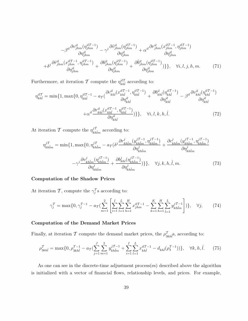
−βil∂vil

jhm(ηilT −1jhm )

∂ηiljhm

− γj∂vil

jhm(ηilT −1jhm )

∂ηiljhm

+ αil∂ril

jhm(xilT −1jhm , ηilT −1

jhm )

∂ηiljhm

+δj ∂riljhm(xilT −1

jhm , ηilT −1jhm )

∂ηiljhm

+∂bil

jhm(ηilT −1jhm )

∂ηiljhm

+∂bil

jhm(ηilT −1jhm )

∂ηiljhm

)}}, ∀i, l, j, h, m. (71)

Furthermore, at iteration T compute the ηilTkhl

according to:

ηilTkhl

= min{1, max{0, ηilT −1

khl− aT (

∂cilkhl

(xilT −1

khl, ηilT −1

khl)

∂ηilkhl

+∂bil

khl(ηilT −1

khl)

∂ηilkhl

− βil∂vil

khl(ηilT −1

khl)

∂ηilkhl

+αil∂ril

khl(xilT −1

khl, ηilT −1

khl)

∂ηilkhl

)}}, ∀i, l, k, h, l. (72)

At iteration T compute the ηjTkhlm

according to:

ηjTkhlm

= min{1, max{0, ηjTkhlm

− aT (δj∂rj

khlm(yjT −1

khlm, ηjT −1

khlm)

∂ηj

khlm

+∂cj

khlm(yjT −1

khlm, ηjT −1

khlm)

∂ηj

khlm

−γj∂vj

khlm(ηjT −1

khlm)

∂ηj

khlm

+∂bj

khl(ηjT −1

khlm)

∂ηj

khlm

)}}, ∀j, k, h, l, m. (73)

Computation of the Shadow Prices

At iteration T , compute the γTj s according to:

γTj = max{0, γT −1

j − aT (2∑

m=1

I∑

i=1

L∑

l=1

H∑

h=1

xilT −1jhm −

K∑

k=1

H∑

h=1

L∑

l=1

yjT −1

khlm

)}, ∀j, (74)

Computation of the Demand Market Prices

Finally, at iteration T compute the demand market prices, the ρT3khl

s, according to:

ρT3khl

= max{0, ρT −1

3khl− aT (

J∑

j=1

2∑

m=1

yjT −1

khlm+

I∑

i=1

L∑

l=1

xilT −1

khl− dkhl(ρ

T −13 ))}, ∀k, h, l. (75)

As one can see in the discrete-time adjustment process(es) described above the algorithm

is initialized with a vector of financial flows, relationship levels, and prices. For example,

39

the relationship levels may be set to zero (and the same holds for the prices, initially). The

financial flows, shadow prices, and the demand market prices are computed in the financial

network of the supernetwork. The financial product transactions between intermediaries

and demand markets are computed according to (70). The relationship levels are computed

in the social network of the supernetwork according to (71), (72), and (73), respectively.

Finally, the shadow prices are computed according to (74) and the demand market prices

are computed according to (75).

The dynamic supernetwork system will then evolve according to the discrete-time ad-

justment process (70) through (75) until a stationary/equilibrium point of the projected dy-

namical system (66) (equivalently, and a solution to variational inequality (54)) is achieved.

Once the convergence tolerance has been reached then the equilibrium conditions according

to Definition 1 are satisfied as one can see from (70) through (75).

In the next Section, we apply the Euler method to solve several international financial

network examples. Convergence results for this algorithm may be found in Dupuis and

Nagurney (1993) and for a variety of applications in Nagurney and Zhang (1996a).

40

5. Numerical Examples

In this section, we applied the Euler method to several supernetwork examples as dis-

cussed in the preceding sections. The Euler method was implemented in FORTRAN and

the computer system used was a Sun system located at the University of Massachusetts

at Amherst. For the solution of the induced network subproblems in the (x1, x2) variables

we utilized the exact equilibration algorithm (see Dafermos and Sparrow (1969), Nagurney

(1999), and the references therein). The other variables were determined explicitly and in

closed form as described in the preceding section.

The convergence criterion used was that the absolute value of the flows, prices, and

relationship levels between two successive iterations differed by no more than 10−4. The

sequence {aT } used for all the examples was: 1, 12, 1

2, 1

3, 1

3, 1

3, . . . in the algorithm.

We assumed in all the examples that the risk was represented through variance-covariance

matrices for both the source agents in the countries and for the financial intermediaries

(see also Nagurney and Cruz (2004)). We initialized the Euler method as follows: We set

xiljh1 = Sil

JHfor each source agent i and country l and for all j and h. All the other variables

were initialized to zero.

Example 1

The first numerical example consisted of one country, two source agents, two currencies,

two intermediaries, and two financial products. Hence, L = 1, I = 2, H = 2, J = 2, and

K = 2. In this example, the electronic transactions were only between the source agents

and the demand markets. In addition, for simplicity, we considerd the possibility of the

existence of relationship levels only between the source agents and the intermediaries, and

the intermediaries and demand markets.

The data for the first example were constructed for easy interpretation purposes. The

financial holdings of the two source agents were: S11 = 20 and S21 = 20. The variance-

covariance matrices were equal to the identity matrices (appropriately dimensioned) for all

source agents and all intermediaries. Note that since only physical transactions are allowed

(except for as stated above), we have that m = 1.

41

The transaction cost functions faced by the source agents associated with transacting

with the intermediaries (cf. (4)) were given by:

ciljhm(xil

jhm, ηiljhm) = .5(xil

jhm)2 + 3.5xiljhm − ηil

jhm; i = 1, 2; l = 1; j = 1, 2; h = 1, 2; m = 1.

The analogous transaction costs but associated with the electronic transactions between

source agents and demand markets (cf. (4)) were given by:

cilkhl

(xilkhl

) = .5(xilkhl

)2 + xkhl; ∀i, l, l, k, h.

Note that here we did not include relationship levels in the functional forms.

The handling costs of the intermediaries, in turn (see (27)), were given by:

cj(x1) = .5(

2∑

i=1

2∑

h=1

xi1jh1)

2; j = 1, 2.

The transaction costs of the intermediaries associated with transacting with the source

agents were (cf. (25)) given by:

ciljhm(xil

jhm, ηiljhm) = 1.5xil

jhm

2+ 3xil

jhm; i = 1, 2; l = 1; j = 1, 2; h = 1, 2; m = 1.

The transaction costs, in turn, associated with the electronic transactions at the demand

markets (from the perspective of the consumers (cf. (48)) were given by:

cilkhl

(x2, y, η2, η3) = .1xilkhl

+ 1, ∀i, l, l, k, h.

The demand functions at the demand markets (refer to (49)) were:

d111(ρ3) = −2ρ3111 − 1.5ρ3121 + 1000, d121(ρ3) = −2ρ3121 − 1.5ρ3111 + 1000,

d211(ρ3) = −2ρ3211 − 1.5ρ3221 + 1000, d221(ρ3) = −2ρ3221 − 1.5ρ3211 + 1000,

and the transaction costs between the intermediaries and the consumers at the demand

markets (see (47)) were given by:

cj

khlm(x2, y, η2, η3) = yj

khlm+ 5 − ηj

khlm; k = 1, 2; h = 1, 2; l = 1; m = 1.

42

The relationship value functions (14) and (38) were given by:

viljhm(ηil

jhm) = ηiljhm, ∀i, l, j, h, m; vj

khlm(ηj

khlm) = ηj

khlm, ∀j, k, h, l, m,

with all other relationship value functions being set equal to zero.

The relationship cost functions (cf. (2) and (24)) were as follows:

biljhm(ηil

jhm) = 2ηiljhm, ∀i, l, j, h, m; bj

khlm(ηj

khlm) = ηj

khlm, ∀j, k, h, l, m.

Since all the weights associated with the criteria were set equal to one this means that the

source agents as well as the intermediaries weight the criterion of risk minimization equally

to that of net revenue maximization and relationship value maximization.

The Euler method converged in 2,998 iterations and yielded the following equilibrium

financial flow pattern:

x1∗ := x11∗111 = x11∗

121 = x11∗211 = x11∗

221 = x21111∗ = x22∗

211 = x21∗211 = x21∗

221 = .0662;

x2∗ := x11∗111 = x11∗

121 = x11∗211 = x11∗

221 = x21∗111 = x21∗

121 = x21∗211 = x21∗

221 = 4.9938;

y∗ := y1∗1111 = y1∗

1211 = y1∗2111 = y1∗

2211 = y2∗1111 = y2∗

1211 = y2∗2111 = y2∗

2211 = .0642.

Both source agents allocated the entirety of their funds to the instrument in the two

currencies; thus, there was no non-investment.

The vector λ∗ had components: λ∗1 = λ∗

2 = 272.7246, and the computed demand prices

at the demand markets were: ρ∗3111 = ρ∗

3121 = ρ∗3211 = ρ∗

3221 = 282.8586.

All the relationship levels were identically equal to zero.

Note that due to the lower transaction costs associated with electronic transactions di-

rectly between the source agents and the demand markets a sizeable portion of the financial

funds were transacted in this manner.

Example 2

Example 2 was constructed from Example 1 as follows. We kept the data the same except

that we increased the weights associated with the relationship levels of the source agents

43

from 1 to 20. Hence, in this example, the source agents weight relationship levels much

higher than in Example 1. The Euler method again converged requiring the same number of

iterations as in Example 1, but now the relationship levels of all the source agents increased

to the maximum possible value of 1. All other computed equilibrium values remained as in

Example 1.

Example 3

The third example consisted of two countries with two source agents in each country; two

currencies, two intermediaries, and two financial products. Hence, L = 2, I = 2, H = 2,

J = 2, and K = 2.

The data for Example 3 was constructed for easy interpretation purposes and to create

a baseline from which additional simulations could be conducted. In fact, we essentially

“replicated” the data for the first country as it appeared in Example 1 in order to construct

the data for the second country.

Specifically, the financial holdings of the source agents were: S11 = 20, S21 = 20, S12 =

20, and S22 = 20. The variance-covariance matrices were equal to the identity matrices

(appropriately dimensioned) for all source agents in each country and for all intermediaries,

respectively.

The transaction cost functions faced by the source agents associated with transacting

with the intermediaries were given by:

ciljhm(xil

jhm, ηiljhm) = .5(xil

jhm)2 + 3.5xiljhm − ηil

jhm; i = 1, 2; l = 1, 2; j = 1, 2; h = 1, 2; m = 1.

The handling costs of the intermediaries (since the number of intermediaries is still equal

to two) remained as in Example 1, that is, they were given by:

cj(x1) = .5(

2∑

i=1

2∑

h=1

xi1jh1)

2; j = 1, 2.

The transaction costs of the intermediaries associated with transacting with the source

agents in the two countries were given by:

ciljhm(xil

jhm) = 1.5(xiljhm)2 + 3xil

jhm; i = 1, 2; l = 1, 2; j = 1, 2; h = 1, 2; m = 1.

44

The demand functions at the demand markets were:

d111(ρ3) = −2ρ3111 − 1.5ρ3121 + 1000, d121(ρ3) = −2ρ3121 − 1.5ρ3111 + 1000,

d211(ρ3) = −2ρ3211 − 1.5ρ3221 + 1000, d221(ρ3) = −2ρ3221 − 1.5ρ3211 + 1000,

d112(ρ3) = −2ρ3112 − 1.5ρ3122 + 1000, d122(ρ3) = −2ρ3122 − 1.5ρ3112 + 1000,

d212(ρ3) = −2ρ3212 − 1.5ρ3222 + 1000, d222(ρ3) = −2ρ3222 − 1.5ρ3212 + 1000,

and the transaction costs between the intermediaries and the consumers at the demand

markets were given by:

cj

khl(yj

khlm, ηj

khlm) = yj

khl− ηj

khl+ 5; j = 1, 2; k = 1, 2; h = 1, 2; l = 1, 2; m = 1.

The data for the electronic links were as in Example 1 and were replicated for the other

source agents.

The variance-covariance matrices were redimensioned and were equal to the identity ma-

trices. The weights associated with the risk functions were set equal to 1 for all the source

agents and intermediaries.

The Euler method converged in 1,826 iterations and yielded the following equilibrium

international financial flow pattern: only the electronic links had positive flows with all

other flows being identically equal to 0.000. In particular, the financial holdings of the

source agents in the different countries were equally allocated via electronic transactions

directly to the demand markets with xil∗khl

= 2.5000 for all i, l, k, h, l.

The vector λ∗ had components: λ∗1 = λ∗

2 = 279.6194, and the computed demand prices

at the demand markets were: ρ∗3khl

= 282.8578, ∀k, h, l. In this example, all the financial

transactions were conducted electronically.

Example 4

Example 4 was constructed from Example 3 in a similar manner to that in which Example

2 was constructed from Example 1. In other words, we now increased the weight associated

with all the source agents in boths countries from 1 to 20 regarding the criterion of rela-

tionship value maximization. The equilibrium pattern computed by the Euler method was

45

identical to that obtained for Example 3 but now the relationship values associated with the

source agents were all equal to their upper bound with a value of 1.

These examples, although stylized, have been presented to show both the model and the

computational procedure. Obviously, different input data and dimensions of the problems

solved will affect the equilibrium financial flow, price, and relationship level patterns. One

now has a powerful tool with which to explore the effects of perturbations to the data as

well as the effects of changes in the number of source agents, countries, currencies, and/or

products, as well as the effects of the introduction of electronic transactions. Morever,

this supernetwork framework allows for the tracking of the co-evolution of the international

financial flows, the product prices, as well as the relationship levels over space and time.

46

6. Summary and Conclusions

In this paper, we developed a supernetwork model that integrated international financial

networks with intermediation with social networks in which relationship levels were made

explicit. Both networks had three tiers of decision-makers, consisting of: the sources of

financial funds in the countries, the financial intermediaries, and the consumers associated

with the demand markets for the financial products. We allowed for physical as well as

electronic transactions between the decision-makers in the supernetwork. The relationship

levels were allowed to affect not only the risk but also the transaction costs (by reducing

them, in general) but did have associated costs. Moreover, we allowed for multicriteria

decision-making behavior in which the source agents as well as the financial intermediaries

were permitted to weight, in an individual fashion, their objective functions of net revenue

maximization, total risk minimization, and total relationship value maximization.

We modeled the supernetwork in equilibrium, in which the international financial flows

between the tiers as well as the relationship levels coincide and established the variational

inequality formulation of the governing equilibrium conditions. We then proposed the un-

derlying dynamics and the continuous-time adjusrtment process(es) and constructed its pro-

jected dynamical system representation. We established that the set of stationary points

of the projected dynamical system coincides with the set of solutions of the variational in-

equality problem. We also provided conditions under which the dynamic trajectories of the

financial flows, relationship levels, and prices are well-defined.

We proposed a discrete-time algorithm to approximate the continuous-time adjustment

process and applied it to several simple numerical examples for completeness and illustrative

purposes. The framework developed here further advances the work in financial equilibrium

modeling and analysis, especially within a network context by explicitly considering the

effect of relationship levels in financial networks and by establishing the optimal relationship

levels as well as financial transaction quantities and prices. Finally, it also gives us insight

into the optimal designs of the supernetworks.

This framework generalizes the recent work of Nagurney, Wakolbinger, and Zhao (2004)

in the evolution and emergence of integrated social and financial networks with electronic

transactions to the international dimension. In addition, it incorporates social networks into

47

the international financial network framework of Nagurney and Cruz (2003).

Acknowledgments

This research was supported, in part, by NSF Grant No.: IIS-0002647 and, in part, by an

AT&T Industrial Ecology Fellowship. This support is gratefully acknowledged.

References

Anthony, D. L. (1997), “Micro-Lending Institutions: Using Social Networks to Create Pro-

ductive Capabilities,” International Journal of Sociology and Social Policy 17, 156-178.

Arrow, K. J. (1998), “What has Economics to Say about Racial Discrimination?” Journal

of Economic Perspectives 12, 91-100.

Bazaraa, M. S., Sherali, H. D. and Shetty, C. M. (1993), Nonlinear Programming: Theory

and Algorithms, John Wiley & Sons, New York.

Claessens, S. (2003), “Benefits and Costs of Integrated Financial Services Provision,” Forth-

coming in R. E. Litan and R. Herring, Editors, Brookings-Wharton Papers on Financial

Services 2002, The Brookings Institution, Washington, DC.

Claessens, S., Glaessner, T. and Klingebiel, D. (2000), “Electronic Finance: Reshaping the

Financial Landscape Around the World,” Financial Sector Discussion Paper No. 4, The

World Bank, Washington, DC.

Claessens, S., Glaessner, T. and Klingebiel, D. (2001), “E-Finance in Emerging Markets:

Is Leapfrogging Possible?” Financial Sector Discussion Paper No. 7, The World Bank,

Washington, DC.

Claessens, S., Dobos, G., Klingebiel, D. and Laeven, L. (2003), “The Growing Importance

of Networks in Finance and Their Effects on Competition,” in Innovations in Financial and

Economic Networks, A. Nagurney, Editor, Edward Elgar Publishers, Cheltenham, England,

pp. 110-135.

Dafermos, S. and Sparrow, F. T. (1969), “The Traffic Assignment Problem for a General

48

Network,” Journal of Research of the National Bureau of Standards 73B, 91-118.

DiMaggio, P. and Louch, H. (1998), “Socially Embedded Consumer Transactions: For What

Kinds of Purchases Do People Most Often Use Networks,” American Sociological Review 69,

619-637.

Dong, J., Zhang, D. and Nagurney, A. (2002), “Supply Chain Networks with Multicriteria

Decision-Makers,” in Transportation and Traffic Theory in the 21st Century , M. A. P. Taylor,

Editor, Pergamon, The Netherlands.

Dupuis, P. and Nagurney, A. (1993), “Dynamical Systmes and Variational Inequalities,”

Annals of Operations Research 44, 9-42.

G-10 (2001), “Report on Consolidation in Financial Sector,” Bank for International Settle-

ments, Switzerland.

Gabay, D. and Moulin, H. (1980), “On the Uniqueness and Stability of Nash Equilibria in

Noncooperative Games,” in Applied Stochastic Control of Econometrics and Management

Science, A. Bensoussan, P. Kleindorfer, and C. S. Tapiero, Editors, North-Holland, Amster-

dam, The Netherlands, pp. 271-294.

Ghatak, M. (2002), “Exploiting Social Networks to Alleviate Credit Market Failures: On

the Engogenous Selection of Peer Groups in Microfinance Programs,” Prepared for the Con-

ference on Credit, Trust and Calculation at the University of California.

Keeney, R. L. and Raiffa, H. (1993), Decisions with Multiple Objectives: Preferences and

Value Tradeoffs, Cambridge University Press, Cambridge, England.

Kim, H. M. (1999), Globalization of International Financial Markets, Ashgate, Hants, Eng-

land.

Markowitz, H. M. (1952), “Portfolio Selection,” The Jounral of Finance 7, 77-91.

Markowitz, H. M. (1959), Portfolio Selection: Efficient Diversification of Investments, John

Wiley & Sons, Inc., New York.

49

Nagurney, A. (1999), Network Economics: A Variational Inequality Approach, Second and

Revised Edition, Kluwer Academic Publishers, Dordrecht, The Netherlands.

Nagurney, A., Editor (2003), Innovations in Financial and Economic Networks, Edward

Elgar Publishing, Cheltenham, England.

Nagurney, A. and Cruz, J. (2003), “International Financial Networks with Electronic Trans-

actions,” in Innovations in Financial and Economic Networks, A. Nagurney, Editor, Edward

Elgar Publishers, Cheltenham, England, pp. 136-168.

Nagurney, A. and Cruz, J. (2004), “Dynamics of International Financial Networks with Risk

Management,” Quantitative Finance 4, 276-291.

Nagurney, A., Cruz, J. and Matsypura, D. (2003), “Dynamics of Global Supply Chain Su-

pernetworks,” Mathematical and Computer Modelling 37, 963-983.

Nagurney, A. and Dong, J. (2002), Supernetworks: Decision-Making for the Information

Age, Edward Elgar Publishers, Cheltenham, England.

Nagurney, A. and Ke, K. (2001), “Financial Networks with Intermediation,” Quantitative

Finance 1, 441-451.

Nagurney, A. and Ke, K. (2003), “Financial Networks with Electronic Transactions: Mod-

eling, Analysis, and Computations,” Quantitative Finance 3, 71-87.

Nagurney, A. and Siokos, S. (1997), Financial Networks: Statics and Dynamics, Springer-

Verlag, Heidelberg, Germany.

Nagurney, A., Wakolbinger, T. and Zhao, L. (2004), “The Evolution and Emergence of

Integrated Social and Financial Networks with Electronic Transactions: A Dynamic Super-

network Theory for the Modeling, Analysis, and Computation of Financial Flows and Re-

lationship Levels,” Isenberg School of Management, University of Massachusetts, Amherst;

http://supernet.som.umass.edu

Nagurney, A. and Zhang, D. (1996a) Projected Dynamical Systems and Variational Inequal-

50

ities with Applications, Kluwer Academic Publishers, Dordrecht, The Netherlands.

Nagurney, A. and Zhang, D. (1996b), “Stability of Spatial Price Equilibrium Modeled as a

Projected Dynamical System,” Journal of Economic Dynamica and Control 20, 43-63.

Nagurney, A. and Zhang, D. (1997), “Formulation, Stability, and Computation of Traffic

Network Equilibria as Projected Dynamical Systems,” Journal of Optimization Theory and

its Applications 93, 417-444.

Nash, J. F. (1950), “Equilibrium Points in N-Person Games,” in Proceedings of the National

Academy of Sciences, USA 36, 48-49.

Nash, J. F. (1951), “Noncooperative Games,” Annals of Mathematics 54, 286-298.

Sharpe, S. A. (1990), “Asymmatric Information, Bank Lending, and Implicit Contracts: A

Stylized Model of Customer Relationships,” The Journal of Finance 45, 1069-1085.

Uzzi, B. (1997), “Social Structure and Competition in Interfirm Networks: The paradox of

Embeddedness,” Administrative Science Quarterly 42, 35-67.

Uzzi, B. (1999), “Embeddedness in the Making of Financial Capital: How Social Relations

and Networks Benefit Firms Seeking Financing,” American Sociological Review 64, 481-505.

Wakolbinger, T. and Nagurney, A.(2004), “Dynamic Supernetworks for the Integration of

Social Networks and Supply Chains with Electronic Commerce: Modeling and Analysis of

Buyer-Seller Relationships with Computations,” Isenberg School of Management, University

of Massachusetts, Amherst; http://supernet.som.umass.edu

Zhang, D. and Nagurney, A. (1995), “On the Stability of Projected Dynamical Systems,”

Journal of Optimization Theory and its Applications 85, 97-124.

51