the choice between real and accounting earnings …the choice between real and accounting earnings...

The Choice between Real and Accounting Earnings Management

Jeff Z. Chen

Department of Accountancy and Taxation

C.T. Bauer College of Business

University of Houston

Houston, TX 77004

Tel: 713-743-4887

[email protected]

Job market paper

February 2009

This paper is based on my dissertation at the University of Houston. I am indebted to my commit members,

Tong Lu, Lynn Rees, Ron Singer, Scott Whisenant, K. Sivaramakrishnan (co-chair) and Gerald Lobo (co-

chair) for their guidance and encouragement. I also thank seminar participants at the University of Houston

for helpful comments. All errors are my own.


ABSTRACT

This study develops a theoretical model and presents empirical evidence on cross-

sectional variation in managers’ choice of AEM and REM. In particular, it studies how

AEM and REM are jointly affected by firms’ growth prospects, managers’ market-based

compensation incentives, and the cost of real earnings management. The model yields

several testable hypotheses. First, when the firm’s growth prospects are good, the firm

will boost current period earnings through AEM, but not REM. Second, when the

sensitivity of the manager’s compensation to stock price and/or value-relevance of

earnings go up, the firm will use AEM, but not REM, to inflate current period earnings.

Third, when the cost of REM increases, the manager will reduce opportunistic excess

investment. Meanwhile, AEM decreases in the cost of REM. Firms that barely meet or

beat analysts’ forecasts are used to test the model’s predictions. The results are in general

consistent with the hypotheses.

1


1. Introduction

There is substantial evidence that managers engage in accounting earnings

management (hereafter, AEM) and/or real earnings management (hereafter, REM) to

achieve certain earnings targets (Burgstahler and Dichev 1997; Burgstahler and Eames

2006; Roychowdhury 2006; Chen et al. 2008). AEM refers to managers’ opportunistic

use of the flexibility allowed under General Accepted Accounting Principles (GAAP) to

change reported earnings without changing the underlying cash flows. REM refers to

managers’ opportunistic timing and structuring of operating, investment and financing

transactions to affect reported earnings in a particular direction; it results in sub-optimal

business consequences and imposes a real cost on the firm. This study develops a

theoretical model and presents empirical evidence on cross-sectional variation in

managers’ choice of AEM and REM. In particular, it studies how AEM and REM are

jointly affected by firms’ growth prospects, managers’ market-based compensation

incentives, and the cost of real earnings management.

There is relatively little analytical investigation and some mixed empirical

evidence on how managers choose between AEM and REM. On the one hand, evidence

from earnings distributions suggests that managers use both AEM and REM to meet

earnings targets. For example, Burgstahler and Dichev (1997) find that both cash flow

from operations and changes in current accruals are managed to increase earnings, and

Burgstahler and Eames (2006) document that both cash flow from operations and

discretionary accruals are managed upwards to avoid reporting earnings lower than

analyst forecasts. On the other hand, Zang (2007) provides large sample evidence that

managers trade off using AEM and REM to achieve their objectives. Relatedly, Barton

(2001) and Pincus and Rajgopal (2002) present evidence that managers use derivatives

and discretionary accruals as partial substitutes for smoothing earnings. While these

studies attempt to examine the link between AEM and REM by correlating these two

decision variables, a more thorough and comprehensive approach to investigate managers’

choice of REM and AEM is to examine their relation to exogenous firm or manager

2

characteristics. This study attempts to fill that void in the earnings management literature

in an effort to advance our understanding of managers’ financial reporting behavior.

Earnings management decisions critically hinge on a firm’s growth prospects,

management compensation incentives, and cost of real activities manipulation. Firms in

different life cycle stages have different prospects for economic growth. Graham et al.

(2005) report survey evidence that managers of growing firms engage in earnings

management because they expect future earnings growth to offset reversals from past

earnings management decisions. They also believe that if the firm’s financial condition

continues to deteriorate, even small earnings management decisions can cascade and lead

to negative consequences in later periods. Starting with Healy (1985), many studies argue

that managers exercise their accounting discretion to maximize their compensation (e.g.,

Cheng and Warfield 2005; Bergstresser and Philippon 2006). However, there is little

evidence on the relation between management compensation incentives and REM, and its

trade-off against AEM. Zang (2007) and Ewert and Wagenhofer (2005) argue that real

and accounting manipulation are substitutes in the cost of accounting manipulation.

However, compared to real activities manipulation, within-GAAP discretionary

accounting choices are less costly and less resource-consuming, suggesting that the cost

of real manipulation is a critical element of a manager’s decision making process.

This study first develops a parsimonious model for analyzing a manager’s

earnings management decisions in a capital market setting, assuming the manager is

interested in both current stock price and long-term earnings growth. The model yields

several testable hypotheses. First, when the firm’s growth prospects are good, the firm

will boost current period earnings through AEM, but not REM. Meanwhile, it will

opportunistically increase the level of investment in order to report higher future earnings.

Second, when the sensitivity of the manager’s compensation to stock price and/or market

pricing of earnings goes up, the firm will use AEM, but not REM, to inflate current

period earnings. The manager will opportunistically increase investment in the first

period to boost future earnings and dampen the adverse effect of AEM unwinding in the

second period. Third, when the cost of REM is high, the manager will reduce

opportunistic excess investment. Current earnings will increase as a result of the decrease

in overinvestment. While it appears that the manager is cutting investment expenditure

3

and inflating current period earnings to boost earnings, a phenomenon consistent with

using REM, AEM decreases in the cost of REM. As the manager reduces opportunistic

investment in the first period, his long-term incentive to report growing earnings may

result in the use of AEM to save earnings for the future.

Testing the model’s predictions requires a setting in which the incentives to

deliver short-term earnings and maximize long-term firm value dominate other

confounding factors that could also impact the manager’s AEM and REM choices. I use a

sample of firms that barely meet or beat annual analysts’ earnings forecasts (hereafter

MBE) to test the model’s predictions. The potential to garner market rewards to MBE

induces managers who are concerned about short-term stock price performance to report

earnings that MBE (Lopez and Rees 2002; Bartov et al. 2002; Lin et al. 2006; Chen et al.

2008). Meanwhile, managers are also interested in the firm’s long-term financial

performance. If they exhaust their ability to optimistically bias earnings to achieve short-

term earnings targets, the likelihood of reporting earnings that MBE in the future will

decrease (Barton and Simko 2002). Concern about future performance (or MBE in the

future) may partially explain why a disproportionate number of firms report only one or

two cents of earnings surprise.1 Although my model does not directly examine MBE

behavior per se, it has strong empirical implications in this setting.

I identify firms that meet or just beat consensus analyst forecasts, i.e., earnings

surprise greater than or equal to zero, but less than 2 cents, as suspect firms because it is

more likely that these firms engage in REM and AEM to achieve their earnings targets

(Roychowdhury 2006). I then perform univariate portfolio analyses and multivariate

regression analyses to test the model’s predictions. In general, I find empirical evidence

consistent with the hypotheses. AEM increases with a firm’s growth prospects, indicating

that growth firms are more likely to use AEM to boost earnings and MBE. REM

decreases with a firm’s growth prospects, suggesting that firms are less likely to use

REM to MBE and more interested in the long-term effect of investment. I also find strong

1 Earnings management induced by managers’ incentive to garner short-term stock market rewards to MBE

and their interest in smoothing earnings inter-temporally also catches regulators’ attention. For example,

Arthur Levitt, then SEC chief commissioner, in his 1998 “The Numbers Game” speech, stated

“Increasingly, I have become concerned that the motivation to meet Wall Street earnings expectations may

be overriding common sense business practices… In the zeal to satisfy consensus earnings estimates and

project a smooth earnings path, wishful thinking may be winning the day over faithful representation.”

(emphasis added)

4

evidence that AEM increases with the sensitivity of a manager’s stock-based

compensation to stock price and market pricing of earnings. Matsumoto (2002) reports

similar findings, except that she only focuses on AEM behavior in the MBE setting.

Consistent with the prediction that firms will “save” for future earnings by investing

more today, I find that REM is less likely to be used to MBE (or equivalently,

opportunistic investment is more likely to increase) as the sensitivity of manager’s stock-

based compensation to stock price and market pricing of earnings increase. I find support

for the prediction that AEM decreases with the cost of REM. However, I do not detect a

significant relation between REM and its own cost. One explanation for this weak

evidence is that my proxy for REM cost is too noisy.

My study contributes to the literature in the following ways. First, Graham et al.

(2005) document surprising and disturbing results that the majority of managers admit to

sacrificing long-term economic value, such as cutting R&D, delaying maintenance or

advertising expenditure, even giving up positive NPV projects, to hit a target or to

smooth short-term earnings. Why managers seem to be more reluctant to employ within-

GAAP accounting discretion to meet earnings targets when it likely is less costly than the

loss in economic value resulting from real earnings management remains a puzzling

question. Graham et al. conjecture that the tendency to substitute real economic actions

for accounting discretion might be a consequence of higher cost of accounting fraud in

the post-Enron era. My model shows that other determinants such as a firm’s growth

prospects and compensation sensitivity to stock price may also affect the choice of AEM

and REM. In this regard, I provide some potential explanations for the puzzle

documented in Graham et al. (2005).

Next, as suggested by Fields et al. (2001), examining only one earnings

management technique at a time for one purpose may not explain the overall effect of

earnings management activities. In particular, if managers use AEM and REM to

accomplish the same objective, examining one type of manipulation in isolation may lead

to an understatement of the overall level of earnings management. If managers’ use of

AEM and REM is offsetting, focusing on either type of manipulation at a time for one

purpose will only provide partial evidence and perhaps result in incorrect conclusions.

For example, prior studies find that managers boost earnings through discretionary

5

accruals when their compensation is more closely tied to stock prices. However, total

earnings management may not be as prominent as researchers would expect, because

managers may use real activities manipulation in the opposite direction to accomplish a

conflicting earnings management goal.

Third, Matsumoto (2002) examines the effect of certain firm characteristics on the

likelihood of firms to MBE. Her study focuses on cross-sectional differences in the

incentives to MBE, whereas my study addresses cross-sectional variation in the means of

MBE. In that regard, my study can be viewed as an extension of or a complement to

Matsumoto (2002).

Fourth, by studying how managers use both real and accounting manipulations to

manage earnings, my paper sheds light on the implications of whether improving

corporate governance or reducing accounting flexibility in GAAP might improve overall

resource allocation in the capital market. As suggested by Graham et al. (2005), managers’

preference for using real activities manipulation over less costly accrual manipulation

suggests a flaw in corporate governance practices. Since most recent attention on

improving corporate governance only focuses on reducing accounting manipulation, my

paper suggests that it is also important to improve the effectiveness of managers’ real

decisions. Relying on the corporate governance mechanism alone to restrict accounting

earnings management may not necessarily lead to an improvement in resource allocation

in the capital market.

The paper proceeds as follows: Section 2 presents the theoretical model and its

predictions. Section 3 discusses the empirical implications of the model and selection of

empirical setting. Section 4 constructs the proxies for REM and AEM. Section 5 contains

main empirical results. Section 6 concludes this study.

2. Model and Research Hypotheses

As discussed earlier, recent survey evidence reported in Graham et al. (2005)

indicates that managers would rather take economic actions that could have negative

long-term consequences than risk attracting regulatory scrutiny by making within-GAAP

6

accounting choices to manage earnings.2 Eighty percent of survey participants admit that

they would decrease discretionary spending on R&D, advertising and maintenance to

achieve desired earnings levels; fifty-five percent indicate that they would delay starting a

new project to meet an earnings target, even if such a decision sacrificed firm value. Most

surveyed managers acknowledge that they face a trade-off between delivering short-run

earnings and making long-run optimal decisions.

In this section, I develop a model that describes how managers choose between

real and accounting earnings management in a capital market setting when they face both

short-run and long-run incentives. The purpose of the model is to provide a theoretical

framework for analyzing the interactions between the manager’s AEM and REM

decisions and the capital market’s pricing of the firm, and to generate testable

implications.

The model spans two periods and includes a risk-neutral manager of a firm that

operates in a competitive risk-neutral capital market. In the first period, the manager

decides how much to spend on discretionary expenditures. Then, based on realized and

privately observed outcomes of his real decisions, the manager makes an AEM decision

and reports potentially biased earnings. The capital market prices the firm based on the

reported earnings. In the second period, the earnings management effect unwinds and the

firm is liquidated. In the spirit of Ewert and Wagenhofer (2005), I assume the manager is

concerned about both stock price and reported earnings growth, i.e., the manager has

some interest in both the short-term and the long-term effects of earnings management.

The model has several salient features. First, it focuses on the manager’s trade-off

between the short-term interest in stock price and the long-term objective of earnings

growth. Second, it captures the sequentiality of REM and AEM decisions (Zang 2007;

Chen et al. 2008). Third, it examines the impact of key firm characteristics on earnings

management decisions. Finally, the model allows the marginal benefits of REM and

AEM to differ (both in the short-run and in the long-run). This differs from prior studies

which assume that the marginal benefits of REM and AEM are the same (Zang 2007), a

2 Graham et al. suggest that the accounting scandals at Enron and WorldCom’s and the subsequent

certification requirements imposed by the Sarbanes-Oxley Act may have changed managers’ preferences

for the mix between taking accounting versus real actions to manage earnings. Another possible

explanation is that managers are simply more willing to manage earnings through real decisions than

through accounting decisions (Cohen et al. 2008).

7

limiting assumption that suppresses the key difference between real decisions and

accounting decisions.3

Manager’s real decisions

I begin with the manager first deciding how much to spend on a real decision that

yields a return K in the first period, and γK in the second period (γ > 0). The parameter γ

captures the growth prospects of the firm. A larger γ indicates stronger growth prospects

and higher return in the second period. Let cK2/2 denote the firm’s expenditure on K,

where K is the manager’s private information and c is an exogenous and positive constant.

REM implies that the manager departs from the first best decision only to alter

earnings (Ewert and Wagenhofer, 2005). REM is inefficient and imposes real costs on the

firm. If KFB

is the first best level of discretionary expenditure and K* the manager’s actual

choice, then the level of REM may be expressed as bR = KFB

– K*. I assume that the cost

of REM is εbR2/2, where ε (ε ≥ 0) is an exogenous cost parameter.

4 Strictly speaking,

however, the cost of REM should be endogenous rather than imposed exogenously in the

model. Nevertheless, following Ewert and Wagenhofer (2005), I explicitly model the cost

of REM and assume it is incurred in the second period. One way of rationalizing this

structure is to recognize that, in practice, the contracting process is not always complete

and does not efficiently incorporate all relevant information (i.e., with respect to the costs

of REM).5

The accounting system

The firm implements an accounting system that records transactions and events as

a result of the manager’s real decisions. The unmanaged earnings in period 1, x1 is

assumed to be distributed uniformly within [K - cK2/2 - ε, K - cK

2/2 +ε], where ε > 0. In

3 The following example highlights this difference. Assuming the marginal rate of return on an investment

project is 10% and the manager makes a real decision to reduce this investment by $1, he saves $1 on

expenditures but also suffers a loss in revenue of $0.10. The net impact is a $0.90 increase in earnings. On

the other hand, a $1 increase in AEM results in a $1 increase in earnings. 4 Note that Ewert and Wagenhofer (2005) model these costs as a linear function of bR. Since ex ante, I

allow bR to be either positive or negative (i.e., over- or under- spending on discretionary expenditures), I

model these costs as a quadratic function of bR. 5 This incompleteness assumption is similar in spirit to the non-incorporation of off-balance sheet debt in

debt contracting. As we know, off-balance sheet financing has mushroomed over the last two decades.

8

the second period, the manager does not make any real or accounting earnings

management decisions. He privately observes x2, which is uniformly distributed within

[γK - εbR2/2 - ε, γK - εbR

2/2 + ε], conditional on the level of REM, i.e., bR.

After the manager privately observes the realized earnings signal x1 in period 1, he

issues a public accounting report, m1, about earnings. The report may deviate from the

underlying x1 because the manager can engage in AEM. Let bA denote the level of AEM.

The manager reports m1 in the following way: m1 = x1 + bA. I do not include out-of-pocket

costs of AEM in the model.6 However, accrual reversal against future earnings imposes

nontrivial implicit costs to AEM. AEM unwinds in period 2 and the manager reports m2

as: m2 = x2 - bA. Ex ante, it is not clear whether the cost of REM is greater than the cost of

AEM.

Market price

Let P be the stock price of the firm at the end of the first period.7 Because I

assume a competitive capital market, the stock price equals the market’s expected total

cash flows generated by the firm, i.e. P = 121

mxxE .

The manager’s utility

The manager’s compensation typically includes both an annual bonus plan and a

long-term incentive plan. Much of the analytical and empirical research focuses on

accounting earnings and stock prices as key performance measures (Bushman and Smith

2001; Bushman et al. 1998, 2001; Core et al. 2003; Jensen and Murphy 1990; Kaplan

6 According to Marquardt and Wiedman (2004), the costs of accounting earnings management can be

classified into two groups: the costs of detected earnings management and the costs of undetected earnings

management. Detected earnings management refers to instances where a firm’s use of earnings

management becomes publicly known, which usually results in one or more of the following consequences:

the release of SEC enforcement actions, earnings restatements, shareholder litigation, qualified audit

opinion, or managers’ reputation loss. I do not include these costs in the model because I am mainly

interested in earnings management within GAAP. Modeling violations of GAAP is beyond the scope of

this study. The most obvious cost of undetected earnings management is its eventual reversal and its impact

on future reported earnings, which I incorporate into the model. Other costs of undetected earnings

management include constraints on future reporting flexibility, audit costs, perceived reduction in earnings

quality, and increased probability of detection. 7 For simplicity, I do not include P2 in the manager’s utility function. The key to the model is that, in t =1,

the manager has some interest in the long-term effects of earnings management, which I capture through

the accounting report m2 in his two-period utility. If the manager’s utility depends on P2 but not on m2, the

results should be qualitatively unchanged as m2 and P2 are linearly dependent in equilibrium.

9

1994; Lambert and Larcker 1987; Sloan 1993; Davila and Penalva 2006). In this model, I

assume the manager’s utility function depends on the firm’s market price (i.e., short-term

incentive) and future earnings growth (i.e., long-term incentive). The manager’s interest

in earnings growth is well documented in the literature (e.g. Myers et al. 2007; Barth et al.

1999; Beatty et al. 2002; Skinner and Sloan 2002; Burgstahler and Dichev 1997; Graham

et al. 2005). The manager’s interest in the firm’s market price may stem from his

intention to sell shares he owns or from an explicit stock-based incentive contract (e.g.

Cheng and Warfield 2005; Bergstresser and Philippon 2006; Bartov and Mohanram

2004). The manager’s two-period utility function is specified as:

2 )(

0 2

2121

21 K

mmifmm

mmifpPU

where p (p >0) denotes the sensitivity of the manager’s compensation to the market price

P. I normalize the sensitivity of his compensation to earnings growth to be one. 8 Thus, p

can be interpreted as the weight the manager places on current market price relative to the

weight on future earnings growth. The key to this utility function is that the manager has

to trade off his interests in the short-term with the long-term effects of earnings

management. On one hand, he has an incentive to manage m1 upward in order to get a

higher P1; on the other hand, because of the reversal of AEM and the cost of REM in t =

2, he is also concerned about the penalty of earnings decrease. Or equivalently, he has

some interest in saving m1 in order to be able to report a higher m2. I include K2/2 to

capture the manager’s disutility of making a real decision.9

8 I assume p to be common knowledge, because information about the management compensation package

is publicly available. In principle, there can be uncertainty with respect to p. However, including

uncertainty would only increase the complexity of the analysis without yielding additional insights. Also,

see Davila and Penalva (2006) for a detailed discussion on the weights of firm performance measures in

CEO compensation. 9 I do not include disutility of the manager’s accounting choice in his utility function. As indicated in

footnote 19 in Graham et al. (2005), managers believe while it is preferable to manage earnings via real

actions rather than accounting choices, it is also more difficult. They must understand the operations up and

down the organization to effectively manage earnings via real actions. One CFO refers to earnings

management via accounting actions as “laziness on the part of the CFO” because much more effort is

necessary to understand all aspects of the business in order to manage earnings via real actions.

10

Figure 1 summarizes the sequence of events

Figure 1

Sequence of Events

Period 1 Period 2

The manager He privately The manager Market price He privately He reports m2 The firm

makes a real observes x1 chooses bA and P observes x2 liquidates

decision reports m1

about K

The first best accounting and real decisions

It is useful to begin with the solution under the first best setting in which the

capital market observes xt and there is no interest misalignment. In this setting, there is no

incentive for the manager to engage in any form of earnings management. The manager

will truthfully report earnings (i.e., x1 = m1) and make real decisions such that firm value

is maximized.

The first best accounting decision is used as the benchmark for comparison with

the level of AEM. In the model, AEM is purely opportunistic and only adds noise to m1.

Therefore, the first best accounting choice, bAFB

, should be 0. Similarly, the first best real

decision, KFB

, is the base for comparison with the level of REM. It is straightforward to

show that KFB

is given by (1+γ)/(1+c).

Equilibrium

I now turn to the setting in which there is both information asymmetry and

incentive misalignment. The manager selects AEM that maximizes his expected utility.

Lemma 1: Given the realized x1, common knowledge c, p, ε, γ, ε, and the conjecture of

the market price reaction to the reported earnings, )(ˆ1

mP , the manager will choose the

level of AEM, bA, as:10

10

All proofs are shown in the Appendix.

11

)2

(2

1)( 2

1

RA bKxpKb

where β is 11

/)(ˆ dmmPd (i.e., the market pricing of earnings) and bA* denotes the optimal

level of AEM.

Lemma 2: Given bA*(K), the manager’s real decision K and REM are based on common

knowledge c, p, ε, γ, ε, and the conjecture of the market price reaction to the reported

earnings, )(ˆ1

mP . He will choose the real decision K*

and the REM level bR* as:

)(2

2

1

1 and

)(2

1

)1(1

*

cp

p

cKKb

cp

cp

K FBR

REM is the deviation of the manager’s choice K* from the first best decision K

FB.

The capital market rationally conjectures the manager’s decisions and prices the

firm accordingly. The price P equals the expected terminal value of the firm given the

manager’s report and the conjectured managerial decisions. In equilibrium, the

conjectured managerial decisions must equal the actual decisions; therefore, the market

price can be derived as:

2 )21(

1

andp where α

mP

β is positive, indicating that the report m1 is relevant for pricing. More importantly,

β is greater than 1. Notice that through the choice of m1 the manager is in essence shifting

income from period 1 to period 2. In a rational equilibrium, the capital market will place

a greater-than-one weight, β, on the reported m1 to figure out x1.

Comparative statics and research hypotheses

From Lemma 2, it is easy to show that, in equilibrium, the manager will over-

(under-) invest on K, relative to KFB

, if p is greater (less) than one. Since b

R is defined as

the difference between the manager’s choice of K and KFB

, its sign depends on the level

of p. More critically, the effects of exogenous firm characteristics, such as γ, p and ε, on

bR will be conditional upon the level of p as well.

For the purpose of this study, I focus on the range of 1< p < ))(1()1(

)1()1(

cc

c in

the following comparative statics analyses. The lower limit of p is one, indicating that the

12

manager’s stock-based incentives outweigh his earnings-based incentives (or equivalently,

short-term incentives outweigh long-term incentives). Recall that under this condition,

the equilibrium bR is negative (i.e., the manager over-invests on K). I set an upper limit

for p, indicating that the manager’s stock-based incentives must be bounded; otherwise

long-term incentives might become trivial. I focus my discussion of the comparative

statics results over this range of p. It has important implications for the MBE

phenomenon that I investigate in the next section. I apply the model’s predictions in a

setting in which firms meet or just beat annual analyst earnings forecasts. The incentive

to MBE arises from managers’ short-term equity market considerations (Abarbanell and

Lehavy 2003). Meanwhile, managers are also concerned about firms’ long-term financial

performance. If they exhausted their ability to optimistically bias earnings to achieve

short-run earnings targets, the likelihood of reporting earnings that MBE in the future

would decrease (Barton and Simko 2002). The concern about future performance may

partially explain why a disproportionate number of firms report only one or two cents of

earnings surprise. Although my model does not directly examine the MBE behavior per

se, it is applicable to this setting.11

If 1< p <))(1()1(

)1()1(

cc

c , the following comparative statics can be derived.

Result 1:

0

0

d

db

d

db

A

R

(1)

When the firm’s growth prospects are stronger, it is natural to expect an increase

in the first-best choice of investment level (KFB

). However, it is not clear how the

manager’s (optimal) choice of investment level (K*) will change in the presence of

information asymmetry and interest misalignment. My model predicts that both the first-

best and the manager’s (optimal) choice of investment level will increase in the firm’s

growth prospects. More importantly, as Equation (1) shows, the increase in the manager’s

11

Comparative statics results under the assumption that 0 < p < 1 are available upon request. A less-than-

one p implies that the incentive to keep earnings growing outweighs the incentive to meet short-term

earnings targets. Myers et al. (2007) document evidence on firms that report long strings of consecutive

increases in earnings. They also show that managers of these firms use various earnings management tools

to help their firms sustain and extend these strings.

13

(optimal) choice of investment level exceeds the increase in the first-best choice, which

leads to a decrease in bR. It appears that, for growth firms, the high future return to the

manager’s current excessive investment dominates his concern about reporting a lower

level of current earnings and the cost of deviating from the first best investment level,

which will manifest in the future. It implies that growth firms are less likely to use REM

to boost short-term earnings. Their opportunistic investment decisions are more likely to

be driven by the incentive to sustain or extend earnings growth, even though they may

sacrifice current earnings.

Turning to AEM, Equation (1) shows that it increases in the firm’s growth

prospects. One intuitive explanation is that, because of the firm’s improved future

performance, the manager is less concerned about accrual reversal, which leads to a

decrease in future reported performance. Therefore, the manager is likely to engage in

more AEM today to achieve short-term goals. This is consistent with Graham et al.

(2005)’s survey evidence that interviewed majority of the CFOs interviewed indicate that

in a growing firm managers expect future earnings growth to offset reversals from past

accounting earnings management decisions. A less obvious explanation is that current

earnings are likely to decrease as a result of the manager’s decision to increase

investment. To balance his short-term incentive, he will use AEM to boost earnings.

The above analyses lead to my first hypothesis:

H1a: Ceteris paribus, firms with high growth prospects exhibit more AEM than firms

with low growth prospects.

H1b: Ceteris paribus, firms with high growth prospects exhibit less REM than firms

with low growth prospects.

Result 2:

0

0

dp

db

dp

db

A

R

(2)

14

0

0

d

db

d

db

A

R

(3)

When the manager’s short-term incentives (i.e., sensitivity of compensation to

stock price (p) and market pricing of earnings (β)) become more pronounced relative to

his long-term incentives, it is reasonable to expect that the manager will engage in some

form of earnings management in order to report more favorable short-term performance.

Prior studies document that the use of discretionary accruals to manipulate reported

earnings is more pronounced at firms whose manager’s potential compensation is more

closely tied to the value of stock and option holdings (Cheng and Warfield 2005;

Bergstresser and Philippon 2006). However, these studies only focus on the manager’s

AEM decision. It is not clear how the manager will use REM in such a context and more

importantly, how REM affects the manager’s choice of AEM. Result 2 sheds light on

these issues.

In particular, Result 2 confirms that the manager will boost earnings by engaging

in AEM in the current period when his short-term incentives are stronger. However,

accrual reversals in the second period impose nontrivial cost on the manager, because he

is still interested in earnings growth, although to a lesser degree. Result (2) establishes

that the manager is likely to boost second period earnings by investing more in the

current period, which leads to a decrease in bR. However, excessive investment in the first

period is not without cost. First, it is possible that the first period earnings will decrease

because all the investment costs are expensed upfront. Second, there is explicit cost in the

second period because the manager’s investment decision deviated from the first best

choice. Nevertheless, this may still result in higher earnings if the future return on the

investment exceeds the cost of today’s excessive investment. In sum, when the manager’s

short-term incentives become more pronounced, he is likely to boost short-term earnings

through AEM, but not REM.

The above analyses lead to the following hypotheses:

H2a: Ceteris paribus, firms with high compensation sensitivity to stock price exhibit

more AEM than firms with low compensation sensitivity to stock price.

15

H2b: Ceteris paribus, firms with high compensation sensitivity to stock price exhibit

less REM than firms with low compensation sensitivity to stock price.

H3a: Ceteris paribus, firms with high market pricing of earnings exhibit more AEM

than firms with low market pricing of earnings.

H3b: Ceteris paribus, firms with high market pricing of earnings exhibit less REM

than firms with low market pricing of earnings.

Result 3:

0

0

d

db

d

db

A

R

(4)

When the cost of REM increases, it is natural for the manager to reduce the

deviation of his choice of investment level from the first best choice. Result 3 confirms

this intuition. bR increases with ε, suggesting that as the cost of REM increases, the

manager will shrink the level of excessive investment in the first period. In other words,

the manger will reduce the level of over-investment in the first period to save the cost of

REM incurred in the second period. However, the manager will also forgo some future

return to the (excessive) investment. In the short run, cutting investment may result in

higher earnings.12

Result 3 also establishes that bA decreases in ε. There are two explanations. First,

as the manager cuts some excessive investment in the first period due to his concern

about the second period cost of REM, future earnings will decrease. So the manager is

likely to save some earnings from the first period to boost next period’s earnings by

reducing bA. Second, cutting investment in the first period will likely increase short-term

earnings. Therefore, the manager is less concerned about short-term performance and it

may be in his best interest to reduce AEM to save for tomorrow.

Given the above reasoning, I propose the following hypotheses:

H4a: Ceteris paribus, firms with large cost of REM exhibit less AEM than firms with

low cost of REM.

12

Notice that if 0 < p < 1, i.e., the manager is more interested in keeping earnings growing than delivering

desired earnings in the current period, the prediction will go in the opposite direction such that the manager

will increase investment on K or reduce the level of insufficient investment as the cost of REM increases.

16

H4b: Ceteris paribus, firms with large cost of REM exhibit more REM than firms with

low cost of REM.

Zang (2007) argues that a substitutive relation between REM and AEM is

manifest by a positive relation between the level of one earnings management technique

and the cost of the other because managers trade off the two until the marginal costs are

equal. My model yields an opposite prediction for the relation between AEM and the cost

of REM. The key, which causes the difference in the predictions, is that I do not assume

or restrict the marginal benefits of AEM and REM to be the same. If the marginal

benefits of AEM and REM are different, it is not clear, ex ante, whether one will be a

substitute for the other with respect to the other’s cost.

3. Empirical Setting and Selection of Suspect Firms

The analytical model is parsimonious but general enough to apply to a variety of

settings in which managers have to trade off between the short-term need to deliver

desired earnings and the long-term objective of making value maximizing investment

decisions. However, there are some stylized assumptions that may cause potential

concerns about its empirical implications. For example, the model assumes a two-period

setting, in which the manager only makes AEM and REM decisions in the first (but not

the second) period and the effects of AEM and REM on the firm only occur in the second

(but not the first) period. In reality, firms, for various reasons, engage in AEM and REM

on a continuous basis. Their choices of AEM and REM are also likely to be influenced by

their past accounting and real decisions. Given the model’s stylized assumptions, tests of

its predictions in a general empirical setting will likely lack power. Therefore, it is critical

to find an empirical setting in which the incentives to deliver short-term earnings and

maximize long-term firm value are sufficiently pronounced that they dominate other

confounding factors that could also impact AEM and REM behavior.

I choose to focus on firms that barely meet or beat annual analysts’ earnings

forecasts. Research indicates an increasing trend of firms reporting earnings that meet or

beat analysts’ earnings expectations over the last twenty years (Bartov et al. 2002; Lopez

and Rees 2002; Matsumoto 2002). Strikingly, the distributions of annual earnings

surprises contain an unusually high frequency of zero and small positive surprises

17

(Burgstahler and Eames 2006). The incentive of firms to MBE arises from the market’s

rewards to such behavior (Kasznik and McNichols 2002; Bartov et al. 2002; Lopez and

Rees 2002; Brown and Caylor 2005; Rees and Sivaramakrishnan 2007). Studies show

that despite a market discount for the use of earnings management, there is still some

residual equity premium to MBE (see, for example, Bartov et al. 2002; Lin et al. 2006;

Chen et al. 2008). Interestingly, it seems that the market does not discriminate between

the use of AEM and REM to MBE, even though REM has arguably more pronounced

long-term cash flow consequences than AEM (Chen et al. 2008). The potential to garner

such market rewards induces managers who are concerned about short-term stock price

performance to report earnings that MBE.

My analytical model has strong implications for managers’ choices between AEM

and REM in the MBE setting. Essentially, the incentive to MBE arises from managers’

short-term equity market considerations (Abarbanell and Lehavy 2003). Meanwhile,

managers are also concerned about the firm’s long-term financial performance. If they

exhaust their ability to optimistically bias earnings to achieve short-run earnings targets,

the likelihood of reporting earnings that MBE in the future will decrease (Barton and

Simko 2002).

Figure 1 groups firm-years into intervals based on earnings surprise over the

range -0.15 to 0.15, where earnings surprise is defined as the difference between the

reported earnings and the most recent consensus analyst forecast. Each interval is of

width 0.01. The histogram in Figure 1 is similar to that documented by prior studies, with

an obvious shift in the frequency of firm-years going from the left of zero to the right. It

is likely that firm-years in the interval just right of zero manage their earnings to report

earnings surprise just above zero (Roychowdhury 2006; Burgstahler and Eames 2006).

Chen et al. (2008) find that firms engaging in earnings management to meet forecasts are

rewarded in that they avoid the significant penalty associated with missing forecasts.

Their study mostly indicates that the market does not fully discriminate between REM

and AEM, which creates incentives for managers to engage in earnings management to

meet or beat earnings benchmarks.

(Insert Figure 1 here)

18

I concentrate on firm-years in the two intervals to the immediate right of zero.

These firm-years have earnings surprise less than two cents. Focusing on these firm-years

has two advantages. First, firm-years in these two intervals are more likely than others to

be subject to earnings management to meet or beat the analyst forecast. This increases the

power of the tests to detect AEM and REM and examine cross-sectional variation in

firms’ earnings management behavior. Second, and more critically, the analytical model

is developed under the assumption that managers are concerned about both current stock

price and long-term earnings growth. Comparative statics are derived given that

managers place relatively larger weight on current stock price than long-term earnings

growth. Firm-years with earnings surprise in the zero to two cents range fit the model’s

setting properly in two respects. On the one hand, these firms obviously have strong

incentives to garner the market’s reward to meeting or beating the analyst forecast. On

the other hand, they are concerned about, probably to a lesser extent, future earnings

growth in that they do not exhaust all their earnings management tools in the current

period. They report less than two cents earnings surprise with the hope that their earnings

management, if any, will not severely reduce their capability of keeping earnings growing

in the future (or of continuing to meet future earnings targets).

There are two caveats concerning the focus on these suspect firm-years. First, to

the extent that these firm-years are systematically different from firm-years in other

intervals, it may restrict the inferences from generalizing to the population. Second, it is

possible that firms that meet or just beat analysts’ forecasts are not the only ones that are

interested in achieving this benchmark through AEM and REM. Focusing only on firm-

years in this small range to the right of zero earnings surprise could potentially leave out

certain firms that have engaged in AEM and/or REM but failed to achieve the target. In

that regard, focusing on these suspect firms may restrict the power of my test.

Nevertheless, I do not include other intervals in the suspect category, as these intervals

are likely to contain a higher proportion of firm-years that did not manipulate earnings at

all (Roychowdhury 2006).

19

4. Variable Measurement

R&D management

I focus on managers’ real manipulation of R&D expenditures for two reasons: (1)

recent survey evidence reported by Graham et al. (2005) indicates that most managers

would decrease discretionary spending on R&D to meet short-term earnings targets; and

(2) my analytical model is intended to describe managers’ investment decisions which

have both short-run and long-run impacts on earnings. When managers make R&D

decisions, they face a trade-off between the short-term need to deliver earnings and the

long-term objective of making value-maximizing investment decisions.13

Following Berger (1993), Gunny (2005), Zang (2007) and Wang and D’Souza

(2006), I estimate the normal level of R&D expenditures as:

t

t

tt

t

t

t

t

t

t

A

CapitalExpTobinsQ

A

Funds

A

RD

A

RD

1

43

1

2

1

110

1

(5)

where,

RD = R&D expense = Compustat Data 46;

A = Total assets = Data6;

Funds = Internal funds = IBEI + R&D + Depreciation = Data18 + Data46 + Data14

TobinsQ = (MVE + Book value of preferred stock + long-term debt + short-term debt)

/ Total assets = (Data199 * Data25 + Data130 + Data9 + Data34) / Data6;

CapitalExp = Capital expenditures = data128.

The regression is estimated for each industry and year. I measure the abnormal

level of R&D expenditures (AB_RD) as -1 multiplied by the residual from Eq. (5). Thus,

higher values of AB_RD indicate a higher probability that the manager cuts R&D

expenditure to boost reported earnings.

Lagged RD proxies for the firm’s innovation opportunity; α1 is predicted to be

positive. Funds is included because expanding R&D investment is cheaper for firms with

13

Managers can also manipulate operating activities such as price discounts to temporarily increase sales,

overproduce to report lower cost of goods sold, and reduce discretionary expenditure to improve reported

margins (Roychowdhury 2006). It is not clear whether the analytical model developed in this paper has any

implication for manipulation of operating activities. Gunny (2005) and Zang (2007) investigate another

type of manipulation of investment activities – asset sales. Although theoretically it might fit the analytical

model, Zang (2007) shows that current empirical technologies do not capture real manipulation. Graham et

al. (2006) also report little evidence that managers use timing of asset sales to manage earnings. Consistent

with Zang (2007), I do not include manipulation of asset sales in the empirical analyses.

20

more internal funds since external funds are more expensive for R&D projects than

internal funds; α2 is expected to be positive. TobinsQ measures the firm’s growth

potential, which is predicted to be positively correlated with R&D investment.

CapitalExp represents the firm’s investing activities in the current year; α4 is predicted to

be positive.

Accrual management

Accrual manipulation (i.e., abnormal accruals) with no direct cash flow

consequences is the most pervasive means of accounting earnings management.

Following Dechow, Richardson and Tuna (2003), I estimate the normal level of total

accruals as:

t

t

t

t

t

t

t

t

tt

tt

t

S

S

A

TAC

A

PPE

A

RECSk

AA

TAC

1

5

1

1

4

1

3

1

2

1

10

1

)1(1 (6)

where,

TAC = Total accruals = Data123 – Data308;

ΔS = Change in sales =ΔData12;

ΔREC = Change in accounts receivable =ΔData2;

k = Estimated slope coefficient from a regression of ΔREC on ΔS for each industry-year

(i.e., ΔREC = a + k ΔS + ε),

PPE = Gross amount of property, plant and equipment = Data7

I measure abnormal accruals (AB_ACC) as the residual from Eq. (6), which is

estimated for each industry and year. A higher value of AB_ACC implies that managers

are more likely to engage in income-increasing AEM.

Dechow et al., (2003) improve the modified Jones model by including additional

variables that, at an intuitive level, are expected to vary with normal accruals. k captures

the expected change in accounts receivable for a given change in sales. The modified

Jones model classifies this expected change in accounts receivable as an abnormal

accrual, whereas Eq. (6) classifies it as a normal accrual. Accruals by definition reverse

through time. Therefore, some proportion of accruals is predictable based on previous

accruals. Eq. (6) includes the lagged value of total accruals to capture the predictable (or

reversal) component. Accruals are also forward looking and vary with a firm’s growth

21

prospects (see also McNichols 2000). Dechow et al. (2003) include future sales growth to

identify this aspect of accruals.

Classification of firm life cycle stages

A firm’s life cycle stage or growth prospects affects managers’ real and

accounting decisions. Prior research shows a firm’s fundamental economic operating

decisions change over the stages of its life cycle (e.g., Spence 1977, 1979; Wernerfelt

1985). Zhang (2007) argues that accrual properties vary with changes in a firm’s growth

prospects. Liu (2006) demonstrates that there is a predictable relation between a firm’s

life cycle and widely used abnormal accruals models. My model also reveals that a firm’s

life cycle affects both AEM and REM decisions, consistent with Graham et al. (2005)’s

survey evidence which indicates that managers’ AEM and REM decisions critically hinge

on a firm’s growth prospects. I follow the procedures of Anthony and Ramesh (1992),

Kanagaretnam et al. (2007) and Liu (2006) to classify firm-years into three life-cycle

stages: growth, maturity and decline.

I jointly use five variables to classify firms into different life cycle stages. The

first variable is net investment (NetInv), defined as capital expenditure (Compustat data

#128) plus R&D expenditure (#46) minus depreciation and amortization (#14), scaled by

beginning total assets (#6). Depreciation and amortization are excluded because I want to

capture new investment in excess of replacement or deterioration of current investment.

Firms in the growth stage are more likely to invest more financial resources in long-term

assets.

The second variable that I use to identify a firm’s life cycle stage is growth in

sales (ΔSales; #12). Spence (1979) suggests that a firm’s growth phase can be

characterized by “rapid and accelerating growth in sales.” Anthony and Ramesh (1992)

argue that a firm’s growth in sales is likely to be higher for growing firms and lower for

declining firms. I use ΔSales to capture overall expansion of a firm’s business operation.

Firms in the growth stage are more likely to have larger ΔSales.

My third variable used to classify firms into life cycles is retained earnings to total

equity (RE/EQT; #36 / #60) (DeAngelo et al. 2006). It measures the extent to which the

firm is self-financing or reliant on external capital. Firms with low retained earnings to

22

total equity tend to be in the capital infusion stage, whereas firms with high retained

earnings to total equity tend to be more mature with ample cumulative profits that make

them largely self-financing. I multiply RE/EQT by -1 so that larger RE/EQT indicates a

higher probability that a firm is in the growth stage.

The fourth variable I use is the number of years the firm has been in existence, i.e.,

a firm’s age (Age)14

. Anthony and Ramesh (1992) consider young firms to be “growing”

firms and older ones to be “stagnant”. Firm age is not subject to manipulation, thus

providing an unbiased measure of the firm’s operational progress and development over

time. I multiply Age by -1 so that larger Age indicates a higher probability that a firm is in

the growth stage.

The last variable to identify a firm’s life cycle stage is a firm’s cash flow from

financing intensity, or CFF. Liu (2006) argues that a young firm is likely to obtain more

cash from financing activities, rather than operating or investing activities, whereas a

mature firm, with lower needs for cash from financing activities, will be more likely to

liquidate its assets in order to return cash to its shareholders and/or creditors. I use the

difference between cash flow from financing activities (#311) and cash flow from

operating activities (#308), scaled by beginning total assets, to measure CFF. Growth

firms are more likely to have larger CFF.

In each industry-year, I rank firms into ten equal-sized groups (from 0 to 9) along

each of these five dimensions. I then combine ranks for all five dimensions into a

composite variable LifeCycle ranging from 0 to 45. Growth firms are more likely to have

a larger value of LifeCycle. Firm-years with ranks from 0-14, 15-30, and 31-45 are

classified as being in the Decline, Maturity and Growth life cycle stages, respectively. To

use LifeCycle as a variable in my multiple regression analysis, I divide it by 45 to create a

scaled variable LifeCycle_S ranging from 0 to 1.

14

Following Liu (2006), I measure firm age as the number of years the firm first appears on either

Compustat or CRSP, whichever is larger.

23

Market based incentives

Following Bergstresser and Philippon (2006), I measure a CEO’s equity-based

compensation sensitivity to stock price by the dollar change in the value of his stock and

options holdings that would result from a one percentage point increase in the stock price:

)(01.0 ,,,, titititi OPTIONSSHARESPRICEONEPCT

where PRICE is the company share price, SHARES is the number of shares held by the

CEO, and OPTIONS is the number of options held by the CEO. ONEPCT is then

normalized in a way that captures the share of a hypothetical CEO’s total compensation

that would result from a one percentage point increase in the value of the equity of his

company as follows:

)/(_ ,,,,, tititititi BONUSSALARYONEPCTONEPCTRATIOINC

The second market-based incentive of interest is the market pricing of reported

earnings. Matsumoto (2002) finds that, conditional on meeting or exceeding analysts’

expectations, firms with high market pricing of earnings are more likely to exhibit

positive abnormal accruals. I use two measures to capture the market pricing of earnings.

The first measure is the beginning price to earnings ratio (LAGPE). The second measure,

following Francis et al. (2004), is based on the explained variability from the following

regression of returns on the level and change in earnings:

RETj,t = τ0,j + τ1,j EARNj.t + τ2,j ΔEARNj,t + δj,t

where:

RETj,t = firm j’s 15-month return ending three months after the end of fiscal year t;

EARNj,t = firm j’s income before extraordinary items in year t (NIBE), scaled by market

value at the end of year t-1

ΔEARNj,t = change in firm j’s NIBE in year t, scaled by market value at the end of year t-1

I estimate this equation for each firm over a rolling ten-year window. Larger

adjusted R2 indicates more value relevant earnings (RELEVANCE).

Cost of REM

I identify several proxies for the cost of REM from the prior literature and use

these proxies to compute a cost score for each firm.

24

The first proxy is the firm’s market share (MSHAREt), measured as the percentage

of the firm’s sales to the total sales of its industry. This measure is employed to capture

the firm’s leadership in the industry. Within an industry, different firms likely face

different levels of competition. Therefore, when firms deviate from their first-best real

decisions, market leaders may perceive these suboptimal decisions as less costly than

market followers (Zang 2007). In other words, market leaders can afford relatively more

REM. I multiply MSHARE by -1 so that larger MSHARE implies higher cost of REM.

For firms in financial distress, the marginal cost of deviating from the optimal

business strategy is likely to be high (Zang 2007). I use a modified Altman Z-score to

proxy for a firm’s financial health:

t

t

t

t

t

t

t

t

t

t

t

Assets

gOutstandin SharesPriceStock 0.6

Assets

Capital Working1.2

Assets

Earnings Retained1.4

Assets

Sales1.0

Assets

NI3.3COREZ

S

I multiply ZSCORE by -1 so that larger ZSCORE implies higher cost of REM.

Firms with more lines of business are more complex and diverse. Business

complexity increases the costs that firms have to bear if they deviate from optimal

business decisions. Following Bhushan (1989), I use number of lines of business as a

proxy for the operational complexity of firms (COMX). A larger value of COMX implies

higher costs of REM.

To calculate a composite cost score (RM_COST), I first normalize MSHARE,

ZSCORE, and COMX within each industry-year and then sum them up.

5. Empirical Results

Sample size

I start with the population of the COMPUSTAT database from 1988 to 2006,

when statement of cash flow data are available. Financial institutions (SIC 6000-6999)

and regulated industries (SIC 4400-5000) are excluded. The sample size reduces to

34,288 firm-year observations after firms with insufficient data to calculate AB_ACC and

AB_RD are deleted. Of this sample, 6,240 firm-years are identified as suspect firm-years

(i.e., with earnings surprise greater than or equal to zero but less than 2 cents). There are

6,028 firm-years with sufficient data to calculate LifeCycle and conduct the test of H1,

25

2,737 firm-years with sufficient compensation data to calculate INC_RATIO and conduct

the test of H2, and 5,989 firm-years with sufficient data to calculate RM_COST and

conduct the analysis of H4. Note that I do not require all firms to have all independent

variables in the univariate tests. Therefore, the number of observations varies across the

univariate tests. The final sample used in the regression analysis has 1,834 firm-years.

Estimation models and summary statistics for abnormal R&D and accruals

Table 1 reports the regression coefficients for normal levels of R&D expenditures

and total accruals. I estimate these two models using the entire Compustat sample of

47,682 and 66,195 firm-years, respectively. The table reports the mean, median, Q1 and

Q3 coefficients across industry-years and t-statistics calculated using the standard error of

the mean across industry-years.

(Insert Table 1 here)

Panel A reports the estimation results for the normal level of R&D expenditures.

All the mean coefficients, except FUNDS are significant and have the expected sign.

Average R2 is 79.56%, indicating substantial explanatory power for this model. The

estimation results are consistent with Zang (2007). Panel B reports the estimation results

for the normal level of total accruals. All the mean coefficients are significant and

consistent with expectations. The average R2 of 28.68% suggests reasonable explanatory

power for Dechow et al. (2003)’s model.

Panel C presents summary statistics for abnormal R&D and abnormal accruals.

Mean and median abnormal accruals are 0.43% and 1.04% of beginning total assets,

respectively. In comparison, mean and median abnormal R&D expenditures are 0.16%

and 0.15% of beginning total assets, respectively. Abnormal accruals capture a firm’s

aggregate AEM behavior, whereas abnormal R&D measures only one of many REM

activities that a firm can engage in. This could explain why there is a significant

difference between the levels of these two measures.

Zang (2007) and Gunny (2005) examine the consequence of REM and find

negative performance-matched operating performance for firms that they identify as real

26

manipulators for years subsequent to the REM behavior. As a validity test of my measure

of abnormal R&D expenditures, I examine its correlation with changes in ROA and CFO

for the subsequent two years. The results are reported in Panel D. I find significantly

negative correlations between abnormal R&D expenditures and subsequent changes in

ROA and CFO, indicating high levels of R&D manipulation are leading indicators of

adverse future performance. This result lends a degree of confidence for the measure of

abnormal R&D expenditures.

Univariate tests

Panel A of Table 2 reports descriptive statistics of firms at different life cycle

stages. I identify 1,365, 4,211 and 452 firm-years in decline, maturity and growth stages,

respectively. Compared to declining firms, growth firms have more net investment (0.193

vs. 0.057), exhibit stronger growth in sales (0.748 vs. 0.073), and rely more on external

financing (1.474 vs. -0.787). In addition, growth firms have on average 5.358 years in

existence in Compustat or CRSP, whereas declining firms have on average 26.933 years

of data available in Compustat or CRSP. Growth firms have more cash flows from

financing activities than cash flows from operation activities (0.028), indicating they are

likely to obtain more cash from financing activities rather than operating or investing

activities. In contrast, declining firms report more cash flows from operating activities

than cash flows from financing activities (-0.285). Clearly, growth firms are

systematically different from declining firms along all these five dimensions. Turning to

the differences in earnings management behavior between growth and declining firms, I

find that growth firms have mean and median AB_ACC of 0.042 and 0.039, respectively,

compared to declining firms which have mean and median AB_ACC of 0.009 and 0.009,

respectively. t and z statistics show that growth firms have significantly larger mean and

median AB_ACC than declining firms. However, declining firms report significantly

larger mean and median AB_RD than growth firms (0.017 vs. -0.018; 0.012 vs. -0.002).


27

Panel B of Table 2 presents correlations between the variables. Consistent with

the univariate comparisons, AB_ACC is positively correlated with LifeCycle_S, and

AB_RD is negatively correlated with LifeCycle_S. To further investigate the five

dimensions that constitute LifeCycle, I find that AB_ACC is positively related to sales

growth (ΔSales) and the cash flow from financing intensity (CFF). It is, however,

negatively related to net investment (NetInv). AB_RD is negatively related to all the

dimensions except CFF. Correlations among the five dimensions are generally positive,

except those between CFF and NetInv and between CFF and ΔSales. All the correlation

coefficients among the five dimensions are less than 0.5. It indicates that these five

variables complement each other in measuring a firm’s life cycle stage, and each

represents a unique aspect of the growth prospect. Overall, the univariate comparisons

and correlation analyses indicate a strong positive relation between AB_ACC and firm’s

growth prospects and a negative relation between AB_RD and firm’s growth prospects,

consistent with H1a and H1b.

Table 3 reports univariate tests of H2a and H2b. In Panel A, I group firms into

four equal-size portfolios based on the magnitude of INC_RATIO for each industry-year.

Portfolio 1 (4) includes firms in the lowest (highest) quartile, implying that managers of

these firms are least (most) interested in boosting current stock price. I find that for firms

in the lowest quartile, the mean and median AB_ACC are 0.003 and 0.007, respectively.

For firms in the highest quartile, the mean and median AB_ACC are 0.011 and 0.009,

respectively. The mean AB_ACC of firms in the highest quartile is marginally

significantly larger than that of firms in the lowest quartile at conventional levels (t =

1.65). The difference in median AB_ACC between the firms in these two portfolios is not

significantly different from zero. Turning to AB_RD, the mean monotonically decreases

across the four portfolios. For firms in the lowest quartile, the mean and median AB_RD

are -0.002 and -0.001, respectively. In comparison, for firms in the highest quartile, the

mean and median AB_RD are -0.012 and -0.004, respectively. The differences between

both the means and the medians are highly significant at conventional levels. Panel A of

Table 3 also reports descriptive statistics for several other proxies for equity-based

incentives used in prior studies (e.g., Cheng and Warfield 2005). Comparing firms in the

highest INC_RATIO quartile with those in the lowest quartile, I find that they grant more

28

options during the year (OPT_GNT), have less exercisable options on hand (OPT_EXE),

and more stock shares held by the managers (STK_OWN).


Panel B reports correlations among AB_ACC, AB_RD, and various stock-based

incentive variables. AB_ACC is positively correlated with INC_RATIO, but only

significant under Pearson correlation. AB_RD is negatively correlated with INC_RATIO

as predicted. My main stock-based incentive variable, INC_RATIO, is positively

correlated with STK_OWN, but negatively correlated with OPT_UNE and OPT_EXE.

Overall, the univariate analyses lend strong support to H2b, but relatively weak support

to H2a.

Panel A of Table 4 reports correlations among AB_ACC, AB_RD, and various

proxies for the cost of REM. I do not find a significant correlation between AB_ACC and

RM_COST. AB_RD shows weak positive correlation with RM_COST. The results of

correlations among AB_ACC, AB_RD, and individual components of the cost of REM are

also mixed. AB_ACC is negatively correlated with ZSCORE, consistent with the

prediction. However, it also shows weakly positive correlation with MSHARE. AB_RD is

positively correlated with MSHARE and ZSCORE, as expected. However, it is negatively

related to COMX.


Panel B of Table 4 reports descriptive statistics of firms with different levels of

the cost of REM. I group sample firms into four portfolios of equal size based on the

magnitude of RM_COST by year and industry. Group 1 (4) includes firms with the

smallest (largest) cost of REM. I find that Group 4 firms have smaller AB_ACC and

larger AB_RD, consistent with H4a and H4b. However, the relation between AB_ACC,

AB_RD and RM_COST is not monotonic. It seems that firms in the middle groups (Group

2 and 3) have larger AB_ACC and AB_RD than firms in the top and bottom groups

29

(Group 1 and 4), which could partially explain why the univariate correlation between

AB_ACC and RM_COST is insignificant.

Regression analyses

A potential drawback of univariate analyses is that it fails to control for other

contemporaneous factors that could also affect firms’ earnings management behavior.

The hypothesized relations between AEM/REM and the firm characteristics of interest

are derived based on comparative statics in the analytical model, which indicates that

these relations should hold under the ceteris paribus conditions. Therefore, more

convincing evidence should be obtained in the multivariate analyses. I test H1-H4 using

the following recursive system model following Zang (2007):

(7b)

8_5

____

(7a) 8

____

9876

43210

876

543210

t

TTTT

TTttt

tTTT

TTTtt

ControlsIndustryControlsYear

ROALEVBIGNOACOSTRM

LAGPERATIOINCSLifeCycleRDABACCAB

ControlsIndustryControlsYearROALEVBIG

NOACOSTRMLAGPERATIOINCSLifeCycleRDAB

System Eq. (7a) and (7b) capture sequentiality of REM and AEM. When

managers make accounting choices, they observe the realized outcome of their real

decisions. By the time AEM comes around, the REM is pre-determined and thus not

correlated with the errors of Eq. (7b).15

This fully recursive model may be consistently

estimated using equation-by-equation OLS (Greene, 2003).16

Several control variables are included which, although not explicitly incorporated

in the theoretical model, have been shown by prior literature to be correlated with

managers’ earnings management decisions. The first control variable is employed to

capture the mechanical reversal of abnormal accruals in the short-run. Marquardt and

15

Zang (2007) performs Hausman (1978) test for simultaneity vs. sequentiality of real and accounting

earnings management. Consistent with sequentiality, Hausman test fails to reject the exogeneity of REM in

the regression of which AEM is the dependent variable. In contrast, Hausman test rejects the exogeneity of

AEM in the regression of which REM is the dependent variable, which means AEM is correlated with

REM’s error term. Her tests confirm that REM and AEM are determined sequentially, with REM preceding

AEM. 16

As a sensitivity test, I will adopt two-stage least squares (2SLS) method which uses the predicted value

of AB_RD from the first equation as an instrument in the second equation. In the absence of

heteroscedasticity or autocorrelation, 2SLS produces the most efficient instrument variable estimator

(Greene, 2003). The results are qualitatively the same.

30

Wiedman (2004) argue that the most obvious potential cost of undetected accounting

earnings management is its eventual reversal and its impact on reported earnings in the

future. In the analytical model, accrual reversal is also a nontrivial implicit cost of

accounting earnings management. One can also view accrual reversal as a constraint that

accounting earnings management places on future reporting flexibility. Managers’ biased

estimates and judgments in one period reduce their ability to manage earnings in

subsequent periods (Barton and Simko, 2002; Hunt et al., 1996). Following Barton and

Simko (2002), I use a balance sheet measure of previous accounting choice (NOA), i.e.,

lagged net operating assets scaled by sales, to capture the accumulated effect of abnormal

accruals in previous periods. The rationale is that because of the articulation between the

income statement and the balance sheet, previous abnormal accruals reflected in past

earnings are also reflected in net assets.17

Larger NOA implies less flexibility for

managers to manipulate earnings through discretionary accounting choice in the current

period.

Prior literature documents that Big Eight accounting firms restrict accounting

earnings management (Becker et al., 1998; Francis et al., 1999). The audit firm’s

reputation risk increases with size. To maintain its high reputation and competitive

advantage in the audit market, a Big Eight firm is more likely to constrain its clients’

accounting earnings management so that their audited financial reports are more faithful

representations of the underlying economic reality. I include a dummy variable (BIG8)

which equals one if the firm’s auditor is one of the Big Eight, and zero otherwise, to

capture the effect of the auditor’s intervention in accounting earnings management.

McNichols (2000) finds that abnormal accruals are correlated with return on

assets (ROA). I include ROA as a control variable. Positive accounting theory (Watts and

Zimmerman, 1986) predicts that managers are more likely to engage in income-

increasing earnings management if debt/equity ratio is high and more likely to engage in

income-decreasing earnings management if firms’ political costs are larger. I include LEV

(debt/equity) and SIZE (log of market value of equity) as additional control variables.

17

Hunt et al. (1996) and Zang (2007) use firm-specific estimation of current accruals’ first-order

autocorrelation as a proxy for the reversal rate of accruals. This method requires a long time series of firm-

specific current accruals and is likely to reduce sample size significantly.

31

Industry dummies and year dummies are included to control for industry-wide

and time-wide effects that could potentially explain some variation of firms’ earnings

management behavior across different industries and across different time periods.


Table 5 presents the results of system Eq. (7a) and (7b). H1a predicts a positive

coefficient on LifeCycle_S in Eq. (7b). Consistent with this, β2 is 0.0533 and significant at

the 1% level.18

H1b predicts that the coefficient on LifeCycle_S should be negative in Eq.

(7a). Consistent with this hypothesis, γ1 is -0.0583 and significant at 1% level. These

results suggest that for firms that barely meet or beat analysts’ forecasts, as their growth

prospects become rosier, they are more likely to use AEM to boost earnings and achieve

the MBE target, but not REM. Their investment activities are more likely to be driven by

the incentive to report better performance in the future or keep earnings growing.

H2a predicts that the coefficient on INC_RATIO is positive in Eq. (7b). I find

strong evidence in support of this hypothesis. β3 is 0.0175 and significant at 1% level.

This finding is also consistent with Bergstresser and Philippon (2006). However, they do

not control for REM when they examine the relation between AEM and INC_RATIO, nor

do they explicitly examine the relation between REM and INC_RATIO. H2b predicts that

the coefficient on INC_RATIO is negative in Eq. (7a). The result lends strong support to

this hypothesis; γ2 is -0.0085 and significant at 1% level.

H3a predicts that firms with higher value relevance of earnings exhibit higher

AEM; therefore, the coefficient on LAGPE should be positive in Eq. (7b). Consistent

with expectation, β4 is 0.0003 and significant at 1% level. H3b predicts that firms with

higher value relevance of earnings exhibit lower REM, i.e., the coefficient on LAGPE

should be negative in Eq. (7a). Consistent with this hypothesis, I find γ3 is significantly

less than zero at the 5% level. When I use RELEVANCE as an alternative proxy for value

relevance or market pricing of earnings, I lose 237 observations due to the requirement of

a long series of data. The coefficient on RELEVANCE (not tabulated) is significant at the

18

Throughout all the regression analyses, t-statistics are based on Newey and West’s (1987)

heteroscedasticity and autocorrelation consistent standard error estimates. All p values are based on one-

tailed t tests when the coefficient sign is predicted, and based on two-tailed t tests otherwise.

32

5% level in Eq. (7b) and significant at the 10% in Eq. (7a). In sum, as the manager’s

short-term stock-based incentives become more pronounced, the interest in garnering the

stock market reward to MBE induces more AEM to inflate earnings and achieve the

MBE target. To balance the long-term objective to maintain earnings momentum or

continue to MBE in the future, the manager is likely to opportunistically invest more in

the current period.

H4a predicts that the coefficient on RM_COST should be negative in Eq. (7b).

Consistent with the prediction, β5 is -0.0026 and significant at the 5% level. It suggests

that AEM decreases with the cost of REM. As the cost of REM becomes more of a

concern to the firm, it is less likely to use AEM to achieve the MBE target. AEM is used

in a way to prevent future earnings from decreasing. H4b predicts that the coefficient on

RM_COST should be positive in Eq. (7a). I do not find evidence in support of this

prediction. γ4 is -0.0002 but not statistically significant.

The coefficient on AB_RD (β1) in Eq. (7b) is positive and significant at 1% level.

This result is different from Zang (2007)’s findings. The difference may arise due to

differences in sample selection and research design. Consistent with the expectation that

high quality auditors constrain AEM, I find the coefficient on BIG8 to be significantly

negative in Eq. (7b). It is possible that firms facing more scrutiny from a Big 8 auditor

will resort to REM to achieve earnings targets. Consistent with this prediction, the

coefficient on BIG8 is positive and significant at the 1% level in Eq. (7a). I also find that

AB_RD is negatively correlated with NOA, ROA and SIZE.

The above analyses use an aggregate measure, RM_COST, to proxy for the cost of

REM. A potential drawback of this measure is that it assigns equal weights to each of its

components. To address this potential concern, I repeat the regression analyses using

individual components instead of the composite measure. The results are reported in

Table 6.


Panel A reports regression results when AB_ACC is the dependent variable. In

Model 1, only MSHARE is included as a proxy for the cost of REM. The coefficient on

33

MSHARE is negative, but insignificant. In Model 2, only ZSCORE is included as a proxy

for the cost of REM. Consistent with prediction, the coefficient on ZSCORE is -0.0056

and significant at the 1% level. In Model 3, only COMX is included as a proxy for the

cost of REM in the regression model. I find a significantly negative relation between

AB_ACC and COMX, consistent with the prediction that firms with more complex

business, which are likely to suffer more penalty from engaging in REM, will engage in

less AEM. Model 4 includes all three proxies at the same time in the regression model.

The coefficients on all the three proxies are now significantly negative, consistent with

H4a. The coefficients on the other variables also exhibit the expected signs. For brevity, I

do not repeat my discussion here.

Panel B presents regression results when AB_RD is the dependent variable. In

Model 1, only MSHARE is included as a proxy for the cost of REM. I find that AB_RD is

positively related to MSHARE, indicating that firms which are market followers will

engage in more R&D manipulation than firms which are market leaders. In Model 2,

where only ZSCORE is used as a proxy for the cost of REM, I find a significantly

negative correlation between AB_RD and ZSCORE. This result is contradictory to my

prediction. In Model 3, only COMX is included. Consistent with my prediction, there is a

positive relation between AB_RD and COMX. However, when all the three proxies are

included in Model 4, the significant correlations between AB_RD and MSHARE and

COMX disappear. There is, however, still a negative relation between AB_RD and

ZSCORE. Overall, the results do not fully support H4b.

6. Conclusions

In this study, I first analytically model a risk-neutral manager’s earnings

management decisions in a capital market setting, assuming he is interested in both

current stock price and long-term earnings growth. The key to the model is the manager’s

trade-off between the short-term need to deliver desired earnings and the long-term

objective of making value-maximizing investment decisions. The model generates

several testable hypotheses: first, AEM (REM) increases (decreases) with firm’s growth

prospects; second, AEM (REM) increases (decreases) with the sensitivity of manager’s

stock based compensation to stock price; third, AEM (REM) increases (decreases) with

34

the market’s pricing of earnings; and fourth, AEM (REM) decreases (increases) with the

cost of REM.

I test these hypotheses using a sample of suspect firms that meet or just beat

consensus analyst forecasts. Firms that report earnings slightly above the benchmark set

by analysts are more likely to engage in earnings management. By focusing on these

firms, I am able to increase the power of the analyses. This setting is also closely aligned

with the model’s assumptions. The empirical results are generally consistent with the

model’s predictions, except that I do not detect a significant relation between REM and

its own cost.

It would be interesting to further investigate how the market reacts to suspect

firms that engage in AEM and REM. Chen et al. (2008) provide some evidence on the

equity premium assigned to firms that appear to use AEM and/or REM to meet or beat

analysts’ expectations. However, they do not control for those cross-sectional

determinants that could explain a firm’s choice of AEM and REM to meet or beat

earnings forecasts. Research that incorporates cross-sectional variation in a firm’s choice

of AEM and REM should lead to a more complete understanding of the incentive to meet

earnings targets, the extent of AEM and REM, and the economic consequences of

different earnings management behavior.

35

REFERENCES

Abarbanell, J., and R., Lehavy. 2003. Can stock recommendations predict earnings

management and analysts’ earnings forecast errors? Journal of Accounting

Research 41 (1): 1-31

Anthony, J. H., and K. Ramesh. 1992. Association between accounting performance

measures and stock prices: A test of the life cycle hypothesis. Journal of

Accounting and Economics 15: 203-227

Barth, M.E., J.A. Elliott, and M.W. Finn. 1999. Market rewards associated with patterns

of increasing earnings. Journal of Accounting Research 37(2): 387-413

Barton, J. 2001. Does the use of financial derivatives affect earnings management

decisions? The Accounting Review 76(1): 1-26

Barton, J., and P. Simko. 2002. The balance sheet as an earnings management constraint.

The Accounting Review 76(1):1-26

Bartov, E., D. Givoly, and C. Hayn. 2002. The rewards to meeting or beating earnings

expectations. Journal of Accounting and Economics 33 (June): 173-204

Bartov, E., and P.Mohanram. 2004. Private information, earnings manipulations, and

executive stock-option exercises. The Accounting Review 79(4): 889-920

Becker, C., M. DeFond, J. Jiambalvo and K. Subramanyam. 1998. The effect of audit

quality on earnings management. Contemporary Accounting Research 15:1-24

Beatty, A., B. Ke, and K.R. Petroni. 2002. Earnings management to avoid declines across

publicly and privately held banks. The Accounting Review 77(3): 547-70

Berger, P. 1993. Explicit and implicit tax effects of the R&D tax credit. Journal of

Accounting and Research 31(2): 131-71

Bergstresser, D. and T. Philippon. 2006. CEO incentives and earnings management.

Journal of Financial Economics 80(3): 511-29

Bhushan, R. 1989. Firm characteristics and analyst following. Journal of Accounting and

Economics 11(2-3): 255-74

Brown, L. and M.L., Caylor. 2005. A temporal analysis of quarterly earnings thresholds:

propensities and valuation consequences. The Accounting Review 80(2): 423-440.

Burgstahler, D., and I. Dichev. 1997. Earnings management to avoid earnings decreases

and losses. Journal of Accounting and Economics 24(1): 99-126

36

Burgstahler, D., and M. Eames. 2006. Management of earnings and analysts’ forecasts to

achieve zero and small positive earnings surprises. Journal of Business Finance and

Accounting 33(5-6): 633-52

Bushman, R., E. Engel, J. Milliron, and A. Smith. 1998. An empirical investigation of

trends in the absolute and relative use of earnings in determining CEO cash

compensation. Working Paper. University of Chicago

Bushman, R., E. Engel, J. Milliron, and A. Smith. 2001. An analysis of the relation

between stewardship and valuation roles of earnings. Working Paper. University of

Chicago

Bushman, R.M., and A.J. Smith. 2001. Financial accounting information and corporate

governance. Journal of Accounting and Economics 32(1-3): 237-333

Chen, J.Z., L.L., Rees, and K. Sivaramakrishnan. 2008. On the use of accounting vs. real

earnings management to meet earnings expectations - a market analysis. Working

paper. University of Houston

Cheng, Q., and T.D. Warfield. 2005. Equity incentives and earnings management. The

Accounting Review 80(2): 441-76

Cohen, D.A., A. Dey and T.Z., Lys. 2008. Real and accrual-based earnings management

in the pre-and post-Sarbanes-Oxley periods. The Accounting Review 83(3): 757-787

Core, J.E., W.R. Guay and R.E. Verrecchia. 2003. Price versus non-price performance

measures in optimal CEO compensation contracts. The Accounting Review 78(4):

957-81

Davila, A., and F. Penalva. 2006. Governance structure and the weighting of performance

measures in CEO compensation. Review of Accounting Studies 11(4): 463-93

DeAngelo, H., L., DeAngelo and R.M., Stulz. 2006. Dividend policy and the

earned/contributed capital mix: a test of life-cycle theory. Journal of Financial

Economics 81 (2): 227-254

Dechow, P.M., and S. Richardson, and I. Tuna. 2003. Why are earnings kinky? An

examination of the earnings management explanation. Review of Accounting

Studies 8: 355-384

Ewert, R., and A. Wagenhofer. 2005. Economic effects of tightening accounting

standards to restrict earnings management. The Accounting Review 80 (4): 1101-24

Fields, T.D, T.Z., Lys and L. Vincent. 2001. Empirical research on accounting choice.

Journal of Accounting and Economics 31: 255-307

37

Francis, J., E. Maydew and H. Sparks. 1999. The role of big six auditors in the credible

reporting of accruals. Auditing: A Journal of Practice and Theory 18: 17-35

Francis, J., R. LaFond, P.M., Olsson and K. Schipper. 2004. Costs of equity and earnings

attributes. The Accounting Review 79(4): 967-1010

Francis, J., D. Philbrick and K. Schipper. 1994. Shareholder litigation and corporate

disclosures. Journal of Accounting Research 32(2): 137-64

Graham, J. R., C.R., Harvey, and S. Rajgopal. 2005. The economic implications of

corporate financial reporting. The Journal of Accounting and Economics 40 (1): 3-

73

Greene, W.H. 2003. Econometric Analysis (5th

edition). Prentice Hall.

Gunny, K. 2005. What are the consequences of real earnings management? Working

paper. University of Colorado at Boulder

Healy, P.M. 1985. The effect of bonus schemes on accounting decisions. The Journal of

Accounting and Economics 7(1-3): 85-107

Hunt, A., S. Moyer and T. Shevlin. 1996. Managing interacting accounting measures to

meet multiple objectives: a study of LIFO firms. Journal of Accounting and

Economics 21: 339-74

Jensen, M., and K.J. Murphy. 1990. Performance pay and top-management incentives.

Journal of Political Economy 98(2): 225-64

Kanagaretnam, K., G.J., Lobo and E. Mohammad. 2007. Corporate life cycle and CEO

stock option grants. Working paper. University of Houston

Kaplan, S. 1994. Top executives rewards and firm performance: A comparison of Japan

and the United States. Journal of Political Economy 102(3): 510-546

Kasznik, R., and M. McNichols. 2002. Does meeting expectations matter? Evidence from

analyst forecast revisions and share prices. Journal of Accounting Research 40

(Summer): 727-759.

Lambert, R. and D. Larcker. 1987. An analysis of the use of accounting and market

measures of performance in executive compensation contracts. Journal of

Accounting Research 29(1): 129-49

Liu, M. 2006. Accruals and managerial operating decisions over the firm life cycle.

Working paper. Pennsylvania State University

38

Lin, S., S., Radhakrishnan, and L. Su. 2006. Earnings management and guidance for

meeting or beating analysts’ earnings forecasts. Working paper. University of Texas

at Dallas

Lopez, T., and L. Rees. 2002. The effect of beating and missing analysts’ forecasts on the

information content of unexpected earnings. Journal of Accounting, Auditing and

Finance 17 (Spring): 155-184.

Mande, V., R.G., File and W., Kwak. 2000. Income smoothing and discretionary R&D

expenditures of Japanese firms. Contemporary Accounting Research 17(2): 263-302

Marquardt, C.A., and C.I. Wiedman. 2004. How are earnings managed? An examination

of specific accruals. Contemporary Accounting Research 21(2): 461-91

Matsumoto, D.A. 2002. Management’s incentives to avoid negative earnings surprises.

The Accounting Review 77(3): 483-514

McNichols, M., 2000. Research design issues in earnings management studies. Journal of

Accounting and Public Policy 19: 313-45

Myers, J.N., L.A. Myers and D.J. Skinner. 2007. Earnings momentum and earnings

management. Journal of Accounting, Auditing and Finance 22(2): 249-84

Newey, W.K., and K.D., West. 1987. A simple, positive semi-definite, heteroscedasticity

and auto-correlation consistent covariance matrix. Exonometrica 55: 703-708

Pincus, M. and S. Rajgopal. 2002. The interaction between accrual management and

hedging: evidence from oil and gas firms. The Accounting Review 77(1): 127-60

Rees, L. and K. Sivaramakrishnan. 2007. The effect of meeting or beating revenue

forecasts on the association between quarterly returns and earnings forecast errors.

Contemporary Accounting Research 24 (Spring): 259-290.

Roychowdhury, S. 2006. Earnings management through real activities manipulation.

Journal of Accounting and Economics 42 (3): 335-370

Skinner, D., and R. Sloan. 2002. Earnings surprises, growth expectations, and stock

returns or don’t let an earnings torpedo sink your portfolio. Review of Accounting

Studies 7(2-3): 289-312.

Sloan, R. 1993. Accounting earnings and top executive compensation. Journal of

Accounting and Economics 16(1-3): 55-100

Spence, M. 1977. Entry, capacity, investment, and oligopolistic pricing. The Bell Journal

of Economics 8: 534-44

39

Spence, M. 1979. Investment strategy and growth in a new market. The Bell Journal of

Economics 10: 1-19

Wang, S. and J. D’Souza. 2006. Earnings management: the effect of accounting

flexibility on R&D investment choices. Working paper. Cornell University

Watts, R.L and J.L. Zimmerman. 1986. Positive Accounting Theory. Prentice-Hall

Wernerfelt, B., 1985. The dynamics of prices and market shares over the product life

cycle. Management Science 31: 928-39

Zang, A.Y. 2007. Evidence on the tradeoff between real manipulation and accrual

manipulation. Working paper. University of Rochester

Zhang, X. F. 2007. Accruals, investment, and the accrual anomaly. The Accounting

Review 82(5): 1333-1363

40

APPENDIX

1. Optimal level of AEM: bA

2121

21

11 ) )(

0 )(ˆ max

mmifmE(m

mmifmPp

bA

Let P = α + β m1 be the manager’s conjectured market price.

2

21

2

2

2112

1)2()( max dxxbxbxp

b

Abx

RbK

AA

A

2

211

22

4

1)( max

RAA

A

bKbxbxp

b

The necessary first-order condition for a maximum is:

`02

21ˆ

2

1

1

RA

A

bKbxb

Pp

Let1

1ˆ

dm

Pd , I then obtain:

2

122

1*RA bKxpb

The optimal level of earnings management bA = bA* - bA

FB = bA

*.

2. Optimal level of REM: bR

2 )()(

0))((ˆ max

2

2121

2111

K

mmifmEmE

mmifmEPp

K

222

4

1)(

2( max

22

21

*2 KbKbxKbEK

cKp RAA

K

Plug bA* into the above program:

22*2

2

1)(

4

1)(

2( max KpKbEK

cKp

KA

The necessary first order condition for a maximum is:

0)(

1

*

K

dK

KbdEcKp

A

41

Note that

22* )(

22)1(

2

1)( KKK

cKpKbE FBA

The optimal level of K can be derived as:

)(2

1

)1(1

*

cp

cp

K

To derive KFB

, I maximize the following program:

c

γ K K K

cγ)K( FB

K

1

1

2

1

21 max 22

By definition, bR is the deviation of -K* from -K

FB.

Thus,

)(2

2

1

1)(*

cp

p

cKKb FB

R

3. The market price P1

The market price is the expected terminal value of the firm conditional on the manager’s

report, the conjectured reporting strategy and all publicly available information such as p,

γ, ε, ε and c. In equilibrium, the conjectures must equal the actual functions. Suppose the

market’s conjecture of x1 and bR is:

2

11ˆ

2

ˆ

1

122ˆ

RR bbc

pmx

)(1

1

1

1ˆ

cp

p

cbR

Then,

2211211

ˆ

2

ˆ

1

1ˆ

2

ˆ

1

122][ RRRR bb

cbb

cpmmxxEP

11 2)21( mpP

To verify whether the market’s conjecture is equal to the actual functions, I examine m1

reported by the manager:

2

1112

22

1*RA bKxpbxm

42

2

1121

122 RR bb

cpm x

This confirms the market’s conjecture of x1.

43

Fig.1. Number of firm years by earnings surprise (unscaled): 114,087 firm-years over the period 1976-2007

are classified into earnings surprise (unscaled) over the range -0.15 to +0.15, where earnings surprise

(unscaled) is defined as the difference between the reported earnings and the most recent consensus analyst

forecast. Each interval is of width 0.01, with category 16 including firm-years with earnings surprise great

than or equal to zero and less than or equal to 0.01. The figure is truncated at the two ends and includes

72,900 firm-years.

0

2000

4000

6000

8000

10000

12000

1 2 3 4 5 6 7 8 9 10 11 12 13 14 15 16 17 18 19 20 21 22 23 24 25 26 27 28 29 30

44

Table 1 Estimation of normal levels of R&D expenditures and total accruals

Panel A: Estimation of normal level of R&D expenditures (No. of industry-years = 456)

tj

tj

tj

jt

tj

tj

tj

tj

tj

tj

A

CAPEXPTQ

A

FUNDS

A

RD

A

RD,

1,

,

43

1,

,

2

1,

1,

10

1,

,

Coeff. Pred. Sign Mean T statistic Q1 Median Q3

α0 ? 0.0011 1.66 -0.0054 -0.0002 0.0069

α1 + 0.8678 46.00 0.6963 0.8706 1.0414

α2 + 0.0043 1.60 -0.0156 0.0035 0.0287

α3 + 0.0034 10.01 -0.0000 0.0020 0.0060

α4 + 0.1035 11.00 -0.0004 0.0423 0.1808

R2

0.7956 0.6858 0.8395 0.9388

Panel B: Estimation of normal level of total accruals (No. of industry-years = 570)

tj

tj

tj

tj

tj

tj

tj

tj

tjtj

tjtj

tj

S

S

A

ACC

A

PPE

A

RECSk

AA

ACC,

,

1,

5

2,

1,

4

1,

,

3

1,

,,

2

1,

10

1,

,)1(1

Coeff. Pred. Sign Mean T statistic Q1 Median Q3

α0 ? -0.0415 -18.79 -0.0672 -0.0364 -0.0115

α1 ? -0.1503 -4.65 -0.2264 -0.0713 0.0333

α2 + 0.0297 6.85 -0.0210 0.0316 0.0815

α3 - -0.0432 -9.70 -0.0963 -0.0412 0.0174

α4 + 0.2216 21.33 0.0923 0.1917 0.3345

α5 + 0.0298 7.55 -0.0167 0.0228 0.0714

R2

0.2868 0.1482 0.2362 0.3775

The regressions are estimated cross-sectionally within each industry-year. Fama-French 48 industry

grouping is used to define industries. Industry-years with less than 15 firms are eliminated from the sample.

Numbers of observations used to estimate normal level of R&D expenditures and normal level of total

accruals are 47,682 and 66,195, respectively, over 1988-2005. The table reports the mean, median, Q1 and

Q3 coefficients across all industry-years and t statistics calculated using the standard error of the mean

across industry-years. The table also reports the mean, median, Q1, and Q3 R2s across industry-years for

each regression.

Variable definitions:

RD = R&D expense (Compustat Data46); A = Total assets (Data6); FUNDS = Internal funds = IBEI +

R&D + Depreciation (Data18 + Data46 + Data14); TQ = Tobin’s Q = (MVE + Book value of preferred

stock + long-term debt + short-term debt) / Total assets = (Data199×Data25 + Data25 + Data130 + Data9 +

Data34)/Data6; CAPEXP = capital expenditures (data128); ACC = Total accruals (Data123 – Data308); ΔS

= Change in sales (ΔData12); ΔREC = Change in accounts receivable (ΔData2); k = Estimated slope

coefficient from a regression of ΔREC on ΔS for each industry-year, i.e., ΔREC = γ +k ΔS +ε; PPE =

Gross amount of property, plant and equipment (Data7).

45

Panel C: Summary statistics of abnormal R&D expenditures and abnormal accruals

(N = 22,007) Mean Median Std. Dev Q1 Q3

AB_ACC 0.0043 0.0104 0.1210 -0.0403 0.0607

AB_RD 0.0016 0.0015 0.0562 -0.0052 0.0170

Panel D: Correlation among abnormal R&D expenditures and future performance

(N = 22,007)

AB_RDt ΔROAt+1 ΔROAt+2 ΔCFOt+1 ΔCFOt+2

AB_RDt -0.1597***

-0.0217***

-0.0334***

-0.0328***

ΔROAt+1 -0.0263***

-0.2769***

0.5478***

-0.1030***

ΔROAt+2 -0.0256***

-0.1621***

-0.0941***

0.5199***

ΔCFOt+1 0.0146**

0.3799***

0.0115*

-0.3350***

ΔCFOt+2 -0.0239***

-0.0567***

0.3765***

-0.2985***

***

, **

and * represent significance at 1%, 5% and 10%, respectively.


AB_ACC: residual from the model of normal level of total accruals; AB_RD: residual from the model of

normal level of R&D expenditures, multiplied by -1; ΔROA: change in ROA, ROA is measured as earnings

before extraordinary items (Data123) divided by beginning total assets (Data6); ΔCFO: change in CFO,

CFO is measured as cash flows from operating activities (Data308) divided by beginning total assets

(Data6).

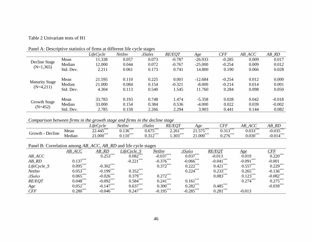
46

Table 2 Univariate tests of H1

Panel A: Descriptive statistics of firms at different life cycle stages LifeCycle NetInv ΔSales RE/EQT Age CFF AB_ACC AB_RD

Decline Stage

(N=1,365)

Mean 11.338 0.057 0.073 -0.787 -26.933 -0.285 0.009 0.017

Median 12.000 0.044 0.072 -0.767 -25.000 -0.254 0.009 0.012

Std. Dev. 2.211 0.061 0.173 0.741 14.800 0.190 0.066 0.028

Maturity Stage

(N=4,211)

Mean 21.595 0.110 0.225 0.001 -12.684 -0.254 0.012 0.000

Median 21.000 0.084 0.154 -0.321 -8.000 -0.214 0.014 0.001

Std. Dev. 4.304 0.113 0.540 1.545 11.760 0.284 0.098 0.050

Growth Stage

(N=452)

Mean 33.783 0.193 0.748 1.474 -5.358 0.028 0.042 -0.018

Median 33.000 0.154 0.384 0.536 -4.000 0.022 0.039 -0.002

Std. Dev. 2.785 0.158 2.266 2.294 3.903 0.441 0.144 0.082

Comparison between firms in the growth stage and firms in the decline stage LifeCycle NetInv ΔSales RE/EQT Age CFF AB_ACC AB_RD

Growth - Decline Mean 22.445

*** 0.136

*** 0.675

*** 2.261

*** 21.575

*** 0.313

*** 0.033

*** -0.035

***

Median 21.000***

0.110***

0.312***

1.303***

21.000***

0.276***

0.030***

-0.014***

Panel B: Correlation among AB_ACC, AB_RD and life cycle stages AB_ACC AB_RD LifeCycle_S NetInv ΔSales RE/EQT Age CFF

AB_ACC 0.253***

0.082***

-0.037***

0.037***

-0.013 0.019 0.220***

AB_RD 0.137***

-0.221***

-0.376***

-0.066***

-0.041***

-0.091***

-0.001

LifeCycle_S 0.095***

-0.302***

0.372***

0.222***

0.421***

0.557***

0.229***

NetInv 0.053***

-0.199***

0.352***

0.224***

0.233***

0.265***

-0.136***

ΔSales 0.065***

-0.026***

0.379***

0.272***

0.083***

0.123***

-0.082***

RE/EQT 0.048***

-0.092***

0.584***

0.241***

0.161***

0.274***

0.275***

Age 0.052***

-0.147***

0.637***

0.300***

0.282***

0.485***

-0.039***

CFF 0.280***

-0.046***

0.247***

-0.195***

-0.285***

0.281***

-0.013

47

Sample period: 1989 – 2004. Pearson (Spearman) correlations are presented above (below) the diagonal. ***

, **

and * represent significance at 1%, 5% and 10%,

respectively.


NetInv: capital expenditure (Compustat Data128) plus R&D expenditure (Data46) minus depreciation and amortization (Data14) scaled by beginning total assets

(Data6); ΔSales: growth in sales (Data12); RE/EQT: retained earnings (Data36) divided by total equity (Data60), multiplied by (-1); Age: the number of years the

firm first appears on either Compustat or CRSP, whichever is longer, multiplied by (-1); CFF: the difference between cash flow from financing activities

(Data311) and cash flow from operating activities (Data308), scaled by beginning total assets (Data6). AB_ACC: residual from the model of normal level of total

accruals; AB_RD: residual from the model of normal level of R&D expenditures, multiplied by -1. LifeCycle: the total ranks for NetInv, ΔSales, RE/EQT, Age,

and CFF. LifeCycle_S is defined as LifeCycle scaled by 45.

48


Panel A: Descriptive statistics of firms with different levels of stock-based compensation sensitivity to stock price INC_RATIO_RANK = 1 (Smallest), N = 684

AB_ACC AB_RD INC_RATIO OPT_GNT OPT_UNE OPT_EXE RST_GNT STK_OWN

Mean 0.003 -0.002 0.027 0.170 0.595 0.943 0.055 0.225

Median 0.007 -0.001 0.029 0.097 0.427 0.599 0.000 0.114

Std. Dev. 0.084 0.029 0.015 0.244 0.817 1.043 0.391 0.414

INC_RATIO_RANK = 2 , N = 684


Mean 0.008 -0.006 0.077 0.252 0.549 0.807 0.039 0.454

Median 0.010 -0.004 0.074 0.170 0.387 0.559 0.000 0.221

Std. Dev. 0.080 0.034 0.016 0.291 0.579 0.945 0.102 0.701

INC_RATIO_RANK = 3 , N = 685


Mean 0.006 -0.007 0.172 0.334 0.622 0.881 0.036 1.360

Median 0.011 -0.003 0.162 0.171 0.419 0.512 0.000 0.540

Std. Dev. 0.082 0.040 0.047 0.533 0.678 1.174 0.234 2.526

INC_RATIO_RANK = 4 (Largest) , N = 684


Mean 0.011 -0.012 0.594 0.274 0.529 0.804 0.033 8.365

Median 0.009 -0.004 0.586 0.085 0.285 0.347 0.000 4.736

Std. Dev. 0.081 0.043 0.212 0.536 0.787 1.437 0.326 9.409

Difference b/w firms with the largest INC_RATIO and the smallest INC_RATIO


Mean 0.008*

-0.010***

0.567***

0.104***

-0.066 -0.139**

-0.022 8.140***

Median 0.002 -0.003***

0.557***

-0.012 -0.142***

-0.252***

0.000***

4.622***

49

Panel B: Correlation among AB_ACC, AB_RD and stock-based compensation incentives AB_ACC ABN_RD INC_RATIO OPT_GNT OPT_UNE OPT_EXE RST_GNT STK_OWN

AB_ACC -0.279***

0.039**

-0.089***

-0.002 0.021 -0.012 0.066***

AB_RD -0.169***

-0.100***

0.043**

0.037 0.034 0.007 -0.053***

INC_RATIO 0.030 -0.113***

0.011 -0.062***

-0.075***

-0.036 0.647***

OPT_GNT -0.015 0.067***

0.023 0.620***

0.282***

0.013 -0.023

OPT_UNE 0.005 0.064***

-0.103***

0.627***

0.336***

0.057***

-0.037

OPT_EXE 0.017 0.093***

-0.151***

0.337***

0.445***

0.008 -0.019

RST_GNT -0.014 -0.004 -0.139***

-0.028 -0.020 -0.056***

-0.024

STK_OWN 0.045**

-0.007 0.661***

-0.042**

-0.015 0.090***

-0.105***

Number of observations: 2,737. Sample period: 1992-2004. Pearson (Spearman) correlations are presented above (below) the diagonal. ***

, **

and * represent

significance at 1%, 5% and 10%, respectively.


AB_ACC: residual from the model of normal level of total accruals; AB_RD: residual from the model of normal level of R&D expenditures, multiplied by -1.

INC_RATIO: constructed as ONEPCT / (ONEPCT + SALARY + BONUS). ONEPCT is the dollar change in the value of CEO stock and option holdings coming

from a one percent increase in the firm’s stock price. OPT_GNT: option grants scaled by total outstanding shares of the firm, multiplied by 100; OPT_UNE:

unexercisable options (excluding option grants) scaled by total outstanding shares of the firm, multiplied by 100; OPT_EXE: exercisable options scaled by total

outstanding shares of the firm, multiplied by 100; RST_GNT: restricted stock grants scaled by total outstanding shares of the firm, multiplied by 100; STK_OWN:

total shares held by the manager scaled by total outstanding shares of the firm, multiplied by 100.

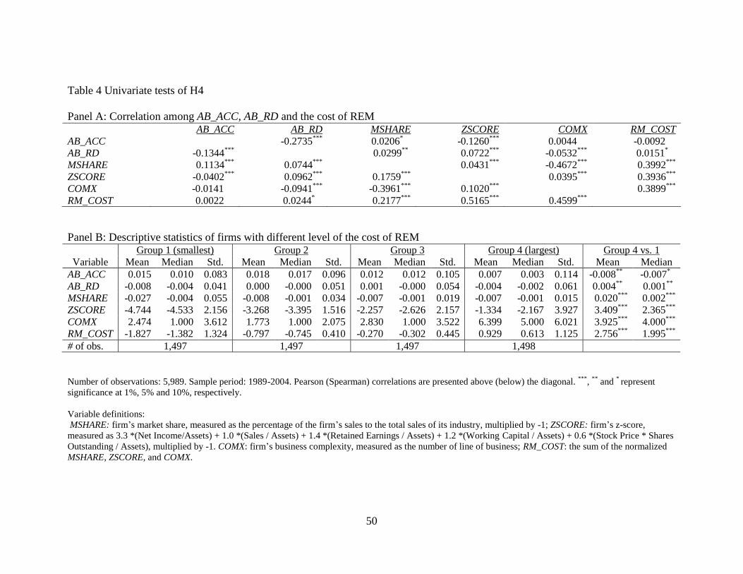
50


Panel A: Correlation among AB_ACC, AB_RD and the cost of REM AB_ACC AB_RD MSHARE ZSCORE COMX RM_COST

AB_ACC -0.2735***

0.0206*

-0.1260***

0.0044 -0.0092

AB_RD -0.1344***

0.0299**

0.0722***

-0.0532***

0.0151*

MSHARE 0.1134***

0.0744***

0.0431***

-0.4672***

0.3992***

ZSCORE -0.0402***

0.0962***

0.1759***

0.0395***

0.3936***

COMX -0.0141 -0.0941***

-0.3961***

0.1020***

0.3899***

RM_COST 0.0022 0.0244*

0.2177***

0.5165***

0.4599***

Panel B: Descriptive statistics of firms with different level of the cost of REM Group 1 (smallest) Group 2 Group 3 Group 4 (largest) Group 4 vs. 1

Variable Mean Median Std. Mean Median Std. Mean Median Std. Mean Median Std. Mean Median

AB_ACC 0.015 0.010 0.083 0.018 0.017 0.096 0.012 0.012 0.105 0.007 0.003 0.114 -0.008**

-0.007*

AB_RD -0.008 -0.004 0.041 0.000 -0.000 0.051 0.001 -0.000 0.054 -0.004 -0.002 0.061 0.004**

0.001**

MSHARE -0.027 -0.004 0.055 -0.008 -0.001 0.034 -0.007 -0.001 0.019 -0.007 -0.001 0.015 0.020***

0.002***

ZSCORE -4.744 -4.533 2.156 -3.268 -3.395 1.516 -2.257 -2.626 2.157 -1.334 -2.167 3.927 3.409***

2.365***

COMX 2.474 1.000 3.612 1.773 1.000 2.075 2.830 1.000 3.522 6.399 5.000 6.021 3.925***

4.000***

RM_COST -1.827 -1.382 1.324 -0.797 -0.745 0.410 -0.270 -0.302 0.445 0.929 0.613 1.125 2.756***

1.995***

# of obs. 1,497 1,497 1,497 1,498

Number of observations: 5,989. Sample period: 1989-2004. Pearson (Spearman) correlations are presented above (below) the diagonal. ***

, **

and * represent

significance at 1%, 5% and 10%, respectively.


MSHARE: firm’s market share, measured as the percentage of the firm’s sales to the total sales of its industry, multiplied by -1; ZSCORE: firm’s z-score,

measured as 3.3 *(Net Income/Assets) + 1.0 *(Sales / Assets) + 1.4 *(Retained Earnings / Assets) + 1.2 *(Working Capital / Assets) + 0.6 *(Stock Price * Shares

Outstanding / Assets), multiplied by -1. COMX: firm’s business complexity, measured as the number of line of business; RM_COST: the sum of the normalized

MSHARE, ZSCORE, and COMX.

51

Table 5: Regression analyses

AB_ACCt = β0 + β1 AB_RDt + β2 LIFECYCLE_St + β3 INC_RATIOt + β4 LAGPEt

+ β5 RM_COSTt + β6 NOAt + β7 BIG8t + β8 LEVt + β9ROAt +Year Controls

+ Industry Controls + εt

AB_RDt = γ0 + γ1 LIFECYCLE_St + γ2 INC_RATIOt + γ3 LAGPEt + γ4 RM_COSTt

+ γ5 NOAt + γ6 BIG8t + γ7 LEVt + γ8 ROAt +Year Controls

+ Industry Controls + εt

AB_ACC AB_RD

Pred. Sign Coeff. p value Pred. Sign Coeff. p value

Intercept ? 0.0206 0.1793 ? -0.0191 0.0004

AB_RD ? 0.6404 0.0000

LIFECYCLE_S + 0.0533 0.0000 - -0.0583 0.0000

INC_RATIO + 0.0175 0.0042 - -0.0085 0.0003

LAGPE + 0.0003 0.0020 - -0.0000 0.0263

RM_COST - -0.0026 0.0119 + -0.0002 0.3076

NOA - 0.0009 0.4246 + -0.0096 0.0000

BIG8 - -0.0227 0.0200 + 0.0110 0.0023

LEV ? 0.0000 0.9949 ? 0.0003 0.5267

ROA ? 0.0103 0.6949 ? -0.0600 0.0000

SIZE ? -0.0016 0.1981 ? -0.0007 0.0856

Year Dummies YES YES

Ind. Dummies YES YES

Adj. R2

7.35% 15.57%

Number of observations: 1,834. Sample period 1992 to 2004.

T-statistics are based on Newey and West’s (1987) heteroscedasticity and autocorrelation consistent

standard error estimates. All p values are based on one-tailed t tests when the coefficient sign is predicted,

and based on two-tailed t tests otherwise.


AB_ACC: residual from the model of normal level of total accruals; AB_RD: residual from the model of

normal level of R&D expenditures, multiplied by -1. INC_RATIO: constructed as ONEPCT / (ONEPCT +

SALARY + BONUS). LifeCycle_S : defined as LifeCycle scaled by 45, where LifeCycle is the total ranks for

NetInv, ΔSales, RE/EQT, Age, and CFF. LAGPE: price to earnings ratio at the beginning of the period.

RM_COST: the sum of the normalized MSHARE, ZSCORE, and COMX. NOA: lagged net operating assets

scaled by sales. BIG8: 1 if the firm is audited by a Big 8 auditor; 0 otherwise. LEV: debt/equity. ROA:

return on assets. SIZE: log of market value of equity.

52

Table 6 Regression analysis using individual components of RM_COST

Panel A Dependent variable = AB_ACC Model 1 Model 2 Model 3 Model 4

Pred.

Sign

Coeff. p value Coeff. p value Coeff. p value Coeff. p value

Intercept ? 0.0273 0.0763 0.0420 0.0062 0.0279 0.0565 0.0314 0.0483

AB_RD ? 0.6355 0.0000 0.6569 0.0000 0.6463 0.0001 0.6594 0.0000

LIFECYCLE_S + 0.0479 0.0002 0.0489 0.0002 0.0573 0.0000 0.0585 0.0000

INC_RATIO + 0.0163 0.0064 0.0218 0.0007 0.0198 0.0013 0.0238 0.0003

LAGPE + 0.0002 0.0018 0.0004 0.0003 0.0004 0.0006 0.0004 0.0011

MSHARE - -0.0179 0.3060 -0.0956 0.0165

ZSCORE - -0.0056 0.0005 -0.0050 0.0016

SID - -0.0012 0.0000 -0.0011 0.0009

NOA - 0.0043 0.3284 -0.0058 0.2546 0.0026 0.5538 -0.0058 0.2582

BIG8 - -0.0223 0.0215 -0.0223 0.0218 -0.0237 0.0165 -0.0232 0.0177

LEV ? 0.0001 0.9347 -0.0004 0.7663 -0.0001 0.9402 -0.0003 0.8329

ROA ? 0.0011 0.9654 0.0726 0.0317 0.0239 0.3638 0.0737 0.0301

SIZE ? -0.0026 0.0453 -0.0024 0.0286 -0.0042 0.0004 -0.0020 0.1493

Year Dummies YES YES YES YES

Industry Dummies YES YES YES YES

Adj. R2

7.05% 7.58% 7.88% 8.15%

53

Panel B Dependent variable = AB_RD Model 1 Model 2 Model 3 Model 4

Pred.

Sign

Coeff. p value Coeff. p value Coeff. p value Coeff. p value

Intercept ? 0.0186 0.0007 0.0162 0.0033 0.0209 0.0000 0.0156 0.0064

LIFECYCLE_S - -0.0606 0.0000 -0.0611 0.0000 -0.0626 0.0000 -0.0617 0.0000

INC_RATIO - -0.0100 0.0000 -0.0081 0.0005 -0.0096 0.0000 -0.0079 0.0007

LAGPE - -0.0001 0.1492 -0.0000 0.2884 -0.0001 0.1298 -0.0000 0.3250

MSHARE + 0.0214 0.0458 0.0081 0.6174

ZSCORE + -0.0018 0.0014 -0.0017 0.0054

SID + 0.0002 0.0250 0.0001 0.3913

NOA + 0.0102 0.0001 0.0132 0.0000 0.0103 0.0000 0.0130 0.0000

BIG8 + -0.0116 0.0035 -0.0115 0.0038 -0.0114 0.0041 -0.0114 0.0043

LEV ? -0.0003 0.5348 -0.0002 0.7198 -0.0003 0.5015 -0.0001 0.7669

ROA ? 0.0543 0.0000 0.0323 0.0070 0.0530 0.0001 0.0312 0.0108

SIZE ? 0.0011 0.0230 0.0006 0.1066 0.0009 0.0259 0.0009 0.0707

Year Dummies YES YES YES YES

Industry Dummies YES YES YES YES

Adj. R2

16.23% 16.63% 16.27% 16.58%

Number of observations: 1,834. Sample period 1992 to 2004.

T-statistics are based on Newey and West’s (1987) heteroscedasticity and autocorrelation consistent standard error estimates. All p values are based on one-tailed

t tests when the coefficient sign is predicted, and based on two-tailed t tests otherwise.


MSHARE: firm’s market share, measured as the percentage of the firm’s sales to the total sales of its industry, multiplied by -1; ZSCORE: firm’s z-score,

measured as 3.3 *(Net Income/Assets) + 1.0 *(Sales / Assets) + 1.4 *(Retained Earnings / Assets) + 1.2 *(Working Capital / Assets) + 0.6 *(Stock Price * Shares

Outstanding / Assets), multiplied by -1. COMX: firm’s business complexity, measured as the number of line of business; See Table 5 for definitions of other

variables.

the choice between real and accounting earnings …the choice between real and accounting earnings...

Documents