the causes and consequences of inequality: land
TRANSCRIPT

THE CAUSES AND CONSEQUENCES OF INEQUALITY: LAND DISTRIBUTION, DIVERSITY, AND SOCIAL OUTCOMES
Andrew Stephen Pennock
A dissertation submitted to the faculty of the University of North Carolina at Chapel Hill in partial fulfillment of the requirements for the degree of Doctor of Philosophy in the Department of Political Science.
Chapel Hill 2011
Approved by:
Thomas Oatley
John Stephens
Timothy McKeown
Mark Creczenzi
Stephen Gent

ii
©2011 Andrew Stephen Pennock
ALL RIGHTS RESERVED

iii
ABSTRACT
ANDREW PENNOCK: The Causes and Consequences of Inequality: Land Distribution, Diversity, and Social Outcomes
(Under the direction of Thomas Oatley)
Understanding the organizational ability of groups in society is essential to
understanding political outcomes. Land distribution and ethnic diversity both affect the
ability of groups to organize effectively and influence policy. Using a three-article format, I
employ a newly released land inequality dataset to show that powerful landowners are able to
influence education attainment, that ethnic diversity has a strong, negative cross-national
effect on social spending, and large landowners have a moderating effect on economic
inequality during industrialization.

iv
DEDICATION
For my wife, Charity, who believed in me and supported me through the process of
writing this. Thanks for helping me realize my dream of becoming a professor.

v
ACKNOWLEDGEMENTS
I owe a great many debts of thanks for the completion of this dissertation.
Foremost among them is the debt owed to Thomas Oatley who patiently reviewed the
manuscript at every stage of the process. His insightful questions, steady guidance,
mentorship, and faith in my ability to complete this project made it possible. I am grateful
to my other committee members, Mark Creczenzi, Tim McKeown, and John Stephens, for
their considerable feedback on both the proposal and the completed manuscript. I am
grateful to each of them for their mentorship in the profession. They are exemplar teachers,
scholars, and mentors. I am very blessed to have a committee comprised of professors
whom I admire as people as well as scholars. Finally, while François Nielsen’s name does
not appear on the title page because of illness, I am grateful to him for his input on this
project, especially on the third chapter. I am also grateful to Stephen Gent for joining the
committee in his stead.
Two graduate student colleagues have been pillars of support through this process.
Erik Godwin is as faithful a friend as I have known. Without his friendship and his
encouragement to believe I could succeed as a professional this project would not have
come to fruition. Christine Carpino has been a constant and wonderful encouragement.
Both encouraged me through the lowest and highest points of the process and read many
drafts. Many other graduate student colleagues have comprised the social fabric that makes
graduate school more enjoyable. I am thankful for their friendship, especially Sarah Bauerle,
Russell Bither-Terry, Tim Cupery, Chris Dittmeier, Matt Harper, Katja Kleinberg, and
Jessica Meed. Finally, I am particularly grateful to the staff in the department, Chris

vi
Reynolds, Shannon Eubanks, and Carol Nichols, for their help and support in ways both
small and great.
Two professors from Clemson University inspired me to become an academic. Dr.
J. David Woodard taught me to love the study of politics. Dr. Lee Morrissey is the teacher I
try to be in the classroom. I am grateful to them both.
Success in graduate school depends as much on support outside of the university as
within it. I have been blessed beyond reason in this arena. Grace Community Church has
been my spiritual and emotional home since my first weeks in Chapel Hill. Bill, Valerie, Finn
and Colin Cooley took me in as family when I needed it the most. The friendship of Steve,
Jeannie, Anna, and Kaelen Cox means more to me than words can express. Bret Horton,
Tim Marshall, Bart Dunlap, and Ben Sammons have offered many prayers in hopes of seeing
this document completed. Finally, Dr. David Stotts bridged the gap between church and
work. He gave freely of his time and talents to a graduate student outside of his department.
I am grateful. The broader church community has supported my wife, Charity, and me with
prayers, food, tears, and laughter. Thank you.
Another gift beyond reason has been the support and friendship of the Sommerfeld
family. Dr. Roy and Emma Sommerfeld were a favorite part of my life here before their
passing. I do not know what these years would have been like without the Sommerfelds and
the life Charity and I have lived in their home, garden, and lives. All I know is that I am
grateful beyond the ability to repay to Doc, Emma, Marti, Tom, Elinore, and Pete. Pete
visited me more in Chapel Hill than any other person and I now count him as a fast friend.
I came to graduate school with great family support and leave with everyone
celebrating. My parents, Steve and Helen Pennock, equipped me with the curiosity, faith,
and skills to succeed as a professor. Thank you for nurturing me and supporting my dream.

vii
My sisters, Elizabeth and Katie (both of whom are brighter than me), have always
encouraged me through this process. My grandparents, Charles and Lillian Kendrick have
probably offered more prayers for my success than I have. Dr. JoAnn Nishimoto and her
husband, Stuart Nishimoto, have been vocal cheerleaders. My biggest support is, of course,
my wife Charity. As wonderful as she is as a copy editor, she is a better partner in life. I am
grateful.
Finally, I am grateful to God for his faithfulness to me in this season of my life. My
experience at UNC has been filled with more blessings than I could have dreamed, both
professionally and personally. To God be the glory.

viii
TABLE OF CONTENTS
LIST OF TABLES............................................................................................................................... x
LIST OF FIGURES .......................................................................................................................... xi
Chapter
I. THE POLITICS OF DOMESTIC LABOR MOBILITY.......................................1
Introduction......................................................................................................................1
Specific Factors and the Incentive for Political Control of Labor Mobility...........4
Empirical Analysis………………................................................................................9
Methods and Results.....................................................................................................15
Conclusion......................................................................................................................19
II. DIVERSITY AND SOCIAL SPENDING..............................................................27
Introduction....................................................................................................................27
Diversity and Social Spending......................................................................................27
Empirical Analysis.........................................................................................................32
Methods and Results.....................................................................................................40
Conclusion......................................................................................................................45
III. EXPLAINING INCOME INEQUALITY ............................................................54
Introduction....................................................................................................................54
Literature Review...........................................................................................................55
Theory..............................................................................................................................57 Data..................................................................................................................................59

ix
Methods...........................................................................................................................62 Analysis and Results......................................................................................................62
Conclusion......................................................................................................................68
APPENDICES ...................................................................................................................................77 REFERENCES...................................................................................................................................86
x
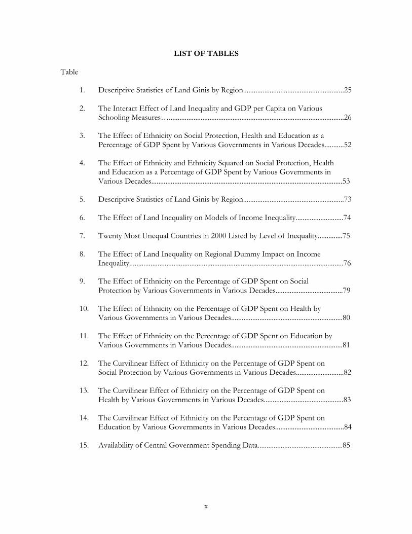
LIST OF TABLES
Table
1. Descriptive Statistics of Land Ginis by Region.........................................................25
2. The Interact Effect of Land Inequality and GDP per Capita on Various Schooling Measures…...................................................................................................26
3. The Effect of Ethnicity on Social Protection, Health and Education as a
Percentage of GDP Spent by Various Governments in Various Decades...........52
4. The Effect of Ethnicity and Ethnicity Squared on Social Protection, Health and Education as a Percentage of GDP Spent by Various Governments in Various Decades............................................................................................................53
5. Descriptive Statistics of Land Ginis by Region.........................................................73
6. The Effect of Land Inequality on Models of Income Inequality...........................74
7. Twenty Most Unequal Countries in 2000 Listed by Level of Inequality..............75
8. The Effect of Land Inequality on Regional Dummy Impact on Income
Inequality.........................................................................................................................76
9. The Effect of Ethnicity on the Percentage of GDP Spent on Social Protection by Various Governments in Various Decades......................................79
10. The Effect of Ethnicity on the Percentage of GDP Spent on Health by
Various Governments in Various Decades...............................................................80
11. The Effect of Ethnicity on the Percentage of GDP Spent on Education by Various Governments in Various Decades...............................................................81
12. The Curvilinear Effect of Ethnicity on the Percentage of GDP Spent on Social Protection by Various Governments in Various Decades...........................82
13. The Curvilinear Effect of Ethnicity on the Percentage of GDP Spent on
Health by Various Governments in Various Decades.............................................83
14. The Curvilinear Effect of Ethnicity on the Percentage of GDP Spent on Education by Various Governments in Various Decades.......................................84
15. Availability of Central Government Spending Data................................................85

xi
LIST OF FIGURES
Figures
1. Land Inequality and Percentage of the Over-15 Population with Some Secondary Education in Countries with GDP per Capita Incomes Above the Median in 1980...............................................................................................................22
2. Land Inequality and Percentage of the Over-15 Population with Some Secondary Education in Countries with GDP per Capita Incomes Below the Median in 1980...............................................................................................................22
3. Marginal Effect of Land Inequality on the % of Population that are Secondary
School Graduates as GDP per Capita Changes........................................................23
4. Marginal Effect of Land Inequality on % of Population that are Primary School Graduates as GDP per Capita Changes........................................................23
5. Marginal Effect of Land Inequality on Any Schooling as GDP per Capita
Changes...........................................................................................................................24
6. Marginal Effect of Land Inequality on Average Years of Schooling as GDP per Capita Changes........................................................................................................24
7. Box Plot of Ethnic Diversity Scores by Regions......................................................47
8. Average Percentage of GDP spent on Social Spending vs. Ethnic Diversity in
the OECD during 1980s...............................................................................................47
9. Average Percentage of GDP spent on Social Spending vs. Ethnic Diversity during 1980s....................................................................................................................48
10. Health Spending in Canada 2001-2007 in Thousands of Canadian Dollars by
Central & State Governments......................................................................................48
11. Health Spending in Germany 2001-2007 in Thousands of Euros.........................49
12. Central Government Healthcare Spending in Israel 1995-2005 in Thousands of National Currency.....................................................................................................49
13. Central Government Healthcare Spending in Finland 1990-2005 in Thousands
of National Currency.....................................................................................................50
14. Central Government Healthcare Spending in the Netherlands 1990-2007 in Thousands of National Currency................................................................................50
15. Ethnic Diversity Scores of Countries Reporting Social Spending Data vs.
Those Not Reporting....................................................................................................51

xii
16. Curvilinear Effect of Ethnicity on Social Spending in Model 7.............................51
17. Kuznets Curve by Land Inequality Level...................................................................70
18. Income Inequality by Region in 2000.........................................................................71
19. Land Inequality by Region in 2000.............................................................................71
20. Latin American Influence on the Relationship between Income Inequality and
Land Inequality...............................................................................................................72

CHAPTER 1
THE POLITICS OF DOMESTIC LABOR MOBILITY: SPECIFIC FACTORS, LANDOWNERS, AND EDUCATION
Introduction
For the first 350 years of European colonization, New World governments divided
domestic labor markets into two groups, slaves and freemen. Freemen responded to market
pressures for their laborers and received market wages while slaves worked as unpaid, forced
labor bound to their owner’s land. Landowners reaped the benefits of this system by
undercutting agricultural competitors around the world who had to pay their laborers wages.
Gradually, violent and non-violent events in the New and Old Worlds brought an end to
slavery. Slaves became freemen, joined national labor forces, and began competing for jobs
off the farm as well as on it. The abolition of slavery created a national labor pool and a
functioning labor market free from political intervention.
The abolition of slavery did not, however, end the economic incentives of
landowners to keep agricultural workers from leaving their farms. Landowners lost the
battle over legalized slavery at the national level and so turned to other tactics to capture
laborers, keep wages low, and maintain their profits. One prominent method of achieving
this was to deny rural workers education because uneducated workers had a difficult time
leaving farms and finding employment elsewhere. 1 If landowners could prevent their
workers from becoming educated could also keep them on the farm. The battle over
laborers’ ability to move from one type of employment to another therefore shifted from
1 Cohen (1991) and Blackmon (2008) discuss other methods landowners in the United States used to keep labor from migrating, including intimidation and mass imprisonment.

2
national battles over slavery to local and state battles over education. Here powerful
landowners could still successfully use their political influence to limit labor mobility by
limiting education. Occasionally this battle involved national players but for the most part
education policy was and is made at the state and local level where landowners were
particularly powerful.2
This neglected story of landowner influence on education is important for today’s
students of domestic labor mobility, many of who are political economists. Labor mobility
plays a key role determining how political conflict is organized in society. For example, trade
politics are alternately characterized as a conflict between the factors of production (capital,
labor, and land) when labor mobility is high or a conflict between sectors (i.e. specific
industries) when labor mobility is low. Because labor mobility predicts when either model is
appropriate, scholars have spent considerable time and effort measuring labor mobility
(Hiscox 2001)(Hiscox 2002)(Ladewig 2006)(Mukherjee, Smith, and Li 2009). These studies
strengthened our empirical knowledge of how labor mobility has changed over time and, in
turn, improved our understanding of why political coalitions form in response to economic
conflict.
While a great deal of attention has been paid to the political influences of labor
mobility very little attention has been paid to the political influences on labor mobility.
Understanding which political actors influence labor mobility and why they do so is
important because it may be the case that labor markets are not as free of political influence
as our models assume. Standard political models begin by assuming that labor mobility is
technologically determined. This is a useful assumption for model building, but a strange
2 For example, the Civil Rights movement involved the federal government in the battle over state and local school desegregation. After this brief period of national exposure the politics of education and labor mobility largely disappeared from the national political debate, and landowners in the rural South to try to control rural worker’s ability to migrate out of rural areas.

3
one for political economists to make. Labor mobility is heavily influenced by education, a
public good generally provided by governments. And like any government policy, education
is subject to political battles by interested parties. Political actors battle over labor mobility
today, just as they have for centuries. In the late 20th and early 21st century labor has been
largely (but sadly not entirely) free from the explicit restrictions on labor mobility that have
been employed in the past (slavery, serfdom, and migration restrictions). The battle
continues, but now occurs over education policy.
This paper argues that actors within the national political system continue to
influence education specifically to influence labor mobility. Education is a key determinant
of labor mobility and political actors recognize this. In countries with industrial labor
markets, agricultural landowners attempt to restrict education, resulting in limited labor
mobility, a higher supply of rural workers, and depressed agricultural wages. Conversely, in
countries without competing industrial labor markets agricultural landowners need not worry
about the mobility of their laborers. These landowners have an incentive to provide some
education to improve the productivity of their workers. In either case, when agricultural
actors are powerful enough, they are dramatically successful in altering educational outcomes
to achieve their ends.
I establish this political dynamic using a specific-factors model to show the economic
motivations of landowners with respect to education in the national economy. Then, I show
that land inequality is an indicator of the political power of landowners and their ability to
achieve their political ends. I present evidence demonstrating a conditional relationship
between land inequality and educational outcomes that is consistent with the predictions of
the specific-factors model. I conclude by reflecting on how these findings affect our broader
understanding of national and international politics.

4
Specific Factors and the Incentive for Political Control of Labor Mobility
Landowners are concerned about their workers’ education levels because it affects
worker mobility and worker productivity. Education affects labor mobility, the ability of
workers to change jobs, in both developed and developing countries (Sjaastad
1962)(Greenwood 1971)(1975) . Despite the clear economic interest that landowners have in
education, many political models treat education as structurally determined. Labor mobility
is therefore assumed to be structurally determined as well, usually by exogenous
technological change. For example, Hiscox (2002) documents changes in labor mobility
over the course of industrialization. His research shows that labor mobility is high in the
early stages of industrialization. The rise of urban industries created a huge need for low-
skilled laborers to work in urban settings. Their high productivity produced high wages,
increased income inequality, and encouraged rural to urban migration. Because neither
agricultural nor industrial labor are assumed to be particularly skilled, laborers can migrate
between rural and urban areas, forming a national labor pool. Migration is aided by the
emergence of national education, communication, and transportation systems that allow
rural workers to learn of new opportunities, give them the skills to work in these new jobs,
and give workers the ability to travel to them with increasing ease. However, as
industrialization continues, labor gradually becomes less mobile. New methods of
production require specialized training. Workers are no longer able to move between jobs
with the same ease as before.
This change from mobile to immobile labor has two effects. First, it effectively
divides the national labor pool into urban and rural labor pools. Second, it divides urban
labor by industrial sector. A typical urban worker is now unable to quit his or her job in
garment manufacturing to work in the steel mill, the two skill sets are simply too different to

5
make an easy transition possible. Hiscox uses the historical development of labor mobility
as his point of departure for examining the dynamics of trade coalition formation. It is a
compelling story, and one that assumes politics does not influence labor mobility.
A specific-factors model shows why groups in society have an incentive to influence
labor mobility.3 Each country is assumed to be a closed labor market. There are two sectors
in the country, agriculture and manufacturing, both of which require the input of two factors
to produce their products. Agriculture requires inputs of land and of labor. Manufacturing
requires inputs of capital and of labor. Land and capital are fixed factors, meaning that they
can only be used to produce goods in agriculture and industry respectively. Labor is the
mobile factor, meaning that laborers are assumed to move from one sector to the other
based on demand. Wages are determined by the interaction of labor demand between the
manufacturing and agricultural sector. The specific-factors model assumes diminishing
returns to labor in both sectors. Because each additional worker per sector is slightly less
productive than the previous one, there is a point at which employers cease to hire new
employees because they would produce less value than the wage they would be paid. In the
model, the wages paid by each sector are the same because an imbalance in wages causes
labor to migrate from the low paying sector to the high paying sector.
Now assume a productivity shock significantly improves the marginal productivity of
labor in manufacturing. This shock throws the system out of equilibrium. The total demand
for labor in manufacturing increases and manufacturers now try to employ additional
laborers. Wages in the manufacturing sector increase because there is the same supply of
manufacturing workers and a higher demand for them. Manufacturers compete amongst
3 The specific-factors model makes a number of assumptions which if violated will impinge on the predictive abilities of the model. If the owners of land are also the owners of capital then society is best described by a factor, not a specific-factors, model. In such a society owners are not incentivized to control the flow of labor between factors because they set wages in both of them.

6
themselves to employ a fixed number of industrial laborers. Because the supply of industrial
workers is fixed, the workers’ wages rise. The workers, not the manufacturers, profit from
the increase in productivity as their wages rise. Meanwhile the agricultural sector is
unaffected. The supply and demand for agricultural laborers remains constant so wages
remain constant as well.
In the long-run, however, the productivity shock in manufacturing alters the labor
supply and the wages paid in the agricultural sector as well. Labor shifts from agricultural
employment to industrial employment in response to higher wages offered in the
manufacturing sector. This causes the number of laborers in the agriculture to shrink. A
smaller supply of labor and constant demand for it results in higher wages. Wages for both
factors equilibrate and labor stops migrating. Industrial wages are now lower than they were
immediately after the shock, but higher than they were before the shock occurred.
Conversely, agricultural wages are now higher. Assuming that the international market sets
prices for the goods produced by both sectors, then the following distributional
consequences occur: the manufacturers have higher profits; laborers in both manufacturing
and agriculture have higher wages. Only the landowners lose. Their profits decline because
they must now pay higher wages to their laborers while selling their goods at the same price
as before.
Politics enters the specific-factors model when the degree of labor mobility can be
influenced by political actions. In the example above, the productivity shock decreased the
number of workers in agriculture. Any decrease in the supply of rural labor will result in
rising wages paid by agricultural landowners. Unless landowners can prevent labor from
migrating and wages from equilibrating they are trapped between the new price of their labor
and the fixed prices their goods fetch on the international market. Therefore in a specific-

7
factor framework, factor owners have a strong incentive to create policies that restrict or
enhance labor mobility.
Agricultural landowners restrict labor mobility by using their political influence to
prevent or slow labor migration to the cities.4 Though explicit labor restrictions are rare in
modern societies, education is a less explicit but still potent means of influencing labor
mobility. Economists have long linked education with an increased likelihood of labor
migration in both developed and developing countries (Sjaastad 1962)(Greenwood
1971)(Greenwood 1975)(Zhao 1997). Workers with higher levels of education are more
mobile. They are able to work in higher paid jobs and are more likely to migrate to cities.
Agricultural elites therefore have an incentive keep education levels low in order to keep
laborers in their labor pool.
Economic interest does not perfectly translate into political influence. The more
politically powerful landowners are as a group, the greater their ability to affect education
levels.5 Like any group, landowners are better able to realize their interest when they are able
to overcome the collective action problem effectively for their preferences (Olson 1965).
Agriculture elites should therefore be successful when land is concentrated in the hands of
the few. A relatively small group of landowners will accrue the benefits of reduced labor
mobility instead of the benefits being spread over thousands or hundreds of thousands of
4 Both fixed-factors, agriculture and industry, have an incentive to influence labor mobility. Urban industries have a difficult time influencing rural education because education policy is primarily made at the state and local level. Similarly, agricultural and industrial laborers have competing goals with respect to labor mobility. Agricultural labors want more mobility so they can move to jobs with higher wages. Industrial workers use their power to restrict labor mobility of rural workers by creating insider-outsider politics (Rueda 2005)(2007). 5 Powerful landowners have also played a pivotal role in democratization (Moore 1966)(Rueschemeyer, E. Stephens, and J. D. Stephens 1992)(Huber and Safford 1995)(Acemoglu and Robinson 2000)(2006b)(2006a) and trade policy (Gerschenkron 1943).
8
landowners.6 The concentrated benefits of lower wages incentivize the large landowners to
take political action. Their small numbers increase their ability to sanction free riders that
shirk the costly lobbying efforts required to keep education levels low. Thus, concentrated
landowning enables landowners to overcome the collective action problem and decrease
educational provision.7 This reduces labor mobility and keeps income inequality high. This
theoretical expectation is in line with previous case study and large-N work relating land
inequality to education (Banerjee and Iyer 2005)(Galor, Moav, and Vollrath 2009)(Wegenast
2009)(2010).
Countries with high levels of economic development display exactly this dynamic as
Figure 1 indicates. Figure 1 plots the relationship between education (represented as the
percentage of the population over age 15 that has some secondary schooling) and land
inequality for countries with GDP-per-capita incomes above the median in 1980. As shown
in this figure, land inequality is negatively correlated with education.8 The higher the land
inequality score, the lower the percentage of the over-15 population that has some secondary
education. This relationship supports the theory that landowners fear urban migration and
reduce education when they are politically able to do so.
The specific-factors model leads us to a different expectation in undeveloped
countries where landowners face a different calculus. Education increases productivity
6 This paper treats land inequality as an exogenous variable, but there is an interesting literature examining the origins of land inequality. Engerman and Sokoloff (2000)(2002) argue that modern land inequality in the Americas originates from factor endowments of particular soils and climates. For example, specific combinations of hot climates, rich soils and high rainfalls enabled large and very profitable sugar plantations in the Caribbean. Because the returns to scale are very high in sugar production, highly unequal landholding patterns emerged. See Easterly (2007) for an empirically test of this hypothesis and van de Walle (2009) for an extension to the African context. 7 Bates (1981) shows this same dynamic in the African context by studying the effectiveness of farmers in lobbying against price controls. 8 The strongest predictor of educational attainment is the level of development as discussed in the review of the control variables in the next section.

9
allowing more goods to be produced with the same quantities of labor and land. In
countries without an industrial sector, educated workers cannot migrate to better paying
industrial jobs because they simply do not exist. The agricultural labor pool remains the
same size and wages remain constant. Higher productivity and constant wages result in
higher profits for landowners. In this scenario, the productivity gains of education accrue
entirely to landowners. Education becomes a private good, solely benefiting the landowners,
instead of a public good benefiting society. Therefore in undeveloped societies, landowners
prefer more education because the productivity gains of education enrich the landowners.
High landowning inequality in poor countries empowers landowners to achieve their
educational goals as shown in Figure 2. Figure 2 plots the relationship between education
and land inequality in countries with GDP per Capita below the median in 1980. As
predicted, there is a positive relationship between land inequality and education.
Land inequality is positively correlated with the educational outcomes that
agricultural elites pursue in both rich and poor countries. The same high levels of land
inequality politically empower landowners to provide education in undeveloped countries
and deny education in developed ones. Developed societies with high levels of land
inequality have lower levels of education than those with low levels of land inequality. Less
developed societies with high levels of land inequality have higher levels of education than
those with low levels of land inequality. The theory and evidence lead to the expectation of
a conditional relationship between education and land inequality.
Empirical Analysis
Having established the theoretical reasons to expect a conditional relationship
between landownership patterns and education, I test for landowner influence on education
using a large-N analysis with educational attainment as my dependent variable. Because the

10
dependent variables are sampled at five-year intervals, all of the measures are collapsed into
five-year-averages
The dependent variable is education, which provides workers with skills and
increases their ability to migrate from rural to urban jobs. Barro and Lee (1996)(2001)
provide educational attainment figures for the over-15 population in 142 countries at five-
year intervals from 1960-2000. They measure the percentage of the population achieving
various levels of education. I run the model using four different measures of educational
attainment: percentage of the population that has graduated from secondary school,
percentage of the population that has graduated from primary school, percentage of the
population that has attended at least one year of school, and the average level of education.
Unfortunately, these measures do not discern between urban and rural education levels.
This restriction makes it impossible to isolate the effect of landlords specifically in rural
agricultural areas. Therefore, finding a significant and substantive effect on the national level
will probably under represent the true effect of landlords on education in the areas they
control.9
Land inequality is my measure of landowner political influence. The measurement is
a gini score that ranges between zero (every landowner has an equal amount of land) and
one (a single landowner possesses all the land). Land inequality data is drawn from the Food
and Agriculture Organization’s (FAO) World Census of Agriculture. Frankema (2009) combines
FAO data with data from the International Institute of Agriculture to produce the most
complete, publicly available, land inequality dataset, which covers 105 countries.10 His land
9 Galor, Moav, and Vollrath (2009) and Wegenast (2010) use sub-national data to delineate landowner influence on education at the state level in the US and Brazil respectively. They find a negative, linear relationship between land inequality and education.
10 Other prominent indices of land inequality include Taylor and Hudson’s dataset of 54 countries with data-points circa 1960 (Taylor and Hudson 1972). Deininger and Squire (1998) have a land inequality dataset with

11
inequality ginis are constructed from decile measures of landholding and agricultural land
data. Landholding data measures the land per farm and therefore the ability of the farmer to
produce agricultural income. Frankema samples land inequality at various points across the
20th century with the earliest measurement in 1907 and the latest in 1999. Most countries
have several measurements with at least one falling around 1960. For those countries with
only one measurement, I hold land inequality constant at that value over time. For countries
with more than one measurement, I assume a linear movement between the two. For time
periods after the last recorded value I assume the value remains constant. Generally, land
inequality does not vary widely within a country except in times of land reform.11
Table 1, drawn from Frankema (2009), provides descriptive statistics of land
inequality measures by region. The average score for Latin America is considerably higher
than all other regions. Interestingly, West and Central Africa have relatively low scores.
Low European penetration into these regions may have caused these very different land
inequality patterns than those in the settler states of South and East Africa (van de Walle
2009).
Land inequality as measured here is probably the lower-bound measure of actual
agriculture income inequality. The FAO’s land inequality data, which is the baseline for
most land inequality indices, measures the distribution of land farmed by particular farmers,
not the distribution among the actual landowners. Since landowners may rent their
properties to multiple farmers and accrue profits from each of them, the ideal measure of
landowning inequality would be the property distribution amongst owners, not the
261 observations of 103 countries, however only 60 observations have been published (Deininger and Olinto 2000).
11 Examples include Taiwanese and Korean land reforms in the 1950s (Frankema and Smits 2005)(Jeon and Kim 2000).

12
distribution amongst those renting the land (landholders). These land inequality measures,
therefore, systematically underestimate land inequality and bias my results toward a finding
of no effect. Unfortunately the ideal landownership data does not exist. In the absence of
an alternative landowning dataset, I use Frankema’s data.
Control Variables
Land inequality creates economic incentives and political opportunity for landed
elites to influence education but other forces affect education as well. In order to test for
the effect of landed elites on education those forces must be controlled for. The strongest
predictor of educational attainment is economic development, measured here as Ln GDP per
Capita. Mass education is, in part, an outgrowth of the process of industrialization and the
demand for skills by both employers and workers. This variable is included to control for
the demand for education produced by industrialization. A visual inspection of the
relationship between GDP and educational levels shows a strong positive relationship. The
GDP data is from the World Bank’s World Development Indicators (2008).
While the demand for education is present in all societies, GDP-per-capita is not a
perfect predictor of educational outcomes nor has it been so historically. In the 19th century,
many countries in the Caribbean were richer than the US and Canada and yet had much
lower schooling rates (Mariscal and Sokoloff 2000). Mariscal and Sokoloff suggest that ethnic
diversity and income inequality play key roles in education decisions. In societies that are highly
unequal or ethnically diverse, the elites controlling the government will create private
academies instead of funding universal public schooling. Inequality negatively influences
educational spending because it is less costly for the rich to funding private school serving
only their children than it is to be taxed to fund public schools serving every child.

13
Ethnic diversity also reduces redistribution because people are less willing to
redistribute to those they see as unlike themselves. Previous studies show that diversity
decreases citizen support for redistribution (Lind 2007)(Klor and Shayo 2010), decreases
spending in American cities and states (Alesina, Baqir, and Easterly 1999)(Luttmer 2001),
and has negative effect on public goods provision cross-nationally (Alesina and Glaeser
2004). In order to control for this influence, ethnic diversity is measured using the ethnicity
fractionalization scores provided by Alesina et al (2003). Fractionalization measures use the
Herfindahl concentration index to create a score that measures the chance that any two
randomly selected individuals in a country are a part of different groups. The formula is as
follows:
n Fractionalization = 1- Σ s2
i i=1
where si is the percentage of the population each ethnic group has within a country with n
groups. This formula has been applied to ethnic, linguistic, cultural and religious divisions
within countries across the world. I test each model with different measures of diversity
including Alesina et al’s ethnic, linguistic, and religious measures as well as Fearon’s (2003)
ethnic and cultural diversity measures. The results do not differ significantly from measure
to measure.
In societies that are high levels of income inequality the elites controlling the
government will create private academies instead of funding universal public schooling
(Engerman, Mariscal, and Sokoloff 2009). Inequality negatively influences educational
spending because it is less costly for the rich to funding private school serving only their
children attend than it is to be taxed to fund public schools. Income inequality measure used
here is a pre-tax gini with scores ranging from zero (perfect income equality in society) to
14
one (all the income is earned by one person). Solt (2009) recently released a new income
inequality dataset, Standardizing the World Income Inequality Database (SWIID). SWIID is
an update of the commonly used WIID (UNU-WIDER 2008), a collection of hundreds of
national-level inequality studies. WIID has been widely criticized for its use of apples and
oranges measures and spotty coverage (Brune and Garrett 2005). Solt addresses these
concerns by making a series of standardizing assumptions, sorting through the WIID data,
standardized the scores, and drew inferences from the primary data to fill missing
measurements when appropriate.
Democracy is expected to be positively related to educational attainment as it is a
primary predictor of social redistribution. In most societies, education is provided by the
state and therefore political process as well as economic pressures influence educational
outcomes. The state supply of education, like other public expenditures, is a function of the
ability and desire of the state to tax and spend on this (possibly) redistributive service. If a
government is fully democratic, then it may serve as a conduit of the median voter’s
preferences for educational provision (Meltzer and Richard 1981). However, the median
voter is only predictive in societies where democratic control is perfectly represented and
where politics are organized around one issue. Limited enfranchisement results in particular
groups being able to exercise the power of the state to realize their preferences and also
prevents other groups from using the state as a tool for redistribution. Greater
enfranchisement usually results in increased redistribution (e.g. (Lindert 2004)(Huber,
Mustillo, and J. D. Stephens 2008)). I use Marshall and Jagger’s Polity IV data as my
measure of democracy. They score each country on a scale of -10 to 10, with -10 as the
most authoritarian and as 10 the most democratic (Marshall and Jaggers 2008).

15
Methods and Results
The panel data includes 77 countries measured at five-year intervals between 1975
and 2000. Because the measure of ethnic diversity does not vary over time a fixed-effects
model is inappropriate and so I use a random-effects model. I include a lagged dependent
variable as the dependent variable at time T is largely comprised of the same population
present in the previous period. Since the dependent variable measures the over-15
population with a given level of education, I lag the independent variables and the dependent
variable 10 years so that all of the children receiving education at T-2 will be measured by
the dependent variable at time T.
The results are displayed in Table 2. Each model includes an interaction term
between Land Inequality and Ln GDP per Capita. Because the interaction term is between the
two continuous variables, it is inappropriate to look at either the raw magnitudes or
significance levels of the first three variables (Brambor, Clark, and Golder 2006). To
understand the interactive effects between Land Inequality and Ln GDP per Capita Figures 3,
4, 5 and 6 are provided. These figures correspond to Models 1, 2, 3 and 4 in Table 3.
Figure 3 corresponds to Model 1 and shows the marginal effect of Land Inequality on
the percentage of the over-15 population with high school degrees (Secondary Completion) as
GDP per capita changes. The x-axis is Ln GDP per Capita and begins at four ($55 per capita)
because no country in the sample scores below this point. The y-axis is the marginal effect
of Land Inequality on Secondary Completion. The solid line is the marginal effect of Land
Inequality on Secondary Completion as Ln GDP per Capita varies. The dotted lines above and
below the solid linear line are the 90% confidence intervals. When per capita incomes
exceed $4,000 (Ln GDP per Capita ~ 8.3), Land Inequality is associated with a statistically
significant decrease in Secondary Completion education. The impact is substantively important.

16
In a country with a per capita income of $22,000 (Ln GDP per Capita = 10) having Land
Inequality be .769 (one standard deviation above the mean) instead of .473 (one standard
deviation below the mean) results in a four percent drop in high school graduates in the
population. In a country of 30,000,000 people the two standard deviation increase results in
nearly 830,000 fewer high school graduates. 12 Between $4,000 and $270 Land Inequality does
not have a statistically significant effect on Secondary Completion. When per capita incomes fall
below $270 (Ln GDP per Capita ~ 5.6), Land Inequality is associated with a statistically
significant increase in Secondary Completion. For example, when per capita income is $550 (Ln
GDP per Capita = 5) a two standard deviation increase in Land Inequality results in a 3.7%
increase in the percentage of the population with from high school, a difference of nearly
790,000 additional graduates.
Figure 4, where the dependent variable is Primary Completion, shows a similar picture.
The marginal effect of Land Inequality on Primary Completion is statistically significant at the
90% confidence level in both the most developed and least developed countries, again with
opposite effects. The only real difference from Figure 3 is that the negative impact is now
only statistically significant when per capita income exceeds $10,000 per year (Ln GDP per
Capita ~ 9.2) instead of $4,000. Above $10,000 there is a statistically significant and
increasingly negative relationship between Land Inequality and Primary Completion. For a
country with a GDP per capita of $36,000 (Ln GDP per Capita ~ 10.5) having Land Inequality
be .769 instead of .473 results in 4.7% fewer primary school graduates. This is difference of
990,000 people in a country of 30,000,000. In the least developed countries, the effect of
Land Inequality on Primary Completion is positive. When per capita incomes are $550 (Ln GDP
12 Thirty million is the average population of a country in 2000. On average, thirty percent of the population is under 15 years old (World Bank 2008). The remaining 21 million people will score 5% higher on Any Education.

17
per Capita = 5) having Land Inequality be .769 instead of .473 results in a 4.8% increase in
primary school graduates, a difference of 1,000,000 people.
Figure 5 is very similar to Figures 3 and 4 but the effect shifts upward. The positive
impact of Land Inequality on the percentage of the population that has attended at least one
year of school (Any Schooling) in the least developed countries is higher than it is for the other
dependent variables (5.6% compared to 4.8% for primary graduates and 3.7% for secondary
graduates). The positive effect is also statistically significant for more countries. Land
Inequality increases Any Schooling for countries with per capita incomes below $5,400 dollars
(Ln GDP per Capita = 8.6). In contrast to the previous figures Land Inequality does not have
statistically significant negative impact on Any Schooling in wealthy countries. Finally, Figure
6 is in line with the previous figures. Land Inequality negatively affects Average Years of
Education in high-income countries and positively affects it in low-income countries.
Taken as a group, Figures 3 thru 6 present a clear message supporting the
hypothesized conditional relationship. For Primary Completion, Secondary Completion, and
Average Years of Schooling when Ln GDP per Capita is high, Land Inequality has a statistically
significant and substantively important negative effect on education. The second side of the
conditional relationship is also supported: when Ln GDP per Capita is low, Land Inequality has
a positive effect on each measure of education.
The alternate explanations for education received mixed support in the models.
Ethnic Diversity is not significant in any of the models. Alternate measures of ethnic diversity
and other measures diversity (linguistic and religious) provide the same results. Income
inequality is negatively associated with education in Models 1 and 2. The substantive effect is
quite large, though less than half the magnitude of Land Inequality in very rich and poor
countries. Moving from one-standard-deviation below the mean to one-standard-deviation
18
above reduces the number of secondary graduates by 2.3% points or nearly 485,000 people.
Democracy is consistently negative, though it only achieves statistically significance in Model 3.
The results from all of the models are robust to alternate measures of diversity (cultural,
religious, or ethnic), decade dummies, and regional dummies.
Overall, the results show the conditional effect of land inequality on education as
GDP-per-capita varies. The consistent results strongly support the predicted conditional
relationship. This is somewhat surprising given that the data systematically underestimates
the true effect of land inequality in three important ways. First, the variables are measured at
the national level and probably systematically under estimate the effect in particular sub-
national regions. The effect should be the strongest at the state and local levels where most
education policy is set and funding decisions are made. That the effect still appears in
national level data speaks to its impact in particular sub-national regions. Second, as
discussed previously, the land inequality data systematically underestimates the power of
landowners because it measures landholding concentration. To the extent that farmers are
renting their farms from larger landowners then the results are biased towards the null
finding and understate land inequality’s true effect on education. Third, the panel data is
drawn from the three most recent decades because data is not available before these periods.
One expects the effect of land inequality to be higher earlier in history when there was more
variation in the dependent variables. Literacy rates in the Americas varied much more widely
in the 19th century and the first half of the twentieth century than they do today (Mariscal
and Sokoloff 2000)(Engerman, Mariscal, and Sokoloff 2009). The strong effect of land
inequality in recent decades is suggestive of a stronger effect before 1975.

19
Conclusion
Labor mobility is shaped, in part, by political competition over education. In the
theory section of this paper, I argued that when agricultural landowners compete with an
industrial sector they have an incentive to control labor mobility and do so by reducing
education levels. In the absence of industrial competition, landowners have an incentive to
educate their workers to create a more productive workforce. In either case, landownership
patterns explain when it is that landowners are able to realize their political goals with
respect to education.
The empirical evidence presented broadly supports the theory. Land inequality has a
significant and substantive effect on all levels of education. The direction of the effect is
conditional on the level of economic development. When landownership is concentrated
then landowners in industrialized societies suppress education and landowners in rural
societies promote it.
These results challenge our assumptions about which coalitions form in response to
economic conflict. Our models correctly identify the key role of labor mobility but
incorrectly assume that changes in factor mobility are driven solely by changes in technology.
While technological change matters, there is a political story present as well. Political actors
influence labor mobility. Landowners use education to restrict labor mobility and in the
process influence the coalitions that form. Depending on the level of development, strong
landowners make one type of coalition more likely than the other. In industrialized
countries, powerful landowners trap their laborers in the agricultural sector making
agricultural workers dependent on the success of the landowners. Workers therefore have
the same international trade preferences as the landlords and the two groups organize and
lobby together as a sector. Alternately, in less industrialized countries powerful landowners
20
increase the education levels of their agricultural laborers. These laborers are more mobile
and more likely to view international trade as a unified factor with the industrial workers that
do exist. In these countries highly unequal landownership makes rural and urban labor share
the same interests and political conflict over trade and other economic issues occurs between
as a conflict between factors. Conflict in the trade arena reflects the primary economic
conflict in society either between social classes or between different industries. Economic
conflict in society is not produced deus ex machina but is instead created by the competing
influences of actors in society. By influencing the education levels in society groups in
society can nudge conflict into one form instead of the other.
These findings also challenge our assumptions about when a market is in fact a
market. This paper shows that characterizing labor “markets” as such ignores political
influences on education. Workers are educated in a series of education institutions affected
by a long series of political decisions. Acknowledging that the supply of labor is
fundamentally shaped by politics alerts us to look for how political actors subvert markets in
other powerful ways. National actors besides landowners try to limit the flow of factors
from one use to another. Capital mobility is politically influenced. Capital owners who wish
to invest in new business face barriers to entry that are political as well as technological.
Existing firms use government to generate regulatory hurdles that impede new capital from
entering their niche industry. Even land, “the immobile factor,” is subject to extensive
political influences. Local and state laws influence the ability of land to convert from one
use to another. Zoning laws explicitly the use of land for different purposes. Farmland is
taxed at vastly different rates than “commercial” or residential land. The mobility of
domestic factors is political and should be acknowledged as such.

21
Finally, this paper challenges how we generally study “exogenous” political factors.
All analyses must make simplifying assumptions and must begin somewhere, but we can
miss key components of the political story by admitting exogenous factors to our models
without considering whether or not they themselves are a function of politics. Economic
interests may be malleable. Actors actively work to change their economic interests by
changing their economic mobility and comparative advantages and those of others. Policy is
then difficult to view as a linear progression of economic interests leading to group
formation leading to bargaining and finally to policy outcomes. Political actors shape their
own economic interests and the interests other groups. When this dynamic occurs models
using “exogenous” economic interests need to be examined as long-term political processes
instead of short-term givens, as the story of education in this article suggests.

22

23

24

25
Table 1: Descriptive Statistics of Land Ginis by Region Table From Frankema (2009)
Min Max Median Mean St. Dev Obs South America 63.9 86.3 80.4 79.0 6.3 11 Central America 60.7 78.3 73.9 72.3 6.0 7 Caribbean 46.2 81.6 69.9 68.1 11.8 7 East Asia 30.7 43.8 39.5 38.4 5.5 4 South Asia 41.8 62.3 55.4 53.7 8.7 6 South East Asia 29.1 68.0 47.3 47.9 11.7 8 North Africa & Middle East 56.3 82.0 63.8 65.1 7.3 12 South and East Africa 36.8 83.5 66.7 62.7 17.4 12 West and Central Africa 31.2 68.1 45.2 45.2 9.1 14 Western Offshoots 47.0 78.6 61.1 61.9 16.4 4 Western Europe 47.0 79.1 63.4 63.9 10.1 14 Eastern Europe 39.2 60.0 52.4 51.0 9.5 4 Scandinavia 42.1 63.3 47.2 49.3 7.5 8 World 29.1 86.3 60.0 59.7 15.0 111

26

CHAPTER 2
DIVERSITY AND SOCIAL SPENDING Introduction
What is the relationship between diversity and social spending? Do highly diverse
countries spend less on social programs than those that are more homogeneous? Politicians
and public intellectuals worry that as immigration increases in OECD countries and diversity
rises, public support for social spending will wane. They fear that voters will not support
substantial spending directed to segments of the population viewed as fundamentally unlike
the majority (e.g. (Huntington 2004)(Goodhart 2004)). These fears assume that public
support for welfare state spending depends on citizens believing that their taxes are being
spent on people who are fundamentally like them. Huntington (2004) worries that the large
influx of Hispanics into the United States may further reduce public support for social
spending. He argues that Hispanic immigrants are different from previous immigrant
groups because their large numbers enable them to function in separate linguistic enclaves,
avoiding integration. Many developed nations face similar questions. There are large North
African minorities in France, expanding South Asian communities in the United Kingdom,
numerous Korean workers in Japan, and a substantial Turkish minority in Germany. Will
governments moderate social spending as distinct ethnic minorities grow? Or are diversity
Cassandras overselling the dampening affect of diversity on social spending?
Diversity and Social Spending
Social science offers three different viewpoints of the relationship between diversity
and social spending: there is no effect, the effect is uniformly negative, and that the effect
28
varies and is greatest in societies with mid-range levels of diversity. The welfare states
literature tends towards the first viewpoint in both theory and practice. In his seminal work
Wilensky (1975) argued that the internal cleavages of nations do not determine social
spending levels because of “the contradictory pressures of minority groups” (1975, 53). He
argued that distinct ethnic minorities are often uninterested in social provision by the state
because they create their own welfare systems. At the same time, distinct ethnic groups are
able to organize efficiently and push for greater public spending. As evidence of these
contradictory pressures, Wilensky cites Sweden, Italy and Germany as homogeneous high
spenders and Norway, Finland, UK and Japan as homogeneous low spenders. The United
States, Switzerland, Canada and the USSR are heterogeneous low spenders but
heterogeneous Belgium and the Netherlands are high spenders. In short, it’s a wash. There
is some empirical support for Wilensky’s hypothesis. For example, Haggard and Kauffman’s
find that ethno-linguistic fractionalization does not predict social security expenditures or
per-pupil primary education expenditures in a sample of Latin American, Eastern Europe
and Eastern Asian countries (2008, 41-42).
The problem with Wilensky’s assertion is that while ethnic dynamics may cancel each
other out in the small number of developed welfare states during the 1970s, a much broader
group of nations have substantial social spending today. Moreover, data on social spending
has been collected from more nations and from different regions than it was in the 1970s.
These new data points provide a wider sample in which to test the hypothesis. For example,
there are differences in diversity amongst the OECD but as shown in Figure 7, OECD
countries have ethnic fractionalization scores significantly lower than the world as a whole.
Figure 7 uses box plots to show regional variation in diversity scores. Each solid blue box
represents half the sample. The left hand edge is the 25th percentile and the right hand edge

29
is the 75th percentile. The blue line in the center represents the median value for the region.
The “whiskers” above and below each box represent the highest and lowest values that are
1.5 times the interquartile range respectively. The dots to the left of the Sub-Saharan Africa
box represent outliers outside of this range. Because these different regions display different
levels and distributions, focusing on one region and excluding the others may thus bias the
results.
In practice, the welfare states literature rarely investigates worldwide spending
patterns. Instead, welfare states research tends to either focus on specific regions (Latin
America, Eastern Europe or East Asia) or restrict its attention to either developed countries
or developing countries. This approach is methodologically appropriate for many important
questions. Welfare regimes within particular regions often display particular patterns and
much has been learned from this approach about the politics of social spending (e.g. (Inglot
2008)(Haggard and Kaufman 2008)(Brooks 2009). Similarly, developed and developing
countries may face different pressures from globalization and their responses merit their
own attention (e.g. (Huber and J. D. Stephens 2001)(Rudra 2007)(2008)). But a regional
approach may obscure the true effect of diversity on social spending. Many social scientists
have tested the effect of diversity on social spending in the regional context but many of
those tests are of limited utility because the results are estimated on sub-samples of the data
in which the underlying values of the variables of interest aren’t sufficiently different to
actually allow us to conduct a proper test. A true test of Wilensky’s assertion that diversity
has no affect on social spending should encompass the whole of the sample and not simply
the OECD.
A second hypothesis is that diversity has a negative effect on social spending. A
negative effect at the cross-national level would be consistent with the literature on diversity

30
at the sub-national level. At the sub-national level, diversity both decreases citizen support
for redistribution and actual redistribution. Citizen support for redistribution is lower when
citizens chose levels of support for ethnic groups which they are not a member of (Lind
2007)(Klor and Shayo 2010). The reasons for this effect are debated in the literature. Some
argue that people from different ethnic groups are less likely to trust each other than those
within the same ethnic group (Habyarimana et al. 2007). Trust between groups is important
because sanctioning is far more likely to occur within an ethnic group than it is between
ethnic groups. As such, when one group does not trust the other group’s willingness or
ability to sanction its own free-riders then the first group will not provide public goods.13
Other authors argue that ethnic diversity makes it difficult to overcome the collective action
problem and lobby the government for social spending (J. D. Stephens 1979)(Huber and J.
D. Stephens 2001, 19).
Whatever the reason for the negative effect, there is considerable evidence linking
diversity to lower social spending at the sub-national level. Diverse American cities and
states spend less than those that are more homogeneous (e.g. (Alesina, Baqir, and Easterly
1999)(Luttmer 2001)(Lind 2007)). Cross-national studies confirming the negative effect of
diversity on social spending are rare compared to those at the sub-national level. Alesina et
al (2001)(2004) compare government size between the United States and Europe and
conclude that racial fractionalization is a primary explanation of low social spending in
13 As Robinson (2001) points out, there are reasons to be suspicious of viewing social spending as a public goods provision. Ethnic groups may simply serve as a proxy by which to exclude large portions of the populous from public goods or single out a group that is ineligible for redistribution.

31
America and that ethno-linguistic fractionalization (ELF) has a negative effect on social
spending cross-nationally.14
The data strongly suggests a negative relationship between ethnic diversity and social
spending. Figure 8 shows the relationship between the average percentage of GDP spent by
central governments on healthcare, education and social protection and ethnic diversity in
the 1980s in the OECD. Within this sample social spending is not correlated with ethnic
diversity. However, Figure 8 is a misleading as shown in Figure 9. Figure 9 shows all
countries for which there is both social spending and ethnicity data from the 1980s. Figure 9
presents the entire sample. The data shows that ethnicity and social spending have a
negative relationship.
A third hypothesis about the effect of diversity on social spending posits that
diversity’s effect on social outcomes is non-linear. The relationship resembles a parabola
with the most homogeneous and the most heterogeneous societies displaying higher levels
of social spending than those in the middle. Voters in homogeneous countries may view
everyone as a part of the same social group and therefore see social spending as providing
public goods to people like themselves rather than a redistributive measure towards people
who are fundamentally unlike them. At the other end of the spectrum, countries with
panoply of small ethnic groups may provide more social spending than those with a major
minority as groups are forced to band together to form cross-group coalitions enact public
goods policies. Stuck in the middle, countries with a few substantial, minority groups have
an ethnic structure that allows politicians to create policies that discriminate against them
between groups.
14 While Alesina et al conclude that fractionalization is a significant predictor of cross-national social spending they do not test important alternative hypotheses from the welfare states literature. They fail to control for the effect of globalization or modernization variables.

32
A parabolic relationship has been demonstrated between diversity and other political
outcomes. Horowitz (2000) argues that the most and least diverse countries experience the
least severe ethnic violence. Collier, Honohan, and Moene (2001) distinguish between
societies that exhibit “dominance” where one ethnic group constitutes a majority and
“fractionalization” where a society is composed of numerous groups in which no ethnic
group forms a majority. They find that when a dominant group comprises 45-60% of the
population there is a negative effect on growth.
Empirical Analysis
The discussion above suggests to two testable hypotheses about the relationship
between diversity and social spending.
Hypothes is 1: The relationship between diversity and social spending is negative and linear. Hypothes is 2: The relationship between diversity and social spending is negative, but more pronounced for countries with mid-range levels of diversity. The dependent variable is the percentage of gross domestic product (GDP) spent on
healthcare, education and social protection (unemployment, welfare, government pensions
etc). The fourth dependent variable, total social spending, is the sum of these three
categories. The raw social services expenditures (in national currencies) are drawn from the
International Monetary Fund’s (IMF) Government Finance Statistics (GFS) (2010).
Dividing each category by the GDP creates four dependent variables expressing social
spending as a percentage of GDP. The GDP figures are drawn from the IMF’s
International Financial Statistics (2010a) and supplemented by GDP figures from the IMF’s
World Economic Outlook (2010b). The GDP statistics available in the GFS run from 1970
to 2008 but are limited in country coverage (n=92 in 2008). In order to expand the coverage
I supplement the GFS data with the IMF’s World Economic Outlook (WEO). The WEO is

33
limited in its historical depth (1980-present) but provides wider coverage country coverage
(n=180 in 2008) than the GFS.
The GFS data has two limitations. First, for most countries the IMF only reports
central government spending. Central government spending excludes spending by regional
and local governments. Using central government spending to estimate the level of social
spending has serious problems. Central governments may be the primary spenders on social
protection, but healthcare and education expenditures often primarily occur at the sub-
national level. Consequently, central government expenditures can seriously misrepresent
the level of social expenditures. For example, in 2005 the central government of Canada
spent 1.59% of GDP on healthcare while Canadian state governments spent 5.62% of GDP
on healthcare. As Figure 10 shows, failing to account for state government can substantially
underestimate government spending on healthcare.
In contrast, in 2005 the German central government spent 5.98% of GDP on health
care. German state governments spent just 0.25% of GDP on healthcare. In contrast to
Figure 10, Figure 11 shows that ignoring state government spending on healthcare in
Germany marginally underestimates the true extent of German social expenditures on
healthcare.
When state government expenditures are included alongside central government
figures, Canada and Germany spent approximately the same percentage of GDP on
healthcare. When central government expenditures are the only measure of healthcare
expenditures then Germany appears to spend approximately four times more than Canada.
This discrepancy questions the reliability of studies that rely solely on central
government spending. Low central government spending may reflect federal fiscal
institutions instead of a propensity towards low spending. One solution to this problem is

34
to control for federal systems with high levels of sub-national taxation. For example, the
World Bank’s Database of Political Institutions (2001) provides a dummy variable for
countries where regional or state governments have extensive taxation authority. However,
these measures are not always reliable solutions. For example the Database of Political
Institutions would provide little leverage in helping explain the variation between Canada
and Germany as it labels both as having extensive regional taxation authority.
Another solution to this problem is to simply sum federal and state expenditures
together. Unfortunately this solution also has a serious shortcoming. Central governments
often transfer money to states that then spend it on social services. This transferred money
shows up as expenditure at both the state and the central government level. Blindly
summing the two therefore risks serious double counting.
The ideal social expenditure data would encompass spending on the national, state,
and local levels and account for transfers between the levels to avoid double counting. The
GFS reports this data as general government spending. While general government spending
more closely mirrors the theory, the tradeoff is substantially less extensive coverage than
central government spending and hence it is shunned by many studies. General government
spending data covers 63 countries (N = 477) between 1990 and 2008 compared to the
central government spending data that covers 117 countries (N = 1,993) between 1972 and
2008.
In the analysis below I resolve this problem by testing both general government
spending and central government spending as dependent variables. In both cases I include a
lagged dependent variable. Because the general government spending data more accurately
reflects the underlying theory, more faith should be placed in the results from the analyses
using this data. I include the results of central government spending for comparison to

35
previous findings despite the reservations many would place on them. They should be
interpreted with caution.
The second major problem with the GFS data is its inconsistency method of
recording social spending. The IMF began pushing governments to shift their accounting
practices from a cash basis to an accrual basis around 2000 (Khan and Mayes 2009). For
the governments that shift this splits the data into two periods (1972 - ~2000, ~2000 -
present). When the change occurred, it occurred within a few years of 2000 though the
exact timing varies by country. The change from cash to accrual creates a break in the data
that is not the result of a simple transformation.15 Most countries that switch between the
two accounting techniques stop reporting their cash expenditures on a cash basis in year T
and begin reporting on an accrual basis in year T+1. Figure 12 shows that Israel switched
from cash reporting in 1999 to accrual reporting in 2000. The jump between the two figures
exists but it is unclear whether or not the change is attributable to a change in policy or to
the change in accounting practices.
However, some countries overlap the two methods by several years and so serve as
an illustration of the possible magnitude of the discontinuity created by the shift in
accounting practices. Figures 13 and 14 provide a visual demonstration of this incongruity
for Finland and the Netherlands. During the mid-1990s both countries reported their
spending to the IMF on both cash and accrual bases creating an overlap for several years.
The ratio of cash figures to accrual figures is not constant over time. These gaps create a
15 According to Khan and Mayes, "Accrual accounting is an accounting methodology under which transactions are recognized as the underlying economic events occur, regardless of the timing of the related cash receipts and payments. Following this methodology, revenues are recognized when income is earned, and expenses are recognized when liabilities are incurred or resources consumed. This contrasts with the cash-accounting basis under which revenues and expenditures are recognized when cash is received and paid respectively.” (2009, 3)

36
massive jump in the dependent variable that is largely a function of accounting and not of
policy change.
The appropriate methodological response to this discontinuity is not clear-cut. One
approach is to rely solely on one type of accounting data or the other. However since many
countries only report on a cash basis, relying solely on accrual figures omits a large portion
of the sample from the analysis. Conversely, many countries do make the switch to accrual
accounting around 2000 so relying solely on cash figures omits many of the most recent data
points. In order to control for these differences I dummy accrual spending.
Healthcare, social protection and education may be impacted differently by diversity.
Analysts often disaggregate social spending into different categories and find different
factors impact the types of expenditures differently (e.g. (Rudra 2004)(Huber, Mustillo, and
J. D. Stephens 2008)(Jensen and Skaaning 2010)). For example, governments may decrease
spending on social protection to draw global businesses with low taxes, while simultaneously
increasing spending on education to generate a competitive workforce. As such, it is
important to test each measure of social spending separately.
Diversity is the key independent variable of interest. Diversity is commonly measured
in the literature with fractionalization scores (e.g. (USSR 1964)(Fearon 2003)(Alesina,
Devleeschauwer, Easterly, Kurlat, and Wacziarg 2003). Fractionalization scores are created
using the Herfindahl concentration index to measure the chance any two randomly selected
individuals belong to differing groups. The formula is as follows:
n Fractionalization = 1- Σ s2
i i=1
where si is the percentage of the population each ethnic group has within a country with n
groups. This formula has been applied to ethnic, linguistic, cultural and religious divisions.
37
The original ELF scores were created by Soviet social scientists in the 1960s (USSR
1964) and are drawn from Easterly and Levine (1997). None of the former Soviet republics
are included as they were not independent at the time. Second, Alesina et al (2003) update
and revise the Soviet data to create their ethnic fractionalization measure. They created a
database of 190 countries with measures of ethnic fractionalization, linguistic
fractionalization, and religious fractionalization. The linguistic and religious fractionalization
scores are calculated by applying the Herfindahl concentration index to the relevant number
and size of language and religious groups in each country. Third, Fearon (2003) creates two
new measures of ethnic and cultural fractionalization scores. The ethnic fractionalization
score is constructed using population data from the 1990s. Fearon uses language structure
to estimate the cultural distance between ethnic groups.
Despite being the standard measure in the literature, the Herfindahl concentration
index has been criticized for several reasons. First, the original ethno-linguistic
fractionalization (ELF) data, collected by Soviet scientists 40 years ago, used inconsistent
coding rules and is out of date (USSR 1964). Alesina et al (2003) and Fearon (2003) have
used new coding rules and data to correct for these issues. Second, most fractionalization
measures are time invariant. For example, Fearon, Kasara, and Laitin (2007) employ a 20-
year dataset with non-varying ethnic fractionalization scores. This is problematic across
large time frames because ethnic demographics change through migration and differential
birth rates. In addition, ethnic identities themselves can change as ethnic groups loose their
distinctiveness (Laitin and Posner 2001). Whether or not one should be concerned about
this error in smaller time frames is debatable. In practice, variation in ethnic composition

38
over time is rarely measured.16 The original ELF data, the Alesina et al data and the Fearon
data are included in the tests below. Despite improvements of these updated indices,
questions still remain about whether existing ethnicity measures are capturing important
aspects of ethnic conflict because they do not capture the geographic distribution of
ethnicities, the depth of an ethnic division, nor multiple dimensions of ethnic cleavage
(Posner 2004).
Control Variables and Expectations
The welfare states literature has established a number of important explanations of
social spending. In order to test the ethnic diversity explanation, it is important to control
for these existing explanations.
The wealthier the country the morel likely the country is to spend higher levels of
GDP on social spending. Diminishing returns implies that higher GDP per capita leads to
greater public goods provision. All else equal, the richer per capita a country is, the less
valuable each additional dollar is to the median voter and the more willing they are to be
taxed. The measure, GDP per Capita (GDPperCap), is drawn from the WDI. I transform
the variable using the natural logarithm in order to generate a linear variable.
Engagement in the global economy has been widely tested as an influence on social
spending. Some studies have found that engagement increases social spending as
governments try to buffer citizens from the global economy. Others have found that social
spending is reduced as governments are forced to cut benefits to remain competitive with
other countries. To control for the effects globalization I include a measures of trade. The
trade measure is imports plus exports divided by GDP. Most studies also include a measure
16 One new dataset does measure ethnic diversity at different points in time, the Ethnic Power Relations dataset (Cederman, Min, and Wimmer 2009). However, Cederman et al only provide the total percentage of the ethnic group, not an actual fractionalization score.

39
of FDI (inflows plus outflows as a proportion of GDP) for similar reasons. I included FDI
but as it was never a significant predictor and did not substantively alter the results, I
excluded FDI from the models presented below in order to better test the other variables
within the confines of a fairly limited sample. Both variables are drawn from the World
Bank’s World Development Indicators (WDI) (2008).
Prior research indicates that democracy influences redistribution (e.g. (Kaufman and
Segura-Ubiergo 2001)(Boix 2003)(Huber, Mustillo, and J. D. Stephens 2008)). The more
democratic a country is the more likely it is that the numerically powerful poor will be able
to pressure the rich for redistribution. I use Marshall and Jagger’s Polity IV data to measure
the level of democracy in a country. Each country scored on a scale of -10 to 10 where -10
is the most authoritarian and 10 is the most democratic (Marshall and Jaggers 2008).
Demographic factors also influence social spending. Demographics affect where
limited tax revenues are distributed (Poterba 1997). For example education spending may
crowd out healthcare spending if there is a youth bulge. Similarly having a large elderly
population receiving social protection will likely crowd out education spending. To control
for these pressures I control for the population between 14 and 65 (pop14to65). The measure
is the percentage of the total population between 14 and 65 and is drawn from the WDI.
The final control variable accounts for modernization. Workers in rural societies
have a more difficult time solving the collective action problem and pressuring governments
to spend. The more urban a population the more likely they are to work in manufacturing
or services, which are easier to organize than rural work. This will cause the poor to be
better able to pressure for redistribution. Prior research therefore controls for the
urbanization levels of the population (e.g. (Avelino, Brown, and Hunter 2005)(Haggard and

40
Kaufman 2008)). This control is the percentage of the population residing in urban settings
(% of Population Urban) and is drawn from the WDI.
Methods and Results
The data is collapsed into decade average in order to smooth over any unusual
variation in the data. The results presented below are standard multivariate cross-sectional
regressions. Each table presents five models. In the first four models the dependent
variable is central government spending, the standard measure of social spending, in the
1970s, 1980s, 1990s and 2000s respectively. In the 1990s and 2000s the models include a
dummy variable for accrual accounting to account for the switch between cash and accrual
reporting to the IMF. In the final model general government spending (i.e. spending by all
levels of government) in the 2000s is the dependent variable.17 The models in Tables 3 and
4 test the effect of ethnicity on total government social spending. Appendix 1 breaks total
social spending out into social protection, healthcare and education and shows the effect of
ethnic diversity on each type of social spending.18
Problematically the underlying sample changes over time in non-random ways with
respect to ethnic diversity. Figure 15 shows the ethnic diversity values of those countries in
the sample and those out of the sample for each decade. The gray diamond is the average
level of ethnicity and the lines to either side represent one standard deviation. As the top
two bars show, in the 1970s the level of diversity in the sample was almost the same as the
countries that are out of it. Over the proceeding decades the means change significantly.
17 As noted earlier, general government spending is reported by the GFS only in the 1990s and 2000s and consists of a much smaller sample size than central government spending. I only report the results for general government spending in the 2000s. The ability to draw statistical conclusions in the 1990s is severely hampered by the small sample size. With seven predictors and only 19 observations the results were largely inconclusive. 18 The effects are not substantially different than the results in Tables 2 & 3 and so the discussion is confined to Appendix 1.

41
The countries in the sample are become more homogeneous and the countries out of the
sample become more diverse. This process is a result of diverse countries ceasing to report
social spending figures to the IMF and homogeneous countries beginning to report them.19
Of the 44 countries that initially report social spending data for at least one year in the 1970s
only 24 continue to do so into the 2000s. The 20 countries that leave the sample have an
average ethnic diversity score of 0.53. This score is much higher than the average for the
other 24 countries that report in the 1970s and remain in the sample through the 2000s.
These countries have an average score of 0.34. Similarly countries also enter the sample
after the 1970s are systematically different. Countries that enter the sample have an average
score of 0.41. Clearly which countries leave the sample is non-random with respect to
ethnicity.
Why do some governments cease to report their social spending data to the IMF?
There are several possible reasons. Reporting data to the IMF expends resources so
governments may stop reporting because it is expensive and they get little benefit from
reporting. However, once a government establishes a system for calculating social spending
then continuing to do so is only marginally more expensive. It is therefore unlikely
governments stop reporting spending to the IMF because of monetary costs. Moreover
many of the states that continue to report are just as poor as those that cease to report so
resource expenditure is an unlikely to be the explanation. State failure is a possible reason
but the majority of countries that stop reporting have not suffered from state failure during
post-1980. Lastly, it may be the case that diverse states are reluctant report their spending
but do so because it is a condition of their aid packages from bilateral donors or
international organizations. Once aid flows stop then governments may stop reporting data
19 See Appendix 2 for a complete list of countries entering and leaving the sample.

42
that makes the look bad to domestic and international audiences. The audience costs in
ethnically diverse countries may systematically higher than those in homogeneous countries.
Accurately reporting social spending these countries may incite more internal criticism and
therefore incentivize countries to stop reporting as soon as possible.
Whatever the reason, the instability of the sample complicates in the interpretation
of the results. The sample becomes systemically less diverse over time, effectively robbing
the sample of the most diverse countries. This causes particular problems in testing
Hypothesis 2, whether or not there is a curvilinear effect. In practice, adding more
homogeneous countries means that there is more evidence to support the negative side of
the curvilinear effect. The converse effect is a smaller percentage of data points are available
to test whether or not ethnicity has a smaller impact on social spending in highly diverse
societies.
Table 3 displays the results for five models testing Hypothesis 1, that ethnic diversity
has a linear and negative influence on social spending. Each model tests for the negative
impact of diversity on total social spending for over the sample in a given decade. Models 1,
2, 3, and 4 use central government spending, the standard measure of social spending in the
literature, as the dependent variable. Ethnicity is significant and is negatively correlated with
total social spending by central government in the 1980s onward. The effect is substantively
significant as well. The average country in the sample spent 12.5% of GDP on social
spending in the 2000s. A country with an ethnic diversity score one standard deviation
above the mean will spend 0.5% more of GDP on social spending than a country one
standard deviation below the mean, a four percent increase in total social spending. While
the percentages may seem small, the magnitude can be quite large. In a trillion dollar
economy, an additional $5 billion dollars would be spent on social services. In Model 5,

43
which uses general government spending in the 2000s as the dependent variable, ethnic
diversity has the same sign and a similar magnitude as central government spending.20 The
considerable smaller sample size may account for why ethnicity is not statistically significant
at the 0.10 level. Taken as a whole, Table 3 shows that ethnicity is negatively correlated with
total social spending, even when other factors in the literature are controlled for. The weak
performance of ethnicity in Model 1 is probably due to the smaller sample size.
The second hypothesis is that there is a curvilinear relationship between social
spending and diversity. Table 4 shows the results when a squared term is added to the
model. In this model ethnicity has a significant effect in the 1970s. The coefficient for
ethnicity in the 1970s and 1980s indicates a substantial and significant effect. The significant
and positive coefficient on the ethnicity squared term indicates that the effect is curvilinear
during the time period. The effect begins as negative and becomes more and more severe
until ethnic diversity is 0.54. At this point the negative effect of ethnicity is most severe, and
results in a 7% decrease in the amount GDP spent on social spending compared to a
country with no diversity at all. This 7% decrease in GDP spending would be 56% less
government spending for a country that scored at the mean for the other variables. When
ethnic diversity is higher than 0.54 then the effect decreases. At the upper-bound, when
ethnicity is one the net effect is zero as ethnicity and ethnicity squared cancel each other out.
This effect in the 1970s (Model 6) is shown graphically in Figure 16.
The relationship in the 1980s (Model 7) is similar. In the 1990s and 2000s the
curvilinear effect disappears. To test whether or not this is a function of changes in the
underlying sample as discussed above I reestimated the models in the 1990s and 2000s using
only those countries that are present in the 1980s sample. The results are inconclusive.
20 Again, general government spending is spending by all levels of government as reported by the IMF.

44
First, neither ethnicity nor ethnicity squared are close to significant. Second, the magnitude of
ethnicity squared is no longer large enough to cancel out the negative effect of ethnicity at the
highest levels of diversity. Lastly, the sign changes for ethnicity squared though this is
somewhat meaningless given the high level of uncertainty about whether or not the
coefficient is non-zero. Although the results change so radically in the 1990s and 2000s is
difficult to reject Hypothesis 2 because of the sample problems discussed above. The
curvilinear effect may still exist but the data may obscure it. The lack of data about the most
ethnically diverse countries prevents one from drawing a firm conclusion about whether or
not ethnic diversity has a fundamentally different effect in the 1990s and 2000s.
The results for the control variables are mixed. Democracy has the most consistent
predictor of social spending. Throughout the 10 models it remains positively signed and is
often statistically significant. This positive effect is consistent with the previous literature
linking democracies with higher levels of social spending. Trade is positively associated with
social spending throughout the models and statistically significant in the 1980s. This
provides some support for other studies that find involvement in the global economy does
not create a race to the bottom dynamic and may actually increase social spending in order to
create a more competitive workforce. Similarly, urban population maintains the same sign and
magnitude throughout the sample but is only statistically significant in the 1970s.
Interestingly, Ln GDP per Capita does a poor job of predicting social spending in the models.
It is never statistically significant and changes sign across the 10 models. Finally, the
measure of the dependent population, % population 15-65, is never significant in these 10
models. This variable is a better predictor of specific kinds of social spending, as shown in
Appendix 1.

45
Conclusion
The relationship between ethnicity and social spending is important. The tacit
dismissal of ethnic diversity as an explanation of social spending is out of step with current
theories about ethnicity and public goods provision as well as empirical research at the sub-
national level. The evidence presented here clearly shows that ethnic fractionalization has a
negative effect on social spending cross-nationally. Whether or not that effect moderates at
higher levels of diversity remains an open question, even at the end of this study.
This research highlights two important issues in comparative politics. First, this
study reiterates the tradeoffs inherent to research located at the regional level. Regionally
focused research has expanded our theoretical understanding of politics as well as improved
our empirical knowledge of particular regions. However these research designs cannot
elucidate certain political dynamics when variation on the key political and social concepts
varies more between regions than within them. This study serves as an example of this
dynamic. Ethnicity varies by region more that it does within a given region and is therefore
largely dismissed as a primary cause of social spending. It is easy to imagine other important
variables that change more across regions than within them. Examining the distribution of
variables across various regions is important in understanding their true effect.
Second, comparative researchers should examine and acknowledge the boundaries
and biases of their underlying samples. Regionally focused research is explicit in which
countries are included and excluded. Ideally, the explicit boundaries of their samples lead to
an explicit discussion about the scope of their findings. Large-N research purports to
overcome these regional boundaries and provide general theories of political behavior.
However, large-N research almost always systematically excludes and includes groups of
countries. But only rarely do researchers to explicitly acknowledge this sample bias. I

46
suspect that the countries included in our analysis often differ systematically with respect to
our dependent variable and independent variables from the countries that are excluded from
the sample because of data availability problems. These systematic differences may obscure
important political dynamics. They should also limit the scope of our conclusions.
Countries that provide enough data to enter our samples are almost never the same as those
who don’t. They vary systematically with respect to wealth, democracy and other key
variables. Political scientists engaging in large-N research should acknowledged that while
our methods allow us to look for patterns that regional researchers may miss, our
conclusions are not universal either and should be submitted as such.

47
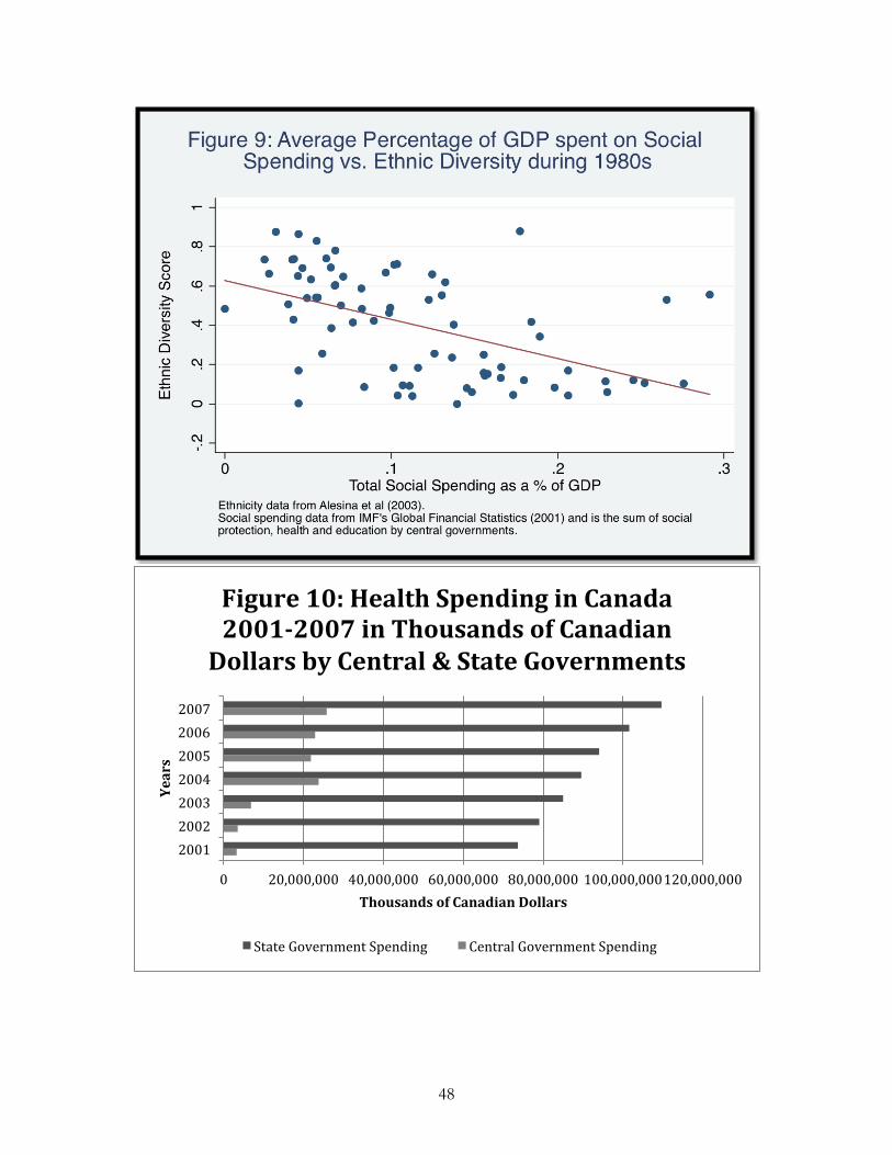
48
0 20,000,000 40,000,000 60,000,000 80,000,000 100,000,000 120,000,000
2001 2002 2003 2004 2005 2006 2007
Thousands of Canadian Dollars
Years
Figure 10: Health Spending in Canada 2001-‐2007 in Thousands of Canadian Dollars by Central & State Governments
State Government Spending Central Government Spending

49
0 50,000,000 100,000,000 150,000,000 200,000,000
2001
2002
2003
2004
2005
2006
2007
Years
Figure 11: Health Spending in Germany 2001-‐2007 in Thousands of Euros
State Goverment Spending National Government Spending
0
5,000,000
10,000,000
15,000,000
20,000,000
25,000,000
30,000,000
35,000,000
1994 1996 1998 2000 2002 2004 2006
Thousands of National Currency
Figure 12: Central Government Healthcare Spending in Israel 1995-‐2005
in Thousands of National Currency
Cash Basis Accrual Basis

50
0 1,000,000 2,000,000 3,000,000 4,000,000 5,000,000 6,000,000 7,000,000 8,000,000 9,000,000
1988 1990 1992 1994 1996 1998 2000 2002 2004 2006
Figure 13: Central Government Healthcare Spending in Finland
1990-‐2005 in Thousands of National Currency
Cash Basis Accrual Basis
0
10,000,000
20,000,000
30,000,000
40,000,000
50,000,000
60,000,000
1988 1990 1992 1994 1996 1998 2000 2002 2004 2006 2008
Thousands of National Currency
Figure 14: Central Government Healthcare Spending in the
Netherlands 1990-‐2007 in Thousands of National Currency
Cash Basis Accrural Basis

51

52

53

CHAPTER 3
EXPLAINING INCOME INEQUALITY: AGRICULTURAL STRUCTURE AND REGIONAL EFFECTS
Introduction
In 2000, of the twenty countries with the most unequal income distributions,
fourteen were from Latin American and the Caribbean. This list includes the region’s most
populous countries: Brazil, Columbia, and Argentina. The average Latin American country
is nearly twice as unequal as the average Eastern European country and 20% more unequal
than the next most unequal region, sub-Saharan Africa. Despite the predictive power of our
core models of income inequality the literature has been unable to account for why there is
such dramatic regional variation. Instead scholars often fall back on regional dummy
variables to improve model fit. In practice this often results in a significant and substantively
large Latin American dummy, an Asian dummy, and/or an African dummy (e.g. (Higgins
and Williamson 1999)(C. Lee 2005)(C. Lee 2005)). While these dummies improve the fit of
the models, the results may hide as much as they show. They beg the question: in what ways
are these regions systematically different that are not captured by our models?
Understanding the answer is essential as income inequality is linked to many important
political, economic and social outcomes including slower economic growth, reduced political
participation, a reduced possibility of democratization, and increased civil and international
conflict.

55
Literature Review: The Causes of Inequality
Kuznets (1955) argued that as societies develop they experience a rise in income
inequality before declining in income inequality. Nielsen (1994) and Nielsen and Alderson
(1995) argue that the Kuznets curve is driven by four factors: the amount of labor in
agriculture, the income differences between the agricultural and industrial sectors, the supply
of educated workers, and the population growth rate. The percentage of labor force in
agriculture is negatively related to income inequality because of the difference in agricultural
and industrial incomes. Agricultural incomes are assumed to be relatively equal because of
the low levels of capital and human capital that are required for traditional agricultural
production. In contrast, incomes in the non-agricultural sector are driven by capital
accumulation and are therefore more variable. The smaller the percentage of labor in
agriculture, the higher income inequality will be as more people are employed in the highly
unequal modern sector. Early studies have found that the percentage of laborers in
agriculture has a significant and robust influence on income inequality (Nielsen
1994)(Nielsen and Alderson 1995). More recently however, Lee (2005) and Lee, Nielsen and
Alderson (2007) have failed to find a significant relationship to income inequality. Changes
in datasets and methods may explain this disparity, but the conflicting conclusions point to a
need for further investigation. The second core explanation of income inequality is the
difference in wages between the agricultural and manufacturing sectors. During the first
stages of development industrial workers have larger incomes than agricultural workers
because of their higher productivity. This income disparity creates a more unequal society.
As workers continue to migrate into the modern sector, society becomes more equal since
more and more workers are employed in the same highly productive modern sector. Third,
population growth increases inequality by creating a large supply of unskilled labor. This

56
large supply of unskilled workers increases the wage difference between unskilled and skilled
work. Similarly, the fourth factor, the supply of educated workers also affects the supply
and demand of labor. Higher school enrollment increases supply of educated workers and
creates competition for high-paying jobs. With more qualified workers available for high-
paying jobs requiring education wages fall for the richest workers thereby reducing income
inequality in society.
Additional variation in cross-national income inequality is usually accounted for by
integration in the global economy, the level of democracy, and ethnic fractionalization. The
literature is divided about the effect of engagement in the global economy on inequality
(Alderson and Nielsen 2002)(Adsera and Boix 2002)(Reuveny and Li 2003)(Mahler
2004)(Brune and Garrett 2005)(Alderson, Beckfield, and Nielsen 2005)(C. Lee, Nielsen, and
Alderson 2007)(Babones and Vonada 2009). When countries engage in globalization, each
country becomes richer on the whole but certain groups benefit and others lose. If the
unequal growth goes towards the poor then globalization will decrease inequality. If it is
shunted towards the rich then this unequal growth will cause an increase in pre-tax
inequality.
Democracy may also impact income inequality (Muller 1988)(Lindert 1994)(Boix
1998)(Boix 2003)(Reuveny and Li 2003)(Rudra 2004)(Rudra and Haggard 2005)(Huber,
Mustillo, and J. D. Stephens 2008). Inequality generates demands by the poor for the
government to redistribute wealth from the rich to them (Meltzer and Richard 1981). In
democratic countries, the government should be more responsive to these pressures to
redistribute than in autocratic countries (Boix 1998)(2003). Democratic countries should
therefore have lower post-tax income inequality. Democracy should also reduce pre-tax
income inequality, as the majority would pass policies that redistributed income to it through

57
preferable policies that shaped the income distribution. The results however have been
mixed. Some studies have shown that democracy reduces inequality (Muller 1988)(Lindert
1994)(Reuveny and Li 2003)(Rudra 2004) many other studies have found democracy to have
no effect on national level income inequality (Bollen and Jackman 1985)(Nielsen
1994)(Nielsen and Alderson 1995)(Deininger and Squire 1996).
Finally, ethnicity may have an impact on income inequality (Moller, Alderson, and
Nielsen 2009). Societies with large ethnic minorities often have a history of oppression and
inequality. This oppression can occur by the minority against the majority or by a majority
against a minority. Either way, increasing ethnic diversity is expected to have a strong
negative effect on income inequality.
Theory
Williamson (1991) notes that despite the overall fit of inverted parabolic relationship
between development and income inequality, there is large unexplained variation. One
problem is the standard model assumes the agricultural sector to be relatively equal
compared to the industrial sector. In some societies this may be true but it need not always
be the case. Agricultural inequality may differ dramatically between different countries and
across regions of the world. The structure of the agricultural sector originates from factor
endowments inherent to specific geographical regions (Sokoloff and Engerman 2000)(2002).
Specific combinations of soil and climate enable different types of crops to grow in different
regions. Some crops are more amendable to plantation style agriculture than others. For
example, large and very profitable sugar plantations in the Caribbean came into being
because conditions there are ideal for sugar cane and because the returns to scale of sugar
production are very high. This created tremendous wealth for the sugar islands, but it also
created highly unequal societies. The contrast is particularly sharp with the northern US and

58
Canada where wheat farming, which had very small returns scale, created fairly equal
societies. Differing factor endowments therefore create very different agricultural
structures.21
Countries with highly unequal agricultural sectors should experience different
trajectories of inequality over the course of economic development than those where
agriculture is comprised of relatively equal agricultural sectors. Land inequality therefore has
a direct effect on incomes within the agricultural sector. In countries with relatively unequal
agricultural sectors, a few large landowners earn most of the income while poor rural
laborers work the farms for low wages. If relatively few people own land, then those owners
will accrue the majority of the agricultural income and income is highly unequally distributed.
On the other hand, if the agricultural structure leads to relatively equal land ownership then
agricultural incomes will also be relatively equal. Income inequality is therefore already very
high in some agricultural countries before development even begins. Instead of becoming
more unequal as they develop, income inequality will moderate as workers migrate from the
agricultural sector to the more equal industrial sector. The high levels of existing agricultural
income inequality therefore alter the inverted u-shape of the relationship between
development and inequality into a linear relationship of decreasing inequality. Conversely,
countries with low agricultural inequality will follow the Kuznets curve.
Understanding how factor endowments shape the agricultural structure present at
the beginning of economic development leads to two hypotheses. First, higher levels of land
inequality will lead to higher levels of income inequality. Second, because land ownership
patterns are clustered by regions of the world, accounting for these similar agricultural
21 Easterly (2007) empirically tests Sokoloff and Engerman’s hypothesis using a large-N analysis. He constructs a “wheat-sugar suitability ration” using United Nations data on temperature and rainfall. This ratio measures the amount of land suitable for wheat production compared to sugar production. Easterly confirms Engerman and Sokoloff’s expectation that countries with land suitable for sugar production are more unequal.

59
structures will reduce or eliminate significant and substantial regional dummies that
numerous studies of income inequality have found (e.g. (Higgins and Williamson 1999)(C.
Lee 2005)(C. Lee 2005)).
Data
The dependent variable is pre-tax income inequality. Income inequality is the
distribution of incomes within a particular country and is operationalized using a gini
coefficient. Gini coefficients measure inequality by locating a distribution between two
idealized states of the world: perfect equality, where everyone in the group has the same
amount of a good (measured as zero), and perfect inequality, where one individual has all of
the good and no one else has any (measured as one).22 The more income earned by fewer
people, the higher the gini score will be. For example, in 2000 the world’s most unequal
country (pre-tax) was South Africa (gini = .75) and the most equal was Slovenia (gini =
.32)(Solt 2009).
I use Solt’s (2009) recently released income inequality dataset, Standardizing the
World Income Inequality Database (SWIID).23 SWIID is an update of the commonly used
World Income Inequality Database (WIID) a collection of hundreds of national level
inequality studies (UNU-WIDER 2008). The WIID has been widely criticized for its use of
apples and oranges measures and spotty coverage (Brune and Garrett 2005). Solt addresses
these concerns by making a series of standardizing assumptions. Using these assumptions
22 Formally a gini coefficient is the area above the Lorenz curve and below a 45-degree line from the origin to the point (1,1) divided by the total area below the 45-degree line. The Lorenz curve is constructed on a graph where the x-axis is represents the sample population lined up with the poorest person on the left (x = 0) and the richest person or group on the right (x = 1). The y-value for each point on the x-axis is the percentage of the total possessed by that person or group and all of those poor than that point. This series of points forms a curve that begins at the origin (0,0), ends at (1,1) and is always equal to or below the 45-degree line. 23 Other widely cited databases are also available for reference (Deininger and Squire 1996)(Deininger and Squire 1998). These sources draw on the same primary data, the WIID.

60
he has standardized the scores and has drawn inferences from the primary data to fill
missing measurements when appropriate.
The independent variable of interest is land inequality. Similar to income inequality,
agricultural inequality is the distribution of agricultural production in a given society. Like
income inequality, it can also be measured using a gini coefficient ranging between zero and
one. One means of capturing agricultural inequality is to look at how farm size is distributed
amongst farmers in a country. The distribution of farm size can be converted into a measure
of land inequality using a gini coefficient. Land inequality scores range from Venezuela
(.857), which has the highest score, to Singapore (.291), which has the lowest score. Land
inequality data is drawn from the Food and Agriculture Organization’s (FAO) World Census of
Agriculture. Frankema (2009) combines FAO data with data from the International Institute
of Agriculture to produce the most complete, publicly available, land inequality dataset
covering 105 countries.24 Landholding data measures the amount of land per farm and
therefore the ability of the farmer to produce agricultural income. While the depth of
coverage varies, Frankema made specific efforts to capture a post-independence measure for
former colonies, a contemporary measure, and historical measures if possible. Generally,
land inequality does not vary widely within a country except in times of land reform like the
Taiwanese and Korean land reforms in the 1950s (Frankema and Smits 2005)(Jeon and Kim
2000). Because land inequality data measures farming inequality and not land ownership
24 Other major indices of land inequality include Taylor and Hudson’s dataset of 54 countries with data-points circa 1960 (Taylor and Hudson 1972). Deininger and Squire (1998) have a land inequality dataset with 261 observations of 103 countries, however only 60 observations have been published (Deininger and Olinto 2000).

61
inequality,25 his measures of land inequality are lower-bound measures of actual agriculture
income inequality.
Four core variables have been shown to have significant effects on income inequality
(Nielsen 1994)(Nielsen and Alderson 1995). Labor force in agriculture is drawn from the World
Development Indicators (WDI) published by the World Bank (2008). Based on conflicting
results from previous research it is expected to have an indeterminate effect. The measure
of sector dualism captures the inequality of productivity between the agricultural sector and the
modern sector. Nielsen defines sector dualism to be |p – L| where p is the percentage of the
labor force employed in agriculture and L is the agriculture share of GDP. If the percentage
of GDP produced by agriculture and the percentage of the population employed by
agriculture are equal, then sector dualism, by definition, takes a value of zero. An increase in
sector dualism is expected to increase inequality. Both figures are drawn from the WDI. The
supply of educated labor, I use the percentage of the population that has attended some level
of high school. This data is drawn from Barro and Lee (1996)(2001). Barro and Lee provide
the data at five-year increments. I generate values for the intervening years using a linear
function. An increase in population growth is expected to increase inequality and the data is
drawn from the WDI.
Ethnicity is drawn from Alesina et al’s (2003) measure of ethnic fractionalization. It
ranges from zero to one with higher scores indicating a higher level of ethnic diversity in a
society. In order to control for the effect of integration into the world economy, or
globalization, which is expected to increase inequality, I generate two variables. The first
variable, trade, is imports plus exports and divided by GDP. The second variable, foreign direct
25 Landownership may be a more appropriate measure but is unavailable. Farming inequality measures the distribution of farmland by units farmed by particular farmers. Landowners may rent their properties to multiple farmers and accrue profits from each of them.

62
investment (FDI), is the sum of inflows plus outflows. Data for both variables are drawn from
the WDI.
In order to control for the equalizing effect of democracy, I follow Huber, Stephens
and Mustillo’s (2008) example and create a variable measuring the cumulative years of
democracy since 1945. I use Marshall and Jagger’s Polity IV data to construct the variable
(Marshall and Jaggers 2008).26 Each year for which a country scores seven or greater is
counted as a year of democracy. The variable is the total years of democracy since 1945.
Methods
The resulting panel data runs from 1980 to 2007 and includes 892 observations over
74 different countries. The largest sample in any one cross-section is considerably smaller
than 74 countries (~45). To analyze the data, I use a random effects model with unbalanced
panel data. While random effects risks overestimating the significance of the results, it is an
appropriate choice because one of the independent variables, ethnicity, is time-invariant. The
other option, a fixed effects model, would cause ethnicity to drop out of the model.
Analysis & Results
Does agricultural structure fundamentally alter our understanding of how income
inequality changes over the course of development? Figure 17 shows this relationship
between income inequality and development using data from 1960 to 2005. For both
graphs, the x-axis is the natural logarithm of GDP per capita and the y-axis is income
inequality. The left-hand graph displays the relationship for country-year observations where
land inequality is amongst the highest 25% of scores in the sample. For these high land
inequality countries there is a negative linear relationship. The right hand graph displays the
26 Each country scored on a scale of -10 to 10 where -10 is the most authoritarian and 10 is the most democratic.

63
remainder of the observations and shows that the classic Kuznets relationship holds for
countries where land inequality is not extremely high.
To see if this patter withstands the inclusion of other control variables Table 6 shows
the results for four models that test land inequality alongside standard explanations of
income inequality. Model 1 includes the four core variables from previous research. Model
2 then includes land inequality as a predictor. Land inequality is statistically significant at the
.001 level. Substantively, an increase in from one-standard-deviation below the mean to
one-standard-deviation above the mean in land inequality would cause the income inequality
of a country to increase of .09. Since the average income inequality gini is .48 in 1990 then
increasing from .39 to .56 is an 18% increase in income inequality.
The results for the core variables in Models 1 & 2 are somewhat consistent with
previous findings. The positive association between increased sector dualism and increasing
income inequality match the expectations and findings from the literature. An increase of the
population in agriculture is strongly associated with a decrease in inequality in both models. The
other variables run counter to expectations. An increase in secondary school enrollment
corresponds with an increase in inequality in both models. Population growth is not statistically
significant in either model.
Model 3 includes other explanations of income inequality (ethnicity, trade, foreign direct
investment, and democracy) but excludes land inequality. Model 4 then adds land inequality to
Model 3. Land inequality continues to be a significant predictor of income inequality in the
presence of these four new variables.
The new variables have a mixed performance. Ethnicity has the predicted sign, is
statistically significant and has a large substantive impact. An increase in ethnic diversity is
associated with an increase in inequality in both models. FDI is indeterminate in both

64
Models 3 and 4. Trade is negatively correlated with income inequality. This is not a result of
either increased industrial employment or wages as both mechanisms are accounted for in
other control variables. Instead governments may be compensating groups to maintain
support for free trade. Democracy is associated with a marked increase in inequality in both
models. This is an unexpected outcome but the relationship between democracy and
income inequality is clear from the data. The relationship is robust different constructions
of the democracy variable.27 In fact, models that only include democracy and income
inequality produce strong and positive correlations with income inequality. Secondary
enrollment becomes significant and is positively related to income inequality when land inequality is
included. Population in agriculture continues to decrease inequality in Model 3 but is statistically
insignificant in the presence of land inequality. Population growth significantly increases
income inequality in both models.
The second hypothesis is that agricultural structure will explain why income
inequality is so similar within regions. Income inequality varies significantly between regions
as shown in Figure 18, which displays the box plots of income inequality by region for 106
countries in 2000. Each solid blue box represents half the sample. The bottom edge is the
25th percentile and the top edge is the 75th percentile. The blue line in the center represents
the median value for the region. The “whiskers” above and below each box represent the
highest and lowest values that are 1.5 times the interquartile range respectively. The dots
above and below some of the boxes represent outliers that fall outside of this range (Cox
2009). As one might expect, different regions display different levels and distributions.
27 The variable in the analysis is cumulative years of democracy. Because the effect of democracy might decrease marginally over time I also ran the analysis with logarithm of cumulative years of democracy. This means that the initial years of democracy were counted more than years in the future. The results are not altered substantially by using the natural logarithm of the cumulative years score, a log-base-10 version, nor the raw Polity scores.

65
Both Sub-Saharan Africa and Latin America and the Caribbean standout as have
substantially higher income inequality than the remaining regions.
As with income inequality, there are significant differences in land inequality between
different regions of the world. Figure 19 displays the box plot of land inequality by region.
Latin America is far and away the most unequal region in terms of land distribution. The
OECD is the next most unequal but has significantly more dispersion. Sub-Saharan Africa
has the largest range of land inequality. It has the second most unequal country outside of
Latin America (Swaziland, .835) but also has the second most equal country in the sample
(Niger, .312).
The distinct regional patterns displayed in Figures 18 and 19 suggest that land
inequality may be the key to understanding why many studies of income inequality are
unable to explain away significant regional dummies. Latin America and the Caribbean have
had the highest levels of income inequality and the highest levels of land inequality. Of the
85 countries with land and income inequality scores in 2000, 16 of the 20 most land unequal
countries are from Latin America and the Caribbean and 14 of the 20 countries with the
highest income inequality are from Latin America and the Caribbean as shown in Table 7.
The next table, Table 8, shows how regional dummies impact the core model and
how land inequality affects the predictive power of these regional dummies. The overall
message is that regional dummies for Latin America and Sub-Saharan Africa have a large and
statistically significant impact on income inequality while the East Asia and Pacific dummy
does not. Models 5 and 6 examine the impact of land inequality on the Latin American
dummy. Model 5 shows that the Latin American dummy has a large and significant effect
on income inequality. Recall from Figure 18 that Latin America is the world’s most unequal
region. Model 6 shows that land inequality is neither able to account for this dummy

66
variable nor is it significant in its own right with paired with a Latin America and Caribbean
dummy. Statistically, it is problematic that Latin America has both the highest levels of land
inequality and the highest levels of income inequality because they are highly collinear. In
Model 6 land inequality is statistically insignificant. Figure 20 helps us understand why. In
Figure 20 the “x” points represent the Latin American and Caribbean countries (LACs).
The dots display the remaining observations from around the world. The x-axis is land
inequality and the y-axis is income inequality. When LACs are included then there is a
positive relationship between land inequality and income inequality as shown by the solid
regression line. When LACs are excluded the regression line flattens substantially as shown
by the dotted regression line. Removing LACs therefore removes the predictive power of
land inequality from the model. Within the LAC observations there is not clear relationship
between land inequality and income inequality. Because there is not a clear relationship
between the two, it makes sense that including land inequality does not restrict the predictive
power of the Latin American dummy.
Models 7 and 8 look at the impact of land inequality on a Sub-Saharan Africa
dummy. Land inequality is significant in its own right in Model 8. It also reduces the
predictive power of the Sub-Saharan Africa regional dummy by about ten percent. It does
not prevent it from being statistically significant. Land inequality is less useful explaining
why sub-Saharan Africa is highly unequal than it is in explaining Latin American
exceptionalism. Primary research on the specific roots of land inequality is largely limited to
the Americas but has been extended to other regions. Particularly, van de Walle (2009)
addresses the roots of African inequality. In settler dominated societies (Kenya, South
Africa, Rhodesia) he concurs with analysis of Engerman and Sokoloff, that large scale
agricultural production created the foundation for institutions that continued to create

67
inequality. However, in analyzing the remainder of sub-Saharan Africa, van de Walle argues
that poor institutions are a function of original endowments only in the sense that Africa was
neither labor nor resource rich. Little European penetration of African societies, a poor
transition to self-government, and huge intra-country regional differences all contributed to
African inequality by creating incentives for the predatory state so common in sub-Saharan
Africa. He concludes, "Inequality should be understood as a side product of a process of
elite formation in the states of the region" (309). Because land inequality is only driving
inequality for a few countries in Africa, land inequality does not remove much of the
explanatory power of the African dummy.
Table 5 provides descriptive statistics of land inequality measures in sub-regions of
Africa. Interestingly, West and Central Africa have relatively low land inequality scores
compared to South and East Africa. This is consistent with van de Walle’s (2009)
expectation that low European penetration into these areas would create entirely different
dynamics than those in the settler states of South and East Africa that were more amenable
to plantation style agriculture.
Models 9 and 10 look at the impact of an East Asia and Pacific dummy. The dummy
is not significant in either model. Land inequality is statistically significant in its own right.
Within Models 5-10 the other control variables perform consistently on the whole. Ethnicity
remains a powerful predictor of increased inequality. Sector dualism, population growth, and
democracy remain positive predictors of inequality. Population in agriculture is negatively related
to inequality. Secondary enrollment is an inconsistent predictor of income inequality but is
occasionally significantly related to a decrease in income inequality.

68
Conclusion
The structure of agriculture is important for understanding how income inequality
changes over the course of development. For countries with high levels of land inequality
the process of industrialization creates a consistent movement towards equality. This is a
sharp contrast to the traditional Kuznet’s curve experienced by countries with more equal
agricultural sectors. Land inequality is also helpful for understanding the regional nature of
inequality. Latin America is the most unequal region in terms of both land inequality and
income inequality.
One limiting factor of this study is the range of available data. Many of the control
variables presented in the analysis have effects that are contradictory to expectations from
previous research. This could be a function of the range of available data. For example,
multiple authors have theorized that democratization will cause greater redistribution. The
results found here indicate that democracy actually creates more inequality in society.
During the last 15 years the worlds most developed nations have seen an increase in
inequality (Alderson and Nielsen 2002)(Kenworthy and Pontusson 2005)(Brandolini and
Smeeding 2006). It would be helpful to be able to include pre-1980s data in the sample to
see if democracy has consistently increased inequality or if this effect is only present in the
period covered by the sample.
Another puzzle raised by this research is why land inequality is such a powerful
predictor of income inequality between regions but not within some of them. For example,
within Sub-Saharan African countries land inequality is a statistically significant predictor of
income inequality. In contrast, while land inequality is very high within Latin America and
the Caribbean as a whole, land inequality does a poor job of explaining income inequality
within Latin America and the Caribbean. This points out an interesting irony in regionally

69
focused research. Scholars of Latin American inequality would conclude that land inequality
has no effect on income inequality despite it being the best predictor of Latin American
exceptionalism. In contrast scholars studying other regions of the world will see their
models improve as they include land inequality in their regional analyses.
Finally, several of the variables present in this analysis are affected by land inequality.
Land inequality affects education levels and is likely to affect democratization. The
democratization literature discusses the role of immobile factors in the democratization
process. Agriculture is truly an immobile factor in a world with high agricultural tariffs.
Land inequality provides a handle of the political power of a particularly immobile sector.
When agriculture is concentrated in the hands of the few, then landowners should be more
powerful as a group. Land inequality may help us understand when democratization is and
is not successful. This study has bracketed these relationships between land inequality and
other independent variables in the model, but a subsequent study might more fully explore
and specify the relationships between the various independent variables.

70

71

72

73
Table 5: Descriptive Statistics of Land Ginis by Region
Table From Frankema (2009) Min Max Median Mean St. Dev Obs South America 63.9 86.3 80.4 70.9 6.3 11 Central America 60.7 78.3 73.9 72.3 6.0 7 Caribbean 46.2 81.6 69.9 68.1 11.8 7 East Asia 30.7 43.8 39.5 38.4 5.5 4 South Asia 41.8 62.3 55.4 53.7 8.7 6 South East Asia 29.1 68.0 47.3 47.9 11.7 8 North Africa & Middle East 56.3 82.0 63.8 65.1 7.3 12 South and East Africa 36.8 83.5 66.7 62.7 17.4 12 West and Central Africa 31.2 68.1 45.2 45.2 9.1 14 Western Offshoots 47.0 78.6 61.1 61.9 16.4 4 Western Europe 47.0 79.1 63.4 63.9 10.1 14 Eastern Europe 39.2 60.0 52.4 51.0 9.5 4 Scandinavia 42.1 63.3 47.2 49.3 7.5 8
World 29.1 86.3 60.0 59.7 15.0 111

74

75
Table 7: Twenty Most Unequal Countries in 2000
Listed by Level of Inequality. (Bolded entries appear in both lists).
Highest Income Inequality Highest Land Inequality
South Africa Venezuela Burkina Faso Paraguay Zambia Chile Swaziland Swaziland Brazil Panama Bolivia Argentina Paraguay Peru Chile Australia Haiti Madagascar Ecuador Spain Guatemala Brazil Honduras Uruguay Panama Tanzania Colombia El Salvador Uganda Ecuador El Salvador Guatemala Cameroon Bolivia Argentina Nicaragua Puerto Rico Jamaica Nicaragua Dominican Republic Countries for which both income inequality and land inequality measures exist in 2000. Income inequality from Solt (2009). Land inequality from Frankema (2009).

76

77
Appendix I
The Influence of Diversity on Specific Kinds of Social Spending
The effects of ethnicity on social protection spending are much more pronounced
than they are on overall spending, as shown in Table 4 below. Social protection is much
more likely to occur at the central government level compared to education or healthcare
spending which often occur at the regional or local levels of government. Social protection
figures therefore most closely match the level of the data (central government expenditures)
to the level of the key independent variable (national level ethnic diversity figures). Model 6
shows that ethnicity has a statistically significant negative effect on social protection
spending by general government in the 2000s. This Table 3 displays the results. Ethnic
Diversity has a consistent negative impact on social protection in every decade except the
1970s.
In contrast to spending on social protection, spending on health and education is
much more likely to occur at the sub-national level. Since ethnicity is only captured at the
national level one would expect the mismatch of the data to reduce the predictive power of
the models. Table 4 tests to see whether or not ethnicity has a negative impact on healthcare
expenditures. The results in Table 4 are less predictive than their counterparts in Table 3.
The key variable of interest, ethnicity, is only significant in the 1990s significant in each of the
models. Table 5 tells a similar story for education. Ethnicity is less statistically significant and
less substantively important in predicting spending on education than it was on social
protection.
Taken as a whole, Tables 3, 4, and 5 support the idea that there is a substantial and
statistically significant and negative effect of ethnicity on social spending. This effect is
strongest on social protection expenditures but still exists for education and health

78
expenditures.

79

80

81

82
The following three tables test the hypothesis that ethnic diversity has a curvilinear
effect on social spending for each sub-type of social spending (healthcare, education and
social protection).

83

84

85
Appendix II:
Change in Countries Reporting Central Government Spending Data over Time

86
BIBLIOGRAPHY Acemoglu, Daron, and James A. Robinson. 2006a. “De Facto Political Power and
Institutional Persistence.” American Economic Review 96(2): 325-220. ———. 2006b. “Economic Backwardness in Political Perspective.” American Political Science
Review 100(01): 115-131. ———. 2000. “Why Did the West Extend the Franchise? Democracy, Inequality, and
Growth in Historical Perspective.” The Quarterly Journal of Economics 115(4): 1167-1199.
Adsera, Alicia, and Carles Boix. 2002. “Trade, Democracy, and the Size of the Public Sector:
The Political Underpinnings of Openness.” International Organization 56(2): 229-262. Alderson, Arthur S., Jason Beckfield, and François Nielsen. 2005. “Exactly How Has
Income Inequality Changed?: Patterns of Distributional Change in Core Societies.” International Journal of Comparative Sociology 46(5-6): 405-423.
Alderson, Arthur S., and François Nielsen. 2002. “Globalization and the Great U-Turn:
Income Inequality Trends in 16 OECD Countries.” American Journal of Sociology 107(5): 1244-1299.
Alesina, Alberto, Reza Baqir, and William Easterly. 1999. “Public Goods and Ethnic
Divisions.” The Quarterly Journal of Economics 114(4): 1243-1284. Alesina, Alberto et al. 2003. “Fractionalization.” Journal of Economic Growth 8(2): 155-194. Alesina, Alberto, and Edward L Glaeser. 2004. Fighting Poverty in the US and Europe: A World of
Difference. Oxford: Oxford University Press. Alesina, Alberto, Edward L. Glaeser, and Bruce Sacerdote. 2001. “Why Doesn't The US
Have a European-Style Welfare State?.” National Bureau of Economic Research (NBER). Avelino, George, David S. Brown, and Wendy Hunter. 2005. “The Effects of Capital
Mobility, Trade Openness, and Democracy on Social Spending in Latin America, 1980-1999.” American Journal of Political Science 49(3): 625-641.
Babones, Salvatore J., and Dorian C. Vonada. 2009. “Trade globalization and national
income inequality -- are they related?.” Journal of Sociology 45(1): 5-30. Banerjee, Abhijit, and Lakshmi Iyer. 2005. “History, Institutions, and Economic
Performance: The Legacy of Colonial Land Tenure Systems in India.” American Economic Review 95(4): 1190-1213.
Barro, Robert J., and Jong-Wha Lee. 2001. “International data on educational attainment:
updates and implications.” Oxf. Econ. Pap. 53(3): 541-563.

87
———. 1996. “International Measures of Schooling Years and Schooling Quality.” The
American Economic Review 86(2): 218-223. Bates, Robert H. 1981. Markets and States in Tropical Africa: The Political Basis of Agricultural
Policies. Berkeley: University of California Press. Beck, Thorsten et al. 2001. “New tools in comparative political economy: The Database of
Political Institutions.” World Bank Economic Review 15(1): 165-176. Blackmon, Douglas A. 2008. Slavery by Another Name: The Re-Enslavement of Black People in
America from the Civil War to World War II. New York: Doubleday. Boix, Carles. 2003. Democracy and Redistribution. Cambridge: Cambridge University Press. ———. 1998. Political Parties, Growth and Equality: Conservative Andsocial Democratic Economic
Strategies in the World Economy. Cambridge: Cambridge University Press. Bollen, Kenneth A., and Robert W. Jackman. 1985. “Political Democracy and the Size
Distribution of Income.” American Sociological Review 50(4): 438-457. Brambor, Thomas, William Roberts Clark, and Matt Golder. 2006. “Understanding
Interaction Models: Improving Empirical Analyses.” Political Analysis 14(1): 63-82. Brandolini, Andrea, and Timothy M. Smeeding. 2006. “Patterns of Economic Inequality in
Western Democracies: Some Facts on Levels and Trends.” PS: Political Science & Politics 39(01): 21-26.
Brooks, Sarah Marie. 2009. Social Protection and the Market in Latin America: The Transformation of
Social Security Institutions. Cambridge: Cambridge University Press. Brune, Nancy, and Geoffrey Garrett. 2005. “The Globalization Rorschach Test:
International Economic Integration, Inequality, and the Role of Government.” Annual Reviews in Political Science 8: 399-423.
Cederman, Lars-Erik, Brian Min, and Andreas Wimmer. 2009. “Ethnic Power Relations
dataset.” http://hdl.handle.net/1902.1/11796. Cohen, William. 1991. At Freedom's Edge: Black Mobility and the Southern White Quest for Racial
Control, 1861-1915. Baton Rouge: Louisiana State University Press. Collier, Paul, Patrick Honohan, and Karle Ove Moene. 2001. “Implications of Ethnic
Diversity.” Economic Policy 16(32): 129-166. Cox, N. J. 2009. “Speaking Stata: Creating and varying box plots.” Stata Journal 9(3): 478-496. Deininger, Klaus, and Lyn Squire. 1996. “A New Data Set Measuring Income Inequality.”
World Bank Econ Rev 10(3): 565-591.
88
———. 1998. “New ways of looking at old issues: inequality and growth.” Journal of
Development Economics 57(2): 259-287. Deininger, Klaus W, and P. Olinto. 2000. “Asset Distribution, Inequality, and Growth.”
World Bank Policy Research Working Paper 2375. Easterly, William. 2007. “Inequality does cause underdevelopment: Insights from a new
instrument.” Journal of Development Economics 84(2): 755-776. Easterly, William, and Ross Levine. 1997. “Africa's Growth Tragedy: Policies and Ethnic
Divisions.” The Quarterly Journal of Economics 112(4): 1203-1250. Engerman, Stanley L., Elisa Mariscal, and Kenneth L. Sokoloff. 2009. “The evolution of
schooling in the Americas, 1800-1925.” In Human Capital and Institutions: A Long-Run View, eds. David Eltis, Frank D. Lewis, and Kenneth L. Sokoloff. Cambridge University Press.
Engerman, Stanley L., and Kenneth L. Sokoloff. 2002. “Factor Endowments, Inequality, and
Paths of Development among New World Economies.” Economía 3(1): 41-109. Fearon, James D. 2003. “Ethnic and Cultural Diversity by Country.” Journal of Economic
Growth 8(2): 195-222. Fearon, James D., Kimuli Kasara, and David D. Laitin. 2007. “Ethnic Minority Rule and
Civil War Onset.” American Political Science Review 101(01): 187-193. Frankema, Ewout. 2009. “The Colonial Origins of Inequality: Exploring the Causes and
Consequences of Land Distribution.” In Poverty, Inequality, and Policy in Latin America, CESifo seminar series, eds. Stephan Klasen and Felicitas Nowak-Lehmann D. Cambridge, Mass: MIT Press.
Frankema, Ewout, and Jan-Pieter Smits. 2005. “Exploring the Historical Roots of Eastern
Asia's Post-War Catch-Up Growth: A Trade Perspective, 1906-1999.” Journal of the Asia Pacific Economy 10(2): 178-194.
Galor, Oded, Omer Moav, and Dietrich Vollrath. 2009. “Inequality in Landownership, the
Emergence of Human-Capital Promoting Institutions, and the Great Divergence.” Review of Economic Studies 76(1): 143-179.
Gerschenkron, Alexander. 1943. Bread and Democracy in Germany. Ithaca: Cornell University
Press. Goodhart, David. 2004. “Too Diverse?.” Prospect Magazine (95). Greenwood, Michael J. 1971. “An analysis of the determinants of internal labor mobility in
India.” The Annals of Regional Science 5(1): 137-151.

89
———. 1975. “Research on Internal Migration in the United States: A Survey.” Journal of Economic Literature 13(2): 397-433.
Habyarimana, James et al. 2007. “Why Does Ethnic Diversity Undermine Public Goods
Provision?.” American Political Science Review 101(04): 709-725. Haggard, Stephan, and Robert R Kaufman. 2008. Development, Democracy, and Welfare States:
Latin America, East Asia, and Eastern Europe. Princeton: Princeton University Press. Higgins, Matthew, and Jeffrey G. Williamson. 1999. “Explaining Inequality the World
Round: Cohort Size, Kuznets Curves, and Openness.” SSRN eLibrary. http://papers.ssrn.com/sol3/papers.cfm?abstract_id=173408 (Accessed May 16, 2009).
Hiscox, Michael J. 2001. “Class Versus Industry Cleavages: Inter-Industry Factor Mobility
and the Politics of Trade.” International Organization 55(01): 1-46. ———. 2002. International Trade and Political Conflict: Commerce, Coalitions, and Mobility.
Princeton, N.J: Princeton University Press. Horowitz, Donald L. 2000. Ethnic Groups in Conflict. 2nd ed. Berkeley, Calif: University of
California Press. Huber, Evelyne, Thomas Mustillo, and John D. Stephens. 2008. “Politics and Social
Spending in Latin America.” Journal of Politics 70(2): 420-436. Huber, Evelyne, and Frank Safford, eds. 1995. Agrarian Structure & Political Power: Landlord &
Peasantin the Making of Latin America. Pittsburgh: University of Pittsburgh Press. Huber, Evelyne, and John D. Stephens. 2001. Development and Crisis of the Welfare State: Parties
and Policies in Global Markets. Chicago: University of Chicago Press. Huntington, Samuel P. 2004. “The Hispanic Challenge.” Foreign Policy (141): 30-45. Inglot, Tomasz. 2008. Welfare States in East Central Europe, 1919-2004. Cambridge: Cambridge
University Press. International Monetary Fund. 2010a. International Financial Statistics.
http://www.imfstatistics.org.libproxy.lib.unc.edu/imf/. ———. 2010b. World Economic Outlook Database.
http://www.imf.org/external/ns/cs.aspx?id=28. International Monetary Fund. Statistics Department. 2010. Government finance statistics.
Washington, DC: International Monetary Fund. Jensen, Carsten, and Svend-Erik Skaaning. 2010. “Democracy, Ethnic Fractionalization, and
the Politics of Social Spending.” Unpublished.

90
Jeon, Yoong-Deok, and Young-Yong Kim. 2000. “Land Reform, Income Redistribution,
and Agricultural Production in Korea.” Economic Development and Cultural Change 48(2): 253-268.
Kaufman, Robert R., and Alex Segura-Ubiergo. 2001. “Globalization, Domestic Politics, and
Social Spending in Latin America: A Time-Series Cross-Section Analysis, 1973-97.” World Politics 53(4): 553-587.
Kenworthy, Lane, and Jonas Pontusson. 2005. “Rising Inequality and the Politics of
Redistribution in Affluent Countries.” Perspectives on Politics 3(03): 449-471. Khan, Abdul, and Stephen Mayes. 2009. Transition to Accrual Accounting. Fiscal Affairs
Department, IMF. Klor, Esteban F., and Moses Shayo. 2010. “Social identity and preferences over
redistribution.” Journal of Public Economics 94(3-4): 269-278. Kuznets, Simon. 1955. “Economic Growth and Income Inequality.” The American Economic
Review 45(1): 1-28. Ladewig, Jeffrey W. 2006. “Domestic Influences on International Trade Policy: Factor
Mobility in the United States, 1963 to 1992.” International Organization 60(01): 69-103. Laitin, David D., and Daniel N Posner. 2001. “The Implications of Constructivism for
Constructing Ethnic Fractionalization Indices.” APSA-CP: Newsletter of the Organized Section in Comparative Politics of the American Political Science Association 12(Winter): 13-17.
Lee, Cheol-Sung. 2005. “Income Inequality, Democracy, and Public Sector Size.” American
Sociological Review 70(1): 158-181. Lee, Cheol-Sung, François Nielsen, and Arthur S. Alderson. 2007. “Income Inequality,
Global Economy and the State.” Social Forces 86(1): 77-111. Lind, Jo Thori. 2007. “Fractionalization and the Size of Government.” Journal of Public
Economics 91(1-2): 51-76. Lindert, Peter H. 2004. Growing Public: Social Spending and Economic Growth Since the Eighteenth
Century. Cambridge, UK: Cambridge University Press. Lindert, Peter H. 1994. “The Rise of Social Spending, 1880-1930.” Explorations in Economic
History 31(1): 1-37. Luttmer, Erzo F. P. 2001. “Group Loyalty and the Taste for Redistribution.” Journal of
Political Economy 109(3): 500-528. Mahler, Vincent A. 2004. “Economic Globalization, Domestic Politics, and Income

91
Inequality in the Developed Countries: A Cross-National Study.” Comparative Political Studies 37(9): 1025-1053.
Mariscal, Elisa, and Kenneth L. Sokoloff. 2000. “Schooling, suffrage, and the persistence of
inequality in the Americas, 1800–1945.” In Political Institutions and Economic Growth in Latin America: Essays in Policy, History, and Political Economy, ed. Stephen H Haber. Stanford, Calif: Hoover Institution Press, Stanford University, p. 294.
Marshall, Monty G., and Keith Jaggers. 2008. Polity IV Dataset. College Park: University of
Maryland, Center for International Development and Conflict Management. http://www.systemicpeace.org/polity/polity4.htm (Accessed March 21, 2009).
Meltzer, Allan H., and Scott F. Richard. 1981. “A Rational Theory of the Size of
Government.” The Journal of Political Economy 89(5): 914-927. Moller, Stephanie, Arthur S. Alderson, and François Nielsen. 2009. “Changing Patterns of
Income Inequality in U.S. Counties, 1970–2000.” American Journal of Sociology 114(4): 1037-1101.
Moore, Barrington. 1966. Social Origins of Dictatorship and Democracy: Lord and Peasant in the
Making of the Modern World. Boston: Beacon Press. Mukherjee, Bumba, Dale L. Smith, and Quan Li. 2009. “Labor (Im)mobility and the Politics
of Trade Protection in Majoritarian Democracies.” The Journal of Politics 71(01): 291-308.
Muller, Edward N. 1988. “Democracy, Economic Development, and Income Inequality.”
American Sociological Review 53(1): 50-68. Nielsen, François. 1994. “Income Inequality and Industrial Development: Dualism
Revisited.” American Sociological Review 59(5): 654-677. Nielsen, François, and Arthur S. Alderson. 1995. “Income Inequality, Development, and
Dualism: Results from an Unbalanced Cross-National Panel.” American Sociological Review 60(5): 674-701.
Olson, Mancur. 1965. The Logic of Collective Action; Public Goods and the Theory of Groups.
Cambridge, Mass: Harvard University Press. Posner, Daniel N. 2004. “Measuring Ethnic Fractionalization in Africa.” American Journal of
Political Science 48(4): 849-863. Poterba, James M. 1997. “Demographic structure and the political economy of public
education.” Journal of Policy Analysis and Management 16(1): 48-66. Reuveny, Rafael, and Quan Li. 2003. “Economic Openness, Democracy, and Income
Inequality: An Empirical Analysis.” Comparative Political Studies 36(5): 575-601.

92
Rudra, Nita. 2008. Globalization and the race to the bottom in developing countries: who really gets hurt? Cambridge, UK: Cambridge University Press.
———. 2004. “Openness, Welfare Spending, and Inequality in the Developing World.”
International Studies Quarterly 48(3): 683-709. ———. 2007. “Welfare States in Developing Countries: Unique or Universal?.” Journal of
Politics 69(2): 378-396. Rudra, Nita, and Stephan Haggard. 2005. “Globalization, Democracy, and Effective Welfare
Spending in the Developing World.” Comparative Political Studies 38(9): 1015-1049. Rueda, David. 2005. “Insider–Outsider Politics in Industrialized Democracies: The
Challenge to Social Democratic Parties.” American Political Science Review 99(01): 61-74. ———. 2007. Social Democracy Inside Out: Partisanship and Labor Market Policy in Industrialized
Democracies. Oxford: Oxford University Press. Rueschemeyer, Dietrich, Evelyne Stephens, and John D. Stephens. 1992. Capitalist
Development and Democracy. Chicago: University of Chicago Press. Sjaastad, Larry A. 1962. “The Costs and Returns of Human Migration.” The Journal of Political
Economy 70(5): 80-93. Sokoloff, Kenneth L., and Stanley L. Engerman. 2000. “History Lessons: Institutions,
Factors Endowments, and Paths of Development in the New World.” The Journal of Economic Perspectives 14(3): 217-232.
Solt, Frederick. 2009. “Standardizing the World Income Inequality Database.” Social Science
Quarterly 90(2): 231-242. Stephens, John D. 1979. “Class Formation and Class Consciousness: A Theoretical and
Empirical Analysis with Reference to Britain and Sweden.” The British Journal of Sociology 30(4): 389-414.
Taylor, Charles Lewis, and Michael C Hudson. 1972. World Handbook of Political and Social
Indicators. 2nd ed. New Haven: Yale University Press. UNU-WIDER. 2008. “World Income Inequality Database, Version 2.0c.”
http://www.wider.unu.edu/research/Database/en_GB/database/ (Accessed May 22, 2009).
USSR. 1964. Atlas Narodova Mira. Moscow: Department of Geodesy and Cartography of the
State Geological Committee of the USSR. van de Walle, Nicolas. 2009. “The Institutional Origins of Inequality in Sub-Saharan Africa.”
Annual Review of Political Science 12: 307-327.

93
Wegenast, Tim. 2010. “Cana, Café, Cacao: Agrarian Structure and Education in Brazil.” Journal of Iberian and Latin American Economic History 28(1): 103-137.
———. 2009. “The Legacy of Landlords: Educational Distribution and Development in a
Comparative Perspective.” Comparative Governance and Politics 3(1): 81-107. Wilensky, Harold L. 1975. The Welfare State and Equality: Structural and Ideological Roots of Public
Expenditures. Berkeley: University of California Press. Williamson, Jeffrey G. 1991. Inequality, Poverty, and History: The Kuznets Memorial Lectures.
Cambridge, Mass., USA: Blackwell. World Bank. 2008. World Development Indicators (WDI). Zhao, Yaohui. 1997. “Labor Migration and Returns to Rural Education in China.” American
Journal of Agricultural Economics 79(4): 1278-1287.