The Burden of Knowledge and the �Death of the RenaissanceMan�: Is Innovation Getting Harder?�

Benjamin F. Jonesy

April 2008

Abstract

This paper investigates a possibly fundamental aspect of technological progress. Ifknowledge accumulates as technology advances, then successive generations of innova-tors may face an increasing educational burden. Innovators can compensate throughlengthening educational phases and narrowing expertise, but these responses come atthe cost of reducing individual innovative capacities, with implications for the organiza-tion of innovative activity - a greater reliance on teamwork - and negative implicationsfor growth. Building on this "burden of knowledge" mechanism, this paper �rst presentssix facts about innovator behavior. I show that age at �rst invention, specialization,and teamwork increase over time in a large micro-data set of inventors. Furthermore,in cross-section, specialization and teamwork appear greater in deeper areas of knowl-edge while, surprisingly, age at �rst invention shows little variation across �elds. Amodel then demonstrates how these facts can emerge in tandem. The theory furtherdevelops explicit implications for economic growth, providing an explanation for whyproductivity growth rates did not accelerate through the 20th century despite an enor-mous expansion in collective research e¤ort. Upward trends in academic collaborationand lengthening doctorates, which have been noted in other research, can also be ex-plained in this framework. The knowledge burden mechanism suggests that the natureof innovation is changing, with negative implications for long-run economic growth.

JEL Codes: O3, J22, J44, I2Keywords: innovation, teamwork, age, human capital, growth, scale e¤ects

�I wish to thank Ricardo Alonso, Pol Antras, Andrei Bremzen, Esther Du�o, Glenn Ellison, Amy Finkel-stein, Simon Johnson, Jin Li, Joel Mokyr, Ben Olken, Michael Piore, and Scott Stern in addition to MaitreeshGhatak and three anonoymous referees for helpful comments. I am especially grateful to Daron Acemoglu,Abhijit Banerjee, and Sendhil Mullainathan for their advice and Trevor Hallstein for research assistance.The support of the Social Science Research Council�s Program in Applied Economics, with funding providedby the John D. and Catherine T. MacArthur Foundation, is gratefully acknowledged.

yKellogg School of Management and NBER. Contact: 2001 Sheridan Road, Room 628, Evanston, IL60208. Email: bjones@kellogg.northwestern.edu

1 Introduction

Understanding innovation is central to understanding many important aspects of economics,

from market structure to aggregate growth. Innovators, in turn, are a necessary input to

any innovation. The innovator, wrestling with a creative idea, working with colleagues,

bringing an idea to fruition, seems the very heart of the innovative process.

This paper places innovators at the center of analysis and focuses on two simple ob-

servations. First, innovators are not born at the frontier of knowledge; rather, they must

initially undertake signi�cant education. Second, the frontier of knowledge varies across

�elds and over time. This paper presents facts and theory that build on these observations,

suggesting possibly fundamental consequences for the organization of innovative activity

and, in the aggregate, for growth.

The �rst observation concerns human capital and highlights a general distinction be-

tween human capital and other stock variables. Physical stocks can be transferred easily,

as property rights, from one agent to another. Human capital, by contrast, is not trans-

ferred easily. The vessel of human capital - the individual - is born with little knowledge

and absorbs information at a limited rate, so that training occupies a signi�cant portion

of the life-cycle. The di¢ culty of transferring human capital has broad implications in

economics1; in this paper, I focus on basic implications for innovation.

The second observation concerns the total stock of knowledge. In 1676, Isaac Newton

wrote famously to Robert Hooke, �If I have seen further it is by standing on ye sholders of

Giants.�Newton�s sentiment suggests that knowledge begets new knowledge, an observa-

tion that has been formalized in the growth literature (Romer 1990, Jones 1995a, Weitzman

1998) with implications discussed extensively both there (e.g. Jones 1995b, Kortum 1997,

Young 1998) and in the micro-innovation literature (e.g. Scotchmer 1991, Henderson &

Cockburn 1996). This paper suggests a di¤erent, indirect implication of Newton�s obser-

vation: if one is to stand on the shoulders of giants, one must �rst climb up their backs,

and the greater the body of knowledge, the harder this climb becomes.

If innovation increases the stock of knowledge, then the educational burden on successive

cohorts of innovators may increase. Innovators might confront this di¢ culty through two

1See, for example, Ben-Porath (1967) regarding life-cyle earnings and Hart & Moore (1995) regardingdebt contracts.

1

basic margins. First, they may choose to learn more. Second, they might compensate by

choosing narrower expertise. Choosing to learn more will leave less time in the life-cycle for

innovation. Narrowing expertise, meanwhile, can reduce individual capabilities and force

innovators to work in teams. Intriguing evidence along the lines of a "learning more"

e¤ect can be seen in Table 1, which borrows from Jones (2005a) and documents a rising

age at great achievement and rising doctoral age among Nobel Prize winners over the 20th

Century. To help motivate the specialization margin, and the resulting need for teamwork,

consider the invention of the microprocessor. As described by Malone (1995), the invention

was by necessity the work of a team. The inspiration began with a researcher named Ted

Ho¤, who joined in the development with Stan Mazor. But as Malone writes,

Ho¤ and Mazor didn�t really know how to translate this architecture into a

working chip design... In fact, probably only one person in the world did know

how to do the next step. That was Federico Faggin...

The microprocessor was one person�s inspiration, but several people�s invention. It is the

story of researchers with circumscribed abilities, working in a team, and it helps motivate

the investigations of this paper.

I begin below by presenting six facts. Using a rich patent data set (Hall et al. 2001)

together with the results of a new data collection exercise to determine the ages of 55,000

inventors, I develop detailed patent histories for individuals. I show that (i) the age

at �rst invention, serving as a proxy measure for educational attainment, (ii) a measure

of specialization, and (iii) team size are all increasing over time at substantial rates (see

Figure 1). These trends are robust to a number of controls and in particular are robust

across a wide range of technological categories and research environments. An informal

theory of the "burden of knowledge" might suggest these e¤ects. Innovators, when faced

with greater knowledge depth, might respond through both longer educational periods and

greater specialization.

In cross-section, I develop a measure of "knowledge depth" and show that (iv) teamwork

and (v) specialization are greater in �elds with deeper knowledge. Like the time series re-

sults, these cross-sectional patterns are robust to numerous controls and, furthermore, seem

natural within an informal theory of the "burden of knowledge". The �nal fact is then

particularly surprising: (vi) the average age at �rst invention is strikingly similar across

2

�elds and does not vary with the depth of knowledge. This fact suggests a more nuanced

mechanism, and the balance of the paper presents a model that ties these six facts together.

I show how these facts can emerge in tandem, clarifying the in�uence of "burden of knowl-

edge" on innovator behavior, and building precise implications for innovators� aggregate

output and thus economic growth.

In the model, innovators are specialists who interact with each other in the implemen-

tation of their ideas. The model introduces di¤erent areas of application (e.g. airplanes

or drugs) within which innovators de�ne their specialties. Achieving expertise requires an

innovator to bring herself to the frontier of knowledge within some area of application, and

the di¢ culty of reaching the frontier � the burden of knowledge �may vary across areas

and over time.

The central choice problem is that of career. At birth, each individual chooses to become

either a production worker or an innovator. Innovators must further choose speci�c knowl-

edge to learn. This choice is partly one of specialization, with the innovator trading o¤

the costs and bene�ts of broader education: more knowledge leads to increased innovative

potential but also costs more to acquire. Crucially, however, the career choice is also one of

application �what broad area of knowledge to enter (e.g. airplanes or drugs). In making

this decision, innovators are attracted to areas with relatively low knowledge requirements

and/or better opportunities, but they also seek to avoid crowding. Other things equal, the

greater the duplication of innovators in a particular area of knowledge, the less expected

income each will earn. This decision helps pin down innovator behavior. In particular,

arbitraging across di¤erent application areas, innovators allocate themselves to equate ex-

pected income across areas of research. Once income has been equalized, innovators �nd

equivalent value in education and are only willing to undertake the same total education

across widely di¤erent �elds. It then falls to specialization to confront variation in the dif-

�culty of reaching the knowledge frontier. Hence the model predicts equivalent educational

attainment in cross-section, but increased specialization and teamwork in deeper areas of

knowledge, as the facts suggest.

The time series behaviors and growth implications emerge in the dynamic features of

the economy. The model marries the "burden of knowledge" mechanism to two other di-

mensions �population growth and technological opportunity - that are much discussed in

the existing growth literature. First, a growing population allows the economy to continu-

3

ously scale up innovative e¤ort, keeping growth going even as individual contributions are

in decline (as seen in Jones 1995a). In this model, population growth also plays a key role

by increasing the market size for innovations and thus the marginal bene�t of education.

Second, technological opportunities may rise or fall as the economy evolves. This feature

captures, in reduced-form, a broad range of arguments in the literature: both "�shing-out"

arguments (e.g. Kortum 1997), as well as more optimistic speci�cations where innovation

is increasingly easy (e.g. Romer 1990, Aghion & Howitt 1992). In the model, changing

technological opportunities, like population growth, also a¤ect the marginal bene�t of edu-

cation.

In this framework the same forces that in�uence innovators�educational decisions also

in�uence long-run growth. Indeed, individuals�educational decisions are made in the con-

text of shifting knowledge burden, market size, and technological opportunities, producing

detailed predictions about innovator behavior on the one hand and aggregate consequences

on the other. I show that, along a balanced growth path, innovators will seek more ed-

ucation with time, with increasing specialization and teamwork driven by a rising burden

of knowledge. The model can thus explain the time-series patterns of innovator behav-

ior (Figure 1). Moreover, the balanced growth path is explicitly determined, with the

burden of knowledge seen to act on growth similarly to the "�shing-out" e¤ect of more

standard models. Therefore, one may view the burden of knowledge as a micro-foundation

for �shing-out type e¤ects on growth. Alternatively, if one is convinced that a �shing-out

process operates independently, then the burden of knowledge is seen as an additional e¤ect

constraining the growth rate.

The model can thus serve as a parsimonious explanation for the six facts about the micro-

behavior of innovators identi�ed in this paper. As discussed in Section 4, the model can

further explain several facts documented elsewhere, including upward trends in academic

coauthorship and doctoral duration. Lastly, the model provides one consistent explanation

for important aggregate data patterns. First, R&D employment in leading economies has

been rising dramatically, yet TFP growth has been �at (Jones 1995b). Second, the average

number of patents produced per R&D worker or R&D dollar has been falling over time across

countries (Evenson 1984) and U.S. manufacturing industries (Kortum 1993). This absence

of "scale e¤ects" in growth is much debated in the growth literature. It can be understood

through the model as a burden of knowledge e¤ect, building growth on foundations that

4

also support a consistent interpretation for the micro-evidence presented in this paper.

This paper is organized as follows. Section 2 presents six central facts about the behavior

of innovators. Section 3 presents the "burden of knowledge" model, which ties these facts

together and considers the growth implications. Section 4 discusses further empirical

applications and generalizations of the theory, together with concluding comments.

2 Econometric Evidence

This section presents a set of facts about the behavior of innovators. Using an augmented

patent data set, we will be able to examine three outcomes in particular:

1. Team size

2. Age at �rst innovation, and

3. Specialization

The data is described in the following subsection. An investigation of basic time trends

and cross-sectional results follow.

2.1 Data

I make extensive use of a patent data set put together by Hall, Ja¤e, and Trajtenberg (Hall

et al. 2001). This data set contains every utility patent issued by the United States Patent

and Trademark O¢ ce (USPTO) between 1963 and 1999. The available information for

each patent includes: (i) the grant date and application year, and (ii) the technological

category. The technological category is provided at various levels of abstraction: a 414

main patent class de�nition used by the USPTO as well as more organized 36-category and

6-category measures created by Hall et al. (The 36-category and 6-category measures are

described in Table 5.) For patents granted after 1975, the data set includes additionally:

(iii) every patent citation made by each patent, and (iv) the names and addresses of the

inventors listed with each patent. There are 2.9 million patents in the entire data set, with

2.1 million patents in the 1975-1999 period. See Figure 2.

5

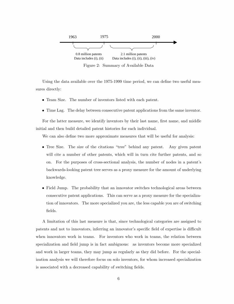
1963 1975 2000

0.8 million patentsData includes (i), (ii)

2.1 million patentsData includes (i), (ii), (iii), (iv)

Figure 2: Summary of Available Data

Using the data available over the 1975-1999 time period, we can de�ne two useful mea-

sures directly:

� Team Size. The number of inventors listed with each patent.

� Time Lag. The delay between consecutive patent applications from the same inventor.

For the latter measure, we identify inventors by their last name, �rst name, and middle

initial and then build detailed patent histories for each individual.

We can also de�ne two more approximate measures that will be useful for analysis:

� Tree Size. The size of the citations �tree� behind any patent. Any given patent

will cite a number of other patents, which will in turn cite further patents, and so

on. For the purposes of cross-sectional analysis, the number of nodes in a patent�s

backwards-looking patent tree serves as a proxy measure for the amount of underlying

knowledge.

� Field Jump. The probability that an innovator switches technological areas between

consecutive patent applications. This can serve as a proxy measure for the specializa-

tion of innovators. The more specialized you are, the less capable you are of switching

�elds.

A limitation of this last measure is that, since technological categories are assigned to

patents and not to innovators, inferring an innovator�s speci�c �eld of expertise is di¢ cult

when innovators work in teams. For inventors who work in teams, the relation between

specialization and �eld jump is in fact ambiguous: as inventors become more specialized

and work in larger teams, they may jump as regularly as they did before. For the special-

ization analysis we will therefore focus on solo inventors, for whom increased specialization

is associated with a decreased capability of switching �elds.

6

Finally, we would like to investigate the age at �rst innovation, as an outcome-based

measure that delineates the pre-innovation and active innovation phases. Unfortunately,

inventors�dates of birth are not available in the data set, nor from the USPTO generally.

However, using name and zip code information it was possible to attain birth date infor-

mation for a large subset of inventors through a public website, www.AnyBirthday.com.

AnyBirthday.com uses public records and contains birth date information for 135 million

Americans. The website requires a name and zip code to produce a match. Using a java

program to repeatedly query the website, it was found that, of the 224,152 inventors for

whom the patent data included a zip code, AnyBirthday.com produced a unique match in

56,281 cases. The age data subset and associated selection issues are discussed in detail in

the Data Appendix. The analysis there shows that the age subset is not a random sample

of the overall innovator population. This caveat should be kept in mind when examining

the age results, although it is mitigated by the fact that the di¤erences between the groups

become small when explained by other observables, controlling for these observables in the

age regressions has little e¤ect, and the results for team size and specialization persist when

looking in the age subset. See the discussion in the Data Appendix.

2.2 Time series results

I consider the evolution over time of our three outcomes of interest. Figure 1 presents the

basic data while Tables 2 through 4 examine the time trends in more detail.

Consider team size �rst. The lower right panel of Figure 1 shows that team size is

increasing at a rapid rate, rising from an average of 1.73 in 1975 to 2.33 at the end of

the period, for a 35% increase overall. Table 2 explores this trend further by performing

regressions relating team size to application year, and we see that the time trend is robust

to a number of controls. Controlling for compositional e¤ects shows that any trends into

certain technological categories or towards patents from abroad have little e¤ect. Repeating

the regressions separately for patents from domestic versus foreign sources shows that the

domestic trend is steeper, though team size is rising substantially regardless of source.

Repeating the time trend regression individually for each of the 36 di¤erent technological

categories de�ned by Hall et al. shows that the upward trend in team size is positive and

highly signi�cant in every single technological category. Running the regressions separately

by �assignee code�to control for the type of institution that owns the patent rights shows

7

that the upward trend also prevails in each of the seven ownership categories identi�ed

in the data, indicating that the trend is robust across corporate, government, and other

research settings, both in the U.S. and abroad.2 In short, we �nd an upward trend in team

size that is both general and steep.

Next consider the age at �rst innovation. Note that we de�ne an innovator�s ��rst�

innovation as the �rst time they appear in the data set. Since we cannot witness individuals�

patents before 1975, this de�nition is dubious for (i) older individuals, and (ii) observations

of ��rst� innovations that occur close to 1975. To deal with these two issues, I limit the

analysis to those people who appear for the �rst time in the data set between the ages of 25

and 35 and after 1985. The upper panel of Figure 1 plots the average age over time, where

we see a strong upward trend. The basic time trend in Table 3 shows an average increase

in age at a rate of 0.66 years per decade. Controlling for compositional biases due to shifts

in technological �elds or team size has no e¤ect on the estimates. The results are also

similar when looking at di¤erent age windows.3 Analysis of trends within technological

categories shows that the upward trend in age is quite general. Smaller sample sizes tend

to reduce signi�cance when the data is �nely cut, but an upward age trend is found in all

6 technology classes using Hall et al�s 6-category measure, and in 29 of 36 categories when

using their 36-category measure. The upward age trend also persists across all patent

ownership classi�cations.

Note that the age at �rst invention serves as an outcome-based measure to delineate

the education phase and innovation phase in the life-cycle. A possible contaminating factor

is the duration is takes to produce an innovation (the age at �rst invention is the sum of

age at completion of education plus the time lag until the �rst invention). However, in

results reported elsewhere (Jones 2005b), the time lags between an inventor�s inventions are

short, do not trend over time, and vary only modestly across �elds. Thus the age at �rst

invention appears to track the end of the educational phase with little error. Some related

evidence regarding doctoral duration is considered in Section 4.4

Now we turn to specialization. The specialization measure considers the probability

2Table A.2 describes the ownership assignment categories.3The table reports results for the 23 to 33 age window as well. In results not reported, I �nd that the

trend is similar across subsets of these windows: ages 23-28, 25-30, 31-35, et cetera. Furthermore, there isno upward trend when looking at age windows beginning at age 35.

4Doctoral age is also an imperfect delineation between education and innovation phases, because doctor-ates explicitly require innovative research that begins well before the awarding of the degree.

8

that an innovator switches �elds between consecutive innovations. Before looking at the

raw data, it is necessary to consider a truncation problem that may bias us toward �nding

increased specialization over time. The limited window of our observations (1975-1999)

means that the maximum possible time lag between consecutive patents by an innovator is

largest in 1975 and smallest in 1999. This introduces a downward bias over time in the

lag between innovations. It is intuitive, and it turns out in the data, that people are more

likely to jump �elds the longer they go between innovations.5 Mechanically shorter lags as

we move closer to 1999 can therefore produce an apparent increase in specialization. To

combat this problem, I make use of a conservative and transparent strategy. I restrict the

analysis to a subset of the data that contains only consecutive innovations which were made

within the same window of time. In particular, we will look only at consecutive innovations

when the second application comes within 3 years of the �rst. Furthermore, we will look

only at innovations which were granted within 3 years of the application.6 This strategy

eliminates the bias problem at the cost of limiting our data analysis to the 1975-1993 period

and making our results applicable only to the sub-sample of �faster�innovators.7 The lower

left panel of Figure 1 shows the trend from 1975-1993.

Table 4 considers the trend in specialization with and without this corrective strategy.

The results there, together with the graphical presentation in Figure 1, indicate a smooth

decrease in the probability of switching �elds. The decline is again quite steep. Using

the central estimate for the trend of -.003, we can interpret a 6% increase in specialization

every ten years. Note that our main results, and Figure 1, use the 414-category measure

for technology to determine whether a �eld switch has occurred. This is our most accurate

measure of technological �eld (Hall et al.�s measures are aggregations of it), but the results

are not in�uenced by the choice of �eld measure. Note in particular that the percentage

5An interpretation consistent with the spirit of the burden of knowledge concept is that people need timeto reeducate themselves when they jump �elds, hence a �eld jump is associated with a larger time lag.

6Looking only at patents where the second application came within 3 years limits our analysis to thosecases where the �rst application was made before 1997. However, a second issue is that patents are grantedwith a delay �2 years on average �and only patents that have been granted appear in the data. For a �rstpatent applied for in 1996, it is therefore much more likely that we will witness a second patent applied forin 1997 than one applied for in 1999 �introducing further downward bias in the data. To deal completelywith the truncation problem, we will therefore further limit ourselves to patents which were granted within3 years of their application, which means that we will only look at the period 1975-1993.

7These restrictions maintain a signi�cant percentage of the original sample. For example, of the 111,832people who applied successfully for patents in 1975, 81,955 of them received a second patent prior to 2000.Of these 81,955 people for whom we can witness a time lag between applications, 79.8% made their nextapplication within three years. Of those, 88.5% were granted both patents within three years of application.

9

trend is robust to the choice of the 6, 36, or 414 category measure for technology � the

trend is approximately 6% per decade for all three. Including controls for U.S. patents,

the application time lag, ownership status, and the technological class of the initial patent

has little e¤ect. Furthermore, looking for trends within each of Hall et al.�s 36 categories,

we �nd that the probability of switching �elds is declining in 34 of the 36; the decline is

statistically signi�cant in 20. In sum, we see a robust and strongly decreasing tendency for

solo innovators to switch �elds.

2.3 Cross-section results

For a �rst look at the data in cross-section, Table 5 presents a simple comparison of means

across the 6 and 36 technological categories of Hall et al (2001). The middle column

in the table presents the mean age at �rst innovation, and the data shows a remarkable

consistency across technological categories. In 31 of the 36 categories, an innovator�s �rst

innovation tends to come at age 29. The lowest mean age among the 36 categories is

28.8, and the highest - an outlier that relies on only 12 observations - is 31.1. The table

shows that regardless of whether the invention comes in �Nuclear & X-rays�, �Furniture,

House Fixtures�, �Organic Compounds�, or �Information Storage�, the mean age at �rst

innovation is nearly the same.8

The next columns of the table consider the average team size. Here we see large dif-

ferences across technological areas. The largest average team size, 2.91 for the �Drugs�

subcategory, is over twice that of the smallest, 1.41 for the �Amusement Devices�subcate-

gory.

Finally, the last columns of the table consider the probability that a solo innovator will

switch sub-categories between innovations. Here, as with team size and unlike the age at

�rst innovation, we see large di¤erences across technological areas. This variation is again

consistent with the predictions of the model. At the same time, this basic, cross-sectional

variation in the probability of �eld jump is di¢ cult to interpret: the probability of �eld

jump will be tied to how broadly a technological category happens to be de�ned, which

may vary to a large degree across categories.

8These results can also be considered in a regression format. Pooling cross-sections and using applicationyear dummies to take care of trends, the results are extremely similar. One can also adjust the time at �rstinnovation by subtracting category-speci�c estimates of the time lag to get a closer estimate of an individual�seducation. One can also look at di¤erent age windows. The result that ages are nearly identical across�elds is highly robust.

10

I can go further by using a direct measure of the quantity of knowledge underlying a

patent. In particular, I can analyze in cross-section what an increase in the knowledge

measure implies for our outcomes of interest.

For a continuous measure of the quantity of knowledge I will use the logarithm of the

number of nodes (i.e., patents) in the citation �tree� behind any patent.9 As before,

there is a truncation issue that needs to be considered: the data set does not contain

citation information for patents issued before 1975, so we tend to see the recent part of the

tree. The measure of underlying knowledge is then noisier the closer we are to 1975, and

I will therefore focus on cross-sections later in the time period. A second issue is that the

average tree size and its variance grow extremely rapidly in the time window, which makes it

di¢ cult to compare data across cross-sections without a normalized measure. Two obvious

normalizations are: (1) a dummy for whether the tree size is greater than the within-

period median; (2) the di¤erence from the within-period mean tree size, normalized by the

within-period standard deviation. Results are reported using the latter de�nition, as it is

informationally richer, though either method shows similar results.

Table 6 examines the relationship between team size and tree size in pooled cross-

sections, with and without various controls. I add a quadratic term for the variation in

team size to help capture evident curvature, and we see that team size rises at an increasing

rate as the measure of knowledge depth increases. For innovations with larger citation

trees, the rise in team size is particularly strong. With very deep knowledge trees, an

increase of one standard deviation in the tree size is associated with an average increase

in team size of one person. The table shows that the cross-sectional relationship holds

for domestic and foreign-source patents and when controlling for technological category, so

that the variation appears both within �elds and across them. Technological controls are

perhaps best left out, however, since the variations in mean tree size across technological

category may be equally of interest. Finally, we might be concerned that bigger teams

9The distribution of the raw node count within cross-section is highly skewed �the mean is far above themedian, so that upper tail outliers can dominate the analysis. I therefore use the natural log of the nodecount, which serves to contain the upper tail. A (loose) theoretical justi�cation is knowledge depreciation:distant layers of the tree are less relevant to a patent than nearer layers, so there is a natural diminishingimpact as nodes grow more distant. The diminishing impact of the large, distant layers, which dominatethe node counts, is captured loosely by taking logs. Noting that the basic results are similar when we usethe median-based measure of knowledge depth (a dummy for whether the raw node count is above or belowthe median, which is independent of any monotonic transform of the node count) we can be reasonablycomfortable with the log measure.

11

simply have a greater propensity to cite, which results in larger trees. This concern proves

unwarranted. Controlling for the variation in the direct citations made by each patent, we

�nd that relationship actually strengthens. In fact, we see that bigger teams tend to cite

less. This result gives us greater faith in the causative arrow implied by the regressions.

Next we turn to the age at �rst innovation. Table 7 examines, in pooled cross-sections,

the relationship between age and knowledge for those individuals for whom we can be

con�dent that they are innovating for the �rst time (see discussion above). The general

conclusion from the table is that we must work hard to �nd a relationship, and at its largest

it is very small. It is not robust to the speci�c age window, is reduced when controlling

for the technological category, and disappears when controlling for the number of direct

citations made. Taking a coe¢ cient of 0.1 as the maximum estimate from the table, we

�nd that an increase of one standard deviation in the knowledge measure leads to a 0.1

year increase in age. This coe¢ cient may be attenuated given that our proxy measure of

knowledge is noisy, but I conclude that there is at most only a weak relationship between

the amount of knowledge underlying a patent and the average age at �rst innovation.

Finally, Table 8 considers the relationship between the probability of �eld jump and

the knowledge measure. The table shows a robust negative relationship: solo innovators

are less likely to jump �elds when their initial patent has a larger node count. If we

identify a larger node count with a deeper area of knowledge, then this negative correlation

is consistent with the idea that deeper areas of knowledge see more specialization. The

results are robust to the inclusion of many controls, including controls for technological �eld,

foreign or domestic source of the patent, and the time lag between the two patents. The

results are also strengthened when looking at cross-sections later in the time period, where

the citations trees capture more historical information and may be less noisy measures of

the underlying knowledge.

To summarize, we have presented six facts about innovators. Using the measures

de�ned above, we �nd that specialization and teamwork appear to increase with time and

are also greater, in cross-section, in deeper areas of knowledge. Meanwhile, the average

age at �rst innovation is increasing with time, like specialization and teamwork, but shows

little variation with the depth of knowledge in cross-section. The following section presents

a model, building on the "burden of knowledge" idea, that (a) shows how these behaviors

can all emerge in equilibrium and (b) clari�es the growth implications. Further, related

12

evidence from existing literature will be discussion in Section 4.

3 The Model

The model considers innovator behavior along a balanced growth path. Building on foun-

dations of existing growth models, I analyze a structure with two sectors: a production

sector where competitive �rms produce a homogenous output good and an innovation sec-

tor where innovators produce productivity-enhancing ideas. The novelty of the model lies

in the innovators�choice problem. Innovators undertake costly human capital investments

to bring themselves to the knowledge frontier. Innovators weigh the costs and bene�ts of

gaining particular forms of expertise, decisions that will be balanced di¤erently by di¤erent

cohorts as the economy evolves and balanced di¤erently in di¤erent areas of application.

The model ties together the facts of Section 2 on the basis of these educational decisions

and shows how the burden of knowledge interacts with other forces in determining the

steady-state growth rate.

Section 3.1 describes the production sector and Section 3.2 de�nes individuals� life-

cycles and preferences. Sections 3.3 and 3.4 focus on innovators. The �rst describes the

knowledge space and the cost of education. The second considers the innovation process

and the value of ideas. Section 3.5 de�nes individuals�equilibrium choices, and Section

3.6 analyzes educational decisions and growth along a balanced growth path. Proofs are

presented in the Appendix.

3.1 The Production Sector

There is a continuum of productive ideas of measure N(t) > 0 at each time t 2 R. Let

each idea k 2 [0; N(t)] make a productivity contribution denoted (k) > 0. De�ne X(t) =R N(t)0 (k)dk as the collective productivity contribution of all existing ideas at time t.

Let there be a homogenous output good produced by competitive �rms at each time t.

The price of the good is normalized to 1 at each point in time. A �rm hires an amount of

labor, l(t), producing output y(t) = X(t)l(t) if all existing ideas k 2 [0; N(t)] are employed

by the �rm.10

10Firms use the whole set of existing ideas rather than just the latest idea. That is, we use a "horizontal"model of innovation, where ideas accumulate rather than become obsolete (see, e.g., Barro and Sala-i-Martin(1995) for a review).

13

Firms pay workers a competitive wage, w(t), and also make royalty payments. The

royalty payment per production worker is r(k; t) for idea k at time t, and the total royalty

payments per production worker are r(t) =R N(t)0 r(k; t)dk when all existing ideas k 2

[0; N(t)] are employed by the �rm. Pro�ts are �(t) = (X(t) � r(t) � w(t))l(t) when all

existing ideas are employed. Ideas receive patent protection for a �nite number of years

z > 0. It is straightforward to show that the monopolist owner of an unexpired patent

can charge a royalty per worker r (k; t) = (k) and competitive �rms will be just willing

to pay this fee.11 Meanwhile, r(k; t) = 0 for expired patents, which are freely available.

Hence �rms employ all available ideas, paying royalties on all unexpired patents totaling

r(t) = X(t)�X(t� z) per production worker. Total output in the economy is

Y (t) = X(t)LY (t) (1)

where LY (t) is the total mass of production workers. Competitive �rms earn zero pro�ts,

so that w(t) = X(t)� r(t), and the wage paid to a production worker is therefore

w(t) = X(t� z) (2)

3.2 Workers and Preferences

There is a continuum of workers of measure L(t) > 0 in the economy at time t. This

population grows at rate gL > 0. Individuals have a common hazard rate � of death.

Individuals are risk neutral, with expected utility for an individual i de�ned by

U i(�) =

Z 1

�ci(� ; t)e��(t��)dt (3)

where ci(� ; t) is the consumption at time t of an individual i born at time � .

I assume that individuals are born without assets and supply a unit of labor inelastically

at all points over their lifetime. Following standard models of �nite horizons (e.g. Blanchard

1985), we allow for competitive life insurance and annuity �rms so that loans are secured

11This production set-up follows closely on Arrow (1962) and Nordhaus (1969). The maximizationproblem of a �rm can be written explicitly as follows. De�ne eX(t) = R N(t)

0 (k)I(k; t)dk and er(t) =R N(t)

0r(k; t)I(k; t)dk where I(k; t) = 1 if the �rm employs idea k at time t and I(k; t) = 0 otherwise. The

�rm�s pro�t is e�(t) = ( eX(t) � er(t) � w(t))l(t) = (R N(t)0

[ (k)� r(k; t)] I(k; t)dk � w(t))l(t). To maximizepro�ts, the �rm chooses which ideas k to employ, setting I(k; t) = 1 when (k) � r(k; t) and I(k; t) = 0otherwise. The holder of a patent sets r(k; t) = (k) when the patent is valid, while r (k; t) = 0 when thepatent has expired. The �rm thus sets I(k; t) = 1 for all k 2 [0; N(t)]. Firms produce with productivityeX(t) = X(t), paying royalties on all unexpired patents totaling er(t) = X(t)�X(t� z) per worker.

14

by life insurance and assets held as annuities; thus workers do not die in debt or with

positive assets. In the absence of physical capital, the discount rate in this model is simply

�, the hazard rate of death.12 From the standard intertemporal budget constraint, the

individual�s utility is equivalent to the present value of her expected lifetime non-interest

income.

The individual maximizes lifetime income through the choice of career. This is a

permanent decision made at birth. In particular, the individual may become (i) a wage

worker or (ii) an innovator. Wage workers require no education, and the expected present

value of their lifetime income is the discounted �ow of the wage payments, w(t), they receive.

For a wage worker born at time � ,

Uwage (�) =

Z 1

�w(t)e��(t��)dt (4)

If an individual chooses to be an innovator, then she must further choose a speci�c �eld

of expertise, represented by a vector !i. The innovator pays an immediate educational cost

at birth, E(!i; �), to bring herself to the frontier of knowledge in the chosen �eld. She earns

an expected �ow of income, v(!i; t), throughout her life that comes from royalties on any

innovations she produces. The expected present value of lifetime income for an innovator

born at time � is

UR&D�!i; �

�=

Z 1

�v(!i; t)e��(t��)dt� E(!i; �) (5)

The structure of the innovator�s educational decision, !i, and the functional forms of

E(!i; �) and v(!i; t) are de�ned in the following subsections.

3.3 Knowledge and Education

Let knowledge be organized as follows. First, there are "areas of application". Second,

there is "foundational knowledge" underneath an area of application. For example, one

application area could be airplanes, building on foundational knowledge of �uid mechanics,

thermodynamics, and material science. Another application area could be drugs, build-

12The riskless rate of return is zero in the absence of physical capital; the discount rate exists purely tocover the possibility of death. In particular, the insurance premium to secure loans and the rate of return onannuities are both equivalent to the hazard rate of death under the zero-pro�t condition for insurance andannuity �rms. For example, an annuity �rm pays a stream � while you live in exchange for a dollar investedtoday. Expected pro�ts for the annuity �rm are 1� �=�. The zero pro�t condition then requires � = �.

15

ing on knowledge of immunology, protein synthesis, and bioinformatics. The amount of

foundational knowledge may di¤er for di¤erent areas of application.13

Formally, let there be J areas of application, indexed j 2 f1; 2; :::; Jg where J is �nite.

Within each area of application, there is a set of types of foundational knowledge arranged

around a circle of unit circumference. We denote each such circle �j and a point on such

a circle as sj . The measure of foundational knowledge in an application area is denoted

Dj(t), which one may visualize as in Figure 3. As helpful nomenclature, we will refer to

�j as a "circle of knowledge" and the measure Dj(t) the "depth of knowledge".

Figure 3: A �circle of knowledge�

A prospective innovator chooses an area of expertise, a vector ! = (j; sj ; bj) which de�nes

(1) an application area j 2 f1; 2:::; Jg; (2) a point, sj 2 �j , in the set of foundational

knowledge types underlying application area j; and (3) a certain distance, bj 2 [0;1),

measured clockwise of sj .14 To ease notation we have dropped the superscript i in the

vector !, and ask the reader to recall that ! is a choice made by an individual i.

For an innovator born at time � , the amount of knowledge the innovator acquires is the

individual�s chosen breadth of expertise, bj , multiplied by the prevailing depth of knowledge,

Dj(�). The educational cost of acquiring this information is:

E(!; �) = (bjDj(�))" (6)

13For simplicity, we assume that all areas of application are used in the production of the homogenousoutput good. One could alternatively allow for multiple types of output goods based on di¤erent areas ofapplication, but such an extension would distract from the core mechanism of the model and is thus leftaside.14We allow bj to take values greater than 1 - that is, for an innovator�s expertise to wrap around the

circle multiple times. One can imagine that innovators gain further educational value by covering the samefoundational knowledge again; e.g. re-reading material creates better understanding than one�s �rst read.This assumption is largely made for technical reasons, however, to avoid dealing with corner solutions wherechoices of bj are capped at some �nite maximum value. Corner solutions can be handled in a variation ofthe model, but are awkward and add no important insights.

16

where " > 0, which says that learning more requires a greater amount of education.

The depth of knowledge may di¤er across di¤erent application areas and may evolve

with time. In particular,

Dj(t) = DjX(t)� (7)

where Dj > 0 is speci�c to the application area. Thus the amount of foundational knowledge

for airplanes may be relatively large (high Dj) compared to amusement devices (low Dj).

With � > 0, the "depth of knowledge" increases over time as the productivity level of the

economy advances.

3.4 Innovation

Once educated, innovators begin to receive innovative ideas. The total stock of ideas at

time t is N(t). Let each idea (i.e. each unit mass of ideas) add to productivity by an

amount , so that productivity evolves as X(t) = N(t) when the total stock of ideas is

employed.15 Recalling that an idea can be licensed to LY (t) workers and patents last for

z years, the lump sum value of an idea is:

V (t) =

Z t+z

tLY (et)det (8)

Note that patents do not expire upon the death of an innovator.16 Like any asset, the

innovator prefers to hold a patent as an annuity, selling a patent to a competitive annuity

�rm in exchange for an annuity �V (t). For the innovator, the present value of this annuity

at time t is V (t).17

3.4.1 Inspiration

Ideas comes to an innovator at rate �(!; t). This arrival rate depends in part on an

innovator�s educational decision, !, which is �xed over an innovator�s lifetime, and in part

15One could alternatively allow the size of ideas to grow or decline with time, or allow the size of ideas tobe functions of educational choices. Such speci�cations would have no substantive e¤ect on the analysis.See Jones (2005b) and the discussion in Section 4.16This is a realistic feature of the model: in the real world patent rights are assignable and patents do

not expire on the death of an inventor.17 If the innovator did not have access to a competitive �nancial market that pays the innovator the lump-

sum value of the patent (or an equivalent annuity) in exchange for the patent rights, then the value of thepatent to the innovator would need to re�ect the possibility that the innovator dies before the patent rightsexpire, in which case V (t) =

R t+zt

LY (et)e��(et�t)det. This variation will have no impact on the main resultsof the model.

17

on the overall state of the economy, which evolves with time. In particular,

�(!; t) = AjX(t)�Lj(t; sj)

��b�j (9)

where Lj(t; sj) is the mass of living innovators at time t who have chosen location sj while

Aj represents application-area speci�c research opportunities.

This reduced-form speci�cation captures several key ideas. The parameter � repre-

sents the impact of the current state of technology on an innovator�s creative output. It

incorporates the standard ideas in the literature alluded to in the introduction: ��shing-

out�hypotheses whereby innovators�productivity falls as the state of knowledge advances

(� < 0), and rising technological opportunity whereby an improving state of knowledge

makes innovators more productive (� > 0). The term Aj > 0 meanwhile allows for techno-

logical opportunities to vary across application areas �for some areas to be relatively "hot"

or "cold".

The parameter � represents the impact of crowding on the frequency of an innovator�s

ideas. I assume 0 < � < 1, following standard arguments where innovators partly duplicate

each other�s work. A greater density of workers in the same specialty increases duplication,

reducing the rate at which a speci�c individual produces a novel idea.18

The �nal parameter, �, represents the impact of the breadth of expertise. We assume

� > 0, which says simply that broader foundational knowledge increases one�s productivity.

This is natural if, for example, access to a broader set of available knowledge �facts, theories,

methods �creates better combinatorial possibilities for one�s creativity, along the lines of

Weitzman (1998), making the innovator more productive.19

3.4.2 Implementation

Ideas are implemented by pooling requisite foundational knowledge. Implementation thus

involves the formation of teams. This process operates under simplifying assumptions as

follows.18An alternative formulation of (9), where individuals crowd over an interval of knowledge rather than a

point of knowledge, can explain the six stylized facts of Section 2 along the same lines as this model but isless tractable.19There are many other mechanisms through which broader expertise would enhance an innovator�s pro-

ductivity. For example, a more broadly expert innovator may better evaluate the expected impact andfeasibility of her ideas. She will better select toward high value, successful lines of inquiry, and thereforeachieve greater returns. Furthermore, if assembling teams is costly, innovators will be unwilling to formlarge teams. More broadly expert innovators can rely less on large teams for the implementation of theirideas, making their ideas less costly to implement.

18

First, it is assumed that implementation requires all types of foundational knowledge in

the given area of application. Formally, de�ne ideas in application area j as implementable

if for each sj 2 �j there exists an individual l in application area j such that sj lies in the

arc between slj and slj + b

lj . Let Ij(t) be an indicator function equal to 1 if the idea is

implementable and 0 otherwise.

Second, we assume that the innovator with the idea claims its rents. One may imagine

that innovators work in �rms, pooling knowledge in application area j, where the wage paid

to each innovative worker is the value of his ideas. Alternatively, one may think of the

innovator with an idea is a monopolist vis-a-vis potential teammates so that the inspired

innovator extracts all pro�ts from the project. We abstract from costs in team formation

or operation, so that all ideas are pro�table with lump-sum value V (t).

The expected �ow of income to an innovator, v(!; t), is then the probability an idea

arrives and is implementable times the lump-sum value of the idea.20 Hence

v(!; t) = �(!; t)Ij(t)V (t) (10)

Finally, we will consider below the size of teams. To simplify that analysis, we assume

an inspired innovator forms teams within her own cohort if possible and assembles the

minimum number of people necessary to implement the idea.

3.5 Equilibrium Career Choices

In equilibrium, a player cannot make a di¤erent choice of career and be better o¤. For an

individual born at any time � , the decision to become a wage worker requires that

Uwage (�) � UR&D�!0; �

�8!0

so that wage workers would not strictly prefer to be R&D workers. Similarly, for an

individual born at any time � the decision to become an R&D worker with educational20One can also consider rent-sharing among teammates, which adds considerable complexity. With rent-

sharing, equilibrium income �ow will still take the form of (10). This follows because innovators in thesame cohort earn the same income in equilibrium, which must then be the per-capita rate of idea arrivaltimes the value of ideas. At the same time, rent-sharing can create an ine¢ ciency should innovators expandtheir expertise not only to improve their creative output but also to claim greater royalty shares from theirteammates. While rent-sharing can thus a¤ect the bene�ts of breadth, the basic idea that the burden ofknowledge raises the cost of breadth, provoking increased specialization and teamwork, will be robust undera wide variety of rent-sharing arrangements. One might also consider many other possible frictions andine¢ ciencies in team formation. The model featured imagines that such frictions and incentive issues aresolved, allowing us to focus on a benchmark outcome. Also, see Jones (2008) for a model that features theintersection between educational decisions and frictions in team formation.

19

choice ! requires that

UR&D (!; �) � UR&D�!0; �

�8!0

UR&D (!; �) � Uwage (�)

so that R&D workers of type ! would not strictly prefer to be R&D workers of a di¤erent

type or wage workers.

3.5.1 Balanced Growth Path

We will focus on equilibrium career decisions along a balanced growth path. A balanced

growth path is de�ned such that the growth rate in productivity, g = _X(t)=X(t), is constant

over time and the labor allocations LY (t) and Lj(t; s) 8j; s grow with time at the population

growth rate gL. The existence of a balanced growth path will be established in the analysis

below.

We analyze the balanced growth path under three parametric restrictions that will be

assumed throughout the following analysis.

Assumption 1 � < "

This assumption is necessary for an innovator�s optimal breadth of expertise, the choice

bj , to be an interior maximum.

Assumption 2 �� �(� � 1" ) < 1

This assumption is necessary for the existence of a constant productivity growth rate g.

Assumption 3 � > max�g;�1 + �(� � 1

" )�g, where g = 1��

1��+�(�� 1")gL

This assumption is necessary for an individual�s lifetime income to be �nite.21

3.6 Analysis

Production workers receive a competitive wage w(t) = X(t � z) as shown in (2). Along

a balanced growth path, X(t � z) grows at rate g so that, from (4), a production worker

earns lifetime income

Uwage (�) =X(� � z)�� g (11)

where we require � > g for �nite lifetime income.22

21The death rate � is the discount rate. One could add a pure rate of time preference to the model, inaddition to the death rate /�, which would raise the discount rate and allow lifetime income to be boundedunder higher growth rates.22 It is demonstrated in the proof of Proposition 2 (below) that �nite income for wage workers follows from

Assumption 3 along a balanced growth path.

20

The innovator, meanwhile, makes an educational choice to maximize lifetime income.

With the objective function (5) and the de�nitions in (6), (9), and (10), the innovator�s

problem is:

max!=(j;sj ;bj)

Z 1

�AjX(t)

�Lj(t; sj)��b�j Ij(t)V (t)e

��(t��)dt� (bjDj(�))" (12)

The �rst result regarding career choice establishes the useful property of income equiv-

alence between innovators and wage workers.

Lemma 1 Along a balanced growth path UR&D(!; �) = Uwage(�) for any equilibrium choice

! and any cohort �

This income equivalence result rules out corner solutions where all individuals choose

to be wage workers or all choose to be innovators. It follows naturally in the set-up of the

model. Wage workers are needed to create a market for innovations, and innovators are

too productive when rare to fail to exist. Along a balanced growth path, masses of wage

workers and innovators are all growing, so that individuals actively choose both broad types

of careers in every cohort, and hence their income must be equivalent in equilibrium.

The next results further de�ne innovator behavior, building on the choice of ! =

(j; sj ; bj).

Proposition 1 Along a balanced growth path

i. Ij(t) = 1 for all j; t

ii. Lj(t; s0) = Lj(t; s00) for all s0; s00 in an area of application j

iii. E(!; �)=UR&D(!; �) = �"�� where � < "

Result (i) says that innovators exist with su¢ cient expertise to implement any idea in

any application area. This follows because duplication is costly so that innovators seek

to avoid crowding. In particular, with � > 0, any area of application with no active

innovators becomes too tempting to ignore � an innovator would always deviate to such

an area. Result (ii) follows from similar reasoning. It says that innovators spread evenly

within a given application area. This follows because, within an application area, there are

no costs or bene�ts of a particular location s except the relative density of innovators there.

Hence, with � > 0, innovators avoid crowding and array themselves evenly. For clarity,

we will denote the labor allocation Lj(t; s) as L�j (t) in equilibrium to emphasize that it is

21

independent of s in a given area of application j. The total mass of innovators at time t is

then L�R(t) =PJj=1 L

�j (t) and the total mass of wage workers is L

�Y (t) = L(t)� L�R(t).

Result (iii) is less obvious and more powerful. It says that the ratio between educational

expenditure and lifetime income is constant, regardless of the innovator cohort or particular

equilibrium area of expertise. This follows from the choice of bj , which equates the marginal

cost and bene�t of breadth. Generally, if we view Dj(�) as the �price�of breadth, then an

increased price results in decreased breadth, o¤setting the rise in total educational cost. In

this model, price and quantity are traded o¤ exactly so that educational cost is a constant

fraction of lifetime income. This type of result should be familiar from Cobb-Douglas

speci�cations, which feature constant expenditure shares.23 This result requires that a

choice bj represents an interior maximum, so that the marginal bene�ts and costs of breadth

are equated. This is guaranteed as long as � < " (Assumption 1) as shown in the Appendix.

Result (iii) is a key property of the equilibrium from which other results follow. As a

�rst example, recall that UR&D(!; �) = Uwage(�) in equilibrium, so that innovators�income

is independent of the particular equilibrium choice !. It then follows directly from result

(iii) that E(!; �) must likewise be independent of the particular equilibrium choice !. This

result is encapsulated as part of the following corollary.

Corollary 1 Total Education

i. (Cross-Section) E(!; �) = E(!0; �) for any two equilibrium choices !; !0 made by indi-

viduals in the same cohort �

ii. (Time-Series) E(!; �) grows across cohorts at rate gE = g

These results inform the two key empirical facts regarding educational attainment from

Section 2. Result (i) says that innovators in the same cohort choose the same amount of

education across di¤erent areas of application. What is particularly surprising is that this

result holds even though some areas may feature a greater di¢ culty in reaching the frontier

of knowledge (higher Dj) and some areas may be "hotter" than others, featuring more

innovative opportunities (higher Aj). This uniformity of education is possible through the

endogenous allocation of innovators to di¤erent careers. Innovators allocate themselves

across application areas to neutralize income di¤erences (and hence educational di¤erences)

23The technical basis for this type of result lies in isoelasticity. In particular, innovator output is isoelasticin breadth (just as output is isoleastic to the inputs in a Cobb-Douglas speci�cation). Isoelasticity drivesthe constant expenditure share.

22

using di¤erences in the degree of congestion to o¤set variation in technological opportunities

or educational burden.

Result (ii) follows directly along the balanced growth path, where income is growing at

rate g and hence education is too, maintaining a constant ratio as dictated by Proposition

1.iii. The model thus can match two key empirical facts of Section 2: common educational

attainment across widely di¤erent areas of application yet growing education over time.

Denote the common educational attainment E(!; �) within a cohort � as E�(�). This

equivalence of education in turn has direct implications for the breadth of expertise. Re-

arranging (6), we see that

bj = E(!; �)1="=Dj(�) (13)

Common E(!; �) = E�(�) within a cohort then implies the equilibrium breadth of expertise

will di¤er only by area of application j and cohort � . In particular, denoting the equilibrium

choice of breadth as b�j (�) and the growth rate in b�j (�) across successive cohorts as gb�j , we

�nd the following results.

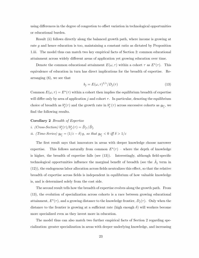
Corollary 2 Breadth of Expertise

i. (Cross-Section) b�j (�)=b�j0(�) = Dj0=Dj

ii. (Time-Series) gb�j = (1="� �) g, so that gb�j < 0 i¤ � > 1="

The �rst result says that innovators in areas with deeper knowledge choose narrower

expertise. This follows naturally from common E�(�) �where the depth of knowledge

is higher, the breadth of expertise falls (see (13)). Interestingly, although �eld-speci�c

technological opportunities in�uence the marginal bene�t of breadth (see the Aj term in

(12)), the endogenous labor allocation across �elds neutralizes this e¤ect, so that the relative

breadth of expertise across �elds is independent in equilibrium of how valuable knowledge

is, and is determined solely from the cost side.

The second result tells how the breadth of expertise evolves along the growth path. From

(13), the evolution of specialization across cohorts is a race between growing educational

attainment, E�(�), and a growing distance to the knowledge frontier, Dj(�). Only when the

distance to the frontier is growing at a su¢ cient rate (high enough �) will workers become

more specialized even as they invest more in education.

The model thus can also match two further empirical facts of Section 2 regarding spe-

cialization: greater specialization in areas with deeper underlying knowledge, and increasing

23

specialization over time. Moreover, increasing specialization - despite increasing educa-

tional attainment - is directly associated in the model with increasing depth of knowledge

along the growth path.

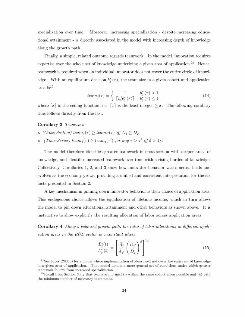
Finally, a simple, related outcome regards teamwork. In the model, innovation requires

expertise over the whole set of knowledge underlying a given area of application.24 Hence,

teamwork is required when an individual innovator does not cover the entire circle of knowl-

edge. With an equilibrium decision b�j (�), the team size in a given cohort and application

area is25

teamj(�) =

�1

d1=b�j (�)eb�j (�) > 1

b�j (�) � 1(14)

where dxe is the ceiling function; i.e. dxe is the least integer � x. The following corollary

thus follows directly from the last.

Corollary 3 Teamwork

i. (Cross-Section) teamj(�) � teamj0(�) i¤ Dj � Dj0

ii. (Time-Series) teamj(�) � teamj(�0) for any � > � 0 i¤ � > 1="

The model therefore identi�es greater teamwork in cross-section with deeper areas of

knowledge, and identi�es increased teamwork over time with a rising burden of knowledge.

Collectively, Corollaries 1, 2, and 3 show how innovator behavior varies across �elds and

evolves as the economy grows, providing a uni�ed and consistent interpretation for the six

facts presented in Section 2.

A key mechanism in pinning down innovator behavior is their choice of application area.

This endogenous choice allows the equalization of lifetime income, which in turn allows

the model to pin down educational attainment and other behaviors as shown above. It is

instructive to show explicitly the resulting allocation of labor across application areas.

Corollary 4 Along a balanced growth path, the ratio of labor allocations in di¤erent appli-

cation areas in the R&D sector is a constant where

L�j (t)

L�j0(t)=

24 AjAj0

Dj0

Dj

!�351=� (15)

24See Jones (2005b) for a model where implementation of ideas need not cover the entire set of knowledgein a given area of application. That model details a more general set of conditions under which greaterteamwork follows from increased specialization.25Recall from Section 3.4.2 that teams are formed (i) within the same cohort when possible and (ii) with

the minimum number of necessary teammates.

24

We see that innovators are attracted to "hot" application areas (high Aj) and areas with

low learning costs (low Dj). The interesting consequence is that while choice of application

area is in�uenced by these cross-�eld variations, educational attainment does not vary

across areas (Corollary 1). Meanwhile, breadth of expertise does vary with knowledge

depth (Corollary 2). The endogenous labor allocation thus helps neutralize educational

attainment but not specialization, allowing the model to unify the facts of Section 2.

3.6.1 Steady-State Growth

We now consider the implications of the knowledge burden mechanism for aggregate growth.

Growth comes from the summation of contributions from all innovators alive at a given

moment. If there are L�R(t) innovators active in equilibrium at time t and these innovators

raise productivity in the economy on average at rate ��(t), then productivity increases per

unit of time are simply _X(t) = ��(t)L�R(t). The growth rate of productivity is then

g =��(t)L�R(t)

X(t)(16)

Calculating innovators�average contributions, ��(t), appears complicated because inno-

vators are active in di¤erent areas of application with unique innovative opportunities and

knowledge depth, and innovators come from di¤erent cohorts. However, aggregating in-

novators�contributions is simpli�ed by the following result. In equilibrium, innovators in

the same cohort add to productivity at the same rate, regardless of their area of applica-

tion. The intuition builds from the results above: once individuals in the same cohort have

equivalent UR&D(!; �) and equivalent E(!; �) in equilibrium, their expected gross income

(UR&D(!; �) + E(!; �)) from innovation and hence their productivity contributions must

also be equivalent. This property, which is shown formally in the proof of the following

proposition, allows g to be determined as a simple function of exogenous parameters.

Proposition 2 Along a balanced growth path,

g =1� �

1� �+ �(� � 1" )gL (17)

where � � �(� � 1" ) < 1. There is a unique balanced growth path in equilibrium, with the

constant growth rate g given in (17) and a set of labor allocations fL�1(t); :::; L�J(t); L�Y (t)g

where each labor allocation grows at rate gL.

25

The expression (17) de�nes the growth rate as the outcome of several important forces,

marrying the knowledge burden mechanism with several ideas in the existing growth liter-

ature. First, the parameter �, as discussed above, represents standard ideas in the growth

literature whereby the productivity of innovators may increase as they gain access to new

technologies and new ideas (� > 0) or decrease if innovators are "�shing out" ideas (� < 0).

The larger � - the greater the value of knowledge to further innovation - the greater the

growth rate, as is seen in (17).

Second, the term �(� � 1" ) captures the implications of the burden of knowledge. The

term�� � 1

"

�is recognized from Corollary 2. With � > 1=" innovators choose increasing

specialization as the economy evolves, and we witness the �death of the Renaissance Man�

along the growth path . The impact of narrowing expertise on growth will be large or

small depending on the value of �, which de�nes the sensitivity of innovators�productivity

to their breadth of expertise.26

Expression (17) also shows that the model eliminates scale e¤ects. The productivity

growth rate is constant despite an exponentially increasing scale of research e¤ort, with the

number of researchers growing at the population growth rate, gL. In the model, growing

population provides both the motive �increasing market size �and the means - more minds

- for innovative e¤ort to grow at an exponential rate in equilibrium, even if innovation is

getting harder per person.

From a growth point of view, the burden of knowledge parameters �(�� 1" ) are seen to act

similarly in (17) to the parameter � that captures any �shing out e¤ect. Two interpretations

of the burden of knowledge mechanism are then possible. First, the �burden of knowledge�

mechanism can be seen as a micro-foundation for �shing-out type e¤ects on growth without

literally believing that ideas are being �shed out. Alternatively, if one is convinced that

a �shing-out process operates independently, then the burden of knowledge can be seen

as an additional e¤ect constraining the growth rate. Articulated views of why innovation

may be getting harder in the growth literature (Kortum 1997, Segerstrom 1998) and the

innovation literature (e.g. Evenson 1991, Henderson and Cockburn, 1996) have focused

on a "�shing out" idea. This paper o¤ers the burden of knowledge as a mechanism that

26 In a model with a time cost for education, an increasing burden of knowledge is also felt through increasededucational time, as this reduces the portion of the life-cycle left over to actively pursue innovations. Jones(2005b) considers this more general model.

26

makes innovation harder and acts similarly on the growth rate, thus explaining aggregate

data trends in addition to the micro facts presented in this paper.

4 Discussion

This paper is built on two observations. First, innovators are not born at the frontier of

knowledge but must initially undertake signi�cant education. Second, the distance to the

frontier may vary across �elds and over time. Motivated by these observations, I present

six novel facts about innovation in cross-section and time-series and a model that ties these

facts together.

The "burden of knowledge" mechanism can further inform several related facts in ex-

isting literature. First, consider �rst the age at �rst invention. Age at �rst invention is

an outcome-based measure intended to delineate the pre-innovation and innovation phases

in the life-cycle. Alternatively, one might consult an institutionally-based measure, such as

the age at highest degree. Existing evidence based on doctoral age also suggests an aging

phenomenon. Doctoral age rose generally across all major �elds from 1967-1986, with the

increase explained by longer periods in the doctoral program (National Research Council

1990). The duration of doctorates as well as the frequency of post-doctorates has been

rising across the life-sciences since the 1960s (Tilghman et al. 1998). Nobel Prize winners

also show a substantially increasing age at doctorate (Jones 2005a), as seen in Table 1.

The rise in teamwork also generalizes outside of patenting institutions, with similarly

broad trends reported in academic research. Increasing coauthorship in journal articles is

found in virtually all �elds of science, engineering, and the social sciences since the 1950s

(Wuchty et al. 2007). Studies of narrower samples of research �elds (e.g. Zuckerman and

Merton 1973) suggest that coauthorship has increased steadily since the early 20th century.

The model also provides an explicit analysis of growth, allowing it to inform aggregate

facts. In particular, an increasing burden of knowledge can explain why rapid growth in

the number of R&D workers and R&D dollars in the 20th century is not associated with

increased TFP growth rates or patenting rates (Machlup 1962, Evenson 1984, Kortum 1993,

Jones 1995b). The model thus provides a novel solution for the absence of �scale e¤ects�,

a much-debated subject in economic growth. At the same time, the model�s analysis of

growth is inclusive, incorporating existing mechanisms in the literature regarding innovation

27

exhaustion ("�shing out" stories), increasing innovation potential, and market size e¤ects.

We see explicitly that the burden of knowledge parameters enter the steady-state growth rate

equation much as the parameter capturing any �shing out e¤ect. Therefore, from a growth

perspective, one may view the �burden of knowledge�mechanism as a micro-foundation for

�shing-out type e¤ects, or, if one imagines a �shing-out process that operates independently,

then we can conceive of the burden of knowledge as an additional e¤ect constraining the

growth rate.

The model operates with several simpli�cations to focus on the central mechanisms,

but several generalizations are possible. For example, we focus on educational outlays

rather than educational duration per se; however, educational duration can be incorporated

explicitly in a more complex model and the predictions for innovator behavior remain the

same.27 The model also places the burden of knowledge mechanism in the rate of idea

production and assumes that the size of ideas is �xed. More generally, one may imagine

that the burden of knowledge is felt on the size of ideas rather than their rate, or on both

dimensions. This generalization is straightforward (see Jones 2005b) with no e¤ect on the

main propositions and corollaries.

In all, the micro-evidence presented in this paper, together with other available micro-

evidence and the aggregate data trends cited above, suggest general and multi-dimensional

patterns that may collectively be understood from the knowledge burden perspective. While

any individual piece of evidence can be explained by other means, the burden of knowledge

knits together a range of evidence within a single framework. Motivated by the burden

of knowledge concept, we are led to a set of striking facts, suggesting large changes in

the organization of innovative activity and providing a novel explanation for the absence

of �scale e¤ects� in growth. Moreover, the micro-evidence suggests that the burden of

knowledge is increasing. Note that, in general, a combination of increasing specialization

and increasing educational attainment is di¢ cult to reconcile without appealing to a greater

knowledge burden. If the distance to the frontier were not increasing, then increasing

education should be associated with broader individual knowledge, not narrowing expertise.

If a rising burden of knowledge is an inevitable by-product of technological progress,

27 Including time costs of education produces the same micro-econometric predictions but also introducesa second dimension through which the burden of knowledge in�uences growth. As equilibrium educationalduration increases along the growth path, the portion of an innovator�s life-cycle devoted to innovationdeclines, further restricting the growth rate. This is shown formally in Jones (2005b).

28

then ever-increasing e¤ort may be needed to sustain long-run growth. However, two kinds

of escapes are worth noting. First, if technological opportunities rise su¢ ciently rapidly,

then the output of innovators may become su¢ cient, despite a rising educational burden,

to sustain growth without increasing e¤ort. While the 20th century�s aggregate data pat-

terns - rapidly increasing R&D e¤ort but �at TFP growth - do not suggest a su¢ cient

rise in technological opportunity, there is nothing to say that su¢ ciently rapid avenues of

opportunity may not open in the future.

Second, even if the stock of knowledge accumulates over long periods, some future

revolution in science may simplify the knowledge space, causing a fall in the burden of

knowledge. Scienti�c revolutions �Kuhnian "paradigm" shifts (Kuhn 1962) �might there-

fore have signi�cant bene�ts by easing the inter-generational transmission of knowledge.

Related to this point, the e¢ ciency of education �the rate at which we transfer knowledge

from one generation to the next �becomes a policy parameter with �rst-order implications

for the organization of innovative activity and for growth. Future improvements in knowl-

edge transfer rates could potentially overcome growth in the knowledge stock. While this

transfer rate probably faces physiological limits, policy choices in education take on further

importance, as policy features from teacher pay to curricular design and the need for a

�liberal arts�education all impact the rate at which human capital can be transferred to the

young.

29

5 Appendix

Proof of Lemma 1I �rst show that, along a balanced growth path, LY (t) > 0 8t and Lj(t; sj) > 0 8 j, sj ,

t. I then show that this implies UR&D(!; �) = Uwage(�) for any equilibrium choice ! andcohort � .

1. LY (t) > 0 8t. By contradiction, let LY (t) = 0 for some t. On a balanced growthpath, where labor allocations grow at rate gL, LY (t) = 0 for some t implies LY (t) = 0

for all t. Furthermore, all workers must then be innovators. But these innovators wouldearn zero income, since there is no market for any innovation, with the value of innovationsV (t) = 0 for all t if LY (t) = 0 for all t. Therefore, innovators would strictly prefer to bewage workers, earning strictly positive income as de�ned by (4) with w(t) = X(t� z) > 0.Hence, by contradiction, LY (t) > 0 8t.

2. Lj(t; sj) > 0 8j, sj , t. By contradiction, let Lj(t; sj) = 0 for some j, sj and t, whichimplies that Lj(t; sj) = 0 for all t along a balanced growth path. This can�t hold becausebeing a scarce innovator is too tempting. Recalling that LY (t) > 0 in any equilibrium, sothere is a market for innovations, from the objective function (12), the choice j; sj ; bj = 1would produce unbounded income. This follows because the choice bj = 1 makes ideasimplementable and yet Lj(t; sj) = 0, which makes the rate of idea production unbounded.Hence a wage worker, who earns bounded income by (11) and Assumption 3, would preferto be such a scarce innovator. Hence, by contradiction, Lj(t; sj) > 0 8 j, sj , t.

3. Along a balanced growth path, labor allocations grow at rate gL. Hence LY (t) > 0implies that individuals in every cohort choose to become wage workers. Meanwhile,Lj(t; sj) > 0 implies that individuals in every cohort choose to be innovators. By theequilibrium conditions of Section 3.5 each choice is weakly preferred to any other andtherefore

UR&D(!; �) = Uwage(�)

for any equilibrium choice ! and cohort � .

Proof of Proposition 1.iAs shown in the proof of Lemma 1, Lj(t; sj) > 0 8j; sj ; t. Morever, bj > 0 since

otherwise individuals would earn zero income and could do better by choosing to be aproduction worker, who earns strictly positive income as shown in the proof of Lemma 1.Since individuals exist at every point sj and bj > 0 in any equilibrium, expertise exists atevery point on the circle and all ideas are implementable. Thus Ij(t) = 1 8j; t.

Proof of Proposition 1.iiBy contradiction, imagine that

Lj(t; s0) > Lj(t; s

00)

for two points s0 and s00 and some time t. Along a balanced growth path, Lj(t; s) must growat the population growth rate for any s, which implies that the ratio Lj(t; s0)=Lj(t; s00) isconstant and therefore Lj(t; s0) > Lj(t; s00) for all t if Lj(t; s0) > Lj(t; s00) for some t. Butthen anyone located at s0 would be strictly better o¤ if they had chosen s00. In particular,

30

the objective function (12) implies that UR&D (j; s0; b; �) < UR&D (j; s00; b; �) for a personborn at time � . (Given your choice of b, you would always prefer to be at the less crowdedlocation to avoid congestion.) Thus s0 would never be chosen in equilibrium. Thereforethere can be no points on the circle where the mass is less than any other point along abalanced growth path.

Proof of Proposition 1.iiiDi¤erentiating the innovator�s objective function, (12), with respect to bj , produces the

�rst order condition:

�

bj

Z 1

�AjX(t)

�L�j (t)��b�j V (t)e

��(t��)dt ="

bj(bjDj(�))

" (18)

where we have used Proposition 1.i and Proposition 1.ii to simplify the objective function;namely, Ij(t) = 1 8 j; t and Lj(t; s) is invariant with s in equilibrium and written L�j (t).

This �rst order condition is directly rewritten as �R1� v(!; t)e��(t��)dt = "E(!; �).

Noting from (5) thatR1� v(!; t)e��(t��)dt = UR&D (!; �)+E(!; �), the �rst order condition

is equivalentlyE (!; �) =UR&D (!; �) = �= ("� �) (19)

which is a constant.The second order condition takes the form @2UR&D=@b2j = �(� � 1)�

UR&D (!; �) + E(!; �)�=b2j � "("� 1)E(!; �)=b2j . The �rst order condition thus de�nes a

maximum under Assumption 1:� < "

which guarantees @2UR&D=@b2j < 0 where the �rst-order condition (19) holds.Note that we may also write the optimal choice bj as follows. Using (19), the de�nitions

of E (!; �) and Dj(�) in (6) and (7), and the property that UR&D (!; �) = Uwage (�) inequilibrium, where Uwage (�) = X(�)e�gz= (�� g), we have

b�j (�) =X(�)1="��

Dj

���

"� �

��e�gz

�� g

��1="(20)

where we write the optimal choice of bj as b�j (�) to clarify that in equilibrium breadthchoices depend on the application area j and cohort of birth � . Note that � < " followsfrom Assumption 1 and � > g by Assumption 3, so that b�j (�) is strictly positive. It is alsounique given area of application j and cohort � .

Proof of Corollary 1.i (Total Education, cross-section)By Lemma 1, income arbitrage implies UR&D (!; �) = UR&D (!0; �) for any equilibrium

choices !; !0 within a given cohort � . Since E(!; �)=UR&D (!; �) is a constant (Proposition1.iii), E(!; �) = E(!0; �) for any equilibrium choices !; !0 within a cohort � .

Proof of Corollary 1.ii (Total Education, time-series)By Proposition 1.iii, E(!; �)=UR&D (!; �) is constant. Hence E(!; �) grows at the same

rate as UR&D (!; �) across successive cohorts. From (11), gU = g. Therefore, gE = g.

31

Proof of Corollary 2.i (Breadth of Expertise, cross-section)From (6), bj = E(!; �)1="=Dj(�). By Corollary 1.i, all innovators in cohort � have

identical E(!; �) = E�(�) regardless of their equilibrium choice of !. Hence equilibriumchoices of bj di¤er only by cohort � and area of application j. Denoting equilibrium breadthof expertise as b�j (�), we see that b

�j (�)=b

�j0(�) = Dj0(�)=Dj(�). From (7), Dj(t) = DjX(t)

�,

and hence b�j (�)=b�j0(�) = Dj0=Dj .

28

Proof of Corollary 2.ii (Breadth of Expertise, time-series)Taking logs and di¤erentiating with respect to � , it follows from (13) that gb�j =

1"gE �

gDj . From Corollary 1.ii gE = g and from (7) gDj = �g. Therefore gb�j = (1" � �)g, so that

gb�j < 0 i¤ � > 1=".29

Proof of Corollary 3.i (Teamwork, cross-section)From (14), teamj(�) = d1=b�j (�)e if b�j (�) � 1 and teamj(�) = 1 otherwise. Hence

teamj(�) � teamj0(�) i¤ b�j (�) � b�j0 (�). From Corollary 2.i, b�j (�) � b�j0 (�) i¤ Dj � Dj0 .Therefore teamj(�) � teamj0(�) i¤ Dj � Dj0 .

Proof of Corollary 3.ii (Teamwork, time-series)From (14), teamj(�) = d1=b�j (�)e if b�j (�) � 1 and teamj(�) = 1 otherwise. Hence

teamj(�) � teamj(�0) i¤ b�j (�) � b�j (�

0). From Corollary 2.ii, b�j (�) is falling acrosscohorts i¤ � > 1=". Hence teamj(�) � teamj(�

0) for any � > � 0 i¤ � > 1=".

Proof of Corollary 4 (Labor Allocation)Consider the labor allocation across application areas within a given cohort of re-

searchers. Recalling from Proposition 1.iii that E (!; �) =UR&D (!; �) = �"�� , we can use the

de�nition of UR&D(!; �) in (5) to write UR&D(!; �) = "��"

R1� v(!; t)e��(t��)dt. Rewriting

v(!; t) using the de�nitions in (10) and (9) and the equilibrium properties of Proposition 1we have

UR&D(!; �) ="� �"AjX(�)

�b�j (�)�V (�)L�j (�)

��Z 1

�e�g(t��)e(1��)gL(t��)e��(t��)dt (21)

along a balanced growth path, so that UR&D(!; �) for a given cohort varies across appli-cations areas due only to di¤erences in L�j (�), Aj , and b

�j (�). Given that b�j (�)=b

�j0(�) =

Dj0=Dj (Corollary 2.i), the equilibrium condition UR&D(!; �) = UR&D(!0; �) is thereforesatis�ed by the labor allocation

L�j (�)

L�j0(�)=

24 AjAj0

Dj0

Dj

!�351=�

Proof of Proposition 2 (Steady-State Growth)

28This result may also be demonstrated directly using the expression for b�j (�) in (20) above.29See prior footnote.

32

To show (17) we proceed in three steps. First, it is shown that the rate at which aninnovator adds to productivity is the same in equilibrium for all innovators in the samecohort. Second, it is shown that the rate at which innovators add to productivity growsacross cohorts at a constant rate. Third, the steady-state growth rate of productivity isdetermined as the summation of contributions of active innovators.

1. Given common UR&D(!; �) and common E(!; �) for innovators in the same cohort� , it follows from the de�nition of UR&D(!; �) in (5) thatZ 1

�v(!; t)e��(t��)dt =

Z 1

�v(!0; t)e��(t��)dt (22)

Note further that v(!; t) grows with time t at a constant rate independent of !.30 Therefore(22) implies v(!; t) = v(!0; t) for individuals in the same cohort � at any point in time t.Writing v(!; t) = �(!; t)V (t), where we recall that �(!; t) is the rate of idea production,this in turn implies �(!; t) = �(!0; t) for individuals in the same cohort � at any point intime t.

Given this result, de�ne the common rate at which innovators in the same cohort addto productivity as ��(� ; t), where ��(� ; t) = �(!; t) for any equilibrium choice ! made attime of birth � . Noting the de�nition of �(!; t) in (9), in equilibrium we have

��(� ; t) = AjX(t)�L�j (t)

��b�j (�)� (23)

2. Inspecting (23), the productivity contributions of di¤erent cohorts di¤er only due totheir breadth of expertise, b�j (�). Further, given the results of Corollary 2.ii, b�j (�) growsacross cohorts at rate

�1" � �

�g and hence

��(� ; t) = ��(t; t)e�(1"��)g(��t) (24)

3. We can now aggregate the contributions of innovators alive at time t. This is theproductivity of each innovator cohort, weighted by the size of that cohort, summed over allliving cohorts. De�ning l�R(� ; t) as the mass of innovators who were born at time � whoremain alive at time t, we can write the average rate at which all living innovators add toproductivity as

��(t) =1

L�R(t)

Z t

�1��(� ; t)l�R(� ; t)d�

Noting that L�R(t) grows at rate gL and that innovators die at rate �, it is clear thatl�R(t; t) = (gL + �)L

�R(t) and l

�R(� ; t) = l

�R(t; t)e

(gL+�)(��t).31 Using these facts and (24) wehave

��(t) = ��(t; t)

Z t

�1(gL + �) e

�( 1"��)g(��t)e(gL+�)(��t)d� (25)

where the integral is a �nite constant if ��1" � �

�g + gL + � > 0, which is guaranteed by

Assumption 3, as discussed below.

30 In particular, v(!; t) = AjX(t)�Lj(t; s)��b�j V (t) is a collection of terms that are either constant given

! (Aj , bj) or growing at common rates independent of ! on a balanced growth path (X(t), Lj(t; s), V (t)).31The latter expression follows from two observations: (1) with death rate �, l�R(� ; t) = l

�R(� ; �)e

��(t��);(2) with growth rate gL, l�R(t; t) = l

�R(� ; �)e

gL(t��). Hence, l�R(� ; t) = l�R(t; t)e

(gL+�)(��t).

33

We are interested in the balanced growth path, where g is a positive constant. Recallfrom (16) that g = ��(t)L�R(t)=X(t). Taking logs in (16), di¤erentiating with respect totime, and asserting that g is a constant, we see that the steady-state growth rate is

g = g��(t) + gL�R(t)

Noting from (25) that g��(t) = g��(t;t) and, from (23), that g��(t;t) = �g � �gL + �gb�j , we�nd that g = �g + (1� �)gL + �

�1" � �

�g. Rearranging produces the unique steady-state

growth rate, the expression (17), repeated here

g =1� �

1� �+ �(� � 1" )gL

where �� �(� � 1" ) < 1 (Assumption 2).

Existence and uniqueness of balanced growth pathWe now con�rm that with the steady-state growth rate g de�ned in (17) there exists

a set of labor allocations fL�1(�); :::; L�J(�); L�Y (�)g each growing at rate gL that satis�esthe equilibrium conditions in Section 3.5; namely, that no individual would strictly pre-fer a di¤erent career choice. Moreover, we demonstrate that the set of labor allocationsfL�1(�); :::; L�J(�); L�Y (�)g, like the steady-growth rate above, is unique.32

We proceed in three steps. First, I con�rm that under Assumption 3 lifetime incomefrom di¤erent career choices is �nite - i.e. the integrals in (4) and (5) exist. Second, Idemonstrate the existence of a unique set of labor allocations fL�1(�); :::; L�J(�); L�Y (�)g on abalanced growth path such that in a particular cohort � no individual would strictly prefera di¤erent career choice. Finally, I con�rm that the equilibrium conditions are satis�ed inall cohorts along the balanced growth path where the steady-state growth rate g is as givenin (17).

1.The analysis has assumed that lifetime income, UR&D(!; �) and Uwage(�), is �nite.Having de�ned g explicitly along the balanced growth path, we can now state these as-sumptions as explicit parametric conditions. First, �nite lifetime income for a wage workerrequires � > g (see 11). Second, �nite income for an innovator requires � > �g+(1��)gL(see 21). With g given by (17), these conditions are satis�ed by Assumption 3. (Related,we assumed above that � > �

�� � 1

"

�g � gL so that the average productivity of innovators

is �nite (see 25). It is easy to show that this condition is also satis�ed by Assumption 3.)2. I now show that, given a steady-state growth rate g, there exists a unique set of

labor allocations fL�1(�); :::; L�J(�); L�Y (�)g for which individuals born at time � do notstrictly prefer another career choice. Note �rst that Corollary 4 established labor ratiosL�j (�)=L

�j0(�) such that U

R&D(!; �) = UR&D(!0; �) for any two equilibrium choices !, !0 incohort � . Hence innovators in the same cohort do not strictly prefer to be another type ofinnovator. This result depends on the labor ratios L�j (�)=L

�j0(�) and not on the overall scale

of research, L�R(�). We can then set L�R(�), and hence L�Y (�) = L(�) � L�R(�), at some

unique value to ensure that neither wage workers nor innovators strictly prefer a di¤erentcareer. This is clear because innovator income strictly, continuously decreases over the

32That is, the measures of workers are unique; the equilibrium does not uniquely assign particular indi-viduals to particular careers.

34

entire positive real line as L�R(�) increases while wage worker income is a �nite constant.33

This unique L�R(�) pins down L�j (�) for all j and also pins down L

�Y (t) = L(t) � L�R(t).

Hence there exists a unique set of equilibrium labor allocations fL�1(�); :::; L�J(�); L�Y (�)gfor which no individual born at time � would prefer a di¤erent career choice.

3. We have established the existence of a unique set of labor allocations such thatUR&D(!; �) = Uwage(�) for any equilibrium choice ! in a particular cohort � . From (11),Uwage(�) grows across cohorts at steady-state rate g. Hence equilibrium will be satis�edin all cohorts if UR&D(!; �) also grows at rate g across cohorts. Taking logs of (21),di¤erentiating with respect to � , and setting equal to g gives g = �g+�(1" � �)g+gL��gL.Rearranging this expression reproduces (17). Hence, the balanced growth path satis�es theconditions for equilibrium. The steady state growth rate is as given in (17), with the laborallocations fL�1(t); :::; L�J(t); L�Y (t)g each growing at rate gL.34

6 Data Appendix

The reader is referred to Hall et al. (2001) for a detailed discussion of their patent data set.This appendix focuses on the age information collected to augment the Hall et al. data.

Age data was collected using the website www.AnyBirthday.com, which requires a nameand zip code to produce a match. As is seen in Table A.1, 30% of U.S. inventors listed a zipcode on at least one of their patent applications, and of these inventors AnyBirthday.comproduced a birth date in 25% of the cases. While the number of observations producedby AnyBirthday.com is large, it represents only 7.5% of U.S. inventors. This Appendixexplores the causes and implications of this selection. The �rst question is why zip codeinformation is available for only certain inventors. The second question is why AnyBirth-day.com produces a match only one-quarter of the time. The third question is whether

33This can be seen formally as follows. Use (15) to write L�k(t) =�AkAj

�Dj

Dk

���1=�L�j (t). Noting that

L�R(t) =PJ

j=1 L�j (t), we can sum across areas of application to write L�R(t) = L

�j (t)

PJk=1

�AkAj

�Dj

Dk

���1=�,

or L�j (�) = cL�R(�) where c =

PJk=1

�AkAj

�Dj

Dk

���1=�!�1is a constant. Substituting L�j (�) = cL

�R(�) into

(21), we see that UR&D(!; �) is continuous and monotonically decreasing in L�R(�). This follows becauseincreasing L�R(�) (a) increases crowding (L

�j (�)

�� falls) and (b) reduces the market size for innovations (L�Y (t)falls and hence V (t) falls), both of which reduce UR&D(!; �). Moreover, limL�

R(t)!0+ U

R&D(!; �) =1 and

limL�R(t)!L(t)� U

R&D(!; �) = 0. Hence, we can pick some L�R(�) 2 [0; L(�)] such that UR&D(!; �) is anypositive value. Meanwhile, Uwage(�) is a �nite, strictly positive constant. Hence there exists some uniquescale of research activity, L�R(�); such that U

R&D(!; �) = Uwage(�) in the cohort born at time � .34Note that the growth rate, g, is determined two alternative ways. The �rst approach considers the

steady-state growth rate as the summation of contributions of innovators. The second approach considersthe steady-state growth rate that guarantees the equilibrium condition UR&D(!; �) = Uwage(�) will holdacross cohorts. It is instructive to clarify why these two methods produce the same result. First, innovators�total productivity contributions follow the evolution of ��(t), their average rate of productivity contributionsper innovator, and L�R(t), the scale of research e¤ort. Second, innovator income across cohorts follows theevolution of �(t; t) across cohorts and L�Y (t), the scale of the market. On the balanced growth path, L

�R(t)

and L�Y (t) grow at the same rate. Meanwhile, as shown above, the evolution of ��(t) with time and theevolution of �(t; t) from one cohort to the next are also equivalent. Hence, calculating growth from eitherperspective produces the same growth rate along a balanced growth path.

35

this selection appears to matter.Table A.2 compares how patent rights are assigned across samples. The table shows

clearly that zip code information is virtually always supplied when the inventor has yetto assign the rights; conversely, zip code information is never provided when the rightsare already assigned. Patent rights are usually assigned to private corporations (80% ofthe time) and remain unassigned in the majority of the other cases (17% of the time).An unassigned patent indicates only that the inventor(s) have not yet assigned the patentat the time it is granted. Presumably, innovators who provide zip codes are operatingoutside of binding contracts with corporations, universities, or other agencies that wouldautomatically acquire any patent rights. The zip-code subset is therefore not a randomsample, but is capturing a distinct subset of innovators who, at least at one point, wereoperating independently. Despite this distinction, this subset may not be substantiallydi¤erent from other innovators: the last column of Table A.2 indicates that, when lookingat the other patents produced by these innovators, they have a similar propensity to assignthem to corporations as the U.S. population average.

The nature of the selection introduced by AnyBirthday.com is more di¢ cult to iden-tify. The website reports a database of 135 million individuals and reports to have builtits database using �public records�. Access to public records is a contentious legal issue.35

Public disclosure of personal information is proscribed at the federal level by the Freedomof Information Act and Privacy Act of 1974. At the state and local level however, rulesvary. Birth date and address information are both available through motor vehicle depart-ments and their electronic databases are likely to be the main source of AnyBirthday.com�srecords.36 The availability of birth date information is therefore very likely to be relatedto local institutional rules regarding motor vehicle departments. Geography thus will in-�uence the presence of innovators in the age sample, and a further issue in selection mayinvolve the geographic mobility of the innovator, among other factors. The in�uence of thisselection, together with the implications of assignment status, can be assessed by comparingobservable means in the population across subsamples.

Table A.3 considers average team size, which is a source of further di¤erences. Patentswith provided zip codes have smaller team sizes than the U.S. average; team sizes in thesubset of these patents for which the age of one innovator is known are slightly larger, butstill smaller than the U.S. average. Controlling for other patent observables, in particularthe assignment status, reduces the mean di¤erences and brings the age sample quite closelyin line with the U.S. mean. (See the last two columns of the table.) Having examined anumber of other observables in the data, such as citations received and average tree size,I �nd that relatively small di¤erences tend to exist in the raw data, and that these canbe either entirely or largely explained by controlling for assignment status and team size.

35Repeated requests to AnyBirthday.com to de�ne their sources more explicitly have yet to produce aresponse.36A federal law, the Driver�s Privacy Protection Act of 1994, was introduced to give individuals increased

privacy. The law requires motor vehicle departments to receive explicit prior consent from an individualbefore disclosing their personal information. However, the law makes an exception for cases where motorvehicles departments provide information to survey and marketing organizations. In that case, individual�sconsent is assumed unless the individual has opted-out on their own initiative. See Gellman (1995) for anin-depth discussion of the laws and legal history surrounding public records.

36

Most importantly, the age results in the text are all robust to the inclusion of assignmentstatus, team size, and any other available controls.

Finally, looking at team size, specialization, and time lag trends in the age subsample,the results are similar in sign and signi�cance as those presented in Section 4. The rate ofincrease in specialization is larger, and the rate of increase in team size is smaller. The timelag shows no trend. Reexamining trends in the entire data set by assignment status, I �ndthat the team size trend is weaker among the unassigned category, which likely explains theweaker trend in the age subset. Similarly, I �nd that the specialization trend is strongeramong the unassigned category, which likely explains the stronger trend in the age subset.

I conclude therefore that while the age subset is not a random sample of the U.S.innovator population, the di¤erences tend to be explainable with other observables and, onthe basis of including such observables in the analysis, the age results appear robust.

References

[1] Aghion, Philippe and Howitt, Peter. �A Model of Growth through Creative Destruc-tion,�Econometrica, March 1992, 60, 323-351.

[2] Arrow, Kenneth J. �Economic Welfare and the Allocation of Resources for Invention,�in Nelson, R., eds. The Rate and Direction of Inventive Activity: Economic and SocialFactors, Princeton, NJ: Princeton University Press, 1962, 609-625.

[3] Barro, Robert and Sali-i-Martin, Xavier. Economic Growth, New York, NY: McGrawHill, 1995.

[4] Ben-Porath, Yoram. �The Production of Human Capital and the Life Cycle of Earn-ings,�Journal of Political Economy, August 1967, 75, 352-365.

[5] Blanchard, Olivier J. �Debt, De�cits, and Finite Horizons,�Journal of Political Econ-omy, April 1985, 93, 223-247.

[6] Evenson, Robert E. �International Invention: Implications for Technology MarketAnalysis,�in Zvi Griliches, ed., R&D, Patents, and Productivity, Chicago, IL: Univer-sity of Chicago Press, 1984, 89-123.

[7] � � . "Patent Data by Industry: Evidence for Invention Potential Exhaustion?"Technology and Productivity: The Challenge for Economic Policy, 1991, Paris: OECD,233-248.

[8] Gellman, Robert. �Public Records: Access, Privacy, and Public Pol-icy,� Center for Democracy and Technology Discussion Paper, April 1995,http://www.cdt.org/privacy/pubrecs/pubrec.html.

[9] Hall, Bronwyn H., Ja¤e, Adam B., and Trajtenberg, Manuel. �The NBER PatentCitations Data File: Lessons, Insights and Methodological Tools,� NBER WorkingPaper No. 8498, October 2001.

[10] Hart, Oliver and Moore, John. �A Theory of Debt Based on the Inalienability ofHuman Capital,� Quarterly Journal of Economics, November 1994, 109, 841-879.

[11] Henderson, Rebecca and Cockburn, Iain. �Scale, Scope, and Spillovers: The Deter-minants of Research Productivity in Drug Discovery,� Rand Journal of Economics,Spring 1996, 27, 32-59.

37

[12] Jones, Benjamin F. �Age and Great Invention,�NBERWorking Paper #11359, 2005a.

[13] � � . �The Burden of Knowledge and the Death of the Renaissance Man: Is InnovationGetting Harder?�NBER Working Paper #11360, 2005b.

[14] � � . �The Knowledge Trap: Human Capital and Development, Reconsidered" North-western University mimeo, 2008.

[15] Jones, Charles I. �R&D-Based Models of Economic Growth,� Journal of PoliticalEconomy, August 1995a, 103, 759-784.

[16] � � . �Time Series Tests of Endogenous Growth Models,�Quarterly Journal of Eco-nomics, May 1995b, 110, 495-525.

[17] Kortum, Samuel S. �Equilibrium R&D and the Decline in the Patent-R&D Ratio:U.S. Evidence,�American Economic Review Papers and Proceedings, May 1993, 83,450-457.

[18] � � . �Research, Patenting, and Technological Change,� Econometrica, November1997, 65, 1389-1419.

[19] Kuhn, Thomas. The Structure of Scienti�c Revolutions, Chicago, IL: University ofChicago Press, 1962.

[20] Machlup, Fritz. The Production and Distribution of Knowledge in the United States,Princeton, NJ: Princeton University Press, 1962, 170-176.

[21] Malone, Michael S. The Microprocessor: A Biography, New York, NY: Springer-VerlagNew York, 1995.

[22] National Research Council, On Time to the Doctorate: A Study of the Lengthen-ing Time to Completion for Doctorates in Science and Engineering, Washington, DC:National Academy Press, 1990.

[23] Nordhaus, William D. �An Economic Thoery of Technological Change,� AmericanEconomic Review, May 1969, 59, 18-28.

[24] Romer, Paul M. �Endogenous Technological Change,�Journal of Political Economy,October 1990, 98, S71-S102.

[25] Scotchmer, Suzanne. "Standing on the Shoulders of Giants - Cumulative Research andPatent Law", Journal of Economic Perspectives, Winter 1991, 5, 29-41.

[26] Segerstrom, Paul. �Endogenous Growth Without Scale E¤ects,�American EconomicReview, December 1998, 88, 1290-1310.

[27] Tilghman, Shirley (chair) et al. Trends in the Early Careers of Life Sciences, Wash-ington, DC: National Academy Press, 1998.

[28] Weitzman, Martin L. �Recombinant Growth,�Quarterly Journal of Economics, May1998, 113, 331-360.

[29] Young, Alwyn. �Growth Without Scale E¤ects,�Journal of Political Economy, Feb-ruary 1998, 106, 41-63.

[30] Wuchty, Stefan, Jones, Benjamin F. and Uzzi, Brian. �The Increasing Dominance ofTeams in the Production of Knowledge,�Science, May 2007, 316, 1036-1039.

[31] Zuckerman, Harriet and Merton, Robert. �Age, Aging, and Age Structure in Science,�in Merton, Robert, The Sociology of Science, Chicago, IL: University of Chicago Press,1973, 497-559.

38

39

Table 1: Age Trends among Nobel Prize Winners

Dependent Variable:

Age at Great Achievement

Dependent Variable:

Age at Highest Degree

Year of Great

Achievement

(in 100’s)

5.83***

(1.37)

--

Year of

Highest Degree

(in 100’s)

-- 4.11

***

(0.61)

Number of

observations

544

505

Time span

1873-1998

1858-1990

Average age

38.6

26.5

R2

0.027

0.084

NOTES:

(i) This table borrows from Jones (2005a). Age trends are measured in

years per century. Standard errors are given in parentheses.

(ii) Nobel Prize winners include all winners in Physics, Chemistry,

Medicine, and Economics. Age at great achievement is age when

contribution is made (not later age when prize is awarded). ***

Indicates 99% confidence level.

40

Table 2: Trends in Inventors per Patent

Dependent Variable: Inventors per Patent

(1)

(2)

(3) (4) (5) (6) (7)

Application Year

.0293

(.0001)

.0261

(.0001)

.0262

(.0001)

.0251

(.0001)

.0244

(.0002)

.0306

(.0002)

.0180

(.0003)

Foreign Patent

--

.444

(.002)

.416

(.002)

.141

(.004)

.146

(.004)

US Only

Foreign

Only

Tec

hn

olo

gic

al

Fie

ld C

on

tro

ls

Broad

--

Yes

--

--

--

--

--

Narrow

--

--

Yes

Yes

Yes

Yes

Yes

Assignee Code

--

--

--

Yes

Yes

Yes

Yes

Number of

Observations

2,016,377

2,016,377

2,016,377

2,016,377

1,506,956

1,123,310

893,067

Period

1975-

1999

1975-

1999

1975-

1999

1975-

1999

1975-

1996

1975-

1999

1975-

1999

Mean of Dependent

Variable

2.03

2.03

2.03

2.03

1.97

1.82

2.29

Per-decade Trend as %

of Period Mean

14.4%

12.9%

12.9%

12.4%

12.4%

16.8%

7.9%

R2

.02

.08

.10

.12

.13

.12

.10

NOTES

(i) Regressions are OLS with standard errors in parentheses. Specifications (1) through (4) consider the entire

universe of patents applied for between 1975 and 1999. Specification (5) considers only patents that were granted

within three years after application (see discussion in text). Specifications (6) and (7) present separate trends for

domestic and foreign source patents.

(ii) Foreign Patent is a dummy variable to indicate whether the first inventor listed with the patent has an address

outside the U.S..

(iii) ―Broad‖ technological controls include dummies for each of the 6 categories in Hall et al.’s most aggregated

technological classification. ―Narrow‖ technological controls include dummies for each category of their 36-category

classification.

(iv) Upward trends persist when run separately for each technological field. Using the broad classification (six

categories), the trends range from a low of .018 for ―Other‖ to a high of .037 for ―Chemical‖. Using the narrower

classification scheme (thirty-six categories), the trends range from a low of .007 for ―Apparel &Textile‖ to .051 for

―Organic Compounds‖. The smallest t-statistic for any of these trends is 7.76.

(v) Assignee code controls are seven dummy variables that define who holds the rights to the patent. Most patent

rights are held by U.S. or foreign corporations (80%), while a minority remain unassigned (17%) at the time the patent

is issued. Table A.2 describes the assignee codes in further detail. Running the time trends separately for the

individual assignee codes shows that the team size trends range from a low of .005 for the unassigned category to a

high of .039 for US non-government institutions. The lowest t-statistic for any of these trends is 5.38.

41

Table 3: Trends in Age at First Innovation

Dependent Variable: Age at Application

(1)

(2)

(3) (4) (5) (6) (7)

Application Year

.0657

(.0095)

.0666

(.0095)

.0671

(.0095)

.0671

(.0099)

.0687

(.0097)

.0530

(.0107)

.0584

(.0109)

Tec

hn

olo

gic

al

Fie

ld C

on

tro

ls

Broad

--

Yes

--

--

--

--

--

Narrow

--

--

Yes

Yes

Yes

--

Yes

Assignee Code

--

--

--

Yes

Yes

--

Yes

Team Size

--

--

--

--

-.0630

(.0273)

--

-.0348

(.0306)

Number of observations

6,541

6,541

6,541

6,541

6,541

5,102

5,102

Period

1985-

1999

1985-

1999

1985-

1999

1985-

1999

1985-

1999

1985-

1999

1985-

1999

Age Range

25-35 25-35 25-35 25-35 25-35 23-33 23-33

Mean of Dependent

Variable

31.0

31.0

31.0

31.0

31.0

29.3

29.3

Per-decade Trend as %

of Period Mean

2.1%

2.1%

2.2%

2.2%

2.2%

1.8%

2.0%

R2

.007

.010

.020

.020

.021

.005

.018

NOTES

(i) Regressions are OLS, with standard errors in parentheses. All regressions look only at those innovators for whom

we have age data and who appear for the first time in the data set in or after 1985. Specifications (1) through (5)

consider those innovators who appear for the first time between ages 25 and 35. Specifications (6) and (7) consider

those innovators who appear for the first time between ages 23 and 33.

(ii) ―Broad‖ technological controls include dummies for each of the 6 categories in Hall et al.’s most aggregated

technological classification. ―Narrow‖ technological controls include dummies for each classification in their 36-

category measure. The upward age trend persists when run separately in each of Hall et al’s broad technology classes.

These trends are significant in 5 of the 6 categories, with similar trend coefficients as when the data are pooled.

Upward trends are also found in 29 of 36 categories when using Hall et al.’s narrow technology classification. Here

12 categories show significant upward trends. Sample sizes drop considerably when the data is divided into these 36

categories. The one case of a significant downward trend (category #23, Computer Peripherals) has 42 observations.

(iii) Assignee code controls are seven dummy variables that define who holds the rights to the patent. Table A.2

describes the assignee codes in further detail. The upward age trends persist when run separately for each assignee

code and are similar in magnitude to the trends in the table above.

42

Table 4: Trends in Probability of Field Jump

Dependent Variable: Probability of Switching Technological Field

(1)

414

(2)

414

(3)

36

(4)

36

(5)

6

(6)

6

(7)

414

(8)

414

Application Year

-3.4e-3

(.19e-3)

-3.2e-3

(.19e-3)

-2.5e-3

(.19e-3)

-2.8e-3

(.19e-3)

-1.9e-3

(.17e-3)

-2.3e-3

(.17e-3)

-5.1e-3

(.12e-3)

-3.0e-3

(.11e-3)

Foreign Patent

--

.0076

(.0039)

--

-.0041

(.0038)

--

.0002

(.0035)

--

-.0005

(.0029)

Time Between

Applications

--

.0225

(.0012)

--

.0206

(.0012)

--

.0154

(.0011)

--

.0228

(.0004)

Technological

Field Controls

(first patent)

--

Yes

--

Yes

--

Yes

--

Yes

Assignee Code

(first patent)

--

Yes

--

Yes

--

Yes

--

Yes

Number of

observations

215,855

215,855

215,855

215,855

215,855

215,855

359,405

359,405

Period

1975-

1993

1975-

1993

1975-

1993

1975-

1993

1975-

1993

1975-

1993

1975-

1999

1975-

1999

Mean of

Dependent

Variable

.535

.535

.423

.423

.294

.294

.556

.556

Per-decade

Trend as % of

Period Mean

-6.4%

-6.0%

-5.9%

-6.4%

-6.5%

-7.8%

-9.4%

-5.6%

(Pseudo) R2

.0011

.018

.0006

.019

.0005

.017

.004

.026

NOTES

(i) Results are for probit estimation, with coefficients reported at mean values and standard errors in parentheses. The

coefficient for the Foreign dummy is reported over the 0-1 range.

(ii) The dependent variable is 0 if an inventor does not switch fields between two consecutive innovations. The dependent

variable is 1 if the inventor does switch fields. Column headings define the field classification used to determine the

dependent variable: ―414‖ indicates the 414-category technological class definition of the USPTO; ―36‖ and ―6‖ refer to the

aggregated measures defined by Hall et al (2001).

(iii) Specifications (1) through (6) consider ―fast‖ innovators -- only those consecutive patents with no more than 3 years

between applications and with no more than 3 years delay between application and grant. (See discussion in text.)

Specifications (7) and (8) consider all consecutive patents.

(iv) Technological field controls are dummies for the 36 categories defined by Hall et al (2001). The reported regressions

use the technological field of the initial patent. Using the field of the second patent has no effect on the results. Running the

regressions separately by technology category shows that the trends persist in 6 of 6 categories using Hall et al.’s broad

technology classification and 34 of 36 categories using Hall et al’s narrow classification with significant trends in 20.

(v) Assignee code controls are seven dummy variables that define who holds the rights to the patent. Table A.2 describes the

assignee codes in further detail. The declining probability of field jump persists when the trend is examined within each

assignment code, although the significance of the trend disappears in the rarer classifications.

43

Table 5: Mean differences across Technological Categories

Technological Classification

(Hall et al. 2001)

Age at First

Innovation

Inventors per

Patent

Probability of

Field Jump

6 36 Code Obs Mean Obs Mean Obs Mean

Ch

emic

al (

1)

Agriculture, Food, Textiles 11 12 31.1 18,351 2.45 2,461 0.48

Coating 12 52 29.2 32,820 2.24 4,336 0.64

Gas 13 17 29.9 10,047 1.96 1,692 0.59

Organic Compounds 14 49 29.4 78,188 2.57 8,010 0.32

Resins 15 43 29.4 74,993 2.52 7,695 0.37

Miscellaneous—Chemical 19 329 29.3 214,854 2.23 29,721 0.43

Entire category 502 29.4 429,253 2.35 53,915 0.43

Co

mp

ute

rs &

Co

mm

un

icat

ion

s

(2)

Communications 21 270 29.2 98,046 1.99 15,107 0.41

Computer Hardware & Software 22 169 29.8 83,094 2.26 10,259 0.44

Computer Peripherals 23 38 29.2 22,809 2.37 2,772 0.51

Information Storage 24 45 29.0 43,182 2.21 6,778 0.40

Entire category 522 29.4 247,131 2.15 34,916 0.42

Dru

gs

&

Med

ical

(3

) Drugs 31 74 29.9 77,210 2.91 7,181 0.25

Surgery & Medical Instruments 32 276 29.8 62,192 1.86 12,385 0.29

Biotechnology 33 48 30.5 29,638 2.75 2,223 0.36

Misc—Drugs & Medical 39 71 29.2 14,356 1.66 3,488 0.35

Entire category 469 29.8 183,396 2.43 25,277 0.29

Ele

ctri

cal

&

Ele

ctro

nic

(4)

Electrical Devices 41 116 29.2 65,500 1.77 12,817 0.48

Electrical Lighting 42 88 29.6 33,769 1.97 5,739 0.43

Measuring & Testing 43 117 29.1 62,021 1.94 10,083 0.51

Nuclear & X-rays 44 56 29.5 32,402 2.08 4,681 0.50

Power Systems 45 124 29.4 73,849 1.94 13,086 0.51

Semiconductor Devices 46 51 29.3 47,123 2.25 7,207 0.34

Misc—Electrical 49 103 29.1 52,206 1.97 9,004 0.51

Entire category 655 29.3 366,870 1.97 62,617 0.48

Mec

han

ical

(5

)

Materials Processing & Handling 51 243 29.4 108,873 1.79 21,821 0.48

Metal Working 52 89 28.8 63,669 2.12 10,454 0.54

Motors, Engines & Parts 53 86 29.4 78,585 1.85 16,221 0.41

Optics 54 57 29.0 51,102 2.15 8,159 0.37

Transportation 55 279 28.9 61,501 1.66 12,004 0.45

Misc—Mechanical 59 458 29.1 103,855 1.64 22,513 0.49

Entire category 1,212 29.1 467,585 1.84 91,172 0.46

Oth

ers

(6)

Agriculture, Husbandry, Food 61 248 29.1 44,718 1.76 7,644 0.40

Amusement Devices 62 267 29.5 22,227 1.41 4,273 0.37

Apparel & Textile 63 204 29.2 35,001 1.57 7,616 0.37

Earth Working & Wells 64 98 29.7 29,645 1.69 6,599 0.36

Furniture, House Fixtures 65 352 29.1 43,499 1.42 9,416 0.50

Heating 66 55 30.0 28,267 1.76 6,065 0.48

Pipes & Joints 67 46 29.2 18,444 1.58 4,448 0.61

Receptacles 68 297 29.4 43,353 1.51 10,105 0.47

Misc—Others 69 848 29.2 179,925 1.74 35,342 0.48

Entire category 2,415 29.3 445,079 1.65 91,508 0.46

NOTES

(i) Age at first innovation includes observations of those innovators who appear after 1985 in the data set and

between the ages of 23 and 33. Results are similar, with higher mean and even less variance, for 25-35 year olds.

(ii) Probability of field jump is probability of switching categories for solo innovators using 36-category measure.

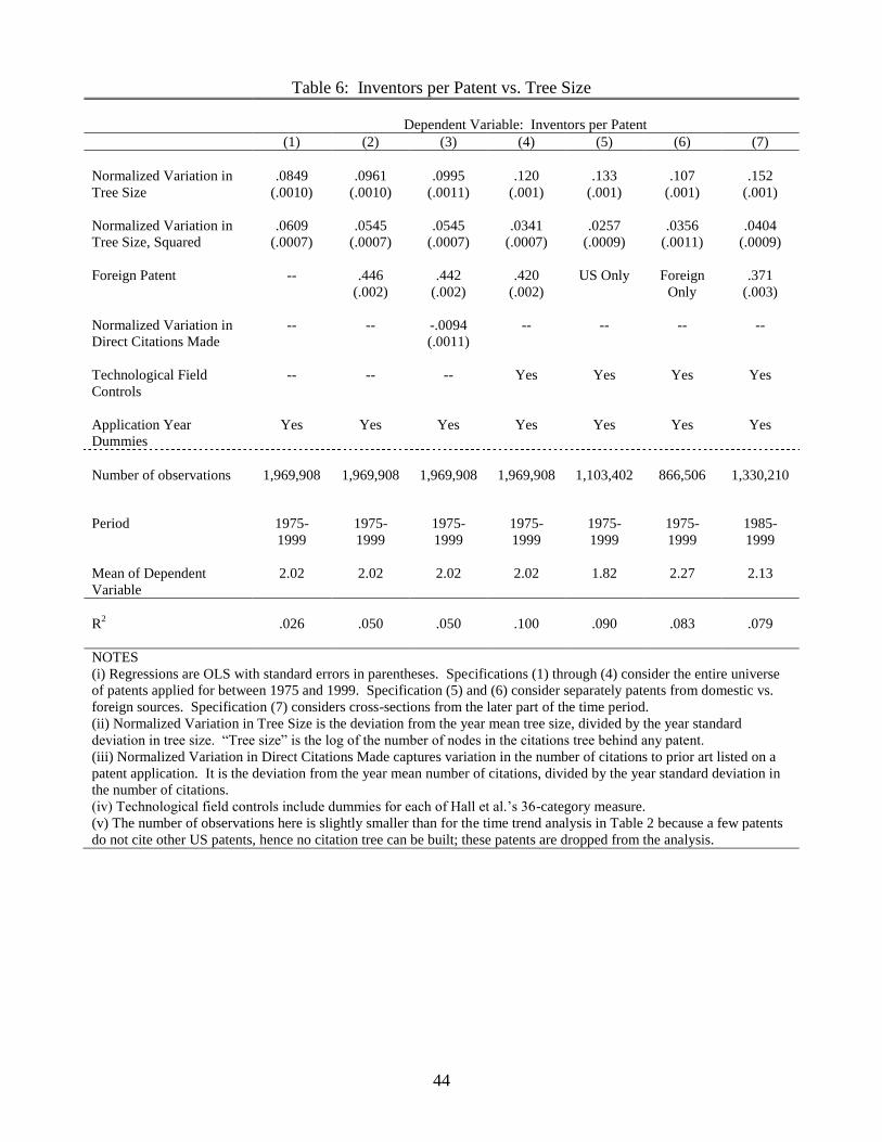
44

Table 6: Inventors per Patent vs. Tree Size

Dependent Variable: Inventors per Patent

(1)

(2)

(3) (4) (5) (6) (7)

Normalized Variation in

Tree Size

.0849

(.0010)

.0961

(.0010)

.0995

(.0011)

.120

(.001)

.133

(.001)

.107

(.001)

.152

(.001)

Normalized Variation in

Tree Size, Squared

.0609

(.0007)

.0545

(.0007)

.0545

(.0007)

.0341

(.0007)

.0257

(.0009)

.0356

(.0011)

.0404

(.0009)

Foreign Patent

--

.446

(.002)

.442

(.002)

.420

(.002)

US Only

Foreign

Only

.371

(.003)

Normalized Variation in

Direct Citations Made

-- -- -.0094

(.0011)

-- -- -- --

Technological Field

Controls

--

--

--

Yes

Yes

Yes

Yes

Application Year

Dummies

Yes Yes Yes Yes Yes Yes Yes

Number of observations

1,969,908

1,969,908

1,969,908

1,969,908

1,103,402

866,506

1,330,210

Period

1975-

1999

1975-

1999

1975-

1999

1975-

1999

1975-

1999

1975-

1999

1985-

1999

Mean of Dependent

Variable

2.02

2.02

2.02

2.02

1.82

2.27

2.13

R2

.026

.050

.050

.100

.090

.083

.079

NOTES

(i) Regressions are OLS with standard errors in parentheses. Specifications (1) through (4) consider the entire universe

of patents applied for between 1975 and 1999. Specification (5) and (6) consider separately patents from domestic vs.

foreign sources. Specification (7) considers cross-sections from the later part of the time period.

(ii) Normalized Variation in Tree Size is the deviation from the year mean tree size, divided by the year standard

deviation in tree size. ―Tree size‖ is the log of the number of nodes in the citations tree behind any patent.

(iii) Normalized Variation in Direct Citations Made captures variation in the number of citations to prior art listed on a

patent application. It is the deviation from the year mean number of citations, divided by the year standard deviation in

the number of citations.

(iv) Technological field controls include dummies for each of Hall et al.’s 36-category measure.

(v) The number of observations here is slightly smaller than for the time trend analysis in Table 2 because a few patents

do not cite other US patents, hence no citation tree can be built; these patents are dropped from the analysis.

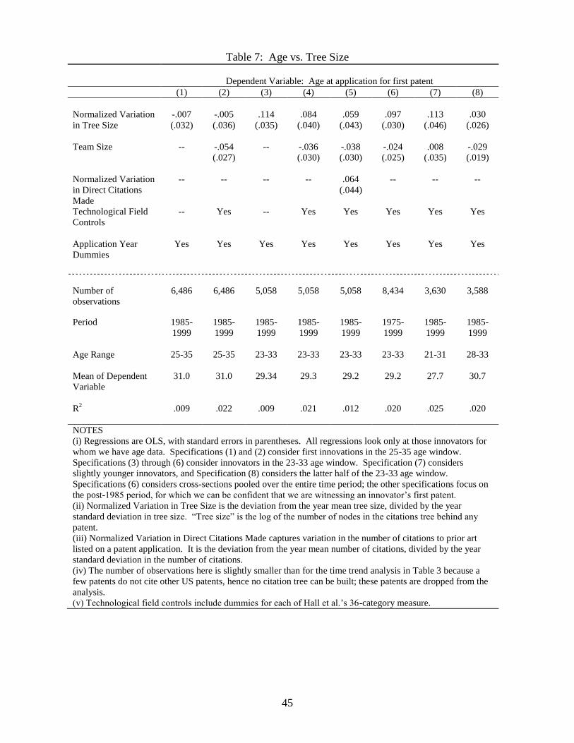
45

Table 7: Age vs. Tree Size

Dependent Variable: Age at application for first patent

(1) (2) (3) (4)

(5) (6) (7) (8)

Normalized Variation

in Tree Size

-.007

(.032)

-.005

(.036)

.114

(.035)

.084

(.040)

.059

(.043)

.097

(.030)

.113

(.046)

.030

(.026)

Team Size

-- -.054

(.027)

-- -.036

(.030)

-.038

(.030)

-.024

(.025)

.008

(.035)

-.029

(.019)

Normalized Variation

in Direct Citations

Made

-- -- -- -- .064

(.044)

-- -- --

Technological Field

Controls

-- Yes -- Yes Yes Yes Yes Yes

Application Year

Dummies

Yes Yes Yes Yes Yes Yes Yes Yes

Number of

observations

6,486

6,486

5,058

5,058

5,058

8,434

3,630

3,588

Period

1985-

1999

1985-

1999

1985-

1999

1985-

1999

1985-

1999

1975-

1999

1985-

1999

1985-

1999

Age Range 25-35 25-35 23-33 23-33 23-33 23-33 21-31 28-33

Mean of Dependent

Variable

31.0

31.0

29.34

29.3

29.2

29.2

27.7

30.7

R2

.009

.022

.009

.021

.012

.020

.025

.020

NOTES

(i) Regressions are OLS, with standard errors in parentheses. All regressions look only at those innovators for

whom we have age data. Specifications (1) and (2) consider first innovations in the 25-35 age window.

Specifications (3) through (6) consider innovators in the 23-33 age window. Specification (7) considers

slightly younger innovators, and Specification (8) considers the latter half of the 23-33 age window.

Specifications (6) considers cross-sections pooled over the entire time period; the other specifications focus on

the post-1985 period, for which we can be confident that we are witnessing an innovator’s first patent.

(ii) Normalized Variation in Tree Size is the deviation from the year mean tree size, divided by the year

standard deviation in tree size. ―Tree size‖ is the log of the number of nodes in the citations tree behind any

patent.

(iii) Normalized Variation in Direct Citations Made captures variation in the number of citations to prior art

listed on a patent application. It is the deviation from the year mean number of citations, divided by the year

standard deviation in the number of citations.

(iv) The number of observations here is slightly smaller than for the time trend analysis in Table 3 because a

few patents do not cite other US patents, hence no citation tree can be built; these patents are dropped from the

analysis.

(v) Technological field controls include dummies for each of Hall et al.’s 36-category measure.

46

Table 8: Field Jump vs. Tree Size

Dependent Variable: Probability of Switching Technological Field

(1)

(2) (3)

(4) (5) (6)

Normalized Variation

in Tree Size

-.0072

(.0008)

-.0074

(.0008)

-.0059

(.0008)

-.0095

(.0009)

-.0144

(.0012)

-.0184

(.0017)

Foreign Patent

-- -.0125

(.0018)

-.0108

(.0018)

-.0129

(.0018)

-.0135

(.0023)

.0032

(.0032)

Time Between

Applications -- -- .0226

(.0004)

.0232

(.0004)

.0215

(.0012)

.0143

(.0017)

Technological Field

Controls (first patent)

--

--

--

Yes

Yes

Yes

Application Year

Dummies

Yes

Yes

Yes

Yes

Yes

Yes

Number of observations

353,762

353,762

353,762

353,762

212,274

110,511

Period

1975-

1999

1975-

1999

1975-

1999

1975-

1999

1975-

1993

1985-

1993

Mean of Dependent

Variable

.551

.551

.551

.551

.536

.520

(Pseudo) R2

.0039

.0039

.0117

.0251

.

.0171

.0159

NOTES

(i) Results are for probit estimation, with coefficients reported at mean values and standard errors in

parentheses. The coefficient for the Foreign dummy is reported over the 0-1 range. Only solo inventors

are considered. Specifications (1) through (4) consider the entire set of solo inventors. Specification (5)

considers only those solo inventors who meet the criteria in Specifications (1) through (6) in Table 4 (to

help control for any truncation bias in the specialization measure – see the discussion of Table 4 in the

text). Specification (6) considers the same data as Specification (5), but only looks at cross-sections in

the later part of the time period.

(ii) The dependent variable is 0 if an inventor does not switch fields between two consecutive

innovations. The field is defined using the 414-category technological class definition of the USPTO.

(iii) Normalized Variation in Tree Size is the deviation from the year mean tree size, divided by the year

standard deviation in tree size. ―Tree size‖ is the log of the number of nodes in the citations tree behind

any patent.

(iv) Technological field controls include dummies for each of Hall et al.’s 36-category measure.

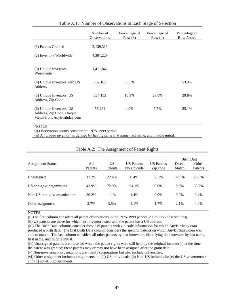
47

Table A.1: Number of Observations at Each Stage of Selection

Number of

Observations

Percentage of

Row (3)

Percentage of

Row (4)

Percentage of

Row Above

(1) Patents Granted

2,139,313

(2) Inventors Worldwide

4,301,229

(3) Unique Inventors

Worldwide

1,411,842

(4) Unique Inventors with US

Address

752,163 53.3% 53.3%

(5) Unique Inventors, US

Address, Zip Code

224,152 15.9% 29.8% 29.8%

(6) Unique Inventors, US

Address, Zip Code, Unique

Match from AnyBirthday.com

56,281 4.0% 7.5% 25.1%

NOTES

(i) Observation counts consider the 1975-1999 period.

(ii) A ―unique inventor‖ is defined by having same first name, last name, and middle initial.

Table A.2: The Assignment of Patent Rights

Birth Data

Assignment Status All

Patents

US

Patents

US Patents

No zip code

US Patents

Zip code

Direct

Match

Other

Patents

Unassigned

17.2%

22.4%

0.4%

98.3%

97.9%

26.6%

US non-govt organization

43.9% 72.9% 94.1% 0.0% 0.0% 65.7%

Non-US non-govt organization

36.2% 1.1% 1.4% 0.0% 0.0% 3.4%

Other assignment

2.7% 3.5% 4.1% 1.7% 2.1% 4.4%

NOTES

(i) The first column considers all patent observations in the 1975-1999 period (2.1 million observations).

(ii) US patents are those for which first inventor listed with the patent has a US address.

(iii) The Birth Data columns consider those US patents with zip code information for which AnyBirthday.com

produced a birth date. The first Birth Data column considers the specific patents on which AnyBirthday.com was

able to match. The last column considers all other patents by that innovator, identifying the innovator by last name,

first name, and middle initial.

(iv) Unassigned patents are those for which the patent rights were still held by the original inventor(s) at the time

the patent was granted; these patents may or may not have been assigned after the grant date.

(v) Non-government organizations are mainly corporations but also include universities.

(vi) Other assignment includes assignments to: (a) US individuals; (b) Non-US individuals; (c) the US government;

and (d) non-US governments.

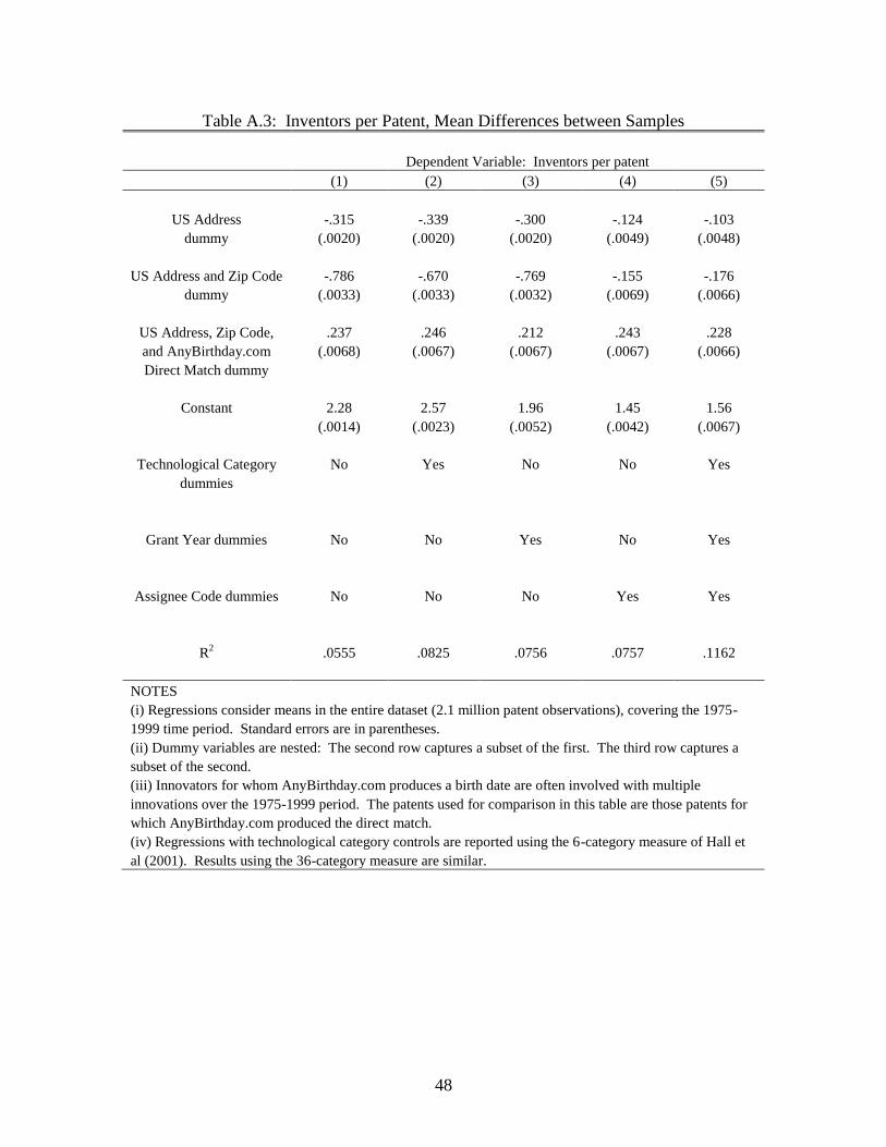
48

Table A.3: Inventors per Patent, Mean Differences between Samples

Dependent Variable: Inventors per patent

(1) (2) (3) (4) (5)

US Address

dummy

-.315

(.0020)

-.339

(.0020)

-.300

(.0020)

-.124

(.0049)

-.103

(.0048)

US Address and Zip Code

dummy

-.786

(.0033)

-.670

(.0033)

-.769

(.0032)

-.155

(.0069)

-.176

(.0066)

US Address, Zip Code,

and AnyBirthday.com

Direct Match dummy

.237

(.0068)

.246

(.0067)

.212

(.0067)

.243

(.0067)

.228

(.0066)

Constant

2.28

(.0014)

2.57

(.0023)

1.96

(.0052)

1.45

(.0042)

1.56

(.0067)

Technological Category

dummies

No

Yes

No

No

Yes

Grant Year dummies

No

No

Yes

No

Yes

Assignee Code dummies

No

No

No

Yes

Yes

R2

.0555

.0825

.0756

.0757

.1162

NOTES

(i) Regressions consider means in the entire dataset (2.1 million patent observations), covering the 1975-

1999 time period. Standard errors are in parentheses.

(ii) Dummy variables are nested: The second row captures a subset of the first. The third row captures a

subset of the second.

(iii) Innovators for whom AnyBirthday.com produces a birth date are often involved with multiple

innovations over the 1975-1999 period. The patents used for comparison in this table are those patents for

which AnyBirthday.com produced the direct match.

(iv) Regressions with technological category controls are reported using the 6-category measure of Hall et

al (2001). Results using the 36-category measure are similar.

49

30.5

30.8

31.1

31.4

31.7

1985 1987 1989 1991 1993 1995 1997 1999

Application Year

Age

Trend in Age at 'First Innovation'

.51

.53

.55

.57

Pro

ba

bili

ty o

f F

ield

Ju

mp

1975 1977 1979 1981 1983 1985 1987 1989 1991 1993Application Year

Trend in Field Jump for 'Fast' Innovators

1.6

1.7

1.8

1.9

22

.12

.22

.32

.4

1975 1979 1983 1987 1991 1995 1999Application Year

Ave

rag

e In

ven

tors

Pe

r P

ate

nt

Trends in Average Inventors Per Patent

Figure 1: Basic Time Trends