the big march: migratory flows after the ... big...the big march: migratory flows after the...

THE BIG MARCH: MIGRATORY FLOWS AFTER THE PARTITION OF INDIA

PRASHANT BHARADWAJ, ASIM KHWAJA & ATIF MIAN†

ABSTRACT. The partition of India in 1947 along religious grounds into India, Pakistan, andwhat eventually became Bangladesh, resulted in one of the largest and most rapid migrationsin human history. We compile district level census data from archives to quantify the scale ofmigratory flows across the sub-continent. We estimate total migratory inflows of 14.49 millionand outflows of 16.7 million, leading to 2.2 million "missing" people. We also uncover a sub-stantial degree of regional variability. Flows were much larger along the western border, higherin cities and areas close to the border, and dependent heavily on the size of the "minority" re-ligious group. There is almost a one for one "replacement effect" with in-moving populationsreplacing out-moving population from a district.

† YALE UNIVERSITY, HARVARD KSG & CHICAGO GSBE-mail address: [email protected]: February 2008.Thanks to Sugata Bose, Michael Boozer, Tim Guinnane, Ayesha Jalal, Saumitra Jha, T.N. Srinivasan and StevenWilkinson for comments on earlier drafts of this paper. We also thank the South Asia Initiative at Harvard forfunding part of this project. Thanks to James Nye at the University of Chicago Library for access to the IndiaOffice records. Mytili Bala and Irfan Siddiqui provided excellent research assistance.

1

2 BHARADWAJ, KHWAJA & MIAN

1. INTRODUCTION

Involuntary migrations continue to play an important role in today’s world, with warsand political strife forcing hundreds of thousands to flee. Whether it is Rwanda, Bosnia-Yugoslavia, or Israel, people are constantly faced with situations where they have no choicebut to flee. The U.S. Committee for Refugees and Immigrants estimates a total of 12 millionrefugees and an additional 21 million internally displaced people in the world (World RefugeeSurvey 2006). Yet despite the large scale and costly ramifications of these flows, our empiricalunderstanding of even the very basic questions - such as the size and variability of these flows- remains limited. How many people moved? From where and to where? How did the flowsdiffer across regions? Too many of these questions often remain unanswered

Unlike voluntary migrations - where individuals move by choice and not due to safetyconcerns - involuntary movements are harder to study because they are almost invariablydriven and accompanied by extraordinary events such as wars, partition, and ethnic/religiousstrife. They also often involve the movement of a large number of people in a very short spanof time. These events make it all the more harder to gather basic demographic information,and even in their aftermath such data are hard to recall.

The partition of India in August 1947 is one such example. Despite being one of thelargest and most rapid migrations in human history with an estimated 14.5 million peoplemigrating within four years, there is little analytic work that examines the nature or conse-quences of this rapid movement.1 However, at least in this case, the lack of quantitative datais not an issue. There is extensive and detailed data available both for the periods beforepartition (during the British period), as well as after partition. This therefore offers a uniqueopportunity for a more quantitative analysis.

A contribution of this work is to compile historical data sources in a manner that isamenable for empirical analysis and at a disaggregated enough level - the district. Doing soprovides a more detailed picture of the migratory flows and allows for comparisons acrosstime. This is a challenging task, particularly since administrative boundaries underwent sub-stantial change after partition. While this data will form the basis of a series of studies thatultimately examines the socio-economic consequences of the large flows, in this paper we willfocus on the size and nature of the flows. In a related follow-up paper (Bharadwaj, Khwajaand Mian 2007a), we examine the demographic consequences of the flows.

Using the 1931 and 1951 population census data we find that by 1951, 14.49 millionpeople had migrated into India, Pakistan, and what later became Bangladesh. While out-flows are not directly reported, we use region specific population projections to estimate totaloutflows of 16.7 million people during the same period. This suggests there were 2.2 millionpeople "missing" or unaccounted for during the partition.

1For a literature review please see Bharadwaj, Khwaja & Mian, 2007, hereon BKM

THE BIG MARCH 3

While these numbers underscore how large and sudden involuntary flows can be, theyhide substantial variation. Although both the western (between India and Pakistan) and east-ern border (between India and Bangladesh) regions had large populations, migratory flowsalong the western border were almost three times as large. The flows on the western borderwere also substantial relative to the existing population: Pakistani Punjab saw 19.7% of itspopulation leave while by 1951, 25.5% of its population was from across the border; in IndianPunjab, 40.4% of the population left and 18.8% of the population was migrants. In compar-ison, West Bengal (on the Indian side) saw only 6.7% of its population leave to be replacedby migrants who constituted only 4.7% of the population. On the Bangladeshi side, 8% ofthe population left and 3% of the population was migrant by 1951. Thus, while the partitionwas along religious lines, those along the western border were much more likely to move,presumably due to greater perceived threats.

In addition to variation between the two borders, the disaggregated results show highvariation in flows even across nearby districts both in absolute numbers and as a fraction ofthe district’s population. For example, the districts of Nadia and Murshiadabad in West Ben-gal (India) are right on the border, yet Nadia received almost 427,000 migrants while Mur-shiadabad received only around 58,700. This suggests that migratory flows can be highlylocalized and even areas in close proximity can be faced with very different numbers.

Using district level variation also allows us to ask where migrants moved to and wherethey left from. This allow us to document that even involuntary migrations have a degree ofpredictability. Not surprisingly, distance to the border plays a significant role with migrantsboth more likely to leave from and migrate to closer places. Similarly, larger cities are morelikely to be destinations for migrants. However, these are by no means the primary factors.

Given that partition was on religious grounds it is not surprising that the dominantfactor determining out-migration, especially along the western border, was religion. Indiandistricts with greater numbers of Muslims and Pakistani/Bangladeshi districts with greaternumber of Hindus and Sikhs saw greater outflows. Along the western border this religious"minority" exit is quite stark: The percentage of Muslims fell from 32 percent in 1931 to 1.8percent by 1951 in districts that were eventually in Indian Punjab. Similarly, in the districtsthat became part of Pakistani Punjab, the percentage of Hindus and Sikhs fell from 22 percentto 0.16%!

What is perhaps most surprising is that there is a large "replacement effect" in de-termining where migrants went - migrants moved almost one for one into the same ar-eas/districts that saw greater outflows. For example, Delhi had 0.45 million people movingout to be replaced by 0.5 million people from across the border (about 28% of the populationof 1951). This replacement effect is all the more remarkable given that it is over and above anydistance effect, i.e. when comparing close by districts we find that those with greater outflowsare precisely the ones with greater inflows. For example, Ajmer district, approximately samedistance from the border as Delhi, had about 72,500 people move out and 71,300 people movein (only about 10% of the population). Whether these in-migrants were allotted the property


of those leaving is a much harder question to answer given the available data, yet our re-sults do hint at this. More broadly they suggest that despite all the chaos that accompaniesinvoluntary migrations, they can display a surprising degree of predictability.

In the subsequent sections we detail the construction of the data and variables of inter-est and then present the results. The data and methodology is of particular interest, and bymaking it available to a wider group2 we hope that it can form the basis of further work thatcan start examining both the short and long term consequences of the Indian partition andmore generally of involuntary migrations.

2. DATA AND VARIABLES

The primary source of data used to compare pre and post-partition movements are the1931 census of British India and the 1951 censuses of India and Pakistan. Since there is somecontroversy regarding the quality and coverage of the 1941 census, with most demographersnot considering it to be reliable, we use the 1931 census instead to obtain pre-partition demo-graphics.3 An important issue in using the two censuses, however, is identifying comparableenumeration areas. We describe how we address this issue and the construction of primarymeasures below. British India was divided into states which in turn were subdivided into dis-tricts.4 In order to be able to present a detailed analysis, an important consideration for thisstudy was to compile data at the lowest feasible geographical unit - the district. The districtis the lowest administrative unit at which we are consistently able to find demographic data.Moreover, identifying the same geographical units over time becomes nearly impossible ifone were to try and use lower administrative units such as tehsils.

Mapping districts pre and post partition is a challenging task. Not surprisingly, theboundary creation as a result of partition was accompanied by substantial reorganization ofstate and district boundaries, not just for those regions that were split across the two countriesbut even within these countries. This was particularly true in areas where there were a lot ofprincely states since these states were by and large integrated into the provinces and districtsof the new countries. At times a district was split into two, or smaller districts merged intoone for administrative or political reasons. Thus, district names need not match up betweenthe two censuses, and even if they do there is no guarantee that they represent the same ge-ographical area. An important contribution of our work has been constructing district levelmappings between the two censuses. We do so by using detailed administrative maps from

2We hope to make all the basic census data collected available on the website hosted by the South Asia Initiativeat Harvard University.3The introduction to the 1941 census itself raises concerns about quality and coverage of the census, with thecensus commissioner admitting that "There was a tendency in the more communal quarters to look on the censusenumerators as the ready tools of faction" (pg. 9) and that "The main point [about completion of enumeration]which emerges at once is that the great population regions of the Indus and Ganges systems in which nearly halfthe total population of India lies have only a limited representation in the census figure" (pg 11). More details arein the Appendix4For more on the British spatial system, see Kant (1988)

THE BIG MARCH 5

the two census periods to identify comparable areas and then comparing census data on re-ported land areas to ensure that our visual match was accurate. In several cases, the only fea-sible comparison entailed combining (typically adjacent) districts in 1931 and/or 1951. Thematching process is described in more detail in the Appendix. Only a few districts could notbe mapped. We were able to map 462 of the 472 districts and princely states of British Indiain 1931 and 363 of the 373 districts in India and Pakistan in 1951. Since some districts had tobe merged we obtain a total of 287 comparable "districts" between the two census years.

There are two main variables used in our analysis: Inflows, the number of peoplemoving into an area due to partition, and outflows, the number of people moving out. Wedescribe how both are obtained.

2.1. Inflows. : An important variable we use in our analysis is the number of people whomigrated into a district due to partition - the inflows of migrants into the district. Thesenumbers are obtained directly from the census since both the 1951 censuses of India andPakistan explicitly asked census respondents whether they had migrated during the partition.In the Indian census the term used for such migrants was "displaced persons," while thePakistani census uses the term "muhajir." Displaced and muhajir specifically measure peoplethat moved from India/Pakistan due to partition. Internal migration is not measured by thisvariable and therefore it provides a good measure of the number of people who moved intoboth countries due to the partition. 5

2.2. Outflows. : Equally important is a measure of the number of people who left a districtdue to partition - outflows. Unfortunately, the census data provides no direct way of estimat-ing this number.6However, the fact that the migratory flows were essentially entirely alongreligious lines provides us with a methodology to estimate such outflows. While the method-ology is admittedly rough, it does provide us with a sense of the magnitude and variabilityof outflows.

The methodology we use exploits the fact that the migratory flows were almost en-tirely along religious lines. Outflows are therefore considered to be Muslims leaving India(for Pakistan/Bangladesh) and Hindus and Sikhs leaving Pakistan and Bangladesh (for In-dia). To simplify terminology we abuse notation slightly, by henceforth referring to thesegroups as "minorities." Hindus and Sikhs are minorities in Pakistan and Muslims are minori-ties in India. The remaining groups in both countries will be referred to as the " majority."Note that we do not include other religious groups such as Christians, Buddhists, etc. asminorities since these groups were not thought to have been as affected in either country.7

5These numbers could be inaccurate if individuals misreported their migrant status. However, we have littlereason to suspect that there were significant incentives to do so.6Unlike migrants into a district that can be directly ascertained by asking a person’s status in 1951, there is nosimple way to ask how many people left. The direct way would have been to ask the migrants in 1951 whichdistrict they migrated from, but to our knowledge no such information was solicited in the census.7see http://www.ishr.org/activities/religiousfreedom/pakistan-india-bangladesh.htm. Downloaded September2006.


Consistent with this assumption we find that the percentage of Christians in India and Pak-istan stayed relatively constant in 1931 and 1951. In order to compute outflows we need toestimate how many minorities left a district. The main issue in arriving at this number is toestimate the counterfactual of how many minorities would there have been in a district hadpartition not occurred. Once this counterfactual, expected minorities, is estimated, outflows canbe computed by subtracting the actual number of minorities in a district in 1951 from the ex-pected minorities estimated for that district. So the main challenge is estimating the expectedminorities in a district.

An example will illustrate. Suppose that an Indian district had 100,000 Muslims inthe 1931 census. The 1951 census shows that this district had 50,000 Muslims. Suppose theexpected growth rate for Muslims in the twenty year period between 1931 and 1951 was adoubling of the population. Given the 1931 numbers, the expected number of Muslims in1951 to have been 200,000. This gives total outflows in the district as 150,000 (i.e. 200,000 -50,000).

The accuracy of this calculation primarily relies on two assumptions. First, that flowsdue to partition from a district were indeed religion specific (i.e. Muslims were unlikely tomigrate to India). Second, that we have correctly imputed the minority growth rate. Boththe anecdotal evidence and data suggests that the first is likely to be true with the exceptionof maybe a few districts, particularly in Bengal (i.e. along the eastern border).8 However,estimating the counterfactual minority growth rate is a harder task and of particular concernas even small differences in growth rates can lead to large differences in absolute numbers.

To compute the minority growth rate from 1931 to 1951 we clearly cannot directlyuse 1951 minority numbers as these numbers changed due to the partition. Nevertheless,since the 1951 census reports majority numbers separately for residents and migrants, we cancalculate the growth rate for the majority group that is not directly affected by the partitionflows. This is not enough, however, since imposing the majority growth rate on the minoritypopulation is likely to be problematic since the minority and majority groups typically haddifferent growth rates prior to partition. To address this problem we use a "scaling factor"which is the ratio of minority to majority growth rates from the previous twenty year period,1901 to 1921. The 1931-1951 majority growth rate is then rescaled by this factor to obtainthe desired 1931-1951 minority growth rate. An alternate and apparently simpler methodwould have been to directly use the 1931-1941 (or 1901-1921) growth rate of minorities9 todetermine the 1931-1951 minority growth rates. While we construct this measure and alsopresent outflow estimates using it in the Appendix, we prefer not to use it since it makes amuch stronger assumption in the data - that population growth rates did not significantly

8Unfortunately since the census does not ask the religion of migrants there is no direct way to test this in the data.9One major reason to not use this growth rate is that the Bengal famine occurred in 1943-44 and reportedly killedabout 4 million people. Hence our estimates for expected minorities would then include people that died dueto the famine, which makes mortality estimates due to partition more difficult to calculate. By using 1931-1951growth rates of majorities, we do assume that majority and minority groups had an equal probability of dyingduring the famine.

THE BIG MARCH 7

change over time. While this is truer for states along the western border (where the twomethods in fact give similar outflow numbers), the high mortality due to the Bengal faminein 1943-44 meant that this was not true for the eastern states. We discuss these issues in moredetail in the Appendix.

3. RESULTS

3.1. Overall Flows. Inflows: The total inflows into all three countries combined, measuredin 1951, was 14.49 million or about 3.3% of the total population at the time. However, thispercentage hides substantial differences in the relative importance of flows. The absolutenumber of migrants into India was 7.3 million, into Pakistan 6.5 million, and into Bangladesharound 0.7 million. As a percentage of their populations these numbers are 2.04%, 20.9% and1.66% respectively. Migrants into Pakistan were clearly a very substantial presence.10

Outflows: While necessarily more tentative given the assumptions needed to constructthem, we estimate that there were total outflows of 16.8 million from all three countries com-bined.11 The outflow numbers for the three countries are 8.5 million out of India, about 5.4million out of Pakistan, and 2.9 million out of Bangladesh. For numbers obtained using dif-ferent methods of computing outflows, please see Appendix .

Interestingly, while outflows relative to the total population are in similar proportionsas inflows were in India and Pakistan (2.36% and 17.4% respectively) with Pakistan experi-encing relatively large outflows (and inflows), in Bangladesh outflows were much larger thaninflows both in absolute and relative terms. As a percentage of Bangladesh’s population,outflows were a sizeable 7.03% (as compared 1.6% for inflows).

Missing Persons: Since outflows represent people who left and inflows those whoeventually arrived, by subtracting total inflows from total outflows we can obtain an estimateof the total number of "missing" people. We estimate a total of 2.2 million missing due to thepartition. To the extent that the outflow measures are estimated accurately, this missing num-ber includes people who died during partition and those who migrated to another country(apart from India, Pakistan or Bangladesh). While precise numbers are not available for thelatter it is likely that it was not that significant, suggesting that, to the extent that the outflowcalculations are accurate, the greater part of the missing number is likely to reflect mortalityduring partition.

These estimates are fairly large but consistent with accounts in the literature. LawrenceJames notes that "Sir Francis Mudie, the governor of West Punjab, estimated that 500,000

10To put the number for India in perspective, we calculate from Srivastava and Sasikumar (2003) that internalmigration rate in India was around 11% in 1992. Hence an impact of 2% in migration in 1951 is a potentially largeeffect.11These numbers are estimated in terms of 1951 population levels, i.e., given our construction they also includeany children born between 1947 and 1951 for the out-migrating families. We do so because the numbers forinflows are also in 1951 and therefore include children born to the in-migrants. One could convert these numbersinto 1947 numbers by discounting the numbers by the population growth rate between 1947 and 1951. However,we prefer not to do so both because such accurate birth and mortality rate data is not available and also becausethese flows did not only occur in 1947 but continued for a few years.


Muslims died trying to enter his province, while the British High Commissioner in Karachiput the full total at 800,000. . . . This makes nonsense of the claim by Mountbatten and hispartisans that only 200,000 were killed."(1997, pg 636) Our estimate for the number of missingMuslims who left western India but did not arrive into western Pakistan is 0.66 million, closeto the number cited above by James. The corresponding missing Hindus/Sikhs along thewestern border (i.e. migrants arriving in western India) is 0.85 million. Along the easternborder, our estimates are 0.59 missing Muslims in Bangladesh (those Muslims who left Indiabut were not accounted for in arrivals into Bangladesh) and 0.24 million missing Hindus andSikhs in the eastern Indian States.

3.2. Differences in Flows across Regions. Not surprisingly, migratory flows vary signifi-cantly across states with those closer to the borders both sending and receiving greater flows.However, what is somewhat surprising is that there is a substantial variation in these flowsacross districts within the same states, suggesting that distance was not the only factor. Whilewe will try to determine the factors that influenced migration, in this section we simply illus-trate the differences in migratory flows across districts.

3.2.1. Inflows. Figure 1 shows inflows into each district in terms of absolute numbers and as apercentage of the district population. Since we will make use of such figures subsequently, itis important to explain this figure more carefully. Each point on the figure represents inflowsinto a particular district. The X-axis of this graph labels the state these districts belong to(thus all districts in a given state are plotted along the same vertical line). States are roughlyorganized from west to east within each country so the graph is akin to converting a map ofthe region into a single line "map." 12 The western and eastern borders are plotted as verticallines for reference. Note that the distance between states in the figure does not reflect actualdistance between them. We will provide graphs that show actual distance later.

The graphs illustrate several patterns. First, the migratory inflows that took place inthe aftermath of partition were primarily centered around Punjab (Indian and Pakistani), WestBengal, and Bangladesh. The separation of over 2000 km between Punjab and Bengal there-fore made for 2 centers of partition in India with other states in playing a minor role in receiv-ing displaced persons.

Second, the western and eastern borders experienced different dynamics of partition.Till 1951 the flows on the western border were almost 3 times the size of the flows on theeastern border. The west in general received about 10.7 million people while the east receivedabout 3.2 million. Moreover, while there was greater movement out of India than into italong the western border (Pakistani Punjab received about twice the number of migrantsas compared to Indian Punjab), it was the opposite along the eastern border - West Bengalreceived about twice the number of migrants as compared to Bangladesh.

12The west to east sequence is not always preserved. For example, Assam is to the east of East Bengal but sincethe former is in India and the latter in Bangladesh we distort this single-line "map" slightly in order to keep allstates in a country together, by putting Assam before East Bengal.

THE BIG MARCH 9

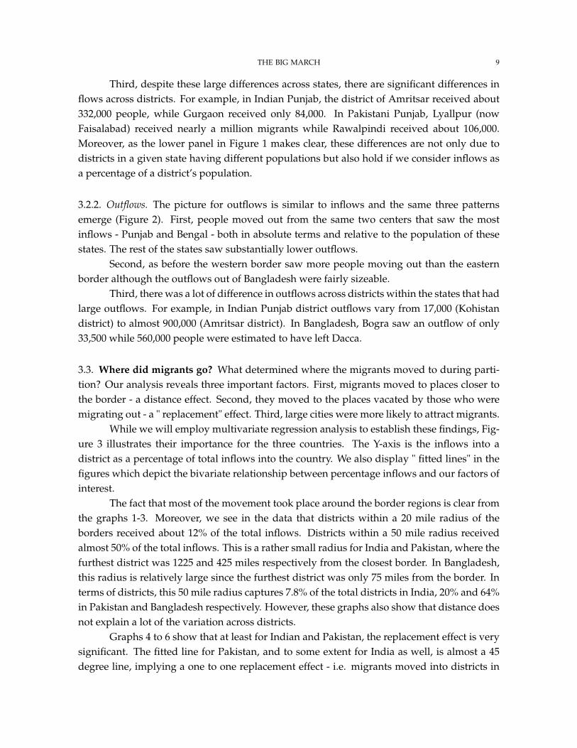
Third, despite these large differences across states, there are significant differences inflows across districts. For example, in Indian Punjab, the district of Amritsar received about332,000 people, while Gurgaon received only 84,000. In Pakistani Punjab, Lyallpur (nowFaisalabad) received nearly a million migrants while Rawalpindi received about 106,000.Moreover, as the lower panel in Figure 1 makes clear, these differences are not only due todistricts in a given state having different populations but also hold if we consider inflows asa percentage of a district’s population.

3.2.2. Outflows. The picture for outflows is similar to inflows and the same three patternsemerge (Figure 2). First, people moved out from the same two centers that saw the mostinflows - Punjab and Bengal - both in absolute terms and relative to the population of thesestates. The rest of the states saw substantially lower outflows.

Second, as before the western border saw more people moving out than the easternborder although the outflows out of Bangladesh were fairly sizeable.

Third, there was a lot of difference in outflows across districts within the states that hadlarge outflows. For example, in Indian Punjab district outflows vary from 17,000 (Kohistandistrict) to almost 900,000 (Amritsar district). In Bangladesh, Bogra saw an outflow of only33,500 while 560,000 people were estimated to have left Dacca.

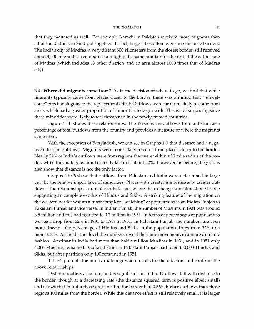
3.3. Where did migrants go? What determined where the migrants moved to during parti-tion? Our analysis reveals three important factors. First, migrants moved to places closer tothe border - a distance effect. Second, they moved to the places vacated by those who weremigrating out - a " replacement" effect. Third, large cities were more likely to attract migrants.

While we will employ multivariate regression analysis to establish these findings, Fig-ure 3 illustrates their importance for the three countries. The Y-axis is the inflows into adistrict as a percentage of total inflows into the country. We also display " fitted lines" in thefigures which depict the bivariate relationship between percentage inflows and our factors ofinterest.

The fact that most of the movement took place around the border regions is clear fromthe graphs 1-3. Moreover, we see in the data that districts within a 20 mile radius of theborders received about 12% of the total inflows. Districts within a 50 mile radius receivedalmost 50% of the total inflows. This is a rather small radius for India and Pakistan, where thefurthest district was 1225 and 425 miles respectively from the closest border. In Bangladesh,this radius is relatively large since the furthest district was only 75 miles from the border. Interms of districts, this 50 mile radius captures 7.8% of the total districts in India, 20% and 64%in Pakistan and Bangladesh respectively. However, these graphs also show that distance doesnot explain a lot of the variation across districts.

Graphs 4 to 6 show that at least for Indian and Pakistan, the replacement effect is verysignificant. The fitted line for Pakistan, and to some extent for India as well, is almost a 45degree line, implying a one to one replacement effect - i.e. migrants moved into districts in


almost perfect proportion with out-migration in these districts. This close relationship be-tween people moving out and moving in is suggestive of reallocation of evacuee property tothose migrating in. Interestingly, in Bangladesh this replacement effect is less important. AsKudaisya and Tan (2000) note, " while in Punjab the Indian government had facilitated an ’ex-change of population’, in Bengal it wanted to prevent precisely such an exchange, and took anumber of initiatives to this end." Table 1 examines these effects in multivariate regressions.The dependent variable is the same as that on the Y-axis in Figure 2, inflows as a percentageof total inflows in the country. We run separate regressions for the three countries. All regres-sions also include the district’s population as a percentage of country population to take intoaccount whether migrants may simply have moved to larger districts. We also include a " bigcity" 13 dummy variable which captures whether the district included a large city in 1931. Inaddition we also include state level fixed effects to ensure our results are not just driven bycomparing different states. Note when we include state fixed effects it is probable that mostof the distance effects are unlikely to matter as much since distance does not vary as muchacross districts within a state. So our primary interest in looking at the regressions with statefixed effects is how robust are the results for the variables which in fact do vary within a state,like outflows from a district.

Intuitively, distance would have a mostly negative effect on where people move; how-ever, this result is only statistically significant in India and generally of small size. Inflows fallwith distance to the border though at a decreasing rate (the distance squared term is positivealbeit small) and shows that for the first 100 miles inflows drop by around 0.23%. However,beyond 600 miles from the border (the maximum distance in our data is 940 miles) the addi-tional effect of distance is slightly higher inflows.

In contrast, the replacement effect is very large and holds for all three countries thoughit holds with less statistical significance in Bangladesh. Pakistan shows this replacement effectto be very important since the regression coefficient is close to one, suggesting a one-to-onemapping between those moving out and those moving in - i.e., for every one person leavingin a district they are replaced by (slightly more than) one person entering the district. It alsomatters in India, but not as closely. Since these regressions include the district’s relative popu-lation and state fixed effects, we can be assured that the replacement effect is indeed capturingreplacement and not simply that larger districts saw more in-migration or that certain stateswere more important. In fact, the insignificant coefficient on district population suggests thatthis was not an important factor at all.

Finally the results show that large cities attract more migrants. The effect holds stronglyfor India - having a large city in a district leading to 0.5% more migrants. This variable is notstatistically significant for Pakistan and Bangladesh. Part of the problem, however, is thatthere were very few big cities in these two countries (for example, Dhaka was the only ’big-city’ in our dataset for Bangladesh). Examining large cities in these countries does suggest

13Large cities are the 24 largest cities (in terms of population) from 1931. This data was obtained from the HistoricalAtlas of South Asia (Schwartzberg, 1978)

THE BIG MARCH 11

that they mattered as well. For example Karachi in Pakistan received more migrants thanall of the districts in Sind put together. In fact, large cities often overcame distance barriers.The Indian city of Madras, a very distant 800 kilometers from the closest border, still receivedabout 4,000 migrants as compared to roughly the same number for the rest of the entire stateof Madras (which includes 13 other districts and an area almost 1000 times that of Madrascity).

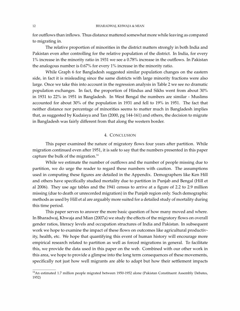
3.4. Where did migrants come from? As in the decision of where to go, we find that whilemigrants typically came from places closer to the border, there was an important " unwel-come" effect analogous to the replacement effect: Outflows were far more likely to come fromareas which had a greater proportion of minorities to begin with. This is not surprising sincethese minorities were likely to feel threatened in the newly created countries.

Figure 4 illustrates these relationships. The Y-axis is the outflows from a district as apercentage of total outflows from the country and provides a measure of where the migrantscame from.

With the exception of Bangladesh, we can see in Graphs 1-3 that distance had a nega-tive effect on outflows. Migrants were more likely to come from places closer to the border.Nearly 34% of India’s outflows were from regions that were within a 20 mile radius of the bor-der, while the analogous number for Pakistan is about 22%. However, as before, the graphsalso show that distance is not the only factor.

Graphs 4 to 6 show that outflows from Pakistan and India were determined in largepart by the relative importance of minorities. Places with greater minorities saw greater out-flows. The relationship is dramatic in Pakistan ,where the exchange was almost one to onesuggesting an complete exodus of Hindus and Sikhs. A striking feature of the migration onthe western border was an almost complete "switching" of populations from Indian Punjab toPakistani Punjab and vice versa. In Indian Punjab, the number of Muslims in 1931 was around3.5 million and this had reduced to 0.2 million in 1951. In terms of percentages of populationswe see a drop from 32% in 1931 to 1.8% in 1951. In Pakistani Punjab, the numbers are evenmore drastic - the percentage of Hindus and Sikhs in the population drops from 22% to amere 0.16%. At the district level the numbers reveal the same movement, in a more dramaticfashion. Amritsar in India had more than half a million Muslims in 1931, and in 1951 only4,000 Muslims remained. Gujrat district in Pakistani Punjab had over 130,000 Hindus andSikhs, but after partition only 100 remained in 1951.

Table 2 presents the multivariate regression results for these factors and confirms theabove relationships.

Distance matters as before, and is significant for India. Outflows fall with distance tothe border, though at a decreasing rate (the distance squared term is positive albeit small)and shows that in India those areas next to the border had 0.36% higher outflows than thoseregions 100 miles from the border. While this distance effect is still relatively small, it is larger


for outflows than inflows. Thus distance mattered somewhat more while leaving as comparedto migrating in.

The relative proportion of minorities in the district matters strongly in both India andPakistan even after controlling for the relative population of the district. In India, for every1% increase in the minority ratio in 1931 we see a 0.78% increase in the outflows. In Pakistanthe analogous number is 0.67% for every 1% increase in the minority ratio.

While Graph 6 for Bangladesh suggested similar population changes on the easternside, in fact it is misleading since the same districts with large minority fractions were alsolarge. Once we take this into account in the regression analysis in Table 2 we see no dramaticpopulation exchanges. In fact, the proportion of Hindus and Sikhs went from about 30%in 1931 to 22% in 1951 in Bangladesh. In West Bengal the numbers are similar - Muslimsaccounted for about 30% of the population in 1931 and fell to 19% in 1951. The fact thatneither distance nor percentage of minorities seems to matter much in Bangladesh impliesthat, as suggested by Kudaisya and Tan (2000, pg 144-161) and others, the decision to migratein Bangladesh was fairly different from that along the western border.

4. CONCLUSION

This paper examined the nature of migratory flows four years after partition. Whilemigration continued even after 1951, it is safe to say that the numbers presented in this papercapture the bulk of the migration.14

While we estimate the number of outflows and the number of people missing due topartition, we do urge the reader to regard these numbers with caution. The assumptionsused in computing these figures are detailed in the Appendix. Demographers like Ken Hilland others have specifically studied mortality due to partition in Punjab and Bengal (Hill etal 2006). They use age tables and the 1941 census to arrive at a figure of 2.2 to 2.9 millionmissing (due to death or unrecorded migration) in the Punjab region only. Such demographicmethods as used by Hill et al are arguably more suited for a detailed study of mortality duringthis time period.

This paper serves to answer the more basic question of how many moved and where.In Bharadwaj, Khwaja and Mian (2007a) we study the effects of the migratory flows on overallgender ratios, literacy levels and occupation structures of India and Pakistan. In subsequentwork we hope to examine the impact of these flows on outcomes like agricultural productiv-ity, health, etc. We hope that quantifying this event of human history will encourage moreempirical research related to partition as well as forced migrations in general. To facilitatethis, we provide the data used in this paper on the web. Combined with our other work inthis area, we hope to provide a glimpse into the long term consequences of these movements,specifically not just how well migrants are able to adapt but how their settlement impacts

14An estimated 1.7 million people migrated between 1950-1952 alone (Pakistan Constituent Assembly Debates,1952)

THE BIG MARCH 13

the trajectory of the places they moved to. Given the current events and importance of SouthAsia, we hope that such a historical empirical analysis may prove to be of value.


5. REFERENCES

Bharadwaj, P., Khwaja, A., Mian, A. The Partition of India: Demographic Consequences.Working Paper (2007a).

Davis, K. The Population of India and Pakistan, Princeton: Princeton University Press(1951).

Government of India, Census of India 1931, India: Central publication branch (1933).Government of India, Census of India 1941, Delhi: The Manager of Publications, (1941-

1945).Government of India, Census of India 1951, Delhi: The Manager of Publications, (1952).Government of Pakistan, Census of Pakistan 1951, Karachi: The Manager of Publica-

tions, (1954-56).Hill, K et al. The partition of India: new demographic estimates of associated population

change International Union for the Scientific Study of Population, International PopulationConference, France, 2005.

Hill, K et al. The Demographic Impact of Partition: The Punjab in 1947 Working Paper06-08, Weatherhead Center for International Affairs, Harvard University, 2006.

James, L. Raj: the making and unmaking of British India, New York: St. Martin’s Press(1998).

Kudaisya, G & Yong Tan, T. The Aftermath of Partition in South Asia, London: Routledge(2000)

Sherwani, L A. The partition of India and Mountbatten, Karachi, Council for PakistanStudies (1986).

Srivastava, R & Sasikiran SK. An Overview of Migration in India, its Impacts and KeyIssues, www.livelihoods.org.

U.S. Committee for Refugees and Immigrants. World Refugee Survey, http://www.refugees.org,2006.

THE BIG MARCH 15

6. APPENDIX

6.1. The Census of 1941. As we noted in the main text, our decision not to use the 1941census of India is based on various significant concerns regarding the quality and coverageof this census.

This is perhaps best illustrated by a series of statements by the Census Commissionerof the 1941 census, MWM Yeats, in his introductory remarks to the 1941 Census.

Yeats starts off by noting that "The war has laid its hand on the Indian census as onevery other activity of the India Government and people.. . . It was considered however thatfinancial conditions did not permit the completion of the tables and as I write this brief intro-duction I am no longer, and have not been for a year, a whole-time Census Commissioner."(pg 2) and goes on to lament that "One of the last things to be desired in a census is uncer-tainty; yet that pursued us to the end. It was till February 1940 that the Government of Indiadecided to have a census at all. A still greater difficulty was caused by the delay in decidinghow far to go with the tabulation." (pg. 2)

In addition, Yeats talks about lack of tabulation facilities, buildings and officers. Hetalks about problems with some provincial tables that had to remain unresolved becauseprovincial census officers were removed from their jobs as soon as the tables went to press,and hence were not available for further clarifications. He states that, "The main point [aboutcompletion of enumeration] which emerges at once is that the great population regions of theIndus and Ganges systems in which nearly half the total population of India lies have only alimited representation in the census figures" (pg 11) and also points out his concern regardingbiased estimates and mismeasurements since "There was a tendency in the more communalquarters to look on the census enumerators as the ready tools of faction . . . " (pg 9) and "Atthat time Mr. Gandhi’s civil disobedience campaign was in full swing and all over NorthIndia the census, as a governmental activity, incurred hostility." (pg 24)

The 1951 Pakistan census also starts (pg 1) by noting that the 1941 census "had notbeen tabulated in full owing to the war, and their accuracy has been prejudiced by the effortsof different communities to inflate their figures for political purposes"

6.2. State names on Figures. X-axis State Names Key -Pakistan: 1=Baluchistan, 2=NWFP, 3=Sind, 4=Punjab5=Western BorderIndia: 6=Punjab,7=Pepsu, 8=Himachal Pradesh, 9=Saurashtra, 10=Kutch, 11=Ajmer, 12=Ra-jasthan, 13=Delhi, 14=Bombay, 15=Uttar Pradesh, 16=Madhya Pradesh, 17=Bhopal, 18=Mad-hya Bharat, 19=Vindhya Pradesh, 20=Hyderabad, 21=Andhra, 22=Madras, 23=Mysore, 24=Tra-vancore Cochin, 25=Coorg, 26=Orissa, 27=Bihar, 28=Assam, 29=Manipur, 30=Tripura, 31=WestBengal32=Eastern BorderBangladesh: 33=East Bengal


6.3. District Mapping Over Time. Unlike later censuses, the 1951 census does not provide acomprehensive mapping of the districts in 1951 to those in previous census years. As such,our approach is to use detailed maps in 1951 and 1931 and start by visually identifying map-pings between districts in the two time periods. Once the visual exercise reveals potentialmatches between the two census years, we use census data for land areas of these regionsand only consider a mapping to be permissible if the land areas of the two units are within 10percent of each other. We also perform robustness tests with lower thresholds. If two areas donot meet these criteria we attempt to map them at higher levels of aggregation (for example,by combining adjacent districts). In the majority of cases we are able to map regions over timeand only a few districts could not be mapped. Thus for the 472 districts and Princely statesof British India in 1931 we are able to map 462. The equivalent number for the 1951 districtsis 373 mapped out of a total of 363. Since some districts had to be merged this gives us a totalof 287 comparable "districts" between the two census years.

6.4. Districts not in dataset. These districts are not in our data set because of lack of infor-mation in a certain year or merging issues.

NWFP Frontier Areas (only British areas were censused in 1931)

• Chitral• Malakand• Swat• Dir• North & South Waziristan• Khurran• Khyber

Baluchistan (one area was not censused in 1951)

• Dera Ghazi Khan

Gilgit Agency (not censused)

• Yasin• Kuh Ghizar• Punial• Tangir & Darel• Ishkuman• Gilgit• Chilas• Astor• Hunza & Nagir

Assam Hill/Tribal Areas (not censused in 1951)

• Sadiya Frontier Tract• Khasi and Jaintia Hills

THE BIG MARCH 17

Jammu and Kashmir (not censused in 1951)

• Baramula• Anantnag• Riasi• Udhampur• Chamba• Kathua• Jammu• Punch• Mirpur• Muzaffarabad

Andaman and Nicobar Islands (have missing information in the 1931 census). Sikkim (Itsstatus was uncertain in 1951 and was only inducted into state of India in 1975).

6.5. Computing Outflows.

6.5.1. Outflows - the main measure. Our method of computing outflows determines expectedminority growth rates by re-scaling the growth rates of the majority population during therelevant period (1931-1951). Note that "minorities" in Pakistan are Non-Muslims, while mi-norities in India are Muslims. "Majority" in India are Non-Muslims, while majority in Pak-istan are Muslims. We define the Resident Majority Growth Rate as:

Mg = M1951r

M1931r

Where Mr denotes resident majority. The resident majority population in 1951 is calculatedas the total population of the majority group in 1951 less the population of incoming migrants(incoming migrants belonged to the majority). Majority is defined as the population minusminority populations. In our notation, upper case M always refers to the majority, whilelower case m refers to minorities.

Next we construct the scaling factor to adjust the majority growth rate to reflect mi-nority growth rate from 1931-1951. We need a scale because, as is clear in the table below,Muslims tended to grow faster than Non-Muslims in British India.


Where Gm and GM refer to minority and majority growth rates between the relevantperiod.

We use a 20-year scale because our majority growth rate is measured over 20 years aswell. It is obvious that we cannot use 1931-1951 growth rates of minorities as a scale, sinceminorities were on the move by 1951. We need to look to previous years for a scale. We didnot use the 1941 census because its quality is suspect. Our next choice was using 1911-1931growth rates to compute the scale. However, these growth rates are likely to be very differentfrom those in 1931-51 due to large internal migrations that took place in the 1920’s. Thesemigrations were primarily located in the East, with people moving from Bengal into Assam towork on the tea estates (Davis, 1951). In comparison we are aware of no significant criticismof 1901-1921 censuses as far as religious enumeration is concerned. To avoid problems ofcountering massive internal migrations and census accuracies, we therefore use the 1901-1921growth rates to compute our scale.

Now we can impute the minority growth rate between 1931 and 1951 as:

G1931−1951m = G1931−1951

M × S

Finally we can compute the expected number of minorities in 1951.

ˆm1951 = m1931 ×G1931−1951m

Outflows is the number of expected minorities less the actual number of minorities ina given district:

Outflow = ˆm1951 −m1951

The above analysis is computed at the district level with one exception. We do nothave 1901 census figures at the district level. Hence, we just use the country wide scale on the1931-51 majority growth rate at the district level.

6.5.2. Secondary measure of outflows. The departure in this method of computing outflows isin the way we compute minority growth rates:

˜G1921−1931m = m1931

r

m1921r

In other words, rather than re-scaling the 1931-1951 majority growth rates we insteaduse the minority growth rate from 1921-1931.

Therefore, the counterfactual number of minorities in 1951 is:

˜m1951 = m1931 × ˜G1921−1931m

Outflow = ˜m1951 −m1951

The problem with this measure is that the Bengal famine occurred in 1943-44 and itseffect is hard to separate at the country level - i.e. we do not have information on how manyMuslims or Hindus died as a result of it. Hence, once we compute expected minorities in 1951,we need to subtract the deaths due to famine to get at the number missing due to partition.Given that this measure would be heavily dependent on estimates of numbers of people thatdied due to the famine, it is likely to be less accurate than the first method.

There are additional problems in using this measure along the eastern border. Bengalsaw large out migration of people moving into Assam until the 1930’s. As a result, 1921-31

THE BIG MARCH 19

growth rates are in fact lower than the actual growth rates in 1931-51 (when there was nolonger this migration into Assam) and this in turn would lead to underestimates of outflowsfrom Bangladesh. In fact, for exactly the same reason we would predict that estimates ofoutflows from the eastern part of India would be overestimated if we use the 1921-31 growthrates of non-natives (Muslims) in India. Examining these estimates shows that this is indeedthe case.

This method also suffers from the fact that growth rates of religious populations arefar from stable over decades. A glance at Table A above confirms this.

Comparing aggregates we find that while the results for India and Pakistan are aboutthe same, Bangladesh’s outflows is severely underestimated using the second measure.

For reasons stated above we believe that outflow 1 captures the out migration moreaccurately. We can also compare outflows obtained at the district level using these two meth-ods. We will see that they are essentially the same, except for the eastern region estimates.Most points are on or near the 45 degree line. The outliers are, not surprisingly are districts inAssam and Bengal, where we suspected problems with over and under estimations of growthrates.

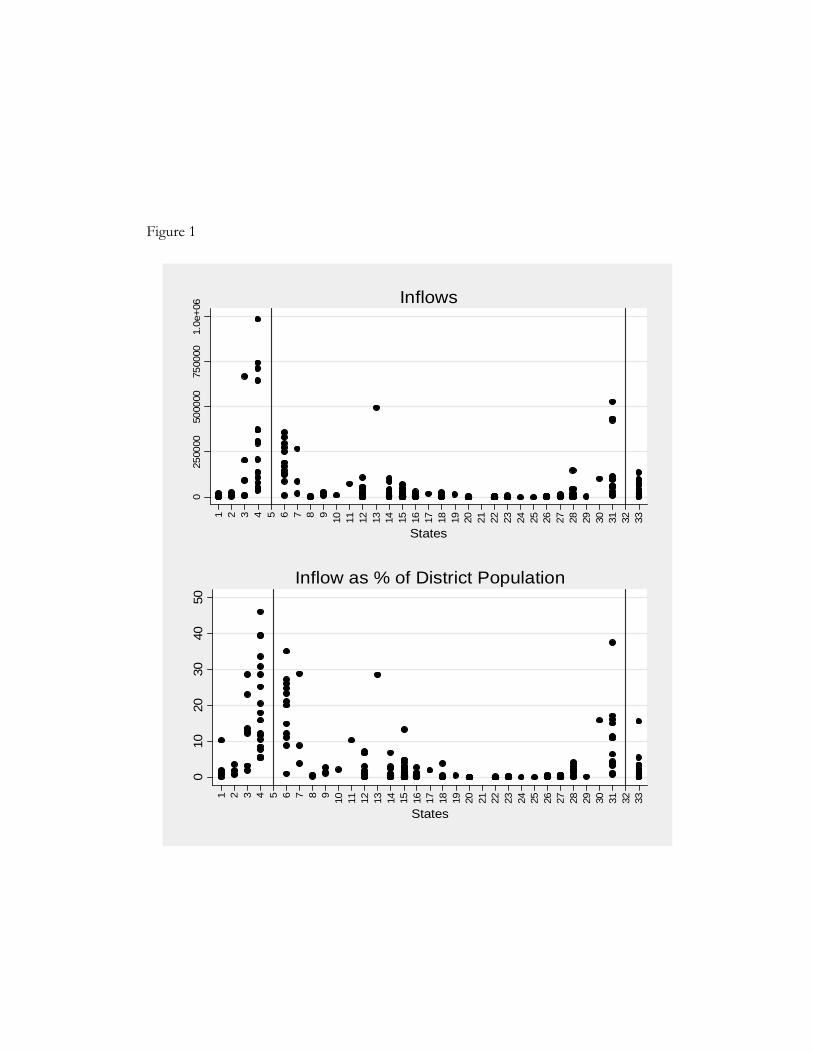
Figure 1

025

0000

5000

0075

0000

1.0e

+06

1 2 3 4 5 6 7 8 9 10 11 12 13 14 15 16 17 18 19 20 21 22 23 24 25 26 27 28 29 30 31 32 33

States

Inflows

010

2030

4050

1 2 3 4 5 6 7 8 9 10 11 12 13 14 15 16 17 18 19 20 21 22 23 24 25 26 27 28 29 30 31 32 33

States

Inflow as % of District Population

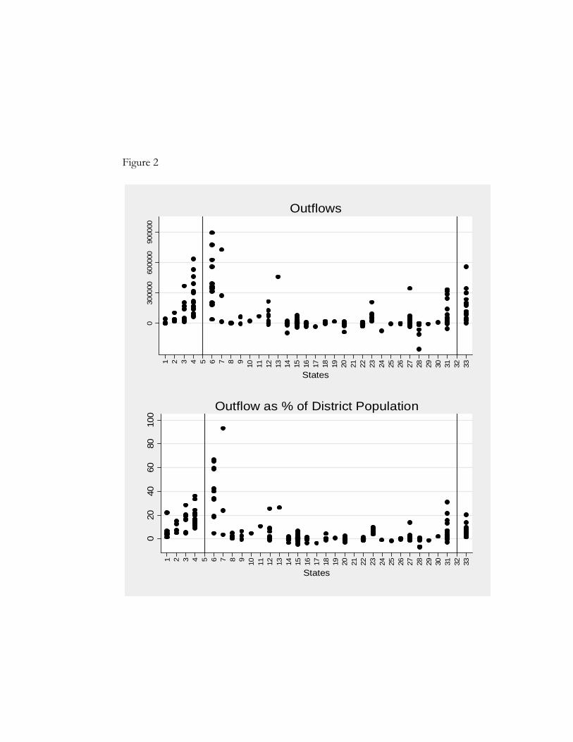
Figure 20

3000

0060

0000

9000

00

1 2 3 4 5 6 7 8 9 10 11 12 13 14 15 16 17 18 19 20 21 22 23 24 25 26 27 28 29 30 31 32 33

States

Outflows

020

4060

8010

0

1 2 3 4 5 6 7 8 9 10 11 12 13 14 15 16 17 18 19 20 21 22 23 24 25 26 27 28 29 30 31 32 33

States

Outflow as % of District Population

Figure 3

05

1015

20

2 3 4 5 6 7Log Distance from Border

1India

05

1015

20


2Pakistan

05

1015


3Bangladesh

05

1015

20

0 5 10 15 20Outflow as % of Total

4

05

1015

20


5

05

1015

20


6

Y axis is Inflows as % of Total Inflows

Where did migrants go?

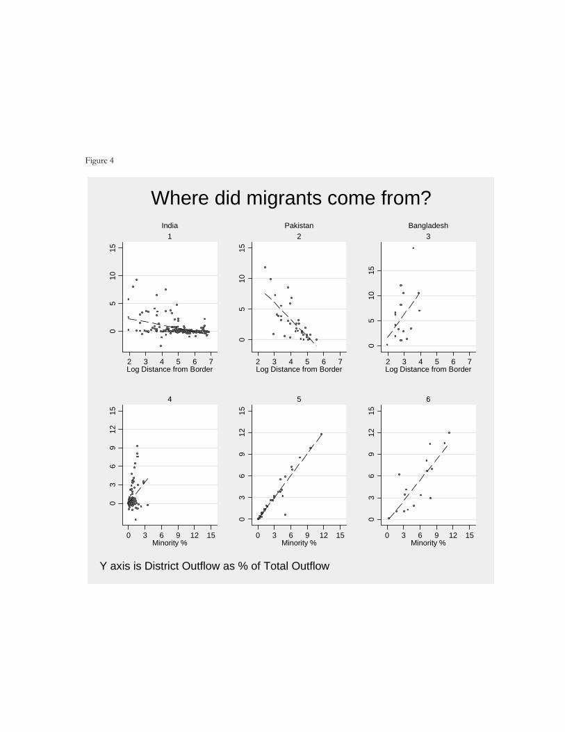
Figure 4

05

1015


1India

05

1015


2Pakistan

05

1015


3Bangladesh

03

69

1215

0 3 6 9 12 15Minority %

4

03

69

1215

0 3 6 9 12 15Minority %

5

03

69

1215

0 3 6 9 12 15Minority %

6

Y axis is District Outflow as % of Total Outflow

Where did migrants come from?

Dependent Variable: Inflows in district as % of total inflows in country(1) (2) (3) (4) (5)

BangladeshDistance (in 1000 miles) -2.522 0.012 9.003 22.011 262.624

[0.731]*** [1.161] [22.581] [31.749] [724.296]Distance Squared (/1000000) 2.133 -0.158 -21.847 -62.016 -7636.558

[0.846]** [1.114] [90.307] [106.091] [11613.805]0.539 0.535 1.145 1.169 0.954

[0.036]*** [0.049]*** [0.290]*** [0.351]*** [0.507]*City dummy 0.496 0.191 0.112 -0.501 -1.001

[0.167]*** [0.153] [1.691] [2.019] [5.495]0.06 0.155 0.221 0.38 -0.87

[0.129] [0.131] [0.470] [0.543] [0.725]Constant 0.539 0.546 -1.54 -3.57 4.59

[0.128]*** [0.603] [1.479] [2.879] [7.904]State Fixed Effects No Yes No Yes NAObservations 233 233 35 35 17R-squared 0.63 0.76 0.81 0.81 0.33Std Errors in brackets. * significant at 10%; ** significant at 5%, ***significant at 1%

This table examines the impact of distance from border, % outflow from a given district and the existence of a large city in the district on the inflows into that district. Columns 2 & 4 include state fixed effects for India and Pakistan. Bangladesh does not have state fixed effects since it has only 1 state. Computation of outflow is discussed in the Appendix. Inflows are people moving into a given district due to partition, outflows are those moving out. Distance is measured as the straight line to the nearest India-Pakistan border from the center of a district. City dummy was created from the 24 largest cities (in terms of population) from 1931. This data was obtained from the Historical Atlas of South Asia (Schwartzberg, 1978). There are 25 states in India and 4 states in Pakistan.

TABLE I

WHERE DID INCOMING MIGRANTS GO?

India Pakistan

District population as % total population in country

Outflows as % of total outflows in country

Dependent Variable: Outflows in district as % of total inflows in country(1) (2) (3) (4) (5)

BangladeshDistance (in 1000 miles) -5.034 -5.083 -3.364 -18.023 -151.274

[1.227]*** [1.519]*** [10.605] [11.845] [398.155]Distance Squared (/1000000) 5.084 3.977 28.694 55.191 3126.296

[1.413]*** [1.472]*** [40.275] [39.550] [6326.028]1.192 0.785 0.764 0.675 0.758

[0.191]*** [0.144]*** [0.130]*** [0.123]*** [0.504]City dummy 0.639 0.5 0.091 0.846 3.492

[0.280]** [0.202]** [0.746] [0.752] [2.865]-0.915 -0.383 0.558 0.486 0.445

[0.257]*** [0.205]* [0.174]*** [0.183]** [0.490]Constant 0.977 1.208 -0.833 0.742 -0.299

[0.215]*** [0.805] [0.721] [1.110] [4.295]State Fixed Effects No Yes No Yes NoObservations 233 233 35 35 17R-squared 0.31 0.72 0.94 0.95 0.73

TABLE II

WHERE DID INCOMING MIGRANTS COME FROM?

Std Errors in brackets. * significant at 10%; ** significant at 5%, ***significant at 1%

This table examines the impact of distance from border, % minorities in a given district, population size of the district and the existence of a large city in the district on the outflows from that district. Columns 2 & 4 include state fixed effects for India and Pakistan. Bangladesh does not have state fixed effects since it has only 1 state. Computation of outflow is discussed in the Appendix. Outflows are those moving out of a district due to partition. Distance is measured as the straight line to the border from the center of a district. Minorities in India are Muslims. In Pakistan and Bangladesh minorities are Hindus and Sikhs. City dummy was created from the 24 largest cities (in terms of population) from 1931. This data was obtained from the Historical Atlas of South Asia (Schwartzberg, 1978). There are 25 states in India and 4 states in Pakistan.

India Pakistan

Minorities in district as % of total minorities in country

District population as % total population in country

the big march: migratory flows after the ... big...the big march: migratory flows after the...

Documents