the bernstein polynomial basis: a centennial...
TRANSCRIPT
The Bernstein polynomial basis:
a centennial retrospective
Rida T. FaroukiDepartment of Mechanical and Aerospace Engineering,
University of California, Davis, CA 95616.
March 3, 2012
Abstract
One hundred years after the introduction of the Bernstein polynomialbasis, we survey the historical development and current state of theory,algorithms, and applications associated with this remarkable methodof representing polynomials over finite domains. Originally introducedby Sergei Natanovich Bernstein to facilitate a constructive proof of theWeierstrass approximation theorem, the leisurely convergence rate ofBernstein polynomial approximations to continuous functions causedthem to languish in obscurity, pending the advent of digital computers.With the desire to exploit the power of computers for geometric designapplications, however, the Bernstein form began to enjoy widespreaduse as a versatile means of intuitively constructing and manipulatinggeometric shapes, spurring further development of basic theory, simpleand efficient recursive algorithms, recognition of its excellent numericalstability properties, and an increasing diversification of its repertoireof applications. This survey provides a brief historical perspective onthe evolution of the Bernstein polynomial basis, and a synopsis of thecurrent state of associated algorithms and applications.
keywords: Bernstein basis; Weierstrass theorem; polynomial approximation;Bezier curves and surfaces; numerical stability; polynomial algorithms.
e–mail: [email protected]

Contents
1 Introduction 1
2 Sergei Natanovich Bernstein 2
3 Weierstrass approximation theorem 6
3.1 Existence arguments . . . . . . . . . . . . . . . . . . . . . . . 63.2 Bernstein’s constructive proof . . . . . . . . . . . . . . . . . . 73.3 Properties of the approximant . . . . . . . . . . . . . . . . . . 10
4 De Casteljau and Bezier 11
4.1 A new application emerges . . . . . . . . . . . . . . . . . . . . 124.2 Paul de Faget de Casteljau . . . . . . . . . . . . . . . . . . . . 124.3 Pierre Etienne Bezier . . . . . . . . . . . . . . . . . . . . . . . 15
5 Bernstein basis properties 18
5.1 Basic properties and algorithms . . . . . . . . . . . . . . . . . 185.2 Shape features of Bezier curves . . . . . . . . . . . . . . . . . 24
6 Numerical stability 26
6.1 Condition numbers . . . . . . . . . . . . . . . . . . . . . . . . 276.2 Wilkinson polynomial . . . . . . . . . . . . . . . . . . . . . . . 326.3 Optimal stability . . . . . . . . . . . . . . . . . . . . . . . . . 336.4 The Legendre basis . . . . . . . . . . . . . . . . . . . . . . . . 356.5 Basis transformations . . . . . . . . . . . . . . . . . . . . . . . 37
7 Alternative approaches 40
7.1 The shift operator . . . . . . . . . . . . . . . . . . . . . . . . . 407.2 Polar forms or blossoms . . . . . . . . . . . . . . . . . . . . . 427.3 Connections with probability theory . . . . . . . . . . . . . . . 457.4 Generating functions & discrete convolutions . . . . . . . . . . 46
8 Computer aided geometric design 47
8.1 Rational Bezier curves . . . . . . . . . . . . . . . . . . . . . . 478.2 Triangular surface patches . . . . . . . . . . . . . . . . . . . . 498.3 The B–spline basis . . . . . . . . . . . . . . . . . . . . . . . . 548.4 Generalized barycentric coordinates . . . . . . . . . . . . . . . 56
9 Further applications 59
9.1 Equations and inequalities . . . . . . . . . . . . . . . . . . . . 599.2 Finite element analysis . . . . . . . . . . . . . . . . . . . . . . 609.3 Robust control of dynamic systems . . . . . . . . . . . . . . . 639.4 Other problems . . . . . . . . . . . . . . . . . . . . . . . . . . 65
10 Closure 65
Acknowledgements 66
References 66
1 Introduction
At their inception, it is extremely difficult to predict the subsequent evolutionand ultimate significance of novel mathematical ideas. Concepts that at firstseem destined to revolutionize the scientific landscape — such as Hamilton’squaternions — may gradually lapse into relative obscurity [41]. On the otherhand, methods introduced to facilitate theoretical proofs of seemingly limitedscope and practical interest may eventually flourish into useful tools that gainwidespread acceptance in diverse practical computations.
The latter category undoubtedly includes the Bernstein polynomial basis,introduced 100 years ago [10] as a means to constructively prove the ability ofpolynomials to approximate any continuous function, to any desired accuracy,over a prescribed interval. Their slow convergence rate, and the lack of digitalcomputers to efficiently construct them, caused the Bernstein polynomials tolie dormant in the theory rather than practice of approximation for the betterpart of a century.1 Ultimately, the Bernstein basis found its true vocation notin approximation of functions by polynomials, but in exploiting computers tointeractively design (vector–valued) polynomial functions — i.e., parametric
curves and surfaces. In this context, it became apparent that the Bernsteincoefficients of a polynomial provide valuable insight into its behavior over agiven finite interval, yielding many useful properties and elegant algorithmsthat are now being increasingly adopted in other application domains.
The centennial anniversary of the introduction of the Bernstein basis isan opportune juncture at which to survey and assess the attractive featuresand algorithms associated with this remarkable representation of polynomialsover finite domains, and its diverse practical applications. It seems probablethat Bernstein would be amazed to witness the widespread interest — albeitin rather different contexts — that a simple but powerful idea in the paper[10] has elicited, one hundred years after its first appearance.
The intent of this paper is: (1) to provide a historical retrospective on theintroduction and evolution of the Bernstein basis as a practical computationaltool; (2) to succinctly survey, as a guide to the uninitiated, the key propertiesand algorithms associated with it; and (3) to briefly enumerate the currentvariety of applications in which it has found use. The plan for the remainderof the paper is as follows. The academic career of Sergei Natanovich Bernstein
1“In theory, there is no difference between theory and practice. In practice, there is.”Attributed to Yogi Berra.
1
is briefly summarized in Section 2, followed by a discussion of his constructiveproof of the Weierstrass approximation theorem in Section 3. Section 4 thendescribes the contributions of the French engineers Pierre Bezier and Paul deFaget de Casteljau, in promoting the use of the Bernstein basis in the contextof computer–aided design for the automotive industry during the 1960s and1970s. Some characteristic features of the Bernstein basis, upon which manyuseful properties and elegant algorithms are based, are identified in Section 5,while Section 6 describes a fundamental feature of the Bernstein form, thatwas not fully appreciated until the 1980s: its numerical stability with respectto coefficient perturbations or floating–point round–off errors. A synopsis ofalternative approaches and interpretations is presented in Section 7 — theshift operator ; the theory of “blossoming” or polar forms; connections withprobability theory; and methods based on generating functions and discreteconvolutions. Section 8 addresses the central role of the Bernstein form as acornerstone of computer–aided geometric design, while Section 9 summarizesits applications as a basic computational tool in other scientific/engineeringfields. Finally, Section 10 assesses the current status and future prospects ofthe Bernstein representation of polynomials over finite domains.
2 Sergei Natanovich Bernstein
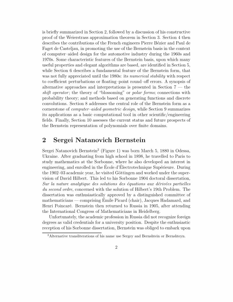
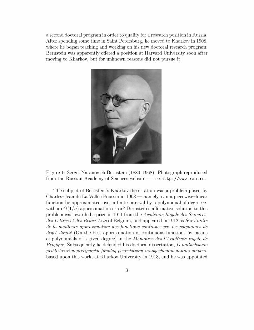
Sergei Natanovich Bernstein2 (Figure 1) was born March 5, 1880 in Odessa,Ukraine. After graduating from high school in 1898, he travelled to Paris tostudy mathematics at the Sorbonne, where he also developed an interest inengineering, and enrolled in the Ecole d’Electrotechnique Superieure. Duringthe 1902–03 academic year, he visited Gottingen and worked under the super-vision of David Hilbert. This led to his Sorbonne 1904 doctoral dissertation,Sur la nature analytique des solutions des equations aux derivees partielles
du second ordre, concerned with the solution of Hilbert’s 19th Problem. Thedissertation was enthusiastically approved by a distinguished committee ofmathematicians — comprising Emile Picard (chair), Jacques Hadamard, andHenri Poincare. Bernstein then returned to Russia in 1905, after attendingthe International Congress of Mathematicians in Heidelberg.
Unfortunately, the academic profession in Russia did not recognize foreigndegrees as valid credentials for a university position. Despite the enthusiasticreception of his Sorbonne dissertation, Bernstein was obliged to embark upon
2Alternative transliterations of his name use Sergey and Bernshtein or Bernshteyn.
2
a second doctoral program in order to qualify for a research position in Russia.After spending some time in Saint Petersburg, he moved to Kharkov in 1908,where he began teaching and working on his new doctoral research program.Bernstein was apparently offered a position at Harvard University soon aftermoving to Kharkov, but for unknown reasons did not pursue it.
Figure 1: Sergei Natanovich Bernstein (1880–1968). Photograph reproducedfrom the Russian Academy of Sciences website — see http://www.ras.ru.
The subject of Bernstein’s Kharkov dissertation was a problem posed byCharles–Jean de La Vallee Poussin in 1908 — namely, can a piecewise–linearfunction be approximated over a finite interval by a polynomial of degree n,with an O(1/n) approximation error? Bernstein’s affirmative solution to thisproblem was awarded a prize in 1911 from the Academie Royale des Sciences,
des Lettres et des Beaux Arts of Belgium, and appeared in 1912 as Sur l’ordre
de la meilleure approximation des fonctions continues par les polynomes de
degre donne (On the best approximation of continuous functions by meansof polynomials of a given degree) in the Memoires des l’Academie royale de
Belgique. Subsequently he defended his doctoral dissertation, O nailuchshem
priblizhenii nepreryvnykh funktsy posredstvom mnogochlenov dannoi stepeni,based upon this work, at Kharkov University in 1913, and he was appointed
3
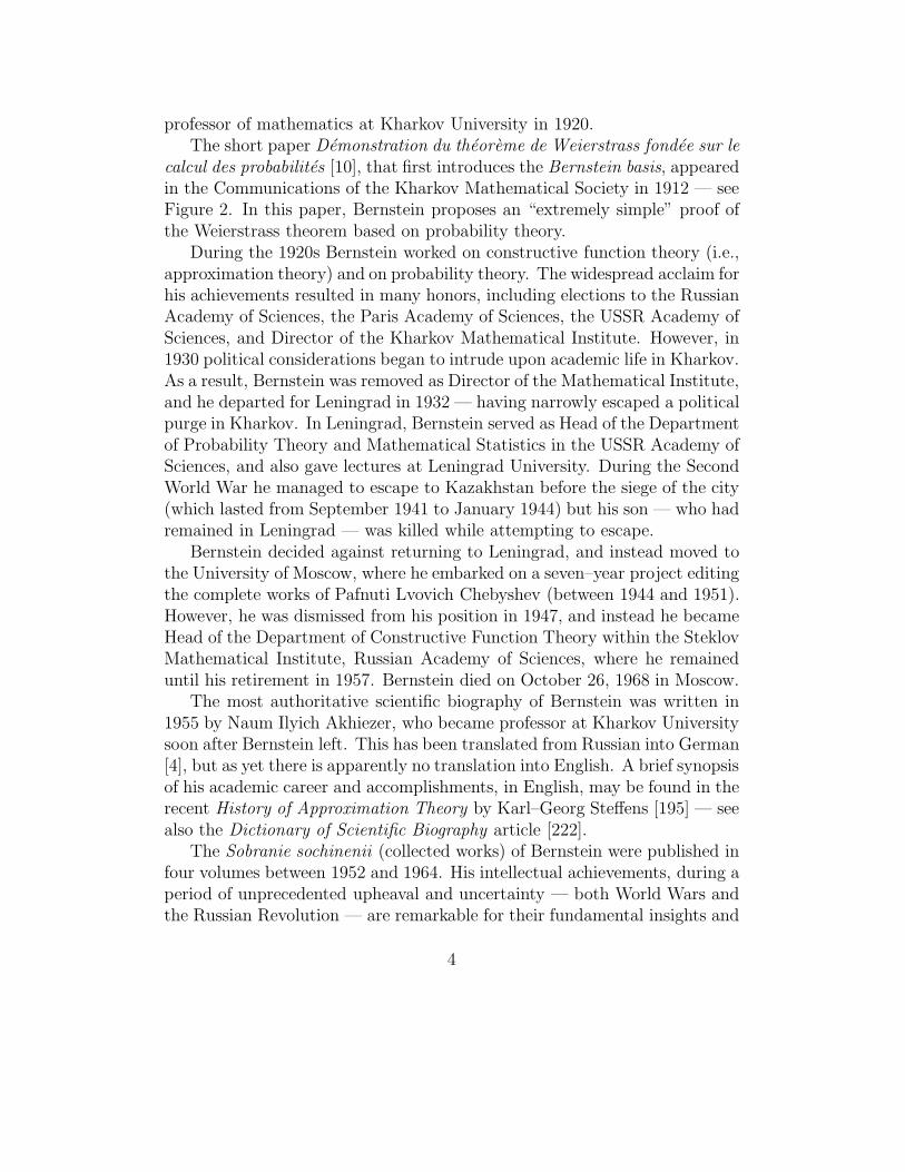
professor of mathematics at Kharkov University in 1920.The short paper Demonstration du theoreme de Weierstrass fondee sur le
calcul des probabilites [10], that first introduces the Bernstein basis, appearedin the Communications of the Kharkov Mathematical Society in 1912 — seeFigure 2. In this paper, Bernstein proposes an “extremely simple” proof ofthe Weierstrass theorem based on probability theory.
During the 1920s Bernstein worked on constructive function theory (i.e.,approximation theory) and on probability theory. The widespread acclaim forhis achievements resulted in many honors, including elections to the RussianAcademy of Sciences, the Paris Academy of Sciences, the USSR Academy ofSciences, and Director of the Kharkov Mathematical Institute. However, in1930 political considerations began to intrude upon academic life in Kharkov.As a result, Bernstein was removed as Director of the Mathematical Institute,and he departed for Leningrad in 1932 — having narrowly escaped a politicalpurge in Kharkov. In Leningrad, Bernstein served as Head of the Departmentof Probability Theory and Mathematical Statistics in the USSR Academy ofSciences, and also gave lectures at Leningrad University. During the SecondWorld War he managed to escape to Kazakhstan before the siege of the city(which lasted from September 1941 to January 1944) but his son — who hadremained in Leningrad — was killed while attempting to escape.
Bernstein decided against returning to Leningrad, and instead moved tothe University of Moscow, where he embarked on a seven–year project editingthe complete works of Pafnuti Lvovich Chebyshev (between 1944 and 1951).However, he was dismissed from his position in 1947, and instead he becameHead of the Department of Constructive Function Theory within the SteklovMathematical Institute, Russian Academy of Sciences, where he remaineduntil his retirement in 1957. Bernstein died on October 26, 1968 in Moscow.
The most authoritative scientific biography of Bernstein was written in1955 by Naum Ilyich Akhiezer, who became professor at Kharkov Universitysoon after Bernstein left. This has been translated from Russian into German[4], but as yet there is apparently no translation into English. A brief synopsisof his academic career and accomplishments, in English, may be found in therecent History of Approximation Theory by Karl–Georg Steffens [195] — seealso the Dictionary of Scientific Biography article [222].
The Sobranie sochinenii (collected works) of Bernstein were published infour volumes between 1952 and 1964. His intellectual achievements, during aperiod of unprecedented upheaval and uncertainty — both World Wars andthe Russian Revolution — are remarkable for their fundamental insights and
4
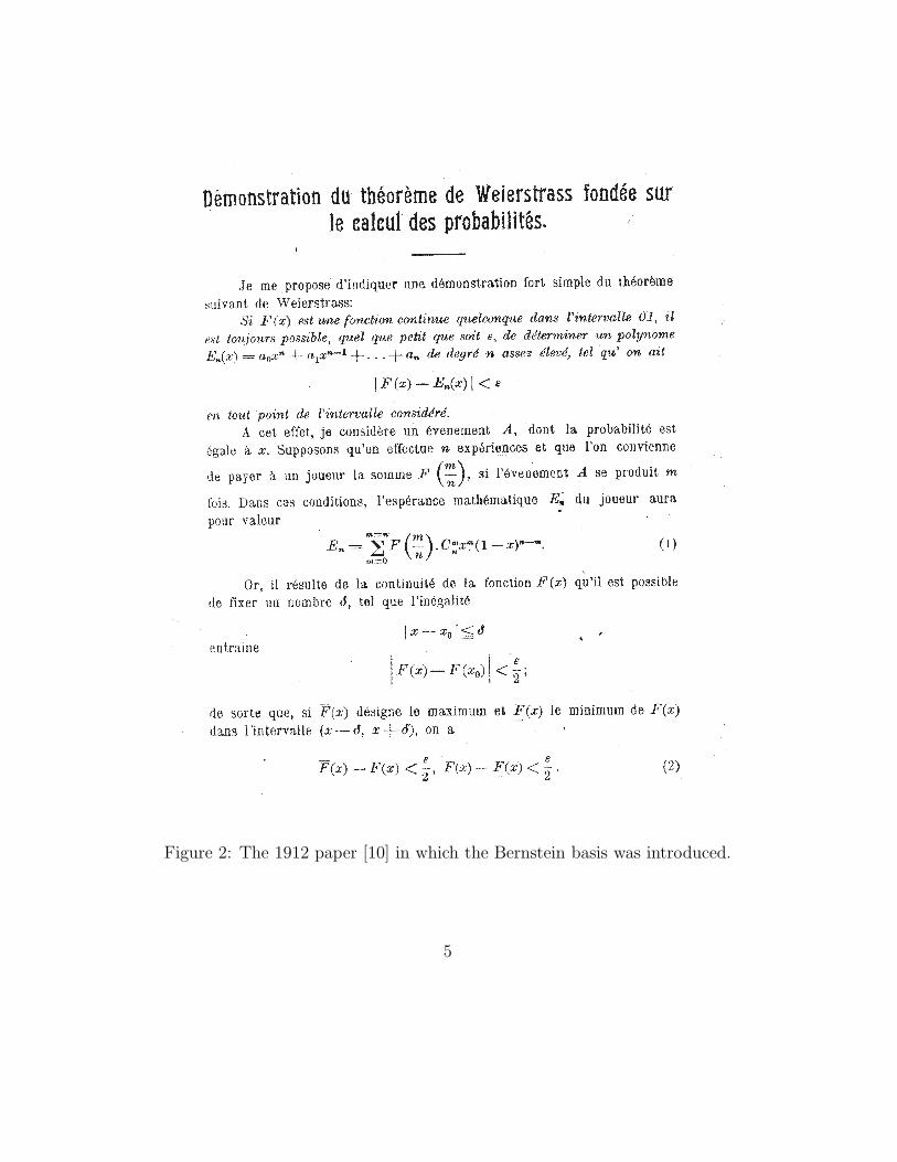
Figure 2: The 1912 paper [10] in which the Bernstein basis was introduced.
5
continuing impact in areas remote from their original contexts.
3 Weierstrass approximation theorem
Polynomials are widely used in computational models of scientific/engineeringproblems, because of their finite evaluation schemes; closure under addition,multiplication, differentiation, integration, and composition; and their abilityto approximate functions that have no closed–form expressions.3 It was theneed to formulate “well–behaved” polynomial approximations that motivatedthe introduction of the Bernstein basis.
3.1 Existence arguments
In 1885 Karl Weierstrass published a proof [213] of what subsequently becameknown as his approximation theorem. This states that, given any continuousfunction f(x) on an interval [ a, b ] and a tolerance ǫ > 0, a polynomial pn(x)of sufficiently high degree n exists, such that
|f(x) − pn(x)| ≤ ǫ for all x ∈ [ a, b ] .
In other words, polynomials can uniformly approximate any function that ismerely continuous over a closed interval. This represents a significant advanceover using the Taylor series expansion to generate polynomial approximationsof a function in two important respects: (a) the function need not be analytic(nor differentiable); and (b) whereas the interval [ a, b ] can be freely specified,the Taylor series must be confined within its radius of convergence — whichcan be difficult to compute. Pinkus [155] describes in detail the contributionsof Weierstrass to approximation theory. As a point of departure for his proof,Weierstrass invokes an integral representation for the function,
f(x) = limk→0
1√πk
∫ +∞
−∞
f(t) exp
[
− (t− x)2
k2
]
dt ,
which may be regarded as its convolution with a Dirac delta function. Otherauthors developed alternative proofs of the approximation theorem, includingarguments based on Fourier series [203], but for the most part these proofswere (a) existential, rather than constructive, in nature; and (b) relied heavilyon analytic limit arguments, rather than concrete algebraic processes.
3Many of these attributes carry over to rational functions (i.e., ratios of polynomials).
6
3.2 Bernstein’s constructive proof
Steffens [195] notes that the Russian school of approximation theory, whichoriginated in the 1850s from Chebyshev’s interest in the design and analysisof mechanical linkages, regarded such existential arguments as rather suspect,and instead emphasized approaches compatible with practical computations(what we now consider algorithms), that can be directly applied to scientificor technical problems. Correspondingly, the distinctive feature of Bernstein’sproof of the Weierstrass theorem, compared to its predecessors, is its explicitconstruction — employing only basic algebraic operations — of a sequence ofpolynomials pn(x) approaching the given function f(x) more closely at everypoint of the interval x ∈ [ a, b ] as the degree n increases.
Since the change of variables specified by t = (x − a)/(b − a) maps x ∈[ a, b ] to t ∈ [ 0, 1 ] without changing the max norm of any function, we canrestrict our attention to continuous functions f(t) on t ∈ [ 0, 1 ] without lossof generality. The Bernstein basis of degree n on t ∈ [ 0, 1 ] is defined by
bnk(t) :=
(n
k
)
(1 − t)n−ktk , k = 0, . . . , n , (1)
and in terms of it the Bernstein polynomial4 associated with any continuousfunction f(t) is specified as
pn(t) :=
n∑
k=0
f(k/n) bnk(t) . (2)
Although pn(t) is nominally of degree n, its actual degree may be less than n(see Section 5.1 below). The uniform convergence of (2) to f(t), as n→ ∞, ispredicated on two fundamental properties of the basis functions (1) — theyare non–negative on t ∈ [ 0, 1 ]; and they form a partition of unity, i.e.,
n∑
k=0
bnk(t) = 1 . (3)
Hence, the value of pn(t), being a sum of sampled values of f(t) at the n+ 1uniformly–spaced ordinates t = k/n weighted by the basis functions bnk(t),
4A number of generalizations of the basic Bernstein polynomial approximation (2), thatpreserve and extend its key properties, have been proposed — see [153, 185, 186, 192, 193].
7
amounts to a convex combination — i.e., a weighted sum, with non–negativeweights that sum to unity — of those sampled values.
It should be noted that, in general, the polynomial approximant (2) doesnot interpolate the sampled values, i.e., pn(k/n) 6= f(k/n). Since the basisfunctions (1) satisfy
bnk(0) =
{
1 if k = 0,
0 if k > 0,bnk(1) =
{
0 if k < n,
1 if k = n,(4)
we always have pn(0) = f(0) and pn(1) = f(1), but the intermediate valuesf(k/n) for 0 < k < n are not interpolated. Moreover (2) does not incorporatethe “polynomial reproduction” property — i.e., pn(t) 6≡ f(t) when f(t) is apolynomial of degree ≤ n, except in the trivial cases n = 0 and 1.
Specifically, when f(t) = c, the fact that pn(t) = c for all n follows fromthe partition–of–unity property (3). Similarly, when f(t) = at+ b, we have
pn(t) = a
n∑
k=0
k
n
(n
k
)
(1 − t)n−ktk + b .
Noting that the k = 0 term of the sum vanishes, and that
k
n
(n
k
)
=
(n− 1
k − 1
)
, (5)
a shift of the summation index yields
pn(t) = atn−1∑
k=0
(n− 1
k
)
(1 − t)n−1−ktk + b ,
and by the partition–of–unity property for the basis of degree n− 1, this issimply at+ b. The ability to exactly reproduce linear (or constant) functionsis called the linear precision property of the Bernstein approximation.
The relation (2) may be regarded as defining an operator that maps anycontinuous function f(t) on [ 0, 1 ] to a polynomial pn(t) of degree ≤ n. Thisoperator is linear, in the sense that if it maps another continuous function g(t)into the polynomial qn(t) of degree ≤ n, then the combination λ f(t)+µ g(t)is mapped into λ pn(t) + µ qn(t). Moreover, as a consequence of the fact thatthe functions (1) are non–negative on [ 0, 1 ] this operator is monotone — i.e.,
8
pn(t) ≥ qn(t) when f(t) ≥ g(t) for t ∈ [ 0, 1 ]. Equivalently, one may say thatit is a positive operator — i.e., pn(t) ≥ 0 when f(t) ≥ 0 for t ∈ [ 0, 1 ].
The conventional modern form of Bernstein’s proof is based on Korovkin’stheorem [125] for positive linear operators: if a polynomial approximant pn(t)to a continuous function f(t) over t ∈ [ 0, 1 ] is specified by a positive linearoperator, its uniform convergence to any continuous function is guaranteedas n → ∞, if one can demonstrate such convergence in the “simple” casesf(t) = 1, t, t2. Since the first two cases are covered by the linear precisionproperty, it is only necessary to consider f(t) = t2, in which case we have
pn(t) =
n∑
k=0
(k
n
)2(n
k
)
(1 − t)n−ktk .
Noting that the k = 0 term vanishes, using the relation (5) again, and shiftingthe summation index, we obtain
pn(t) = t
n−1∑
k=0
k + 1
n
(n− 1
k
)
(1 − t)n−1−ktk = t
(n− 1
nt+
1
n
)
,
where the final expression follows from the linear precision property. Thus,when f(t) = t2 the approximant pn(t) is the quadratic polynomial
pn(t) = t2 +(1 − t)t
n,
and the approximation error is
| f(t) − pn(t) | =(1 − t)t
n.
Since for each t ∈ [ 0, 1 ] this decreases in proportion to 1/n as n increases,pn(t) converges uniformly to f(t). The maximum error is 1/4n, and occursat t = 1
2. More generally, the asymptotic formula
limn→∞
n [ f(t) − pn(t) ] = 12(1 − t)t f ′′(t) (6)
of Voronovskaya [206] holds for t ∈ (0, 1) when f ′′(t) 6= 0. Complete details onthese proofs can be found in standard introductory texts [42, 46, 156, 169] onapproximation theory. Stark [194] traces the history of Bernstein polynomialapproximations, from their introduction in 1912 up to the publication of theclassical treatise by Lorentz [135] in the mid–1950s.
9
3.3 Properties of the approximant
The Bernstein polynomial approximant (2) to a given function f(t) is always“at least as smooth” as f(t). If f(t) has Cr rather than just C0 continuity,all derivatives of pn(t) up to order r converge uniformly to the correspondingderivatives of f(t). A simple demonstration of this convergence may be foundin [88]. Similarly, if bounds on the derivatives of f(t) of each order over [ 0, 1 ]are known, the corresponding derivatives of pn(t) also satisfy those bounds— this implies, for example, that when f(t) is monotone or convex, pn(t) iscorrespondingly monotone or convex (see [46] for complete details).
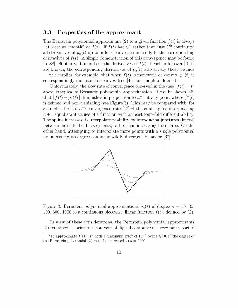
Unfortunately, the slow rate of convergence observed in the case5 f(t) = t2
above is typical of Bernstein polynomial approximation. It can be shown [46]that | f(t)− pn(t) | diminishes in proportion to n−1 at any point where f ′′(t)is defined and non–vanishing (see Figure 3). This may be compared with, forexample, the fast n−4 convergence rate [47] of the cubic spline interpolatingn+1 equidistant values of a function with at least four–fold differentiability.The spline increases its interpolatory ability by introducing junctures (knots)between individual cubic segments, rather than increasing the degree. On theother hand, attempting to interpolate more points with a single polynomialby increasing its degree can incur wildly divergent behavior [67].
Figure 3: Bernstein polynomial approximations pn(t) of degree n = 10, 30,100, 300, 1000 to a continuous piecewise–linear function f(t), defined by (2).
In view of these considerations, the Bernstein polynomial approximants(2) remained — prior to the advent of digital computers — very much part of
5To approximate f(t) = t2 with a maximum error of 10−4 over t ∈ [ 0, 1 ] the degree ofthe Bernstein polynomial (2) must be increased to n = 2500.
10
the theory rather practice of approximations. Notwithstanding their simpleconstruction and orderly convergence properties, it is impractical to employpolynomials with degrees running to hundreds or thousands in “real–world”problems. The eventual widespread adoption of the basis (1) was motivatednot by the approximations (2) of a given function f(t), but by a replacementof the values f(k/n) with freely–specified coefficients ck for k = 0, . . . , n thatcan be used to intuitively manipulate the behavior of the polynomial
p(t) =
n∑
k=0
ckbnk(t) , t ∈ [ 0, 1 ] . (7)
Following past practice [83, 84] we call expression (2) a Bernstein polynomial,while (7) is called a polynomial in Bernstein form. Whereas the former refersto a polynomial approximation of a given function f(t), the latter denotes apolynomial with arbitrary coefficients in the Bernstein basis. Compared tothe familiar monomial or power form of a polynomial,
p(t) =n∑
k=0
aktk , (8)
we shall see that the Bernstein form (7) offers many advantages if one wishesto analyze or manipulate polynomials over a finite interval.
4 De Casteljau and Bezier
As noted in Section 3, the orderly convergence of the Bernstein approximation(2) to a continuous function f(t) as n→ ∞ comes at a severe price: as seen inFigure 3, it proceeds at a very leisurely pace. Philip J. Davis, in his 1963 bookInterpolation and Approximation [46], remarked on the slow convergence ofBernstein approximations as follows:
This fact seems to have precluded any numerical application
of Bernstein polynomials from having been made. Perhaps they
will find application when the properties of the approximant
in the large are of more importance than the closeness of the
approximation.
Coincidentally, two engineers employed in the French automotive industry,Paul de Faget de Casteljau of Citroen and Pierre Etienne Bezier of Renault,became interested in such an application in the early 1960s.
11
4.1 A new application emerges
De Casteljau and Bezier were not concerned with the approximation of givenfunctions, but rather with formulating novel mathematical tools that wouldallow designers to intuitively construct and manipulate complex shapes, suchas automobile bodies, using digital computers. This problem was especiallycritical for “free–form” shapes, that do not admit exact specification througha few simple geometric parameters — centers, axes, angles, dimensions, etc.The motivation was to circumvent the subjective, laborious, and expensiveprocess of sculpting clay models to specify the desired shape.
Although a parametric curve or surface (a vector–valued function of oneor two variables) is an infinitude of points, its computer representation mustemploy just a finite data set. The mapping from the finite set of input valuesto a continuous locus is achieved by interpreting those values as coefficientsfor certain basis functions in the parametric variables. The coefficients mustfurnish natural “shape handles” that permit intuitive creation or modificationof the curve or surface geometry, to satisfy prescribed aesthetic or functionalrequirements. The choice of basis is thus fundamental to a successful designscheme. Ultimately, the work of de Casteljau and Bezier lead to adoption ofthe Bernstein form, typified by what is now called a Bezier curve,
r(t) =
n∑
k=0
pk bnk(t) , t ∈ [ 0, 1 ] , (9)
with control points p0, . . . ,pn as a propitious design scheme. By connectingthe control points we obtain the control polygon, which can be used to analyzeand manipulate the curve shape in a simple and natural manner.
4.2 Paul de Faget de Casteljau
One must bear in mind that, in the early 1960s, digital computers were stillin their infancy, and the goal of exploiting them for shape design would haveseemed far–fetched. De Casteljau, for example, described [56] the reactionat Citroen to this goal as follows:
. . . the designers were astonished and scandalized. Was it
some kind of joke? It was considered nonsense to represent a car
body mathematically. It was enough to please the eye, the word
accuracy had no meaning . . .
12
Citroen’s first attempts at digital shape representation employed a BurroughsE101 computer [56] featuring 128 program steps, a 220–word memory, and a5 kW power consumption! Nevertheless, de Casteljau’s “insane” persistencein pursuing this idea led to the increasing adoption of computer–aided designand manufacturing methods within Citroen from 1963 onward.
De Casteljau’s approach is based on the use of “pilot points” called poles
to define curves and surfaces, a term motivated by the syllabic repetition inthe phrase “interpolation of polynomials with polar forms” (see Section 7.2).Although there is no explicit reference to the Bernstein polynomial basis, keyfeatures of de Casteljau’s courbes et surfaces a poles are unmistakably linkedto it, e.g., the use of barycentric coordinates over intervals and triangles, andthe non–negativity and partition–of–unity properties of the basis functionsassociated with the poles (subsequently identified as Bezier/B–spline controlpoints). However, de Casteljau’s ideas were recorded only in Citroen internaldocuments [51], and remained long unknown to the outside world.
Wolfgang Bohm [27] was instrumental in ensuring that proper credit wasattributed for the eponymous de Casteljau algorithm, the most fundamentalscheme associated with courbes a poles (now commonly called Bezier curves),although it had appeared somewhat earlier [127] in a relatively obscure venue.For a parameter value τ ∈ (0, 1) this algorithm evaluates and subdivides theBezier curve (9), i.e., it computes the curve point r(τ) and the control pointsdefining the “left” and “right” subsegments t ∈ [ 0, τ ] and t ∈ [ τ, 1 ] of r(t) asindividual Bezier curves, over the parameter interval [ 0, 1 ]. Setting p0
j = pj
for j = 0 . . . , n, the algorithm computes a triangular array of points
p00 p0
1 p02 · · p0
n
p11 p1
2 · · p1n
p22 · · p2
n
· · ·
pnn
(10)
defined for j = r, . . . , n and r = 1, . . . , n by the linear interpolations
prj = (1 − τ)pr−1
j−1 + τ pr−1j . (11)
13
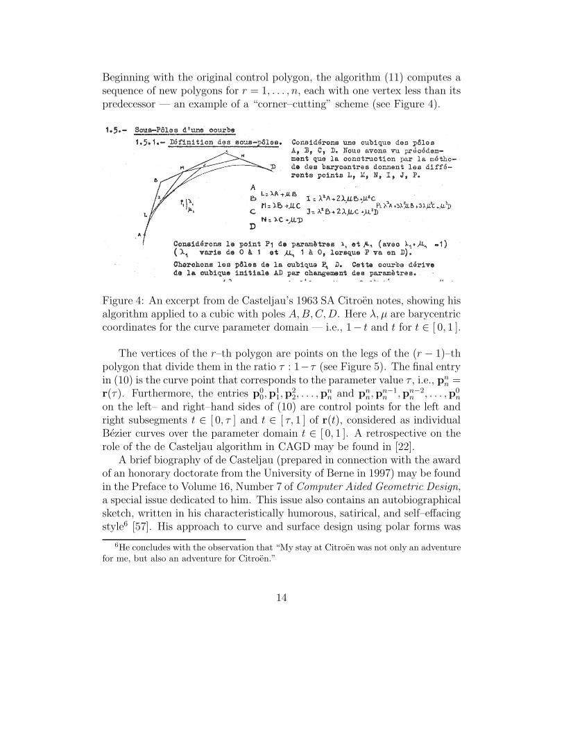
Beginning with the original control polygon, the algorithm (11) computes asequence of new polygons for r = 1, . . . , n, each with one vertex less than itspredecessor — an example of a “corner–cutting” scheme (see Figure 4).
Figure 4: An excerpt from de Casteljau’s 1963 SA Citroen notes, showing hisalgorithm applied to a cubic with poles A,B,C,D. Here λ, µ are barycentriccoordinates for the curve parameter domain — i.e., 1− t and t for t ∈ [ 0, 1 ].
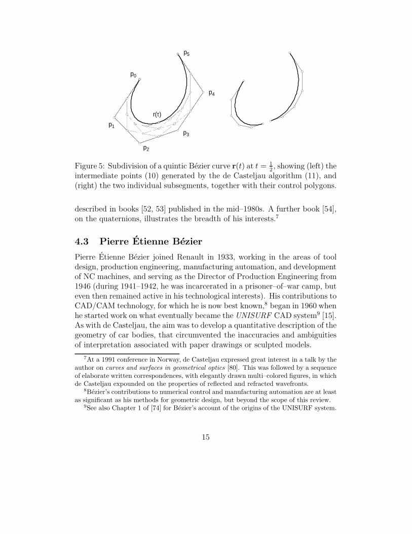
The vertices of the r–th polygon are points on the legs of the (r − 1)–thpolygon that divide them in the ratio τ : 1−τ (see Figure 5). The final entryin (10) is the curve point that corresponds to the parameter value τ , i.e., pn
n =r(τ). Furthermore, the entries p0
0,p11,p
22, . . . ,p
nn and pn
n,pn−1n ,pn−2
n , . . . ,p0n
on the left– and right–hand sides of (10) are control points for the left andright subsegments t ∈ [ 0, τ ] and t ∈ [ τ, 1 ] of r(t), considered as individualBezier curves over the parameter domain t ∈ [ 0, 1 ]. A retrospective on therole of the de Casteljau algorithm in CAGD may be found in [22].
A brief biography of de Casteljau (prepared in connection with the awardof an honorary doctorate from the University of Berne in 1997) may be foundin the Preface to Volume 16, Number 7 of Computer Aided Geometric Design,a special issue dedicated to him. This issue also contains an autobiographicalsketch, written in his characteristically humorous, satirical, and self–effacingstyle6 [57]. His approach to curve and surface design using polar forms was
6He concludes with the observation that “My stay at Citroen was not only an adventurefor me, but also an adventure for Citroen.”
14
r(τ)
p0
p1
p2
p3
p4
p5
Figure 5: Subdivision of a quintic Bezier curve r(t) at t = 12, showing (left) the
intermediate points (10) generated by the de Casteljau algorithm (11), and(right) the two individual subsegments, together with their control polygons.
described in books [52, 53] published in the mid–1980s. A further book [54],on the quaternions, illustrates the breadth of his interests.7
4.3 Pierre Etienne Bezier
Pierre Etienne Bezier joined Renault in 1933, working in the areas of tooldesign, production engineering, manufacturing automation, and developmentof NC machines, and serving as the Director of Production Engineering from1946 (during 1941–1942, he was incarcerated in a prisoner–of–war camp, buteven then remained active in his technological interests). His contributions toCAD/CAM technology, for which he is now best known,8 began in 1960 whenhe started work on what eventually became the UNISURF CAD system9 [15].As with de Casteljau, the aim was to develop a quantitative description of thegeometry of car bodies, that circumvented the inaccuracies and ambiguitiesof interpretation associated with paper drawings or sculpted models.
7At a 1991 conference in Norway, de Casteljau expressed great interest in a talk by theauthor on curves and surfaces in geometrical optics [80]. This was followed by a sequenceof elaborate written correspondences, with elegantly drawn multi–colored figures, in whichde Casteljau expounded on the properties of reflected and refracted wavefronts.
8Bezier’s contributions to numerical control and manufacturing automation are at leastas significant as his methods for geometric design, but beyond the scope of this review.
9See also Chapter 1 of [74] for Bezier’s account of the origins of the UNISURF system.
15
Initially [11, 12] Bezier’s scheme for curve design, like that of de Casteljau,did not explicitly invoke the Bernstein basis. Instead, he used basis functionsfn
1 (t), . . . , fnn (t) characterized by the fact that fn
k (t) increases from 0 to 1 overthe interval t ∈ [ 0, 1 ] and has vanishing derivatives to order k − 1 at t = 0,and to order n− k at t = 1. He showed that fn
k (t) can be expressed as
fnk (t) =
(−1)k
(k − 1)!tk
dk−1
dtk−1
(1 − t)n − 1
t=
n∑
j=k
(−1)j+k
(n
j
)(j − 1
k − 1
)
tj
for k = 1, . . . , n and mischievously attributed this apparently–unknown basisto a fictitious mathematician, Onesime Durand [132]. Bezier specified a curveby an initial point p0 and n vectors a1, . . . , an through the expression
r(t) = p0 +n∑
k=1
akfnk (t) , (12)
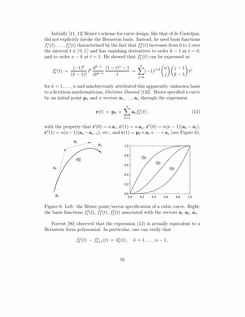
with the property that r′(0) = n a1, r′(1) = n an, r′′(0) = n(n− 1)(a2 − a1),r′′(1) = n(n−1)(an−an−1), etc., and r(1) = p0 +a1 + · · ·+an (see Figure 6).
0.0 0.2 0.4 0.6 0.8 1.00.0
0.2
0.4
0.6
0.8
1.0
p0
a1
a2a3
r(t) f31(t)
f32(t)
f33(t)
Figure 6: Left: the Bezier point/vector specification of a cubic curve. Right:the basis functions f 3
1 (t), f 32 (t), f 3
3 (t) associated with the vectors a1 a2, a3.
Forrest [90] observed that the expression (12) is actually equivalent to aBernstein–form polynomial. In particular, one can verify that
fnk (t) − fn
k+1(t) = bnk(t) , k = 1, . . . , n− 1 ,
16
while 1 − fn1 (t) = bn0 (t) and fn
n (t) = bnn(t), from which one infers that
1 − fnk (t) =
k−1∑
j=0
bnj (t) and fnk (t) =
n∑
j=k
bnj (t)
for k = 1, . . . , n, the partition–of–unity property (3) being invoked to obtainthe latter expression. Thus, substituting for fn
k (t), one finds that the Bezierform (12) is equivalent to the familiar control–point form (9), if we take
pk = p0 +k∑
j=1
aj , k = 1, . . . , n .
Hence, the vectors a1, . . . , an in (12) represent the control polygon legs, i.e.,ak = pk−pk−1 for k = 1, . . . , n. The control–point form (9) is now universallypreferred over the initial–point/vector form (12).
Bezier published his ideas extensively [11, 12, 13, 14, 15, 16, 17, 18] duringthe 1960s and 1970s, and the representation (9) is now conventionally knownas a Bezier curve — although it is closer in spirit to de Casteljau’s formulationthan Bezier’s original formulation. Bezier curves are now a firmly establishedand indispensible tool in computer graphics, engineering design, animation,path planning, and related fields. For example, scalable computer fonts suchas PostScript employ Bezier curves to describe the character shapes.
Bezier retired, after a 42–year career with Renault, in 1975. In additionto degrees in mechanical engineering (1930) and electrical engineering (1931),he received a doctorate in mathematics from the University of Paris (1977).He was also awarded an honorary doctorate from the Technical University ofBerlin, and from 1968 to 1979 served as Professor of Production Engineeringat the Conservatoire National des Arts et Metiers. Bezier remained active inretirement through correspondence, publications, and presentations until hisdeath in 1999. Correspondence of Christophe Rabut with Bezier, describingthe origins of his curve design ideas, shortly before he passed away, may befound in [163]. Finally, a detailed biography of Bezier by Pierre–Jean Laurentand Paul Sablonniere [132] observes that “His art of living consisted in doingeverything seriously without ever taking himself too seriously.”
New ideas establish a firm foothold only if they are taken up and furtherdeveloped by others. Among many publications that played a key role in thisregard, some noteworthy examples are the papers of Forrest [90]; Gordon andRiesenfeld [106]; Lane and Riesenfeld [130]; and Chang and Wu [37].
17
5 Bernstein basis properties
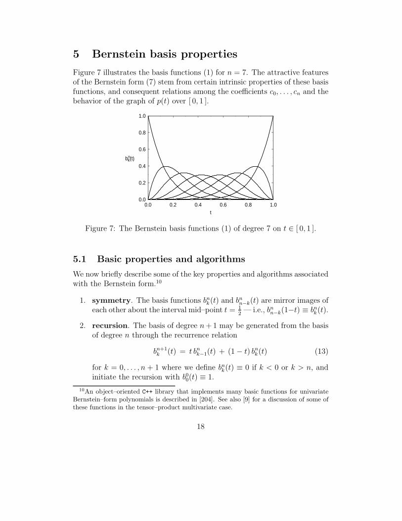
Figure 7 illustrates the basis functions (1) for n = 7. The attractive featuresof the Bernstein form (7) stem from certain intrinsic properties of these basisfunctions, and consequent relations among the coefficients c0, . . . , cn and thebehavior of the graph of p(t) over [ 0, 1 ].
0.0 0.2 0.4 0.6 0.8 1.00.0
0.2
0.4
0.6
0.8
1.0
t
bnk(t)
Figure 7: The Bernstein basis functions (1) of degree 7 on t ∈ [ 0, 1 ].
5.1 Basic properties and algorithms
We now briefly describe some of the key properties and algorithms associatedwith the Bernstein form.10
1. symmetry. The basis functions bnk(t) and bnn−k(t) are mirror images ofeach other about the interval mid–point t = 1
2— i.e., bnn−k(1−t) ≡ bnk(t).
2. recursion. The basis of degree n+ 1 may be generated from the basisof degree n through the recurrence relation
bn+1k (t) = t bnk−1(t) + (1 − t) bnk(t) (13)
for k = 0, . . . , n + 1 where we define bnk(t) ≡ 0 if k < 0 or k > n, andinitiate the recursion with b00(t) ≡ 1.
10An object–oriented C++ library that implements many basic functions for univariateBernstein–form polynomials is described in [204]. See also [9] for a discussion of some ofthese functions in the tensor–product multivariate case.
18
3. non-negativity. As noted in Section 3, the basis functions (1) satisfybnk(t) ≥ 0 for t ∈ [ 0, 1 ]. This property does not hold outside [ 0, 1 ].
4. partition of unity. The property (3) results from the fact that thebasis functions (1) are simply the n+1 terms in the binomial expansionof [ (1 − t) + t ]n. This property is not restricted to [ 0, 1 ].
5. unimodality. bnk(t) has a single extremum, at t = k/n, on t ∈ [ 0, 1 ].Also, for any fixed value t∗ there is a corresponding index k such that
bn0 (t∗) ≤ · · · ≤ bnk−1(t∗) ≤ bnk(t∗) ≥ bnk+1(t∗) ≥ · · · ≥ bnn(t∗) ,
i.e., the values bnk(t∗) are unimodal with respect to the index k. Hence,the control point pk has the greatest influence on the Bezier curve (9)at t = t∗, while the influence of all the other control points diminishesmonotonically as their indices decrease or increase away from k.
6. lower & upper bounds. Properties 3 and 4 imply that for t ∈ [ 0, 1 ]the polynomial (7) satisfies [34, 168] the bounds
min0≤k≤n
ck ≤ p(t) ≤ max0≤k≤n
ck .
7. end–point values. By virtue of the property (4) of the basis functions,the polynomial (7) satisfies p(0) = c0 and p(1) = cn.
8. variation-diminishing property. The number N of real roots of p(t)on t ∈ (0, 1) is less than the number S(c0, . . . , cn) of sign variations inits Bernstein coefficients by an even amount,11
N = S(c0, . . . , cn) − 2k , (14)
for some integer k ≥ 0. This is an expression of Descartes’ Law of Signs[205], since the map t ∈ (0, 1) → u ∈ (0,∞) defined by t(u) = u/(1+u)transforms p(t) into
q(u) = p(t(u)) = (1 + u)−n
n∑
k=0
akuk , where ak =
(n
k
)
ck .
The coefficients ck and ak clearly have the same signs, and roots of q(u)on (0,∞) are in one–to–one correspondence with roots of p(t) on (0, 1).
11When counting the number of sign variations in the sequence of Bernstein coefficients,zeros are ignored. Also, each root on (0, 1) contributes to N according to its multiplicity.
19
9. relation to monomial basis. The Bernstein and monomial (power)bases of degree n are related [83] by the expressions
tk =
n∑
j=k
(j
k
)
(n
k
) bnj (t) , bnk(t) =
n∑
j=k
(−1)j−k
(n
j
)(j
k
)
tj (15)
for k = 0, . . . , n. In particular, case k = 0 of the first expression yieldsthe partition of unity property, while from case k = 1 we obtain
t =bn1 (t) + 2 bn2(t) + · · ·+ n bnn(t)
n,
which induces the linear precision property.
10. scaling the independent variable. The change of variables t → rtmaps the interval [ 0, 1 ] to [ 0, r ]. Setting 1− rt = (1− t) + (1− r)t in
bnk(rt) =
(n
k
)
(1 − rt)n−k(rt)k
and performing a binomial expansion, one can verify that
bnk(rt) =
n∑
j=k
bjk(r) bnj (t) , j = 0, . . . , n . (16)
With r = 12, this allows the Bernstein coefficients of (7) on [ 0, 1
2] — as
generated by mid–point subdivision through the de Casteljau algorithm— to be expressed in terms of the coefficients on [ 0, 1 ]. See (33)–(34)below for the generalization of (16) to an arbitrary interval [ t1, t2 ].
11. derivatives. One can verify that the basis functions (1) satisfy
d
dtbnk(t) = n [ bn−1
k−1(t) − bn−1k (t) ] (17)
where bn−1−1 (t) ≡ 0 and bn−1
n (t) ≡ 0. Substituting into the derivative of(7) and combining terms, we obtain
p′(t) =
n−1∑
k=0
n∆ck bn−1k (t) ,
where ∆ck = ck+1 − ck. Further derivatives can be written in terms ofhigher–order differences of the Bernstein coefficients.
20
12. integrals. By setting n→ n+1 in (17), and adding up and integratinginstances k + 1, . . . , n+ 1 of the resulting equation, we obtain
∫
bnk(t) dt =1
n + 1
n+1∑
j=k+1
bn+1j (t) . (18)
Hence, the indefinite integral of (7) may be expressed as
∫
p(t) dt =
n+1∑
k=1
(
1
n + 1
k−1∑
j=0
cj
)
bn+1k (t) + constant .
Each of the basis functions (1) has the same definite integral, namely1/(n+ 1), and hence
∫ 1
0
p(t) dt =1
n+ 1
n∑
k=0
ck .
13. degree elevation. A polynomial p(t) of true degree n can be expressedin the Bernstein basis of degree n+ r, for all r > 0 — i.e., one can findcoefficients12 cn+r
0 , . . . , cn+rn+r such that (7) can be written as
p(t) =
n+r∑
k=0
cn+rk bn+r
k (t) .
By multiplying (1) with 1 = (1 − t) + t, one can verify that
bnk(t) =
(
1 − k
n+ 1
)
bn+1k (t) +
k + 1
n+ 1bn+1k+1(t) , k = 0, . . . , n ,
and hence by substituting into (7) we obtain
cn+1k =
k
n + 1cnk−1 +
(
1 − k
n+ 1
)
cnk , k = 1, . . . , n ,
while cn+10 = cn0 , cn+1
n+1 = cnn. This defines a unit degree elevation, whichcan be applied repeatedly. The outcome of an r–fold degree elevationmay be determined by multiplying (1) with 1 = [ (1− t)+ t ]r to obtain
bnk(t) =k+r∑
j=k
(nk
)(r
j−k
)
(n+r
j
) bn+rj (t) , k = 0, . . . , n , (19)
12If it is necessary to specify the degree of the Bernstein basis, it appears as a superscripton the coefficients (if no superscript appears, the basis has the default degree n).
21
and substituting into (7) then gives [84]:
cn+rk =
min(n,k)∑
j=max(0,k−r)
(r
k−j
)(nj
)
(n+r
k
) cnj , k = 0, . . . , n+ r .
14. degree reduction. The true degree of a polynomial in Bernstein formis not immediately apparent from its coefficients. The conditions for (7)to be of true degree n−r (with r ≥ 1) are that the power coefficients in(8) must satisfy an = · · · = an−r+1 = 0 6= an−r. These can be expressedin terms of the Bernstein coefficients by noting from (8) and (15) that
ak =k∑
j=0
(−1)k−j
(n
k
)(k
j
)
cj , k = 0, . . . , n .
When these conditions hold, the coefficients in the basis of degree n−rcan be expressed [84] in terms of those in the degree–n basis as
cn−rk =
k∑
j=0
(−1)k−j
(k−j+r−1
r−1
)(nj
)
(n−r
k
) cnj , k = 0, . . . , n− r .
The term degree reduction is also commonly invoked in a looser sense, toconnote best approximation (according to a specified error measure) ofa given polynomial of degree n on [ 0, 1 ] by polynomials of lower degree:see [31, 64, 65, 128, 202, 212]. An interesting fact [136] in this context isthat the polynomial q(t) of degree < n that best approximates (7) — inthese sense of the L2 norm on [ 0, 1 ] — can be identified by minimizingthe sum of squared differences of Bernstein coefficients of p(t) and q(t),when the degree of the latter is elevated to n.
15. arithmetic operations. To add or subtract two polynomials f(t), g(t)of equal degree, one simply adds or subtracts their respective Bernsteincoefficients. If they are of unequal degree, the degrees must be matchedthrough a degree elevation before adding/subtracting the coefficients. Iff(t) and g(t) are degree m and n with Bernstein coefficients a0, . . . , am
and b0, . . . , bn their product f(t)g(t) has [84] the Bernstein coefficients
ck =
min(m,k)∑
j=max(0,k−n)
(mj
)(n
k−j
)
(m+n
k
) ajbk−j , k = 0, . . . , m+ n .
22
In the division f(t)/g(t), the goal is to find the quotient and remainder
polynomials q(t) and r(t) such that f(t) = q(t) g(t)+r(t) with deg(q) =m−n and deg(r) = n−1. Since the long division process for the powerform invokes obvious degree reductions at each step, it does not readilytranslate to the Bernstein basis. Nevertheless, the Bernstein coefficientsq0, . . . , qm−n and r0, . . . , rn−1 of q(t) and r(t) can be determined bycomparing like terms in f(t) = q(t) g(t)+r(t), and solving the resultingsystem of m+ 1 linear equations specified [84] for k = 0, . . . , m by
min(m−n,k)∑
j=max(0,k−n)
(m−n
j
)(n
k−j
)
(mk
) bk−j qj +
min(n−1,k)∑
j=max(0,k−m+n−1)
(m−n+1
k−j
)(n−1
j
)
(mk
) rj = ak .
Minimair [146] describes a more sophisticated division algorithm, withquadratic worst–case cost dependence on the degrees, compared to thecubic worst–case cost of solving the above linear system. See also Buseand Goldman [33], who discuss both division and gcd algorithms.
16. composition. For polynomials f(t) and g(u) of degree m and n withBernstein coefficients a0, . . . , am and b0, . . . .bn the composition problemis concerned with computing the Bernstein coefficients c0, . . . , cmn of thepolynomial p(u) = f(g(u)) defined by substituting t = g(u) in f(t). Anelegant recursive algorithm addressing this problem has been describedby DeRose [59]. This populates a three–dimensional array of values ak
i,j
by first setting a0i,0 = ai for i = 0, . . . , m. Then the expression
aki,j =
1(
knj
)
min(j,kn−n)∑
l=max(0,j−n)
(kn−n
l
)(n
j−l
)[ (1 − bj−l) a
k−1i,l + bj−l a
k−1i+1,l ]
is used for k = 1, . . . , m, i = 0, . . . , m − k, and j = 0, . . . , kn. Finally,the Bernstein coefficients c0, . . . , cmn of p(u) = f(g(u)) are specified by
cj = am0,j , j = 0, . . . , mn .
The generalization to multivariate Bernstein–form polynomials, definedover simplex domains (see Section 8.2), is also presented in [59].
17. interpolation & approximation. There is a unique polynomial p(t)of degree n that interpolates n+1 function values f0, . . . , fn associated
23
with nodes t0, . . . , tn — i.e., p(tk) = fk for k = 0, . . . , n. In power form,p(t) can be obtained by solving the Vandermonde linear system (whichis often ill–conditioned) or by construction of the Lagrange basis for thegiven nodes [46]. For nodes t0, . . . , tn ∈ [ 0, 1 ], on the other hand, theBernstein–Vandermonde system is typically well–conditioned, and canbe solved by accurate and efficient algorithms [58, 140]. Likewise, stableBernstein–basis algorithms have been developed [141] for least–squaresapproximation of the given data by polynomials of degree < n.
18. resultants. The resultant of two polynomials f(t), g(t) is a polynomialexpression in their coefficients, that vanishes if and only if they possessa common root [205], i.e., f(τ) = g(τ) = 0 for some τ ∈ C. Resultantsare typically formulated as determinants, with entries defined in termsof the power coefficients of f(t) and g(t) — e.g., the Sylvester or Bezout
determinants [32]. It has been noted [84, 104] that these determinantscan be expressed in terms of the Bernstein coefficients by replacing eachpower coefficient by the corresponding scaled Bernstein coefficient —i.e., by
(mj
)aj for j = 0, . . . , m and by
(nk
)bk for k = 0, . . . , n. However,
this approach is not optimal in terms of efficiency and stability. Severalalternative resultant formulations have recently been developed by Bini[19, 20] and Winkler [218, 219, 220, 221]. These methods are also usefulin computing greatest common divisors of Bernstein–form polynomials.
Products and ratios of binomial coefficients arise in many algorithms forprocessing Bernstein–form polynomials, and it is desirable to compute theirvalues in exact integer arithmetic, while avoiding the possibility of overflowfor large degrees. Algorithms to efficiently compute the prime decompositions[98, 99] of binomial coefficients are useful in this regard, since they allow theproducts and ratios of binomial coefficients to be determined by the additionor subtraction of corresponding prime exponents.
5.2 Shape features of Bezier curves
The interpretation of some of the above properties, in the case of the Beziercurve (9) and its control polygon, is illustrated in Figure 8 — for completedetails, see [74]. The control polygon may be viewed as a “caricature” of thecurve (9), that exaggerates its shape. However, the correlation between thecurve and control polygon diminishes as the degree n increases: see [149] forbounds on the deviation of the curve from its control polygon.
24
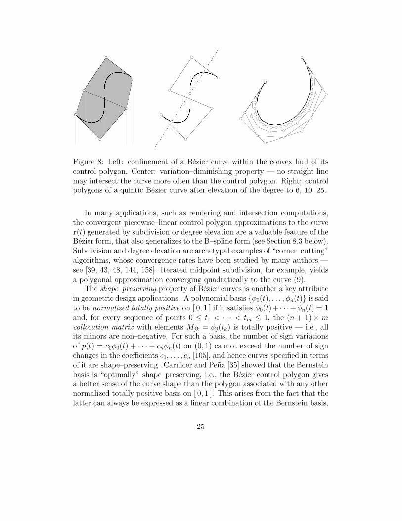
Figure 8: Left: confinement of a Bezier curve within the convex hull of itscontrol polygon. Center: variation–diminishing property — no straight linemay intersect the curve more often than the control polygon. Right: controlpolygons of a quintic Bezier curve after elevation of the degree to 6, 10, 25.
In many applications, such as rendering and intersection computations,the convergent piecewise–linear control polygon approximations to the curver(t) generated by subdivision or degree elevation are a valuable feature of theBezier form, that also generalizes to the B–spline form (see Section 8.3 below).Subdivision and degree elevation are archetypal examples of “corner–cutting”algorithms, whose convergence rates have been studied by many authors —see [39, 43, 48, 144, 158]. Iterated midpoint subdivision, for example, yieldsa polygonal approximation converging quadratically to the curve (9).
The shape–preserving property of Bezier curves is another a key attributein geometric design applications. A polynomial basis {φ0(t), . . . , φn(t)} is saidto be normalized totally positive on [ 0, 1 ] if it satisfies φ0(t)+ · · ·+φn(t) = 1and, for every sequence of points 0 ≤ t1 < · · · < tm ≤ 1, the (n + 1) ×mcollocation matrix with elements Mjk = φj(tk) is totally positive — i.e., allits minors are non–negative. For such a basis, the number of sign variationsof p(t) = c0φ0(t) + · · · + cnφn(t) on (0, 1) cannot exceed the number of signchanges in the coefficients c0, . . . , cn [105], and hence curves specified in termsof it are shape–preserving. Carnicer and Pena [35] showed that the Bernsteinbasis is “optimally” shape–preserving, i.e., the Bezier control polygon givesa better sense of the curve shape than the polygon associated with any othernormalized totally positive basis on [ 0, 1 ]. This arises from the fact that thelatter can always be expressed as a linear combination of the Bernstein basis,
25
specified by a stochastic13 totally positive matrix. See also [142].Although the Bernstein basis is most often used to represent parametric
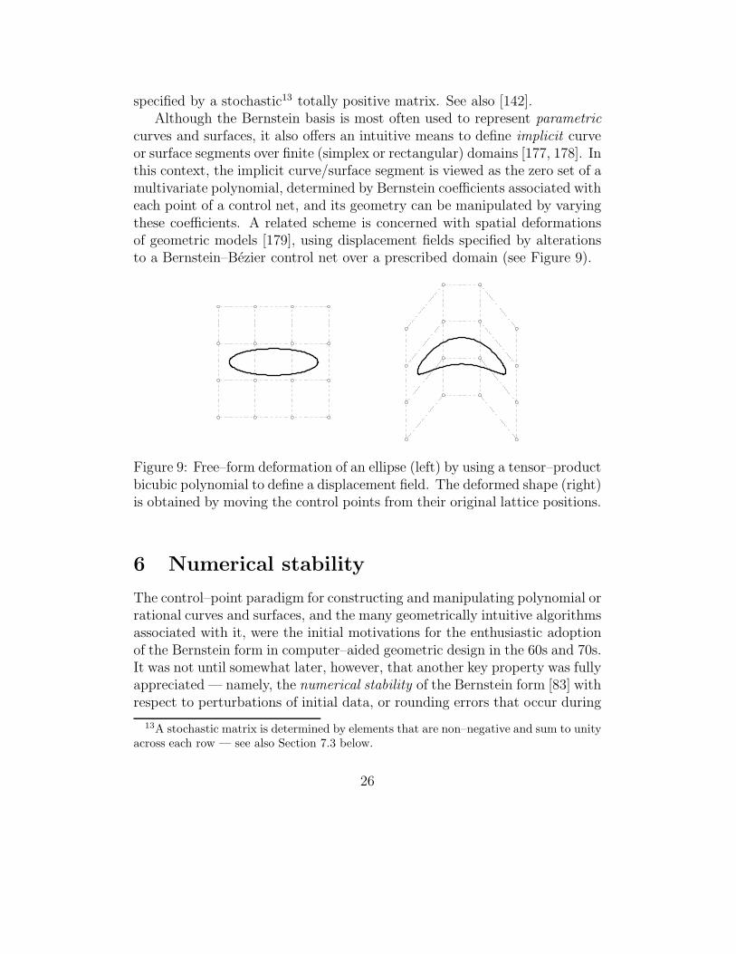
curves and surfaces, it also offers an intuitive means to define implicit curveor surface segments over finite (simplex or rectangular) domains [177, 178]. Inthis context, the implicit curve/surface segment is viewed as the zero set of amultivariate polynomial, determined by Bernstein coefficients associated witheach point of a control net, and its geometry can be manipulated by varyingthese coefficients. A related scheme is concerned with spatial deformationsof geometric models [179], using displacement fields specified by alterationsto a Bernstein–Bezier control net over a prescribed domain (see Figure 9).
Figure 9: Free–form deformation of an ellipse (left) by using a tensor–productbicubic polynomial to define a displacement field. The deformed shape (right)is obtained by moving the control points from their original lattice positions.
6 Numerical stability
The control–point paradigm for constructing and manipulating polynomial orrational curves and surfaces, and the many geometrically intuitive algorithmsassociated with it, were the initial motivations for the enthusiastic adoptionof the Bernstein form in computer–aided geometric design in the 60s and 70s.It was not until somewhat later, however, that another key property was fullyappreciated — namely, the numerical stability of the Bernstein form [83] withrespect to perturbations of initial data, or rounding errors that occur during
13A stochastic matrix is determined by elements that are non–negative and sum to unityacross each row — see also Section 7.3 below.
26
floating–point calculations. The importance of this attribute stems from thehigh premium placed on the “robustness” (i.e., accuracy and consistency) ofthe geometrical computations performed in CAD systems. Unlike most otherforms of scientific or engineering computation, the output of CAD systems —geometric models — are not ends in themselves. Such models are rather thepoint of departure for downstream applications (meshing for finite–elementanalysis, path planning for manufacturing, etc.) that cannot succeed withoutaccurate and consistent geometrical representations.
Any n+1 linearly–independent polynomials φ0(t), . . . , φn(t) of degree ≤ nconstitute a basis for polynomials p(t) of degree n in the variable t, i.e., sucha polynomial can be uniquely specified by coefficients c0, . . . , cn in the form
p(t) =n∑
k=0
ckφk(t) . (20)
When choosing a basis for numerical computations, the sensitivity of p(t) touncertainties in its coefficients is of fundamental concern. Such uncertaintiesmay be regarded as arising from initial measurement error, or — through themethod of backward error analysis [216] — as representing the accumulationof rounding errors during a floating–point computation.
6.1 Condition numbers
Suppose each coefficient ck of (20) suffers a random perturbation δck and p(t)is consequently perturbed to p(t)+δp(t). The magnitude of δp(t) depends on(a) the value of the independent variable t; (b) the statistical distributionsof the perturbations δc0, . . . , δcn; and (c) the adopted basis φ0(t), . . . , φn(t).To focus on the influence of (c), we assume here that (a) t lies on the interval[ 0, 1 ]; and (b) the coefficient perturbations have uniform distributions, witha fixed maximum relative magnitude ǫ, so that
−ǫ ≤ δck/ck ≤ +ǫ (21)
for k = 0, . . . , n. Then the nominal value of (20) is perturbed to
p(t) + δp(t) :=
n∑
k=0
ckφk(t) +
n∑
k=0
δckφk(t) ,
27
where the perturbation δp(t) satisfies the bounds
−n∑
k=0
|δckφk(t)| ≤ δp(t) ≤ +
n∑
k=0
|δckφk(t)| . (22)
Thus, denoting the basis {φ0(t), . . . , φn(t)} by Φ and using (21) we may write
|δp(t)| ≤ CΦ(p(t)) ǫ where CΦ(p(t)) :=
n∑
k=0
|ckφk(t)| . (23)
CΦ(p(t)) is the condition number for the value of the polynomial (20), at eacht, with respect to the uniform relative perturbations (21) of its coefficients inthe basis Φ = {φ0(t), . . . , φn(t)}. It should be noted that CΦ(p(t)) dependson the choice of basis for the representation of p(t).
A basis Φ = {φ0(t), . . . , φn(t)} is said to be non–negative on the intervalt ∈ [ a, b ] if its components satisfy
φk(t) ≥ 0 for t ∈ [ a, b ] , k = 0, . . . , n .
As noted above, the Bernstein basis (1) has this property when [ a, b ] = [ 0, 1 ].Non–negative bases are of interest [81] in the following context.
Theorem 1. Let Ψ = {ψ0(t), . . . , ψn(t)} and Φ = {φ0(t), . . . , φn(t)} be non–
negative bases for polynomials of degree n on t ∈ [ a, b ] such that the former
can be expressed as a non–negative combination of the latter, i.e.,
ψj(t) =
n∑
k=0
Mjkφk(t) , j = 0, . . . , n , (24)
where Mjk ≥ 0 for 0 ≤ j, k ≤ n. Then the condition numbers for the value
of any degree–n polynomial p(t) at any point t ∈ [ a, b ] in these bases satisfy
CΦ(p(t)) ≤ CΨ(p(t)) . (25)
Proof : In the given non–negative bases, let p(t) have the representations
p(t) =
n∑
j=0
ajψj(t) =
n∑
k=0
ckφk(t) . (26)
28
Then, from (24), the coefficients in the two bases must be related by
ck =
n∑
j=0
ajMjk for k = 0, . . . , n . (27)
Since they are both non–negative on t ∈ [ a, b ] the condition numbers for thevalue of p(t) in these bases may be written as
CΦ(p(t)) =
n∑
k=0
|ck|φk(t) and CΨ(p(t)) =
n∑
j=0
|aj |ψj(t) . (28)
Now substituting (27) into CΦ(p(t)) and using the triangle inequality
∣∣∣∣∣
n∑
k=0
xk
∣∣∣∣∣≤
n∑
k=0
|xk| , (29)
we obtain
CΦ(p(t)) =
n∑
k=0
∣∣∣∣∣
n∑
j=0
ajMjk
∣∣∣∣∣φk(t) ≤
n∑
k=0
[n∑
j=0
|ajMjk|]
φk(t) . (30)
Then, setting |ajMjk| = |aj|Mjk (since Mjk ≥ 0 for all j, k) and re–arrangingthe order of summation on the right–hand side of (30), we have
CΦ(p(t)) ≤n∑
j=0
|aj |n∑
k=0
Mjkφk(t) =n∑
j=0
|aj |ψj(t) = CΨ(p(t)) , (31)
where we make use of (24) in the second step.
An important instance of Theorem 1 is the case where Φ is the Bernsteinbasis (1) on [ 0, 1 ] and Ψ is the monomial or “power” basis 1, t, . . . , tn [83].
Corollary 1. The condition numbers CB(p(t)) and CP (p(t)) for the value of
p(t) in the Bernstein and power representations, (7) and (8), satisfy
CB(p(t)) ≤ CP (p(t))
for any polynomial p(t) and any value t ∈ [ 0, 1 ].
29
Proof : The Bernstein and power bases are both non–negative on [ 0, 1 ] andfrom the transformations (15) between them we see that the power basis is anon–negative combination of the Bernstein basis, but not vice–versa. Hence,the conditions of Theorem 1 hold.
In other words, the Bernstein form is systematically more stable than thepower form, when evaluating polynomials on t ∈ [ 0, 1 ] whose coefficients aresubject to the random perturbations (21) of uniform relative magnitude.
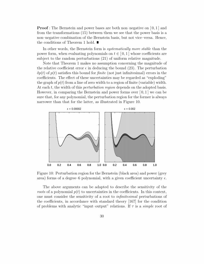
Note that Theorem 1 makes no assumption concerning the magnitude ofthe relative coefficient error ǫ in deducing the bound (23). The perturbationδp(t) of p(t) satisfies this bound for finite (not just infinitesimal) errors in thecoefficients. The effect of these uncertainties may be regarded as “exploding”the graph of p(t) from a line of zero width to a region of finite (variable) width.At each t, the width of this perturbation region depends on the adopted basis.However, in comparing the Bernstein and power forms over [ 0, 1 ] we can besure that, for any polynomial, the perturbation region for the former is alwaysnarrower than that for the latter, as illustrated in Figure 10.
0.0 0.2 0.4 0.6 0.8 1.00.0 0.2 0.4 0.6 0.8 1.0
ε = 0.00002
0.0 0.2 0.4 0.6 0.8 1.00.0 0.2 0.4 0.6 0.8 1.0
ε = 0.002
Figure 10: Perturbation region for the Bernstein (black area) and power (greyarea) forms of a degree–6 polynomial, with a given coefficient uncertainty ǫ.
The above arguments can be adapted to describe the sensitivity of theroots of a polynomial p(t) to uncertainties in the coefficients. In this context,one must consider the sensitivity of a root to infinitesimal perturbations ofthe coefficients, in accordance with standard theory [167] for the conditionof problems with analytic “input–output” relations. If τ is a simple root of
30
(20), i.e., p(τ) = 0 6= p′(τ), then in the limit ǫ → 0 the perturbation δτ ofthe root induced by the perturbations (21) satisfies [96, 97] the bound14
|δτ | ≤ CΦ(τ) ǫ where CΦ(τ) :=1
|p′(τ)|
n∑
k=0
|ckφk(τ)| . (32)
CΦ(τ) is the condition number for the root τ of p(t), in the basis Φ. Sinceit differs from CΦ(p(τ)) only by the factor |p(τ)|−1, which is independent ofthe basis, the result of Theorem 1 applies also to root condition numbers.
Two more important cases of Theorem 1 are concerned with subdivision
and degree elevation of the Bernstein form [83].
Corollary 2. The condition numbers C(p(t)) and C(p(t)) for the value of a
polynomial p(t) of true degree n in the Bernstein bases of degree n+ r and non [ 0, 1 ] satisfy
C(p(t)) ≤ C(p(t))
for any polynomial p(t) and any value t ∈ [ 0, 1 ] and for all r ≥ 1.
Corollary 3. Suppose [ t1, t2 ] ⊂ [ 0, 1 ]. Then the condition numbers C(p(t))and C(p(t)) for the value of a degree–n polynomial p(t) in the Bernstein bases
of degree n on [ t1, t2 ] and [ 0, 1 ] satisfy
C(p(t)) ≤ C(p(t))
for any polynomial p(t) and any value t ∈ [ t1, t2 ].
Corollary 2 follows from the fact that, for all r ≥ 1, the Bernstein basisof degree n is a non–negative combination of the basis of degree n+ r — asexpressed by (19). Similarly, Corollary 3 is a consequence of the fact that,whenever [ t1, t2 ] ⊂ [ 0, 1 ] the Bernstein basis on [ 0, 1 ] can be expressed as anon–negative combination of the basis
bnk(t) =
(n
k
)(t2 − t)n−k(t− t1)
k
(t2 − t1)n, k = 0, . . . , n
on [ t1, t2 ]. Specifically [82], we have
bnj (t) =
n∑
k=0
Mjk bnk(t) , j = 0, . . . , n , (33)
14For an m–fold root, |δτ | grows like ǫ1/m rather than linearly with ǫ, as in (32).
31
where
Mjk =
min(j,k)∑
i=max(0,j+k−n)
bn−kj−i (t1) b
ki (t2) , 0 ≤ j, k ≤ n . (34)
Corollaries 2 and 3 also apply to the root condition numbers.
6.2 Wilkinson polynomial
A “simple” polynomial whose roots are notoriously difficult to compute [215]is the Wilkinson polynomial
p(t) =n∏
k=1
(t− k/n) , n = 20 , (35)
with twenty equidistant roots on the interval t ∈ [ 0, 1 ]. This polynomial wasfirst employed by the British numerical analyst J. H. Wilkinson15 in 1959, inthe context of testing a software implementation of floating–point arithmetic(only fixed–point arithmetic processors were available then). To compute theroots of p(t), Wilkinson first determined its power coefficients a0, . . . , an bymultiplying out (35), and then used the power form to evaluate p(t) and p′(t)for Newton–Raphson iterations. But he found that most of the roots couldnot be determined with more than just a few accurate digits — if at all. Aftereliminating the possibility of bugs in the software, Wilkinson found the truesource of the problem — the extreme sensitivity of the roots to perturbationsin the power coefficients a0, . . . , an. He subsequently called this “the mosttraumatic experience in my career as a numerical analyst” [217].
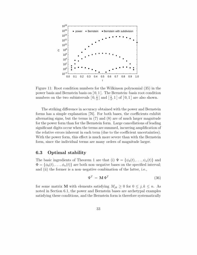
A radically different picture emerges [83] if one uses the Bernstein, ratherthan the power, form of (35). By Theorem 1, we expect the root conditionnumbers in the Bernstein basis to be systematically smaller than those in thepower basis. An explicit computation shows that the difference is substantial:the largest condition numbers are ∼ 1013 in the power basis, but only ∼ 106
in the Bernstein basis [83] — see Figure 11. Typically, the base 10 logarithmof a condition number indicates the number of inaccurate significant decimaldigits one can expect in the result of a floating–point calculation. Thus, withdouble–precision arithmetic (∼ 15 significant digits) one struggles to securejust a few accurate digits in the roots of p(t) with the power form, but theBernstein form typically yields at least 9 accurate digits.
15Wilkinson actually used roots at t = 1, . . . , 20. Scaling them down to the unit intervalt ∈ [ 0, 1 ] as in (35) does not materially alter the problem.
32
0.0 0.1 0.2 0.3 0.4 0.5 0.6 0.7 0.8 0.9 1.010–2
100
102
104
106
108
1010
1012
1014
1016
1018
τ
C
power Bernstein Bernstein with subdivision
Figure 11: Root condition numbers for the Wilkinson polynomial (35) in thepower basis and Bernstein basis on [ 0, 1 ]. The Bernstein–basis root conditionnumbers on the two subintervals [ 0, 1
2] and [ 1
2, 1 ] of [ 0, 1 ] are also shown.
The striking difference in accuracy obtained with the power and Bernsteinforms has a simple explanation [76]. For both bases, the coefficients exhibitalternating signs, but the terms in (7) and (8) are of much larger magnitudefor the power form than for the Bernstein form. Large cancellations of leadingsignificant digits occur when the terms are summed, incurring amplification ofthe relative errors inherent in each term (due to the coefficient uncertainties).With the power form, this effect is much more severe than with the Bernsteinform, since the individual terms are many orders of magnitude larger.
6.3 Optimal stability
The basic ingredients of Theorem 1 are that (i) Ψ = {ψ0(t), . . . , ψn(t)} andΦ = {φ0(t), . . . , φn(t)} are both non–negative bases on the specified interval;and (ii) the former is a non–negative combination of the latter, i.e.,
ΨT = MΦT (36)
for some matrix M with elements satisfying Mjk ≥ 0 for 0 ≤ j, k ≤ n. Asnoted in Section 6.1, the power and Bernstein bases are archetypal examplessatisfying these conditions, and the Bernstein form is therefore systematically
33
more stable than the power form. One is naturally led to ask if other non–negative bases exist, in terms of which the Bernstein basis can be expressed asa non–negative combination, so they are more stable even than the Bernsteinbasis. This question was studied in [81] and it was shown that, in fact, theBernstein basis is “optimally stable” in the sense outlined below.
Let Pn be the set of all non–negative bases for degree–n polynomials on[ 0, 1 ]. The transformation (36) between degree–n polynomial bases by meansof a non–negative matrix M establishes a partial ordering of Pn. Specifically,when Ψ,Φ ∈ Pn and (36) holds for some non–negative matrix M, we writeΦ - Ψ. Since the product of two non–negative matrices is non–negative, thetransitivity condition Ψ - Φ and Φ - Θ =⇒ Ψ - Θ is satisfied.
Now a non–negative matrix has a non–negative inverse if and only if itis the product of a permutation matrix and a positive diagonal matrix [145].Thus, the relations Φ - Ψ and Ψ - Φ are both satisfied if and only if, withsuitable ordering, the elements of Φ are positive multiples of those of Ψ. Inthat case, we write Φ ∼ Ψ. Finally, when Φ - Ψ but Φ 6∼ Ψ we write Φ ≺ Ψ.We say that Φ precedes Ψ when Φ ≺ Ψ, and Φ is similar to Ψ when Φ ∼ Ψ.
The relation - determines a partial ordering of the set Pn of non–negativebases on [ 0, 1 ]. This ordering is only “partial” since bases Φ,Ψ ∈ Pn existsuch that neither the matrix M in (36), nor its inverse, is non–negative —no precedence (or similarity) relation exists between such bases.
A non–negative basis Φ is a minimal basis of Pn if no basis Ψ ∈ Pn exists,such that Ψ ≺ Φ. Note that, since Pn is only partially ordered, there may be— modulo similarity — more than one minimal basis. The following resultsfrom [81] show that such minimal bases are “optimally stable” in the sense ofthe condition numbers defined above (see also [151, 152] for extensions andgeneralizations of these results).
Theorem 2. Any two non–negative bases Φ,Ψ ∈ Pn satisfy
Φ - Ψ ⇐⇒ CΦ(p(t)) ≤ CΨ(p(t))
for every polynomial p(t) and every value t on the unit interval [ 0, 1 ].
Theorem 3. The Bernstein basis is a minimal element of Pn, and it is the
only minimal element for which the basis functions have no roots in (0, 1).
At present, the Bernstein basis is the only known optimally–stable basisin common use. Other minimal bases of Pn can be constructed (see [81] for
34
examples in P2) but the optimal stability may not suffice for their adoption inapplications. A useful basis must admit efficient algorithms for interpolation,approximation, root–finding, shape manipulation, and similar requirements.The Bernstein basis combines optimal stability with a repertoire of versatilealgorithms that address diverse computational requirements.
Remark 1. The optimal numerical stability of the Bernstein basis is closelyrelated, but not identical, to the optimal shape–preserving property discussedin Section 5. The former property is based on a comparison of bases that arenon–negative on [ 0, 1 ] while the latter is concerned with the more restrictivecontext of normalized totally positive bases (i.e., for any set of nodes on [ 0, 1 ]the collocation matrices must have minors that are all non–negative).
6.4 The Legendre basis
In the least–squares approximation of a given function f(t) over t ∈ [ 0, 1 ] bydegree–n polynomials, i.e., in the construction of the polynomial pn(t) thatminimizes the integral
E =
∫ 1
0
[ f(t) − pn(t) ]2 dt , (37)
it is convenient [169] to express pn(t) in terms of an orthogonal basis,
pn(t) =
n∑
k=0
akφk(t) , (38)
characterized by the property
∫ 1
0
φj(t)φk(t) dt =
{
βk if j = k,
0 if j 6= k,(39)
since this allows the coefficients in (38) to be immediately identified as16
ak =1
βk
∫ 1
0
f(t)φk(t) dt . (40)
Moreover, when deg(φk(t)) = k, the approximant (38) exhibits permanence of
coefficients with respect to its degree, i.e., the coefficients a0, . . . , an of pn+1(t)
16See [141] for direct computation of least–squares approximants in the Bernstein basis.
35
agree with those of pn(t), and on increasing the degree we need only computethe new coefficient an+1. The relations (37), (39), (40) can be generalized byinserting a non–negative weight function w(t) in the integrand.
Now the Bernstein basis (1) is clearly not orthogonal with respect to anynon–negative w(t) but it is intimately related to the Legendre polynomials, afamily of classical orthogonal polynomials with w(t) = 1. Key aspects of thisrelation are (i) the simple and intuitive form of the Legendre polynomials inthe Bernstein basis; and (ii) the relative stability of transformations betweenthe Bernstein and Legendre forms (see Section 6.5 below).
To emphasize symmetries, the Legendre polynomials are usually defined[46, 118] on t ∈ [−1,+1 ]. To express them in Bernstein form, however, itis more convenient to use the interval t ∈ [ 0, 1 ]. The Legendre polynomialsLk(t) on [ 0, 1 ] can be generated through the recurrence relation
(k + 1)Lk+1(t) = (2k + 1)(2t− 1)Lk(t) − k Lk−1(t) , (41)
for k = 1, 2, . . ., commencing with L0(t) = 1 and L1(t) = 2t− 1. This gives
L2(t) = 6t2 − 6t+ 1 , L3(t) = 20t3 − 30t2 + 12t− 1 , . . . etc. (42)
These polynomials satisfy (39) with βk = 1/(2k+1). Alternatively, they maybe defined through Rodrigues’ formula
Lk(t) =1
k!
dk
dtk[ (t− 1)t ]k . (43)
From this formula, the following result can be easily proved by induction —see [78, 133] for complete details of the proof.
Lemma 1. The Legendre polynomial Lk(t) can be expressed in the Bernstein
basis bk0(t), . . . , bkk(t) of degree k as
Lk(t) =
k∑
i=0
(−1)k+i
(k
i
)
bki (t) . (44)
The Bernstein form (44) offers a simple and intuitive characterization ofthe Legendre polynomials, easier to remember than the recurrence relation(41) or Rodrigues’ formula (43) — namely, the Bernstein coefficients of Lk(t)are simply the ordered sequence of binomial coefficients of order k taken withalternating signs (starting with a + or − sign according to whether k is even
36
or odd). The control polygon associated with these coefficients offers usefulinsight into the behavior of the graph of Lk(t) for t ∈ [ 0, 1 ].
Another approach to least–squares approximation using polynomials inBernstein form is to formulate the dual basis functions dn
0 (t), . . . , dnn(t) which
are characterized by the property
∫ 1
0
bnk(t) dnj (t) dt = δjk =
{
1 if j = k,
0 if j 6= k.
Juttler [119] has shown that, when the dual basis functions are themselvesexpressed in Bernstein form as
dnj (t) =
n∑
k=0
ajkbnk(t) ,
the coefficients ajk for 0 ≤ j, k ≤ n are given by
ajk =(−1)j+k
(n
j
)(n
k
)
min(j,k)∑
i=0
(2i+ 1)
(n+ i+ 1
n− j
)(n− i
n− j
)(n+ i+ 1
n− k
)(n− i
n− k
)
.
The polynomial pn(t) minimizing (37) then has the Bernstein coefficients
ck =
∫ 1
0
f(t) dnk(t) dt , k = 0, . . . , n .
Details on conversions between the Bernstein basis and other orthogonalpolynomial bases may be found in [29, 40, 160, 161, 162].
6.5 Basis transformations
In theoretical discussions, the monomial form (8) of a polynomial p(t) is mostfrequently used. In problems of min–max or least–squares approximation, onthe other hand, use of an orthogonal (e.g., Chebyshev or Legendre) basis maybe more convenient. As emphasized above, the Bernstein form is best suitedto manipulating the graph of a polynomial over a finite domain, to achievecertain desired shape properties. In principle, one may freely switch betweenalternative representations, since a change of basis for degree–n polynomials
37
corresponds to a linear map, i.e., an (n+1)× (n+1) matrix, that determinesthe coefficients in the new basis from those in the old basis.
Such basis transformations should generally be avoided if one wishes tofully exploit the stability of the Bernstein form, since they may themselvesincur amplification of relative errors in the coefficients. In other words, theproblem should be formulated ab initio in the Bernstein form, and subsequentcomputations should be performed exclusively in that basis. All the familiarpolynomial operations, typically performed using the power representation,have straightforward Bernstein–form analogs [84].
The stability of transformations between the Bernstein and other baseshas been studied by several authors [44, 75, 78, 109, 133]. It may be quantifiedby a condition number for the matrix that relates the coefficients in the twobases. The p–norm of a vector v = (v0, . . . , vn)T is defined by
‖v‖p :=
[n∑
i=0
|vi|p]1/p
. (45)
In particular, ‖v‖1 = |v0| + · · · + |vn|, ‖v‖2 =√
v20 + · · ·+ v2
n, and ‖v‖∞ =max(|v0|, . . . , |vn|). The matrix norm subordinate to (45) is defined by
‖M‖p := maxv 6=0
‖Mv‖p
‖v‖p
. (46)
Specifically, ‖M‖1 and ‖M‖∞ are the greatest of the column sums and rowsums of absolute values of the matrix elements, respectively, while ‖M‖2 =√λmax, where λmax is the largest eigenvalue of MTM [196]. Now if the matrix
M maps x = (x0, . . . , xn)T to y = (y0, . . . , yn)T according to
y = Mx , (47)
and a perturbation δx = (δx0, . . . , δxn) of the “input” induces a perturbationδy = (δy0, . . . , δyn) of the “output,” the magnitudes of these perturbationsmay be characterized by the fractional measures
ǫx :=‖δx‖p
‖x‖p
and ǫy :=‖δy‖p
‖y‖p
. (48)
One can then show [196] that ǫy is bounded in terms of ǫx by the relation
ǫy ≤ Cp(M) ǫx , Cp(M) := ‖M‖p‖M−1‖p , (49)
38
Cp(M) being the p–norm condition number of M. The bound in (49) is sharp
— i.e., a perturbation δx exists for which (49) holds with equality.For transformations between the Bernstein and power forms, the elements
of M and M−1 are defined by the relations (15) and one can show17 [75] that
C1(M) = C∞(M) = (n+ 1)
(n
ν
)
2 ν , ν =
⌊2(n+ 1)
3
⌋
. (50)
The simpler form 3n+1√
(n+ 1)/4π is an excellent approximation [75].
100
105
1010
1015
1020
1025
0 5 10 15 20 25 30polynomial degree n
cond
ition
num
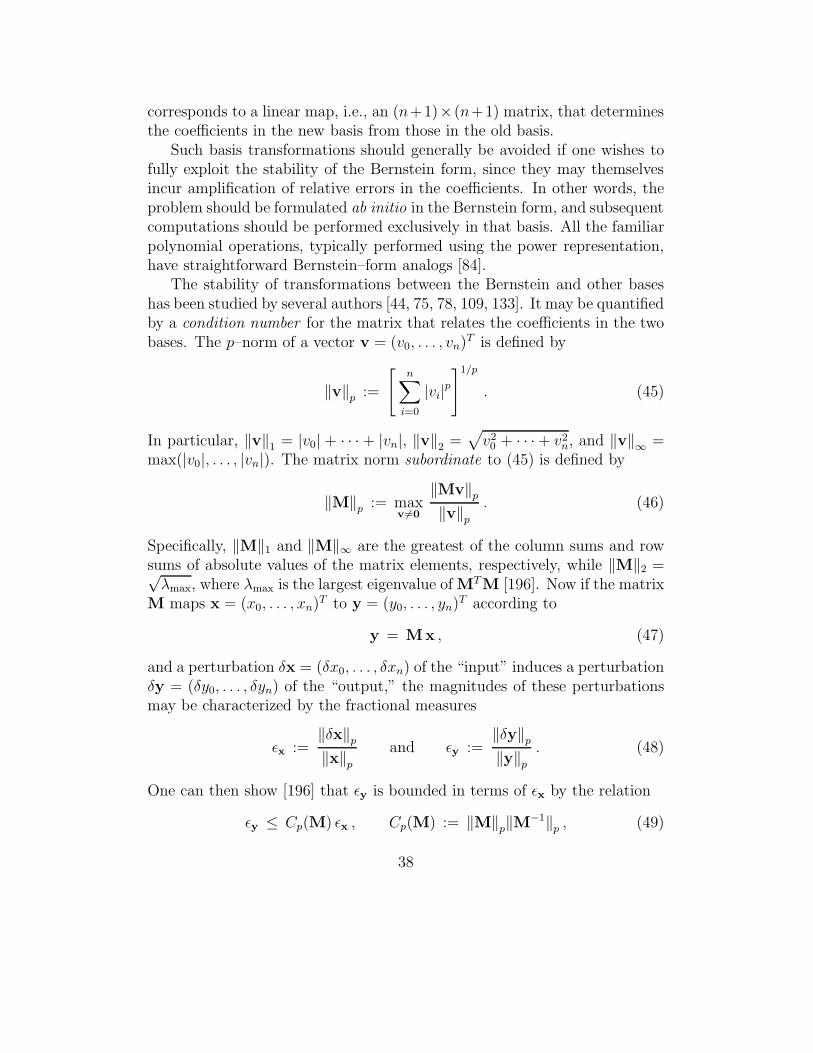
ber
Figure 12: Condition numbers for transformations between polynomial bases— Bernstein–Legendre (squares p = 1, and circles p = ∞); Bernstein–power(triangles, both p = 1 and ∞); and Bernstein–Hermite (diamonds p = ∞).
Figure 12 illustrates the growth of the condition number with degree n fortransformations among the power, Legendre, Hermite, and Bernstein bases,in the p = 1 and p = ∞ norms. The Legendre–Bernstein transformation (seeSection 6.4 above) is comparatively well–conditioned. The power–Bernsteintransformation condition number (50) exhibits a faster growth, although notas severe as transformations that involve the Hermite form.
Since subdivision plays a fundamental role in algorithms for Bernstein–form polynomials, it is also important to characterize the stability of the map
17The “floor” function ⌊x⌋ indicates the largest integer not exceeding x.
39
that relates the coefficients c0, . . . , cn in the Bernstein basis on a sub–interval[ t1, t2 ] to the coefficients c0, . . . , cn on the interval [ 0, 1 ]. In [82] it was shownthat this map may be specified by
cj =n∑
k=0
Mjkck , j = 0, . . . , n ,
where the elements Mjk of the (n + 1) × (n + 1) matrix M are defined by
Mjk =
min(j,k)∑
i=max(0,j+k−n)
bn−jk−i (t1) b
ji (t2) , 0 ≤ j, k ≤ n .
Setting tm = 12(t1 + t2), the condition number of this matrix in the p = ∞
norm may be expressed [82] as
C∞(M) =
[2 max(tm, 1 − tm)
t2 − t1
]n
.
See also [120] for a rounding–error analysis of the de Casteljau algorithm.
7 Alternative approaches
The versatility of the Bernstein form is evident in the wide variety of availableapproaches for elucidating the algorithms and properties associated with it.Some alternative paradigms are summarized here, based on the shift operator,polar forms (or blossoms), connections to probability theory, and the use ofgenerating functions and discrete convolutions.
7.1 The shift operator
Many properties and algorithms associated with the Bernstein form (7) canbe easily derived by invoking a “shift operator” S, whose action on a sequenceof Bernstein coefficients c0, . . . , cn is such as to increment each subscript by1. In this context, we allow the subscripts to assume all integer values, i.e.,we consider the infinite sequence
. . . , c−1, c0, c1, . . . , cn−1, cn, cn+1, . . . ,
40
where it is understood that ck = 0 if k < 0 or > n. As a short–hand notation,we write
Sck = ck+1 , (51)
and correspondingly Srck = ck+r. An inverse S−1 can also be defined, thatdecrements each subscript by 1, indicated by the notation by S−1ck = ck−1,so that S−1 acting on Sck (or S on S−1ck) yields ck. Finally, we also definethe identity operator I = S0, which leaves subscripts unchanged.
Consider now the operator expression (1− t) I + tS for any real value t.By the binomial theorem, its n–th power may be formally expanded as
[ (1 − t) I + tS ]n =
n∑
k=0
(n
k
)
(1 − t)n−ktk Sk =
n∑
k=0
bnk(t)Sk .
Hence, the polynomial (7) may be represented by the compact expression
p(t) = [ (1 − t) I + tS ]n c0 . (52)
Since the first forward differences of the coefficients are ∆ck = ck+1 − ck, weintroduce the operator
∆ = S − I ,and (52) can alternatively be written as
p(t) = [ I + t∆ ]n c0 .
By way of example, we illustrate the use of (52) to obtain the derivativeand integral of (7). The derivative of [ (1− t) I + tS ]n with respect to t maybe expressed as
d
dt[ (1 − t) I + tS ]n = n [ (1 − t) I + tS ]n−1∆ . (53)
Thus, by writing
p′(t) = n [ (1 − t) I + tS ]n−1∆c0 , (54)
and noting that Sk∆c0 = Sk(c1 − c0) = ck+1 − ck = ∆ck, we obtain
p′(t) =n−1∑
k=0
n∆ck
(n− 1
k
)
(1 − t)n−1−ktk =n−1∑
k=0
n∆ckbn−1k (t)
41
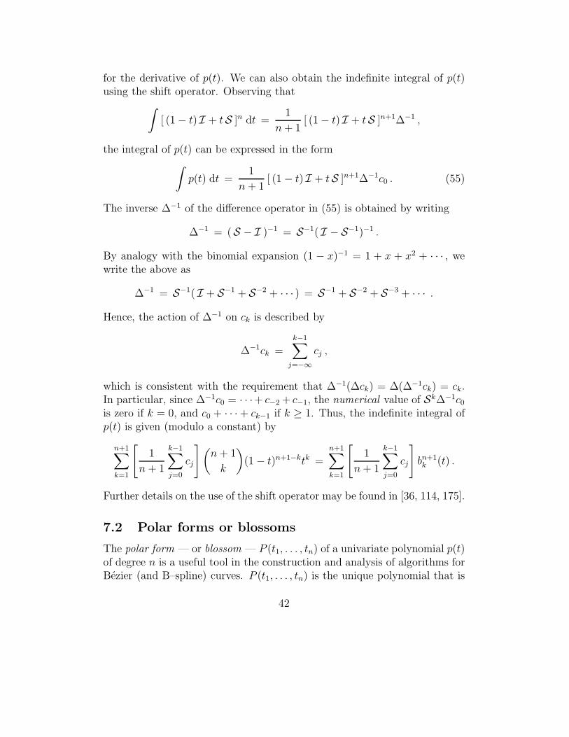
for the derivative of p(t). We can also obtain the indefinite integral of p(t)using the shift operator. Observing that
∫
[ (1 − t) I + tS ]n dt =1
n+ 1[ (1 − t) I + tS ]n+1∆−1 ,
the integral of p(t) can be expressed in the form
∫
p(t) dt =1
n + 1[ (1 − t) I + tS ]n+1∆−1c0 . (55)
The inverse ∆−1 of the difference operator in (55) is obtained by writing
∆−1 = (S − I )−1 = S−1( I − S−1)−1 .
By analogy with the binomial expansion (1 − x)−1 = 1 + x + x2 + · · · , wewrite the above as
∆−1 = S−1( I + S−1 + S−2 + · · · ) = S−1 + S−2 + S−3 + · · · .
Hence, the action of ∆−1 on ck is described by
∆−1ck =k−1∑
j=−∞
cj ,
which is consistent with the requirement that ∆−1(∆ck) = ∆(∆−1ck) = ck.In particular, since ∆−1c0 = · · ·+ c−2 + c−1, the numerical value of Sk∆−1c0is zero if k = 0, and c0 + · · · + ck−1 if k ≥ 1. Thus, the indefinite integral ofp(t) is given (modulo a constant) by
n+1∑
k=1
[
1
n + 1
k−1∑
j=0
cj
](n + 1
k
)
(1 − t)n+1−ktk =
n+1∑
k=1
[
1
n+ 1
k−1∑
j=0
cj
]
bn+1k (t) .
Further details on the use of the shift operator may be found in [36, 114, 175].
7.2 Polar forms or blossoms
The polar form — or blossom — P (t1, . . . , tn) of a univariate polynomial p(t)of degree n is a useful tool in the construction and analysis of algorithms forBezier (and B–spline) curves. P (t1, . . . , tn) is the unique polynomial that is
42
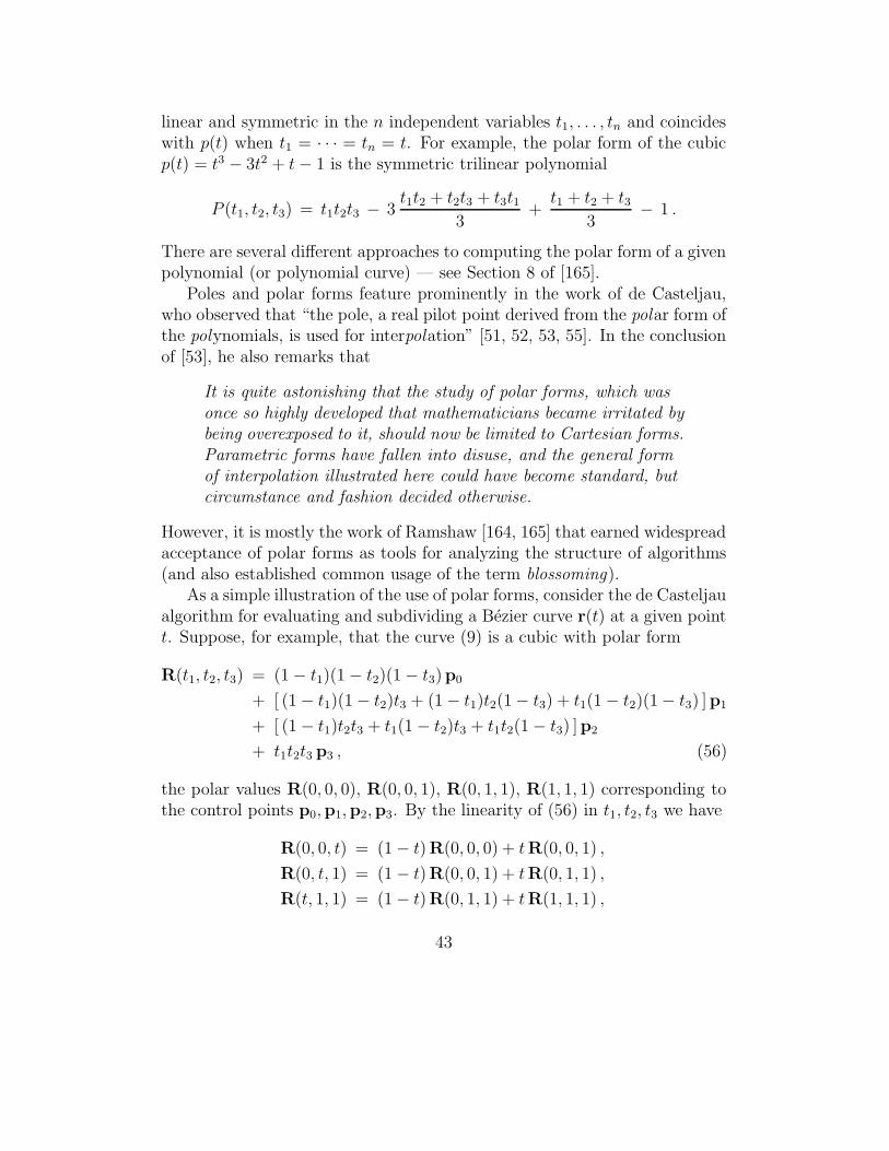
linear and symmetric in the n independent variables t1, . . . , tn and coincideswith p(t) when t1 = · · · = tn = t. For example, the polar form of the cubicp(t) = t3 − 3t2 + t− 1 is the symmetric trilinear polynomial
P (t1, t2, t3) = t1t2t3 − 3t1t2 + t2t3 + t3t1
3+t1 + t2 + t3
3− 1 .
There are several different approaches to computing the polar form of a givenpolynomial (or polynomial curve) — see Section 8 of [165].
Poles and polar forms feature prominently in the work of de Casteljau,who observed that “the pole, a real pilot point derived from the polar form ofthe polynomials, is used for interpolation” [51, 52, 53, 55]. In the conclusionof [53], he also remarks that
It is quite astonishing that the study of polar forms, which was
once so highly developed that mathematicians became irritated by
being overexposed to it, should now be limited to Cartesian forms.
Parametric forms have fallen into disuse, and the general form
of interpolation illustrated here could have become standard, but
circumstance and fashion decided otherwise.
However, it is mostly the work of Ramshaw [164, 165] that earned widespreadacceptance of polar forms as tools for analyzing the structure of algorithms(and also established common usage of the term blossoming).
As a simple illustration of the use of polar forms, consider the de Casteljaualgorithm for evaluating and subdividing a Bezier curve r(t) at a given pointt. Suppose, for example, that the curve (9) is a cubic with polar form
R(t1, t2, t3) = (1 − t1)(1 − t2)(1 − t3)p0
+ [ (1 − t1)(1 − t2)t3 + (1 − t1)t2(1 − t3) + t1(1 − t2)(1 − t3) ]p1
+ [ (1 − t1)t2t3 + t1(1 − t2)t3 + t1t2(1 − t3) ]p2
+ t1t2t3 p3 , (56)
the polar values R(0, 0, 0), R(0, 0, 1), R(0, 1, 1), R(1, 1, 1) corresponding tothe control points p0,p1,p2,p3. By the linearity of (56) in t1, t2, t3 we have
R(0, 0, t) = (1 − t)R(0, 0, 0) + tR(0, 0, 1) ,
R(0, t, 1) = (1 − t)R(0, 0, 1) + tR(0, 1, 1) ,
R(t, 1, 1) = (1 − t)R(0, 1, 1) + tR(1, 1, 1) ,
43
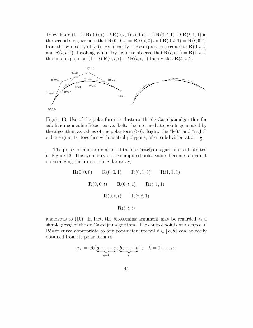
To evaluate (1− t)R(0, 0, t)+ tR(0, t, 1) and (1− t)R(0, t, 1)+ tR(t, 1, 1) inthe second step, we note that R(0, 0, t) = R(0, t, 0) and R(0, t, 1) = R(t, 0, 1)from the symmetry of (56). By linearity, these expressions reduce to R(0, t, t)and R(t, t, 1). Invoking symmetry again to observe that R(t, t, 1) = R(1, t, t)the final expression (1 − t)R(0, t, t) + tR(t, t, 1) then yields R(t, t, t).
R(0,0,0)
R(0,0,1)
R(0,1,1)
R(1,1,1)R(0,0,t)
R(0,t,1)
R(t,1,1)
R(0,t,t)
R(t,t,1)R(t,t,t)
Figure 13: Use of the polar form to illustrate the de Casteljau algorithm forsubdividing a cubic Bezier curve. Left: the intermediate points generated bythe algorithm, as values of the polar form (56). Right: the “left” and “right”cubic segments, together with control polygons, after subdivision at t = 1
2.
The polar form interpretation of the de Casteljau algorithm is illustratedin Figure 13. The symmetry of the computed polar values becomes apparenton arranging them in a triangular array,
R(0, 0, 0) R(0, 0, 1) R(0, 1, 1) R(1, 1, 1)
R(0, 0, t) R(0, t, 1) R(t, 1, 1)
R(0, t, t) R(t, t, 1)
R(t, t, t)
analogous to (10). In fact, the blossoming argument may be regarded as asimple proof of the de Casteljau algorithm. The control points of a degree–nBezier curve appropriate to any parameter interval t ∈ [ a, b ] can be easilyobtained from its polar form as
pk = R( a , . . . , a︸ ︷︷ ︸
n−k
, b , . . . , b︸ ︷︷ ︸
k
) , k = 0, . . . , n .
44
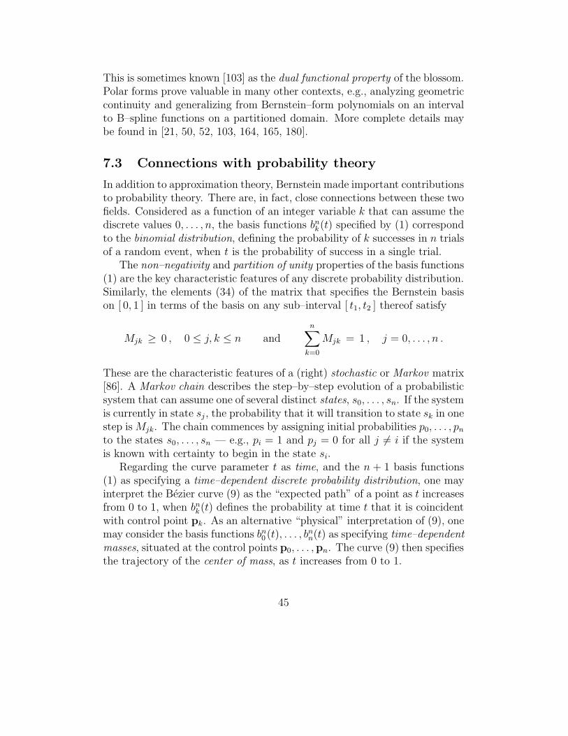
This is sometimes known [103] as the dual functional property of the blossom.Polar forms prove valuable in many other contexts, e.g., analyzing geometriccontinuity and generalizing from Bernstein–form polynomials on an intervalto B–spline functions on a partitioned domain. More complete details maybe found in [21, 50, 52, 103, 164, 165, 180].
7.3 Connections with probability theory
In addition to approximation theory, Bernstein made important contributionsto probability theory. There are, in fact, close connections between these twofields. Considered as a function of an integer variable k that can assume thediscrete values 0, . . . , n, the basis functions bnk(t) specified by (1) correspondto the binomial distribution, defining the probability of k successes in n trialsof a random event, when t is the probability of success in a single trial.
The non–negativity and partition of unity properties of the basis functions(1) are the key characteristic features of any discrete probability distribution.Similarly, the elements (34) of the matrix that specifies the Bernstein basison [ 0, 1 ] in terms of the basis on any sub–interval [ t1, t2 ] thereof satisfy
Mjk ≥ 0 , 0 ≤ j, k ≤ n andn∑
k=0
Mjk = 1 , j = 0, . . . , n .
These are the characteristic features of a (right) stochastic or Markov matrix[86]. A Markov chain describes the step–by–step evolution of a probabilisticsystem that can assume one of several distinct states, s0, . . . , sn. If the systemis currently in state sj , the probability that it will transition to state sk in onestep is Mjk. The chain commences by assigning initial probabilities p0, . . . , pn
to the states s0, . . . , sn — e.g., pi = 1 and pj = 0 for all j 6= i if the systemis known with certainty to begin in the state si.
Regarding the curve parameter t as time, and the n + 1 basis functions(1) as specifying a time–dependent discrete probability distribution, one mayinterpret the Bezier curve (9) as the “expected path” of a point as t increasesfrom 0 to 1, when bnk(t) defines the probability at time t that it is coincidentwith control point pk. As an alternative “physical” interpretation of (9), onemay consider the basis functions bn0 (t), . . . , bnn(t) as specifying time–dependent
masses, situated at the control points p0, . . . ,pn. The curve (9) then specifiesthe trajectory of the center of mass, as t increases from 0 to 1.
45
For a comprehensive discussion of the connections between probabilitytheory, Markov chains, and polynomial bases that provide intuitive geometricdesign schemes, see the articles by Goldman [100, 101, 102] and also [106].
7.4 Generating functions & discrete convolutions
According to Wilf [214], a generating function is “a clothesline on which wehang up a sequence of numbers for display.” More specifically, the sequenceof numbers a0, a1, a2, . . . is considered to be the coefficients in the power seriesexpansion a0 + a1x+ a2x
2 + · · · of a generating function f(x).This idea can also be generalized to specify a generating function for a
sequence of functions φ0(t), φ1(t), φ2(t), . . . by considering these functions tobe the coefficients in the power series expansion of a bivariate function f(t, x)with respect to x, i.e.,
f(t, x) =
∞∑
k=0
φk(t) xk .
The generating function can prove useful in determining various properties,identities, and recurrence relations for φ0(t), φ1(t), φ2(t), . . . When f(t, x) isa polynomial, a simple generating function [103] for the Bernstein basis is
f(t, x) = (1 − t+ tx)n =n∑
k=0
bnk(t) xk .
Simsek [187] considers a generalization of the Bernstein basis, defined by
bnk,s(t) =
(n
ks
)(1 − t)n−kstks
2k(s−1),
which specializes to (1) when s = 1. This basis can be obtained from thegenerating function expansion
fk,s(t, x) =2k(1
2tx)kse(1−t)x
(ks)!=
∞∑
n=0
bnk,s(t)xn
n!, (57)
where it is understood that bnk,s(t) ≡ 0 if ks > n. For the case s = 1 of the“ordinary” Bernstein basis (1), with bnk(t) ≡ 0 if k > n, this reduces to
fk(t, x) =(tx)ke(1−t)x
k!=
∞∑
n=0
bnk(t)xn
n!. (58)
46
Note that this generates basis functions of fixed index k and increasing degreen, rather than vice–versa. The generating functions (57)–(58) are employedin [187, 188, 189] to derive various basic properties of the Bernstein form.
Another approach to analyzing properties of the Bernstein form is throughthe interpretation that the basis (1) arises from a discrete convolution — seeGoldman [103]. The discrete convolution
C = A⊗ B = {c0(t), . . . , cm+n(t)}
of two function sequences A = {a0(t), . . . , am(t)} and B = {b0(t), . . . , bn(t)}is the function sequence specified by
ck(t) =∑
i+j=k
ai(t)bj(t) .
The degree–n Bernstein basis (1) can be regarded as a discrete convolutionof bases of degree r and n− r, for 1 ≤ r ≤ n. For example,
{(1 − t), t} ⊗ {(1 − t)2, 2(1 − t)t, t2} = {(1 − t)3, 3(1 − t)2t, 3(1 − t)t2, t3} .
This interpretation is also useful in analyzing basic properties of the Bernsteinform — see [103] for further details.
8 Computer aided geometric design
The impetus for revived interest in the Bernstein form as a basis for practicalcomputations arose from the field of computer aided geometric design, mainlythrough the work of Bezier and de Casteljau in the 60s and 70s (see Section 4).This has subsequently evolved into a mature discipline, whose “classical core”is centered on Bezier/B–spline forms. Since there are several excellent sourcesfor this material [28, 74, 103, 116, 157] this section will only highlight a fewkey concepts involved in generalizing the basic Bezier curve (9).
8.1 Rational Bezier curves
Although the Bezier form (9) is primarily used for “free–form” curve design,it is desirable to have a representation that can also accommodate important“simple” curves (e.g., conic segments), and exhibits closure under projective
47
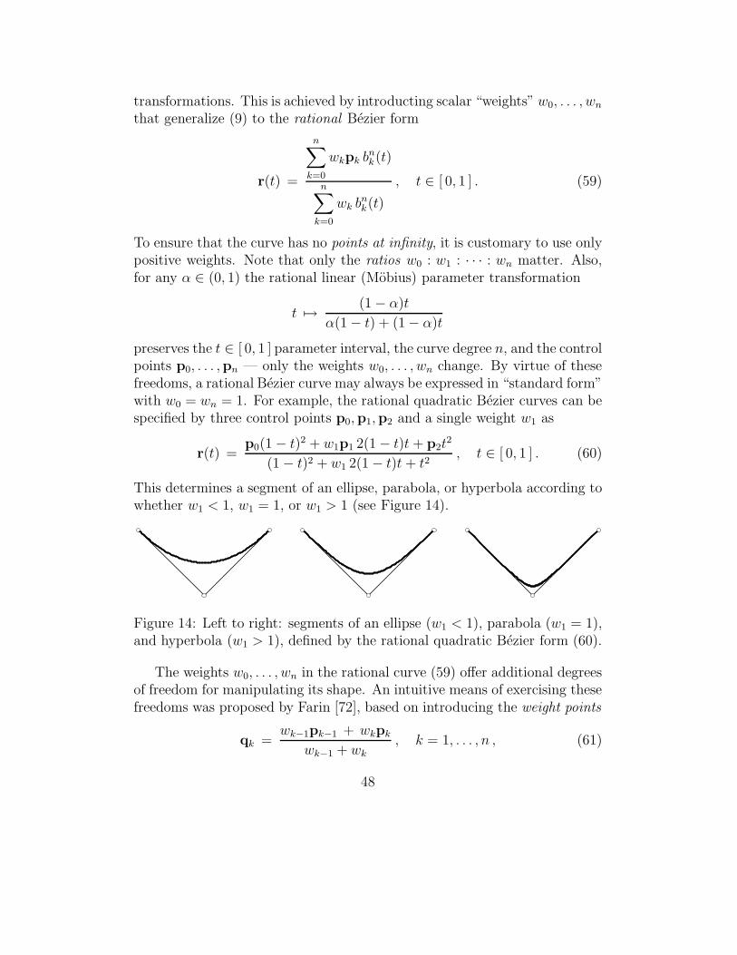
transformations. This is achieved by introducting scalar “weights” w0, . . . , wn
that generalize (9) to the rational Bezier form
r(t) =
n∑
k=0
wkpk bnk(t)
n∑
k=0
wk bnk(t)
, t ∈ [ 0, 1 ] . (59)
To ensure that the curve has no points at infinity, it is customary to use onlypositive weights. Note that only the ratios w0 : w1 : · · · : wn matter. Also,for any α ∈ (0, 1) the rational linear (Mobius) parameter transformation
t 7→ (1 − α)t
α(1 − t) + (1 − α)t
preserves the t ∈ [ 0, 1 ] parameter interval, the curve degree n, and the controlpoints p0, . . . ,pn — only the weights w0, . . . , wn change. By virtue of thesefreedoms, a rational Bezier curve may always be expressed in “standard form”with w0 = wn = 1. For example, the rational quadratic Bezier curves can bespecified by three control points p0,p1,p2 and a single weight w1 as
r(t) =p0(1 − t)2 + w1p1 2(1 − t)t+ p2t
2
(1 − t)2 + w1 2(1 − t)t+ t2, t ∈ [ 0, 1 ] . (60)
This determines a segment of an ellipse, parabola, or hyperbola according towhether w1 < 1, w1 = 1, or w1 > 1 (see Figure 14).
Figure 14: Left to right: segments of an ellipse (w1 < 1), parabola (w1 = 1),and hyperbola (w1 > 1), defined by the rational quadratic Bezier form (60).
The weights w0, . . . , wn in the rational curve (59) offer additional degreesof freedom for manipulating its shape. An intuitive means of exercising thesefreedoms was proposed by Farin [72], based on introducing the weight points
qk =wk−1pk−1 + wkpk
wk−1 + wk, k = 1, . . . , n , (61)
48
on each control polygon leg. The location of qk between pk−1 and pk uniquelyfixes the ratio wk−1 : wk so the n points (61), also called Farin points, specifythe ratios w0 : w1 : · · · : wn. Hence, the curve shape may be manipulated by“sliding” the weight points along the control–polygon legs.
If the rational curve (59) is planar, with control points pk = (xk, yk) fork = 0, . . . , n, its homogeneous coordinates are specified by the polynomials
W (t) =n∑
k=0
wk bnk(t) , X(t) =
n∑
k=0
wkxk bnk(t) , Y (t) =
n∑
k=0
wkyk bnk(t) .
The rational planar curve r(t) may be regarded as the image of a polynomialspace curve R(t) = (W (t), X(t), Y (t)) through a central projection from theorigin (W,X, Y ) = (0, 0, 0) onto the plane W = 1. A 3 × 3 matrix acting onthe homogeneous coordinate polynomials defines a projective transformation
of the curve. These ideas are also readily extended to rational space curves.For a more detailed account of the algorithms and properties associated
with rational Bezier curves, see the paper [69] by Farin. In certain contexts— e.g., the construction of planar Pythagorean–hodograph curves [77, 79] —it is advantageous to interpret planar curves as complex–valued functions ofa real parameter t, i.e., points (x, y) in the plane are identified with complexvalues x + i y, and the rational Bezier curve (59) then has complex controlpoints pk = xk + iyk. Sanchez–Reyes [171] describes a generalization of (59)to the case where the numerator and denominator are both complex–valuedpolynomials. The standard algorithms for rational Bezier curves carry over tosuch forms, which offer compact representations of circular arcs (by rationallinear complex functions), and higher–order curves such as epitrochoids andhypotrochoids. See also Ait–Haddou et al. [3] for some interesting relationsbetween complex polynomials and the geometry of planar polygons.
8.2 Triangular surface patches
The multivariate extension of the Bernstein basis (1) is important for manyapplications. The “tensor–product” scheme, in which the multivariate basisfunctions are simply defined as products of univariate basis functions in eachvariable, is an obvious approach. For example, a tensor–product surface maybe defined over the parameter domain (s, t) ∈ [ 0, 1 ] × [ 0, 1 ] by an array of
49
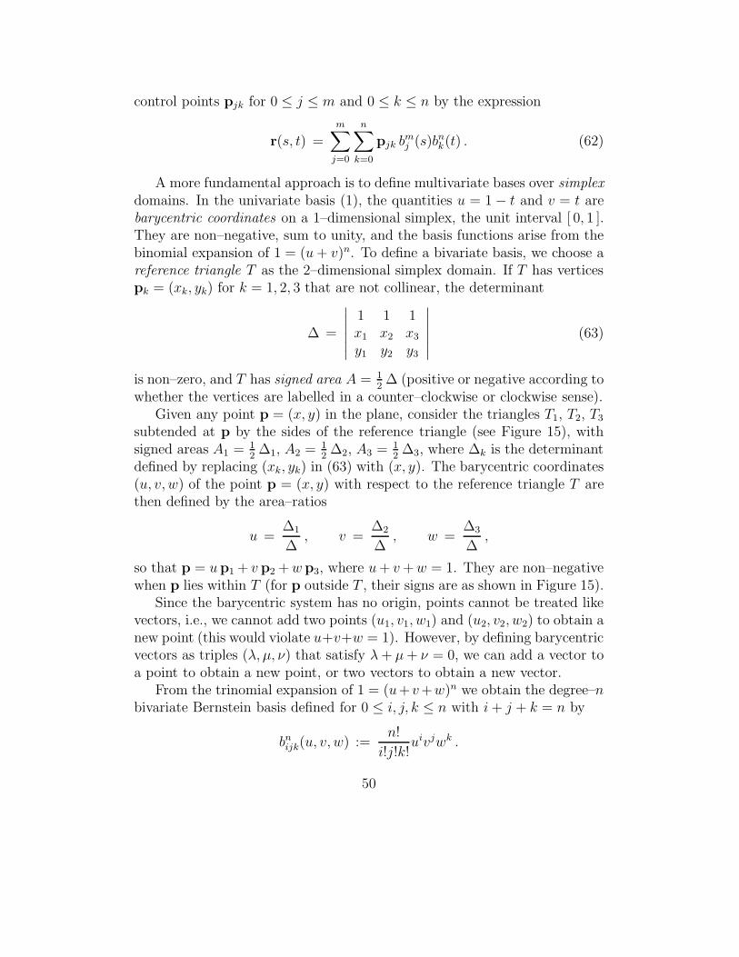
control points pjk for 0 ≤ j ≤ m and 0 ≤ k ≤ n by the expression
r(s, t) =
m∑
j=0
n∑
k=0
pjk bmj (s)bnk(t) . (62)
A more fundamental approach is to define multivariate bases over simplex
domains. In the univariate basis (1), the quantities u = 1 − t and v = t arebarycentric coordinates on a 1–dimensional simplex, the unit interval [ 0, 1 ].They are non–negative, sum to unity, and the basis functions arise from thebinomial expansion of 1 = (u+ v)n. To define a bivariate basis, we choose areference triangle T as the 2–dimensional simplex domain. If T has verticespk = (xk, yk) for k = 1, 2, 3 that are not collinear, the determinant
∆ =
∣∣∣∣∣∣
1 1 1x1 x2 x3
y1 y2 y3
∣∣∣∣∣∣
(63)
is non–zero, and T has signed area A = 12∆ (positive or negative according to
whether the vertices are labelled in a counter–clockwise or clockwise sense).Given any point p = (x, y) in the plane, consider the triangles T1, T2, T3
subtended at p by the sides of the reference triangle (see Figure 15), withsigned areas A1 = 1
2∆1, A2 = 1
2∆2, A3 = 1
2∆3, where ∆k is the determinant
defined by replacing (xk, yk) in (63) with (x, y). The barycentric coordinates(u, v, w) of the point p = (x, y) with respect to the reference triangle T arethen defined by the area–ratios
u =∆1
∆, v =
∆2
∆, w =
∆3
∆,
so that p = up1 + v p2 +w p3, where u+ v+w = 1. They are non–negativewhen p lies within T (for p outside T , their signs are as shown in Figure 15).
Since the barycentric system has no origin, points cannot be treated likevectors, i.e., we cannot add two points (u1, v1, w1) and (u2, v2, w2) to obtain anew point (this would violate u+v+w = 1). However, by defining barycentricvectors as triples (λ, µ, ν) that satisfy λ+ µ+ ν = 0, we can add a vector toa point to obtain a new point, or two vectors to obtain a new vector.
From the trinomial expansion of 1 = (u+v+w)n we obtain the degree–nbivariate Bernstein basis defined for 0 ≤ i, j, k ≤ n with i+ j + k = n by
bnijk(u, v, w) :=n!
i!j!k!uivjwk .
50
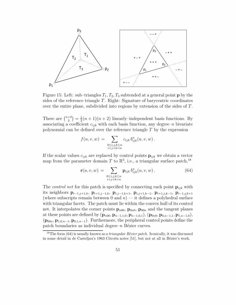
T3
T1T2
p1
p2
p3
p1
p2
p3
+ + +
– – +
– + +
– + –
+ + –
+ – –
+ – +
Figure 15: Left: sub–triangles T1, T2, T3 subtended at a general point p by thesides of the reference triangle T . Right: Signature of barycentric coordinatesover the entire plane, subdivided into regions by extension of the sides of T .
There are(
n+22
)= 1
2(n+ 1)(n+ 2) linearly–independent basis functions. By
associating a coefficient cijk with each basis function, any degree–n bivariatepolynomial can be defined over the reference triangle T by the expression
f(u, v, w) =∑
0≤i,j,k≤ni+j+k=n
cijk bnijk(u, v, w) .
If the scalar values cijk are replaced by control points pijk we obtain a vectormap from the parameter domain T to R3, i.e., a triangular surface patch,18
r(u, v, w) =∑
0≤i,j,k≤ni+j+k=n
pijk bnijk(u, v, w) . (64)
The control net for this patch is specified by connecting each point pijk withits neighbors pi−1,j+1,k, pi+1,j−1,k, pi,j−1,k+1, pi,j+1,k−1, pi+1,j,k−1, pi−1,j,k+1
(where subscripts remain between 0 and n) — it defines a polyhedral surfacewith triangular facets. The patch must lie within the convex hull of its controlnet. It interpolates the corner points pn00, p0n0, p00n and the tangent planesat these points are defined by (pn00,pn−1,1,0,pn−1,0,1), (p0n0,p0,n−1,1,p1,n−1,0),(p00n,p1,0,n−1,p0,1,n−1). Furthermore, the peripheral control points define thepatch boundaries as individual degree–n Bezier curves.
18The form (64) is usually known as a triangular Bezier patch. Ironically, it was discussedin some detail in de Casteljau’s 1963 Citroen notes [51], but not at all in Bezier’s work.
51
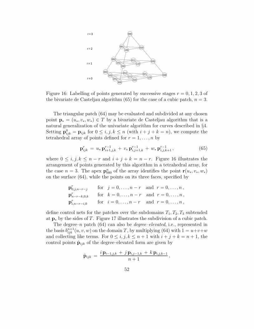
003 012 021 030102 111 120201 210300
002 011 020101 110200
001 010100
000
r = 0
r = 1
r = 2
r = 3
Figure 16: Labelling of points generated by successive stages r = 0, 1, 2, 3 ofthe bivariate de Casteljau algorithm (65) for the case of a cubic patch, n = 3.
The triangular patch (64) may be evaluated and subdivided at any chosenpoint p∗ = (u∗, v∗, w∗) ∈ T by a bivariate de Casteljau algorithm that is anatural generalization of the univariate algorithm for curves described in §4.Setting p0
ijk = pijk for 0 ≤ i, j, k ≤ n (with i + j + k = n), we compute thetetrahedral array of points defined for r = 1, . . . , n by
prijk = u∗ pr−1
i+1,j,k + v∗ pr−1i,j+1,k + w∗ pr−1
i,j,k+1 , (65)
where 0 ≤ i, j, k ≤ n − r and i + j + k = n − r. Figure 16 illustrates thearrangement of points generated by this algorithm in a tetrahedral array, forthe case n = 3. The apex pn
000 of the array identifies the point r(u∗, v∗, w∗)on the surface (64), while the points on its three faces, specified by
pr0,j,n−r−j for j = 0, . . . , n− r and r = 0, . . . , n ,
prn−r−k,0,k for k = 0, . . . , n− r and r = 0, . . . , n ,
pri,n−r−i,0 for i = 0, . . . , n− r and r = 0, . . . , n ,
define control nets for the patches over the subdomains T1, T2, T3 subtendedat p∗ by the sides of T . Figure 17 illustrates the subdivision of a cubic patch.
The degree–n patch (64) can also be degree–elevated, i.e., represented inthe basis bn+1
ijk (u, v, w) on the domain T , by multiplying (64) with 1 = u+v+wand collecting like terms. For 0 ≤ i, j, k ≤ n+ 1 with i+ j + k = n + 1, thecontrol points pijk of the degree–elevated form are given by
pijk =ipi−1,j,k + j pi,j−1,k + k pi,j,k−1
n + 1,
52
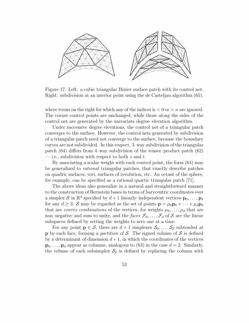
Figure 17: Left: a cubic triangular Bezier surface patch with its control net.Right: subdivision at an interior point using the de Casteljau algorithm (65).
where terms on the right for which any of the indices is< 0 or> n are ignored.The corner control points are unchanged, while those along the sides of thecontrol net are generated by the univariate degree–elevation algorithm.
Under successive degree elevations, the control net of a triangular patchconverges to the surface. However, the control nets generated by subdivisionof a triangular patch need not converge to the surface, because the boundarycurves are not subdivided. In this respect, 3–way subdivision of the triangularpatch (64) differs from 4–way subdivision of the tensor–product patch (62)— i.e., subdivision with respect to both s and t.
By associating a scalar weight with each control point, the form (64) maybe generalized to rational triangular patches, that exactly describe patcheson quadric surfaces, tori, surfaces of revolution, etc. An octant of the sphere,for example, can be specified as a rational quartic triangular patch [71].
The above ideas also generalize in a natural and straightforward mannerto the construction of Bernstein bases in terms of barycentric coordinates overa simplex S in Rd specified by d+ 1 linearly–independent vertices p0, . . . ,pd
for any d ≥ 3. S may be regarded as the set of points p = µ0p0 + · · ·+ µdpd
that are convex combinations of the vertices, for weights µ0, . . . , µd that arenon–negative and sum to unity, and the faces F0, . . . ,Fd of S are the linearsubspaces defined by setting the weights to zero one at a time.
For any point p ∈ S, there are d + 1 simplexes S0, . . . ,Sd subtended atp by each face, forming a partition of S. The signed volume of S is definedby a determinant of dimension d+1, in which the coordinates of the verticesp0, . . . ,pd appear as columns, analogous to (63) in the case d = 2. Similarly,the volume of each subsimplex Sk is defined by replacing the column with
53
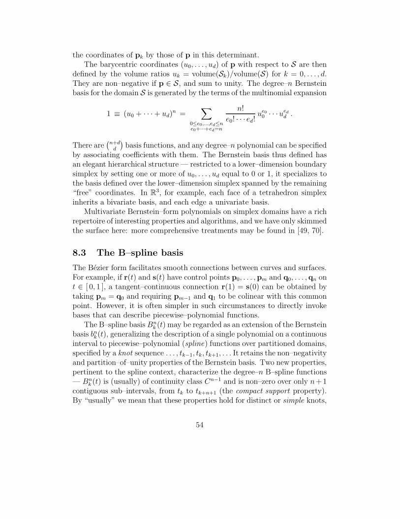
the coordinates of pk by those of p in this determinant.The barycentric coordinates (u0, . . . , ud) of p with respect to S are then
defined by the volume ratios uk = volume(Sk)/volume(S) for k = 0, . . . , d.They are non–negative if p ∈ S, and sum to unity. The degree–n Bernsteinbasis for the domain S is generated by the terms of the multinomial expansion
1 ≡ (u0 + · · ·+ ud)n =
∑
0≤e0,...,ed≤ne0+···+ed=n
n!
e0! · · · ed!ue0
0 · · ·ued
d .
There are(
n+dd
)basis functions, and any degree–n polynomial can be specified
by associating coefficients with them. The Bernstein basis thus defined hasan elegant hierarchical structure — restricted to a lower–dimension boundarysimplex by setting one or more of u0, . . . , ud equal to 0 or 1, it specializes tothe basis defined over the lower–dimension simplex spanned by the remaining“free” coordinates. In R3, for example, each face of a tetrahedron simplexinherits a bivariate basis, and each edge a univariate basis.
Multivariate Bernstein–form polynomials on simplex domains have a richrepertoire of interesting properties and algorithms, and we have only skimmedthe surface here: more comprehensive treatments may be found in [49, 70].
8.3 The B–spline basis
The Bezier form facilitates smooth connections between curves and surfaces.For example, if r(t) and s(t) have control points p0, . . . ,pm and q0, . . . ,qn ont ∈ [ 0, 1 ], a tangent–continuous connection r(1) = s(0) can be obtained bytaking pm = q0 and requiring pm−1 and q1 to be colinear with this commonpoint. However, it is often simpler in such circumstances to directly invokebases that can describe piecewise–polynomial functions.
The B–spline basis Bnk (t) may be regarded as an extension of the Bernstein
basis bnk(t), generalizing the description of a single polynomial on a continuousinterval to piecewise–polynomial (spline) functions over partitioned domains,specified by a knot sequence . . . , tk−1, tk, tk+1, . . . It retains the non–negativityand partition–of–unity properties of the Bernstein basis. Two new properties,pertinent to the spline context, characterize the degree–n B–spline functions— Bn
k (t) is (usually) of continuity class Cn−1 and is non–zero over only n+1contiguous sub–intervals, from tk to tk+n+1 (the compact support property).By “usually” we mean that these properties hold for distinct or simple knots,
54
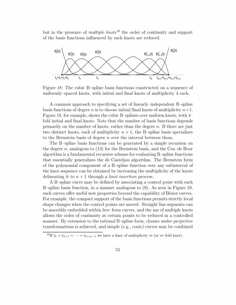
but in the presence of multiple knots19 the order of continuity and supportof the basis functions influenced by such knots are reduced.
t0=t1=t2=t3 t4 t5 tN tN+1=tN+2=tN+3=tN+4
B30(t)
B31(t) B3
2(t)B3
3(t) B3N–2(t) B3
N–1(t)B3
N(t)
Figure 18: The cubic B–spline basis functions constructed on a sequence ofuniformly–spaced knots, with initial and final knots of multiplicity 4 each.
A common approach to specifying a set of linearly–independent B–splinebasis functions of degree n is to choose initial/final knots of multiplicity n+1.Figure 18, for example, shows the cubic B–splines over uniform knots, with 4–fold initial and final knots. Note that the number of basis functions dependsprimarily on the number of knots, rather than the degree n. If there are justtwo distinct knots, each of multiplicity n + 1, the B–spline basis specializesto the Bernstein basis of degree n over the interval between them.
The B–spline basis functions can be generated by a simple recursion onthe degree n, analogous to (13) for the Bernstein basis, and the Cox–de Booralgorithm is a fundamental recursive scheme for evaluating B–spline functionsthat essentially generalizes the de Casteljau algorithm. The Bernstein formof the polynomial component of a B–spline function over any subinterval ofthe knot sequence can be obtained by increasing the multiplicity of the knotsdelineating it to n + 1 through a knot insertion process.
A B–spline curve may be defined by associating a control point with eachB–spline basis function, in a manner analogous to (9). As seen in Figure 19,such curves offer useful new properties beyond the capability of Bezier curves.For example, the compact support of the basis functions permits strictly localshape changes when the control points are moved. Straight line segments canbe smoothly embedded within free–form curves, and the use of multiple knotsallows the order of continuity at certain points to be reduced in a controlledmanner. By extension to the rational B–spline form, closure under projectivetransformations is achieved, and simple (e.g., conic) curves may be combined
19If tk = tk+1 = · · · = tk+m−1 we have a knot of multiplicity m (or m–fold knot).
55
Figure 19: Left: local modification of a cubic B–spline curve by displacementof a single control point — note that C2 connections between the modifiedand unmodified segments are maintained. Right: A line segment embeddedin a C2 cubic B–spline curve (four consecutive control points are collinear).
with free–form segments in an integrated representation format. A completeaccount of the B–spline form is beyond the scope of this survey — the intenthere is simply to highlight its intimate connections to the Bernstein basis.Complete details may be found in standard texts, e.g., [47, 74, 173].
8.4 Generalized barycentric coordinates
Although triangular and rectangular surface patches are predominant in mostdesign applications, the need for patches with N ≥ 5 sides often arises, anda number of schemes to permit their construction subject to given boundaryconditions have been formulated [38, 107, 115, 126, 134, 209]. Such N–sidedpatches must typically interpolate given boundary curves and cross–tangentdata along them, to ensure G1 continuity with adjacent patches.
Noteworthy among these formulations are the S–patches [134] of Loop andDeRose, and the toric surface patches introduced by Krasauskas [126]. Theformer defines an N–sided patch by embedding an N–sided domain polygonP in a simplex S of dimension N − 1, such that the sides of P coincide withedges of S. When a vector–valued Bernstein–form polynomial is constructedover the simplex S, its restriction to the polygon P yields an N–sided surfacepatch. The latter constructs rational N–sided patches over polygon domainswith vertices that have integer coordinates. Both schemes subsume triangularand tensor–product Bezier surface patches as special cases.
The study of N–sided patches has also prompted interest in extending the
56
definition of barycentric coordinates from triangular or simplex domains tomore general polygons or polytopes. In extending from simplexes to generalconvex polytopes, one must incorporate certain properties of the barycentriccoordinates [210] — if λ1, . . . , λN are the barycentric coordinates of a point p
with respect to a polytope P defined by vertices v1, . . . ,vN in Rd we require:
(1) non–negativity : λ1, . . . , λN ≥ 0 for all p ∈ P;
(2) linear precision: λ1f(v1)+· · ·+λNf(vN) ≡ f(p) for any linear functionf(p). Choosing f(p) = 1, this implies the partition of unity property,i.e., λ1 + · · · + λN = 1 for all p.
(3) minimal degree: λ1, . . . , λN are the “simplest” functions of the locationof p that satisfy (1) and (2).
For a simplex, condition (3) is achieved with a linear dependence of λ1, . . . , λN
on the location of p. For a more general polytope, λ1, . . . , λN have a rational
dependence on the location of p. The first construction of such a system wasperformed by Wachspress [207] in the context of constructing a finite elementbasis for convex polygons — see also [45, 208]. For a convex polygon with msides, the barycentric coordinates are rational functions with numerators ofdegree m− 2, and a denominator of degree m− 3 that defines the adjoint ofthe polygon, i.e., the algebraic curve that passes through the pairwise pointsof intersection of the linear extensions to the polygon sides (other than thepolygon vertices). Meyer et al. [143] showed that the Wachspress coordinatescan be expressed (see Figure 20) as
λk :=wk
w1 + · · ·+ wN, wk :=
area(vk−1,vk,vk+1)
area(vk−1,vk,p) area(p,vk,vk+1),
where vertex indices are interpreted cyclically, and area( ) is the signed areaof the triangle determined by the indicated points. Warren [210] subsequentlygeneralized the Wachspress scheme to convex polytopes of any dimension; anextension to the case of smooth convex sets may also be found in [211].
A different approach based on the mean value theorem was introduced byFloater [87]. These “mean value coordinates” are defined by
λk :=wk
w1 + · · ·+ wN, wk :=
tan 12αk−1 + tan 1
2αk
rk,
57
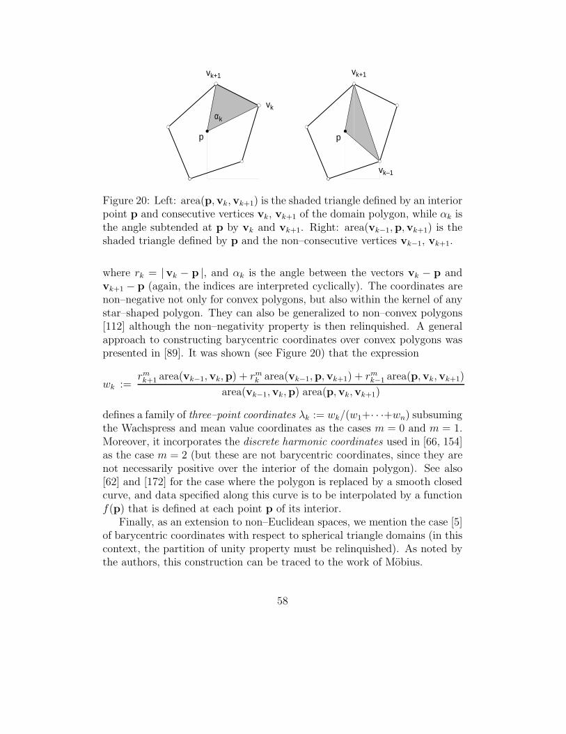
p
vk
vk+1
αk
p
vk–1
vk+1
Figure 20: Left: area(p,vk,vk+1) is the shaded triangle defined by an interiorpoint p and consecutive vertices vk, vk+1 of the domain polygon, while αk isthe angle subtended at p by vk and vk+1. Right: area(vk−1,p,vk+1) is theshaded triangle defined by p and the non–consecutive vertices vk−1, vk+1.
where rk = |vk − p |, and αk is the angle between the vectors vk − p andvk+1 − p (again, the indices are interpreted cyclically). The coordinates arenon–negative not only for convex polygons, but also within the kernel of anystar–shaped polygon. They can also be generalized to non–convex polygons[112] although the non–negativity property is then relinquished. A generalapproach to constructing barycentric coordinates over convex polygons waspresented in [89]. It was shown (see Figure 20) that the expression
wk :=rmk+1 area(vk−1,vk,p) + rm
k area(vk−1,p,vk+1) + rmk−1 area(p,vk,vk+1)
area(vk−1,vk,p) area(p,vk,vk+1)
defines a family of three–point coordinates λk := wk/(w1+· · ·+wn) subsumingthe Wachspress and mean value coordinates as the cases m = 0 and m = 1.Moreover, it incorporates the discrete harmonic coordinates used in [66, 154]as the case m = 2 (but these are not barycentric coordinates, since they arenot necessarily positive over the interior of the domain polygon). See also[62] and [172] for the case where the polygon is replaced by a smooth closedcurve, and data specified along this curve is to be interpolated by a functionf(p) that is defined at each point p of its interior.
Finally, as an extension to non–Euclidean spaces, we mention the case [5]of barycentric coordinates with respect to spherical triangle domains (in thiscontext, the partition of unity property must be relinquished). As noted bythe authors, this construction can be traced to the work of Mobius.
58
9 Further applications
As the Bernstein form has matured and proved its worth as a core paradigmof CAGD, interest in taking advantage of the useful properties and algorithmsdeveloped in that context for other computational disciplines has exhibitedincreasing momentum in recent years. Some applications that have benefitedsignificantly from this trend are briefly discussed below.
9.1 Equations and inequalities
The ability to compute the real roots of a polynomial or solutions of a systemof algebraic equations, to determine the extrema of (or estimate bounds on)polynomials in one or several variables over finite domains, and to optimizepolynomial functions under given constraints, are key requirements in manyscientific/engineering problems. The subdivision, convex hull, and variation–diminishing features of the Bernstein form are very useful in such contexts.
The basic problem of isolating and approximating the roots of a univariateBernstein–form polynomial p(t) on the interval [ 0, 1 ] was addressed by Laneand Riesenfeld [131]. Their algorithm employs recursive subdivision until theBernstein coefficients for each subinterval exhibit either no sign changes orjust one sign change. By the variation–diminishing property, subintervals inthe former category contain no roots, and those in the latter category containprecisely one root.20 Once the real roots are isolated within sufficiently smallsubintervals, rapidly–convergent approximation methods can be invoked toapproximate them to any desired accuracy. For example, simple conditionsfor guaranteed convergence of the Newton–Raphson method
tk+1 = tk − p(tk)
p′(tk), k = 1, 2, . . . (66)
can be easily expressed in terms of the Bernstein coefficients c0, . . . , cn of p(t)for any subinterval [ a, b ] on which they have exactly one sign change (withc0cn < 0). Namely, the iteration (66) will converge to the unique real root ofp(t) on the interval (a, b) from any start point within it, if we have
S(∆c0, . . . ,∆cn−1) = 0 , (67)
20For subintervals containing multiple roots, the condition of zero or one coefficient signchanges will not be met under repeated subdivision. To accommodate multiple roots, thealgorithm must be modified to consider also roots of the derivatives of p(t) — see [224].
59
S(∆2c0, . . . ,∆2cn−2) = 0 , (68)
|c0| ≤ n |∆c0| and |cn| ≤ n |∆cn−1| , (69)
where ∆ck = ck+1 − ck, ∆2ck = ∆ck+1 − ∆ck = ck+2 − 2ck+1 + ck, and S( )indicates the number of sign changes in the ordered sequence of its arguments.Conditions (67) and (68) ensure that p(t) has non–vanishing first and secondderivatives for t ∈ (a, b). The former implies that p(t) is monotone over (a, b)and therefore has only one root in that interval. The latter implies that thegraph of p(t) is convex or concave over (a, b). Finally, condition (69) ensuresthat the tangent lines to p(t) at t = a and t = b cross the t–axis within theinterval (a, b). A proof of this result may be found in [108, p. 79].
The above scheme may be modified and improved in a number of ways toexploit further properties of the Bernstein form — the PhD thesis of Spencer[191], for example, describes a number of interesting variants. The numericalstability of the Bernstein form (see Section 6) is invaluable in the context ofroot–solvers based on floating–point arithmetic operations.
The extension to systems of polynomial equations in several variables isa non–trivial problem, since the variation–diminishing property of univariatepolynomials has no straightforward multivariate generalization. Nonetheless,several methods exploiting the subdivision and convex hull properties havebeen developed for tensor–product multivariate Bernstein–form polynomials[95, 147, 148, 181]. Lack of space precludes a thorough description of thesemethods here: complete details may be found in the cited references.
Closely–related problems are concerned with estimations of the range ofmultivariate polynomials over given subdomains, in the context of relaxationsteps employed in the “branch–and–bound” approach to solving optimizationproblems [91, 94, 150, 166, 190]. The subdivision and convex hull propertiesof the Bernstein form again play a key role, along with simple monotonicityand convexity tests over subdomains. Most of this work has addressed onlytensor–product polynomials defined over rectangular domains in R
n, but theextension to barycentric forms over simplex domains is straightforward.
9.2 Finite element analysis
Since the geometric models created within CAD systems serve as the point ofdeparture for various physical analyses using the finite element method, onemight expect close coordination in the evolution of these fields. For manydecades, however, they have evolved in a largely independent manner.
60
The “isogeometric analysis” paradigm seeks to remedy this disconnectby using NURBS (non–uniform rational B–splines), a commonly–used CADgeometry format, as shape functions in the analysis, bypassing much of thecostly and error–prone meshing requirements of traditional FEM approaches[117]. Insofar as B–spline forms generalize the Bernstein form to partitioneddomains, the method may be considered to fall within the scope of this survey.The key challenge lies in accommodating “trimmed” surface patches — whichare invariably present in complex geometric models, but incompatible withstandard tensor–product NURBS domains. We focus here on recent methodsthat directly exploit the Bernstein form in finite element analysis.
Bogdanovich [23, 24, 25, 26] describes the use of tensor–product trivariateBernstein basis functions to specify three–dimensional displacement fields inhexahedral finite elements, for the analysis of stresses in laminated compositestructures with anisotropic material properties. In the context of composites,different continuity properties of the element “shape functions” are desired indirections parallel and perpendicular to interfaces between distinct materials.The Bernstein form facilitates the enforcement of appropriate displacementand stress continuity conditions, and closed–form computation — rather thannumerical quadrature — for various integrals that determine the elements ofmatrices required in the stress analysis. The author argues that the Bernsteinbasis functions “a rarity in structural analysis, deserve more attention” [23].
Schumaker [174] describes the use of bivariate spline functions defined ontriangulations, in which the Bernstein polynomial form is used to specify thevariation over each triangular subdomain, to solve boundary value problemsfor elliptic partial differential equations: see also [129]. Bernstein–form finiteelement algorithms for simplicial domains have also recently been studied byKirby [121, 122] with emphasis on efficient algorithms for computing massand stiffness matrices for high–order polynomials on simplex domains, and onformulation of matrix–free algorithms. A closely–related paper by Ainsworthet al. [2] shows that finite element algorithms for high–order Bernstein–formpolynomials over simplex domains, based upon the Duffy transformation [61],can achieve computational complexity comparable to that for tensor–productformulations. It is noteworthy [2] that, in 2011, use of the Bernstein form “hasattracted virtually no attention . . . among the finite element community.” Anexception is the paper by Scott et al. [176] on using T–splines (which providemore topological flexibility than tensor–product B–splines) for isogeometricanalysis, and extracting Bernstein–form elements from T–spline models.
A generalization of the simplicial Bernstein basis described by Arnold et
61
al. [7] is concerned with the characterization and geometric decomposition ofspaces of finite element differential forms, extending classical finite elementvector field spaces in R2 and R3 to higher–order forms and space dimensions.
The barycentric coordinates on simplex domains that are used to defineBernstein bases also admit useful generalizations. For example, given a set ofpoints p1, . . . ,pn in the plane, their Voronoi diagram or Dirichlet tessellation
[159] comprises a set of contiguous polygonal tiles T1, . . . , Tn such that pk ∈Tk and every point of Tk is closer to pk than to all the other points pj forj 6= k. When a new point p is introduced,21 a new tile T will be associatedwith it in the updated tessellation, overlapping certain tiles Tk1
, . . . , Tkmof
the original tessellation. The location of p can be specified in terms of itsneighbor points pk1
, . . . ,pkmin the form
p =m∑
j=1
uj pkj,
where uj is the fractional area of T that overlaps Tkj. The Sibson coordinates
[182] u1, . . . , um of p are non–negative and form a partition of unity — i.e.,u1, . . . , um ≥ 0 and u1+ · · ·+um = 1. Furthermore, when there are just threeneighbor points (m = 3), these Sibson coordinates specialize to barycentriccoordinates over the triangle defined by those points.
The Sibson (or natural neighbor) coordinates are unique, and continuouswith respect to the location of p. Furthermore, they can be generalized fromR2 to Rn for n ≥ 3, since the Dirichlet tessellation is defined in any numberof Euclidean dimensions. Sibson [183] defined an interpolant to data valuesf1, . . . , fn associated with the data sites p1, . . . ,pn by the expression
f(u1, . . . , um) =m∑
j=1
fjuj . (70)
Farin [73] showed that Sibson’s interpolant exhibits C1 continuity and haslinear precision (see Section 8.4), and interpreted (70) as the projection of alinear Bernstein–form polynomial, defined on a simplex of dimension m− 1.Using the Bernstein form, he also proposed a generalized interpolant withquadratic precision (completeness) — i.e., when f1, . . . , fn are sampled froma quadratic function, it exactly recovers that function.
21The new point p must lie in the convex hull of the given points p1, . . . ,pn.
62
In the finite element context, the generalized Sibson interpolant has beenadopted [30, 199, 200] as the basis for an approach called the natural element
method, which may be considered “meshfree” or “meshless” since it does notrequire any element connectivity information. The methods for generalizingbarycentric coordinates from simplex domains to general polygons/polytopesdiscussed in Section 8.4 have also attracted interest within the finite elementresearch community. As noted above, these ideas originated with the rationalfinite element basis of Wachspress [207]. More recent results can be found in[45, 138, 139, 198, 201]. An interesting new method, the “maximum entropy”approach, interprets the construction of barycentric coordinates over generalpolygons/polytopes as a least–biased solution of an underdetermined systemof linear equations [113, 197]. Closed–form expressions for the coordinatesare no longer available in this context, but they can be efficiently computedthrough a constrained optimization problem.
9.3 Robust control of dynamic systems
A key consideration in designing controllers for linear dynamic systems is theselection of controller “gains” that are consistent with desired performanceand stability of the controller, i.e., for any bounded input, the system outputshould remain bounded. The stability of a linear system can be characterizedby the complex–plane distribution of the roots of its characteristic polynomial
[60] — for analog systems, the roots must all lie to the left of the imaginaryaxis (Hurwitz condition); for digital systems, the roots must all lie within theunit disk centered on the origin of the complex plane (Schur condition).
The problem of robust control is concerned with systems whose physicalparameters are not precisely known, but may vary within prescribed ranges.Thus, instead of a unique characteristic polynomial, the stability analysis ofsuch systems incurs parameter–dependent characteristic polynomials. To berobustly stable, each instance of the system — corresponding to each possiblecombination of the parameter values — must be stable [1, 8].
To guarantee certain performance criteria beyond nominal stability, it isoften desirable to restrict the characteristic polynomial roots to some subsetΓ of the left half–plane, or unit disk — the system is then said to be Γ–stable.Suppose the characteristic polynomial has the form
p(t) =n∑
k=0
ak(q1, . . . , qm) tk (71)
63
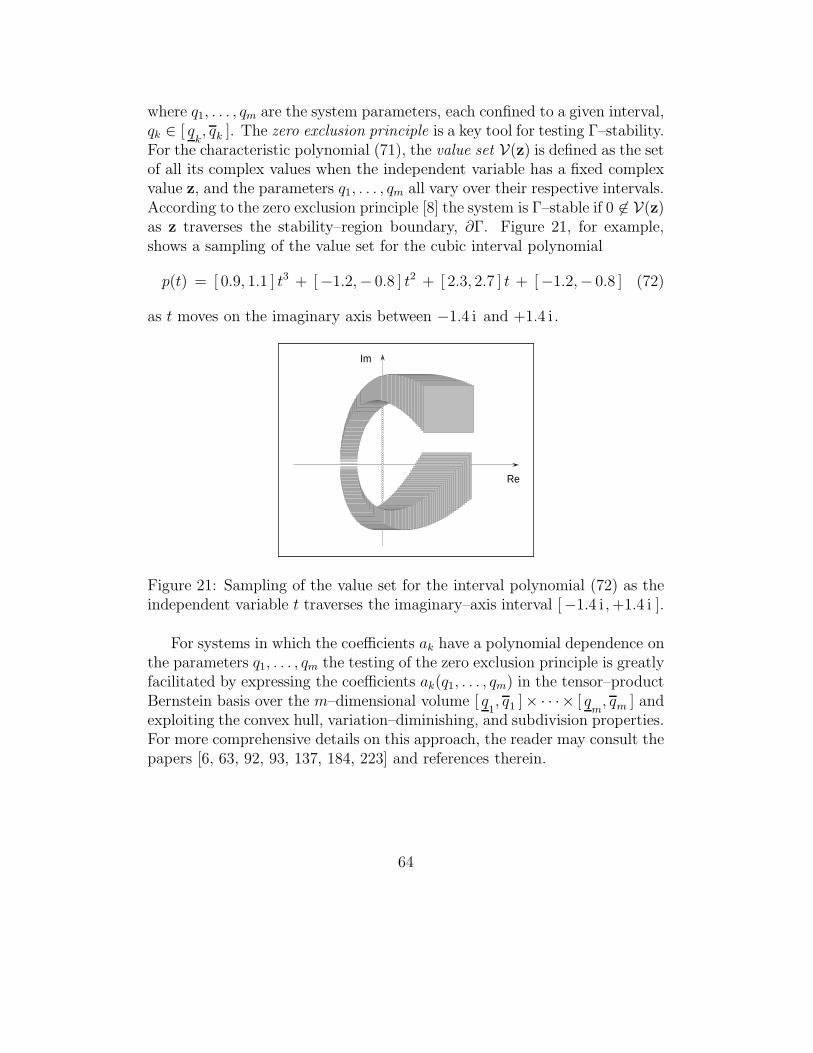
where q1, . . . , qm are the system parameters, each confined to a given interval,qk ∈ [ q
k, qk ]. The zero exclusion principle is a key tool for testing Γ–stability.
For the characteristic polynomial (71), the value set V(z) is defined as the setof all its complex values when the independent variable has a fixed complexvalue z, and the parameters q1, . . . , qm all vary over their respective intervals.According to the zero exclusion principle [8] the system is Γ–stable if 0 6∈ V(z)as z traverses the stability–region boundary, ∂Γ. Figure 21, for example,shows a sampling of the value set for the cubic interval polynomial
p(t) = [ 0.9, 1.1 ] t3 + [−1.2,− 0.8 ] t2 + [ 2.3, 2.7 ] t + [−1.2,− 0.8 ] (72)
as t moves on the imaginary axis between −1.4 i and +1.4 i .
Re
Im
Figure 21: Sampling of the value set for the interval polynomial (72) as theindependent variable t traverses the imaginary–axis interval [−1.4 i ,+1.4 i ].
For systems in which the coefficients ak have a polynomial dependence onthe parameters q1, . . . , qm the testing of the zero exclusion principle is greatlyfacilitated by expressing the coefficients ak(q1, . . . , qm) in the tensor–productBernstein basis over the m–dimensional volume [ q
1, q1 ]× · · ·× [ q
m, qm ] and
exploiting the convex hull, variation–diminishing, and subdivision properties.For more comprehensive details on this approach, the reader may consult thepapers [6, 63, 92, 93, 137, 184, 223] and references therein.
64
9.4 Other problems
Applications of the Bernstein basis have also elicited interest in many othercomputational problems, a few of which are briefly mentioned here. In [110]the Bernstein basis is employed in modeling inter–molecular potential energysurfaces through the reproducing kernel Hilbert space interpolation method.Algorithms for neurofuzzy networks modelling non–linear dynamical systemshave invoked the bivariate Bernstein basis on triangular domains to representthe system input [111]. Tensor–product Bernstein basis neural networks havealso been used in reconstructing 3D models from measured data and in thecalibration of optical range sensors [123, 124]. Degree elevation of univariateBernstein–form polynomials has been employed in [170] to facilitate designof filter sharpening functions for signal processing applications. Convergentpiecewise–linear approximations obtained from the Bernstein form have beeninvoked [68, 85] in computing time–optimal feedrates along curved paths forCNC machines with prescribed axis acceleration bounds, which amounts toa calculus of variations problem with polynomial point–wise constraints.
10 Closure
This survey has endeavored to describe the historical origins, current status,and diverse applications of the Bernstein polynomial basis, on the centennialanniversary of its introduction. The adoption of the Bernstein representationas a medium for practical computations has been an evolutionary process, inwhich three distinct phases may be clearly discerned.
First, beginning with Bernstein’s 1912 paper, it served as a fundamentaltheoretical tool for analyzing the approximative capability of polynomials onfinite domains. However, the necessity of proceeding to very high degrees toenforce tight error bounds precluded widespread use of Bernstein polynomialapproximations in practical computations. Second, the work of de Casteljauand Bezier in the 1960s revealed that the Bernstein form provides an excellentmedium for the specification/modification of (vector–valued) polynomials onfinite domains, although at first their ideas were not explicitly identified withthe Bernstein basis. The ensuing elaboration of algorithms and properties forthe “Bernstein–Bezier form” in the field of computer aided geometric design
has led to a high degree of maturity and utility for this representation. Third,drawing on the extensive body of methods developed in the CAGD context,
65
the attractive features of the Bernstein form have been increasingly exploitedin other scientific and engineering applications over the past few decades (seeSection 9). It can be expected that a further development and diversificationof this latter phase may continue for many years to come.
The volume of papers concerned with properties, algorithms, applications,and extensions of the Bernstein polynomial representation has grown to vastproportions over the past century. Although it has not been possible to citeevery relevant work herein, it is nevertheless hoped that this survey offers abalanced perspective on the principal research themes and trends, and thushelps encourage further useful applications of the Bernstein form.
Acknowledgements
The idea for this survey originated among discussions between Ron Goldman,Hartmut Prautzsch, and others at a meeting in Schloss Dagstuhl in May 2011.The author is grateful for being given the opportunity to write it. The paperhas been greatly improved by the efforts of the anonymous referees, throughtheir diligent reading of and perceptive comments on an initial draft. Finally,the author acknowledges the kind help of several colleagues (V. S. Bagrova,M. S. Floater, A. Kurnosenko, J–J. Martinez, T. W. Sederberg, Y. Simsek,N. Sukumar, J. Warren) who provided advice, materials, and suggestions.
References
[1] J. Ackermann (1993), Robust Control: Systems with Uncertain
Physical Parameters, Springer, London.
[2] M. Ainsworth, G. Adriamaro, and O. Davydov (2011),Bernstein–Bezier finite elements of arbitrary order and optimalassembly procedures, SIAM Journal on Scientific Computing 33,3087–3109.
[3] R. Ait–Haddou, W. Herzog, and T. Nomura (2010), Complex Beziercurves and the geometry of polygons, Computer Aided Geometric
Design 27, 525–537.
[4] N. I. Akhiezer (1955), Akademik S. N. Bernshtein i ego raboty po
konstruktivnoy teorii funktsy (The academician S. N. Bernstein
66
and his contributions to constructive function theory), Kharkov— translated into German by R. K. Kovacheva and H. H. Gonskaas Das Akademiemitglied S. N. Bernstein und seine Arbeiten zur
konstruktiven Funktionentheorie, Giessen (2000).
[5] P. Alfeld, M. Neamtu, and L. L. Schumaker (1996), Bernstein–Bezierpolynomials on spheres and sphere–like surfaces, Computer Aided
Geometric Design 13, 333–349.
[6] H. Akyar, T. Buyukkoroglu, and V. Dzhafarov (2010), On stability ofparameterized families of polynomials and matrices, Abstract and
Applied Analysis, Article No. 687951.
[7] D. N. Arnold, R. S. Falk, and R. Winther (2009), Geometricdecompositions and local bases for spaces of finite element differentialforms, Computer Methods in Applied Mechanics and Engineering
198, 1660-1672.
[8] B. R. Barmish (1994), New Tools for Robustness of Linear Systems,Macmillan, New York.
[9] J. Berchtold and A. Bowyer (2000), Robust arithmetic formultivariate Bernstein–form polynomials, Computer Aided Design 32,681–689.
[10] S. N. Bernstein (1912), Demonstration du theoreme de Weierstrassfondee sur le calcul des probabilites, Communications de la Societe
Mathematique de Kharkov 2. Series XIII No. 1, 1–2.
[11] P. Bezier (1966), Definition numerique des courbes et surfaces I,Automatisme XI, 625–632.
[12] P. Bezier (1967), Definition numerique des courbes et surfaces II,Automatisme XII, 17–21.
[13] P. Bezier (1971), Example of an existing system in the motorindustry: the UNISURF system, Proceedings of the Royal Society of
London A 321, 207–218.
[14] P. Bezier (1972), Numerical Control: Mathematics and Applications
(translated by A. R. Forrest and A. F. Pankhurst), Wiley, London.
67

[15] P. Bezier (1974), Mathematical and practical possibilities ofUNISURF, in Computer Aided Geometric Design (R. E. Barnhill andR. F. Riesenfeld, eds.), Academic Press, New York, pp. 127–152.
[16] P. Bezier (1977), Essai de Definition Numerique des Courbes et desSurfaces Experimentales, PhD Thesis, University of Paris VI.
[17] P. Bezier (1986), The Mathematical Basis of the UNISURF CAD
System, Butterworths, London.
[18] P. E. Bezier (1993), The first years of CAD/CAM and the UNISURFCAD system, in Fundamental Developments of Computer–Aided
Geometric Modeling (L. Piegl, ed.), Academic Press, London,pp. 13–26.
[19] D. A. Bini and L. Gemignani (2004), Bernstein–Bezoutian matrices,Theoretical Computer Science 315, 319–333.
[20] D. A. Bini, L. Gemignani, and J. R. Winkler (2005), Structuredmatrix methods for CAGD: An application to computing theresultant of polynomials in the Bernstein basis, Numerical Linear
Algebra with Applications 12, 685–698.
[21] W. Boehm (1988), On de Boor–like algorithms and blossoming,Computer Aided Geometric Design 5, 71–79.
[22] W. Boehm and A. Muller (1999), On de Casteljau’s algorithm,Computer Aided Geometric Design 16, 587–605.
[23] A. E. Bogdanovich (2000), Three–dimensional variational theory oflaminated composite plates and its implementation with Bernsteinbasis functions, Computer Methods in Applied Mechanics and
Engineering 185, 279–304.
[24] A. E. Bogdanovich (2001), Three–dimensional variational analysis ofcomposite structures using Bernstein polynomial approximations,Reports 1 & 2, Mechanics of Composite Materials 37, 525–538 &539–552.
[25] A. E. Bogdanovich, C. M. Pastore, and B. P. Deepak (1995), Acomparison of various 3D approaches for the analysis of laminatedcomposite structures, Composites Engineering 5, 1105–1126.
68
[26] A. E. Bogdanovich and S. P. Yushanov (1999), Progressive failureanalysis of adhesive bonded joints with laminated compositeadherends, Journal of Reinforced Plastics and Composites 18,1689–1707.
[27] W. Bohm (1977), Uber die Konstruktion von B–Spline–Kurven,Computing 18, 161–166.
[28] W. Bohm, G. Farin, and J. Kahmann (1984), A survey of curve andsurface methods in CAGD, Computer Aided Geometric Design 1,1–60.
[29] J. P. Boyd (2008), Exploiting parity in converting to and fromBernstein polynomials and orthogonal polynomials, Applied
Mathematics and Computation 198, 925–929.
[30] J. Braun and M. Sambridge (1995), A numerical method for solvingpartial differential equations on highly irregular evolving grids, Nature
376, 655–660.
[31] G. Brunnett, T. Schreiber, and J. Braun (1996), The geometry ofoptimal degree reduction of Bezier curves, Computer Aided Geometric
Design 13, 773–788.
[32] W. S. Burnside and A. W. Panton (1928), The Theory of Equations,Dover Publications (reprint), New York.
[33] L. Buse and R. Goldman (2008), Division algorithms for Bernsteinpolynomials, Computer Aided Geometric Design 25, 850–865.
[34] G. T. Cargo and O. Shisha (1966), The Bernstein form of apolynomial, Journal of Research of the National Bureau of Standards
— B. Mathematics and Mathematical Physics 70B, 79–81.
[35] J. M. Carnicer and J. M. Pena (1993), Shape preservingrepresentations and optimality of the Bernstein basis, Advances in
Computational Mathematics 1, 173–196.
[36] G. Chang (1984), Bernstein polynomials via the shifting operator,American Mathematical Monthly 91, 634–638.
69
[37] G. Chang and J. Wu (1981), Mathematical foundations of Bezier’stechnique, Computer Aided Design 13, 133–136.
[38] P. Charrot and J. A. Gregory (1984), A pentagonal surface patch forcomputer aided geometric design, Computer Aided Geometric Design
1, 87–94.
[39] E. Cohen and L. L. Schumaker (1985), Rates of convergence ofcontrol polygons, Computer Aided Geometric Design 2, 229–235.
[40] L. Coluccio, A. Eisinberg, and G. Fedele (2008), Gauss–Lobatto toBernstein polynomials transformation, Journal of Computational and
Applied Mathematics 222, 690–700.
[41] M. J. Crowe (1967), A History of Vector Analysis, Dover Publications(reprint), New York.
[42] E. W. Cheney (1966), Introduction to Approximation Theory,McGraw–Hill, New York.
[43] W. Dahmen (1986), Subdivision algorithms converge quadratically,Journal of Computational and Applied Mathematics 16, 145–158.
[44] M. Daniel and J. C. Daubisse (1989), The numerical problem of usingBezier curves and surfaces in the power basis, Computer Aided
Geometric Design 6, 121–128.
[45] G. Dasgupta (2003), Interpolants within convex polygons: Wachspressshape functions, Journal of Aerospace Engineering 16, 1–8.
[46] P. J. Davis (1975), Interpolation and Approximation, DoverPublications (reprint), New York.
[47] C. de Boor (2001), A Practical Guide to Splines (revised edition),Springer, New York.
[48] C. de Boor (1987), Cutting corners always works, Computer Aided
Geometric Design 4, 125–131.
[49] C. de Boor (1987), B–form basics, in G. E. Farin (ed.), Geometric
Modeling: Algorithms and New Trends, SIAM, Philadelphia,pp. 131–148.
70
[50] C. de Boor and K. Hollig (1987), B–splines without divideddifferences, in G. E. Farin (ed.), Geometric Modeling: Algorithms and
New Trends, SIAM, Philadelphia, pp. 21–27.
[51] P. de Casteljau (1963), Courbes et Surfaces a Poles, Societe AnonymeAndre Citroen, Internal Report.
[52] P. de Casteljau (1985), Formes a Poles, Hermes, Paris.
[53] P. de Casteljau (1986), Shape Mathematics and CAD, Kogan–Page,London.
[54] P. de Casteljau (1987), Les Quaternions, Hermes, Paris.
[55] P. de Casteljau (1991), POLynomials, POLar forms, andinterPOLation, in Mathematical Methods in Computer Aided
Geometric Design II (T. Lyche and L. L. Schumaker, eds.), AcademicPress, Boston, pp. 57–68.
[56] P. de Casteljau (1993), Polar forms for curve and surface modelling asused at Citroen, in Fundamental Developments of Computer–Aided
Geometric Modeling (L. Piegl, ed.), Academic Press, London,pp. 1–11.
[57] P. de Faget de Casteljau (1999), De Casteljau’s autobiography: Mytime at Citroen, Computer Aided Geometric Design 16, 583–586.
[58] J. Delgado and J. M. Pena (2009), Optimal conditioning of Bernsteincollocation matrices, SIAM Journal on Matrix Analysis and
Applications 31, 990–996.
[59] T. D. DeRose (1988), Composing Bezier simplexes, ACM
Transactions on Graphics 7, 198–221.
[60] R. C. Dorf and R. H. Bishop (2005), Modern Control Systems, 10thedition, Pearson Prentice Hall, Upper Saddle River, NJ.
[61] M. G. Duffy (1982), Quadrature over a pyramid or cube of integrandswith a singularity at a vertex, SIAM Journal on Numerical Analysis
19, 1260–1262.
71
[62] C. Dyken and M. S. Floater (2009), Transfinite mean valueinterpolation, Computer Aided Geometric Design 26, 117–134.
[63] V. Dzhafarov, T. Buyukkoroglu, and O. Esen (2010), On differenttypes of stability of linear polytopic systems, Proceedings of the
Steklov Institute of Mathematics 269, 66–74.
[64] M. Eck (1993), Degree reduction of Bezier curves, Computer Aided
Geometric Design 10, 237–251.
[65] M. Eck (1995), Least squares degree reduction of Bezier curves,Computer Aided Design 27, 845–851.
[66] M. Eck, T. D. DeRose, T. Duchamp, H. Hoppe, M. Lounsbery, andW. Stuetzle (1995), Multiresolution analysis of arbitrary meshes, inProceedings of SIGGRAPH 95, pp. 173–182.
[67] J. F. Epperson (1987), On the Runge example, American
Mathematical Monthly 94, 329–341.
[68] C. A. Ernesto and R. T. Farouki (2012), High–speed cornering byCNC machines under prescribed bounds on axis accelerations andtoolpath contour error, International Journal of Advanced
Manufacturing Technology 58, 327–338.
[69] G. E. Farin (1983), Algorithms for rational Bezier curves, Computer
Aided Design 15, 73–77.
[70] G. E. Farin (1986), Triangular Bernstein–Bezier patches, Computer
Aided Geometric Design 3, 83–127.
[71] G. Farin, B. Piper, and A. Worsey (1987), The octant of a sphere as anon–degenerate triangular Bezier patch, Computer Aided Geometric
Design 4, 329–332.
[72] G. Farin (1989), Curvature continuity and offsets for piecewise conics,ACM Transactions on Graphics 8, 89–99.
[73] G. E. Farin (1990), Surfaces over Dirichlet tessellations, Computer
Aided Geometric Design 7, 281–292.
72
[74] G. E. Farin (2002), Curves and Surfaces for CAGD: A Practical
Guide (5th edition), Morgan Kaufmann, San Francisco.
[75] R. T. Farouki (1991), On the stability of transformations betweenpower and Bernstein polynomial forms, Computer Aided Geometric
Design 8, 29–36.
[76] R. T. Farouki (1991), Computing with barycentric polynomials, The
Mathematical Intelligencer 13, 61–69.
[77] R. T. Farouki (1994), The conformal map z → z2 of the hodographplane, Computer Aided Geometric Design 11, 363–390.
[78] R. T. Farouki (2000), Legendre–Bernstein basis transformations,Journal of Computational and Applied Mathematics 119, 145–160.
[79] R. T. Farouki (2008), Pythagorean–Hodograph Curves: Algebra and
Geometry Inseparable, Springer, Berlin.
[80] R. T. Farouki and J–C. A. Chastang (1991), Curves and surfaces ingeometrical optics, in Mathematical Methods in Computer Aided
Geometric Design II (T. Lyche and L. L. Schumaker, eds.), AcademicPress, Boston, pp. 239–260.
[81] R. T. Farouki and T. N. T. Goodman (1996), On the optimal stabilityof the Bernstein basis, Mathematics of Computation 65, 1553–1566.
[82] R. T. Farouki and C. A. Neff (1990), On the numerical condition ofBernstein–Bezier subdivision processes, Mathematics of Computation
55, 637–647.
[83] R. T. Farouki and V. T. Rajan (1987), On the numerical condition ofpolynomials in Bernstein form, Computer Aided Geometric Design 4,191–216.
[84] R. T. Farouki and V. T. Rajan (1988), Algorithms for polynomials inBernstein form, Computer Aided Geometric Design 5, 1–26.
[85] R. T. Farouki, Y–F. Tsai, and C. S. Wilson (2000), Physicalconstraints on feedrates and feed accelerations along curved toolpaths, Computer Aided Geometric Design 17, 337–359.
73
[86] W. Feller (1950), An Introduction to Probability Theory and its
Applications, Vol. 1, Wiley, New York.
[87] M. S. Floater (2003), Mean value coordinates, Computer Aided
Geometric Design 20, 19–27.
[88] M. S. Floater (2005), On the convergence of derivatives of Bernsteinapproximation, Journal of Approximation Theory 134, 130–135.
[89] M. S. Floater, K. Hormann, and G. Kos (2006), A generalconstruction of barycentric coordinates over convex polygons,Advances in Computational Mathematics 24, 311–331.
[90] A. R. Forrest (1972), Interactive interpolation and approximation byBezier polynomials, The Computer Journal 15, 71–79.
[91] C. Funfzig, D. Michelucci, and S. Foufou (2012), Polytope–basedcomputation of polynomial ranges, Computer Aided Geometric
Design 29, 18–29.
[92] J. Garloff (2000), Application of Bernstein expansion to the solutionof control problems, Reliable Computing 6, 303–320.
[93] J. Garloff and B. Graf (1999), Robust Schur stability of polynomialswith polynomial parameter dependency, Multidimensional Systems
and Signal Processing 10, 189–199.
[94] J. Garloff, C. Jansson, and A. P. Smith (2003), Lower boundfunctions for polynomials, Journal of Computational and Applied
Mathematics 157, 207–225.
[95] J. Garloff and A. P. Smith (2001), Investigation of a subdivisionbased algorithm for solving systems of polynomial equations,Nonlinear Analysis 47, 167–178.
[96] W. Gautschi (1973), On the condition of algebraic equations,Numerische Mathematik 21, 405–424.
[97] W. Gautschi (1984), Questions of numerical condition related topolynomials, Studies in Numerical Analysis (G. H. Golub, ed.), MAAStudies in Mathematics 24, pp. 140–177.
74
[98] P. Goetgheluck (1987), Computing binomial coefficients, American
Mathematical Monthly 94, 360–365.
[99] P. Goetgheluck (1988), On prime divisors of binomial coefficients,Mathematics of Computation 51, 325–329.
[100] R. N. Goldman (1984), Markov chains and computer–aided geometricdesign: Part I — problems and constraints, ACM Transactions on
Graphics 3, 204–222.
[101] R. N. Goldman (1985), Markov chains and computer–aided geometricdesign: Part II — examples and subdivision matrices, ACM
Transactions on Graphics 4, 12–40.
[102] R. N. Goldman (1985), Polya’s urn model and computer aidedgeometric design, SIAM Journal on Algebraic and Discrete Methods
6, 1–28.
[103] R. Goldman (2003), Pyramid Algorithms: A Dynamic Programming
Approach to Curves and Surfaces for Geometric Modeling, MorganKaufmann, San Francsico.
[104] R. N. Goldman, T. W. Sederberg, and D. C. Anderson (1984), Vectorelimination: a technique for the implicitization, inversion, andintersection of planar parametric rational polynomial curves,Computer Aided Geometric Design 1, 327–356.
[105] T. N. T. Goodman (1989), Shape preserving representations, inMathematical Methods in Computer Aided Geometric Design
(T. Lyche and L. L. Schumaker, eds.), Academic Press, Boston,pp. 333–351.
[106] W. J. Gordon and R. F. Riesenfeld (1974), Bernstein–Bezier methodsfor the computer–aided design of free–form curves and surfaces,Journal of the Association for Computing Machinery 21, 293–310.
[107] J. A. Gregory (1986), N–sided surface patches, in J. A. Gregory (ed.),The Mathematics of Surfaces, Clarendon Press, Oxford, pp. 217–232.
[108] P. Henrici (1964), Elements of Numerical Analysis, Wiley, New York.
75
[109] T. Hermann (1996), On the stability of polynomial transformationsbetween Taylor, Bezier, and Hermite forms, Numerical Algorithms
13, 307–320.
[110] T–S. Ho and H. Rabitz (2000), Proper construction of ab initio globalpotential surfaces with accurate long–range interactions, Journal of
Chemical Physics 113, 3960–3968.
[111] X. Hong and C. J. Harris (2000), Generalized neurofuzzy networkmodeling algorithms using Bezier–Bernstein polynomial functions andadditive decomposition, IEEE Transactions on Neural Networks 11,889–902.
[112] K. Hormann and M. S. Floater (2006), Mean value coordinates forarbitrary planar polygons, ACM Transactions on Graphics 25,1424–1441.
[113] K. Hormann and N. Sukumar (2008), Maximum entropy coordinatesfor arbitrary polytopes, Computer Graphics Forum 27, 1513–1520.
[114] M. Hosaka and F. Kimura (1978), Synthesis methods of curves andsurfaces in interactive CAD, Proceedings, Interactive Techniques in
CAD, Bologna, pp. 151–156.
[115] M. Hosaka and F. Kimura (1984), Non–four–sided patch expressionswith control points, Computer Aided Geometric Design 1, 75–86.
[116] J. Hoschek and D. Lasser (1993), Fundamentals of Computer–Aided
Geometric Design (translated by L. L. Schumaker), AK Peters, 1993.
[117] T. J. R. Hughes, J. A. Cottrell, and Y. Bazilevs (2005), Isogeometricanalysis: CAD, finite elements, NURBS, exact geometry and meshrefinement, Computer Methods in Applied Mechanics and Engineering
194, 4135–4195.
[118] E. Isaacson and H. B. Keller (1994), Analysis of Numerical Methods,Dover, New York.
[119] B. Juttler (1998), The dual basis functions for the Bernsteinpolynomials, Advances in Computational Mathematics 8, 345–352.
76
[120] P. Kiciak and A. Zidna (2004), Recursive de Casteljau bisection androunding errors, Computer Aided Geometric Design 21, 683–695.
[121] R. C. Kirby (2011), Fast simplicial finite element algorithms usingBernstein polynomials, Numerische Mathematik 117, 631–652.
[122] R. C. Kirby and K. T. Thinh (2012), Fast simplicial quadrature–based finite element operators using Bernstein polynomials,Numerische Mathematik, to appear.
[123] G. K. Knopf and J. Kofman (1999), Free–form surface reconstructionusing Bernstein basis function networks, in Intelligent Engineering
Systems through Artificial Neural Networks, Vol. 9, pp. 797–802,ASME.
[124] G. K. Knopf and J. Kofman (2002), Surface reconstruction usingneural network mapping of range–sensor images to object space,Journal of Electronic Imaging 11, 187–194.
[125] P. P. Korovkin (1960), Linear Operators and Approximation Theory
(translated from Russian), Hindustan Publishing Corporation, Delhi.
[126] R. Krasauskas (2002), Toric surface patches, Advances in
Computational Mathematics 17, 89–113.
[127] J. Krautter and S. Parizot (1971), Systeme d’aide a la definition et al’usinage des surfaces de carosserie, Journal de la Societe des
Ingenieurs de l’Automobile 44, 581–586.
[128] M. A. Lachance (1988), Chebyshev economization for parametricsurfaces, Computer Aided Geometric Design 5, 195–208.
[129] M. J. Lai and L. L. Schumaker (2007), Spline Functions on
Triangulations, Cambridge University Press, Cambridge.
[130] J. M. Lane and R. F. Riesenfeld (1980), A theoretical developmentfor the computer generation and display of piecewise polynomialsurfaces, IEEE Transactions on Pattern Analysis and Machine
Intelligence PAMI–2, 35–46.
[131] J. M. Lane and R. F. Riesenfeld (1981), Bounds on a polynomial,BIT 21, 112–117.
77
[132] P–J. Laurent and P. Sablonniere (2001), Pierre Bezier: An engineerand a mathematician, Computer Aided Geometric Design 18,609–617.
[133] Y–M. Li and X–Y. Zhang (1998), Basis conversion among Bezier,Tchebyshev, and Legendre, Computer Aided Geometric Design 15,637–642.
[134] C. T. Loop and T. D. DeRose (1989), A multi–sided generalization ofBezier surfaces, ACM Transactions on Graphics 8, 204–234.
[135] G. G. Lorentz (1953), Bernstein Polynomials, University of TorontoPress.
[136] D. Lutterkort, J. Peters, and U. Reif (1999), Polynomial degreereduction in the L2–norm equals best Euclidean approximation ofBezier coefficients, Computer Aided Geometric Design 16, 607–612.
[137] S. Malan, M. Milanese, and M. Taragna (1997), Robust analysis anddesign of control systems using interval arithmetic, Automatica 33,1363–1372.
[138] E. A. Malsch and G. Dasgupta (2004), Shape functions for polygonaldomains with interior nodes, International Journal for Numerical
Methods in Engineering 61, 1153–1172.
[139] E. A. Malsch, J. J. Lin, and G. Dasgupta (2005), Smooth twodimensional interpolants: a recipe for all polygons, Journal of
Graphics Tools 10, 27–39.
[140] A. Marco and J–J. Martınez (2007), A fast and accurate algorithmfor solving Bernstein–Vandermonde linear systems, Linear Algebra
and its Applications 422, 616–628.
[141] A. Marco and J–J. Martınez (2010), Polynomial least squares fittingin the Bernstein basis, Linear Algebra and its Applications 433,1254–1264.
[142] M–L. Mazure (2004), Blossoms and optimal bases, Advances in
Computational Mathematics 20, 177–203.
78
[143] M. Meyer, H. Lee, A. Barr, and M. Desbrun (2002), Generalizedbarycentric coordinates on irregular polygons, Journal of Graphics
Tools 7, 13–22.
[144] C. A. Micchelli and H. Prautzsch (1989), Uniform refinement ofcurves, Linear Algebra and its Applications 114, 841–870.
[145] H. Minc (1988), Nonnegative Matrices, Wiley, New York.
[146] M. Minimair (2008), Basis–independent polynomial divisionalgorithm applied to division in Lagrange and Bernstein basis, inComputer Mathematics (D. Kapur, ed.), Lectures Notes in ArtificialIntelligence Vol. 5081, Springer, Berlin, pp. 72–86.
[147] B. Mourrain and J. P. Pavone (2009), Subdivision methods for solvingpolynomial equations, Journal of Symbolic Computation 44, 292–306.
[148] H. Muller and M. Otte (1991), Solving algebraic systems inBernstein–Bezier representation, Lecture Notes in Computer Science
553, 161–169, Springer, New York.
[149] D. Nairn, J. Peters, and D. Lutterkort (1999), Sharp, quantitativebounds on the distance between a polynomial piece and its Beziercontrol polygon, Computer Aided Geometric Design 16, 613–631.
[150] P. S. V. Nataraj and M. Arounassalame (2011), Constrained globaloptimization of multivariate polynomials using Bernstein branch andprune algorithm, Journal of Global Optimization 49, 185–212.
[151] J. M. Pena (1997), B–splines and optimal stability, Mathematics of
Computation 66, 1555–1560.
[152] J. M. Pena (2002), On the optimal stability of bases of univariatefunctions, Numerische Mathematik 91, 305–318.
[153] G. M. Phillips (2010), A survey of results on the q–Bernsteinpolynomials, IMA Journal of Numerical Analysis 30, 277–288.
[154] U. Pinkall and K. Polthier (1993), Computing discrete minimalsurfaces and their conjugates, Experimental Mathematics 2, 15–36.
79
[155] A. Pinkus (2000), Weierstrass and approximation theory, Journal of
Approximation Theory 107, 1–66.
[156] M. J. D. Powell (1981), Approximation Theory and Methods,Cambridge University Press, Cambridge.
[157] H. Prautzsch, W. Boehm, and M. Paluszny (2002), Bezier and
B–spline Techniques, Springer, Berlin.
[158] H. Prautzsch and L. Kobbelt (1994), Convergence of subdivision anddegree elevation, Advances in Computational Mathematics 2, 143–154.
[159] F. P. Preparata and M. I. Shamos (1985), Computational Geometry:
An Introduction, Springer, New York.
[160] A. Rababah (2003), Transformation of Chebyshev–Bernsteinpolynomial basis, Computational Methods in Applied Mathematics 3,608–622.
[161] A. Rababah (2004), Jacobi–Bernstein basis transformations,Computational Methods in Applied Mathematics 4, 206–214.
[162] A. Rababah and M. al–Natour (2007), The weighted dual functionalsfor the univariate Bernstein basis, Applied Mathematics and
Computation 186, 1581–1590.
[163] C. Rabut (2002), On Pierre Bezier’s life and motivations, Computer
Aided Design 34, 493–510.
[164] L. Ramshaw (1987), Blossoming: A Connect–the–Dots Approach to
Splines, Digital Equipment Corporation, SRC Report No. 19.
[165] L. Ramshaw (1989), Blossoms are polar forms, Computer Aided
Geometric Design 6, 323–358.
[166] S. Ray and P. S. V. Nataraj (2009), An efficient algorithm for rangecomputation of polynomials using the Bernstein form, Journal of
Global Optimization 45, 403–426.
[167] J. R. Rice (1966), A theory of condition, SIAM Journal on Numerical
Analysis 3, 287–310.
80
[168] T. J. Rivlin (1970), Bounds on a polynomial, Journal of Research of
the National Bureau of Standards — B. Mathematical Sciences 74B,47–54.
[169] T. J. Rivlin (1981), An Introduction to the Approximation of
Functions, Dover Publications (reprint), New York.
[170] S. Samadi (2000), Explicit formula for improved filter sharpeningpolynomial, IEEE Transactions on Signal Processing 9, 2957–2959.
[171] J. Sanchez–Reyes (2009), Complex rational Bezier curves, Computer
Aided Geometric Design 26, 865–876.
[172] S. Schaefer, T. Ju, and J. Warren (2007), A unified, integralconstruction for coordinates over closed curves, Computer Aided
Geometric Design 24, 481–493.
[173] L. L. Schumaker (1981), Spline Functions: Basic Theory, Wiley, NewYork.
[174] L. L. Schumaker (2008), Computing bivariate splines in scattereddata fitting and the finite–element method, Numerical Algorithms 48,237–260.
[175] A. J. Schwartz, Subdividing Bezier curves and surfaces, Geometric
Modeling: Algorithms and New Trends (G. Farin, ed.), SIAM,Philadelphia, pp. 55–66 (1987).
[176] M. A. Scott, M. J. Borden, C. V. Verhoosel, T. W. Sederberg, andT. J. R. Hughes (2011), Isogeometric finite element data structuresbased on Bezier extraction of T–splines, International Journal for
Numerical Methods in Engineering 88, 126–156.
[177] T. W. Sederberg (1984), Planar piecewise algebraic curves, Computer
Aided Geometric Design 1, 241–255.
[178] T. W. Sederberg (1985), Piecewise algebraic surface patches,Computer Aided Geometric Design 2, 53–59.
[179] T. W. Sederberg and S. R. Parry (1986), Free–form deformation ofsolid geometric models, ACM SIGGRAPH Computer Graphics 20
(4), 151–160.
81
[180] H–P. Seidel (1989), A new multiaffine approach to B–splines,Computer Aided Geometric Design 6, 23–32.
[181] E. C. Sherbrooke and N. M. Patrikalakis (1993), Computation of thesolutions of nonlinear polynomial systems, Computer Aided
Geometric Design 10, 379–405.
[182] R. Sibson (1980), A vector identity for the Dirichlet tessellation,Mathematical Proceedings of the Cambridge Philosophical Society 87,151–155.
[183] R. Sibson (1981), A brief description of the natural neighborinterpolant, in Interpolating Multivariate Data (V. Barnett, ed.),Wiley, Chichester, pp. 21–36.
[184] D. D. Siljak and D. M. Stipanovic (1999), Robust D–stability viapositivity, Automatica 35, 1477–1484.
[185] P. Simeonov, V. Zafiris, and R. Goldman (2011), h–Blossoming: Anew approach to algorithms and identities for h–Bernstein bases andh–Bezier curves, Computer Aided Geometric Design 28, 549–565.
[186] P. Simeonov, V. Zafiris, and R. Goldman (2012), q–Blossoming: Anew approach to algorithms and identities for q–Bernstein bases andq–Bezier curves, Journal of Approximation Theory 164, 77–104.
[187] Y. Simsek (2011), Construction a new generating function ofBernstein type polynomials, Applied Mathematics and Computation
218, 1072–1076.
[188] Y. Simsek (2011), Functional equations from generating functions: anovel approach to deriving identities for the Bernstein basis functions,preprint.
[189] Y. Simsek (2011), Generating functions for the Bernsteinpolynomials: a unified approach to deriving identities for theBernstein basis functions, preprint.
[190] A. P. Smith (2009), Fast construction of constant bound functions forsparse polynomials, Journal of Global Optimization 43, 445–458.
82
[191] M. R. Spencer (1994), Polynomial Real Root Finding in Bernstein
Form, PhD Dissertation, Brigham Young University, available at:http://hdl.lib.byu.edu/1877/2395
[192] D. D. Stancu (1968), Approximation of functions by a new class oflinear polynomial operators, Revue Roumaine de Mathematique Pures
et Appliquees 13, 1173–1194.
[193] D. D. Stancu (1983), Approximation of functions by means of a newgeneralized Bernstein operator, Calcolo 20, 211–229.
[194] E. L. Stark (1981), Bernstein–Polynome, 1912–1955, in P. L. Butzer,B. Sz.–Nagy, and E. Gorlich (eds.), Functional Analysis and
Approximation (Oberwolfach 1980), Birkhauser, Basel, pp. 443–461.
[195] K–G. Steffens (2006), The History of Approximation Theory: From
Euler to Bernstein, Birkhauser, Boston.
[196] G. W. Stewart (1973), Introduction to Matrix Computations,Academic Press, New York.
[197] N. Sukumar (2004), Construction of polygonal interpolants: amaximum entropy approach, International Journal for Numerical
Methods in Engineering 61, 2159–2181.
[198] N. Sukumar and E. A. Malsch (2006), Recent advances in theconstruction of polygonal finite element interpolants, Archives of
Computational Methods in Engineering 13, 129–163.
[199] N. Sukumar and B. Moran (1999), C1 natural neighbor interpolantfor partial differential equations, Numerical Methods for Partial
Differential Equations 15, 417–447.
[200] N. Sukumar, B. Moran, and T. Belytschko (1998), The naturalelement method in solid mechanics, International Journal for
Numerical Methods in Engineering 43, 839–887.
[201] N. Sukumar and A. Tabarraei (2004), Conforming polygonal finiteelements, International Journal for Numerical Methods in
Engineering 61, 2045–2066.
83
[202] B. Szafnicki (2002), A unified approach for degree reduction ofpolynomials in the Bernstein basis. Part I: Real polynomials, Journal
of Computational and Applied Mathematics 142, 287–312.
[203] G. P. Tolstov (1976), Fourier Series (translated from Russian byR. A. Silverman), Dover Publications (reprint), New York.
[204] Y–F. Tsai and R. T. Farouki (2001), Algorithm 812: BPOLY: Anobject–oriented library of numerical algorithms for polynomials inBernstein form, ACM Transactions on Mathematical Software 27,267–296.
[205] J. V. Uspensky (1948), Theory of Equations, McGraw–Hill, New York.
[206] E. Voronowskaja (1932), Determination de la forme asymptotiqued’approximation des fonctions par les polynomes de M. Bernstein,Doklady Akademii Nauk SSSR (1932), 79–85.
[207] E. L. Wachspress (1975), A Rational Finite Element Basis, AcademicPress, New York.
[208] E. L. Wachspress (2011), Barycentric coordinates for polytopes,Computers and Mathematics with Applications 61, 3319–3321.
[209] J. Warren (1992), Creating multisided rational Bezier surfaces usingbase points, ACM Transactions on Graphics 11, 127–139.
[210] J. Warren (1996), Barycentric coordinates for convex polytopes,Advances in Computational Mathematics 6, 97–108.
[211] J. Warren, S. Schaefer, A. N. Hirani, and M. Desbrun (2007),Barycentric coordinates for convex sets, Advances in Computational
Mathematics 27, 319–338.
[212] M. A. Watkins and A. J. Worsey (1988), Degree reduction of Beziercurves, Computer Aided Design 20, 398–405.
[213] K. Weierstrass (1885), Uber die analytische Darstellbarkeitsogenannter willkurlicher Functionen einer reellen Veranderlichen,Sitzungsberichte der Koniglich Preussischen Akademie der
Wissenschaften zu Berlin 1885 (II), pp. 633–639 & 789–805,
84
reproduced in Mathematische Werke Vol. III, pp. 1–37, Georg Olms,Hildesheim.
[214] H. S. Wilf (1990), Generatingfunctionology, Academic Press, Boston.
[215] J. H. Wilkinson (1959), The evaluation of the zeros of ill–conditionedpolynomials, Parts I & II, Numerische Mathematik 1, 150–166 &167–180.
[216] J. H. Wilkinson (1963), Rounding Errors in Algebraic Processes,Prentice–Hall, Englewood Cliffs, NJ.
[217] J. H. Wilkinson (1984), The perfidious polynomial, Studies in
Numerical Analysis (G. H. Golub, ed.), MAA Studies inMathematics, Vol. 24, pp. 1–28.
[218] J. R. Winkler (2000), A resultant matrix for scaled Bernsteinpolynomials, Linear Algebra and its Applications 319, 179–191.
[219] J. R. Winkler (2003), A companion matrix resultant for Bernsteinpolynomials, Linear Algebra and its Applications 362, 153–175.
[220] J. R. Winkler (2004), The transformation of the companion matrixresultant between the power and Bernstein polynomial bases, Applied
Numerical Mathematics 48, 113–126.
[221] J. R. Winkler (2008), A unified approach to resultant matrices forBernstein basis polynomials, Computer Aided Geometric Design 25,529–541.
[222] A. P. Youschkevitch (1980), Sergey Natanovich Bernstein, inDictionary of Scientific Biography (C. C. Gillespie, ed.), Vol. XVSupplement I, Charles Scribner’s Sons, New York, pp. 22–24.
[223] M. Zettler and J. Garloff (1998), Robustness analysis of polynomialswith polynomial parameter dependency using Bernstein expansion,IEEE Transactions on Automatic Control 43, 425–431.
[224] A. Zidna and D. Michel (2008), A two–steps algorithm forapproximating real roots of a polynomial in Bernstein basis,Mathematics and Computers in Simulation 77, 313–323.
85