the ascis data flow graph : semantics and textual format

The ASCIS data flow graph : semantics and textual format

Citation for published version (APA):Eijndhoven, van, J. T. J., Jong, de, G. G., & Stok, L. (1991). The ASCIS data flow graph : semantics and textualformat. (EUT report. E, Fac. of Electrical Engineering; Vol. 91-E-251). Technische Universiteit Eindhoven.

Document status and date:Published: 01/01/1991

Document Version:Publisher’s PDF, also known as Version of Record (includes final page, issue and volume numbers)

Please check the document version of this publication:

• A submitted manuscript is the version of the article upon submission and before peer-review. There can beimportant differences between the submitted version and the official published version of record. Peopleinterested in the research are advised to contact the author for the final version of the publication, or visit theDOI to the publisher's website.• The final author version and the galley proof are versions of the publication after peer review.• The final published version features the final layout of the paper including the volume, issue and pagenumbers.Link to publication

General rightsCopyright and moral rights for the publications made accessible in the public portal are retained by the authors and/or other copyright ownersand it is a condition of accessing publications that users recognise and abide by the legal requirements associated with these rights.

• Users may download and print one copy of any publication from the public portal for the purpose of private study or research. • You may not further distribute the material or use it for any profit-making activity or commercial gain • You may freely distribute the URL identifying the publication in the public portal.

If the publication is distributed under the terms of Article 25fa of the Dutch Copyright Act, indicated by the “Taverne” license above, pleasefollow below link for the End User Agreement:www.tue.nl/taverne

Take down policyIf you believe that this document breaches copyright please contact us at:[email protected] details and we will investigate your claim.

Download date: 30. Nov. 2021

https://research.tue.nl/en/publications/86719a4b-d816-4111-8fec-46ff76bc0a42

The ASCIS Data Flow Graph: Semantics and Textual Format

By J.T.J. van Eijndhoven G.G. de Jong l. Slok

EUT Report 91-E-251 ISBN 90-6144-251-6

June 1991

Eindhoven University of Technology Research Reports EINDHOVEN UNIVERSITY OF TECHNOLOGY

ISSN 0167 -9708

Faculty of Electrical Engineering Eindhoven The Netherlands

Coden: TEUEDE

The ASCIS Data Flow Graph semantics and textual format

by

J.T.J. van Eijndhoven G.G. de Jong

L. Stok

EUT Report 91-E-251 ISBN 90-6144-251-6

Eindhoven june 1991

Release 1.1

This research is part of the ASCIS project sponsored by the European Community under contract BRA 3281.

© Copyright 1991 by the Eindhoven University of Technology.

Permission to use, copy, and distribute this doc)lmentation for any purpose and without fee is hereby granted, provided that the above copyright notice appears in all copies.

CIP-GEGEVENS KONINKLUKE BIBILIOTIIEEK, DEN HAAG

Eijndhoven, J. T.J. van

The ASCIS data flow graph: semantics and textual format / by J.T.J. van Eijndhoven, G.G. de Jong and L. Stok.-Eindhoven: Eindhoven University of Technology, Faculty of Electrical Engineering. - Fig. - (EUT report, ISSN 0167-9708; 91-E-251)

Met lit.opg., reg., index. ISBN 9O-6144--251--Q NUGI832 Trefw.: digitale schake1ingen; computer aided design.

OSFIMotifis a trademark of Open Software Foundation, Inc. Postscript is a trademark of Adobe Systems, Inc. UNIX is a trademark of Bell Telephone Laboratories, Inc. X Window System is a trademark of MIT

- ii -

The ASCIS Data Flow Graph semantics and textual format

ABSTRACT

A data flow graph is described for the behavioral modelling of digital hardware. The graph is to be generated from known hardware behavioral description languages, and serves as interface to different architectural synthesis and formal verification packages. For this purpose the graph has an accurate seman tical definition, based on a token flow principle. As result maximum freedom is obtained to generate different design trade offs, and typical restrictions of synthesis packages are removed. The textual format is based on keywords and braces, allowing local or future extensions maintaining both upwards and downwards compatibility.

KEYWORDS

data flow graph, architectural synthesis, formal verification, hardware description language

J.T J. van Eijndhoven G.G. de Jong

L. Stok

Faculty of Electrical Engineering Eindhoven University of Technology

P.O. box 513 5600 MB Eindhoven

The Netherlands Phone: +31-40-473345

fax: +31-40-448375 email: jos(leon)(gjalt)(ascis)@es.ele.tue.nl

- iii -

I. Introduction ............................................ 1

2. Data Flow Graph Semantics ............................... 4

2.1 Introduction ......................................... 4 2.2 Operation nodes . . . . . . . . . . . . . . . . . . . . . . . . . . . . . . . . . . . . . . 4 2.3 Input and Output nodes ................................ 5 2.4 Constant nodes. . . . . . . . . . . . . . . . . . . . . . . . . . . . . . . . . . . . . . . 5 2.5 Branch nodes ........................................ 6 2.6 Merge nodes. . . . . . . . . . . . . . . . . . . . . . . . . . . . . . . . . . . . . . . . . 6 2.7 Exit and Entry nodes .................................. 7 2.8 Get and Put nodes .................................... 10 2.9 Array operations. . . . . . . . . . . . . . . . . . . . . . . . . . . . . . . . . . . . . . 11 2.10 Repeated DFG execution, simulation ..................... 12

3. Data Type and Width. . . . . . . . . . . . . . . . . . . . . . . . . . . . . . . . . . . . . 14

3.1 Introduction......................................... 14 3.2 Data type ........................................... 14 3.3 Numeric value versus bit pattern. . . . . . . . . . . . . . . . . . . . . . . . . 15 3.4 Integer type ......................................... 15 3.5 Fixed point type. . . . . . . . . . . . . . . . . . . . . . . . . . . . . . . . . . . . . . 16 3.6 Boolean type ........................................ 16 3.7 Data width .......................................... 17 3.8 Numeric value transfer. . . . . . . . . . . . . . . . . . . . . . . . . . . . . . . . . 18

4. Timing ................................................. 20

4.1 Introduction ......................................... 20 4.2 Time intervals ....................................... 20 4.3 Constraint specification. . . . . . . . . . . . . . . . . . . . . . . . . . . . . . . . 21 4.4 Delay specification. . . . . . . . . . . . . . . . . . . . . . . . . . . . . . . . . . . . 21 4.5 The timing model . . . . . . . . . . . . . . . . . . . . . . . . . . . . . . . . . . . . . 22 4.6 Ripple delay . . . . . . . . . . . . . . . . . . . . . . . . . . . . . . . . . . . . . . . . . 23

5. Textual Format for the Data Flow Graph ..••................ 25

5.1 A flexible format ..................................... 25 5.2 Lexical analysis ...................................... 25 5.3 The meta syntax. . . . . . . . . . . . . . . . . . . . . . . . . . . . . . . . . . . . . . 26 5.4 The DFG syntax definition ............................. 27 5.5 Predefined node types ................................. 30 5.6 Predefined edge types ................................. 34

6. Parameterization .................•...................... 36

6.1 Introduction ......................................... 36 6.2 Extended syntax. . . . . . . . . . . . . . . . . . . . . . . . . . . . . . . . . . . . . . 36

7. Possible Extensions. . . . . . . . . . . . . . . . . . . . . . . • . . . . . . . . . . . . . . . 39

8. Support Tools ........................................... 40

8.1 Introduction......................................... 40 8.2 Graph drawing .. . . . . . . . . . . . . . . . . . . . . . . . . . . . . . . . . . . . . . 40

- iv -

8.3 Graph verification .................................... 40 8.4 Skeleton parser. . . . . . . . . . . . . . . . . . . . . . . . . . . . . . . . . . . . . . . 41 8.5 Synthesis tools ..... . . . . . . . . . . . . . . . . . . . . . . . . . . . . . . . . . . 41

9. Example................................................ 42

9.1 Introduction ......................................... 42 9.2 The program. . . . . . . . . . . . . . . ... . . . . . . . . . . . . . . . . . . . . . . . 42 9.3 The resulting graph ................................... 42 9.4 Its textual representation ............................... 43

10. Epilogue. . . . . . . . . . . . . . . . . . . . . . . . . . . . . . . . . . . . . . . . . . . . . . . . 45

11. Index .................................................. 46

- v -

1. Introduction

This paper describes a data flow graph (DFG) standard for the synthesis and verification of integrated circuits from a behavioral level description. The development started at the

Eindhoven University of Technology back in 1986*, and was improved and extended

later**, up to the form as described in this manual. In 1990 the format and its semantics were adopted by the European ASCIS project (ESPRIT Basic Research Action 3281), having

seven universities and research institutes throughout Europe. The format is intended as

intermediate form between user oriented interfaces (languages, schematics) and synthesis

and verification tools, as well as serving as interchange format between different machines

or sites. Therefor the accurate definition of the graph semantics are of utmost importance. Allowing maximal freedom to synthesis tools for the generation of different solutions in

different architectural styles without imposing any unnecessary restriction was another

development goal. Due to the long term research aspect of the related work and the different

requirements of individual sites and tools, flexibility and extensibility were the major design

goals for the file format. Although a textual format was strongly preferred over a binary

format for several reasons, human readability and writability was hardly a design issue. The

intended usage is illustrated in Figure 1.

~\ 1/

Figure I. DFG positioning

• Stok, L. and R. van den Born. G.U.M. IJmssm HIGHER LEVELS 01' A SILICON COMPILER.

Eindhoven: Faculty of Electrical Engineering. Eindhoven University of Technology, 1986. EliT ReDOrl86-E 163. P. 86 .

•• StQk, L. and R. Van den Born, J.A.G. kss EAS Y M ULTlPROCESSOR ARCHfruCfURE OPTIMISATION.

•

In: LOGIC AND ARCHITECTURE SYNTHESIS FOR SIUCON COMPILERS.

•

Proc. Int. Workshop on Logic and Architecture Synthesis for Silicon Compilers, Grenoble, May 1988. Ed. by G. ~ and P.M. Mclgllan. Amsterdam: Elsevier, 1989. P. 313-328.

1 -

1. Introduction

The straightforward advantage of this scheme is of course the independence of the different synthesis tools developed at various sites from the complex user level interfaces. The DFG format is a relatively simple interface (both in syntax and in semantics). The detailed semantical interpretation of languages like VHDL and ELLA for synthesis purposes is not trivial, and can now be done independent from the synthesis environment.

Due to the EDIF and LISP like structure of the format with braces and keywords, individual tools and sites can add information to it, without disturbing other tools who don't know about these. The format might be used throughout the synthesis process, by repeatedly annotating the graph with the results of individual tools. This leads to a schema as in Figure 2.

!

Figure 2. Extended use of the DFG.

The decoupling of the synthesis software in several smaller tools, greatly improves the

manageability of such a system, and allows a choice of algorithms for the basic tasks. On

modem workstations the parsing and generation of the DFG text files is extremely fast, and hence not of real concern.

The employed graph model does not distinguish between data path and control flow, and allows cycles to model loops in the algorithmic behavior, providing maximal freedom for different implementation styles. The uniform and combined treatment of data and control has resulted in both a concise seman tical definition and an extreme flexibility for architectural synthesis. The data flow graph provides a maximal parallel description of the algorithm, from which many design alternatives can be generated. The generation of such a graph from a procedural sequential programming language requires a full data flow

- 2 -

analysis, involving a detailed lifetime and scope analysis, through conditional statements,

loops, and procedure interfaces. The complexity of this task is nxn with n the number of operations in the input text (See EUT report reference, footnote page I). In practice this means that descriptions of relatively complex chips (programs of several hundred lines) can be converted to a data flow graph representation in a few seconds cpu time on a standard workstation. The combination of the consistent merging of data and control flow even for loops, and the maximal parallel representation are unique features of this modeL

The adoption of a token passing semantics results in a behavioral definition which is really independent on time. All current synthesis systems have built in restrictions, either silently accepted or explicitly chosen, regarding timing, such as a uniform clocking scheme over the chip, either bit serial or bit parallel operations but not a combination, the usage of clock cycle boundaries at the start and end of loops in the executed algorithm, a single thread of control in stead of multiple threads for on chip parallelism. For an exchange of designs between different synthesis systems, the exchange format itself should not inherently imply such restrictions, to enable a comparison between these systems. We believe that the token passing semantics comes closest to an unrestricted behavioral definition.

This document describes release 1.1 of the data flow graph format. Compared with the previously distributed manual (,'The ASCIS Data Flow Graph, semantics and textual format", by Leon Stok, Gjalt de Jong, Jos van Eijndhoven, dated November 19,1990) the only real changes in the format are the omission of the node-list and edge-list keywords, as was proposed and accepted in the meeting at Grenoble, November 23, 1990, and a

modification of the initial view keyword to allow a cleaner extension for the inclusion of scheduling and allocation results. New extensions are described in this manual for data typing, parameter passing, multidimensional arrays, and timing information. Furthermore some text on seman tical issues is refined. All relevant changes are highligbted by revision bars, as showed on this paragraph.

3 -

2. Data Flow Graph Semantics


2.1 Introduction

The data flow graph (DFG) consists of nodes and directed edges. The nodes represent operations in the behavioral specification, and the edges model the transfer of values between these. Thus a single edge indicates that the result of one operation is passed to the argument of another one. One single data value instance is defined to be a token. We define the execution of an operation (node) as the process where a token is fetched and removed from the incoming edges, and tokens -containing the result of the operation- are put on the outgoing edges. Of course this execution can only be done when tokens are resident on the incoming edges, and hence the execution order of the operations in the graph is constrained by the partial ordering of the nodes as defined by the directed edges.

Every argument of an operation can be seen as an input port of the operation, and the single result can be seen as the output port of the operation. It is required for a data flow graph that only one incoming edge is allowed to arrive on any input port. However several outgoing edges can leave from the output port. If the execution of the node results in a token on this output port, then this token is copied onto every outgoing edge connected to the port. In general nodes can have several output ports, each with zero or more outgoing edges. However in many cases (commutative operations with one single output) there is no reason to distinguish between individual ports on a node, and hence ports are often left undefined (implicitly defined).

In theory we will allow multiple tokens to be resident (queued) on any edge, giving maximal

freedom in scheduling the execution of operations over time. However everybody who wants to use (create) such a schedule is itself responsible for synthesizing suitable hardware for these queues. Luckily -besides asynchronous use of put and get nodes- the finally resulting values (tokens) do not depend upon the chosen execution order, and it is normally always possible to choose a restricted order of evaluation in which never more than one token is resident on any edge*.

To provide a more accurate definition of this execution behavior, we will distinguish between a few different node types. The sections below present a global overview only, for a

detailed treatment of each individual type, see section 5.5 on predefined node types.

2.2 Operation nodes

Operations can be arithmetic, like x, -, +, ++, or boolean like /\, V, <, =, or can be more complex functions. The available set of operations is not defined nor restricted by the DFG format. However to successfully exchange designs between project partners, it is required to agree on the names of a few basic operations, their allowed number of inputs, and

• De Jong, G.G. DATA FLOW GRAPHS, SYSTEM SPEClHCA:llON WITII TilE MOST UNRES1RICTED SEMANTICS.

In: Proc. European Conf. on Design Automation (EDAC), Amsterdam, 25-28 Febr. 1991. Los Alamitos, California: IEEE Compo Soc. Press, 1991. P.401-405.

- 4 -

--especially for non-{;ommutative operations-on the names of their input ports. The format also provides for nesting of graphs in the same way as procedures in normal programming languages. The instantiation of another graph is performed by using a node type name, referring to the name of a graph defined elsewhere in the textual description. Despite this node type name, an instantiation distinguishes itself in no way from a normal basic operation, and hence these can be regarded as instantiations of implicitly defined procedures. The port names used in the instantiation, correspond to the node names of the input and output nodes of the procedure (graph) definition. This allows among others to

change from a standard predefined (complex) node type to a locally defined subgraph by just changing the type name, and hence monitorthe differences in system behavior with different

operator implementations.

Any operation node always waits for execution until an input token is available on each input edge. It can then be executed, which will normally result in a token for its (single)

output port, which is copied onto each attached outgoing edge. Note however that executing an operation can implicitly involve the execution of a complex subgraph, which in general does not necessarily need to produce a token for each output.

2.3 Input and Output nodes

Every graph requires at least one node of type input, and can have one or more nodes of type

output. Nodes of type input are the only nodes without input ports, and have one output port. Vice versa nodes of type output are the only nodes without output ports, and have one input port. If the graph would be instantiated elsewhere as operation, then the names of these input and output nodes define the port names of the operation.

To execute a graph, one single token must be placed on each input node, and repeatedly a node is selected and executed which has a token available on each of its inputs. The execution terminates if no node can be selected any more.

For more complex input/output communication the put and get nodes should be used as defined later.

2.4 Constant nodes

Nodes of type' constant' are nodes which generate a constant data value at their single output

port. To indicate when this token is to be produced, these nodes also have one input port, and hence can be treated in the same way as unary operators. Edges with the sole purpose to activate' constant' nodes are distinguished by giving them type 'source', to indicate that the data value of their tokens is actually ignored. Edges of this type can also form entry--exit and branch-merge constructs, basically for backwards compatibility reasons. The usage of a

constant node, together with a simple operation and a pair of input/output nodes is depicted in Figure 3.

- 5 -


Figure 3. Simple DFG with constant node.

2.S Branch nodes

A branch node has two input ports (incoming edges): a 'control' port and a 'data' port, and it has two or more output ports. A branch node passes the token from the incoming data edge to one output port, which is identified (selected) by the value of the token on the control port. Thus the node can be executed if both inputs have a token, and as result one token will appear on precisely one output port. The output ports have names which are implicitly defined as the numbers '0', 'I', and up. Attached to each branch node in the graph definition is a

selection list: an ordered list (vector) containing all different values. Each of these values is hence associated with an index, by definition numbered from '0' upwards. The value of the control token must match exactly one value in this list, which gives an index number

I corresponding to the name of the selected output port (See also the footnote at page 32). If the selection list is not given, implicitly a list is assumed containing the values (0, -I). The integer values 0 and -1 are identical to the boolean values 'false' and 'true' respectively. This defines proper semantics for instance for the connection of the output of a boolean operator (like' <') to the control input, without explicitly specifying such a selection list. The

I edge connected to the control port, !!ll.!Sl have an edge type 'control'. This allows a discrimination of this edge for drawing or synthesis purposes, but in no way influences or redefines its behavior. The edge of type control is implicitly assumed to be connected to the 'control' port, and the incoming data edge to the 'data' port, and hence no port identification is required for these edges.

2.6 Merge nodes

Merge nodes are dual to branch nodes, having just one output port, one input control port and several incoming data ports. A merge node passes the token from just one incoming data edge, selected by the value of the token on the control edge, to the output port. The selection of the output port is done with a selection list, in the same way as for the branch node. The execution rule of this node is different from all other node types, in the sense that it can execute as soon as a token is available on the control input as well as on the selected input port. Thus execution does not require a token at all inputs!

- 6 -

The branch and merge nodes are necessary for algorithmic constructs like if ... then ... else, or case ... of. An example of such a construct is shown in Figure 4.

if (q) then a++; else b++;

data edges

Figure 4. DFG if-then--else example.

a b

a b

The generation of these branch-merge constructs is governed by the following rules:

• A pair of branch-merge nodes is used for each variable read or written in the then or else part.

• The control edges to all branch and merge nodes of one statement always originate from one unique node generating the condition.

• Ifa value is used in the then or else part, but not afterwards outside the if-then-[else] statement, then the corresponding 'merge' node would not obtain an outgoing edge, and hence this node can be omitted, together with its attached edges.

• If a value is generated in the then or else part which didn't exist before, there would not be an incoming data edge on the branch node, and hence this node can be omitted with

its attached edges.

So in general branch and merge nodes can appear in complex irregular structures, and in fact no restrictions apply to their connectivity structure.

2.7 Exit and Entry nodes

Exit and entry nodes are functionally identical to the branch and merge nodes respectively. However these nodes are used to build loop constructs, which could originate from while ... do or for ... do statements. The connectivity of the exit and entry nodes to create a loop construct is depicted in Figure 5. and Figure 6.

7 -


while (q-- > 0) ( x = x + 3;)

Figure 5. DFG while-<lo example.

do x = x + 3; until (q-- <= 0)

Figure 6. DFG do-until example.

x

x

q

-----, I I I ., I I I I I I ____ ...J

q

-----, I I I ., I I I I I I ____ ...J

As for the merge and branch nodes, the edges connected to the 'control' inputs of entry and exit nodes, must all originate from one node generating the control value, and these edges get the type' control'. In contrast to the branch-merge constructs, the loop constructs with entry and exit can never degenerate in simple cases, leading to the omission of an entry or

exit node. Therefor there will be always a distinguishable pair of entry-exit corresponding to each value in a loop statement. However in simple cases some edges might be missing: If a value in the loop is not used afterwards, the output port '0' of the exit node has no edge attached. If a value is created in the loop, no edges are attached to port '0' of the entry node. If a value is just read and not written in the loop body, no edge is attached to port' 1 ' of the exit node.

The loop construct introduces cycles in the DFG. This are cycles through entry, exit and loop body, and cycles through entry and loop test. These cycles are relatively easy to find, due to the fixed structure of the loop construct. The loop construct has a set of entry and exit node pairs, connected together by , control' edges to one node, generating the condition. Although this will normally not be generated from most behavior level user interface languages, the

- 8 -

entry and exit nodes can have more ports and a selection list as the branch-merge nodes. Therefor several different loop bodies might exist, and a loop could be entered or left by more then one port id. The edges that form the boundary of the loop body(s) or the loop test, all connect to the entry and exit nodes. In principle no other edges are allowed to leave/enter the loop body(s) and loop test, and these entry and exit nodes hence separate disjunct subgraphs from the environment. The entry into the loop and exit out of the loop must always occur on the same port name(s). The resulting structure is depicted in Figure 7. Note that the loop test is a uniquely identifiable subgraph, always connected between the I 'entry' output ports and the 'exit' data input ports, and has one output to all entry and exit control inputs. Other cycles are not allowed in the DFG. Note however that loop constructs

can nest.

Figure 7. DFG more general loop structure.

-----, I I I I r r r r r r __ +_~ __ ,+ ______ r

To allow a proper execution of these loops with the token passing method, a special initialization is required: When the execution of a graph is started, all input nodes obtain one token, and at the same time all entry nodes must obtain a token at their control input,

selecting the input port for external data to enter the loop (often port '0'). Note that the exit nodes do not obtain such an initialization token! If the graph is repeatedly executed for different sets of input tokens, the loop constructs must not be reinitialized for each input set: such tokens are automatically left after each loop termination.

Although the token passing semantics would give the impression of a sequential execution of the loop, this forms in no way a restriction towards different implementations. Note that the unrolling (unfolding) of a loop in the DFG is a simple and straightforward operation. If the loop is to be implemented sequentially, the token flow leaves maximum flexibility with respect to synchronization and timing issues. Of course clock cycle boundaries and state transitions must be introduced to execute the loop, but there is a free choice for the placement of this clock boundary: it does not have to be at the entry nor at the exit nodes. It is even

- 9 -


perfectly allowed to desynchronise the loop cycling of different variables, for instance one variable might have completed 10 cycles, whereas another variable of the same loop has done just 2 cycles. In the simulation process, such asynchronous execution leads to queueing of multiple tokens on (at least) the control edges.

When generating DFGs from well structured high level languages, the entry-exit nodes

naturally partition the DFG into subgraphs as indicated in Figure 7. However for specific

problems, one might find this restriction too tight. Situations where one might insist on having edges out of the loop body can for instance be the unrolling a loop for only some of its

variables, or explicit indication of multirate behavior. In such situations adding these edges can be considered, since the token flow mechanism will still define a unique behavior. However you must be prepared to encounter several tools complaining and/or failing. Furthermore you must be extremely careful that all generated tokens are also consumed, and not unintentionally left in the graph.

2.8 Get and Put nodes

Get and put nodes are to provide a mechanism for communication protocols with the outside

world andean therefor appear anywhere in the graph, such as inside 'if' or 'loop' constructs,

in contrast to 'input' and 'output' nodes. These get and put nodes make a reference to 'ports'

through which external communication is to take place, which can for instance model pads

on the chip boundary.

Get and put nodes which use one physical port are linked in sequential 'chains' to set the order in which read and write operations should appear on the port. In this chain get and put nodes are linearly ordered, but can appear in any order between each other. For the connection of chain type edges to the put and get nodes no ports are explicitly indicated: they are implicitly assumed to exists and have no name. A get node furthermore has a 'data' output port, a put node a 'data' input port. Due to the typing of edges, explicit mentioning of port names is not required. When tokens are available on the 'chain' and 'data' input edges,

the execution of the get node is assumed to wait or delay until a data value is available from the outside world: only then the node terminates its execution by presenting the obtained

data value as output token. The same holds vice versa for the put node: it will delay until the

external world is ready to accept the offered data value. When put and get nodes appear within 'if' or 'while' constructs, the chain edges also appear in these constructs, with there

own branch-merge or entry-exit node pairs. If put or get nodes for one physical port appear both in a main graph and in instantiated procedures, these edges should go through the procedure call and body by hereto added input and output ports on the procedure interface. In every graph, the chain of put and get nodes starts at an 'input' node and ends at an 'output' node. The usage of put and get is depicted in Figure 8.

- 10 -

® chain edge, - - - ___ ~~urce edge

x = gelO; if (x<O) x = gel(); x++; pul(x);

Figure 8, DFG get and put example.

2.9 Array operations

chain edge:

. . •

~----1~ 1

chain edge", , ,

, , chain edge',

chain edge t S

For operations on arrays three node types are provided:

T ----1

I I I I I I I I ___ ..J

control edge

data edge

The node type 'array' functions as army declamtion, An edge of type 'source' is attached to

its 'source' input port, activating the array declaration. The declaration contains an I 'array-dim' statement, which defines the array dimensionality and its size in each dimension. The array can be initialized with constant values with the 'const-value' statement. The 'array' node has one or more outgoing edges of type 'chain', providing linkage to the other two related node types: 'retrieve' and 'update'.

The 'retrieve' nodes are used to read data values from the array, and have one or more' chain'

input edges, and zero or more' chain' output edges. They have a number of pons for indices, I matching the array dimensionality, implicitly defined as '0', '1', '2', etcetem, to which 'data' type edges attach to address one value, and finally a 'data' output pon.

The 'update' nodes are used to write values in the array. They have chain edges, and data edges providing indices as the 'retrieve' nodes, and have a 'data' input pon for the value to be written.

The chain edges arc used to specify a (partial) ordering in which the retrieve and update operations must take place. Coming from a sequential (procedural) input language, it seems

- 11 -


natural to connect all retrieve and update nodes in one serial list (chain) in the same order as they appear in the input language. However a careful analysis of the retrieve and update operations, (with variable or constant indices) might reveal a degree of parallelism (independence), allowing more freedom in scheduling. For this purpose the chaining of array, retrieve and update nodes is in general structured as a connected acyclic graph, containing exactly one node with outgoing edges only: the 'array' node. Note that these chain edges can also pass through branch, merge, entry and exit constructs, and graph (procedure) instantiations. These edges do not have a port id when connecting to 'array', 'retrieve' or 'update' nodes (but will have when connecting to loop constructs or procedure instantiations). An example of array usage is given in Figure 9.

in! A[1 0]; for (i=O; i<10; i++)

A[i] = 0;

Figure 9. DFG array example

2.10 Repeated DFG execution, simulation

61 0 chain edge :

~ - , f

i 1~_

g-1~ . , .. , . . . .

chain edge

The DFG format is designed to model a piece of hardware. It is anticipated that one execution sequence of the graph, does not physically destroys this hardware, and hence can be repeated. An infinite loop over time as normally supposed for most applications is therefore implicitly assumed. The graph is executed in cycles: A token must be presented at each input node, and subsequently nodes in the graph are evaluated if each incoming edge has a (at least one) token. This evaluation (execution) of nodes continues until no node can be selected any more. Normally this leads to one or more tokens to appear at the output

nodes. The state of the graph (distribution and values of tokens, values stored in arrays) after one such execution cycle should remain intact as initial condition for the next cycle. A new set of input tokens is offered and the process continues. Only before the very first cycle, an explicit initialization must be done: The graph must be cleared of any tokens, only at the control input of all 'entry' nodes a single initialization token must be inserted, and the output of all 'delay' nodes is initialized with their specified tokens. At star1Up time arrays are not initialized, except where explicitly specified in the format.

A simulation program implementing the DFG token flow semantics is not (yet) available. It is even questionable whether such a tool is helpful to a designer. Probably designers feel

- 12-

easier with simulators which directly work at their input specification (i.e. VHDL, ELLA, Silage, HardwareC). If the specification in these languages simulates satisfactory, the next desired level of simulation is probably after architectural synthesis at the register transfer level, where global indications can be obtained on the time and space performance of the generated architecture. However a dedicated simulator for this DFG format might be desireful as aid towards a better understanding of this new specification level. It furthermore could assist in discussions on the actual DFG semantics by providing a behavioral reference.

- I3 -

3. Data Type and Width


In this chapter the concepts of data type and data width are introduced. These are new in this release of the manual, and hence comments and suggestions for improvement are welcome.

3.1 Introduction

In the DFG data transport is represented by edges. Hence data types and data widths are (optional) properties of edges in the graph. The data width (edge width) is the number of bits that conceptually make up the data value and are involved in the data transfer. In general this can be different from the number of wires in the resulting hardware: The mapping to hardware could gener-dte things as dual rail or bit serial transmission.

The data type determines the interpretation of the bit pattern to a numeric value. This data type is of importance for the selection of actual hardware modules performing the arithmetic operations of the nodes, and for simulation of the graph behavior. Data types are not a property of the nodes itself, and the mechanism of selecting a hardware module depending on the data types of the attached edges can be referred to as overloading. The data type is furthermore required for the process of width adjusting. This is required when the width of an edge does not agree with the width of the port to which it connects.

3.2 Data type

A data type is an optional property of an edge, and is specified there with a data type name.

Such a data type name is introduced and defined with file scope, thus one definition is global to all graphs defined in one file. A data type de! statement is located outside any graph, introduces the data type name, and optionally attaches arguments which specify the numeric interpretation of the (any) bit pattern. For now the syntax allows to express two's complement, unsigned, and signed magnitude, binary coded integer and fixed point numbers, as well as booleans.

Up to now no formats are defined to handle things like floating point numbers, text, records, or attributes as 'address of', as well as counting schemes which differ from the normally binary number representation such as binary coded decimal numbers. This means that for these unsupported data types, you cannot express in the standard format your semantics (interpretation) of these values at the bit level. However omitting the arguments that define the data type interpretation, still introduces the data type name. Hence you can use this name to overload the operators, and do both your intended synthesis and simulation. However by just porting the DFG format, you cannot explain others the intended semantics. Although the type definitions have no direct support for record-like data structures, the bit operations do allow you to extract or insert bitfields. By appropriate data typing, record structures could be imitated.

A definition of adata type must specify a default width. This width value will be inherited by all edges of this data type, who do not have an explicit width assignment. Furthermore a default data type can be specified at file scope for each edge type. This allows an easy introduction of data types into graphs who do not yet have these.

- 14 -

3.3 Numeric value versus bit pattern

Numeric values and bit patterns are semantically considered as two different domains, which are bridged by data type definitions. Without data type definitions the DFG can operate in the domain of numerical values. Constant values can be specified in the form of decimal numbers. Numerical operations as +, -, x, ++, and $ or '" operate as mathematically expected. These numerical values are passed correctly through branch and merge nodes etcetera. The graph thus properly models a behavior. The behavior in this 'numerical value' domain corresponds to specifications like computer programming languages. Even 'low level' languages as C, do not define the behavior at the bit-level, but leave this (on purpose) machine dependent.

In the domain of bit patterns (bit vectors) the DFG can correctly pass around bit vectors as data values (tokens). Constants are specified in the form of strings of hexadecimal or octal digits. Bit operations as &, I, -, bit-merge are valid in this domain. Of course branch and merge etcetera work as expected.

Without the annotation with data types and data widths, numerical operations have undefined semantics on bit patterns (you cannot associate a value with them), and bit operations have undefined semantics on numerical values (you don't know the involved bit pattern). The addition of data types and widths can be seen as the first hardware design decisions. After adding them, numeric values are automatically converted to bit patterns

and vice versa, hence numeric and bitwise operations can be freely intermixed. See Figure 10.

numeric domain

decimal constants ~··++-x%

data types data widths

Figure 10. Numeric versus bit pattern domain

bit pattern domain

hexadecimal, octal constants . &1" - && . .Il.;;;;';'

bit-merge·bit-selecibit~on~t

Data types have no meaning or use on edges of type 'source', 'chain', and 'timing', since such edges do not transfer data values, but the presence of tokens only.

3.4 Integer type

For the integer data type a differentiation is made between unsigned, signed magnitude and two complement integers. The data word is assumed to be stored in a vector bitn, where individual bits take the numeric value 1 or O.

- 15 -


The numerical value of an unsigned integer of width w is given by: w-l

value = I bit[iJ . 2i i=O

The numerical value of a signed magnitude integer of width w is given by: w-2

value = sign . I bit!i)· i i=O

with sign = 1 if bit/w-l J;() and sign = -/ otherwise.

The numerical value of a two complement integer of width w is given by: w-2

value = I bit[i)· 2i - bit[w-l] . 2w-

1

i=O

Note that when bit/w-l);() all three types have the same numeric interpretation of the bit pattern, but otherwise return three different values.

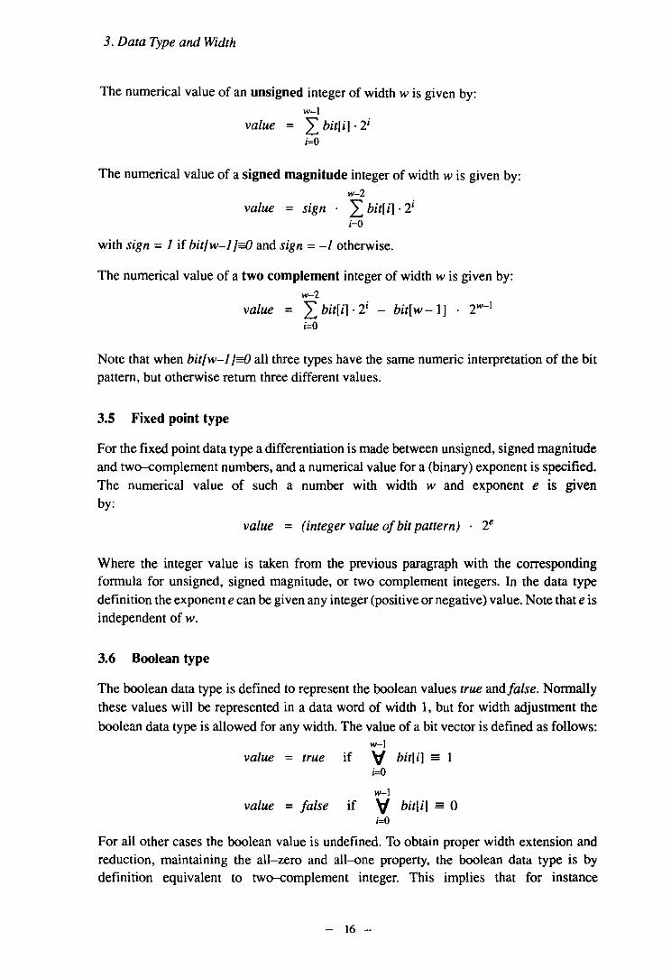
3.5 Fixed point type

For the fixed point data type a differentiation is made between unsigned, signed magnitude and two--complement numbers, and a numerical value for a (binary) exponent is specified. The numerical value of such a number with width wand exponent e is given by:

value = (integer value of bit pattern) . 2<

Where the integer value is taken from the previous paragraph with the corresponding formula for unsigned, signed magnitude, or two complement integers. In the data type definition the exponent e can be given any integer (positive or negative) value. Note that e is independent of w.

3.6 Boolean type

The boolean data type is defined to represent the boolean values true and false. Normally these values will be represented in a data word of width 1, but for width adjustment the boolean data type is allowed for any width. The value of a bit vector is defined as follows:

w-l value = true if V bitli) == 1

i=O

w-l

value = false if V bit!il == 0 i=O

For all other cases the boolean value is undefined. To obtain proper width extension and reduction, maintaining the all-zero and all-{)ne property, the boolean data type is by definition equivalent to two--complement integer. This implies that for instance

- 16 -

true & x ;; x for all bit vectors x, also after width adjustment of true to the width ofx. This property was considered highly desired. As result of having boolean type equivalent to

two-complement integer by definition, the numerical value ofJulse is 0, the numerical value

of true is -I. Or, in the other way around, the two-complement integer values 0 and -I have

the all-O and all-/ property for every width w"?l.

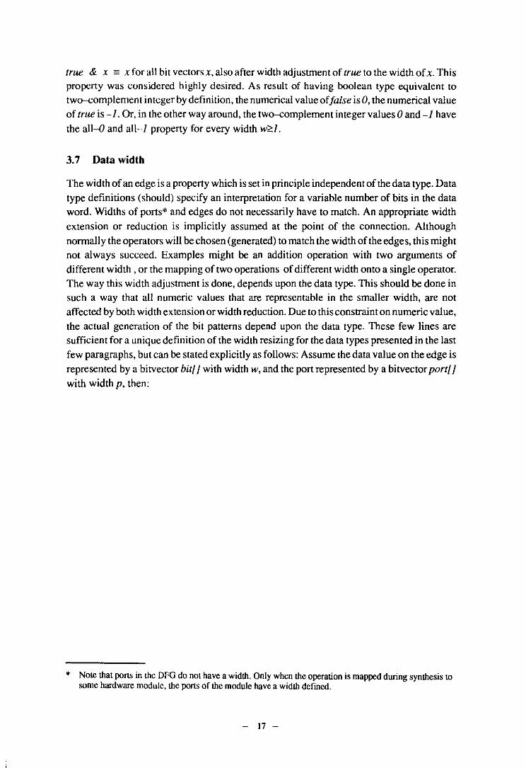
3.7 Data width

The width of an edge is a property which is set in principle independent of the data type. Data

type definitions (should) specify an interpretation for a variable number of bits in the data

word. Widths of ports* and edges do not necessarily have to match. An appropriate width

extension or reduction is implicitly assumed at the point of the connection. Although

normally the operators will be chosen (generated) to match the width of the edges, this might not always succeed. Examples might be an addition operation with two arguments of

different width, or the mapping of two operations of different width onto a single operator.

The way this width adjustment is done, depends upon the data type. This should be done in

such a way that all numeric values that are representable in the smaller width, are not

affected by both width extension or width reduction. Due to this constraint on numeric value,

the actual generation of the bit patterns depend upon the data type. These few lines are

sufficient for a unique definition of the width resizing for the data types presented in the last

few paragraphs, but can be stated explicitly as follows: Assume the data value on the edge is

represented by a bitvector bit!! with width w, and the port represented by a bitvector port!] with width p, then:

• NolC that ports in the DFG do not have a width. Only when the operation is mapped during synthesis to some hardware module, the ports of the module have a width defined.

- 17 -


p<w p>w

unsigned p-l w-l

V port[ i] = bit! i) V port! i] = bit! i] i=O i=O

p-l

V port!iJ = 0 i=w

two-complement p-l w-l

V port(j] = bit(i] V port! i! = bit(i] i=O i=O

p-l

V portti] = bitlw - I] i=w

signed magnitude p-2 w-2

V port[i] = bit[i] V port[i] = bit[ij i=O i=O

port!p -I] = bit[w-l] p-2

V portti] = 0 i=w-l

port[p-IJ = bit[w-I]

No numeric type p-l w-l

just bitvector V port[i] = bit[i] V port[i] = bit[ij i=O i=O

p-l

V port[ij = 0 i=w

Widths and data types have no meaning on edges of type 'source', 'chain', and 'timing', since such edges do not transfer data values, but the presence of tokens only. If a different width adjustment is desired which does not agree with the above table, this can be explicitly created by means of the bit operation nodes.

3.8 Numeric value transfer

The addition of data types and widths to a graph is not just annotating more information, but can -and often wiJI- really change its behavior. Without data types, numeric values are passed along edges without loss of accuracy or range limitations. After addition of data

types, the edges can represent only a finite number of discrete values which can disturb the

data transfer. The process of transferring numeric values is explained as follows: For any numerical result of an operation (including constant nodes), a bitpattern is to be made, representing the value according to the data type of the attached edge, in a width just large enough to accurately represent the value. Then this pattern is taken as 'port' value to be converted to fit the edge width as in the previous table. For a hexadecimal or octal constant, this initial bit pattern has a width just large enough to hold all nonzero bits. This process must be repeated for any edge attached to the output port, since these edges might have different data types or widths. Thus for example the value '3' and patterns 'Ox3' and 'Ox03' all three

lead to the same bit pattern on a two-complement integer edge. If the width of this edge is ;"3, the receiving node obtains the numerical value '3', otherwise it receives the value' -I'. If a

- 18 -

data value cannot be represented in the data type of an attached edge, this is considered a fatal error: numerical values of -3 or 2.5 cannot be assigned to edges of type unsigned integer.

- 19 -

4. Timing

4. Timing

4.1 Introduction

This chapter will discuss timing properties of the data flow graphs and the related seman tical issues. All timing aspects are optional in the graph format: its semantics as algorithmic specification on data values will always remain independent of any timing information. Although optional, timing aspects are extremely important during the synthesis process. Hence the discussion in this chapter cannot be limited to purely behavioural aspects of the graph as model, but time aspects of the underlying -to be synthesized- hardware do appear. To make a distinction between these, we will use time constraints to indicate hard limitations with respect to the timing behavior of a design, imposed by the external world, and we will use time delay to denote a timing property of any hardware used, selected or generated during the synthesis process. The combination of these constraints and delays bounds the search for optimal time-area trade-{)ffs during the synthesis process. Since the constraints can be regarded as real behavioural specifications, they deserve a full and well standardized place in the DFG format and semantics. From this specification point of view the delays basically do not belong to the DFG, since these depend upon chosen hardware, and become known only during the synthesis process. However due to the strong relation between these, we will define a meaning for the delay concept and a textual representation in the format. Treating both will help in discussing the timing concept, and allows more opportunities to exchange design information and compare tool (scheduling) results.

Another timing constraint often imposed by the external world for the design to be synthesized is the system clock cycle time. The DFG syntax allows to express minimum and maximum bounds for this. Of course this is important information for the module selection

and scheduling process.

All absolute timing data such as asynchronous (real time) delays and clock cycle times are expressed as decimal floating point numbers in units of seconds.

4.2 Time intervals

Both for timing constraints and delays a time interval must be specified. For each such specification a choice can be made between either an asynchronous or a synchronous interval specification.

An asynchronous specification provides a single numerical value describing an interval in real time (in seconds).

A synchronous specification provides an integer value, describing a time interval in units of full clock cycles. The synchronous specification optionally contains a leading edge interval in real time (the time required before the first clock transition), and a trailing edge interval in real time (the time required after the last clock transition). It is assumed that these leading and trailing intervals take only a (small) fraction of the actual clock cycle time. A clock cycle value of n>O means that the interval contains n full clock cycles plus the optional leading and

- 20 -

trailing intervals, a clock cycle value of 0 means that the interval contains just a clock edge with the leading and trailing intervals. As special exception the number of cycles can be specified as -I, meaning that the number of cycles is unknown (cannot be determined at compile time), and can depend upon the involved data values.

4.3 Constraint specification

Timing constraints are specified as (optional) properties of edges of type timing. These edges are added to the graph for the sole purpose of capturing time information. They participate as other edges in the process of token passing, only the data value on the tokens is ignored. A timing edge without a constraint specification hence introduces an extra constraint on the execution ordering of the attached nodes. A minimum timing constraint can be added to specify that the destination node should never be executed within a certain time interval from the execution of the originating node. Equivalently it is considered an error when any token stays shorter on a timing edge than a specified minimum timing constraint. A maximum timing constraint can be added to specify that the destination node must be executed within a certain time interval from the execution of the originating node. Equivalently it is considered an error when any token stays longer on the edge than the specified maximum timing constraint. Due to their nature of being constraints on the behavior of a graph, these edges will normally appear between input and output nodes or between get and put nodes of a graph. However they are allowed between any two nodes.

0) 0) chain edge ' , chain edge

~ liming , ~_edge - '

--~ --

chain edge:

, ---~ timing ~ edge chain edge

. ---e -~

Figure ll. Ordering constraints between I/O operations on two ports

4.4 Delay specification

Figure 12. Constraints on the graph execution time

Delay specifications will normally be used forthe nodes in the graph. Values forthesedelays are assumed to be inherited or fetched from a module library, as a result from a module

- 21 -

4. Timing

selection process. Both minimum and maximum delays are supported: A minimum delay is at least consumed by the node before generating an output token, a maximum delay is the time interval in which an output token will certainly be generated. Of course these are not both required: if only one (nominal) delay value is available the maximum entry will normally be specified. Delays are also allowed on edges although this probably has minor use.

4.5 The timing model

For an accurate specification of the timing behavior of the graph the execution model is explained. When delay values are inserted in the graph, the graph execution can reveal timing information, however remind that the basic reason to introduce these delays is to inform a scheduling algorithm. Besides a numerical and/or bitpattern value, each token now carries a time point. In principle this time point has two component.~: an integer number indicating the current clock cycle, and a number giving a real time delay after the last clock edge. If the clock cycle time is known, these two can of course be combined into one number, either in absolute real time or relative with respect to the cycle time. The time value carried by any token is normally the point in time where the token became available at the output of a node. If edge delays are specified, this time point is accordingly updated before the token appears at the edge destination (a node input).

Any primitive node will generate an output token at a time point of its delay later than the arrival of the last input token. If both a minimum and a maximum delay are available for the node with different values, an undeterministic time point results from this interval.

Any node corresponding to the instantiation of a graph passes its input tokens unmodified to the input nodes of the graph definition. This subgraph is then executed and tokens appearing at output node(s) are passed again to the corresponding output port(s) of the instantiating node. This implies that a delay specification for such a node is actually ignored. The resulting timing behavior of such a node is hence basically different from a primitive node: An instantiating node with for instance three inputs and two outputs might generate a token at its first output at a time point where the third input token has not yet arrived! Such behavior does not conflict with the execution mechanism as presented in section 2.2: timing just adds information to these tokens. As result of this timing model, expanding the instantiating node (replacing it by its graph definition) does not modify the timing behavior of the graph.

During the graph execution a minimum timing constraint is violated if a token resides shorter on the (timing) edge than the specified interval, a maximum timing constraint is violated if a token resides longer on the (timing) edge than the specified interval.

Note that such a graph execution to reveal timing properties would not reflect real hardware behavior: The data flow graph is still a maximal parallel representation, and the presented execution scheme hence assumes unlimited hardware resources. Only after the architectural synthesis is completed, scheduling and module allocation results would allow a simulation based on a hardware structure. The extension of incorporating the results of scheduling and allocation in the DFG, is outside the scope of (this release of) this manual.

- 22 -

4.6 Ripple delay

To refine the timing model in the DFG an extension is made to use information regarding ripple delays as found in many arithmetic operations. A ripple delay is defined as the time interval that elapses between the generation or use of successive bits in a bitvector, generated by or used in an operation. The influence on the timing of operations is illustrated

in Figure 13. and Figure 14.

DFG caption

\ width = 8

delay = 9 +

width = 8

& delay = 1

width = 8

delay = 9

width = 1

Module activity

msb data bits Isb o -r--,------.,...

time

1

9 10

19

+-_ adder

bitwise and

comparator

Figure 13. Timing without ripple delay

The timing properties of the graph with ripple delays is defined by describing the timing

information (conceptually) stored in the data tokens and their firing rules. In thew previous

section it was described that tokens do carry the time point of their creation. When ripple delay is added to (some) nodes, the tokens also obtain a ripple delay value.

Suppose a token is available at each input of a node which has a ripple delay statement

attached, T is the maximum of the timepoints in these tokens, .1 is the maximum of the ripple

delay values in these tokens, dis the node delay, Ii is the node ripple delay, and finally wis the

width of the outgoing data edge. Now the node creates an output token on the outgoing edge

at (with) timepoint T +d-(w-J )xli, and with a ripple delay value of max( .1, Ii). In words: the output token obtains a time point which corresponds to the availability of the least significant bit. The availability of the higher order bits is denoted by the ripple value in the output token.

- 23 -

4. Timing

DFG caption

\

width=8

delay = 9 + ripple-delay = 1

width = 8

delay = 1 & ripple-delay = 0

width = 8

delay = 9 <= ripple-de lay = 1

width = 1

Module activity

msb data brts Isb 0,--------.-

time

! 9

10

12

-1-_ adder

brtwise and

comparator

Figure 14. Timing with ripple delay

If a node cannot cope with the delayed arrival of the higher order bits, this is indicated by not

specifying its ripple delay statement. This causes the node execution to wait until all bits are

available. Suppose each input token has a timepoint Ti, a ripple delay ""i, and width Wi, and d

is the node delay, the output token obtains the timepoint d+max(Ti+(Wi-1 )xill)) and ripple

delay value of O. Thus be aware that specifying a zero ripple delay is intentionally different from not specifying it.

- 24 -

5. Textual Format for the Data Flow Graph

5.1 A flexible format

For an easy interface to various programming languages, we propose a text (ASCII) based format. This has the additional advantage of easy transfer between different machines. The Lisp and EOIF syntax style using a pair of braces for each keyword ensures simple parsing: any LL-l parser is strong enough, such as a recursive descent parser scheme. It furthermore allows for local and future extensions to the format, without disturbing already existing software (both upwards and downwards compatibility), and does not require a set of reserved words, forbidden as identifier.

The basic format is very simple: every object is represented as a list. Any list starts with an opening brace and a keyword on which the application determines its interest in the list. The items of the list are names, numbers and other lists, and the list is terminated with a closing brace. If an application is not interested in the information attached to the keyword -{)rdoes not recognize the keyword- it can and should skip this list without knowing anything about its (structured) contents by just counting braces.

Of course for successful exchange of data flow graphs between various systems a minimal subset of required data, keywords and type names must be agreed upon. However every tOOl/site is free to add more data for its own purpose. If project partners make such local

extensions which might be useful to others as well, effort must be started to agree on their

use.

5.2 Lexical analysis

For the lexical analysis of the input text the following rules can be stated:

• So called' white space' serves as delimiter, and consists of one or more of the following characters: space' " tab '\t', linefeed '\n', carriage-return '\T', and formfeed '\f'. All keywords, names and numbers have to be separated by white space. The previous

release of this manual stated that no white space was required around 'C and ')'. However from now on, we strongly advise to create white space around identifiers. In future releases this will probably become mandatory, and files without such spacing might become impossible to read with future lexical analyzers. The reason for demanding white space is that it both eases (speeds up) the lexical analysis as well as removes unnatural restrictions on identifier syntax.

• Case is significant, and all text processing and keyword matching is done case sensitive.

• Comment statements as defined later can appear anywhere as argument in a list, and is assumed to be removed by the lexical analyzer before matching to the syntax rules is done by the parser. Comment statements can nest. •

- 25 -

I

5. Textual Format for the Data Flow Graph

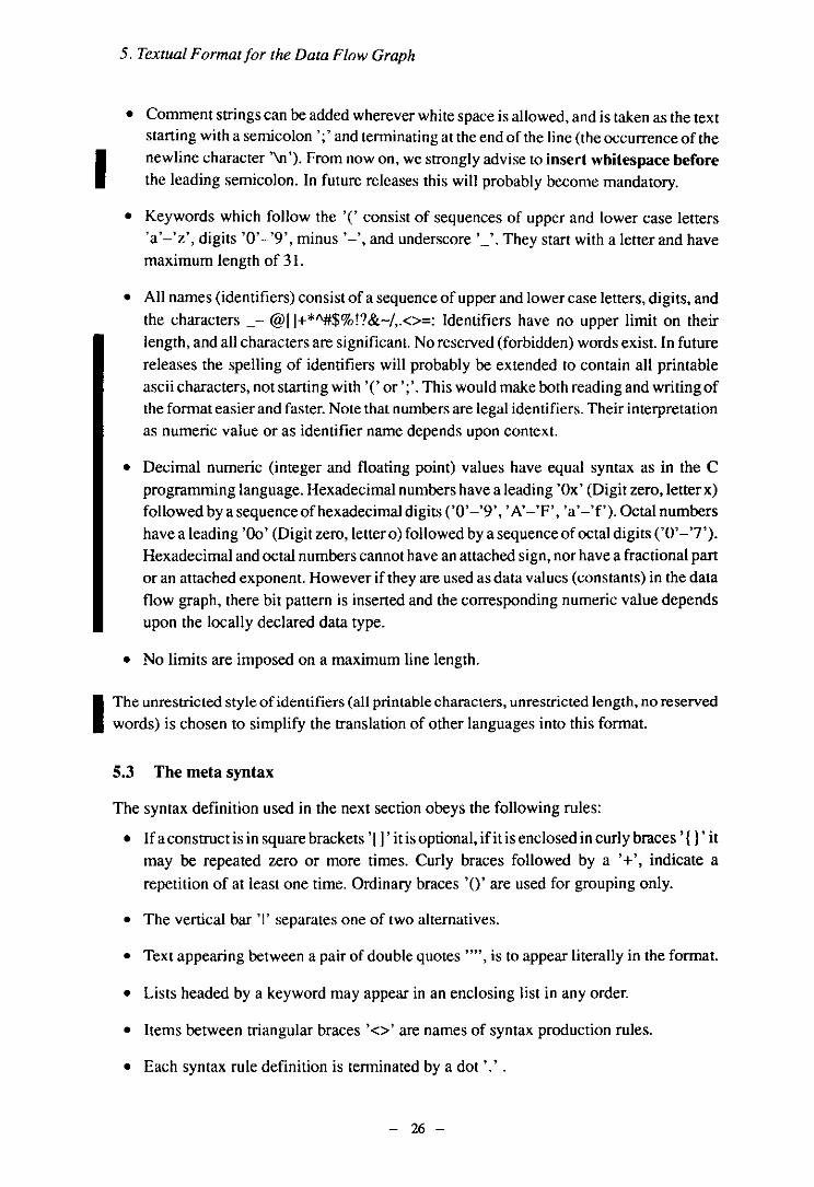
• Comment strings can be added wherever white space is allowed, and is taken as the text starting with a semicolon ';' and terminating at the end of the line (the occurrence of the newline character '\n '). From now on, we strongly advise to insert whitespace before the leading semicolon. In future releases this will probably become mandatory.

• Keywords which follow the '(' consist of sequences of upper and lower case letters 'a'-'z', digits '0'-'9', minus' -', and underscore '_'. They start with a letter and have maximum length of 31.

• All names (identifiers) consist of a sequence of upper and lower case letters, digits, and the characters _ - @II+*"#$%!?&-/,.<>=: Identifiers have no upper limit on their length, and all characters are significant. No reserved (forbidden) words exist. In future releases the spelling of identifiers will probably be extended to contain all printable ascii characters, not starting with '(' or ';'. This would make both reading and writing of the format easier and faster. Note that numbers are legal identifiers. Their interpretation as numeric value or as identifier name depends upon context.

• Decimal numeric (integer and floating point) values have equal syntax as in the C programming language. Hexadecimal numbers have a leading 'Ox' (Digit zero, letterx) followed by a sequence of hexadecimal digits ('0' -'9', 'A' -'F', 'a' -'f'). Octal numbers have a leading '00' (Digit zero, letter 0) followed by a sequence of octal digits ('0'-'7').

Hexadecimal and octal numbers cannot have an attached sign, nor have a fractional part or an attached exponent. However if they are used as data values (constants) in the data flow graph, there bit pattern is inserted and the corresponding numeric value depends upon the locally declared data type.

• No limits are imposed on a maximum line length.

I The unrestricted style of identifiers (all printable characters, unrestricted length, no reserved words) is chosen to simplify the translation of other languages into this format.

5.3 The meta syntax

The syntax definition used in the next section obeys the following rules:

• If a construct is in square brackets 'I]' itis optional, if it is enclosed in curly braces' { J' it may be repeated zero or more times. Curly braces followed by a '+', indicate a

repetition of at least one time. Ordinary braces '0' are used for grouping only.

• The vertical bar 'I' separates one of two alternatives.

• Text appearing between a pair of double quotes "", is to appear literally in the format.

• Lists headed by a keyword may appear in an enclosing list in any order.

• Items between triangular braces '<>' are names of syntax production rules.

• Each syntax rule definition is terminated by a dot'.' .

- 26 -

The general form of any statement is:

<statement> ::= "(" keyword {identifier I <statement> } ")".

The general rule is that a statement begins with ( keyword and is followed by a list of arguments. These arguments can be statements or basic items such as numbers and identifiers. These basic items have a fixed position (order). Statements may appear in any order because they are identified by their keyword.

It is implicitly assumed that any statement allows the comment statement as argument. The comment statement is identified by the keyword comment. Thus a comment statement is build as follows:

<comment-statement> ::= "(" "commenf' { identifier I <statement> } ")".

5.4 The DFG syntax definition

The DFO is now defined by the following syntax rules:

<DFGview>

<Design>

<Graph Ref> '

<DataTypeDef>

::= "(" "dig-view" [<Design>] {<DataTypeDef>} {<DataTypeDefaull>} {<Graph>}+ ")".

::= "(" "design" <Graph Ref> ")".

::= "(" "graph-ref" <Graph Name> ")".

::= "(" "datatypedef" <DataTypeName> [<DataTypeSpec>] <Width Default> ")".

<DataTypeName> ::= <identifier>.

All data type names in one dfg-view must be unique.

<DataTypeSpec>

<lntegerType>

::= <lntegerType> I <FixedpointType> I <BooleanType>.

::= "(" ( "integer-unsign" I "integer-2compl" I "integer-signmagn" ) ")" .

<FixedpointType> ::= "(" ( "fixpoint-unsign" I "fixpoint-2compl"l "fixpoint-signmagn" ) <FixedpointExp> ")".

<FixedpointExp> ::= <integer>.

<BooleanType> ::= "(" "boolean" ")".

<DataTypeDefault> ::= "c "datatype-default" <EdgeTypeName> <DataTypeName> It) ".

<Width Default> ::= "(" "width-default" <integer> ")".

<Graph>' ::= "(" "graph" <Graph Name> {<Node> I <Edge>} [<status>] [<MinCycietime>] [<MaxCycietime>] [<BoundingBox>j")".

<Graph Name> ::= <identifier>.

All graph names in one dfg-view must be unique.

<BoundingBox> ::= "(" "bbox" <XCoord> <YCoord> ")" .

<XCoord> ::= <integer>.

<YCoord> ::= <integer>.

X-coord and y-coord must be greater than zero.

- 27 -

•

•

5. Textual Format/or the Data Flow Graph

<status>

<written>

<timestamp>

<author>

<program>

<MinCycletime>

<MaxCycletime>

<Node>'

<NodeName>

::= "(" "status" { <written> } ")".

::= "(" ''written'' <timestamp> <author> <program> ")" .

::= <identifier>.

::= <identifier>.

::= <identifier>.

::= "(" "min-cycletime" <number> ")".

::= "(" "max-cycletime" <number> ")".

::= "(" "node" <NodeName> <NodeType> [<In Edges>] [<OutEdges>] [<Selection List>] [<ConstValue>] [<Varname>] [<Srcline>] {<Position>} [<ScheduleTime>] [<ArrayDim>] [Min Delay] [MaxDelay]"}".

::= <identifier>.

All node names in one graph must be unique.

<NodeType> ::= "(" "type" <NodeTypeName> ")".

<NodeTypeName> ::= <identifier>.

Node types are either implicitly predefined types or names of graphs defined elsewhere in

the file.

<lnEdges>

<OutEdges>

<EdgeName>

::= "(" "in-edges" { <Edge Name> }+ ")".

::= "(" "out-edges" { <Edge Name> }+ ")".

::= <identifier>.

The edge name must refer to an edge definition elsewhere in the graph.

<SelectionLisl>' ::= "(" "selection-list" {<integer>)+ ")".

A selection list has meaning for 'entry', 'exit', 'merge', and 'branch' nodes only.

<ConstValue>' ::= "(" "const-value" {<number>}+ ")".

The const-value attribute has meaning for node types 'constant', 'array', 'entry', and

'delay' only.

<ArrayDim> ' ::= "(" "array-<Jim" {<integer>}+ ")".

I The array-<Jim attribute has meaning for node type 'array' only. The number of integers

determines the number of dimensions. Each integer specifies the size of one dimension, and

must be greater than zero.

<Var-name> ::= "(" ''varname'' <identifier> ")".

<Srcline> ::= "(" "src-line" <identifier> ")".

<Position> ::= "(" "position" <XCoord> <YCoord> ")".

X-<:oord should have a value between zero and the bbox( x-<:oord), bounds inclusive. Ycoord should have a value between zero and the bbox( y-<:oord), bounds inclusive.

<ScheduleTime>' ::= "(" "schedule-time" <number> ")".

<Edge> ::= "(" "edge" <Edge Name> <EdgeType> <Origin> <Destination> [<DataType>] [<Width>] [<Varname>] [<MinDelay>] [<MaxDelay>] [<MinTime>] [<MaxTime>] ")".

* These synlax slatements are extended in chapter 6. on parameterization.

- 28 -

<EdgeName> ::= ddentifier>.

All edge names in one graph must be unique.

<Edge Type> ::= "(" "type" <EdgeTypeName> ")".

<EdgeTypeName> ::= <identifier>.

Edge types are implicitly predefined.

<Origin> ::= "C' "origin" <NodeName> [<Port>]")".

<Destination> ::= "(" "destination" <NodeName> [<Port>]")".

The node names must refer to a node definition elsewhere in the same graph.

<Port>

<PortName>

::= "(" "port" <PortName> ")".

::= <identifier>.

Portnames are implicitly predefined for predefined node types. If the referred node has a type which is defined as graph elsewhere, they must agree with names of input and output nodes of that graph.

<Width>' ::= "C' ''width'' <integer> ")".

The width must be greater than zero. The attribute has meaning for edge types 'data' and 'control' only.

<DataType>' ::= "C' "data-type" <identifier> ")".

The data type name must refer to data typedef elsewhere in the file.

<Min Delay> ::= "C' "min-<lelay" <Timelnterval> [<Ripple Delay>] ")".

<Max Delay> ::= "C' "max-<lelay" <Timelnterval> [<RippleDelay>] ")".

<RippleDealy> ::= "(" "ripple-<lelay" dime Interval> ")".

<MinTime> ::= "(" "min-time" <Timelntervai> ")".

<MaxTime> ::= "(" "max-time" <Time Interval> ")".

< Timelnterval> ::= <Asynclnterval> I <Synclnterval> .

<Asynclnterval>' ::= "(" "async" <number> ")".

<Synclnterval>' ::= "(" "sync" <integer> [<LeadDelay>] [daiIDelay>] ")".

<LeadDelay>' ::= "(" "Iead-<lelay" <number> [<ClockPhaseld>] ")".

<Tail Delay>' ::= "(" "tail-<lelay" <number> [<ClockPhaseld>] ")".

<ClockPhaseld>' ::= <integer>.

The definition starts with the definition of a view for the set of data flow graphs. At file scope data types are defined. The design statement indicates which graph is to be taken as the current object of design and the root of the hierarchy. The graph has a name, a set of nodes and a set of edges. The names of the graphs in one view must be unique, and can be referred to as nodetype in another graph for instantiation. For each node its incoming and outgoing edges are specified. Other attributes are a node-name to identify the node and a type to describe which operation is performed by the node. Two attributes are added to find the

* These syntax statements arc extended in chapter 6. on parameterization.

- 29 -

•

5. Textual Format/or the Data Flow Graph

correspondence between the graph and its original (user-<:ontributed) algorithmic

description in another language: the src-line gives the line numberofthe source code where an operation was described and the varname describes the output variable of the node. These last two attributes are especially useful to infornl the user about the graph. (for example in generating error messages).

For each edge its origin node and destination node are specified. Optionally port names can be attached here, required to distinguish between the inputs of noncommutative operations or between the outputs of multioutput operations. Further attributes are an edge-name to

identify the edge and a type to give the edge its type. The varname attribute is used to relate the edge to a variable name used in the input specification.

More graphs can be described in a single file by listing several graphs in one file.

Attributes concerning the author, source program, date etcetera are optionally collected in the status field.

5.5 Predefined node types

For a useful DFG exchange, a set of node types and their semantics must be agreed upon.

For the arithmetic operators we adopt the C language notation as type name. All these 'C' operators have only one output port (to which of course multiple edges can be attached). The commutative operations are assumed with an undetermined number of inputs, but at least two. For these operations port names are not explicitly defined, since there is no need to do so. The non-<:ommutative operations are defined fortwo inputs, with their input port names. The unary numeric negate operation has obtained type 'neg' to distinguish it from the dyadic

I subtract operation with type' -'. If a 'boolean result' is specified for the operations, this means that the result of the operation (the output token) has a numeric value of either 0 (false) or -I (true).

The predefined node types are:

Numeric operations:

+

* /

%

numeric addition, undetermined number of inputs.

numeric multiplication, undetermined number of inputs.

numeric divide, two arguments, input ports 'left' and 'right'.

numeric modulo, two arguments, input ports 'left' and 'right'.

numeric subtract, two arguments, input ports 'left' and 'right'.

neg numeric negation, one argument.

++ numeric increment, one argument.

numeric decrement, one argument.

- - comparing its arguments, numeric or bitvector, boolean result, undetermined number of inputs.

- 30 -

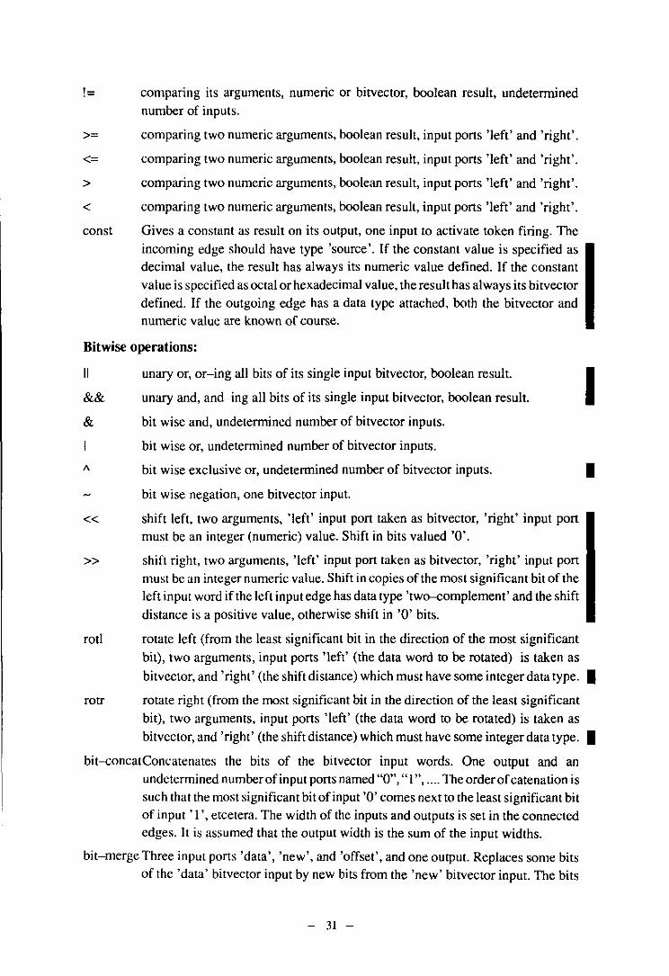
!= comparing its arguments, numeric or bitvector, boolean result, undetermined number of inputs.

>=

<=

>

<

const

comparing two numeric arguments, boolean result, input ports 'left' and 'right'.




Gives a constant as result on its output, one input to activate token firing. The incoming edge should have type 'source'. If the constant value is specified as decimal value, the result has always its numeric value defined. If the constant value is specified as octal or hexadecimal value, the result has always its bitvector defined. If the outgoing edge has a data type attached, both the bitvector and numeric value are known of course.

Bitwise operations:

II

&& unary or, or-ing all bits of its single input bitvector, boolean result.

unary and, and-ing all bits of its single input bitvector, boolean result.

& bit wise and, undetermined number of bitvector inputs.

bit wise or, undetermined number of bitvector inputs.

1\ bit wise exclusive or, undetermined number of bitvector inputs.

bit wise negation, one bitvector input.

« shift left, two arguments, 'left' input port taken as bitvector, 'right' input port must be an integer (numeric) value. Shift in bits valued '0'.

» shift right, two arguments, 'left' input port taken as bitvector, 'right' input port must be an integer numeric value. Shift in copies of the most significant bit of the left input word if the left input edge has data type 'two--complement' and the shift distance is a positive value, otherwise shift in '0' bits.

I

•

rot! rotate left (from the least significant bit in the direction of the most significant bit), two arguments, input ports 'left' (the data word to be rotated) is taken as

bitvector, and' right' (the shift distance) which must have some integer data type. •

rotr rotate right (from the most significant bit in the direction of the least significant bit), two arguments, input ports 'left' (the data word to be rotated) is taken as bitvector, and 'right' (the shift distance) which must have some integer data type. •

bit-concatConcatenates the bits of the bitvector input words. One output and an undetermined number of input ports named "0", ")", .... The order of catenation is such that the most significant bit of input '0' comes next to the least significant bit of input ') " etcetera. The width of the inputs and outputs is set in the connected edges. It is assumed that the output width is the sum of the input widths.

bit-merge Three input ports 'data', 'new', and 'offset', and one output. Replaces some bits of the 'data' bitvector input by new bits from the 'new' bitvector input. The bits

- 31 -

5. Textual Formatfor the Data Flow Graph

are selected in the 'data' word by an 'offset' numeric input. The value of the 'offset' token (integer> 0), indexes the 'data' word, such that the least significant bit is numbered '0'. The thus indicated bit in 'data' is replaced by the least significant bit of the 'new' input; the next higher bit of 'data' is replaced by the next bit of 'new', etcetera, forthe full length of the 'new' input. The width of the

arguments is set in the attached edges. It is assumed that the width of the output is equal to the width of the 'data' input, and that the 'new' input has smaller width than these.

bit-select selection of a bit range from a variable (bus). One bitvector input 'data' and one numeric input 'offset'. The value of the 'offset' token (integer> 0), indexes the input word, such that the least significant bit is numbered '0'. The least significant bit of the output word corresponds to bit 'offset' of the input word. Note that the width of input and output data are determined by the connected edges, where the output width is assumed smaller than the input data width.

Control nodes:

branch To build 'if-then-else' constructs, see section 2.5. Two inputs 'data' and 'control', multiple outputs named '0', '1', '2', ... Because one incoming edge

should have type' control', the input port names are optional to use. A selection

list is given for each branch node. This is an ordered list of all different data values. The value of a data token arriving at the control input is compared with

each value in this list. The index of the matching value*, defines the output port

which will receive the token from the data input.

merge

entry

To build 'if-then-else' constructs, see section 2.6. One output port 'data', multiple input ports named 'control', '0', , I', ... The edge connected to 'control'

should have type 'control'. A selection list is given for each merge node. This is an ordered list of all different data values. The value of a data token arriving at the

control input is compared with each value in this list. The index of the matching value*, defines the input port which will receive a token to pass to the data output.

To build loop constructs, see section 2.7. One output port 'data', multiple input ports named 'control', '0', '1', ... The edge connected to 'control' should have

type 'control'. A selection list is given for each entry node. This is an ordered list of all different data values. The value of a data token arriving at the control input

is compared with each value in this list. The index of the matching value*, defines

the input port which will receive a token to pass to the data output.

exit To build loop constructs, see section 2.7. Two inputs' data' and 'control', multiple

outputs named '0', '1', '2', ... Because one incoming edge should have type 'control', the input port names are optional to use. A selection list is given for

------• Comparison for (in-)cquality is legal for both numeric values and for bit veClOrs. If data types and

I widths are defined, values and bit veclOrs can be convened in to each olher, and then the comparison must be done for the bit vectors, as normal for all operations. Thus the data value in the selection list is convened to a bitpattcm according to the data type and width of the control edge, and then compared with the control token. This implies for instance that a control edge of type two--complcmcnt integer of width I, will match the numeric values' I' and '-I' as equaL

- 32 -

each exit node. This is an ordered list of all different data values. The value of a data token arriving at the control input is compared with each value in this list. The index of the matching value*, defines the output port which will receive the token from the data input.

noop an operation which actually does nothing. It might be used for just adding precedence or timing relations, with an undetermined number of inputs (> I):

delay

The operation waits until a token is available on each input, and then generates some output token. However its real semantics with respect to token data values is ONLY defined for its usage with a SINGLE input edge. In this case it passes the input token -with its value- to its output port. In this situation the node might be used for structuring of edges, for whatever reason. No restrictions apply to the type of edges which attach to this node.

The delay node has one 'data' input and one 'data' output port. Any token arriving at the input is just passed to the output port. However a 'const-value' statement can be attached to this node, containing a list of values. All these values are -in order- made available as tokens on the output port at initialization time. Hence new tokens arriving at the node input are queued behind this list. As result, this node can be used to obtain access to data values from previous executions of the graph (previous cycles of the implicit external loop).

Input and output:

get To read data from external ports, see section 2.8. One input to activate the reading process, thereby producing an output token on its single output port. The input edge should have type 'chain', there must be precisely one output edge of type 'chain', besides the normal outgoing data edges.

put to write data to external ports, see section 2.8. Two input ports named 'enable' and 'data', one output port named 'enabled'. The edge connected to 'enable' is used to activate the reading process, and should have type 'chain'. The (single) edge connected to 'enabled' must also have type 'chain', and is used to start the next I/O operation on the same external port.

input

output

input interface node for any graph. Its node name serves as port name when this graph is called (instantiated) in another graph. No input ports, one output port.

output interface node for any graph. Its node name serves as port name when this graph is called (instantiated) in another graph. No output ports, one input port.

Array operations:

array declaration of an array, see also the general description in section 2.9. One input port 'source', used to 'activate' the array declaration and initialization, an edge of type 'source' should be attached to this port. Outgoing' chain' type edges provide access to and specify a (partial) ordering of all update and retrieve operations accessing this array. These 'chain' edges don't have port references. The array I dimensionality and its size in each dimension must be specified. An initialization

- 33 -

5. Textual Formatfor the Data Flow Graph

with (constant) values is optional. This linear sequence of constant values is written in the array with 'highest index running fastest' order. If too few values are specified, the rest is left initialized, if too many values are specified, the excess values are ignored.

retrieve read access to a value of an array, see also the general description in section 2.9.

update

This node has input ports implicitly named '0', , I " '" used to connect incoming edges to index the array (address one element), which is written at the output port named' data'. The node has furthennore one or more incoming and zero or more outgoing edges of type' chain' , to connect and order the read and write operations on the array. The port names '0', , I " ... and 'data' must be mentioned explicitly on its connected 'data' edges, the 'chain' edges cannot have an explicit port indication. The data values to index the array must have nonnegative integer values.

write access to a value of an array, see also the general description in section 2.9. This node has input ports implicitly named '0', , I " '" used to connect incoming edges to index the array (address one element). At this index the array is updated with the value read from the input port named 'data'. The node has furthermore one or more incoming and zero or more outgoing edges of type' chain', to connect and order the read and write operations on the array. The port names '0', , I " ... and 'data' must be mentioned explicitly on its connected 'data' edges, the 'chain' edges cannot have an explicit port indication. The data values to index the array must have nonnegative integer values.

5.6 Predefined edge types

data The 'default' type for edges involved in data transfer. A data edge can have a data

type and a width attached.

control Edges of type control are always connected to the 'control' input of branch, merge, entry or exit nodes. Its use is to be able to distinguish these edges from the 'data' type, for synthesis or drawing reasons, although they behave identically. These edges will connect all branch and merge nodes of one 'if' statement or all entry and exit nodes of one loop statement to a single node generating the control. In the resulting hardware these edges will often lead to wiring from a 'controller' module. A control edge can have a data type and a width attached.

chain Any chain edge belongs to a sequence that serially links all put and get nodes that operate on one physical external communication port. Note that this chain should go through branch, merge, entry, and exit nodes and procedure instantiations if get and put nodes are inside these constructs. Each such chain should start at an 'input' node and tenninate at an 'output' node. Also used to connect together and define a partial order between between 'array', 'retrieve', and 'update' nodes, forming a connected acyclic graph with these nodes. In the array specification, 'input' and 'output' nodes are not involved, but these chains can also go through branch, merge, entry, and exit nodes, and procedure instantiations if retrieve and update nodes are inside these constructs.

- 34 -

source

timing

input edge to a node of type 'constant' needed to enable the 'firing' of its output token containing its constant value, or input edge toa node of type 'array', needed to activate its initialization and firing of tokens on its 'chain' outputs.

These edges are used to enforce a required timing or execution ordering on the nodes in the DFG. Forthis purpose they can havea 'delay' statement, prescribing a (minimal) time difference between the completion of its originating and start of its destination node.

Other operations:

All other node types encountered are assumed to be instantiations of graphs defined elsewhere in the file. The node type name must hence correspond to the graph name. The ports of the node at instantiation must correspond with the input and output nodes of the graph. Note that the previously listed predefined nodes do not create a reserved or illegal set of graph names: They are also legal graph names, allowing the redefinition of standard operators.

- 35 -

6. Parameterization

6. Parameterization

6.1 Introduction

The chapter on parameterization is new in this release. Therefor comments on desired improvements and modifications are welcome.

The need for parameterization in the DFG format was apparent for some time already. The two main reasons for this are:

• Actual parameter assignment at the nodes of a graph is necessary to direct or control the generation of hardware operators.

• It should be possible to define a graph which is parameterized for (at least) the width of its edges.

Parameter passing concepts can lead to an enormous amount of extra syntax and constructs in a language. We felt that the DFG as exchange format, in contrast to a user interface language, would be better served with a syntactically minimal but still general enough scheme. Due to the keyword driven nature of the DFG format, extension remains possible of course. These considerations based the following choices:

• Nodes can have attached actual parameter assignments.

• Graphs can have formal parameter declarations. Together with the parameter assignment at nodes, this allows passing of parameters through a hierarchy of DFGs.

• Various places where only a constant number or identifier was allowed, now allow an expression. If for example a graph has a parameter w, some edges can have assigned a width w, others a width w+ 1 orwx2. For now only a small set of expression operators is defined.

• Parameters do not have a data type nor a structure. This greatly simplifies implementation. Whatever is assigned to a parameter, is just inserted when the parameter is used.

• Parameters are local to the graph where they are declared. Their names are unique in each graph. Therefor no scoping rules supporting concepts as name hiding need to be implemented.

• Parameters cannot influence the connection structure of a graph. They cannot lead to deletion or insertion of edges or nodes.

6.2 Extended syntax

The extension of the format is now defined as:

<Graph Ref> ::= "(" "graph-ref" <Graph Name> {<ParamAsg>} ")".

- 36 -

<Graph>

<ParamDecl>

<ParamName>

::= "(" "graph" <Graph Name> {<Node> I <Edge> I <ParamDeci>} [<status>] [<BoundingBox>]")".

::= "(" "param-deci" <ParamName> <ParamDefauItValue> ")".

::= <identifier>.

Parameter names are unique in a graph. They do not interfere with other names.

<ParamDefauItValue> ::= <identifier>;

Note that numbers are also identifers. Their interpretation as number depends upon context.

<Node>

<ParamAsg>

<SelectionLisb

<ConstValue>

<ArrayDim>

<Schedule Time>

<Width>

<DataType>

<Asynclnterval>

<Sync Interval>

<Lead Delay>

<TaiiDelay>

<ClockPhaseld>

<Expr>

<ParamEvai>

<MonadicExpr>

<MultiadicExpr>

::= "(" "node" <NodeName> <NodeType> [<lnEdges>] [<Out-Edges>] [<Selection-Lisb] [<ConstValue>] [<Varname>] [<Src-line» {<Position>} [Schedule-time) [<Array-dim» [Delay) {<ParamAsg>} ")".

::= "(" "param-asg" <ParamName> <Expr> ")".

::= "(" "selection-iist" {<Expr>}+ "}".

::= "(" "const-value" {<Expr>}+ "}".

::= "(" "array-dim" {<Expr>}+ ")".

::= "(" "schedule-time" <Expr> "}".

::= "(" ''width'' <Expr> "}".

::= "(" "data-type" <Expr> "}".

::= "(" "async" <Expr> ")".

::= "(" "sync" <Expr> [<LeadDelay» [daiIDelay» ")".

::= "(" "Iead-delay" <Expr> [<ClockPhaseld» ")".

::= "(" "tail-delay" <Expr> [<ClockPhaseld>] ")".

::= <Expr>.

::= <identifier> I <ParamEval> I <MonadicExpr> I<MultiadicExpr>.

::= "(" "evaluate" <ParamName> ")".

::= "(" ( "negate" I "fix" ) <Expr> ")".

::= "(" ( "sum" I "subtract" I "product" I "divide" I "mod" I "min" I "max" ) {<Expr>}+ ")".

Note that we have not yet defined boolean operations in expressions, bitwise logical operations or string operations. Of course these are easily added if so desired.

Because parameters do not have types (integer, number, string) defined by syntax, expressions are also not typed. The notion that "data-type" expects a name as argument, and "array-dim" expects positive integers as argument is hence lost in the syntax. These restrictions can be seen in section 5.4 where the syntax was initially defined.

Specifying a default value for parameters is mandatory. As result a graph is always a meaningful object of its own. Actual parameter assignments of course override this default, and do not need to specify all declared parameters.

The expression operations are inspired by the EDIF version 2.0.0 ANSIJEIA standard, and numerically defined as follows:

- 37 -

6. Parameterization

negate

fix

sum

subtract

product

divide

mod

min

max

Performs the numeric negation of its argument, multiplies with -1.

Truncates its numeric argument to an integer, in the direction of O. For example 2.3 and 2.9 are both converted to 2, and -1.9 is converted to -1.

Performs the numeric summation of its arguments.

Takes its first argument and subtracts all subsequent arguments from it.

Multiplies all its arguments.

Takes its first arguments and divides it by all subsequent arguments. It can produce a fractional result from integer arguments.

Takes its first argument, and performs the modulo operation with all subsequent arguments. All arguments must be integer and the result is integer. If r~(mod a b) and d~(fix (divide a b)) then

a=(sum (product b d) r) and (thus) r has the same sign" as a.

Returns the minimum value of all its arguments.

Returns the maximum value of all its arguments.

• Be warned that the C language leaves the sign of the % operator implementation dependent.

- 38 -

7. Possible Extensions

The discussion on future ordesireful extensions is always required to maintain a high quality and up to date standard, serving every site as good as possible.

In Eindhoven we will very soon start to use extensions of this DFG format, which annotate the results of scheduling and allocation in the data flow graph. This will be done by adding with each data flow graph a ' control graph' -defining a controller finite state machine- and a 'network graph' -specifying the resulting network after module allocation-. If these extensions are acceptable and thought useful by others, they would open up the exchange of individual synthesis tools from the project partners, and hence allow a much tighter cooperation in the project. Such extensions are now in the (software) development stage. The corresponding extension fo the format might initially appear as appendix to this manual.

Although the extension with data types is a large step in the direction of defining a bit-level behavior of the data flow graphs, a bit-wise definition ofthe operation nodes in the graph is still missing. Although the numerical types and their bit patterns do define the 'normal' numerical behavior up to the bit level, exception handling for conditions as overflow are not standardized. By now we assume that each site -{)r even each design- has such a bit-level definition of the operators, which is supported by simulation and module synthesis. Fixing the behavior to a single definition is unacceptable, denying real ASIC design. Alternatively

a method for exchanging the bit-level behavior might be thought of. However the support of

such in site dependent module generators is doubtful.

For real intensive local use of the data flow graph format, a library mechanism IS

indispensible. A formal introduction of a library concept should be made.

- 39 -

8. Support Tools

8. Support Tools

8.1 Introduction

The Design Automation section at the Eindhoven University of Technology makes available a few tools to support the use of the data flow graph format as presented in this document. Since this is just starting, both the choice of tools and their functionality is growing. For up to date information, contact the authors of this document.

8.2 Graph drawing

For relatively small algorithms, the text of the DFG definition will grow already quite large. It appears that manual inspection of this text to determine the graph structure is a very tedious job. For debugging and illustration purposes we have felt an immediate and strong need for a drawing capability.

A placement procedure tries to generate a 'nicely looking' placement of the DFG nodes in an x/y-plane. The result of this process of course depends upon the intelligence of the program, and the personal taste of its designer. The placement result is added to the graph by a 'position' statement in each node, and a 'bounding box' statement for each graph. It is assumed that all node positions are inside the box formed by 10,01 and the coordinate pair in the bounding box statement.

A drawing procedure subsequently maps the (with coordinates annotated) graph into some graphic representation. Here different drawing programs can for instance generate a postscript output file, an (X-) window screen image, or a specialized input format for some text processor (Interleaf, Framemaker, (di-)troff, TeX, etcetera).

By extending the format with the placement information these two functions can reside in different programs.

A tool is available which can read the DFG format, generate a placement, and draw a picture in an X window environment with a MOTIF sty Ie user interface. It can dump the DFG format again with the placement added. Extensions are planned to write different graphic fonnats.

8.3 Graph verification

A tool is available which performs many checks on a DFG format. Performed checks are:

• Use of node types: either predefined or graph instantiations

• Use of edges: allowed edge type versus port name combinations. Too many or too few edges in or out of any node.

• Use of port names: proper use of port names on both predefined nodes and graph instantiations.

- 40 -

• Proper structuring of branch-merge and entry-exit constructs, selection lists.

• Absence of cyclic constructs besides the entry-exit constructs.

Besides error messages the program can create a drawing of the graph in postscript.

8.4 Skeleton parser

For building local interfaces to this DFG format, a skeleton parser and writer are available. Two different versions exist for the languages C and C++.

8.5 Synthesis tools

The group in Eindhoven has a set of programs which together form the EASY synthesis system. This system contains for instance scheduling, allocation, module selection, and various graph optimization functions, and the generation of these graphs from a HardwareC behavioural specification. These are in principle all available*.

* The HardwareC software is subject to licensing from Stanford University, California.

- 41 -

9. Example

9. Example

9.1 Introduction

This chapter presents a small but full example of a data flow graph according to the previous chapters. It starts with a small and artificial program to compute the greatest common divider of two positive integer numbers. Three representations are presented: A sequential program, a drawing of the resulting data flow graph, and finally the full listing of the corresponding textual format. Although the example is too small to display many features, it does show the usage of node types, edge types, port names, the structure of a while loop, and

a procedure call.

9.2 The program

GCD( int a, int b) { int h;

}

while ( b != 0) { h = b;

}

b = subtract( a, b); a = h;

return( a);

9.3 The resulting graph

@ @

Figure 15. GeD

-----, I I I ., I I I I I I ____ -I

subtract( int n, int d) { while ( n >= d)

}

- 42 -

n = n -d; return( n);

@

Figure 16. Subtract

@

-----, I I I ., I I I I I I ____ -I

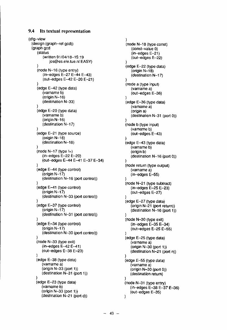
9.4 Its textual representation

(dfg-view (design (graph-ref gcd)) (graph gcd

(status

)

(written 91/04/18-15:19 [email protected] EASY)

(node N-16 (type entry) (in-edges E-27 E-44 E-43) (out-ildges E-42 E-20 E-21)

) (edge E-42 (type data)

(varname b)

)

(origin N-16) (destination N-33)

(edge E-20 (type data) (varname b)

)


(edge E-21 (type source) (origin N-16) (destination N-18)

) (node N-17 (type ,=)

(in-edges E-22 E-20) (out-edges E-44 E-41 E-37 E-34)

) (edge E-44 (type control)

(origin N-17) (destination N-16 (port control))







) (node N-33 (type exit)

(in--ildges E-42 E-41) (out-edges E-38 E-23)


(varname a)

)

(origin N-33 (port 1)) (destination N-31 (port 1))

(edge E-23 (type data) (varname b) (origin N-33 (port 1)) (destination N-21 (port d))

- 43 -

) (node N-18 (type const)

(const-value 0) (in-edges E-21) (out-ildges E-22)



) (node a (type input)

(varname a) (out-ildges E-36)


(varname a) (origin a) (destination N-31 (port 0))

) (node b (type input)

(varname b) (out-ildges E-43)


(varname b) (origin b) (destination N-16 (port 0))

) (node return (type output)

(varname a) (in-edges E-55)

) (node N-21 (type subtract)

(in-edges E-25 E-23) (out-ildges E-27)


(origin N-21 (port return)) (destination N-16 (port 1))


(in-edges E-35 E-34) (out-edges E-25 E-55)


(varname a)

)

(origin N-30 (port 1)) (destination N-21 (port n))

(edge E-55 (type data) (varname a)

)

(origin N-30 (port 0)) (destination return)

(node N-31 (type entry) (in-edges E-38 E-37 E-36) (out-ildges E-35)

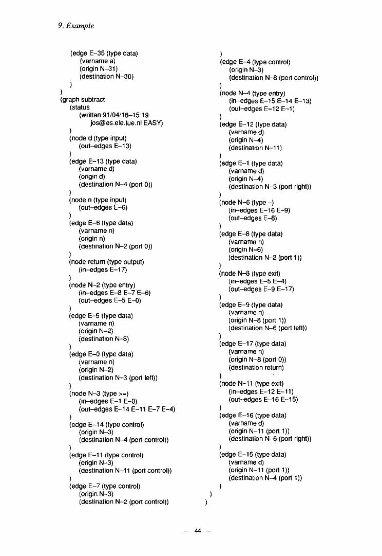
9. Example

)

(edge E-35 (type data) (varname a) (origin N-31) (destination N-30)

(graph subtract (status

)

(written 91/04/18-15:19 [email protected] EASY)

(node d (type input) (out-edges E-13)


(varname d) (origin d) (destination N-4 (port 0))

) (node n (type input)

(out-edges E-6) ) (edge E-6 (type data)

(varname n) (origin n) (destination N-2 (port 0))

) (node retum (type output)

(in-edges E-17) ) (node N-2 (type entry)

(in-edges E-8 E-7 E-6) (out-edges E-5 E--{))


(varname n) (origin N-2) (destination N-8)

) (edge E--{) (type data)

(varname n) (origin N-2) (destination N-3 (port left))

) (node N-3 (type >=)

(in-edges E-1 E-O) (out-edges E-14 E-11 E-7 E-4)



) (edge E-l1 (type control)




) )

- 44 -



) (node N-4 (type entry)

(in-edges E-15 E-14 E-13) (out-edges E-12 E-1)


(varname d)

)


(edge E-1 (type data) (varname d) (origin N-4) (destination N-3 (port right))

) (node N-6 (type -)

(in-edges E-16 E-9) (out-edges E-8)


(varname n) (origin N-6) (destination N-2 (port 1))


(in-edges E-5 E-4) (out-edges E-9 E-17)


(varna me n)

)

(origin N-8 (port 1)) (destination N-6 (port left))

(edge E-17 (type data) (varname n)

)

(origin N-8 (port 0)) (destination return)

(node N-11 (type exit) (in-edges E-12 E-11) (out-edges E-16 E-15)


(varname d)

)

(origin N-11 (port 1)) (destination N-6 (port right))

(edge E-15 (type data) (varname d) (origin N-l1 (port 1)) (destination N-4 (port 1))

10. Epilogue

This release of the manual described two important extensions to the DFG standard: data types and parameterization. We believe that we succeeded in developing well defined and general concepts for these, which can easily be extended maintaining both upwards and downwards compatibility. Smaller extensions were the introduction of multidimensional arrays, and a 'delay' node. These extensions should serve the most direct needs. Of course such discussions should be continued to maintain satisfactory cooperation in the future.

Compared with the previous manual, the text was extended and refined at many points. Furthermore several figures were added to clarify the intentions. This effort will hopefully help in a better understanding and acceptance of the standard.

We strongly believe that our ASCIS data flow graph exchange format has several unsurpassed qualities which make it worldwide unique. It is now to the project partners to !,'Tab this advantage and make it a benefit for the project as a whole.

Jos van 'EijntffuJ1Jen

Leon Stat

(jjalt de Jong

- 45 -

1l.lndex

11. Index

A E integer, 14, 15 interfaces, I

array, II, 12,28,33,37 edge ascii,25 chain, 10, 11, 18, 33, 34

K ASCIS, 1,45 control, 6, 32, 34 data, 34 keyword, 25, 26 property, 14

B semantics, 4 source, 5, 18, 33, 35 L

bit fields, 14 timing, 18, 35

bit pattern, 14, 15, 18,39 type,29,34,37,40 lexical analysis, 25

bitvector, 23 width,17 library, 21

boolean, 6, 14, 16 ELLA,I loop construct, 7

bounding box, 40 error message, 30

braces, 25 evaluation, order of, 4 M execution, 4, 5, 9, 10, 12

exponent, 16 multirate, 10 expression, 36, 37

C extension, 25, 39 external world, 10 N case, 25

case-{)f,7 node clock, 9, 20, 37 F array, II, 12,33 comment bit operations, 31

statement, 25, 27 file, 14,29 branch, 6, 32 string, 26 fixed point, 16 constant, 5

communication, 10 for-do,7 control,32 complexity, 3 format, I, 25 delay, 12,33 constant, 11, 15, 18,26,28, entry, 7,32

33,35,37

G exit, 7,32

cycle, 8, 12, 41 get, 10,33

goals, I input, 5, 10, 33

graph, execution, 5 merge, 6, 32

D graph name, 35 noop, 33 numeric operations, 30

data flow graph, I operation, 4, 39 data type, 14,26,27,29,37 H output, 5, 10, 33

boolean, 16 position, 40 fixed point, 16 hardware, 12, 14 predefined types, 30 integer, 15 Hardware C, 1,41 put, 10,33

data width, 14 hierarchy, 29, 35 retrieve, 11, 34 decimal number, 15 semantics, 4 delay, 20, 35, 37 type, 4, 30, 40

maximum, 29 I type name, 5 minimum, 29 update, II, 34 ripple, 23, 29 identifier, 26, 36 number, 26 specification, 21 if-then--else, 7,32 decimal,26

delimiter, 25 initialization, 9, 12 hexadecimal, 26 design, 29 instantiation, 5, 12,22,29, octal,26 drawing, 40 33, 35 numeric, 15

- 46 -

0 S queue,4,33 timing, 23

operation, 4, 30 selection list, 6, 9, 37 tools, 2,40 optimization, 2, 41 semantics, 4, 20 two--complement, 16 ordering, 11 semicolon, 26

signed magnitude, 16

p Silage, 1 U simulation, 12, 14 source, 5 unfolding, 9

pad,lO state, 12 unsigned, 16 parameter subgraph,5

assignment, 36 support, 40 data type, 36 syntax, 25, 27 V declaration, 36 synthesis, 1, 20 default value, 37

verification, 1, 40 parameterization, 36 parser, 25, 41 T VHDL,1

parsing, 2 port, 4 text, 25

control,6 time, 12,20 W name, 5, 40 asynchronous,20,37 physical, 10 constraint, 20 while-<io, 7

width, 17 interval, 20, 29, 37 white space, 25

postscript, 40 max constraint, 29 width, 14, 17,29,37

procedure, 5, 10, 12 min con straint, 29 adjustment, 17 model,22 default, 14 synchronous, 20, 37

R violation, 22 timing, 9, 35 X records, 14 token, 4

references, 1, 4 multiple, 4, 10 X window, 40

- 47 -

ISSN 0167-9708 Coden: TEUEDE

(222) Jozwiak, L. THE FuLL-DECOMPOSITION OF SEQUENTIAL MACHINES WITH THE SEPARATE REALIZATION OF THE NEXT-STATE AND OUTPUT FUNCTIONS. EUT Report 89-E-222. 1989. ISBN 90-6144-222-2

(223) Jozwiak, L. THE BIT FULL-DECOMPOSITION OF SEQUENTIAL MACHINES. EUT Report 89-E-223. 1989. ISBN 90-6144-223-0

(224) Book of abstracts of the first Benelux-Japan Workshop on Information and Communication Theory, Eindhoven, The Netherlands, 3-5 September 1989.

(225)

(226)

Ed. by Han Vinck. EUT Report ~224. 1989. ISBN 90-6144-224-9

Hoei~makers, M.J. A PO SIBILITY TO INCORPORATE SATURATION IN THE SIMPLE, OF A SYNCHRONOUS MACHINE WITH RECTIFIER. EUT Report 89-E-225. 1989. ISBN 90-6144-225-7

GLOBAL MODEL

~ahkAi' R.P. and E.M. van Veldhuizen, W.R. R~~~~~nL.H.Th. Rietj'ens XP MENTS ON INITIAL BEHAVIoUR OF CORONA? WITH ELECTR CAL

PULSES SUPERIMPOSED ON DC BIAS. EUT Report 89-E-226. 1989. ISBN 90-6144-226-5

(227) Bastings, R.H.A. TowARD THE DEVELOPMENT OF AN INTELLIGENT ALARM SYSTEM IN ANESTHESIA. EUT Report 89-E-227. 1989. ISBN 90-6144-227-3

(228) Hekker, J.J. ~ER ANIMATED GRAPHICS AS A TEACHING TODL FOR THE ANESTHESIA MACHINE SIMULATOR. EUT Report 89-E-228. 1989. ISBN 90-6144-228-1

(229) Oostroffi, J.H.M. van iNTELLIGENT ALARMS IN ANESTHESIA: An implementation. EUT Report 89-E-229. 1989. ISBN 90-6144-229-X

(230) Winter, M.R.M. ~ OF A UNIVERSAL PROTOCOL SUBSYSTEM ARCHITECTURE: Specification of functions and services. EUT Report 89-E-230. 1989. ISBN 90-6144-230-3

(231) Schemmann, M.F.C. and H.C. Heyker, J.J.M. Kwaspen, Th.G. van de Roer MOUNT I NG AND DC TO 18 GHz CHARACTER I SA TI ON OF DOUBLE BARR I ER RESONANT TUNNELING DEVICES. EUT Report 89-E-231. 1989. ISBN 90-6144-231-1

(232) Sarma, A.D. and M.H.A.J. Herben IlATAACQUI S IT I ON AND SIGi;iiL1'ROCESS I NG/ANALYS I S OF SC I NTI LLAT I ON EVEIHS FOR THE OLYMPUS PROPAGATION EXPER I MENT. EUT Report 89-E-232. 1989. ISBN 90-6144-232-X

(233) Nederstigt, J.A.

(234)

DESIGN AND IMPLEMENTATION OF A SECOND PROTOTYPE OF THE INTELLIGENT ALARM SYSTEM IN ANESTHESIA. EUT Report 90-E-233. 1990. ISBN 90-6144-233-8

Phili~TensJ E.H.J. DESIG NG DEBUGGING TOOLS FOR SIMPLEXYs EXPERT SYSTEMS. EUT Report 90-E-234. 1990. ISBN 90-6144-234-6

(235) Heffels, J.J.M.

(236)

A PATIENT SIMULATOR FOR Ar~ESTHESIA TRAINING: A mechanical lung model and a physiological software model. EUT Report 90-E-235. 1990. IS8N 90-6144-235-4

J.O. BASED ADAPTIVE BLOOD PRESSURE CONTROL: A Simplexys expert system

application. EUT Report 90-E-236. 1990. ISBN 90-6144-236-2

(237) Ren Qingchang ~DICTION ERROR METHOD FOR IDENTIFICATION OF A HEAT EXCHANGER. EUT Report 90-E-237. 1990. ISBN 90-6144-237-0

Eindhoven University of Technology Research Reports Faculty of Electrical Engineering

I SSI' 0167-9708 Coden: TEUEDE

(238) Lammers, J.D. [HE USE OF PETRI NET THEORY FOR SIMPLEXYS EXPERT SYSTEMS PROTOCOL CHECKING. EUT Report 90-E-238. 1990. ISBN 90-6144-238-9

(239) WRE9J X. P LlMINARY INVESTIGATIONS ON TACTILE PERCEPT/Qt, OF GRAPHICAL PATTERNS. EUT Report 9Q-E-239. 1990. ISBN 90-6144-239-7

(240) Lutgens, J.M.A. KNOWLEDGE BASE CORRECTNESS CHECKING FOR SIMPLEXYS EXPERT SYSTEMS. EUT Eeport 90-E-240. 1990. ISBN 90-6144-240-0

(241) Brinker, A.C. den A MEMBRANE MODEL FOR SPATIDTEMPORAL CDUPLING. EUT Report 9D-E-241. 1990. ISBN 90-6144-241-9

(242)

(243)

J.J.M. and H.C. ~tSkON' J.I.M. Demartea~, Th.G. van de Roer NDISE MEASUREME DOUBLE BARRIER RESONANT TUNNELIN~DDES.

EUT Report 90-E-242. 1990. ISBN 90-6144-242-7

Massee, P. and H.A.L.M. de Graaf, W.J.M. Balemans, H.G. Knoopers, H.H.J. ten Kate --PREDrsTCN OF AN EXPERIMENTAL (5-10 MWt) DISK MHD FACILITY AND PROSPECTS OF COMMERCIAL (1000 MWt) MHD/STEAM SYSTEMS. EUT Report 90-E-243. 1990. ISBN 90-6144-243-S

(244) Klompstra, Martin and Ton van den Boom, Ad Damen A COMPARISON OF CLASSICAL AND MODEnNrCoNTROIII]'DESIGN: A case study. EUT Report 90-E-244. 1990. ISBN 90-6144-244-3

(245) ~r~, P.H.G. van de HE ACCURACY OF RADIOWAVE PROPAGATION MEASUREMENTS: Olympus propagation

experiment. EUT Report 90-E-245. 1990. ISBN 90-6144-245-1

(246) ~asg~, P.J.L. de Y THESIS METHOD FOR COMBINED OPTIMIZATION OF MULTIPLE ANTENNA PARAMETERS

AND ANTENNA PATTERN STRUCTURE. EUT Report 90-E-246. 1990. ISBN 90-6144-246-X

(247) Jozwiak, L. and T. s~assova-Kwaaitaal ~OSITIONAL STAT ASSiGNMENT WiTH REUSE OF STANDARD DESIGNS: Using counters as sub-machines and using the method of maximal adjacensies to select the state chains and the state codes.

(248)

(249)

(2S0)

(251 )

EUT Report 90-E-247. 1990. ISBN 90-6144-247-8

Hoeijmakers, M.J. and J.M. Vleeshouwers DERIVATION AND VERIFICATION OF A MODEL OF THE SYNCHRONOUS MACHINE WITH RECTIFIER WITH TWO DAMPER WINDINGS ON THE DIRECT AXiS. EUT Report 90-E-248. 1990. ISBN 90-6144-248-6

Zhu, V.C. and A.C.P.M. Backx, P. Eijkhoff MULTIVARIABLE PROCESS 15rNTlFICATI N FOR ROBUST CONTROL. EUT Report 91-E-249. 1991. ISBN 90-6144-249-4

Pfaffenhofer, F.M. and P.J.M. Cluitmans, H.M. Kuipers EMDABS: Design and formal specification of a datamodel research database system. EUT Report 91-E-250. 1991. ISBN 90-6144-250-8

for a clinical

Eitndhoven, J.T.J. van and C.C. de Jon9, L. Stok TH ASCIS DATA FLOW GRAPH: Semantics and textual format. EUT Report 91-E-2S1. 1991. ISBN 90-6144-251-6

the ascis data flow graph : semantics and textual format

Documents