the application of gis and rs for coastline change ......using rs and gis. the change detection...
TRANSCRIPT
The Application of GIS and RS for Coastline Change Detection and Risk Assessment to Enhanced Sea Level Rise
Yellow River delta, China
by Tang Yanli
Thesis submitted to International Institute for Geoinformation Science and Earth Observation in par-tial fulfilment of the requirements for the degree in Master of Science in Natural Hazard Studys. Degree Assessment Board Thesis examiners Dr. N. Rengers (Chairman), ITC Dr. S.W.M. Peters (External Examiner), Vrije University. Amsterdam Drs. M.C.J.Damen (First supervisor) Dr. B.H.P. Maathuis (Second supervisor) Dr. Tjeerd Willem Hobma Drs. N.C. Kingma
INTERNATIONAL INSTITUTE FOR GEOINFORMATION SCIENCE AND EARTH OBSERVATION
ENSCHEDE, THE NETHERLANDS

II
Disclaimer This document describes work undertaken as part of a programme of study at the International Institute for Aerospace Survey and Earth Sciences. All views and opinions expressed therein remain the sole responsibility of the author, and do not necessarily represent those of the insti-tute.
III
ABSTRACT The active part of the Yellow River Delta (YRD) is one of the most rapid expanding deltas in the world. It is experiencing relatively strong environmental changes resulting from the complex interac-tion of natural and human-induced processes that operate upon it. The research focuses on the Yellow River Delta coastline change detection and risk assessment to enhanced sea level rise and storm surge using RS and GIS. The change detection involves, processing of multi-temporal images (1992-2001), followed by image differencing, post-classification image overlaying, image fusion, image visual interpretation and on-screen digitising. The result shows that the image differencing and post-classification image overlay-ing change detection techniques are useful to monitor coastline change. The image visual interpreta-tion and on-screen digitising was the main quantitative method to detect the Yellow River Delta coast-line change. Quantitative measurement and analysis show that the delta area and the Yellow River channel length tend to increase in past ten years. The natural factors and human activities played an important role on the Yellow River Delta development. The risk assessment included the prediction of social-economic factors, the storm surge flood model-ling, and the vulnerability analysis, damage and risk assessment. An estimated relative sea level rise of 48cm by 2050, and 88cm by 2100 were considered in the study. The result shows that the Yellow River Delta will suffer from critical flood damage as a result of enhanced sea level rise and storm surge. Keywords: the Yellow River Delta, GIS, RS, Coastline change detection, Risk assessment, Sea level rise.

IV
ACKNOWLEDGEMENTS I would like to express my sincere gratitude to the Netherlands Fellowship Program (NFP) for provid-ing financial support to pursue this higher level of education in ITC and hugely improving the confi-dence level in my profession. My special thanks also go to the China State Bureau of Surveying and Mapping, and Heilongjiang Bureau of Surveying and Mapping, for allowing me to study abroad. I am greatly indebted to Drs Michiel C.J. Damen and Dr. B.H.P. Maathius my supervisors. Their guidance, invaluable suggestions and critical reading of the manuscript have contributed to the quality of this dissertation. My sincere thanks go to Dr. Cees Van Western, the students’ adviser for his guidance and assistance during my entire stay in the Netherlands. I also thank Dr. T.W. Hobma, Drs. Kingma, QingLian Tian, and Dr. P.G.V Voskuil for the discussions in their special fields. Special thanks also go to Drs Boudewijn de Smith and Dr. Van dijk for their immense support in the extension from PM to MSc. degree course. I thank my fellow Chinese students ZhangLei, Wang Xiaoping, Wang Chunging and Hudeibin. Spe-cial thanks to other fellow students Winwin ambarwulan, Mamay Surmayadi, Heri Sutanta (all from Indonesia), Elena (Costa Rica), Urban German, (Mexico), Edgar Lanz (Mexico), Juan (Colombia), Forson Karikari (Ghana), Lucas Donny Setijadji (Indonesia) Jesus Moreira (Cuba) and Gilbert Mhlanga (Zimbabwe) for their companionship and assistance during the period of study. My heartfelt gratitude goes to my parents Mr. Tangguofan and Mrs. Chengshuqin for looking after my family in my absence. I am most appreciative of the understanding, love, support of my husband Liwen and son Lipenyu. If this has been an achievement, it is for you, as you are the people who have sacrificed and suffered most. Above all, I thank Prof. J.L. Van Genderen, for his special role in helping me to study in ITC.

V
TABLE OF CONTENTS
ABSTRACT......................................................................................................................................................... III
ACKNOWLEDGEMENTS ................................................................................................................................. IV
LIST OF FIGURE............................................................................................................................................. VIII
LIST OF TABLES................................................................................................................................................ X
LIST OF TABLES................................................................................................................................................ X
1. INTRODUCTION ......................................................................................................................... 1
1.1. BACKGROUND ........................................................................................................................ 1 1.2. DEFINITION OF THE PROBLEM ................................................................................................ 1 1.3. RESEARCH QUESTION............................................................................................................. 2 1.4. RESEARCH OBJECTIVES ......................................................................................................... 2
1.4.1. Change detection of Yellow River Delta coastline ....................................................... 2 1.4.2. Risk assessment to sea level rise relative storm surge................................................... 2
1.5. HYPOTHESIS AND ASSUMPTIONS ........................................................................................... 3 1.6. PREVIOUS REVIEW ................................................................................................................. 3
2. METHODOLOGY ........................................................................................................................ 7
2.1. METHODOLOGY ..................................................................................................................... 7 2.1.1. Data collection............................................................................................................... 7 2.1.2. Coastline change detection of active YRD.................................................................... 7 2.1.3. Assessment of coastal risk to sea level rise-related storm surge ................................... 7
2.2. MATERIALS USED .................................................................................................................. 8 2.2.1. Available Data ............................................................................................................... 8 2.2.2. Software......................................................................................................................... 9
2.3. FLOWCHART OF METHODOLOGY .......................................................................................... 11 2.3.1. Yellow River Delta coastline change detection........................................................... 11 2.3.2. Risk Assessment to sea level rise-related storm surge ................................................ 11
3. DESCRIPTION OF THE STUDY AREA .................................................................................. 13
3.1. DESCRIPTION OF THE YELLOW RIVER DELTA ..................................................................... 13 3.1.1. Location and general geographic background............................................................. 13 3.1.2. Discharge of the Yellow River .................................................................................... 13 3.1.3. Migration of the main channel..................................................................................... 16 3.1.4. Formation of the Delta................................................................................................. 16 3.1.5. Coastline chnage.......................................................................................................... 18
3.2. HYDRAULIC SETTING OF THE BOHAI SEA ........................................................................... 19 3.2.1. General Topographic Features .................................................................................... 19 3.2.2. Tides and Currents....................................................................................................... 19 3.2.3. Wind and Storm Surge................................................................................................. 20
VI
3.2.4. Wind Wave .................................................................................................................. 21 3.2.5. Residual Currents ........................................................................................................ 21
3.3. SEA LEVEL RISE AND LAND SUBSIDENCE ........................................................................... 21 3.3.1. Sea Level Rise ............................................................................................................. 21 3.3.2. Land Subsidence.......................................................................................................... 22
4. COASTLINE CHANGE DETECTION ...................................................................................... 23
4.1. IMAGE PROCESSING ............................................................................................................. 23 4.1.1. Landsat and Aster image processing ........................................................................... 23 4.1.2. ERS1/2 image processing ............................................................................................ 24
4.2. IMAGE CLASSIFICATION FOR CHANGE DETECTION............................................................... 28 4.2.1. Image classification ..................................................................................................... 28 4.2.2. Change detection ......................................................................................................... 28
4.3. IMAGE INTERPRETATION AND ANALYSIS FOR CHANGE DETECTION..................................... 35 4.3.1. Optical images interpretation and coastline change analysis ...................................... 36 4.3.2. Radar image interpretation and comparison of results ................................................ 40
4.4. CONCLUSION AND DISCUSSIONS .......................................................................................... 42 4.4.1. The impacts of the fluvial process............................................................................... 42 4.4.2. The impacts of the marine processes........................................................................... 43 4.4.3. Human activities .......................................................................................................... 44
5. VULNERABILITY ASSESSMENT OF THE YRD TO SEA LEVEL RISE-RELATED STORM SURGE ................................................................................................................................................ 46
5.1. CONCEPTUAL FRAMEWORK ................................................................................................. 46 5.1.1. Conceptual framework of vulnerability assessment to sea level rise.......................... 46 5.1.2. Conceptual framework of risk assessment of natural hazard ...................................... 48 5.1.3. Risk assessment of the YRD to SLR related storm surge ........................................... 49
5.2. CREATION OF DATABASE..................................................................................................... 49 5.2.1. Creation of a digital elevation model .......................................................................... 49 5.2.2. Prediction of socio-economic factors and flood estimates .......................................... 50 5.2.3. Generation of thematic maps....................................................................................... 52
5.3. MODELLING OF STORM FLOODING TO SEA LEVEL RISE........................................................ 54 5.3.1. Storm Surge Flood modelling...................................................................................... 56
5.4. VULNERABILITY ASSESSMENT TO SOCIAL-ECONOMIC RISK ELEMENTS .............................. 57 5.5. DAMAGE AND LOSS ASSESSMENT ........................................................................................ 60
5.5.1. Casualties and loss of GDP assessment....................................................................... 60 5.5.2. Assessment of the losses of urban and agriculture...................................................... 60 5.5.3. Assessment of the loss of natural reserve and tidal flat area....................................... 61
5.6. RISK ASSESSMENT................................................................................................................ 62 5.6.1. Risk zonation mapping for population and GDP......................................................... 62 5.6.2. Overall annual risk for landuse.................................................................................... 64
5.7. CONCLUSION........................................................................................................................ 66
6. CONCLUSION AND RECOMMENDATION........................................................................... 68
6.1. CONCLUSION AND RECOMMENDATION FOR COASTLINE CHANGE DETECTION..................... 68

VII
6.1.1. Conclusion ................................................................................................................... 68 6.1.2. Recommendation ......................................................................................................... 69
6.2. CONCLUSION AND RECOMMENDATION FOR RISK ASSESSMENT........................................... 69 6.2.1. Conclusion for risk assessment.................................................................................... 69 6.2.2. Recommendation ......................................................................................................... 69

VIII
LIST OF FIGURE Fig. 2.1 Synoptic flowchart of methodology to Change Detection of yellow river Delta coastline
change.......................................................................................................................................... 11 Fig 2.2 Flowchart of Risk Assessment to sea level rise-related storm surge...................................... 12 Fig.3.1 Study Area............................................................................................................................... 14 Fig.3.2 Water discharge....................................................................................................................... 16 Fig.3.3 Shifting of distributary channels, depositional deltaic Lobes of the modern Yellow River Delta
..................................................................................................................................................... 17 Fig.3.4 Coastline change in the modern Yellow River Delta 1855-1989 ........................................... 18 Fig.3.5 Submarine topographic map of the Bohai Sea........................................................................ 19 Fig.3.6 M2 partial tidal wave system in the Bohai Sea....................................................................... 20 Fig. 3.7 The estimated Global Sea Level Rise .................................................................................... 22 Fig.4.1 the procedures of radiometric correction. ............................................................................... 25 Fig.4.3 The SAR image after (a) and before (b) speckle-reduction (ERS2 image, Dec.22, 1999)..... 26 Fig4.2 Flowchart of ERS1/2 image processing................................................................................... 27 Fig.4.4 The histogram of image ytm94b5 Fig. 4.5 The histogram of image ytm00b5 ..... 29 Fig 4.6 The classification map of ytm94b5 Fig. 4.7 The classification map of ytm00b5 .... 29 Fig 4.8 Change detection through image differencing........................................................................ 32 Fig.4.9 change detection through crossing two classified images ...................................................... 33 Fig. 4.10 Image fusion Aster01 b2, ERS92, Aster01 b1 (RGB) ......................................................... 34 Fig.4.11 Image fusion ytm00b4,b5,ers96 (RGB)................................................................................ 34 Fig. 4.12 the tidal flat on Landsat image 1992 (FCC)......................................................................... 37 Fig. 4.13 The mask of study area for coastline change detection on the Landsat image (May.2 2000)38 Fig. 4.14 The development of the most active delta on optic image interpretation............................ 38 Fig 4.15 Curve of the YRD area change Fig 4.16 Curve of YRD area change characteristic
..................................................................................................................................................... 40 Fig 4.17 The curves of coastline shift from the position of 1992 along 5 profiles ............................ 40 Fig. 4.18 The development of the most active delta from Radar image interpretation ...................... 41 Fig. 4.19 Linear fit of coastline shift between ERS and Landsat images ........................................... 42 Fig 4.20 The comparison of the deltaic area against river channel length.......................................... 43 Fig.4.21 Correlation between dry out days and delta area .................................................................. 43 Fig. 4.22 Most active Yellow River Delta on Radar image (Dec. 11,1999) ....................................... 45 Fig 5.1 Seven steps for the assessment of the vulnerability of coastal area to seal level rise ............ 47 Fig.5.2 Flow chart for the creation of DEM........................................................................................ 50 Fig.5.3.DEM map of the YRD ............................................................................................................ 50 Fig5.4 The prediction of population increasing rate ........................................................................... 51 Fig.5.5 the flowchart of creation of administrative map..................................................................... 52 Fig5.6 flowchart of the procedure to make the landuse development map in ILWIS ........................ 55 Fig.5.7 Flood depth map for 50 storm surge return periods with SLR of 48 cm................................ 57 Fig5.8 relation vulnerability and flood depth for pop Fig5.9 relation vulnerability and flood depth for
GDP ............................................................................................................................................. 58 Fig.5.10 Relation vulnerability and flood depth for urban Fig. 5.11 Vulnerability for agriculture. 58

IX
Fig. 5.16 Risk map of POP for 50 RP without SLR Fig. 5.17 Risk map of POP for 50 RP with SLR 48 cm ........................................................................................................................................... 64
Fig. 5.18 Risk map of POP for 100 RP with SLR 48cm Fig. 5.19 Risk map of GDP for 50 RP without SLR.............................................................................................................................................. 64
Fig. 5.20 Risk map of GDP for 50 RP with SLR 48 cm Fig. 5.21 Risk map of GDP for 100 RP with SLR 48 cm................................................................................................................................... 64
Fig.5.22 Loss probability curve without SLR Fig.5.23 Loss probability curve with SLR 48cm 65 Fig.5.24 Loss probability curve with SLR 88cm ................................................................................ 65

X
LIST OF TABLES
Table2.1 The water level to sea level rise combined with Storm Surge ............................................... 8 Table 2.2 Characteristics of the used image data .................................................................................. 9 Table 2.3 Sensor characteristics .......................................................................................................... 10 Table3.1 Hydrologic Characteristics of Some of the World’s Major Rivers ...................................... 15 Table 3.2 hydrologic data collection at Lijing Station during the period 1976-1985......................... 15 Table 3.3 Relative sea level changes at station in the Yellow River delta.......................................... 22 Table 4.1 Statistics about the result of radiometric correction ........................................................... 25 Table 4.2 ERS image geometric correction and registration .............................................................. 26 Table 4.3 Overview of change detection technique ............................................................................ 31 Table 4.4 an output of change detection image through image-differencing operation ..................... 32 Table 4.5 The cross table of post-classification maps (ytm94b5c and ytm00b5c) ............................. 33 Table 4.6 Tidal conditions of the images ............................................................................................ 37 Table 4.8 Characteristics of deltaic coastline shift Table 4.9 Deltaic area changing .............. 37 Table 4.10 The distance comparison of coastline shift between ERS (lower tidal level) and Landsat
images (high tidal level) .............................................................................................................. 41 Table 4.11days of dry out of the Yellow River and its length ............................................................ 43 Table 5.1 statistic data of PIR and GIP from 1985 to 1999 ................................................................ 51 Table 5.2 the extension prediction of urban area by 2050 and 2100 .................................................. 52 Table 5.4 Calculation of population and GDP density........................................................................ 53 Table 5.5 the monetary value of elements at risk................................................................................ 54 Table 5.6 the storm surge levels predicted by 2050 and 2100 for each return period ........................ 56 Table 5.7 Flood depth and respective Vulnerability coefficient ......................................................... 58 Table 5.8 the number of casualties and GDP loss for each flooding scenario.................................... 60 Table 5.9 the losses of urban and agriculture for each flooding scenario (million in RMB) ............. 61 Table 5.10 the lost area of the natural reserve and tidal flat for 48 cm and 88 cm SLR scenario ...... 61 Table 5.11 the effected area of the natural reserve and tidal flat for each flooding scenario ............. 61 Table 5.12 The calculation of overall risk without SLR ..................................................................... 65 Table 5.13 The calculation of overall risk with SLR 48cm ................................................................ 66 Table 5.14 The calculation of overall risk with SLR 88cm ................................................................ 66
Yellow River Delta Change Detection and Risk Assessment to Sea Level Rise
1
1. INTRODUCTION
1.1. Background
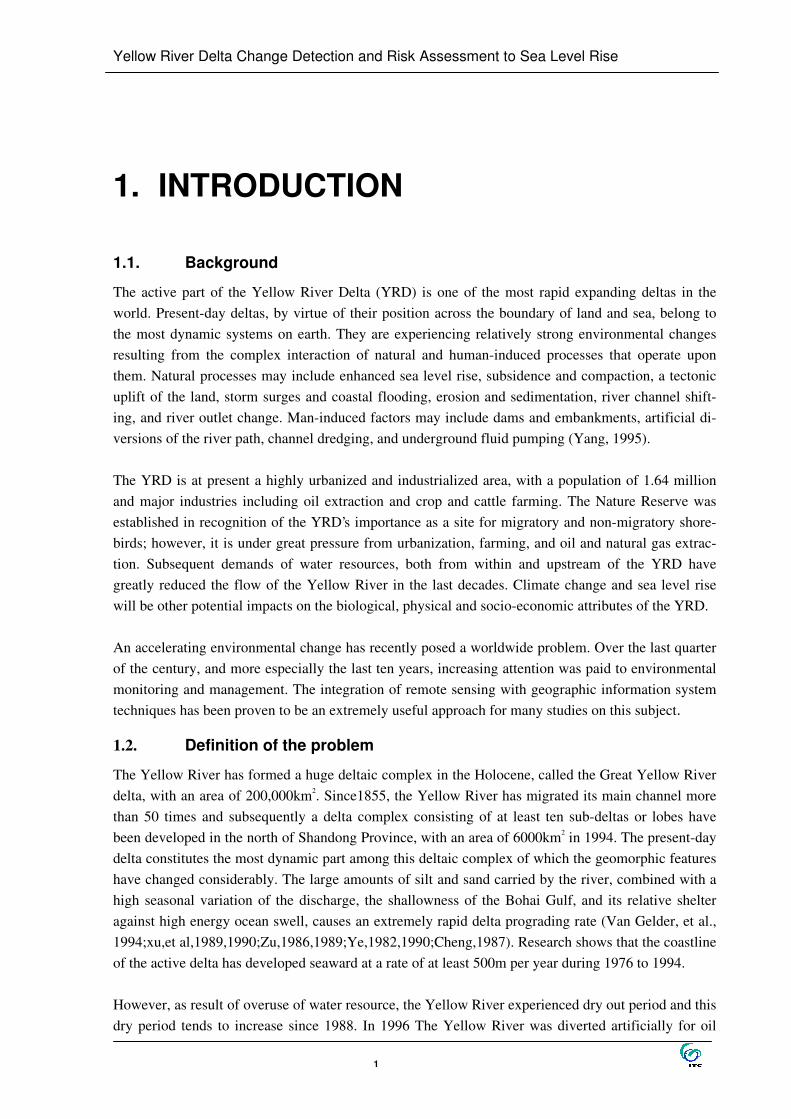
The active part of the Yellow River Delta (YRD) is one of the most rapid expanding deltas in the world. Present-day deltas, by virtue of their position across the boundary of land and sea, belong to the most dynamic systems on earth. They are experiencing relatively strong environmental changes resulting from the complex interaction of natural and human-induced processes that operate upon them. Natural processes may include enhanced sea level rise, subsidence and compaction, a tectonic uplift of the land, storm surges and coastal flooding, erosion and sedimentation, river channel shift-ing, and river outlet change. Man-induced factors may include dams and embankments, artificial di-versions of the river path, channel dredging, and underground fluid pumping (Yang, 1995). The YRD is at present a highly urbanized and industrialized area, with a population of 1.64 million and major industries including oil extraction and crop and cattle farming. The Nature Reserve was established in recognition of the YRD’s importance as a site for migratory and non-migratory shore-birds; however, it is under great pressure from urbanization, farming, and oil and natural gas extrac-tion. Subsequent demands of water resources, both from within and upstream of the YRD have greatly reduced the flow of the Yellow River in the last decades. Climate change and sea level rise will be other potential impacts on the biological, physical and socio-economic attributes of the YRD. An accelerating environmental change has recently posed a worldwide problem. Over the last quarter of the century, and more especially the last ten years, increasing attention was paid to environmental monitoring and management. The integration of remote sensing with geographic information system techniques has been proven to be an extremely useful approach for many studies on this subject.
1.2. Definition of the problem
The Yellow River has formed a huge deltaic complex in the Holocene, called the Great Yellow River delta, with an area of 200,000km2. Since1855, the Yellow River has migrated its main channel more than 50 times and subsequently a delta complex consisting of at least ten sub-deltas or lobes have been developed in the north of Shandong Province, with an area of 6000km2 in 1994. The present-day delta constitutes the most dynamic part among this deltaic complex of which the geomorphic features have changed considerably. The large amounts of silt and sand carried by the river, combined with a high seasonal variation of the discharge, the shallowness of the Bohai Gulf, and its relative shelter against high energy ocean swell, causes an extremely rapid delta prograding rate (Van Gelder, et al., 1994;xu,et al,1989,1990;Zu,1986,1989;Ye,1982,1990;Cheng,1987). Research shows that the coastline of the active delta has developed seaward at a rate of at least 500m per year during 1976 to 1994. However, as result of overuse of water resource, the Yellow River experienced dry out period and this dry period tends to increase since 1988. In 1996 The Yellow River was diverted artificially for oil

Yellow River Delta Change Detection and Risk Assessment to Sea Level Rise
2
extraction purpose. Further China government has succeeded in the Yellow River water management project since 1999. This reduces time of no discharge of the Yellow River. Above all factors have the important impact on the YRD‘s change. The climate change and sea level rise are a global problem. According to a project entitled "Vulner-ability Assessment of Major Wetlands in the Asia-Pacific Region", the estimated relative sea level rise rate in the Yellow River Delta is 8 mm/year and the sea level rise will be 48 cm by the year 2050. (http://www.ea.gov.au/ssd/publications/ ssr/149.html). This will lead to critical impacts such as the frequency of storm surges. The sea level rise aggravates the flood disaster resulting from storm surge. Although the sea level rise is a slow process, it should be regarded and taken precaution as a key fac-tor to the sustainable development of the YRD for its extensive influence. Due to effect of sea level rise relative to storm surge, The YRD will face a serious flood problem.
1.3. Research question
How did YRD coastline change in the past decade (from 1992 to 2001)? What role did the natural factors and human activities play on the changing of the YRD? How much damage will be the result from enhanced sea level rise relative to storm surge? Application of GIS and RS technology provides an advantage to answer those questions.
1.4. Research Objectives
The objectives of this study can be divided into two sub-objectives: firstly to detect the coastline change of active YRD using multiple space-borne remote sensing sources; secondly to assess coastal flood damage and risk resulting from enhanced sea level rise using the integrated approach of RS and GIS. To accomplish the two main objectives of research, the following tasks will be carried out:
1.4.1. Change detection of Yellow River Delta coastline
• Detection and identifying of the coastline change in the sub-delta since 1992 using different approaches;
• Analysis of the reasons of coastline change; • Evaluation of satellite remote sensed data as an input for the detection of coastline change,
and the assessment of digital image processing and GIS techniques for the quantification of coastline change.
1.4.2. Risk assessment to sea level rise relative storm surge
• Prediction of socio-economic development of the YRD by 2050 and 2100 • The modelling of sea level rise hazard in combination with storm surge height. • Assessment of damage and risk on socio-economic factors to sae level rise and storm surge
by 2050 and 2100 • The analysis of effect of sea level rise
Yellow River Delta Change Detection and Risk Assessment to Sea Level Rise
3
1.5. Hypothesis and Assumptions
The relative sea level rise rate in the Yellow River Delta is 8 mm/year; consequently the sea level rise will be 48cm by the year 2050, and 88cm by the year 2100 (based on the elevation of 1999).
1.6. Previous review
As the most dynamic delta on earth, Yellow River Delta received a lot of attention. Many papers and theses of YRD change detection were published. ITC thesis titled “Monitoring morphodynamic as-pects of the present Huanghe River (Yellow River) Delta, China, an approach of the integration of satellite remote sensing and geoinformatic system (GIS)” by Yang Xiaojun, applied an integrated ap-proach of RS and GIS for the monitoring and detection of the morphological changes of the present Yellow River Delta. The Landsat MSS and TM images covering 19 years (1976-1994) are the main source of data. This study emphasised the monitoring of the deltaic landform changes using spectral profile analysis (SPA), mapping of updated geomorphological map at regional scale. The core for the whole work is the interpretation and analysis to monitor coastal fluvio-morphologic change and coast-line change. But for coastline change detection, two different methods have been used for correcting the tidal effect. Some images are recorded at a rather low tide level. The method for correcting tidal effect on this group of images involves an analysis of the mixed pixels. Coastline was delineated along the lower bound of the mixed pixels. For the image with relatively high tide level, the area loss or position misrepresentation due to tidal effect were compensated by the combinations of multi-temporal images and handing of mixed pixels. Other research work is “ change detection based on remote sensing information model and its applica-tion on coastal line of Yellow river delta”. It focused on the updating land cover map and the coast-line change through information extracted from remotely sensed data. The method used is the spectral vector change according to spectral curve of different objects. The Landsat MSS and TM images cov-ering 5 years (1976-1996) temporal images were applied. In this work the tidal effect was not taken into account. The sea level rise is a global problem. The potential impacts of sea level rise on the world’s coastal zones are a "global" study mostly based on national data. The literature confirms that indirect effects of sea level rise, as well as the potential impact of extreme events, may be more significant than direct effects in the future. In the absence of an accepted meth-odology for building long-term scenarios, two approaches are explored here: an analysis of a large database of extreme events that have occurred over the last 100 years, and an analysis of population statistics in relation to a national Vulnerability Index based on physiographic features and population density. By the "worst case" scenario, global mean sea-level is expected to rise 95 cm by the year 2100, with large local differences due to tides, wind and atmospheric pressure patterns, changes in ocean circula-tion, vertical movements of continents etc.; the most likely value is in the range from 38 to 55 cm (Warrick et al, 1996). The relative change of sea and land is the main factor: some areas may experi-ence sea level drop in cases where land is rising faster than sea level. In addition, according to a study

Yellow River Delta Change Detection and Risk Assessment to Sea Level Rise
4
by Titus and Narayanan, quoted by CZMS (1992), the statistical distribution of sea-level rise exhibits a marked positive skew (i.e. many average values and some very large ones in only a few locations). Regarding human settlements, Scott (1996) expresses the view that the impacts of sea-level rise and extreme events are likely to be experienced indirectly through effects on other sectors - for instance changes in water supply, agricultural productivity (Brinkman, 1995) and human migration. Consider-ing, in addition, that it is uncertain whether extreme events associated with oceans will change in in-tensity and frequency (Venugopalan Ittekkot, 1996; Nicholls et al, 1996), it seems likely that the in-ternal dynamics of human demography, coupled with a series of indirect factors, including health fac-tors (WHO, 1996), may eventually play a dominant part According to Nicholls (1995) quoted by WHO (1996), the majority of the people that would be af-fected under the worst scenario live in China (72 million) and in Bangladesh (71 million). Between 0.3% (Venezuela) and 100% (Kiribati and the Marshall islands) of the population would be affected. It is worth noting, however, that population per se receives relatively little attention in the literature as compared, for instance, to natural ecosystems or agriculture. A disaster results from the impact of an extreme physical event on a vulnerable society or human ac-tivity (Susman et al, 1983). Disasters can be quantified and predicted only insofar as the factors of the product "extreme event x vulnerable system" are reasonably well known and quantified. In the spe-cific case of sea-level rise (SLR) and population, only some terms of the equation are known. At the macro level, population growth is affected by the least error, but details of future population distribu-tion, as well as the level of urbanization, are more open to debate, especially as to whether the future concentration of population will coincide with the area corresponding to the large positive skew re-ferred to above. The vulnerable system itself is currently difficult to describe at the global level, for two reasons. First, sufficiently detailed digital maps of elevation, crops and population are not avail-able; second, the future dynamics of the response of coasts, coastal human activities and populations is largely open to debate. As to future impacts around years 2050 or 2100, no one is in a position ei-ther to describe with any level of accuracy and confidence what the impacted systems will be like be-cause, both the coastal landscape and buildings and infrastructure will adapt gradually in response to the changing environment and the socio-economic driving forces. Sea level rise and its impacts on coastal zones are the evolving process of global warming. Up to 2100, global mean sea level (MSL) is projected to rise by 9-88 cm (IPCC WGI, 2001). In many sensi-tive deltaic and coastal plains, the range of relative sea level rise will be several times this global mean value due to local rapid land subsidence. It will result in a series of adverse effects on the eco-environmental evolution and socio- economic development of these areas. Assessing coastal vulner-ability to sea level rise is practised in order to delimit the vulnerable zone, characterize the vulnerabil-ity types and estimate the extent of potential damages of sea level rise on deltaic and coastal plains. It depends not only on the sensitivity of the natural coastal system and the frangibility of the socio-economic system to sea level rise, but also on the protection level of the coastal area being defended. Low-lying coastal plains and delta regions, with rich eco-diversity, dense population and a developed economy, are highly sensitive to sea level rise. Coastal planners, decision makers and inhabitants of coastal areas are looking forward to knowing more about coastal vulnerability to sea level rise in

Yellow River Delta Change Detection and Risk Assessment to Sea Level Rise
5
terms of its spatial zonation, types and extents. This knowledge will enable them to prepare for and lessen the potential losses by taking measures to restrict over-centralization of population and econ-omy, adjust land use patterns and the industrial structure in potential vulnerable zone. So the Inter-governmental Panel on Climate Change (IPCC) has made an appeal to all coastal countries to firstly assess coastal vulnerability when evaluating the impacts of climatic change (IPCC, 1992, 1996). Based on the suggestions of experts from various countries, the Coastal Zone Management Subgroup (CZMs) of IPCC Working Group III put forward the common methodology for assessing coastal vul-nerability to sea level rise in 1992 (IPCC CZMs, 1992). In the World Coast Conference (WCC’93), the representatives underlined the key role of coastal vulnerability assessment in making out the plan for Integrated Coastal Zone Management (ICZM). They appealed to the governments of various coastal countries to pay more attention to and finish the assessment of their countries as soon as pos-sible (Melean et al., 1993; WCC’93, 1993). The Third Assessment Report (TAR) of IPCC, which is about to be published in early 2001, stresses again the importance of vulnerability assessment in de-veloping countries after summarizing the assessment advance of different regions (IPCC WGII, 2001). The common methodology for assessing coastal vulnerability to sea level rise, which was put forward by IPCC in 1992, includes seven steps. Its objective is to guide coastal countries, especially develop-ing countries, to better develop their assessment. This should also lead to delimiting the vulnerable zone of global coasts and formulating aid plans to some developing countries (IPCC CZMs, 1992). After the issue of the common methodology, the assessment began to get more attention of govern-ments and their research institutes, The CZMs actively organized the member countries to develop case studies in which coastal vulnerability to sea level rise was demonstrated for developing coun-tries. Some research results were published in succession (Han et al., 1995; Nunn et al., 1994; Turner et al., 1995; Yamada et al., 1995; Gommes et al., 1998). However, the common methodology didn’t stress the importance of delimiting the vulnerable zone and didn’t show clearly how to delimit it, especially in extensive coastal plains and delta regions pro-tected by various coastal defence structures. In some reported studies, the vulnerable zone was delim-ited only by comparing a given high tidal level (e.g. annual average high tidal level), considering sea level rise, with the surface elevation of the coastal lowlands (e.g. Nunn et al., 1994; Yamada et al., 1995). This is a reasonable approach in some narrow terrace without the protection of a seawall. But it is obviously unreasonable in extensive coastal plains and delta regions with complex micro-geomorphology and protected by a seawall. Vulnerable zone delimited by this method in these re-gions are obviously larger than the actual one. For example, the distance of a seawater intrusion into the coastal inland is limited. This is due to the limited duration of a given high tidal level and the lim-ited velocity of the tidal current. This even applies to areas without the protection by a seawall. So, not all lowlands situated below a given high tidal level are vulnerable. The delimitation of the vulnerable part of the coastal zone forms the basis of the vulnerability assess-ment, but this problem has not received adequate attention until now. The IPCC Second Assessment Report (SAR) states that the vulnerable coastal zone of China’s deltaic plains was also estimated by comparing a given high tidal level, considering sea level rise, with surface elevation of coastal low-lands (IPCC WGII, 1996). In the third assessment report (TAR) of IPCC, the vulnerable part of
Yellow River Delta Change Detection and Risk Assessment to Sea Level Rise
6
coastal zones on a global scale still hasn’ t been traced out due to lacking sufficient and believable case studies (IPCC WGII, 2001).
Yellow River Delta Change Detection and Risk Assessment to Sea Level Rise
7
2. METHODOLOGY
2.1. Methodology
In order to achieve the two objectives of the research work, two methodologies were followed. The first methodology involves the use of Multi-temporal ERS1/2 radar images, ASTER image and LANDSAT images to monitor coastline change. Image classification, image differencing, post-classification combination overlaying, image fusion, and image interpretation were applied. The sec-ond methodology concerns the assessment of coastal zone flood damage and risk using GIS. Deter-mination of sea level rise and storm surge scenario, prediction of Social-economic and landuse devel-opment, modelling of storm flood to sea level rise, Vulnerability assessment are main steps.
2.1.1. Data collection
The data needed was collected according to the research objectives. Landsat and ERS1/2 images were supplied by the AGS (Applied Geomorphology Study) division. Aster image was downloaded from Internet. Field data collection was not possible. Tidal data and YRD‘s administration map were col-lected my Chinese colleagues; It was really difficult and took long time. The Atlas of the Yellow River Delta (edited by State Key Lab. of Resources and Environment Information System LREIS and Research Institute for Inland Water Management and Waste Water Treatment RIZA, 1996) supported by the AGS division. Sea level rise estimated data and social—economic data all were searched from Internet.
2.1.2. Coastline change detection of active YRD
For coastline change detection, the following methodologies have been applied: • Image processing including radiometric and geometric correction • Image spectral classification to identify water and land. • Application of image differencing, Post-classification and image overlaying techniques to de-
tect coastline change • Visual interpretation and on screen digitising to monitor coastline change quantitatively • Coastline Change mapping and analysis
2.1.3. Assessment of coastal risk to sea level rise-related storm surge
To sea level rise (SLR) risk assessment; the scenario used for the research is based on estimated sea level rise and storm surge record described in the below references:
• A rise rate in relative sea level of 8mm/year; (http://www.ramsar.org/w.n.china_vulnerability.htm )
• A rise in relative sea level of 48 by 2050 (based on the elevation of 1999); (http://www.ramsar.org/w.n.china_vulnerability.htm )
Yellow River Delta Change Detection and Risk Assessment to Sea Level Rise
8
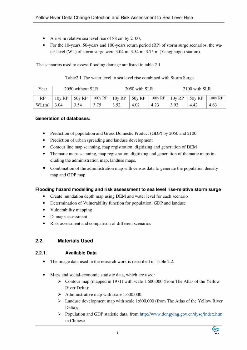
• A rise in relative sea level rise of 88 cm by 2100; • For the 10-years, 50-years and 100-years return period (RP) of storm surge scenarios, the wa-
ter level (WL) of storm surge were 3.04 m, 3.54 m, 3.75 m (Yangjiaogou station). The scenarios used to assess flooding damage are listed in table 2.1
Table2.1 The water level to sea level rise combined with Storm Surge
Year 2050 without SLR 2050 with SLR 2100 with SLR
RP 10y RP 50y RP 100y RP 10y RP 50y RP 100y RP 10y RP 50y RP 100y RP
WL(m) 3.04 3.54 3.75 3.52 4.02 4.23 3.92 4.42 4.63 Generation of databases:
• Prediction of population and Gross Domestic Product (GDP) by 2050 and 2100 • Prediction of urban spreading and landuse development • Contour line map scanning, map registration, digitizing and generation of DEM • Thematic maps scanning, map registration, digitizing and generation of thematic maps in-
cluding the administration map, landuse maps.
• Combination of the administration map with census data to generate the population density map and GDP map.
Flooding hazard modelling and risk assessment to sea level rise-relative storm surge
• Create inundation depth map using DEM and water level for each scenario • Determination of Vulnerability function for population, GDP and landuse • Vulnerability mapping • Damage assessment • Risk assessment and comparison of different scenarios
2.2. Materials Used
2.2.1. Available Data
• The image data used in the research work is described in Table 2.2.
• Maps and social-economic statistic data, which are used: ¾�Contour map (mapped in 1971) with scale 1:600,000 (from The Atlas of the Yellow
River Delta); ¾�Administrative map with scale 1:600,000; ¾�Landuse development map with scale 1:600,000 (from The Atlas of the Yellow River
Delta); ¾�Population and GDP statistic data, from http://www.dongying.gov.cn/dysq/index.htm
in Chinese

Yellow River Delta Change Detection and Risk Assessment to Sea Level Rise
9
¾�Storm surge record (from The Atlas of the Yellow River Delta) ¾�Tidal data (from State Marine Institute)
For change detection of the coastline, Landsat, ERS1/2, and Aster three types of images were applied. Table 2.3 shows the characteristics of those sensors. Table 2.2 Characteristics of the used image data Code Sensor Instrument Acquired Date Local time
ytm9204 Landsat5 TM April 24, 1992 10:00 ytm9305 Landsat5 TM May 5,1993 10:00 ytm9404 Landsat5 TM April 24, 1994 10:00 Ytm96 Landsat5 TM Missing date 10:00 ytm0005 Landsat7 ETM+ May 2,2000 10:12 Ers92 ERS1 SAR Apr 22,1992 10:44 Ers96 ERS2 SAR Jan 5,1996 10:44 Ers98 ERS2 SAR Aug 1,1998 22:19 Ers99 ERS2 SAR Dec 11,1999 10:44 Ast01 Aster VNIR March 18, 2001 11:09
2.2.2. Software
Ilwis3.0, ERDAS and ENVI software are mainly used for the study.

Yellow River Delta Change Detection and Risk Assessment to Sea Level Rise
10
Table 2.3 Sensor characteristics
Characteristic Sensor Band number
SPECTRAL RANGE
Ground Resolu-tion (m)
Temporal resolution
EQUATORIAL CROSSING
INCLINATION:
SUNSYNCHRONOUS,
Swath Width (km)
LandsatTM LandsatETM
Band1 Band2 Band3 Band4 Band5 Band6 Band7 Pan(ETM)
0.45--0.53µm
0.52--0.60µm
0.63--0.69µm
0.76--0.90µm
1.55--1.75µm
10.4--12.5µm
2.08--2.35µm
0.52-0.90µm
30 30 30 30 30 60 30 15
16 days DESCENDING NODE:
10:00AM +/- 15MIN
98.2 DEGREES
185
VNIR Band1 Band2 Band3N Band3B*
0.52--0.60µm
0.63--0.69µm
0.76--0.86µm
0.76--0.86µm
15 15 15 15
SWIR Band4 Band5 Band6 Band7 Band8 Band9
1.60--1.70µm
2.14--2.18µm
2.18--2.22µm
2.23--2.28µm
2.29--2.36µm
2.36--2.43µm
30 30 30 30 30 30
Aster
TIR Band10 Band11 Band12 Band13 Band14
8.12--8.47µm
8.47--8.82µm
8.92--9.27µm 10.25-10.95µm
10.95-11.65µm
90 90 90 90 90
16 days 10:30 ± 15 min. am
98.2deg± 0.15deg
60
ERS1 C-band 5.7cm 30 35days 98.5deg 100 ERS SAR ERS2 C-band 5.7cm 30 35days 98.5deg 100
Yellow River Delta Change Detection and Risk Assessment to Sea Level Rise
11
2.3. flowchart of methodology
2.3.1. Yellow River Delta coastline change detection
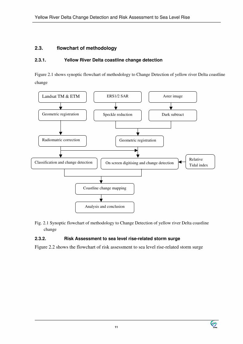
Figure 2.1 shows synoptic flowchart of methodology to Change Detection of yellow river Delta coastline
change
Fig. 2.1 Synoptic flowchart of methodology to Change Detection of yellow river Delta coastline
change
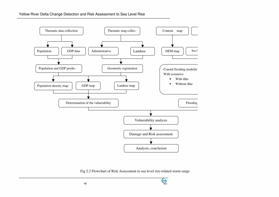
2.3.2. Risk Assessment to sea level rise-related storm surge
Figure 2.2 shows the flowchart of risk assessment to sea level rise-related storm surge
Landsat TM & ETM ERS1/2 SAR Aster image
Geometric registration Dark subtract Speckle reduction
Geometric registration Radiomatric correction
Classification and change detection On screen digitising and change detection Relative Tidal index
Coastline change mapping
Analysis and conclusion
Yellow River Delta Change Detection and Risk Assessment to Sea Level Rise
12
Fig 2.2 Flowchart of Risk Assessment to sea level rise-related storm surge
Population and GDP predic-
Thematic map collec- Contour map
Population Sea level rise data
DEM map GDP data Landuse Administrative
Geometric registration
Population density map GDP map Landuse map
Flooding hazard mapDetermination of the vulnerability
Damage and Risk assessment
Analysis, conclusion
Thematic data collection
Vulnerability analysis
Coastal flooding modelling by 2050 and by 2100 With scenarios:
• With dike • Without dike
•••
Yellow River Delta Change Detection and Risk Assessment to Sea Level Rise
13
3. Description of the Study Area
3.1. Description of the Yellow River Delta
3.1.1. Location and general geographic background
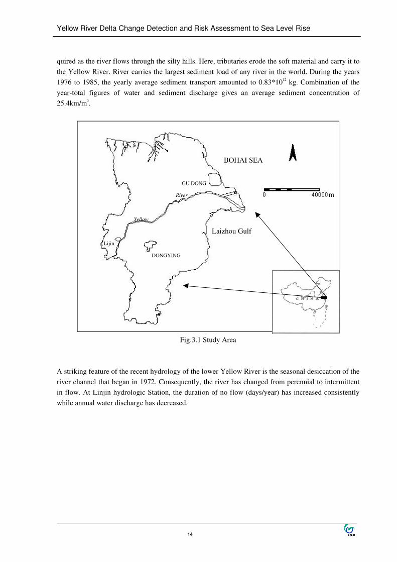
The study area of the Modern Yellow River Delta, is located in the North of Shangdong Province, North China, within latitudes 36016’ ’ 00’ ’ -38013’ ’ 00’ ’ and longitudes 118005’ ’ 00’ ’ -119023’ ’ 00’ ’ . It has an area of 6000km2 in 2000. It is a relatively low lying, flat area. The height on the deltaic apex is 9 m higher than the mean sea water level; the average slope of the land is less than 0.1%. The geo-logic history of the Modern YRD is less than 100 years. The construction of the modern delta mainly occurred after the northward shifting of the Yellow River in 1855. Restrained by the embankment from Lijin country to upstream in Henan and Shandong provinces, the destination of the water and sediments turned from the Yellow Sea to the Bohai Sea. From Lijin to downstream, with the segmen-tal extend of the man-made dykes, and also affected by the Coriolis force, the orientation of the river mouth changed from North and Northeast to East and Southeast. From Lijin to downstream, the lower research of the main stream shifted southward near Laizhou Bay. The river thus produced several sub-deltas in order, just like a Chinese fan. From 1976 to now, there are apparent changes for the Modern YRD, which has become the centre of the second largest oil field in China, with the development of rich oil and gas resources since 1960s. The potential for future economic development is booming. Figure 3.1 shows the study area.
3.1.2. Discharge of the Yellow River
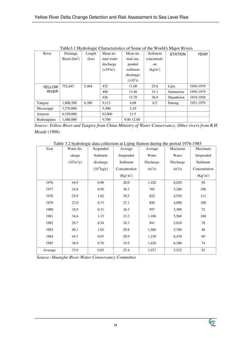
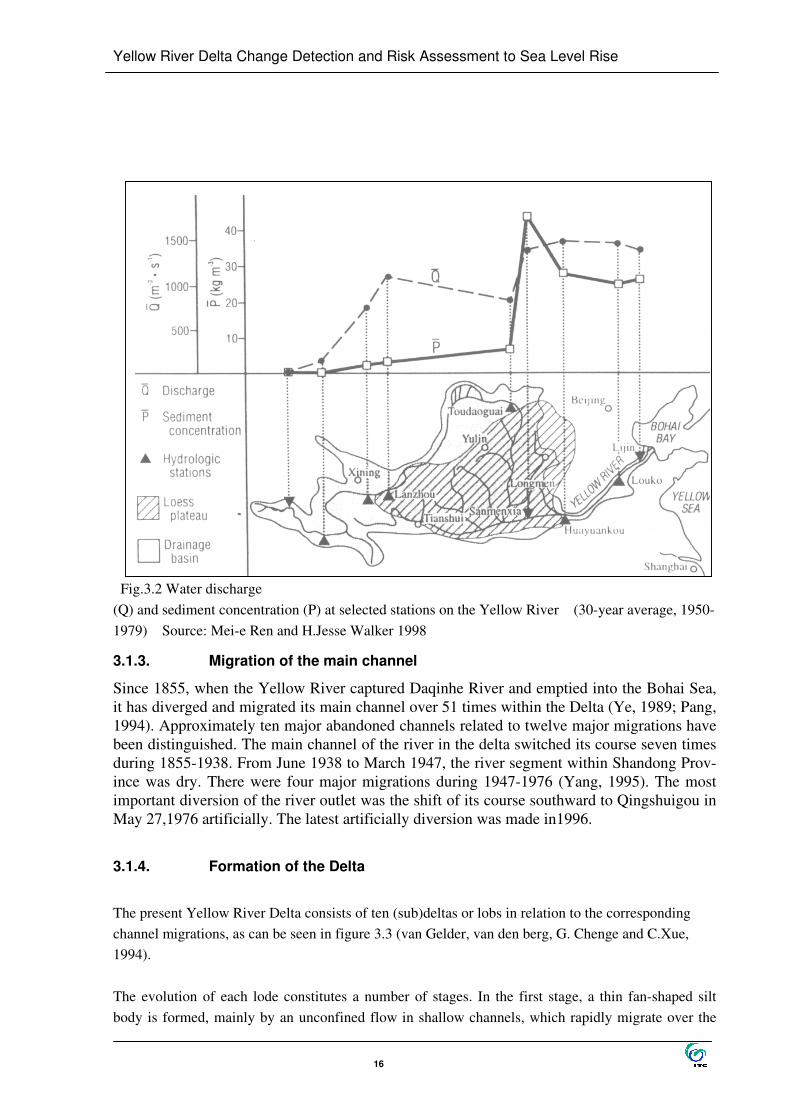
The Yellow River, is known as the Huanghe (Huang means "yellow", He means "river") because of its high sediment content in “ yellow” colour. It has a length of 5,464km and a drainage basin of 752,443km2. It is China's second longest river, after the Yangtze River. It starts in Tibet and flows eastwards in a great arc, crossing through the Great Wall of China twice and then passing through silt (loess) hills before flowing out onto the vast North China Plain into the Bohai Sea. Much of this re-gion experiences only low rainfall totals and so discharge is low compared to the Yangtze River. The rainfall totals vary greatly from year to year and so the discharge is very variable. Measured at the Linjing Hydrologic Station, about 100km upstream from the present river mouth, the river mean annual flow is 432*108 m3 (about 8% of that the Mississippi River) and its suspended sediment load is about 11*108 tons (about five times that of Mississippi River) Table 3.1, Table 3.2 (Yang, 1995); Figure3.2 show Yellow River discharge and sediment concentration at selected stations (30-year average, 1950-1979). (Mei-e Ren and H.jesse Walker 1998). In the upper part of the catch-ment the river water is completely clear. The silt, and therefore the yellow color of the water are ac-
Yellow River Delta Change Detection and Risk Assessment to Sea Level Rise
14
quired as the river flows through the silty hills. Here, tributaries erode the soft material and carry it to the Yellow River. River carries the largest sediment load of any river in the world. During the years 1976 to 1985, the yearly average sediment transport amounted to 0.83*1012 kg. Combination of the year-total figures of water and sediment discharge gives an average sediment concentration of 25.4km/m3.
Fig.3.1 Study Area
A striking feature of the recent hydrology of the lower Yellow River is the seasonal desiccation of the river channel that began in 1972. Consequently, the river has changed from perennial to intermittent in flow. At Linjin hydrologic Station, the duration of no flow (days/year) has increased consistently while annual water discharge has decreased.
GU DONG
Yellow
DONGYING
Lijin
River
BOHAI SEA
Laizhou Gulf
m
Yellow River Delta Change Detection and Risk Assessment to Sea Level Rise
15
Table3.1 Hydrologic Characteristics of Some of the World’s Major Rivers River Drainage
Basin (km2) Length (km)
Mean an-nual water discharge (×108m3)
Mean an-nual sus-pended
sediment discharge (×108 t)
Sediment concentrati-
on (kg/m3)
STATION YEAR
432 11.00 25.6 Lijin 1950-1979
408 13.40 33.1 Sanmenxia 1958-1979 YELLOW
RIVER 752,443 5,464
426 15.70 36.9 Shaanhsien 1919-1958
Yangtze 1,808,500 6,300 9,113 4.68 0.5 Datong 1951-1979
Mississippi 3,270,000 5,300 2.10
Amazon 6,150,000 63,000 11.5
Brahmaputra 1,480,000 9,700 9.00-12.00
Source: Yellow River and Yangtze from China Ministry of Water Conservancy. Other rivers from R.H. Meade (1996)
Table 3.2 hydrologic data collection at Lijing Station during the period 1976-1985
Year Water dis-
charge
(109m3/y)
Suspended
Sediment
discharge
(1012kg/y)
Average
Suspended
Sediment
Concentration
(Kg/ m3)
Average
Water
Discharge
(m3/s)
Maximum
Water
Discharge
(m3/s)
Maximum
Suspended
Sediment
Concentration
(Kg/ m3)
1976
1977
1978
1979
1980
1981
1982
1983
1984
1985
44.9
24.8
25.9
27.0
18.9
34.6
29.7
49.1
44.7
38.9
0.90
0.95
1.02
0.73
0.31
1.15
0.54
1.02
0.93
0.76
20.0
38.3
39.5
27.1
16.3
33.2
18.3
20.8
20.9
19.5
1,420
785
822
856
597
1,100
941
1,560
1,230
1,420
8,020
5,280
4,550
4,090
3,300
5,560
5,810
5,760
6,470
6,380
58
196
111
109
72
100
78
48
69
74
Average 33.9 0.83 25.4 1,073 5,522 92
Source: Huanghe River Water Conservancy Committee
Yellow River Delta Change Detection and Risk Assessment to Sea Level Rise
16
Fig.3.2 Water discharge (Q) and sediment concentration (P) at selected stations on the Yellow River (30-year average, 1950-1979) Source: Mei-e Ren and H.Jesse Walker 1998
3.1.3. Migration of the main channel
Since 1855, when the Yellow River captured Daqinhe River and emptied into the Bohai Sea, it has diverged and migrated its main channel over 51 times within the Delta (Ye, 1989; Pang, 1994). Approximately ten major abandoned channels related to twelve major migrations have been distinguished. The main channel of the river in the delta switched its course seven times during 1855-1938. From June 1938 to March 1947, the river segment within Shandong Prov-ince was dry. There were four major migrations during 1947-1976 (Yang, 1995). The most important diversion of the river outlet was the shift of its course southward to Qingshuigou in May 27,1976 artificially. The latest artificially diversion was made in1996.
3.1.4. Formation of the Delta
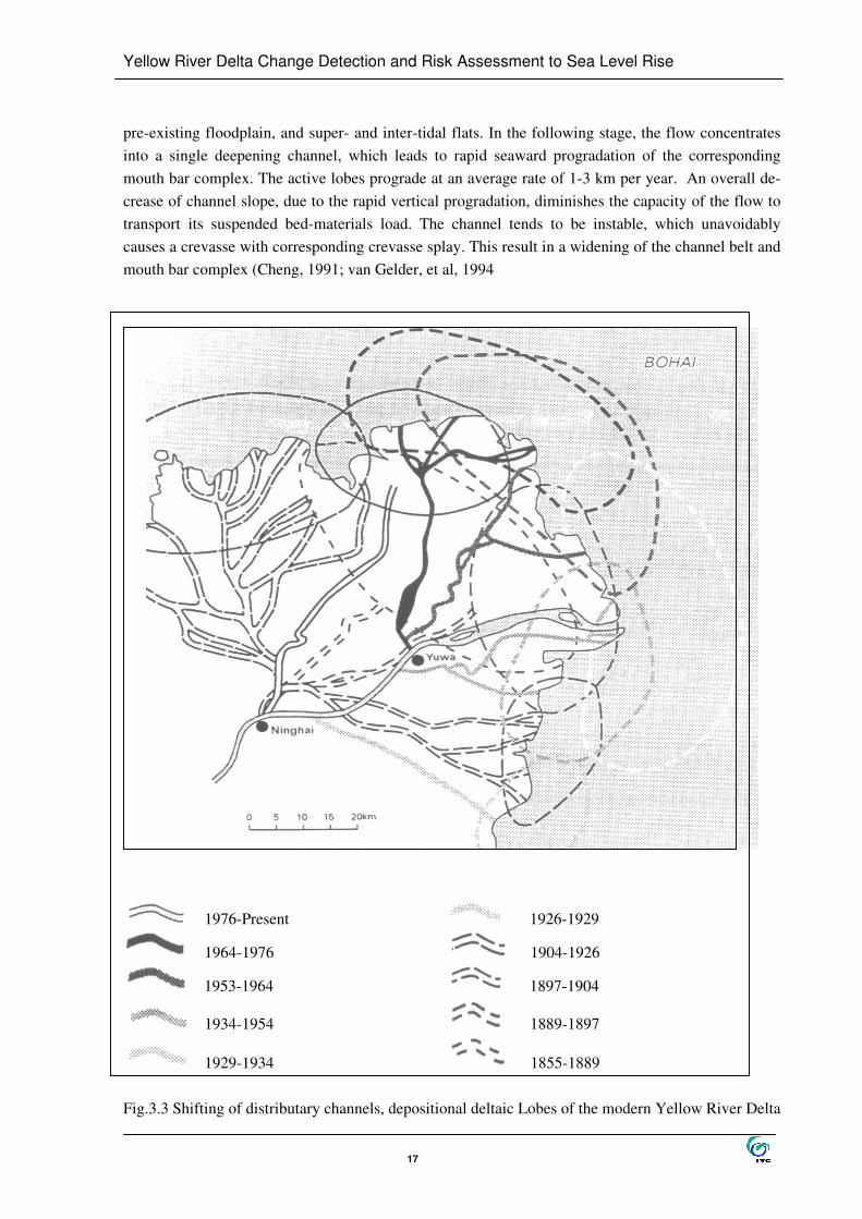
The present Yellow River Delta consists of ten (sub)deltas or lobs in relation to the corresponding channel migrations, as can be seen in figure 3.3 (van Gelder, van den berg, G. Chenge and C.Xue, 1994). The evolution of each lode constitutes a number of stages. In the first stage, a thin fan-shaped silt body is formed, mainly by an unconfined flow in shallow channels, which rapidly migrate over the
Yellow River Delta Change Detection and Risk Assessment to Sea Level Rise
17
pre-existing floodplain, and super- and inter-tidal flats. In the following stage, the flow concentrates into a single deepening channel, which leads to rapid seaward progradation of the corresponding mouth bar complex. The active lobes prograde at an average rate of 1-3 km per year. An overall de-crease of channel slope, due to the rapid vertical progradation, diminishes the capacity of the flow to transport its suspended bed-materials load. The channel tends to be instable, which unavoidably causes a crevasse with corresponding crevasse splay. This result in a widening of the channel belt and mouth bar complex (Cheng, 1991; van Gelder, et al, 1994
1976-Present 1926-1929
1964-1976 1904-1926
1953-1964 1897-1904
1934-1954 1889-1897
1929-1934 1855-1889 Fig.3.3 Shifting of distributary channels, depositional deltaic Lobes of the modern Yellow River Delta

Yellow River Delta Change Detection and Risk Assessment to Sea Level Rise
18
Source: Van Gelder, et al, 1994
3.1.5. Coastline change
A general sequence of coastline evolution during 1855-1985 has been set up through the comparison of maps prepared at different stages, combined with historical literature, field investigation, and im-age interpretation. Figure 3.4 presents a coastline change map during 1855-1989. Given the course-running period of 134 years, the progradational rate of the coastline is, therefore, 160 meters per year. During 1855-1959, the Coastline advanced on the average 14 km seaward. In a period of 94-years, the progradational rate is 152 meters per year. Since 1959, the coastline has prograted at a relatively higher rate of 224 meters per year. This is due to the fact that the apex of delta has moved down-stream and the scope of channel migration has limited.
Fig.3.4 Coastline change in the modern Yellow River Delta 1855-1989 Source: Mei-e Ren and H.jesse Walker 1998
Yellow River Delta Change Detection and Risk Assessment to Sea Level Rise
19
3.2. Hydraulic Setting of The Bohai Sea
3.2.1. General Topographic Features
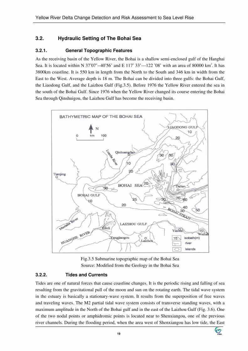
As the receiving basin of the Yellow River, the Bohai is a shallow semi-enclosed gulf of the Hanghai Sea. It is located within N 37o07’ --40o56’ and E 117o 33’ ---122 o08’ with an area of 80000 km2. It has 3800km coastline. It is 550 km in length from the North to the South and 346 km in width from the East to the West. Average depth is 18 m. The Bohai can be divided into three gulfs: the Bohai Gulf, the Liaodong Gulf, and the Laizhou Gulf (Fig.3.5). Before 1976 the Yellow River entered the sea in the south of the Bohai Gulf. Since 1976 when the Yellow River changed its course entering the Bohai Sea through Qinshuigou, the Laizhou Gulf has become the receiving basin.
Fig.3.5 Submarine topographic map of the Bohai Sea Source: Modified from the Geology in the Bohai Sea
3.2.2. Tides and Currents
Tides are one of natural forces that cause coastline changes. It is the periodic rising and falling of sea resulting from the gravitational pull of the moon and sun on the rotating earth. The tidal wave system in the estuary is basically a stationary-wave system. It results from the superposition of free waves and traveling waves. The M2 partial tidal wave system consists of transverse standing waves, with a maximum amplitude in the North of the Bohai gulf and in the east of the Laizhou Gulf (Fig. 3.6). One of the two nodal points or amphidromic points is located near to Shenxiangou, one of the previous river channels. During the flooding period, when the area west of Shenxiangou has low tide, the East

Yellow River Delta Change Detection and Risk Assessment to Sea Level Rise
20
has high tide; and vice versa. The situation is the same during the ebbing stage. Most of the estuary is characterized by an irregular semi-diurnal (1/2 day) southward flood tide and northward ebb tide. The tidal range averages 0.6-0.8 m near the Shenxiangou and increases southward and westward to 1.5-2.0 m. The maximum range can be 5.06 m. The maximum velocity of the tidal currents in the area with 5-15 m in the depth outside Shenxiangou can be 1.5 m/s, showing a relatively strong scouring ability. Silts are transported easily in this area without much deposition. The velocity tends to decrease to-wards both sides. They are 0.4-0.6 m/s at the north of the Bohai Gulf, and 0.8m/s at the present river mouth, respectively.
Fig.3.6 M2 partial tidal wave system in the Bohai Sea
Source: Wang 1984 The tidal head is limited to 30 km inland from the river mouth. As sandbars develop towards the sea and the riverbed is silting up, the tidal influence tends to move towards the sea. When N-NE-oriented gusty winds occur for a long time, an exceptional rise of the water level will exist near the sea, and the distance of effected stream may be over 50 km. When the Yellow River is at high-water season, there are usually no upward (tidal) currents. While at relatively low-water season, tidal currents can intrude upstream the river mouth (Yang, 1995).
3.2.3. Wind and Storm Surge
Owing to a monsoon with high seasonal variability, the wind-orientation changes during different sea-son. In the winter, the north-oriented winds dominate; in the summer, the south-oriented winds domi-nate. Generally, the maximum velocity of the wind occurs around April and May. The gusty winds with maximum velocity sometimes travel at 40m/s. storm winds usually occur in July and August.

Yellow River Delta Change Detection and Risk Assessment to Sea Level Rise
21
gust. The most frequent winds are SW-oriented winds with a frequency of 10.9%. This is followed by the NNE-oriented winds with a frequency of 1.42%. Strong winds with a velocity over 17.2m/s occur on the average 35 days per year, while strong winds with velocity of over 12.8m/s occur on average 57 days per year (Ren, et al., 1980). Winds with N and NNE orientations have posed the strongest effect on the Yellow River Delta. The storm surge in the Yellow River Delta mainly results from NE-oriented winds. After a long time strong wind action, an exceptional rise of the sea water level along the coast can occur. As a result of the flat topography at the mouth area, even 3 m high storm surge can intrude inland tens kilometers. According to uncompleted statistics, from 1840-1940, disastrous storm surges occurred four times (1846, 1890, 1902, and 1938). In 1890, the storm surge caused a 4m rise of sea level, flooding an area of 4,500 km2. While in 1938, the storm surge caused a 3.6-4.1 m rise of the sea level, flooding an area of 3,000 km2. Since 1949, disastrous storm surges have occurred at least six times. In April 5-7, 1964, a very strong storm surge occurred with a maximum 6.2 m rise of sea level, causing flooding until 50 km inland and resulting in the death of over 600 people. In order to defend the invasion of storm surge a tide-resistance dike of 138 km in length was con-structed by Shengli Oilfield. Its standard of height is in accordance with the storm surge that happens once in 20 years or 50 years. But the south dike along the Yellow River Delta is particularly weak.
3.2.4. Wind Wave
Wind waves are the most active factor for the transport of sediment along the shallow coast. In the coastal area of Bohai Gulf, the water is shallow and always frozen in winter, and the wave amplitude is relatively low. Within this area, the average amplitude of the waves is 0.4m with a period of about 1.9s during March and November. According to Hou, the possible amplitude for waves occurring once in 100 years may be 7 m with a period of 10 second. Wind can stir mud in shallow beaches, and make it easy to transported by currents. On the other hand, it can produce rip currents that transport silts
3.2.5. Residual Currents
The residual currents are most important force that transport silts deposited at the river mouth. Aver-age residual currents in the surface are 20-30cm/s. In the near bottom layers, the residual current has the characteristics of a compensation current that moves mainly westward at a speed of 5-15cm/s. The residual current in the surface layers moves southward in winter and northward or northeast in sum-mer.
3.3. Sea Level Rise and Land Subsidence
3.3.1. Sea Level Rise
Warmer temperatures are expected to cause a rise of sea level. The Intergovernmental Panel on Cli-mate Change (IPCC) estimates that sea level will rise 9 to 88 cm by the year 2100 (Fig.3.7). A recent study estimated that the global sea level has a 50 percent chance of rising 45 cm by the year 2100, but a 1-in-100 chance of a rise of about 110 cm. Located at the meeting point of the Yellow River and The Bohai Sea, The Yellow River Delta is more sensitive due to its low lying and rapid land subsidence. The estimated relative sea level rise rate in the Yellow River Delta is 8 mm/year and the sea level rise will be 48 cm by the year 2050. This will lead to critical impacts such as the frequency of storm surge and El-Niño events to strengthen hydrodynamics, beach erosion, and landward retreat, wetland loss, saltwater intrusion, and

Yellow River Delta Change Detection and Risk Assessment to Sea Level Rise
22
land salinization, etc. Sea level rise also will increase risk of flooding and storm damage. (http://www.ea.gov.au/ssd/publications/ssr/149.html)
Fig. 3.7 The estimated Global Sea Level Rise
Source: IPCC Third Assessment Report (2001) (http://www.epa.gov/globalwarming/climate/future/sealevel.html)
3.3.2. Land Subsidence
Land subsidence is the other major factor to cause a relative sea level rise. Table 3.3 shows relative sea level rise changes from1950’ s to 1980’ s at stations in the YRD. Two most remarkable facts can be pointed out. First the Bohai coast is an area of severe recent seismic activity. The great Tangshan and Haicheng earthquakes with a magnitude of 7.8 and 7.3 (Richter Scale) and a submarine earthquake in the Baohai Sea of magnitude 7.4 took place in 1976, 1975 and 1969. The Tangshan earthquake caused a dramatic relative sea level rise which can be seen in the tidal gauge record of Tanggu Station. Total subsidence at Tanggu was 2.85m during 1955 and 1985, averaging was 9.3cm/year, in 1976, the ground subsided 23.0cm. Tectonically, the Tanggu area is crossed by the large Haihe fault, along which small earthquakes are frequent. Recently oil exploitation and large amounts of over-extraction has become the major factor for land subsidence.
Table 3.3 Relative sea level changes at station in the Yellow River delta Station Rate of sea level change (cm/year) Period
Yingkou +0.11 1952-1971 Huludao +0.19 1955-1981
Qinghuangdao +0.21 1956-1980 Tanggu +0.81 1950-1981
Yangjiaoguo +0.19 1952-1978 Longkou +0.25 1961-1981

Yellow River Delta Change Detection and Risk Assessment to Sea Level Rise
23
4. COASTLINE CHANGE DETECTION
This chapter describes computer-assisted operations for change detection of the most active YRD coastline. The image processing includes image correction and registration, and spectral enhancement of Landsat, ERS1/2, and Aster images. Image classification, image differencing, post-classification image overlaying and image interpretation were applied to present coastline change detection. Finally through near 10 years change result of YRD, an analysis of coastline change was carried out.
4.1. Image Processing
4.1.1. Landsat and Aster image processing
• Radiometric Correction
The method of correction used in this study is based on radiometric rectification methods developed by F.G. Hall, D.E.Strebel, J.E.Nickeson and S.J.Goetz (1991). The technique has the advantage of not requiring sensor calibration or atmospheric turbidity data. The method correct images from a common scene in a relative, rather than an absolute sense. The image is rectified relative to a selected reference image. The underlying assumption in this approach is that an image always contains at least some pixels that have the same average surface reflectance between images resulting from the only change in the spectral signature of these pixels between images resulting from differences in atmospheric, solar irradiance and radiometric conditions. By using a series of “ dark” and “ bright” radiometric con-trol sets, a simple linear rectification algorithm has been constructed. This allows the images to be referenced against each other. The result of the transformation is that the images appear as if they were acquired under the same atmospheric and illumination condition, by a sensor with the same ra-diometric sensitivity. This approach performed well, removing the effects of relative atmospheric dif-ferences to within 1% absolute reflectance for visible and near infrared bands (Yang, 1995).
This method was applied with Ilwis in this study. Figure 4.1 shows the procedures of this radiometric correction method. The result of the transformation is presented in table 4.1 Aster image radiometric correction was carried out with Envi 3.4 software.
• Image to image registration – GCP collection
Image to image registration of Landsat and Aster image was carried out in ILWIS. ERS1/2 image reg-istration was performed in ERDAS. More attention should be paid on collecting at least 12 well dis-tributed GCPs for each image rectification. The GDP collection was time-consuming, particularly for ERS images and Aster images. The study area only occupies one-tenth on the total image. Around the

Yellow River Delta Change Detection and Risk Assessment to Sea Level Rise
24
most active delta is Bohai Sea. It was difficult to find the well distributed GCPs. This activity con-sumed too much time. The Landsat images ytm94 (Apr.24,1994), ytm92 (Apr.4,1992), ytm93 (May. 5,1993) have been geo-referenced, Ytm94 was selected as master map to georeference landsat7 ETM images ytm00 (May.2,2000). For b1,b2,b3,b4,b5,b7, 21 GCPs were collected and the sigma value was 0.4692. For panchromatic band8, 24 GCPs were applied and a sigma value of 0.4215 was obtained. For Aster 2001 image, b1,b2,b3 were georeferenced through 15 GCPs with a sigma value of 0.4126. b4-b9 were rectified using 12 GCPs with a sigma value of 0.4673. The Resampling method Nearest Neighbour was selected to resample those images.
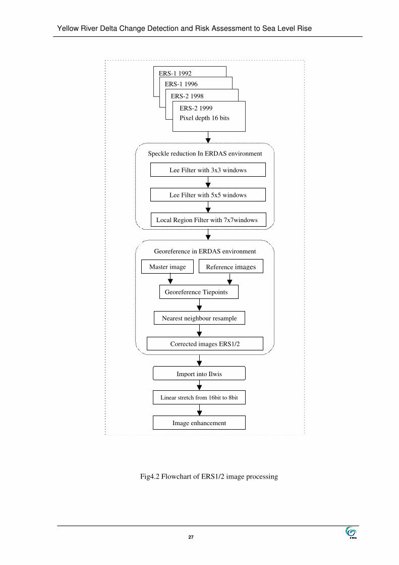
4.1.2. ERS1/2 image processing
Radar SAR image is active sensor image, its processing is different from optical image. The figure 4.2 shows the flowchart of ERS images
• Speckle reduction and adjusting of brightness For the research work 4 scenes of SAR Precision Image (ERS1/2.SAR.PRI) with a 30 m spatial reso-
lution are used. The Precision Image is a multi-look (speckle-reduced), ground range, system cor-
rected image. The product is calibrated and corrected for the SAR antenna pattern and range-
spreading loss; radar backscatter can be derived from the product for geophysical modelling, but no
correction is applied for terrain-induced radiometric effects. The image is not geo-coded, and terrain
distortion (foreshortening and layover) has not been removed. Although the Radar images speckle has
been reduced, it still exist on the images. For better interpretation it is necessary to reduce the speckle
further. Therefore a Lee filter and local region filter were used in ERDAS. The result is satisfactory.
Many speckles were reduced, which makes the identification between land and water easier. The
Figure 4.3 shows the ERS2 image (Dec.22, 1999) after and before speckle-reduction.
Because the luminance of the original Radar images is various, different processing procedures were applied for image enhancement. After reducing speckle, the ERS92, ERS96, ERS99 Radar images were adjusted for brightness. This operation was performed In ERDAS environment using Adjust Brightness function. But for the ERS98 image, when we compare before adjusted brightness image with those after adjusted brightness one, the luminance contrast of the un-adjusted brightness image is better than the adjusted one.
• Image to image registration – GCP collection
ERS1/2 image registration was performed in ERDAS. As mentioned in 4.1.1, it also consumed too much time. Theoretically, the SAR image should be ortho-rectified using DEM or constant elevation value. The elevation of the delta is between 0 and 9 m above mean sea water level with a steepness of less than 0.1%. The study area is flat enough to neglect the effects of topographic relief displacement.

Yellow River Delta Change Detection and Risk Assessment to Sea Level Rise
25
Slave images (SI) reference image (RI)
Fig.4.1 the procedures of radiometric correction.
Table 4.1 Statistics about the result of radiometric correction Reference image ( ytm94 ) Apr.24, 1994
Slave image TM (ytm92) Apr.4, 1993
Slave image TM (ytm93) May 5,1993
Slave image ETM (ytm00) May 2,2000
Landsat Image
Mean Std.Dev Mean Std.Dev Mean Std.Dev Mean Std.Dev Before correction: Band 1 Band 2 Band 3 Band 4 Band 5 Band 7
94 45 51 47 58 32
31.77 16.23 21.83 25.03 40.49 23.92
95 43 48 38 53 30
31.40 14.77 18.69 19.50 40.24 24.21
122 54 65 45 66 112
36.42 16.71 24.40 24.16 50.07 34.89
113 95 96 46 71 60
10.13 14.60 31.51 26.25 56.27 48.42
After correction: Band 1 Band 2 Band 3 Band 4 Band 5 Band 7
94 45 51 47 58 32
31.77 16.23 21.83 25.03 40.49 23.92
88 41 44 41 55 31
30.00 15.98 21.48 25.81 40.24 22.00
92 44 48 44 52 37
26.51 12.44 15.43 20.44 32.93 34.22
96 42 41 30 45 25
7.85 6.33 13.24 27.32 39.45 22.30
Therefore in this study the four ERS1/2 images were rectified without DEM. Table 4.2 shows the numbers of GCPs and sigma values.
Landsat TM and ETM images (band 1—7) Landsat TM and ETM images (band 1—7)
Selection of radiometric control sets Selection of radiometric control sets
Read mean value for the bright and dark set Bs1—Bs7 and Ds1---Ds7
Read mean value for the bright and dark set Br1—Br7 and Dr1---Dr7
Calculation of the transformation coefficients: mi:=(Bri-Dri)/(Bsi-Dsi) bi:=(Bsi*Dri-Dsi*Bri)/(Bsi-Dsi) i=1,2,3,4,5,7
Transformation operation: Mapcalc: CSI:=mi*SI+bi

Yellow River Delta Change Detection and Risk Assessment to Sea Level Rise
26
Table 4.2 ERS image geometric correction and registration Image ERS1 92 ERS2 96 ERS2 98 ERS2 99 RMS 0.8550 0.7235 0.5909 0.7851 GCPs 14 15 18 19
• Image translation
The SAR images were delivered in a 16-bit format, having 65,536 possible pixel values. The conver-sion to the 8-bit format is considered a standard procedure for satellite SAR images (Van der Sanden, 1997). Some information is always lost during the operation, but the conversion allows an increase in image processing speed and resulting images require much less storage capacity. For the GIS proce-dure, after image geometric correction (see section 4.1.3), SAR image should be converted into Ilwis from ERDAS. In ILWIS only 8-bit format is supported. The four SAR images were rescaled from 16-bit to 8-bit in ILWIS. As a result the new images had pixel values varying from 0 to 255.
(a) Fig.4.3 The SAR image after (a) and before (b) speckle-reduction (ERS2 image, Dec.22, 1999)
(b)
Yellow River Delta Change Detection and Risk Assessment to Sea Level Rise
27
Fig4.2 Flowchart of ERS1/2 image processing
ERS-1 1992
ERS-1 1996
ERS-2 1998
ERS-2 1999 Pixel depth 16 bits
Speckle reduction In ERDAS environment
Lee Filter with 3x3 windows
Lee Filter with 5x5 windows
Local Region Filter with 7x7windows
Linear stretch from 16bit to 8bit
Image enhancement
Georeference in ERDAS environment
Master image Reference images
Corrected images ERS1/2
Import into Ilwis
Georeference Tiepoints
Nearest neighbour resample

Yellow River Delta Change Detection and Risk Assessment to Sea Level Rise
28
4.2. Image classification and change detection
4.2.1. Image classification
For the detection of coastline change on the image, the threshold to differentiate between wa-ter and land have to be determined. In this section the techniques for water-land line classification was performed. For Landsat images, with the increase of bands, the spectral reflectance value of the water body decreases, i.e. b1>b2>b3>b4>b5>b7. Meanwhile, band 5,7 can be used to determine threshold to mask the water out. Two infrared band Landsat images ytm94b5 (Apr.24, 1994) and ytm00b5 (May.2, 2000) were se-lected to separate land and water body. The first the linear stretching was performed to ytm00b5 and ytm94b5 image. Through histograms analysis (Figure 4.4 and Figure 4.5) and image interpretation the threshold between water and land was determined. This is 65 and 48 DN value for ytm94b5 and ytm00b5 image classification. The image classification was performed with the ILWIS map calculation operation. The calculation formula is: Y94WL:=iff(ytm94b5>65,1,0) Y00WL:=iff(ytm00b5>48,1,0) Where 1 present land; 0 present water A majority filter to smooth the classified images carried out. The figure 4.6 and 4.7 present the output map.
4.2.2. Change detection
Multi-temporal change detection involves discrimination of difference in the state of an object be-tween images of different dates. Digital change detection provides automatic correlation and compari-son of two sets of imageries covering the same geographical area at different times and displaying the changes and their locations. The fundamental promise is that the changes in land cover must result in changes in radiance values (DN values), which should be large with respect to radiance change caused by other factors (Ingram, et al, 1981). A variety of techniques for change detection based on comparison of multi-temporal digital remote sensed data have been developed (Singh, 1989). Some brief remarks on the advantages and disadvan-tages of those techniques have been given by Yang (1995), which can be seen in Table 4.3. Among those techniques, image differencing and image overlaying were applied to detect the change of YRD.

Yellow River Delta Change Detection and Risk Assessment to Sea Level Rise
29
Special mention: when image differencing and post-classification Image overlaying operations were carried out, as the tidal data was not available, the tidal effect was not taken into consideration at that moment. In section 4.3.1 you will find the result is the difference from those along the profile B.
Fig.4.4 The histogram of image ytm94b5 Fig. 4.5 The histogram of image ytm00b5
Fig 4.6 The classification map of ytm94b5 Fig. 4.7 The classification map of ytm00b5
• Image differencing operation Image differencing operation is a procedure of image arithmetic change detection. For different tem-poral images, the arithmetic operation: image change=image(2)-image(1)+C was calculated. Where image (2) and image (1) are two different date images, C is a compensation factors to ensure positive result. Figure 4.8 presents a change detection image through image differencing technique. The first image ytm94b5 and ytm00b5 have been classified according to the procedure in section 4.2.1. They are two
Water Land
Water Land

Yellow River Delta Change Detection and Risk Assessment to Sea Level Rise
30
binary maps showing the land and water classification in 1994 and 2000. The output map includes three units (table 4.4)

Yellow River Delta Change Detection and Risk Assessment to Sea Level Rise
31
Table 4.3 Overview of change detection technique Analytical techniques used to de-tect changes
Image differencing (ID) Image rationing (IR) Principal components analysis (PCA)
Change vector analysis (CVA)
Image fusion technique (IF)
Image overla
Basic opera-tions
Output=input (t2)-input(t1)+C, where C is a compensation constant
Output=input (t2) /input(t1)*C, where C is a compensation constant
Image taken from dif-ferent data are trans-formed into a new or-thogonal reference sys-tem based on the co-variance matrix of the sample set
Analysing the direction and magnitude of change from the first to the sec-ond data
It assigns red, green, and blue colours to three images taken on different dates, using standard false colour compos-ite technique.
By using prothe two input images of different dates can be combined to produce an cross image with a cross image with a cross table, which can be used in the change detection analsis
Remarks It is the most widely used technique for change detection. It is critical in setting the threshold value. It is highly sensitive to misregistration and the existence of mixed pix-els. There is a potential loss of information, e.g. two sets of values may have an identical differenced value
It is a relatively rapid means of identifying areas of change It is critical to select appropriate threshold values It may produce error due to the abnormal distribution on which it based
The data can be recon-structed without noise and redundant informa-tion Even though there are some cases showing positive role of PCA in change detection, the quantitative analysis of the result is short.
It is valuable technique for forest change detection. The performance is sensitive to its parameter set-ting. The reference data set is essen-tially difficult to be available in most cases. The computation load is a formi-dable task
It is easy to perform. The display is direct and easy to understand in case of sample spectral vari-ability, e.g. binary images. For image with high spectral variability, it is essentially impossible to interpret the colour coding
It is the most extensively used technique with high efficiency. It is highly sensitive to misregistration.

Yellow River Delta Change Detection and Risk Assessment to Sea Level Rise
32
Table 4.4 an output of change detection image through image-differencing operation Code Name Explanation
0 Changed Land to water
1 Unchanged Water (1994)-water(2000); land(1994)-land(1994)
2 Changed Water to land
Fig 4.8 Change detection through image differencing Description of map: Value 0: land in 1994 water in 2000 Value 1: without change from 1994 to 2000 Value 2: water in 1994 Land in 2000 From this classification map it is very clear that a new delta appeared and the Yellow River changed its flow direction from Southeast to Northeast. And also along the north coastline erosion is very strong.
• Image overlaying In this operation, the first two registered images were independently classified, after this in Iwils Cross program was applied to overlay between map pairs for post-classification comparison. A cross table was created. By combining the cross table and cross map, the change detection can be defined both qualitatively and quantitatively. In this case two classified image ytm94b5c and image ytm00b5c were selected. The Table 4.5 and Figure 4.9 show the cross table and cross map.
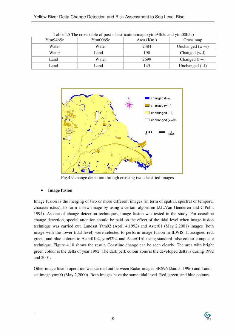
Yellow River Delta Change Detection and Risk Assessment to Sea Level Rise
33
Table 4.5 The cross table of post-classification maps (ytm94b5c and ytm00b5c)
Ytm94b5c Ytm00b5c Area (Km2) Cross map Water Water 2384 Unchanged (w-w) Water Land 190 Changed (w-l)
Land Water 2699 Changed (l-w) Land Land 145 Unchanged (l-l)
Fig.4.9 change detection through crossing two classified images
• Image fusion
Image fusion is the merging of two or more different images (in term of spatial, spectral or temporal characteristics), to form a new image by using a certain algorithm (J.L.Van Genderen and C.Pohl, 1994). As one of change detection techniques, image fusion was tested in the study. For coastline change detection, special attention should be paid on the effect of the tidal level when image fusion technique was carried out. Landsat Ytm92 (April 4,1992) and Aster01 (May 2,2001) images (both image with the lower tidal level) were selected to perform image fusion in ILWIS. It assigned red, green, and blue colours to Aster01b2, ytm92b4 and Aster01b1 using standard false colour composite technique. Figure 4.10 shows the result. Coastline change can be seen clearly. The area with bright green colour is the delta of year 1992. The dark perk colour zone is the developed delta is during 1992 and 2001.
Other image fusion operation was carried out between Radar images ERS96 (Jan. 5, 1996) and Land-sat image ytm00 (May 2,2000). Both images have the same tidal level. Red, green, and blue colours

Yellow River Delta Change Detection and Risk Assessment to Sea Level Rise
34
Fig. 4.10 Image fusion Aster01 b2, ERS92, Aster01 b1 (RGB)
Fig.4.11 Image fusion ytm00b4,b5,ers96 (RGB)
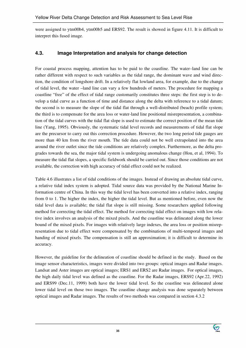
Yellow River Delta Change Detection and Risk Assessment to Sea Level Rise
35
were assigned to ytm00b4, ytm00b5 and ERS92. The result is showed in figure 4.11. It is difficult to interpret this fused image.
4.3. Image Interpretation and analysis for change detection
For coastal process mapping, attention has to be paid to the coastline. The water–land line can be rather different with respect to such variables as the tidal range, the dominant wave and wind direc-tion, the condition of longshore drift. In a relatively flat lowland area, for example, due to the change of tidal level, the water –land line can vary a few hundreds of meters. The procedure for mapping a coastline “ free” of the effect of tidal range customarily constitutes three steps: the first step is to de-velop a tidal curve as a function of time and distance along the delta with reference to a tidal datum; the second is to measure the slope of the tidal flat through a well-distributed (beach) profile system; the third is to compensate for the area loss or water-land line positional misrepresentation, a combina-tion of the tidal curves with the tidal flat slope is used to estimate the correct position of the mean tide line (Yang, 1995). Obviously, the systematic tidal level records and measurements of tidal flat slope are the precursor to carry out this correction procedure. However, the two long period tide gauges are more than 40 km from the river mouth. The tide data could not be well extrapolated into the area around the river outlet since the tide conditions are relatively complex. Furthermore, as the delta pro-grades towards the sea, the major tidal system is undergoing anomalous change (Hou, et al, 1994). To measure the tidal flat slopes, a specific fieldwork should be carried out. Since those conditions are not available, the correction with high accuracy of tidal effect could not be realized. Table 4.6 illustrates a list of tidal conditions of the images. Instead of drawing an absolute tidal curve, a relative tidal index system is adopted. Tidal source data was provided by the National Marine In-formation centre of China. In this way the tidal level has been converted into a relative index, ranging from 0 to 1. The higher the index, the higher the tidal level. But as mentioned before, even now the tidal level data is available; the tidal flat slope is still missing. Some researchers applied following method for correcting the tidal effect. The method for correcting tidal effect on images with low rela-tive index involves an analysis of the mixed pixels. And the coastline was delineated along the lower bound of the mixed pixels. For images with relatively large indexes, the area loss or position misrep-resentation due to tidal effect were compensated by the combinations of multi-temporal images and handing of mixed pixels. The compensation is still an approximation; it is difficult to determine its accuracy. However, the guideline for the delineation of coastline should be defined in the study. Based on the image sensor characteristics, images were divided into two groups: optical images and Radar images. Landsat and Aster images are optical images; ERS1 and ERS2 are Radar images. For optical images, the high daily tidal level was defined as the coastline. For the Radar images, ERS92 (Apr.22, 1992) and ERS99 (Dec.11, 1999) both have the lower tidal level. So the coastline was delineated alone lower tidal level on those two images. The coastline change analysis was done separately between optical images and Radar images. The results of two methods was compared in section 4.3.2

Yellow River Delta Change Detection and Risk Assessment to Sea Level Rise
36
4.3.1. Optical images interpretation and coastline change analysis
Based on the tidal level, the tidal flats can be divided into a number of subunits, such as high, me-dium, and low tidal flats. They are also different in respect to soil, and the variation in water content in relation to the exposure interval. As can be seen in figure 4.12, on Landsat image FCC ytm92 (April, 4,1992), unit 1 exhibits lower tidal flat area with a purple colour. This area is frequently ex-posed to seawater and contains high water content. Its lower boundary (yellow line in figure 4.12) is very clear with a sharp contrast in colour. Tidal creeks are bigger and densely developed in this zone. Unit 2 with grey colour shows an area, which is invaded by tidal water frequently, but not as often as unit 1. The water content of the soil in this area is lower than unit 1. In figure 4.12, the green line shows the boundary between unit 1 and unit 2. This line is the daily mean high tidal level. For the op-tical images, the mean daily high tidal level was defined as the coastline. On Landsat images this line is not visible as very clear line but as a zone with variable width. Within this zone, there are a number of mixed pixels. The coastline was delineated along the lower boundary of these mixed pixels, given by green line in the figure 4.12. The coastline was carefully digitised on the colour-composite Landsat images FCC (band 5,4,3---R,G,B) of Apr. 4,1992; May 5,1993; Apr. 24, 1994; 1996(missing date); and May 2,2000. ASTER (Advanced Spaceborne Thermal Emission and Reflection Radiometer) Sensor, a high spatial resolution imaging sensor, consists of visible and near infrared (VNIR, from band1 to band 3), short-wave infrared (SWIR, from band 4 to band 9) and thermal infrared (TIR, from band 10 to band 14) regions subsystems and capable of simultaneously operating in wide spectral ranges. With the increase of bands, the spectral reflectance value of water body decreases, i.e. b1>b2>b3>b4>b5. In order to make a good interpretation, image fusion was carried out. The band 4 was selected and re-sampled to pixel size of 15 meter. Colour composite with band 4, band 3n and band 1(RGB) was made in ILWIS. Because of the difference sensor between Landsat and Aster, the colour of tidal flat is the quite different on fused Aster image compared to the Landsat image; also the boundary between sub-tideland units is blurry with a number of mixed pixels. So the coastline on the Aster colour com-posite image (b4, b3n, b1—RGB, Mar.18, 2001) was carefully digitised with reference to Landsat 2000 image, along the lower boundary of theses mixed pixels. To facilitate the quantification of deltaic area change, a markers system has been set up. It is pre-sented on the Landsat image (May.2 2000) in figure 4.13. And the cross sections are illustrated in fig-ure 4.14. This area has one fixed side and one free side. For the fixed side P1P2, the lower point P1
(20681397m, 4174276m), and the higher point P2 (20684739m, 4191622m). One free side refers the coastline. This scope is most active area (in section 4.3.2 for the Radar images analysis, the scope is the same). The measurements of the area change are presented in table 4.9. The figure 4.15 indicates a curve of the deltaic area data to characterize the change trend. A curve of the deltaic area change characteristic is presented in figure 4.15.
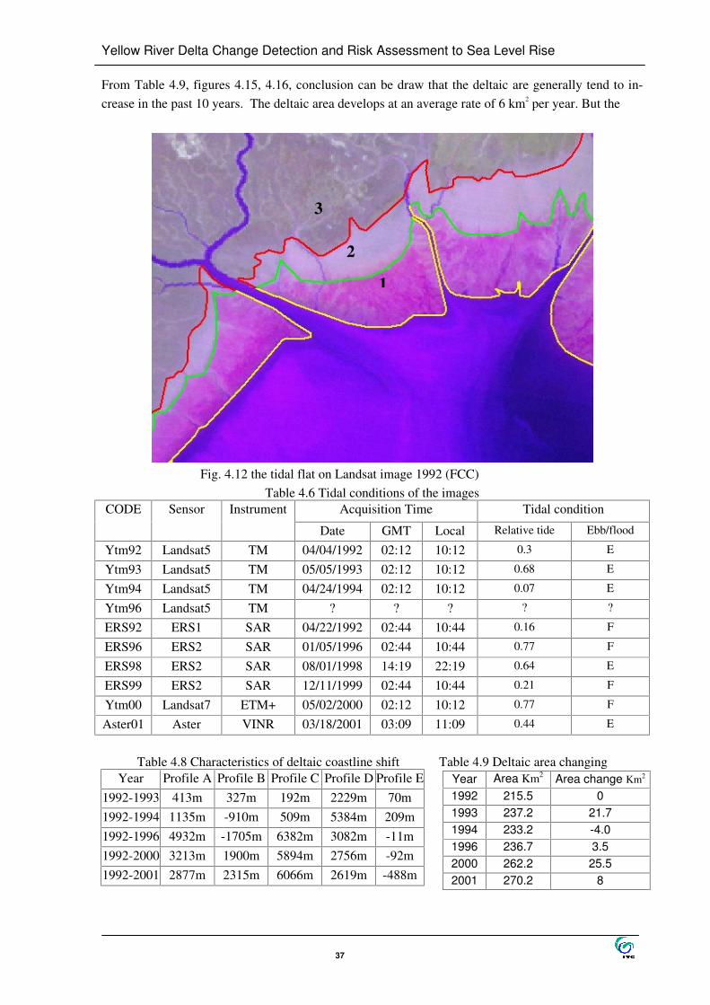
Yellow River Delta Change Detection and Risk Assessment to Sea Level Rise
37
From Table 4.9, figures 4.15, 4.16, conclusion can be draw that the deltaic are generally tend to in-crease in the past 10 years. The deltaic area develops at an average rate of 6 km2 per year. But the
Fig. 4.12 the tidal flat on Landsat image 1992 (FCC)
Table 4.6 Tidal conditions of the images Acquisition Time Tidal condition CODE Sensor Instrument
Date GMT Local Relative tide Ebb/flood
Ytm92 Landsat5 TM 04/04/1992 02:12 10:12 0.3 E
Ytm93 Landsat5 TM 05/05/1993 02:12 10:12 0.68 E
Ytm94 Landsat5 TM 04/24/1994 02:12 10:12 0.07 E
Ytm96 Landsat5 TM ? ? ? ? ?
ERS92 ERS1 SAR 04/22/1992 02:44 10:44 0.16 F
ERS96 ERS2 SAR 01/05/1996 02:44 10:44 0.77 F
ERS98 ERS2 SAR 08/01/1998 14:19 22:19 0.64 E
ERS99 ERS2 SAR 12/11/1999 02:44 10:44 0.21 F
Ytm00 Landsat7 ETM+ 05/02/2000 02:12 10:12 0.77 F
Aster01 Aster VINR 03/18/2001 03:09 11:09 0.44 E
Table 4.8 Characteristics of deltaic coastline shift Table 4.9 Deltaic area changing
Year Profile A Profile B Profile C Profile D Profile E 1992-1993 413m 327m 192m 2229m 70m 1992-1994 1135m -910m 509m 5384m 209m 1992-1996 4932m -1705m 6382m 3082m -11m 1992-2000 3213m 1900m 5894m 2756m -92m 1992-2001 2877m 2315m 6066m 2619m -488m
1
3
2
Year Area Km2 Area change Km2 1992 215.5 0 1993 237.2 21.7 1994 233.2 -4.0 1996 236.7 3.5 2000 262.2 25.5 2001 270.2 8

Yellow River Delta Change Detection and Risk Assessment to Sea Level Rise
38
Fig. 4.13 The mask of study area for coastline change detection on the Landsat image (May.2 2000)
Fig. 4.14 The development of the most active delta on optic image interpretation
Study area
.
. Profile C
Profile E
Profile B
GUDONG
Yellow
River
SEA
BOHAI
LAIZHOU GULF Profile A Profile D
P1
P2

Yellow River Delta Change Detection and Risk Assessment to Sea Level Rise
39
crement varied. As can de seen see in figure 4.16, the increment increased from 1992 to 1993, but from 1993 to 1994, the increment decreased. From 1994 to 2000, the Yellow River delta active part developed in a relatively fast progress. This can be explained by the fact that the Yellow River was artificially diverted from South-East to North-East in 1996. Since 1976 the Yellow River was artifi-cially diverted from the Goukouhe course to the Qinshuigou course. This is the other major diversion. An active sub-delta started to develop. It is about 20 square kilometres on the 2000 image. According to Yang (1995), for the stage of June, 1996-Nov., 1981, the yearly increment averaged 36 km2. It was the most important delta developing stage. During the stage of Nov. 11, 1981- Nov. 1988, the average increment amounted to 27 km2 per year. While from 1998 till April 1994, the deltaic area increased at an average of 2 km2 per year. This figure is less than the increment of 6 km2 per year from 1992 till 2001. Figure 4.16 indicates that there are two periods of increasing trends of delta area. One is from 1992 to 1993; other is from 1996 to 2000. From 1990 to 1992, The Yellow River was occa-sionally in a dry state in which. No more sediment was carried to the sea, Therefore the river mouth siltbar and natural levees suffered from increasing strong erosion. So in 1992 the delta shows a loss of area. But days of dry out in 1993 are fewer 23 days than in 1992 at Huayuankou station. During this stage of 1992-1993, the increment is about 23 km2. Due to artificial diversion in 1996, a new sub-delta started to develop. The relationship between discharge and delta area change will be analysis in section 4.4.1. Instead of a presentation of the coastline length, the 5 profiles were plotted (see figure 4.14). The measurements of the coastline change in profile direction are presented in table 4.8. The curves of the YRD coastline shift along 5 profiles are given in figure 4.17. Based on table 4.8 and figures 4.14 and 4.17, we can conclude that the deltaic boundary expended from 1992 to 1993, along profile A, and in 1994, the head of the Yellow River shifted from south-east to south, the delta developed in south di-rection (see profile D). After that the mouth of the river shifted back again, it is presented well on landsat image 1996. After 1996, the delta receded in the Southeast direction. This is due to the diver-sion of 1996 artificially. Then river changed its channel towards Northeast a new sub-delta was cre-ated and developed. No sediment was carried into the sea through this direction. As can be seen along profile C in figure 4.14, the deltaic boundary extends at an average of 348 m per year. In fact the border extension is 3797 m only in 1996 within a few month after the Yellow River diversion. In pro-file E the coastline is more or less stable. But on the southwest side the coastline varies frequent and the range of the change is more. Along profile B, the border of delta receded from 1993 to 1996, and extended from 1996 to 2001. This indicates that the delta suffered from stronger erosion during the stage of 1993-1996, and inversely sedimentation was strong than the erosion during the stage of 1996-2001 in the southwest zone.
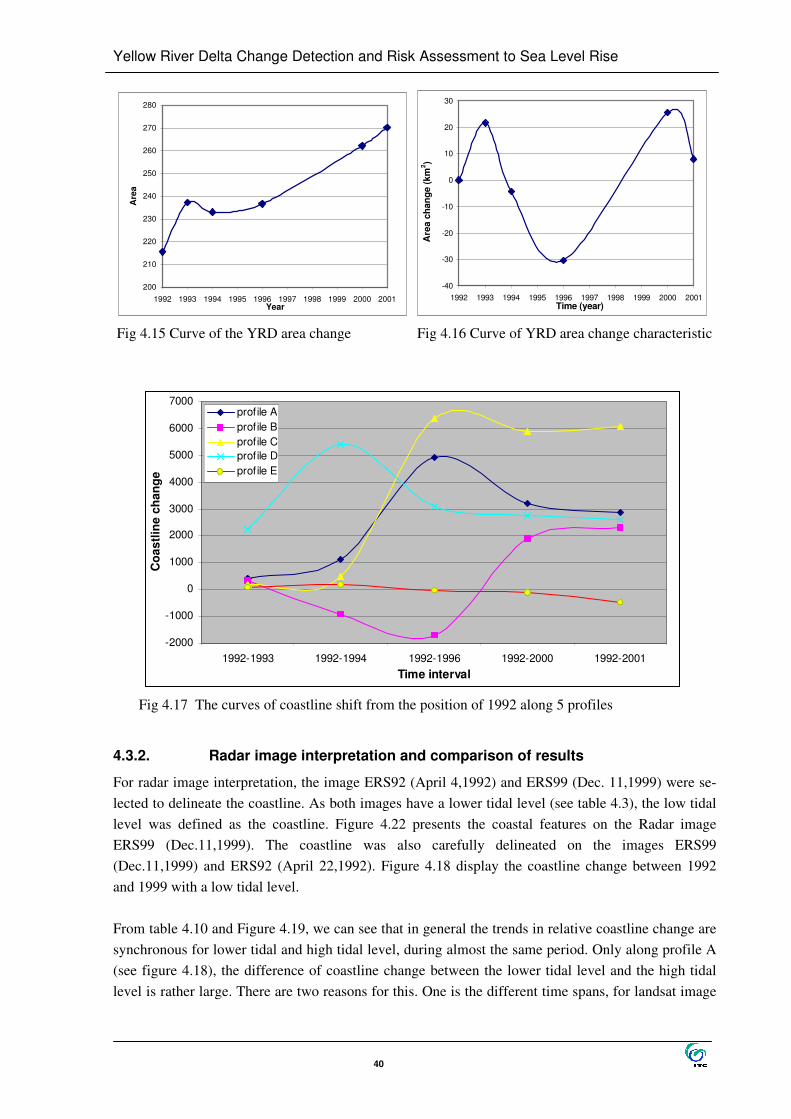
Yellow River Delta Change Detection and Risk Assessment to Sea Level Rise
40
200
210
220
230
240
250
260
270
280
1992 1993 1994 1995 1996 1997 1998 1999 2000 2001Year
Are
a
-40
-30
-20
-10
0
10
20
30
1992 1993 1994 1995 1996 1997 1998 1999 2000 2001Time (year)
Are
a ch
ange
(km
2 )
Fig 4.15 Curve of the YRD area change Fig 4.16 Curve of YRD area change characteristic
-2000
-1000
0
1000
2000
3000
4000
5000
6000
7000
1992-1993 1992-1994 1992-1996 1992-2000 1992-2001Time interval
Coa
stlin
e ch
ange
profile Aprofile Bprofile Cprofile Dprofile E
Fig 4.17 The curves of coastline shift from the position of 1992 along 5 profiles
4.3.2. Radar image interpretation and comparison of results
For radar image interpretation, the image ERS92 (April 4,1992) and ERS99 (Dec. 11,1999) were se-lected to delineate the coastline. As both images have a lower tidal level (see table 4.3), the low tidal level was defined as the coastline. Figure 4.22 presents the coastal features on the Radar image ERS99 (Dec.11,1999). The coastline was also carefully delineated on the images ERS99 (Dec.11,1999) and ERS92 (April 22,1992). Figure 4.18 display the coastline change between 1992 and 1999 with a low tidal level. From table 4.10 and Figure 4.19, we can see that in general the trends in relative coastline change are synchronous for lower tidal and high tidal level, during almost the same period. Only along profile A (see figure 4.18), the difference of coastline change between the lower tidal level and the high tidal level is rather large. There are two reasons for this. One is the different time spans, for landsat image

Yellow River Delta Change Detection and Risk Assessment to Sea Level Rise
41
this is from 1992 to 2000, for ERS from 1992 to 1999. The other is slope along this profile is vary with depth change. Based on the above-described result, the conclusion can be drawn that ERS SAR images can be ap-plied to monitor the coastline change. For the relative stable slope tideland, relative change is ap-proximate using different methods of high tidal level interpretation and low tidal level interpretation.
Table 4.10 The distance comparison of coastline shift between ERS (lower tidal level) and Landsat images (high tidal level)
Profile A Profile B Profile C Profile E ERS
1992-1999 Landsat
1992-2000 ERS
1992-1999 Landsat
1992-2000 ERS
1992-1999 Landsat
1992-2000 ERS
1992-1999 Landsat
1992-2000 2037m 3213m 2184m 1900m 5074m 4932m -462m -92m
Fig. 4.18 The development of the most active delta from Radar image interpretation
Profile B
Profile E
Profile A
Profile C
GUDONG
BOHAI
SEA
LAIZHOU GULF
Yellow River

Yellow River Delta Change Detection and Risk Assessment to Sea Level Rise
42
-500
500
1500
2500
3500
4500
5500
A B C EProfile
Coa
stlin
e sh
ift d
ista
nce
(m)
ers1992-1999Landsat1992-2000
Fig. 4.19 The comparison of coastline shift between approaches (ERS images with low tide and Landsat images with high tide)
4.4. Conclusion and discussions
This section gives a general discussion on the factors that affect the deltaic coastline change. There are many factors controlling the development of the delta. These include hydrologic aspects (river discharge, sediment load, minimum dry period flow and the amount of transported sediment, etc.), marine hydraulic aspects (tides, sea level rise, storm surge, longshore drift, currents, wave action, etc.), geomorphologic and geological aspects, climatic aspects, landuse and human activities (artificial diversion, embankments, pumping of the oil, irrigation, etc.). It is clear that recent human activities have also posed a strong effect on the delta development.
4.4.1. The impacts of the fluvial process
As the marine influence on the development of the delta actions is relatively weak, the present active (sub) delta can be classified as fluvial-dominated delta (Yang, 1995). The general change trends of the river length and deltaic area are synchronous as illustrated in figure 4.20. This indicates that the change of the deltaic area highly depends on the change of the river channel length. Table 4.11 shows the days of dry out of the Yellow River from 1992 to 2001. The logarithm trend line is used to simu-late the data; high correlation is established between delta area and river dry out days (Figure 4.21B), the correlation coefficient is 0.8867. In general, we conclude that the dry out days increase, then the delta recede. But as you see the correlation coefficient of trend line in figure 4.21 (A) is not such a good fit as in figure 4.21 (B). The reason can be explained that the Yellow River channel was changed artificially from southeast to northeast for oil exploitation activities, and a new sub-delta was formed that is growing faster. Even in 1996, the days of dry out is 136 days, the delta area still keep increment.

Yellow River Delta Change Detection and Risk Assessment to Sea Level Rise
43
Table 4.11days of dry out of the Yellow River and its length
Year Area (km2) Length (km) Days of dry out 1992 215.5 22.496 83 1993 237.2 23.21 60 1994 233 26.172 74 1996 236.7 40.08 136
2000 262 37.836 50∗ 2001 270 37.105 52*
(Data source: http://www.hydroinfo.gov.cn/sqnb/1998/98-8.html)
0
5
10
15
20
25
30
35
40
45
1992 1994 1996 1998 2000 2002Time
Leng
th (k
m)
0
50
100
150
200
250
300
Are
a(K
m2 )
Linear (River Length)Linear (Delta Area)
Fig 4.20 The comparison of the deltaic area against river channel length.
A B Fig.4.21 Correlation between dry out days and delta area
4.4.2. The impacts of the marine processes
∗ Dry out days of 2000 and 2001 were estimated approximation by author
y = -95.025Ln(x) + 636.57R2 = 0.8867
200
210
220
230
240
250
260
270
280
40 50 60 70 80 90
River dry out (days/year)
Are
a ch
ange
(km
2 )
y = -32.847Ln(x) + 382.51R2 = 0.3726
200
210
220
230
240
250
260
270
280
40 50 60 70 80 90 100 110 120 130 140 150
River dry out (days/year)
Are
a ch
ange
(km
2 )
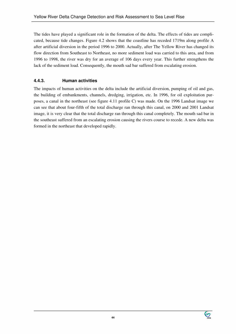
Yellow River Delta Change Detection and Risk Assessment to Sea Level Rise
44
The tides have played a significant role in the formation of the delta. The effects of tides are compli-cated, because tide changes. Figure 4.2 shows that the coastline has receded 1719m along profile A after artificial diversion in the period 1996 to 2000. Actually, after The Yellow River has changed its flow direction from Southeast to Northeast, no more sediment load was carried to this area, and from 1996 to 1998, the river was dry for an average of 106 days every year. This further strengthens the lack of the sediment load. Consequently, the mouth sad bar suffered from escalating erosion.
4.4.3. Human activities
The impacts of human activities on the delta include the artificial diversion, pumping of oil and gas, the building of embankments, channels, dredging, irrigation, etc. In 1996, for oil exploitation pur-poses, a canal in the northeast (see figure 4.11 profile C) was made. On the 1996 Landsat image we can see that about four-fifth of the total discharge ran through this canal, on 2000 and 2001 Landsat image, it is very clear that the total discharge ran through this canal completely. The mouth sad bar in the southeast suffered from an escalating erosion causing the rivers course to recede. A new delta was formed in the northeast that developed rapidly.

Yellow River Delta Change Detection and Risk Assessment to Sea Level Rise
45
Fig. 4.22 Most active Yellow River Delta on Radar image (Dec. 11,1999)
BOHAI
SEA
LAIZHOU GULF
Yellow River
Coastline Tideland
Tidal creek
Yellow River Delta Change Detection and Risk Assessment to Sea Level Rise
46
5. Vulnerability assessment of the YRD to Sea Level Rise-related Storm Surge
This chapter is to assess the flood vulnerability and risk of the YRD to predicted sea level rise, and analysis of the potential impacts of sea level rise on socio-economic attributes of the YRD.
5.1. Conceptual framework
5.1.1. Conceptual framework of vulnerability assessment to sea level rise
Sea level rise and its impacts on coastal zones are the evolving process of global warming. Up to 2100, global mean sea level (MSL) is projected to rise by 9-88 cm (IPCC WGI, 2001). In many sensi-tive deltaic and coastal plains, the range of relative sea level rise will be several times than this global mean value due to local rapid land subsidence. It will result in a series of adverse effects on the eco-environmental evolution and socio- economic development of these areas. Assessing coastal vulner-ability to sea level rise is practised in order to delimit the vulnerable zone, characterize the vulnerabil-ity types and estimate the extent of potential damages of sea level rise on deltaic and coastal plains. It depends not only on the sensitivity of the natural coastal system and the fragility of the socio-economic system to sea level rise, but also on the protection level of the coastal area being defended. The Intergovernmental Panel on Climate Change (IPCC) has made an appeal to all coastal countries to firstly assess coastal vulnerability. In collaboration with experts from various international bodies, in September 1991, the Coastal Zone Management Subgroup (CZMS) published “ The Seven Steps for the Assessment of the Vulnerability of Coastal Areas to Sea Level Rise – A Common Methodology” (Figure 5.1). The vulnerability of coastal areas to sea level rise is not merely the identification of re-sources at risk. The common methodology defines vulnerability of coastal zones as a nation’ s ability to cope with the consequences of acceleration in sea level rise and other coastal impacts of globe cli-mate change. Vulnerability assessment (AV) is an analysis of the scope and severity of the potential effects of acceleration sea level rise (Nicholls, 1995).
The objectives of the methodology are to provide a framework to:
• Identify and assess the physical, ecological, and socio-economic vulnerability to accelerated sea level rise and other coastal impacts of globe climate change;
• Understand how development and other socio-economic factors affect vulnerability; • Clarify how possible responses can mitigate vulnerability, and assess their residual effects; • Evaluate a country’ s capacity for implementing a response within a broad coastal zone
management framework.

Yellow River Delta Change Detection and Risk Assessment to Sea Level Rise
47
Fig 5.1 Seven steps for the assessment of the vulnerability of coastal area to seal level rise Most coastal vulnerability studies focused on a single socio-economic scenario based on today’ s situation. The existing syntheses of impacts of sea level rise consider a 1-m rise in sea level compared to the present situation (IPCC CZMS, 1992; WCC’ 93, 1994; Nicholls, 1995; Bijlsma et al., 1996). At most, six factors are considered, including the use of expert judgement to evaluate factors where quantitative results were not available. The first five factors assume no human response to sea-level rise, while the last one factors consider the consequences of human adaptation. The factors are as fol-lows:
• People affected (the people living in the hazard zone affected by sea-level rise); • People at risk (the average annual number of people flooded by storm surge); • Capital value at loss (the market value of infrastructure which could be lost due to sea-level
rise); • Land at loss (the area of land that would be lost due to sea-level rise); • Wetland at loss (the area of wetland that would be lost due to sea-level rise); • Potential adaptation costs, with an overwhelming emphasis on protection;
The methodology of vulnerability assessment to SLR provided by IPCC mainly focus on Global Vul-nerability assessment and national vulnerability assessment. It has limited knowledge about vulner-
STEP 1
Delineation of case study area and specification of SLR and climate
STEP 2
Delineation of natural system and socio-economic system data
STEP 3
Delineation of relevant development factors
STEP 4
Assessment of physical changes and natural system responses
STEP 5
Formulation of response strategies
STEP 6
Assessment of vulnerability and interpretation of result
STEP 7
Identification of needs and actions
Yellow River Delta Change Detection and Risk Assessment to Sea Level Rise
48
ability to sea level rise at the regional scale (Watson et al., 1998). While there are a number of sub-national and national scale assessments, they have been developed with different methodologies and
goals (http://www.survas.mdx.ac.uk/backgrou.htm)�
5.1.2. Conceptual framework of risk assessment of natural hazard
UNDRO (1991) defines risk as the expected number of lives lost, persons injured, damage to property and disruption of economic activity due to a particular natural phenomenon, and consequently, the product of specific risk and elements at risk. It is by using such as an estimate that well-founded dis-aster mitigation measures can be designed and put into effect. Natural hazard is the probability of occurrence, within a special period of time in given area, of a potentially damaging natural phenomenon. Vulnerability is the degree of loss to a given element at risk, or set of such elements, resulting from the occurrence of a natural phenomenon of a given magnitude, and expressed on a scale from 0 (no damage) to 1 (total damage). Element at risk is the population, buildings and civil engineering works, economic activities, public services, utilities and infrastructure, etc., at risk in a given area. Specific risk (Rs) is the expected degree of loss due to a particular natural phenomenon and as a func-tion of both natural hazard and vulnerability (one element at risk or structural type i.e. a group of con-struction with similar damage performance when exposed to a specific natural hazard involved). For different categories of elements at risk (E) combined, estimation of specific risk is: Rs = V*Val*P Where, Rs is specific Risk Val is the monetary valuation of the elements at risk, which is also indicative of loss. (For casualties, the Val should be replaced by population density). V is vulnerability of the elements at risk, which varies according to the return periods of hazards. P is probability of occurrence of hazard, which indicates the hazard magnitude. Total risk (Rt) is the expected number of lives lost, persons injured, damage to property and disrup-tion of economic activity due to a particular natural phenomenon, and consequently, the product of specific risk and elements at risk (given as probability). Thus: Rt = (E) (Rs) = (E) (H.V) The process of risk assessment:

Yellow River Delta Change Detection and Risk Assessment to Sea Level Rise
49
Hazard assessment is the assessment of a natural hazard itself and it direct effect. Hazard assessment aims: (a) the natural, severity and frequency of hazard; (b) the area likely to be affected; and the time and duration of impact. Vulnerability analysis is the process used to identify vulnerable conditions that are exposed to natural hazard. It includes the physical vulnerability, social vulnerability and economic vulnerability. Risk assessment defines the relationship between the probability of the natural hazard and the ex-pected losses (Kingma, 1997).
5.1.3. Risk assessment of the YRD to SLR related storm surge
Sea level rise will increase risk of flooding and storm damage. In this research work, risk of the YRD was assessed to sea level rise and storm surge. The basic methodology of risk assessment based on concept defined by UNDRO (1991). Historical records of storm surge in the YRD area and the rela-tive sea level rise estimated by IPCC are data sources used to assess the flood risk. Parameters influencing flood damage are water depth and the duration of flood as well as water veloc-ity and sediment load. Flood duration is often a function of flood depth and sediment load is usually related the velocity of the flood water (Smith and Tobin 1979, cited in Smith and Ward 1998). Since most of the mentioned characteristics are difficult to determine or interrelated to other parameters, many approaches use the relationships between flood depth and damage, so called depth-damage function (Martin, 2000). Population, GDP and landuse are three factors considered in this research work. Vulnerability functions state a relationship between flood depth and each factor. This is de-scribed in section 5.3.
5.2. Creation of Database
5.2.1. Creation of a digital elevation model
A Digital Elevation Models (DEM) is a digital representation of a set of elevations. This can be the elevation of the terrain surface (also called Digital Terrain Model), or the altitude of soil-layers, con-tact of soil-rock, water table etc. The DEM map is a basic data layer for the assessment of flood risk. The available elevation data for this study is a contour map of 1971. The estimated relative sea level rise rate in the Yellow River Delta is 8 mm/year and the sea level rise is expected to be 48 cm by the year 2050 (from 1999). A rise in relative sae level of 48cm cm by 2050 is based on the height of the mean sea level in 1999. However, between 1971 and 1978 the relative sea level changes in the YRD are complicated. Two most remarkable facts can be pointed out. The first is the severe seismic activ-ity along the Bohai Sea coast. The second is the effect of the Tangshan earthquake in 1976. According to Ren Mei-e (missing date), from 1952 to 1978 the relative sea level rise rate is 19mm per year. However, from 1978 to 1999, the relative sea level rise data of recent YRD is not available. 8mm/year
Hazard assess-
Vulnerability analysis Damage assessment
Risk assessment

Yellow River Delta Change Detection and Risk Assessment to Sea Level Rise
50
relative sea level rise was taken as an assumption. So, a total of 31.2cm elevation is subtract from ele-vation of The YRD. The DEM map was update to 1999. Figure 5.2 shows the method of generation of DEM
Fig.5.2 Flow chart for the creation of DEM
Fig.5.3.DEM map of the YRD
5.2.2. Prediction of socio-economic factors and flood estimates
Contour map
Scanning and geo-referencing
On screen digitising
Contour interpolation
DEM map
Subtract 30.2 cm

Yellow River Delta Change Detection and Risk Assessment to Sea Level Rise
51
The risks to population, Gross Domestic Products (GDP) and landuse as result of sea level rise and storm surge were analysed. The study area of DongYing city covers five counties consisting of 51 administrative towns. From the statistic annuals of this administration zone, annuals population increasing rate (PIR), GDP increasing rate (GIP) from 1985 to 1990 as well as population and GDP of 1999 were collected from in the Internet (see table 5.1).
Table 5.1 statistic data of PIR and GIP from 1985 to 1999
Year 198
5
198
6 1987 1988 1989 1990 1991 1992 1993 1994 1995
199
6 1997 1999
PIR % 0.55 0.81 0.94 0.88 0.93 1.60 0.85 0.85 0.05 0.34 0.64 0.81 0.81 0.62
GIR % 23.4 9.6 23.1 10.5 1.4 0 14.3 12.8 23 19.1 9.7 7.6 11.2 7.2
Figure 5.4 shows that the rate of population growth is decreasing. The formula of trendline is: Y=-0.08x + 166.88 Based on this increasing rate formula and the population of each town of 1999, the population of each town by 2050 and 2100 were predicted. The calculation were carried out in Excel using the flowing formula year by year P n+1 =P n * (-0.08*n + 166.88) /1000 + Pn
Where, n is the year from 1999 to 2100, Pn is the population of the year n.
y = -0.08x + 166.88
0
2
4
6
8
10
1985 1987 1989 1991 1993 1995 1997 1999 2001Year
Pop
ulat
ion
incr
easi
ng r
ate
%0
(PIR
)
PIRPIR trendline
Fig5.4 The prediction of population increasing rate
For prediction of GDP, given in table 5.1 the GDP increasing rate of each year is not stable and varies considerably. According to the situation of the Chinese national and local economic development, 7.2 % was adopted as the increasing rate of GDP to predict the GDP of each town by 2050 and 2100. The GDP data of 1999 for each town are available, the calculation were carried out in Excel using the flowing formula:
GDP2050 = GDP1999 * (1+0.072) 51 GDP2100 = GDP1999* (1+0.072) 101

Yellow River Delta Change Detection and Risk Assessment to Sea Level Rise
52
For the planning of Dongying administration, the regional integrated landuse development has been mapped. However, the urban areas in this map keep the same size. Obviously, this cannot match the need of urban development. In this study, the expansion of the urban area was taken into considera-tion. Suppose the urban area by 2050 will be double of the present size, and by 2100 it will be gain double of the size of 2050. At the same time, suppose the urban area will grow in a circle. So the urban area in 2050 and 2100 can be predicted based on Area =2πR2. All urban was divided into two
groups: one is the capital city of this region; and main cities. Table 5.2 shows the size of extension of the urban, ∆R will be used to make a distance buffer of the urban maps. It is described in the next sec-
tion.
Table 5.2 the extension prediction of urban area by 2050 and 2100 Main cities Capital city
Year Average area (m2) R (m) ∆R Area (m2) R (m) ∆R
1995 3,001,361 977 0 31,714,200 3177 0 2050 6,002,723 1382 405 63,428,400 4493 1316 2100 12,005,446 1955 573 126,856,800 6356 1863
5.2.3. Generation of thematic maps
• The generation of the administrative map First, the administrative map was generated in order to create the Population density map and the GDP density map. Fig.5.5 shows the flowchart of the creation of the administrative map.
Fig.5.5 the flowchart of creation of administrative map • The generation of the population and GDP density maps
Administrative map of study
Scanning and Geo-referencing
On screen digitising boundary of each town
Creation of town Domain
Polygon operation
Rasterizing
Administrative map in digital format

Yellow River Delta Change Detection and Risk Assessment to Sea Level Rise
53
Based on the administrative map and the population and GDP data predicted in section 5.2.2, the population density map and GDP map were generated. The first the population and GDP data pre-dicted were input to administrative table. By table calculation, the population and GDP density can be calculated using formula population density = population/area and GDP density=GDP/area Table 5.4 shows a part of the calculation result. From this table the population density and GDP density maps were generated using attribute map of raster map operation in ILWIS.
Table 5.4 Calculation of population and GDP density

Yellow River Delta Change Detection and Risk Assessment to Sea Level Rise
54
• The generation of the landuse development map
The landuse source map is taken from the Atlas of The Yellow River Delta, based on the development plan of the local government. As mentioned in section 5.2.2, suppose the urban area by 2050 will have been doubled that of the present area and by 2100 it will have doubled that of 2050. The exten-sion distance was calculated and used to make the map of urban area. The Figure 5.6 is the flowchart of landuse mapping in ILWIS. For the determination of the value of the elements at risk, here only urban, agriculture landuse cate-gory were taken into account to assess the loss or damage in monetary value. For others elements at risk such as natural reserve, flat area, etc., it is difficult to estimate the value in monetary terms. In addition, time was limited to estimate elements at risk per landuse class. However, the natural reserve and tidal flat area are most important parts of Yellow River Delta. The loss of natural reserve and tidal flat in area were estimated. The estimated property value for agriculture, urban area was listed in Table 5.5.
Table 5.5 the monetary value of elements at risk Category Value per hectare (million in YMB) Value per cell (900 m2) in YMB
Urban 12 1,080,000 Agriculture 0.023 20,700
By attributing map of landuse map with columns, the monetary value maps of urban, agriculture and rice were produced.
5.3. Modelling of storm flooding to sea level rise
According to Keith Smith and Roy Ward (1998), more usually, flooding in coastal areas is caused by “ something extra” , over and above the normal tidal and wave conditions. So, coastal and estuarine flooding results, not from the normal regime of waves and tides but from an extra factor, which adds to the height of the sea surface, especially when that addition coincides with high-tide conditions. On open coastlines, a common cause of flooding is the severe meteorological conditions, which produce abnormally high sea levels, known as storm surge. The dangers of storm flood are associated with a number of different parameters, such as: Depth of water: building stability against flotation and foundation failures, flood proofing, and vegetation survival, have different degrees of tolerance to inundation. In each case these can usually be identified and the depth established. Duration: the time of the inundation is of utmost importance since the degree of damage is often re-lated to it. This applies to structural safety, the effect of interruption in communications, industrial activity and public services, and agriculture.

Yellow River Delta Change Detection and Risk Assessment to Sea Level Rise
55
Velocity: high velocity of flow creates high erosive forces and hydrodynamic pressure. These fea-tures often result in complete or partial failure of structures by creating instability or destroying foun-dation support. Fig5.6 flowchart of the procedure to make the landuse development map in ILWIS
Creation of Landuse development map
Scanning and Geo-referencing
On screen digitising boundary of each landuse unit
Creation of Landuse Domain
Polygon operation
Rasterizing
Landuse map in digital format
Landuse development map
Extraction of urban area Capitalcity:=iff(landuse="capital city","capital city",?) Maincity:=iff(landuse="main city","Main city",?)
Distance calculate: Landuse2050: main cities D=405m; Capital city D=1316m Landuse2100: main cities D=573m; Capital city D=1863m
Extension map of urban in 2050, 2100
Map glue operation
Landuse development map in 2050, 2100
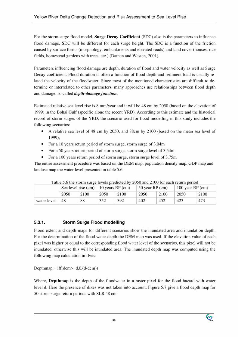
Yellow River Delta Change Detection and Risk Assessment to Sea Level Rise
56
For the storm surge flood model, Surge Decay Coefficient (SDC) also is the parameters to influence flood damage. SDC will be different for each surge height. The SDC is a function of the friction caused by surface forms (morphology, embankments and elevated roads) and land cover (houses, rice fields, homestead gardens with trees, etc.) (Damen and Westen, 2001). Parameters influencing flood damage are depth, duration of flood and water velocity as well as Surge Decay coefficient. Flood duration is often a function of flood depth and sediment load is usually re-lated the velocity of the floodwater. Since most of the mentioned characteristics are difficult to de-termine or interrelated to other parameters, many approaches use relationships between flood depth and damage, so called depth-damage function. Estimated relative sea level rise is 8 mm/year and it will be 48 cm by 2050 (based on the elevation of 1999) in the Bohai Gulf (specific alone the recent YRD). According to this estimate and the historical record of storm surges of the YRD, the scenario used for flood modelling in this study includes the following scenarios:
• A relative sea level of 48 cm by 2050, and 88cm by 2100 (based on the mean sea level of 1999);
• For a 10 years return period of storm surge, storm surge of 3.04m • For a 50 years return period of storm surge, storm surge level of 3.54m • For a 100 years return period of storm surge, storm surge level of 3.75m
The entire assessment procedure was based on the DEM map, population density map, GDP map and landuse map the water level presented in table 5.6.
Table 5.6 the storm surge levels predicted by 2050 and 2100 for each return period Sea level rise (cm) 10 years RP (cm) 50 year RP (cm) 100 year RP (cm) 2050 2100 2050 2100 2050 2100 2050 2100
water level 48 88 352 392 402 452 423 473
5.3.1. Storm Surge Flood modelling
Flood extent and depth maps for different scenarios show the inundated area and inundation depth. For the determination of the flood water depth the DEM map was used. If the elevation value of each pixel was higher or equal to the corresponding flood water level of the scenarios, this pixel will not be inundated, otherwise this will be inundated area. The inundated depth map was computed using the following map calculation in Ilwis: Depthmap:= iff(dem>=d,0,(d-dem)) Where, Depthmap is the depth of the floodwater in a raster pixel for the flood hazard with water level d. Here the presence of dikes was not taken into account. Figure 5.7 give a flood depth map for 50 storm surge return periods with SLR 48 cm
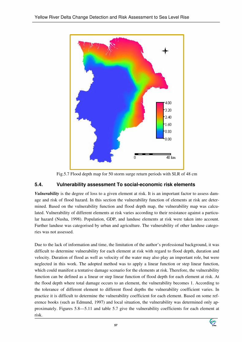
Yellow River Delta Change Detection and Risk Assessment to Sea Level Rise
57
Fig.5.7 Flood depth map for 50 storm surge return periods with SLR of 48 cm
5.4. Vulnerability assessment To social-economic risk elements
Vulnerability is the degree of loss to a given element at risk. It is an important factor to assess dam-age and risk of flood hazard. In this section the vulnerability function of elements at risk are deter-mined. Based on the vulnerability function and flood depth map, the vulnerability map was calcu-lated. Vulnerability of different elements at risk varies according to their resistance against a particu-lar hazard (Nusha, 1998). Population, GDP, and landuse elements at risk were taken into account. Further landuse was categorised by urban and agriculture. The vulnerability of other landuse catego-ries was not assessed. Due to the lack of information and time, the limitation of the author’ s professional background, it was difficult to determine vulnerability for each element at risk with regard to flood depth, duration and velocity. Duration of flood as well as velocity of the water may also play an important role, but were neglected in this work. The adopted method was to apply a linear function or step linear function, which could manifest a tentative damage scenario for the elements at risk. Therefore, the vulnerability function can be defined as a linear or step linear function of flood depth for each element at risk. At the flood depth where total damage occurs to an element, the vulnerability becomes 1. According to the tolerance of different element to different flood depths the vulnerability coefficient varies. In practice it is difficult to determine the vulnerability coefficient for each element. Based on some ref-erence books (such as Edmund, 1997) and local situation, the vulnerability was determined only ap-proximately. Figures 5.8—5.11 and table 5.7 give the vulnerability coefficients for each element at risk.
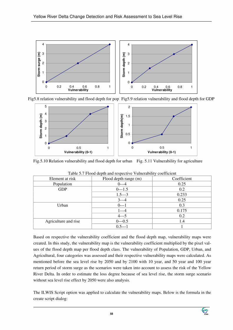
Yellow River Delta Change Detection and Risk Assessment to Sea Level Rise
58
0
1
2
3
4
0 0.2 0.4 0.6 0.8 1Vulnerability
Sto
rm s
urge
(m)
0
1
2
3
4
0 0.2 0.4 0.6 0.8 1Vulnerability
Sto
rm d
epth
(m)
Fig5.8 relation vulnerability and flood depth for pop Fig5.9 relation vulnerability and flood depth for GDP
0
1
2
3
4
5
0 0.5 1Vulnerability (0-1)
Sto
rm d
epth
(m)
0
0.5
1
1.5
2
0 0.5 1Vulnerability (0-1)
Sto
rm d
epth
(m)
Fig.5.10 Relation vulnerability and flood depth for urban Fig. 5.11 Vulnerability for agriculture
Table 5.7 Flood depth and respective Vulnerability coefficient Element at risk Flood depth range (m) Coefficient
Population 0---4 0.25 0—1.5 0.2 1.5---3 0.233
GDP
3---4 0.25 0---1 0.3 1---4 0.175
Urban
4---5 0.2 0---0.5 1.4 Agriculture and rise 0.5---1 1
Based on respective the vulnerability coefficient and the flood depth map, vulnerability maps were created. In this study, the vulnerability map is the vulnerability coefficient multiplied by the pixel val-ues of the flood depth map per flood depth class. The vulnerability of Population, GDP, Urban, and Agricultural, four categories was assessed and their respective vulnerability maps were calculated. As mentioned before the sea level rise by 2050 and by 2100 with 10 year, and 50 year and 100 year return period of storm surge as the scenarios were taken into account to assess the risk of the Yellow River Delta. In order to estimate the loss degree because of sea level rise, the storm surge scenario without sea level rise effect by 2050 were also analysis. The ILWIS Script option was applied to calculate the vulnerability maps. Below is the formula in the create script dialog:

Yellow River Delta Change Detection and Risk Assessment to Sea Level Rise
59
For Population vulnerability map, %1:= iff(%2=0,0,iff(%2>4,1,0.25*%2)) For GDP vulnerability map, %3:=iff(%2=0,0,iff(%2<=1.5,0.2*%2,iff(%2<=3,0.23*%2,iff(%2<=4,%2*0.25,1)))) For Urban vulnerability map, %4:=iff(%2=0,0,iff(%2<=1,0.3*%2,iff(%2<=4,0.175*%2,iff(%2<=5,%2*0.2,1)))) For agricultural vulnerability map: %5:=iff(%2=0,0,iff(%2<=0.5,1*%2,iff(%2<=1.5,0.47*%2,iff(%2<=2,%2*0.5,1)))) Where, 1% indicates the population vulnerability maps of each scenario; 2% indicates the flood depth map maps of each scenario; 3% indicates the GDP vulnerability maps of each scenario, 4% indicates the agriculture vulnerability maps of each scenario, 5% indicates the urban vulnerability maps of each scenario, 1%: Vp2050r10, Vp2050r50, Vp2050r100, Vp2100r10, Vp2100r50, Vp2100r100, Vp2050r10w, Vp2050r50w, Vp2050r100w; %2: Dp2050r10, Dp2050r50, Dp2050r100, Dp2100r10, Dp2100r50, Dp2100r100, Dp2050r10w, Dp2050r50w, Dp2050r100w; %3: Vg2050r10, Vg2050r50, Vg2050r100, Vg2100r10, Vg2100r50, Vg2100r100, Vg2050r10w, Vg2050r50w, Vg2050r100w; %4: Vu2050r10, Vu2050r50, Vu2050r100, Vu2100r10, Vu2100r50, Vu2100r100, Vu2050r10w, Vu2050r50w, Vu2050r100w;

Yellow River Delta Change Detection and Risk Assessment to Sea Level Rise
60
%5: Va2050r10, Va2050r50, Va2050r100, Va2100r10, Va2100r50, Va2100r100, Va2050r10w, Va2050r50w, Va2050r100w; For example, Vp2050r10 indicates the vulnerability map of population for 10 year return period storm surge by 2050.And the file name with “ w” is without sea level rise condition. The result map produces vulnerability values ranging from 0 to 1.
5.5. Damage and loss assessment
5.5.1. Casualties and loss of GDP assessment
The number of casualties was calculated for each flooding scenario by multiplying the population vulnerability map with the predicted population density map (see section 5.2.2. and 5.2.3). The loss of GDP was calculated separately for each flooding scenario by multiplying the vulnerability map with the GDP density map (see section 5.2.2 and 5.2.3). The estimated the number of casualties and GDP loss were given in the table 5.8.
Table 5.8 the number of casualties and GDP loss for each flooding scenario 2050 without SLR 2050 with 48cm SLR 2100 with 88cm SLR Category
10 R 50 R 100 R 10 R 50 R 100 R 10 R 50 R 100 R
Casualties 54,974 80,941 94,489 79,640 114,709 132,199 114,709 126,936 186,392
%Total pop∗∗ 4.3 6.3 7.3 4.4 8.9 10.3 8.9 9.8 14.5 GDP (million)∗ 1639 2491 2932 2442 3580 4159 3580 5206 6056 %Total GDP 1.5 2.3 2.8 2.3 3.4 3.9 3.4 4.9 5.7
The table 5.8 indicates the casualties and GDP loss estimated for each scenario. Casualties estimated amounts to 80,941 people for 50 years return period storm surge without considering sea level rise by 2050 and 114,709 people by considering sea level rise. This result demonstrates the more than 2.6% increase in casualties by considering a sea level rise of 48cm by 2050 for a 50 return period storm surge. In addition, under the same situation 2491 million losses of GDP without considering sea level rise and 3580 million losses with considering sea level rise. The more than 1% increases in the loss of GDP due to sea level rise.
5.5.2. Assessment of the losses of urban and agriculture
Damage was calculated separately for each flood scenario by multiplying the vulnerability layers with the value layers (see section 5.2.2 and 5.2.3). The estimated loss of urban and agriculture are summa-rised in table 5.9. The total damage is subdivided into damage for urban area and agricultural land. Under the same return period, with a 48cm increase of sea level, the damage of urban and agriculture
∗∗ The percent of casualties against total population ∗ In Chinese money (YMB), 1$=8.27 YMB

Yellow River Delta Change Detection and Risk Assessment to Sea Level Rise
61
are increasing about by 96% (10-years storm surge by 2050), about 136% (50-years storm surge by 2050) and about 129% (100-years storm surge by 2050).
Table 5.9 the losses of urban and agriculture for each flooding scenario (million in RMB) 2050 without SLR 2050 with 48cm SLR 2100 with 88cm SLR Category
10 R 50 R 100 R 10 R 50 R 100 R 10 R 50 R 100 R Urban 10.37 21.06 29.94 20.37 50.56 68.66 41.87 97.26 117.71
Agriculture 45.02 91.71 112.10 89.66 141.17 169.61 130.02 216.00 251.03 Total 55.39 112.77 142.04 110.03 191.73 238.27 173.89 313.26 368.74
5.5.3. Assessment of the loss of natural reserve and tidal flat area
As important natural environment factors, the natural reserve and tidal flat loss were estimated. As it is difficult to estimate the economic value of natural reserve and tidal flat, and the ecological value of them is far beyond its economic value, here the area loss of natural reserve and tidal flat only were estimated. The effected area was calculated based on the landuse map and flooding (extent) depth map. The table 5.10 indicates the completely loss area of the natural reserve and tidal flat resulted in sea level rise 48 cm by 2050 and 88 cm by 2100. Table 5.11 shows the effected area of the natural reserve and tidal flat area for each flooding scenario.
Table 5.10 the lost area of the natural reserve and tidal flat for 48 cm and 88 cm SLR scenario Categories SLR 48 cm by 2050 SLR 88 cm by 2100
Natural reserve (Km2) 266 461 % of total natural reserve 25% 44%
Tidal flat (Km2) 98 276 % of total tidal flat 19% 55%
Table 5.10 shows that 266 km2 natural reserve, which is 25% of the total area, will be lost by 2050; and 461 km2, which occupies 44% of total area, will be lost by 2100. The loss of tidal flat area is also critical. 19% of the tidal flat area will be lost by 2050 and so do 55% of the tidal flat by 2100. From table 5.11, we can see the total 502 km2 tidal flat and almost natural reserve area were estimated to be effected even with 10 years return period storm without impact of sea level rise.
Table 5.11 the effected area of the natural reserve and tidal flat for each flooding scenario 2050 without SLR 2050 with 48cm SLR 2100 with 88cm SLR
Category 10 R 50 R 100 R 10 R 50 R 10 R 10 R 50 R 100 R
Total Area (Km2)
Tidal flat (Km2) 502 502 502 502 502 502 502 502 502 502 Natural reserve (Km2) 974 986 992 986 998 1003 996 1010 1015 1046 % Total natural reserve 92.7 94.2 94.8 94.2 95.4 95.8 95.2 96.5 97.0

Yellow River Delta Change Detection and Risk Assessment to Sea Level Rise
62
5.6. Risk assessment
5.6.1. Risk zonation mapping for population and GDP
In this study, scenarios: • A sea level rise of 48 cm for a 50-years and 100-yeras return period by 2050; • Without sea level rise for a 50-years return period by 2050
are considered to create risk zonation maps. The risk of the population for each flooding scenario was calculated based on formula: Risk=(Probability of occurrence)*(Vulnerability of population)*(Population density) (Damen and Westen, 2001) The risk of the GDP element for each flooding scenario was calculated based on formula: Risk = =(Probability of occurrence)*(Vulnerability of GDP)*(GDP density) The flowing flow chart elaborates the step of population risk zonation mapping:
Fig.5.15 the flowchart of population risk zonation mapping Population Risk zonation map density slicing: In the population zonation map for each scenario the study area was classified into four risk zones according to the severity of damage. No Risk Zone: There are no casualties in this area. The critical storm surge cannot cause any kind of loss of life. Low Risk Zone: Pixels with values between 0—0.006 were defined as the low risk zone with 1-7 casualties per square kilometre (pixel size is 30*30m)
Formula: Rsp = population Vulnerability *Population density *RP Rsg = GDP Vulnerability *GDP density *RP
Population (GDP) Risk Maps
Density Slicing
Risk Zonation Map (high, medium,

Yellow River Delta Change Detection and Risk Assessment to Sea Level Rise
63
Moderate Risk Zone: Pixels with values between 0.006-0.012 were defined as the medium risk zone with 7-13 casualties per square kilometre (pixel size is 30*30m) High Risk Zone: Pixels with values between 0.012-1 were defined as the medium risk zone with more 13 casualties per square kilometre (pixel size is 30*30m) Figure 5.16,5.17 and 5.18 show the population risk zonation maps. The risk map for a 50-years return period with a 48cm SLR, has an area of 845 km2 at medium risk, this is about 1.5 times that of the population at medium risk for a 50-years period without considering SLR. For the high risk zonation, it is 1.6 times. GDP Risk zonation map density slicing: In the GDP zonation map for each scenario the study area was classified into four risk zones accord-ing to the severity of damage. No Risk Zone: There are no GDP losses in this area. The critical storm surge cannot cause any kind of loss of GDP. Low Risk Zone: Pixels with values between 0—0.00016 were defined as low risk area with 0-0.17 million (in RMB) GDP loss per square kilometer ( pixel size is 30*30m) Moderate Risk Zone: Pixels with values between 0.00016-0.00032 were defined as the medium risk area with 0.17-0.34 million (in RMB) GDP loss per square kilometer ( pixel size is 30*30m) High Risk Zone: Pixels with values between 0.00032-0.02 were defined as the medium risk area with 0.34-22 million (in RMB) GDP loss per square kilometer ( pixel size is 30*30m) Figure 5.19 and 5.20 and 5.21 show the GDP risk zonation maps.

Yellow River Delta Change Detection and Risk Assessment to Sea Level Rise
64
Fig. 5.16 Risk map of POP∗ for 50 RP∗∗ without SLR Fig. 5.17 Risk map of POP for 50 RP with SLR 48 cm
Fig. 5.18 Risk map of POP for 100 RP with SLR 48cm Fig. 5.19 Risk map of GDP for 50 RP without SLR
Fig. 5.20 Risk map of GDP for 50 RP with SLR 48 cm Fig. 5.21 Risk map of GDP for 100 RP with SLR 48 cm
5.6.2. Overall annual risk for landuse
Based on the estimated damage of agriculture and urban as well as the return period considered, the annual risks were calculated for each of the sea level rise scenarios. Table 5.12, 5.13, and 5.14 indi-cate that the lower magnitude cause more damage over a long period than one large storm event. Fig-ure 5.22, 5.23, 5.24 shows the loss probability for each scenario.
∗ Population ∗∗ Return Period
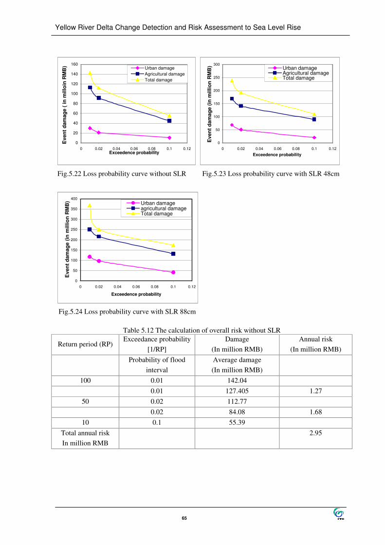
Yellow River Delta Change Detection and Risk Assessment to Sea Level Rise
65
0
20
40
60
80
100
120
140
160
0 0.02 0.04 0.06 0.08 0.1 0.12Exceedence probability
Eve
nt d
amag
e ( i
n m
illoi
n R
MB
) Urban damageAgricultural damageTotal damage
0
50
100
150
200
250
300
0 0.02 0.04 0.06 0.08 0.1 0.12
Exceedence probability
Eve
nt d
amag
e (in
mill
ion
RM
B) Urban damage
Agricultural damageTotal damage
Fig.5.22 Loss probability curve without SLR Fig.5.23 Loss probability curve with SLR 48cm
0
50
100
150
200
250
300
350
400
0 0.02 0.04 0.06 0.08 0.1 0.12
Exceedence probability
Eve
nt d
amag
e (in
mill
ion
RM
B) Urban damage
agricultural damageTotal damage
Fig.5.24 Loss probability curve with SLR 88cm
Table 5.12 The calculation of overall risk without SLR
Return period (RP) Exceedance probability
[1/RP] Damage
(In million RMB) Annual risk
(In million RMB)
Probability of flood
interval Average damage (In million RMB)
100 0.01 142.04 0.01 127.405 1.27
50 0.02 112.77 0.02 84.08 1.68
10 0.1 55.39 Total annual risk In million RMB
2.95

Yellow River Delta Change Detection and Risk Assessment to Sea Level Rise
66
Table 5.13 The calculation of overall risk with SLR 48cm
Return period (RP) Exceedance probability
[1/RP] Damage
(In million RMB) Annual risk
(In million RMB)
Probability of flood
interval Average damage (In million RMB)
100 0.01 238.27 0.01 215.00 2.15
50 0.02 191.73 0.02 150.98 3.02
10 0.1 110.03 Total annual risk In million RMB
5.17
Table 5.14 The calculation of overall risk with SLR 88cm
Return period (RP) Exceedance probability
[1/RP] Damage
(In million RMB) Annual risk
(In million RMB)
Probability of flood
interval Average damage (In million RMB)
100 0.01 368.74 0.01 341.00 3.14
50 0.02 313.26 0.02 243.58 4.87
10 0.1 173.89 Total annual risk (In million RMB)
8.01
5.7. Conclusion
Geographic information system is an operational and useful tool to assess potential sea level rise and storm surge risk. This case study produced quantitative data related to the damage of the Yellow River Delta to an accelerated sea level rise and storm surge. Estimated relative sea level rise rate in the Yellow River Delta is 8 mm/year and the sea level rise will be 48 cm by the year 2050. This study took into account three sea level rise scenarios i.e. without sea level rise and sea level rise 48 cm by 2050, sea level rise 88 cm by 2100. Three storm return period of 10 years, 50 years and 100 years were preformatted. This assessment showed that the relative sea level rise will increase the critical damage with respect to the number of casualties. Based on the estimated casualties for each scenario, the casualties by sea level rise 48cm can increase by 2.6% for a 50 years storm return period by the year 2050. The number

Yellow River Delta Change Detection and Risk Assessment to Sea Level Rise
67
of casualties is 186,392 people by a sea level rise 88cm and 100 years return period storm surge in 2100, which is 14.5% of total population in this region. As for the capital value at loss, the study indicates that the loss of GDP would increase more than 1.1% by a sea level rise 48 cm than without sea level rise for a 50 years return period in 2050. The estimated value loss of urban and agriculture can rise 225% because of a relative sea level rise 48 cm than without sea level rise for 10 years return period in 2050. For tidal land and natural reserve, 266 km2 natural reserve, which is 25% of the total area, will be lost by 2050; and 461 km2, which occupies 44% of total area, will be lost by 2100. The loss of tidal flat area is also critical. 19% of the tidal flat area will be lost by 2050 and so does 55% of the tidal flat by 2100.

Yellow River Delta Change Detection and Risk Assessment to Sea Level Rise
68
6. Conclusion and Recommendation
This study has two objectives. One is to explore the applicability of satellite image in the context of a GIS for the monitoring of the coastline change of the most active Yellow River Delta. The second aim is to deal with risk assessment of the Yellow River Delta to sea level rise related to storm surge apply-ing GIS.
6.1. Conclusion and recommendation for coastline change detection
6.1.1. Conclusion
1. For the images with the same tidal level, image differencing and image overlaying based on post-classification images are very useful and fast techniques to monitor the coastline change. Due to tidal effect, for coastal water and land classification, it is always difficult to identify whether the classified coastline represents the low tidal line, high tidal line or occurring between the two, those two methods have a certain limitation. Image fusion, one of the techniques for change detection, is easy to perform and directly display. Nevertheless, it is difficult to interpret and measure result. 2. For the interpretation and on-screen digitising, the high tidal line defined as the coastline to detect the coastline change is more practical and accurate under tidal level and tideland slop data are not available. Even so, but more attention has to been paid on coastline interpretation. Due to tidal change, ocean wave movement, beach gentle slope, soil and air moisture, water quality, water sub-stratum, habitats, Inaccuracies are caused by those influencing factors. 3. Generally, the area and river channel length of most active YRD tend to increase. A new delta was produced after diversion of the Yellow River artificially in 1996. China government has succeeded in the Yellow River water management project since 1999. This reduces time of no discharge of the Yel-low River and further enhanced the growing rate of the YRD in past 10 years. � 4. The erosion is stronger along northeast coastline except the new delta produced by artificial diver-sion and inverse along the southwest coastline. This results from the impacts of the marine processes; the tides and sea wave have played a significant role in an erosion of delta. 5. Human activities play important role on the coastline change of the YRD. The impacts of human activities on the delta may include the artificial diversion, pumping of the ground fluids, the building of embankments, channels, dredging, irrigation, etc. In 1996, for the oil exploitation purpose, the channel was diverted artificially and a new sub-delta was produced.

Yellow River Delta Change Detection and Risk Assessment to Sea Level Rise
69
6.1.2. Recommendation
1. Considering the high degree of uncertainty of the coastal features mapping, a high accuracy correc-tion of tidal and other marine parameters effects on the coastline should be paid a special attention. 2. The application of RS and GIS to monitor the coastline change should be carried out jointly with routine observatory work in order to improve our understanding of the nature of change.
6.2. Conclusion and recommendation for risk assessment
6.2.1. Conclusion for risk assessment
Geographic information system is an available and very useful tool to assess potential sea level rise and storm surge risk. This case study have produced quantitative data related to the damage of the Yellow River Delta to an accelerated sea level rise and storm surge. According to IPCC (1999), the estimated relative sea level rise rate in the Yellow River Delta is 8 mm/year and the sea level rise will be 48 cm by the year 2050. This study took into account three sea level rise scenarios i.e. without sea level rise and sea level rise of 48 cm by 2050, and sea level rise of 88 cm by 2100. Three storm return period of 10 years, 50 years and 100 years were taken consideration. 1. It appeared that the sea level rise would enhance the critical damage with respect to the number of casualties. Based on the estimated casualties for each scenario, the casualties by sea level rise can be increase 2.6% for 50 years storm return period by 2050. The number of casualties will reach 186,392 people, which is 14.5% of total population in this region by sea level rise related with 100 years re-turn period storm in 2100. 2. As for the capital value at loss, this study indicated that the loss of GDP would increase more than 1.1% by a 48cm sea level rise than without sea level rise for 50 years return period in 2050. The esti-mated value loss of urban and agriculture can rise 225% because of sea level rise for 10 years return period in 2050. 3. For tidal land and natural reserve, 266 km2 natural reserve, which is 25% of the total area, will be lost by 2050 with a 48cm relative sea level rise; and 461 km2, which occupies 44% of total area, will be lost by 2100 with a 88cm relative sea level rise. The loss of tidal flat area is also critical. The 19% of the tidal flat area will be lost by 2050 and so does 55% of the tidal flat by 2100.
6.2.2. Recommendation
Coastal risk to enhanced sea level rise and storm surge depends on not only the sensitivity of natural coastal system and the frangibility of the socio-economic factors, but also on the protection measure to be taken. As estimated damage of the Yellow River Delta is critical, the protection measures have to be carried out to mitigate the loss against sea level rise and storm surge. The local government

Yellow River Delta Change Detection and Risk Assessment to Sea Level Rise
70
must decide for themselves how they would ultimately respond to a rise in sea level relative with storm surge, and make at least some tentative decision fairly soon. In this study the damage were estimated by not considering the dike protection. In fact the existing dike still can play the role to protect this area, how much loss can be reduced if the dike remain exis-tent level. How high dike should be reinforced? And how much it should cost? This is very interesting topic also will be very useful for this region to make decision on cope with sea level rise and storm surge. Because some data were not available or came from the Internet, this study is only a crude assessment of coastal risk to sea level rise relative storm surge. As a test of the method, we assess the coastal damage and risk on a map scale of 1:600,000. Obviously, this scale and its resulting maps do not match with practical application and the reliability is relatively low. Following elements at risk can be further assessed: the loss of coastal tidal flat by inundation, intensi-fied erosion and reduced accretion; potential soil salinization caused by changing groundwater flow pattern in the coastal aquifers and extended seawater intrusion into open river mouths; and enlarge-ment of the endangered area by exacerbating storm surge hazards. The flooding modelling is associated with a number of different parameters, main parameters: depth of water; duration of inundation; high velocity of flow. Due to impacts of surface relief, vegetation, and infrastructure, storm surge depth decreases inland. This is the so-called Surge Decay Coefficient (SDC). Due to limitation of time and data, those factors haven’ t been taken into account in this as-sessment. Prediction of population increasing and economic development is crude and uncertain due to the ef-fects of some uncertain factors. The result of this study only gives the approximately risk assessment to sea level rise and storm surge.
Yellow River Delta Change Detection and Risk Assessment to Sea Level Rise
71
Reference: Bijlsma,L.et al., 1996. Coastal zone and small islands. In: R.T. Watson, M.C. Zinyowera, and R.H. Moss (eds.) Climate Change 1995: Impacts, Adaptations, and Mitigation of Climate Change: Scien-tific-Technical Analyses. Contribution of Working Group II to the Second Assessment Report of the Intergovernmental Panel on Climate Change. Cambridge University Press, 289-324. IPCC CZMS, 1992. Global Climate Change and the Rising Challenge of the Sea. Report of the Coastal Zone Management Subgroup. IPCC Response Strategies Working Group, Rijkswaterstaat, the Hague. Nicholls, R.J. 1995. Synthesis of Vulnerability Analysis Studies. In: WCC’93, Preparing to Meet the Coastal Challenges of the 21st Century. Proceedings, World Coast Conference, Noordwijk, Nov. 1993, Rijkswaterstaat, The Hague, p.181-216. WCC’93 1994. Preparing to Meet the Coastal Challenges of the 21st Century. World Coast Confer-ence Report, Noordwijk, Nov. 1993, Rijkswaterstaat, The Hague. Ren Mei-e (????) Effect of sea level rise and land subsidence on the Yellow River Delta A prelimi-nary study Keith Smith and Roy Ward. 1998. Floods Physical Processes and Human Impacts Yang, 1995, Monitoring morphodynamic aspects of the present Huanghe River Delta, China. An ap-proach of the integration of satellite remote sensing and geoinformatic systems. Pang, J., 1994, Fluvial process on the Huanghe Delta and its influence on lower reaches, in: Chinese Academy of Sciences (edt.). The influences of sea level rise on the Deltas of China and Measure-ments, 147-157, Science Press, Beijing, China. Mei-e Ren and H.jesse Walker 1998, Environmental consequences of human activity on the yellow river and its delta, China Van Veen. , 1997 synthetic aperture radar, principles, applications and speckle reduction P. Vass and B. Battrick. 1995, ESA ERS-1 product specification: general information 1. Synthetic aperture radar image mode. 2. Synthetic aperture radar wave mode. 3. Wind scatterometer. 4.Radar altimeter 5. Orbit 6. Gravity field models. B. Battrick. ,1992, ERS-1 user handbook Van der sanden, J.J. 1997, radar remote sensing to support tropical forest management
Yellow River Delta Change Detection and Risk Assessment to Sea Level Rise
72
Nusha 1998, Impact study and economic assessment of flood control measures and flood risk model-ling using integrated GIS and remote sensing techniques Watson, R.T., Zinyowera, M.C. & Moss, R.H. (eds) 1998. The Regional Impacts of Climate Change: An As-sessment of Vulnerability. Cambridge University Press, Cambridge Martin Schlerf, 2000, Flood hazard modelling and risk assessment of Tieler-Culemborgerwaard Pol-der, Netherlands Edmund penning, 1997, The benefits of flood alleviation: A manual of assessment techniques M.C.J.Damen and C.J.Van Westen, 2001, Modeling Cyclone Hazard in Bangladesh J.L.Van Genderen and C.Pohl, 1994, Image fusion optical and microwave satellite data for earth sciences applications Van der Sanden, 1997, Radar remote sensing to support tropical forest management van Gelder, van den berg, G. Chenge and C.Xue, 1994, Overbank and channelfill deposits of the modern Yellow River Delta, Sedimentary Geology. Cheng, 1991, Modern sedimentalogical process and model of the Yellow River Delta.