The Air Distribution in Buildings with Combined Natural and Mechanical Ventilation GUNNAR ÅHLANDER

Licentiate Thesis Division of Building Services Engineering Department of Civil and Architectural Engineering KTH Royal Institute of Technology SE-100 44 STOCKHOLM, SWEDEN May 2004

ISSN 0284 – 141X ISRN KTH/IT/M--61--SE

Preface During my studies at the Royal Institute of Technology, and during my years as a consulting engineer, I had never a thought of any other possible ventilation solution than the use of mechanical ventilation. The only choice was between supply-exhaust and exhaust ventilation. In the beginning of the 90’s, my family and me bought an old one family house without any trace of a designed ventilation system. To my big surprise I found the climate in this house very pleasant. This was the catalyst for my thoughts about how to integrate the best properties of two worlds, natural and mechanical ventilation. This licentiate thesis is a result of these thoughts. I wish to thank my supervisor, Professor Tor-Göran Malmström, for his encouraging support during the years. For the first paper, and the chapter “An example of one zone ventilation”, I also wish to thank Professor Folke Peterson for supervising. Finally I wish to thank my family for all their support. This work has been partly financed by The European Regional Development Fund. Gunnar Åhlander Nyköping, April 2004

Summary This work describes result from both measurements on a number of one family houses, an analytical study of a one-zone model and multi zone studies of a two storey building. The simulations are performed as both parametric studies, with combined values of outside temperature, wind velocity and wind direction, and whole year simulations. For the latter, a climate file for the northern Swedish city Östersund is used. The results, for the whole year simulations, are presented as ventilation availabilities. The ventilation availability is defined as the relative time of the heating season during which a specified airflow is exceeded. This specified airflow may e.g. be a Building Code requirement if such exists. The influence of different measures, and combinations of measures, on the ventilation availability has been determined for the different rooms. It is found that acceptable ventilation availability is possibly to achieve with natural ventilation. However, it requires large supply and overflow openings and extended ventilation chimneys. These chimneys may be difficult to accept from an esthetical point of view. The natural system is also very sensitive for changes in wind direction. To ensure required airflows at all times, an exhaust or hybrid ventilation system may be necessary. Some recommendations may be based on this study. - Consider the predominating wind direction. It’s an advantage to have more

supply openings on the leeward side, i.e. to place “humid” rooms towards the known windward side.

- Use different chimney heights from the different “humid” rooms, to balance the

internal airflows. If mechanical exhaust is used, it may be used only from some of the “humid” rooms, preferable the ones with closed doors.

- Use as large supply and overflow openings as possible. Different opening areas

may be used to balance the airflows, especially if the predominating wind direction is known. Acoustic problems may be a limiting factor for the opening area. There may also exist a maximum opening area above which stability problems occur.

- Construct ventilation chimneys and chimney outlets in a way, that the wind-

generated pressure at the outlet is always negative and independent of wind direction. Insulate the chimneys to avoid cooling of the air and decreased buoyancy forces.

List of papers Åhlander Gunnar. Heat losses from small houses due to wind influence. Proceedings of the 3rd AIC Conference, London, UK, 1982. Åhlander Gunnar. Ventilation of one family houses. Proceedings of Roomvent 98, Stockholm, Sweden, 1998. Åhlander Gunnar. Annual variation of air distribution in a cold climate. Proceedings of the 24th AIVC Conference, Washington, USA, 2003. Åhlander Gunnar. Stack ventilation of rooms with closed doors. Submitted to Roomvent 2004.

Table of Contents Nomenclature.................................................................................................................9 Introduction..................................................................................................................11

Background ..............................................................................................................11 Aim and Objectives..................................................................................................12 Methods....................................................................................................................12

Measurements ......................................................................................................12 Model simulations................................................................................................13

Regulations ..................................................................................................................14 Air distribution in buildings and apartments ...............................................................16 Driving forces ..............................................................................................................18

Buoyancy forces.......................................................................................................18 Wind forces..............................................................................................................19 Combined forces ......................................................................................................20

Ventilation systems......................................................................................................22 Natural ventilation ...................................................................................................22

Airflow in a ventilation chimney .........................................................................23 Mechanical ventilation.............................................................................................28 Hybrid ventilation ....................................................................................................29

Leakage through openings ...........................................................................................31 Airflow modelling........................................................................................................35

Analytical methods ..................................................................................................35 An example of one-zone ventilation ....................................................................35

Multi zone models....................................................................................................49 The papers....................................................................................................................50

Paper 1. Heat losses from small houses due to wind influence (1982)....................50 Paper 2. Ventilation of one family houses (1998) ...................................................55 Paper 3. Annual variation of air distribution in a cold climate (2003) ....................63 Paper 4. Stack ventilation of rooms with closed doors (2004) ................................72

Conclusions..................................................................................................................82 Discussion ....................................................................................................................85 Future perspectives ......................................................................................................86 References....................................................................................................................87

Appendices...............................................................................................................90

Nomenclature _____________________________________________________________________

Nomenclature ρ density kg/m3

h height m convection heat transfer coefficient W/m2, K z neutral level m p pressure Pa Cp pressure coefficient - u velocity m/s T temperature oC qV volume flow rate m3/s, l/s f friction factor -

•

m mass flow rate kg/s C flow coefficient kg/(s, Pan) n flow exponent - wind profile exponent - d pipe or duct diameter m L length m U overall heat transfer coefficient W/m2, K l element length m A area m2

k thermal conductivity W/m, K leakage ratio - Nu Nusselt number - Re Reynold number - Pr Prandtl number - F body force N H building height m CD discharge coefficient - r area ratio - s leakiness ratio - ξ loss coefficient - ctemp temporary parameter (kgm)-1

e surface roughness - Indicesi inside o outside u upside d downside m medium lee leeward side wind windward side h hydraulic met meteorological

Introduction _____________________________________________________________________

Introduction

Background The function of naturally ventilated buildings is a key issue for this work. Stymne et al studied the ventilation of 59 Swedish one family, one storey, terraced houses of the same construction and built 1968-70. It was measured simultaneously with tracer gas. 29 of the houses had natural ventilation, 8 had complementary exhaust fan in bathroom and 22 had supply-exhaust ventilation (Stymne, Emenius et al. 1998). Taken as a group, the mechanically ventilated buildings had considerably better air exchange than the naturally ventilated. The spread was, however, high in each group and there were naturally ventilated buildings that were considerably better than the mechanically ventilated. Nothing is said about the use of ventilation chimneys in the naturally ventilated buildings and the condition of the supply openings is unclear. Opening of doors and windows varied between the houses, but no notations were made about that. Only a few of the naturally ventilated buildings fulfilled the requirement of 0.5 air changes an hour, while most of the mechanically ventilated did. The low air exchange in the naturally ventilated houses is explained with low stack effect (one storey) and airtight construction (Stymne, Emenius et al. 1998). Bergsøe made a national questionnaire survey covering more than 1 400 Danish households in naturally ventilated detached houses, together with detailed investigations in about 150 houses. The investigations comprised measurements of the average outdoor air supply and the average relative humidity. The main bedroom was investigated separately. The measurements were performed during the heating period. Passive measurements techniques were used. Results show that the air change rate on average was about 0.35 air changes an hour. In more than 80 % of the houses the air change rate was lower than the recommended rate of 0.5. The relative humidity was on average 0.45 in the living room and 0.53 in the bedroom (Bergsøe 1994). At the same time, as studies show that natural ventilation may lead to low airflow rates, there has been an increase in the interest for natural ventilation during the last 10 years. This interest coincides with a newborn interest in the use of old building materials and building techniques. From the beginning, this interest grew among architects and not among engineers in the field (Brodersen 1996). Many times the interest reflected a belief in a return to older technology, and its possibility to function in modern buildings with today’s view on comfort and energy saving. The term natural ventilation is often used, although one really means natural ventilation with the backup of mechanical ventilation. This type of ventilation has in Sweden been called fan reinforced ventilation but eventually got an international definition as hybrid ventilation (Delsante and Vik 1998). Hybrid ventilation can be seen as an effort to combine the advantages of both natural and mechanical ventilation. According to the IEA Annex 35, HybVent, a hybrid ventilation system is defined as a system where mechanical and natural forces are combined in a two modes system. The basic philosophy is to maintain a satisfactory indoor environment by alternating between and combining these two modes to avoid

11

Introduction _____________________________________________________________________ cost, the energy penalty and the consequential environmental effects of year-round air conditioning (Heiselberg 1998). The demands on the building ventilation are fundamentally different today, compared to the situation 100 years ago. At that time, all buildings were naturally ventilated. Leaky walls, together with the use of furnaces, gave sufficient airflow rates the whole year round. The airflow could however be too big and the spread leakages gave raise to draught. The problem with the air distribution wasn’t the same as today. The lack of toilet, shower and bath in the building and the use of wood-fired stoves, which increased the airflow from the kitchen, meant that the air distribution wasn’t the critical issue it is today. At the beginning of the 1940’s all residential buildings in Sweden were naturally ventilated. During the following decades a transition to mechanical ventilation occurred. At the middle of the 1970’s, approximately 95 % of all new residential buildings were equipped with mechanical ventilation (Orestål 1992). Exhaust ventilation was used in the most cases but in the sixties, due to advantageous state subsidies, and from the late seventies, due to the increasing energy cost, supply-exhaust ventilation became common. In the beginning, mechanical ventilation was used for residential flats only. It wasn’t until the seventies that one family houses at all were equipped with mechanical ventilation (Blomsterberg 1990). From the very first start, the reason for this transition was an ambition to decrease the amount of ducts in residential flats. With mechanical exhaust it was possible to use common ducts from different flats instead of separate ones (Orestål 1992). It was also possible to use higher air velocities and thereby smaller cross sections. Eventually the need for sufficient ventilation the whole year round, and the possibility for heat recovery, became more essential reasons.

Aim and Objectives The objective of this work is to study how different factors influence the air distribution in a two storey one family house. Among the factors that affect the airflows are the size and location of leakage and supply openings in both outer and inner walls. It’s my hope that the study eventually shall contribute to design guidelines for the ventilation of one family houses. The design shall utilize the natural forces as much as possible and still be able to fulfill the airflow requirements in the Swedish Building Code.

Methods

Measurements In the work for paper 1, “Heat losses from small houses due to wind influence”, measurements of temperatures, wind velocity and wind direction were made. These measurements were made in a very simple way, to make the study of many buildings possible. The house owners themselves read the air temperatures in each building,

12

Introduction _____________________________________________________________________ from simple home thermometers. The thermometers were not calibrated but chosen to show the same temperature ± 0.5 oC at the actual temperature level, ca 20 oC. To be able to control the accuracy of the readings, six out of twenty buildings were equipped with thermographs. Outside temperatures were registered by two thermographs in the area. The wind velocity and direction were read from a cup anemometer, mounted at 5 m height. The readings were done once an hour during the period 08 – 22. The read values were compared to wind data from a nearby airport. To determine the local wind velocities in the area, wind velocities at different points were measured with a hand held cup anemometer. This was done at one occasion when the wind direction was the dominant one.

Model simulations Calculation of airflow rates in ventilation chimneys was performed with the finite difference method, using the computer program Excel. Two different versions of the multi-zone program IDA have been used for multi-zone calculations. For the paper “Ventilation of one family houses” the airflow application MAE (Multizone Air Exchange) of the program IDA, Version 1.1, from 1995/96 has been used (Bris Data 1996). For the two last two papers, IDA Climate and Energy Version 3.0 has been used (EQUA Simulation 2001). The main difference between the program versions is that the first one only simulates the airflows. The temperatures in the different rooms have to be given as parameters. No thermal stratification is possible. In this case the temperature has been set to 20 oC in all rooms. The program IDA Climate and Energy, on the other hand, is an integrated energy and airflow simulation program. The buildings physical properties have to be specified, as well as heat sources and controls. This means that the room temperatures will vary around the set value 20 oC. Thermal stratification is possible but is not used in the actual work. Another important difference between the versions is that the older version makes a simulation for one set of parameters. For each change in a parameter, new values have to be put into the program and a new simulation is done. With the new program, climate files for a whole year can be used, and simulations are made for e.g. each hour during the year. With the older version, the resulting variables are included in a huge result file, consisting of model descriptions and parameter lists. In order to make the results workable, the text file is exported to Excel. Excel is then used to pick out the desired result lines and make the necessary calculations and diagrams. With the new version, the output file can be designed to contain only the desired result variables. This file is also imported to Excel, which is used for calculations and diagram making. Also the computer program Matlab has been used for some of the diagram making.

13

Regulations _____________________________________________________________________

Regulations The regulations governing the design of building ventilation have changed during the decades. In the early regulations, BABS 1946 and forward, opening windows were required in the rooms of a dwelling, to make quick airing possible. If natural ventilation was used, an exhaust duct with minimum150 cm2 section area was required from each room. It was accepted to let exhaust air from one room, or two if the flat had opening windows in at least two facades, move via openings to the exhaust grille in kitchen, bathroom or toilet. This required an increase of the exhaust duct dimensions in that room. Bedrooms had to be equipped with variable supply openings with the minimum section area 30 cm2. This was, however not required in one or two family houses (Orestål 1992). Kitchen had to be equipped with exhaust ducts with the minimum section area 225 cm2, bathrooms with 150 and toilets with 100 cm2. If exhaust air from other rooms had to go through these rooms, the areas had to be increased. Kitchen and bathroom, with no opening windows, had to be equipped with supply openings with the minimum section area 150 cm2 (Orestål 1992). One thus notices that there was an idea about air movements through the building, from “dry” rooms, as bedrooms, to “humid” rooms, as bathroom and kitchen. However, the regulations about exhaust ducts from all rooms and supply openings in kitchen show that this idea was not followed consequently. For the case with exhaust flow from rooms, via the hall to the exhaust duct in kitchen, bathroom or toilet, the 1960 years regulations set the minimum opening area above the door to100 cm2. The minimum section area of the exhaust duct from kitchen was changed to 200 cm2 (Orestål 1992). In the Swedish Building Code from 1988 (Boverket 1991), a minimum outside airflow of 0.35 l/s, m2 is required in rooms were people stay more than temporary. A minimum of 4 l/s and bed is also required for bedrooms, and 10 l/s for each of kitchen, bathroom and toilet. In 1994 a change occurred in the regulations view on natural ventilation. The requirements on flow rates, e.g. 4 l/s and person in bedroom, were changed to recommendations in BBR 94. The term function norms were introduced, meaning that functions may be solved in many different ways (Boverket 1995a). The only requirement on airflows in the existing 1994 regulation is a general one of minimum 0.35 l/s and m2 supply of outside air. Besides that there are recommendations on airflow rates for specific rooms, e.g. 4 l/s and bed in bedrooms. The 1994 regulations have requirements on effective heat recovery if the energy use for heating of the ventilation air exceeds 2 MWh/year. This is, however, only a requirement if the building is heated with oil, coal, gas or peat, or with electricity during the winter months. Today many new buildings are heated with district heating, produced through combustion of biomass fuels. A consequence of this is that many new buildings are equipped with exhaust ventilation without any heat recovery, although the technique for this is available.

14

Regulations _____________________________________________________________________ Since effective heat recovery is difficult to achieve with natural ventilation, heating with biomass fuels in some form, or other forms of energy use reduction, may be necessary. In this context it is also important to take the too high ventilation, that may occur at low outside temperatures, into consideration. The regulations have requirements on opening windows in e.g. bedrooms. These are intended for quick airing of the room and are not a part of the ventilation system. In houses with more than one floor, rooms on the upper floor have to be equipped with devices for exhaust air. Without these, the major part of the air supply is said to enter rooms on the bottom floor (Boverket 1995b). When natural ventilation is used, exhaust ducts from different rooms shall not be connected due to the risk of fire spread. With today’s requirements on air tightness, it’s not possible to design a natural ventilation system without supply openings. These shall have a total section area of the same order as the exhaust ducts, i.e. 350 – 450 cm2 (Boverket 1995b).

15

Air distribution in buildings and apartments _____________________________________________________________________

Air distribution in buildings and apartments No matter what ventilation system that is used, the task is the same. That is to remove contaminants from the building and simultaneously supply it with fresh outside air. In residential buildings, the most important contaminants are moisture and odour. These are above all generated in kitchen, bathroom and toilet. In a ventilation context, these rooms may be called “humid” or “dirty” rooms. From these rooms air should be taken directly out of the building. This exhaust flow may be taken via an exhaust grille, and an exhaust duct, if mechanical ventilation is used. If natural ventilation is used, the air may leave through a ventilation chimney, ending above the roof, or through leakage openings in the building shell. In the first case we have a so-called PSV system (passive stack ventilation). The solution with exhaust air through leakage openings is not recommended, since it requires an over-pressure in the “humid” rooms, with the risk of condensation in the building envelope. A PSV-system, on the other hand, creates an under-pressure in the “humid” rooms. This under-pressure makes an acceptable air distribution in the building easier to achieve. The rooms that most of all need a direct supply of outside air are bedrooms and living room. These are rooms where people spend a large part of their time. In a ventilation context, they may be called “dry” or “clean” rooms. The air exhausted from the “humid” rooms has to be replaced and the intention is to let fresh outside air enter the “dry” rooms. This air may come via a supply duct, and a supply register, if supply-exhaust ventilation is used. But it may also come through openings in the building shell, which is the case when natural or exhaust ventilation is used. The openings may be unintentional leakage openings, but if a proper air distribution through the building is required, purposely provided supply openings are needed. At the same time, this requires that the unintentional leakage in the building is as low as possibly, i.e. the building is as airtight as possible. Although the supplied outside air normally is assumed as fresh, this is not always the case. In e.g. areas with heavy traffic, the outside air may be contaminated. Air supply through openings in the building walls may then have to be avoided. In such circumstances supply-exhaust ventilation, with intake far away from the traffic, or natural or exhaust ventilation with supply ducts, has to be chosen. This arrangement makes the use of natural ventilation more difficult due to the low driving pressures available. Independent of ventilation system used, air is always moving from rooms with high pressure to rooms with lower pressure. The task for the ventilation system is thus to create pressures in the building that leads to the desired air movement. Through open doors there may also be bi-directional airflows caused by the temperature difference between rooms (Blomqvist and Sandberg 1998). The air exchange rates in a one family Flemish building is simulated with a multi zone program by Maeyens and Janssens (Maeyens and Janssens 2003). They tried different scenarios for the ventilation of the building and, among other things, calculated the CO2-concentrations in the different rooms. One result of their study was that the CO2-

16

Air distribution in buildings and apartments _____________________________________________________________________ concentrations in the bedrooms decreased notable when bedroom doors were left open during nighttime. The overall air exchange in the building was hardly changed, however. In multi family buildings, an air movement that prevents air exchange between the apartments is desired. If mechanical exhaust is used, which is common, each flat has an under-pressure relative the staircase. Engdahl has performed multi zone simulations of such a building (Engdahl 1999). His conclusion was that the exhaust airflows were stable, i.e. they didn’t change with varying outdoor climate, window airing, door opening etc. The supply airflows, through supply and leakage openings, were on the other hand very unstable. They could be both too high and too low compared to the Building Code regulations. Herrlin has also studied the air movements between apartments in a multi family house with a multi zone program (Herrlin 1992). He studied both exhaust and supply-exhaust ventilation systems and find that the former system was more stable. The air movement between the apartments was studied with a dynamic pollutant model, with which the spread of pollutants could be calculated.

17

Driving forces _____________________________________________________________________

Driving forces The main driving force in a mechanically ventilated building is of course the pressure difference created by exhaust and possible supply fans. These pressure differences are normally much larger than those generated by natural forces. The pressure setup depends on the type of fans used. With supply-exhaust ventilation, the generated pressures have to overcome the pressure losses in ducts, filters, heaters and possible heat recovery units. With exhaust ventilation, the generated pressure also has to overcome the pressure drops in supply or leakage openings. In naturally ventilated buildings, only natural forces are used to create the air movements through the building. These natural forces are the buoyancy forces, due to density differences between inside and outside air, and wind forces, due to the dynamic energy in the wind. The natural forces may act by themselves or in combination.

Buoyancy forces The buoyancy forces depend on the density difference between in- and outside air, differences that in their part are depending on the temperature difference. The hydrostatic pressure ph decreases with increasing height h above ground level, according to

hgpph ρ−= 0 (1) where p0 is the pressure at ground level. With the normal conditions in northern Europe, i.e. lower temperature outside than inside; the outside density ρο is higher than the inside ρι. This means that the hydrostatic pressure decreases faster on the outside. If the building is completely tight, the pressures on the inside and outside are independent of each other. But if there is at least one opening in the building shell, air will move in or out of the building until equilibrium is reached. Now the inside and outside pressures will be identical equal at one specific level, the so-called neutral level zo. Moving down from this level, the outside pressure will increase faster than the inside pressure, moving up from it, the outside pressure will decrease faster. The outwards directed pressure difference across the opening, at a distance (h- zo) m from the neutral level, will then be

( ) ρ∆⋅−⋅=∆ 0zhgp (2) The result will be a pressure profile according to figure 1, with an outward directed pressure above the neutral level and an inward directed below. This pressure profile leads to inflow of outside air through openings below the neutral level and outflow of inside air through openings above it. The law of mass conservation determines the exact position of the neutral level. With no air

18

Driving forces _____________________________________________________________________ accumulated in the building, the mass flow out has to equal the mass flow in. Depending on the flow resistance in the different openings, the neutral level will adapt itself, and thereby the pressure profile, in a way that will equal the mass flows.

Figure 1. Buoyancy induced pressure profile across the building envelope.

Wind forces The wind around a building generates pressures on the building surfaces. These pressures are related to the dynamic pressure of the free wind, often the local wind velocity at roof height. The relations between the dynamic pressure and the surface pressures are expressed with the so-called pressure coefficients, Cp. These are positive for windward and negative for leeward sides. The pressure coefficients are often determined in wind tunnel tests, but they may also be determined by the use of CFD, computational fluid dynamics. In wind tunnel tests, the surface pressures are determined on solid building models. That may lead to pressure coefficients that are not valid on real buildings, which may be regarded as porous (Sandberg 2002). The surface pressure on the outside of the building envelope, caused by wind, may thus be expressed as

25.0 uCp opwind ⋅⋅⋅= ρ (3) The pressure difference across any part of the building envelope will be

iopwind puCp −⋅⋅⋅=∆ 25.0 ρ (4) where pi is the pressure inside the building at ground level. The value of this pressure depends on the distribution of openings across the envelope. It may be both lower and higher than the outside hydrostatic pressure at ground level. With only wind forces acting on the building, and openings on both windward and leeward sides, the building will be cross-ventilated. In this case, the total pressure difference across the building, determining the cross-ventilation, will be

( ) 2,, 5.0 uCCp oleepwindptot ⋅⋅⋅−=∆ ρ (5)

19

Driving forces _____________________________________________________________________ where Cp,wind and Cp,lee are the pressure coefficients on the windward and leeward side respectively. With openings only on either windward or leeward side, the air exchange will rely on turbulent fluctuations in the wind. This kind of wind influenced airflow is important at so-called single sided ventilation, especially through larger openings as windows. With increasing wind velocity, the cross-ventilation will increase. The pressure generated inside the building, will depend on the ratio between opening sizes of the windward and leeward sides (if the pressure coefficients on the different sides have the same magnitude). If the openings are larger on the windward side, the pressure inside will increase, if the opposite it will decrease. With only wind acting on the building there will be no neutral level, i.e. no level where in- and outside pressures are equal.

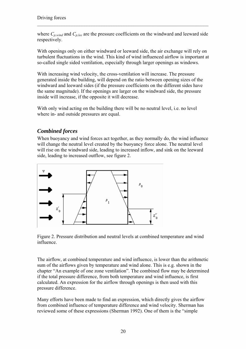
Combined forces When buoyancy and wind forces act together, as they normally do, the wind influence will change the neutral level created by the buoyancy force alone. The neutral level will rise on the windward side, leading to increased inflow, and sink on the leeward side, leading to increased outflow, see figure 2.

Figure 2. Pressure distribution and neutral levels at combined temperature and wind influence. The airflow, at combined temperature and wind influence, is lower than the arithmetic sum of the airflows given by temperature and wind alone. This is e.g. shown in the chapter “An example of one zone ventilation”. The combined flow may be determined if the total pressure difference, from both temperature and wind influence, is first calculated. An expression for the airflow through openings is then used with this pressure difference. Many efforts have been made to find an expression, which directly gives the airflow from combined influence of temperature difference and wind velocity. Sherman has reviewed some of these expressions (Sherman 1992). One of them is the “simple

20

Driving forces _____________________________________________________________________ quadrature” model, (Sherman 1980; Sherman and Grimsrud 1980).

Another expression is the “variable flow exponent” model,

22,

21,

2VVV qqq +=

nV

nV

nV qqq 1

2,1

1,1 +=

(Reardon 1989). In both these expressions, the indices 1 and 2 refer to buoyancy driven and wind driven airflow respectively. Lyberg investigated some other expressions and compared them to experimental data (Lyberg 1982). He found that a model of the type , best described experimental data.

γ)**( 2ubTaqV +∆=

21

Ventilation systems _____________________________________________________________________

Ventilation systems

Natural ventilation The expression “natural ventilation” may have different meanings. A building with “no” ventilation, i.e. no purposely-designed ventilation system, is a naturally ventilated building. But a building with carefully designed ventilation chimneys and supply openings, maybe even regulated, is also a natural ventilated building. Thus one has to be careful when using the expression and try to make a more specific description of the ventilation system. Characteristic for all naturally ventilated buildings is that natural forces, i.e. not mechanical, are used to create the air movements through the building. These natural forces are the buoyancy forces, due to density differences between inside and outside air, and wind forces, due to the dynamic energy in the wind. The natural forces may act by them self or in combination. In tropical countries, the natural ventilation may be depending on only wind forces, while buoyancy forces may be the most importing factor in northern countries. The natural forces create pressure differences across the building envelope, directed inwards on some surfaces and directed outwards on other. These pressure differences, make outside air infiltrate through cracks or purposely provided supply openings and exfiltrate trough cracks or ventilation chimneys. Depending upon the climatic conditions, and the construction of the building, air may flow in unintended directions, i.e. flow into the building through a ventilation chimney or leave the building through a supply opening. In the first case we get what is called a back draft, which deteriorates the function of the ventilation severely. One big advantage with natural ventilation is the absence of fans. This reduces both the energy cost for these and the sound level. The system also becomes very simple in its design. One big disadvantage is the natural fluctuation in airflow, with too low flows at high outside temperatures and calm weather and too high flows in winter and at windy weather. Another disadvantage is the risk for draught, since the supply air isn’t preheated; the difficulties to filter the supply of outside air, if it is of poor quality, and the difficulty too recover heat from the exhaust air. The latter depends on the very low pressure differences that are on hand in a naturally ventilated house. Since heat recovery also lowers the temperature in the ventilation chimney, the buoyancy driving force is decreased. Wind induced airflow thus becomes more important and has to be more utilized. There is however a need for assisting fans at low natural driving forces (Skåret, Blom et al. 1997). Schultz and Saxhof described a heat recovery equipment that in laboratory environment gave a heat recovery efficiency of 38 - 43% with corresponding temperature differences of 30 - 10 K (Schultz and Saxhof 1994). Shao et al showed that wire fin and plain fin type heat-pipe heat recovery units were superior to other investigated types (Shao, Riffat et al. 1998). Natural ventilation of today is something different than it used to be. This is because the supply, openings are known and may be chosen (Etheridge 2000). A condition for

22

Ventilation systems _____________________________________________________________________ this is of course that the building construction is tight and has few unintentional leakage openings.

Airflow in a ventilation chimney The ventilation chimney is the basic component of the PSV-ventilation system, passive stack ventilation. The chimney is a duct that functions as an extension of the building height, creating a higher air column. The higher the column of warm air, the larger the driving buoyancy force. A chimney also raises the neutral level, giving an under-pressure in a major part of the building. This reduces the risk of condensation in the building envelope. The gathering of exhaust flows, that is possible with the use of ventilation chimneys, is also a prerequisite for the possible use of heat recovery. The ventilation chimney creates a driving force that depends both on the temperature difference, between the warm air in the chimney and the cold air outside, and on the chimney height. In a simplified way, the airflow can be described as in figure 3. The created driving force, or driving pressure difference, depends on the whole height difference between the lowest air intake and the chimney top. This pressure difference is used to give airflow, not only through the chimney but also through external and internal openings. In normal calculations, the temperature in the chimney is assumed constant. In reality the air temperature is decreasing during its way up the chimney. This is of course decreasing the driving force and thus limiting the airflow. The temperature decrease depends upon the chimney insulation and the initial airflow through the chimney. 3 Figure 3. Simplified airflow through a building. In order to make an estimation of the errors connected with the assumed constant temperature, it is possible to model the ventilation chimney with the finite difference method. The temperature decrease, and its influence on the driving pressure and the airflow, may then be determined for the model.

23

Ventilation systems _____________________________________________________________________ However, some simplifications have to be made. One is to only study the driving pressure created in the chimney and the pressure loss in the chimney. Thus no consideration is taken to other created driving pressures and pressure losses in the building. Another simplification is that no consideration has been taken to asymmetry, i.e. different temperatures on different sides of the chimney, caused by for example solar radiation. The airflow through a 5 m ventilation duct with the inner diameter 100 mm is studied. The duct is assumed to be vertical, with its whole length located on the outside of the building, according to figure 3. Two cases are studied, assumed constant air temperature in the chimney (similar with completely insulated chimney) and steel chimney without insulation. The assumed inside temperature is 20 oC, corresponding to the inside density ρi = 1.205 kg/m3. The airflow has been calculated for –30, -10 and +10 oC outside temperature. Case 1 – completely insulated chimney If the temperature in the chimney is assumed to be constant, and the same as the inside temperature in the building, it is very easy to calculate the driving pressure as

( ) hgp iotot ⋅⋅−=∆ ρρ (6) With the assumed outside temperatures, the driving pressures are 12.16, 6.74 and 2.09 Pa respectively. The driving pressure gives cause to airflow through the chimney with the same pressure loss as the driving pressure. The pressure loss in a duct may be expressed as

25.0 udLfp iloss ⋅⋅⋅⋅=∆ ρ (7)

where f is the friction factor, L is the duct length, d is the duct inner diameter and u is the mean air velocity in the duct (Incropera and DeWitt 2002). Since ∆ploss must be equal to ∆ptot, we get an expression for the air velocity u

( )i

io

i

tot

Lfdhg

Lfdp

uρ

ρρρ ⋅⋅

⋅∆⋅⋅−⋅=

⋅⋅⋅∆⋅

=22

(8)

The Moody diagram gives an approximate value of the friction factor, f, as 0.0275. The driving pressures 12.16, 6.74 and 2.09 Pa thus give air velocities corresponding to the airflows 108.32, 80.67 and 44.90 m3/h respectively Case 2 – chimney without insulation The chimney, consisting of a 5 mm steel tube without insulation, is divided into 80 annular elements. The inner diameter of each element is 100 mm and the outer is 110 mm. The height of each element is 62.5 mm. The heat flow will be from the warmer air on the inside and in a radial direction towards the colder outside air.

24

Ventilation systems _____________________________________________________________________ Simultaneously there will be an axial heat flow through the chimney wall from the bottom to the top, see figure 4. We thus have a two-dimensional heat flow in the chimney wall. Figure 4. The heat flow through the chimney The temperature in the centre of each element is calculated. To this point, heat is received from the warm flowing air inside the chimney and from the somewhat warmer element below. Heat is transmitted to the colder air outside and to the somewhat colder element above. The temperature above the top element is the same as in the outside air while the temperature below the bottom element is the same as in the inside air. The UA-values (W/K), i.e. the inversed heat resistances in the different directions, have been calculated as follows. The UA-value between the centre of the element and the inside air is

=⋅ iAU

1

2

ln11

−

⎥⎥⎥⎥⎥

⎦

⎤

⎢⎢⎢⎢⎢

⎣

⎡

⋅

⎟⎟⎠

⎞⎜⎜⎝

⎛

+⋅⋅Π k

dd

dhli

m

ii (9)

where l is the element height, dm is the centre diameter, di is the inner diameter of the element, l is the length of one element, k is the conductivity of the material and hi is the convection heat transfer coefficient on the inside. The UA-value between the centre of the element and the outside air is

=⋅ oAU

1

2

ln11

−

⎥⎥⎥⎥⎥

⎦

⎤

⎢⎢⎢⎢⎢

⎣

⎡

⋅

⎟⎟⎠

⎞⎜⎜⎝

⎛

+⋅Π k

dd

dhlm

o

oo (10)

25

Ventilation systems _____________________________________________________________________ where do is the outer diameter of the element. The UA-value between the centre of the element and the upper border is the same as the UA-value between the centre and the lower border

( )l

ddkAUAU io

du ⋅−⋅Π⋅

=⋅=⋅2

22

(11) Simultaneously with the calculation of the temperatures in the wall, the air temperature in the chimney is calculated. The air column is also divided into 80 elements with assumed constant temperature in each element. To each air element heat is transported with the air flowing from the warmer element below. At the same time heat is transported via convection to the colder chimney wall. The following parameter values have been used for the calculation : The thermal conductivity for steel, ks, is 60 W/m, K. The convection heat transfer coefficient is 15 W/m2, K on the outside of the chimney, ho (Peterson 1980). The coefficient on the inside of the chimney is calculated as 6.319 . u 0.8. The latter expression is based on the Dittus-Boelter equation for turbulent flow in circular tubes, with used material properties for air.

3.054 PrRe023.0 ⋅⋅=Nu (12) (Incropera and DeWitt 2002) Although buoyancy forces cause the airflow through the chimney, we may use an expression for the heat exchange based on forced convection. This is because the airflow is caused by the total temperature difference between the air in the chimney and the air outside, and not explicit on the temperature differences at the inner chimney surface. Due to the continuity condition, the air velocity must be the same along every surface element, independent on the actual temperature difference at that element. The temperatures in the wall and in the air elements are determined by iterations. The air velocity u is also unknown from the beginning. The heat exchange between the air and the chimney wall depends on the velocity. At the same time, the velocity depends on the driving pressure in the chimney, which depends on the air temperatures, which depend on the heat rate. An air velocity has thus to be assumed before the iteration and then checked against the created driving pressure. The resulting temperatures in the wall and in the air will be according to figure 5. These results are obtained after some iteration with changing air velocity.

26

Ventilation systems _____________________________________________________________________

Figure 5. Temperatures in air and chimney wall. Outside temperature is –30 oC. 5 mm chimney without insulation. The driving pressure in the chimney can be derived from an expression similar to equation (6).

∑=

⋅⋅⎟⎟⎠

⎞⎜⎜⎝

⎛−⋅=∆

80

1 000

11i i

tot lgTT

Tp ρ (13)

where ρ0 is the air density at the temperature T0 = 0 oC. If the outside temperature is –30 oC, ∆ptot will be 3.65 Pa, i.e. clearly lower than the 12.16 Pa that a completely insulated chimney gives. Equation (8) now gives the air velocity 2.1 m/s corresponding to the airflow 59.36 m3/h. That is 45 % lower than the flow with a completely insulated chimney. The reduction in airflow depends on the outside temperature as well as the chimney wall thickness. The airflow through a 10 mm steel chimney, at –10 oC outside temperature, is approximately 1 % lower than through a 5 mm chimney at the same conditions. The explanation is that the heat resistance in the steel wall is very low compared to the resistances at the surfaces. The chimney with a thinner wall has a smaller outside area and is therefore favoured compared to a chimney with a thicker wall. Without insulation, the airflow through the chimney is much lower than is the case with a completely insulated chimney, see table 1. The reduction is largest when the airflow is strongest, i.e. at low outside temperatures.

27

Ventilation systems _____________________________________________________________________ Without insulation, the assumption of constant air temperature in the chimney thus gives large errors. With insulation, this error is decreased. The airflow with 100 mm insulation is approximately 10 % lower than with a completely insulated chimney. Even with this insulation, the error has a magnitude that can’t be neglected. Table 1. Calculated airflow through 5 mm steel chimney (m3/h), percentage of airflow through completely insulated chimney between brackets.

Airflow in m3/h (Compared to completely insulated chimney in %) Outside temperature No insulation 50 mm

insulation 100 mm insulation

Completely insulated

-30 oC 59.36 (54.8 %) 96.39 (89.0 %) 100.34 (92.6 %) 108.32 (100 %) -10 oC 45.81 (56.8 %) 71.36 (88.5 %) 74.36 (92.2 %) 80.67 (100 %) +10 oC 27.92 (62.2 %) 39.65 (88.3 %) 41.27 (91.9 %) 44.90 (100 %)

Mechanical ventilation Two types of mechanical ventilation are common; exhaust ventilation and supply-exhaust ventilation. The latter is also called balanced ventilation. In addition to these basic systems one may also use e.g. supply ventilation, intermittent ventilation and dynamic ventilation. The first mentioned types are, however, the most common and will be described here. Exhaust ventilation systems were the first to be used in Sweden and are today once again very popular. The system consists of an exhaust fan that, via exhaust ducts, extracts air from the “humid” rooms of the building. This decreases the pressures in these rooms. The extracted air must be replaced with supply air coming through openings in the outer and inner walls. If the building envelope is tight, the leakage openings in the outer walls are limited in size. Most of the supply air will then come from other rooms in the building. Since the “humid” rooms normally have a door to the hall, the air is taken from that. The pressure in the hall will therefore decrease and replacement air has to be taken from surrounding rooms. It’s easiest to draw air from rooms to which outside air may easily enter. These rooms are e.g. living room and bedrooms, which are equipped with special supply openings, or grilles. In this way, a desired air movement from “dry” to “humid” rooms is achieved. In the seventies, the exhaust ventilation was replaced by supply-exhaust ventilation in most new residential buildings. This was due to the difficulty to recover the heat energy in the exhaust air, together with the increasing interest in saving energy during this period. Since the second half of the eighties, thanks to the availability of exhaust air heat pumps, the use of exhaust ventilation has once again increased. The advantages of exhaust ventilation are the simplicity, with a minimum of ducts, the direct supply of outside air (if it is of good quality) and the stability of the system due to the created under-pressure. The low pressure in the building creates high pressure differences across the openings in the building shell. Pressures created by natural

28

Ventilation systems _____________________________________________________________________ forces are low compared to these, which means that changes in the outer climate has small influence on the airflow. A condition for this is that the exhaust system works with high pressure differences. Exhaust ventilation systems working with lower pressures may not be as stable. The drawbacks of exhaust ventilation are the risk for draught, which is connected to supply of unheated outside air, the difficulties to filter the supply of outside air, if it is of poor quality, and the low pressure in the building that may cause problems with noise and difficult opening of doors. A supply-exhaust ventilation system gives the best opportunities to control the air distribution and the air movements in the building. Preheated and filtered air (even cooled, humified or dehumified if desired) is supplied to desired rooms with a supply fan and a supply duct system. At the same time an exhaust fan with an exhaust duct system, removes air in the same way as with the exhaust system. With both supply and exhaust air in ducts, there are many possibilities to recover heat from the exhaust air. Both regenerative and recuperative methods are used. With the help of heat recovery batteries, heat may be recovered even if the ducts are located far away from each other. The advantage of the supply-exhaust system is the possibility to control the air movements, to heat and filter the supply air and to recover heat. The disadvantages are the high installing cost, due to increased duct length, and the instability of the system if the building isn’t tight enough. Since the system is balanced, with approximately the same airflows mechanically supplied and exhausted, no high pressure differences are created over the building shell. Natural forces may then influence the building in the same way as a naturally ventilated building. In order to keep the desired airflows in the building, the building shell has to be very airtight. Another disadvantage is the sound generation in both supply and exhaust grilles.

Hybrid ventilation Hybrid ventilation may be seen as an effort to combine the advantages of mechanical and natural systems (and hopefully avoid the disadvantages). Before hybrid ventilation was defined as a concept of its own, natural ventilation with mechanical aid has been used. At least in Sweden it has been common with intermittent use of exhaust fans from kitchen and bathroom/WC. Passive stack ventilation systems with added fan in the exhaust chimney and regulated supply vents came in the late 80’s. The outside temperature normally controls the fan and the supply vents. At low outside temperatures the system is purely a natural one. With higher outside temperatures, and low buoyancy force, the fan rotational speed increases. At low outside temperatures, the supply vents close to a minimum opening. This system is often called fan reinforced natural ventilation (Hecktor and Rämnér 1988). The system is also suitable for retrofitting of natural ventilation systems (Eriksson, Masimov et al. 1986). Hybrid ventilation as a concept was introduced in the late 90’s for office and school buildings. “Hybrid ventilation systems can be described as systems providing a

29

Ventilation systems _____________________________________________________________________ comfortable internal environment using both natural ventilation and mechanical systems, but using different features of the systems at different times of the day or season of the year. It is a ventilation system where mechanical and natural forces are combined in a two mode system” (Heiselberg 1999). Hybrid ventilation may also be seen as a low-pressure exhaust ventilation system, in which the fan is switched off at lower outside temperatures or higher wind velocities. Control of the system, and the switch between the two modes, may be more or less advanced. Temperatures, volume flows or CO2-concentrations in different rooms may control fans and ventilation openings. A control strategy for the shift between the modes is a key factor in hybrid ventilation and makes it different from other ventilation systems (Li 2001b).

30

Leakage through openings _____________________________________________________________________

Leakage through openings The openings in a building are of different types. One may differ between cracks, purposely made supply and exhaust openings and windows and doors. Cracks are unintended leakage ways in a buildings envelope. They often appear in joints between walls and floor or ceiling or around windows and doors. In many naturally ventilated buildings, airflow through the cracks is the only source to air exchange. In a building with purposely provided openings, however, one wants to minimize the number and size of the cracks. This is done by tightening around windows and doors and/or through the use of impermeable materials on the inside of the building shell. Pressurizing of the building is a method to estimate the influence of the cracks. This is normally made by the use of a fan, mounted in a door blade that replaces the ordinary door blade. The fan flow is controlled in such a way that the pressure in the building is either 50 Pa above or 50 Pa below the outside pressure. The airflow at that pressure is measured. This airflow at 50 Pa pressure difference may either be expressed as an air exchange, when the airflow in m3/h is divided by the building volume, or as airflow per m2 building shell area, when the surrounding area divides the airflow. In the Swedish Building Code (Boverkets byggregler, BBR, (BFS 2002:19)), the maximum accepted flow rate at 50 Pa pressure difference is 0.8 l/s and m2 surrounding area Expressions for the calculation of airflow through a leakage opening are, as all airflows, based on the Navier-Stokes equation. This is a non-linear partial differential

equation in , the velocity vector. →

u

→→→→→

+∇+∇−=∇⋅+∂∂ Fupuu

tu

ρν

ρ11 2 (14)

→

F is known as the body force term and represents the contribution of forces that act on the volume of a fluid particle, such as gravity (Tritton 1988). The left hand of the equation is the net change of momentum of a fluid particle, with time and in different directions. The right side is the sum of the forces acting on the fluid particle, the pressure force, the viscous force and the body force. If the flow is assumed to be a steady incompressible flow, and the Reynolds number is so high that the viscous term may be neglected compared to the inertia force, we get Euler’s equation of inviscid motion. The body force term is here omitted (Tritton 1988).

puu −∇=∇⋅→→

ρ (15)

31

Leakage through openings _____________________________________________________________________ If the component of Euler’s equation in the streamline direction is integrated, we will get the well-known Bernoulli’s equation

=+⋅⋅ pu 25.0 ρ constant (16) where u is the velocity component in the streamline direction (Tritton 1988). This is Bernoulli’s equation in its pressure form, in which all terms have the dimension Pa. It means that the sum of dynamic and static pressure is constant along a streamline. If this equation is used for both sides of an orifice opening, assuming zero velocity on the high-pressure side, we get the theoretical velocity out of the opening.

( )ρρ

ρ pppupup ∆⋅

=−

=⇒+⋅⋅=22

5.0 2122

221 (17)

This means that the volume flow rate through the orifice will be

ρpAqV

∆⋅⋅=

2 (18)

where A is the cross section area of the opening. Equation (18) gives the volume flow rate through an orifice, with a pressure difference ∆p across it, if there are no losses. In reality the velocity u2 will be less than the calculated, due to friction losses. At the same time the real useful cross section area will be smaller than A, due to the contraction of the jet out of the opening. The mass flow rate will thus be

ρρ pACm D

∆⋅⋅⋅⋅=

• 2 (19)

where CD is the so-called discharge coefficient for the opening. It is defined as the ratio between the real and the theoretical flow rate. For a sharp-edged opening this coefficient will be close to 0.6 while it is typical 0.65-0.70 for an opening in the building envelope. Bernoulli’s equation (eq 16) is not possible to use for the fully developed laminar flow in a pipe, since it doesn’t take viscosity into consideration (Herrlin 1986). For this purpose, the following equation for so-called Hagen-Poiseuille flow is used.

µ⋅⋅⋅∆

=Ldpuav 32

2

(20)

where uav is the average air velocity in the pipe and L is the length of the pipe. The equation may be rewritten to give the pressure drop in the pipe, ∆p.

32

Leakage through openings _____________________________________________________________________

226432 22

22avavav u

dLfu

duL

duL

p⋅

⋅⋅

=⋅

⋅⋅

⋅⋅=

⋅⋅⋅=∆

ρρνµ (21)

where f is the friction factor that is 64/Re for laminar flow (Incropera and DeWitt 2002). According to the first part of equation (21), the pressure drop is directly proportional to the velocity at laminar flow, and thus also to the flow rate. At fully developed turbulent flow in rough pipes, Darcy’s formula is

2

2avu

dLfp

⋅⋅

⋅=∆

ρ (22)

(Herrlin 1986) At turbulent flow, the friction factor f is almost independent of Re at higher Re-numbers. At these Re-numbers it depends on the roughness ε and may be found in the so-called Moody's diagram. The pressure drop at fully developed turbulent flow in pipes is proportional to the square of the velocity, and thus the square of the flow rate, according to equation (22). Depending on the type of flow, the volume flow rate through a pipe is thus either directly proportional to the pressure difference or proportional to the square of it.

1pantconstqV ∆⋅= (at laminar flow) or (at turbulent flow) 5.0pantconstqV ∆⋅= Based on these expressions for volume flow in a pipe, the mass flow through a leakage opening may be expressed with the so-called power law (Herrlin 1992).

npCm ∆⋅=•

(23) where C is the flow coefficient and n is the flow exponent that is between 0.5 and 1. This flow coefficient is determined at a specific temperature and pressure. If the actual state of the air is different a correction factor is used. Many suggestions of practical values of the exponent n exist in the literature. A common opinion is that a building, with its different types of leakage openings, has a mixture of leakages with both laminar and turbulent airflow. The pressure drop shall then be proportional to the airflow raised to 1.5, i.e. the exponent n is 0.67. This is also the approximate value of n one gets as a result from test pressurizing of buildings. According to Peterson either laminar or turbulent airflow exists in fully developed form in the short leakage ways that exist in a building. He has shown that the exponent n has a value between 0.67 and 0.77 when the airflow is not fully developed (Peterson 1982).

33

Leakage through openings _____________________________________________________________________ 2/3 is perhaps the most often used value on the exponent n at adaptation of measured air leakage to wind and temperature data. Both 0.5 and 1.0 are however used and according to Lyberg, the value 0.5 will give a better adaptation than both 0.6 and 0.7 (Lyberg 1982). The area of the leakage openings is often determined at pressure differences much larger than the practical differences, e.g. through pressurization. It’s therefore normal praxis to convert the flow rate qV, tot at a specific pressure difference ∆p to an equivalent, or effective, leakage area, Aeq. This is the area of a sharp-edged orifice opening in a thin wall, which would give the same flow rate at the specific pressure difference (Kronvall 1983; Etheridge and Sandberg 1996).

ρpC

qA

D

totVeq ∆⋅

⋅=

2, (24)

where Aeff is the equivalent, leakage area. Herrlin defines the effective leakage area, ELA, as the area that a sharp-edged orifice opening should have to give the same flow rate, at 4 Pa pressure difference, when the discharge coefficient CD = 1 (Herrlin 1992).

424 ⋅⋅=

ρPaqELA (25)

The flow at 4 Pa pressure difference, q4 Pa, is often determined through pressurization at a higher pressure difference, e.g.50 Pa. That means that the value of q4 Pa depends on the assumed flow exponent n since

( ) Pan

Pa qq 504 504 ⋅= (26) When the effective leakage area ELA is used, the mass flow rate is calculated as

nn pELAm ∆⋅

⋅⋅⋅=

•

424 ρ

(27)

(EQUA Simulation 2001)

34

Airflow modelling _____________________________________________________________________

Airflow modelling There are different ways of modelling the airflows in a building. One may separate two sets of fluid dynamics equations that are often used; the Bernoulli equation and the Navier-Stokes equations. The Bernoulli equation is mainly used for simple analytical and empirical methods and multi zone methods, while the Navier-Stokes equations are used for computational fluid dynamics methods, CFD (Li 2001a)..

Analytical methods Simple analytical and empirical methods are generally applied to simple geometry buildings, e.g. single-sided ventilation and one-zone ventilation. These kinds of methods are important as tools for e.g. the designer of a building. The analytical method gives an exact mathematical solution to the equations concerned. If the building has an open interior it may be treated as one zone. In other cases one may want to study a room that isn’t connected to the rest of the building, i.e. single-sided ventilation. Analytical methods have their limitations when it comes to both number

zones and number of openings. of A number of analytical and experimental studies have been performed. Dascalaki et al have e.g. compared measurements of the ventilation in a single-sided room with the results of network models (Dascalaki, Santamouris et al. 1995). Linden et al investigated natural ventilation in a one-zone building with openings at two levels. Airflow and thermal stratification was determined for different heat sources (Linden, Lane-Serff et al. 1990). The results have been confirmed by e.g. Chen et al using a fine-bubble modelling technique (Chen and Li 2002). Analytical studies of the airflow and the stratification level in one-zone buildings have also been performed by e.g. Cooper and Hunt (Cooper and Hunt 1999), Li (Li 2000) and Chen and Li (Chen and Li 2002).

An example of one-zone ventilation The following text is based on work accomplished by the author during the years 1983–84. The original calculations were performed with an ordinary calculator. The figures are however new plots. In this text, air leakage is defined as all the airflow that passes through the buildings envelope. This airflow may either be intended or unintended. When natural ventilation is used, the air leakage constitutes the whole ventilation flow. Air leakage up to a certain level is then necessary. Even with mechanical exhaust ventilation, an air leakage corresponding to the required ventilation flow is necessary. Air leakage above this level leads to increased heat losses but may be positive for the indoor climate.

35

Airflow modelling _____________________________________________________________________ Only when mechanical supply-exhaust ventilation is used, all air leakage is unwanted. In this case the ventilation system provides the whole required ventilation flow and air leakage only means unnecessary ventilation and increased heat losses. Three different driving forces give the airflow in a building. These forces may act one at a time or in combination. The three forces are a) pressure differences across the building envelope created by temperature

differences between in- and outside. b) pressure differences across the building envelope created by positive or negative

wind pressures on the building. c) pressure differences across the building envelope created by mechanical

ventilation system, either exhaust ventilation or unbalanced supply-exhaust. For each driving force the air leakage qV may be expressed as

bV xaq ⋅= (28)

where x is the temperature difference with driving force a), the wind speed with driving force b) or unbalance in ventilation airflow with driving force c). The constants a and b may be determined for each specific building through measurements. A precondition for this is, however, that only one driving force acts at a time. If two or three driving forces act simultaneously, it’s more difficult to determine the constants a and b through measurements. A mathematical model of a building is assumed, consisting of one cell, i.e. without inner walls, and with a flat roof. When wind occurs, it is assumed to attack at right angle. One of the facades is then the windward side while the others are leeward sides. The wind pressure at each facade is assumed constant, both over the surface and with time. On the windward side, the over-pressure is assumed 70 % of the dynamic pressure in the free wind, i.e. the pressure coefficient Cp1 is 0.7. At the roof and on the leeward sides, the under-pressure is assumed to be 80 % of the over pressure on the windward side, i.e. the pressure coefficient Cp2 is -0.56. The building’s leakage openings are assumed evenly distributed over walls and roof. The leakage ratios kw and kr have been used as measures of the leakage opening sizes, per m2 of wall or roof area,. The air leakage has been calculated for this model at three different conditions: 1) Influence of temperature difference alone 2) Influence of wind alone 3) Combined influence of temperature and wind

36

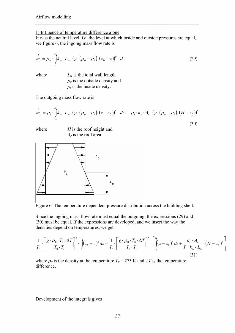
Airflow modelling _____________________________________________________________________ 1) Influence of temperature difference alone If z0 is the neutral level, i.e. the level at which inside and outside pressures are equal, see figure 6, the ingoing mass flow rate is

( ) ( )(∫ −⋅−⋅⋅⋅⋅=• 0

00

zn

iowwoi dzzzgLkm ρρρ )

)

(29) where Lw is the total wall length ρo is the outside density and ρi is the inside density. The outgoing mass flow rate is

( ) ( )( ) ( ) (( )niorri

H

z

niowwio zHgAkdzzzgLkm 00

0

−⋅−⋅⋅⋅⋅+−⋅−⋅⋅⋅⋅= ∫•

ρρρρρρ

(30) where H is the roof height and Ar is the roof area

Figure 6. The temperature dependent pressure distribution across the building shell. Since the ingoing mass flow rate must equal the outgoing, the expressions (29) and (30) must be equal. If the expressions are developed, and we insert the way the densities depend on temperatures, we get

( ) ( ) ( )∫ ∫⎥⎥⎦

⎤

⎢⎢⎣

⎡−⋅

⋅⋅⋅

+−⋅⎥⎦

⎤⎢⎣

⎡⋅

∆⋅⋅⋅⋅=−⋅⎥

⎦

⎤⎢⎣

⎡⋅

∆⋅⋅⋅⋅

0

0000

000

0

00 11 z H

z

n

wwi

rrnn

ioi

nn

io

zHLkT

AkdzzzTT

TTgT

dzzzTT

TTgT

ρρ

(31) where ρ0 is the density at the temperature T0 = 273 K and ∆T is the temperature difference. Development of the integrals gives

37

Airflow modelling _____________________________________________________________________

( )( )

( ) ( ) ⇒−⋅⋅⋅

⋅+

+⋅−

=+⋅

++n

wwi

rr

i

n

o

n

zHLkT

AknTzH

nTz

0

10

10

11

( )( ) ( 10

0

10 +⋅⋅⋅=−⋅−−

+

nHsTT

zHTT

zHz

i

o

i

on

n

) (32)

where s is the leakiness ratio, defined as s = wrwr AAkk ⋅ and Aw is the total wall area = H . Lw If the roof is totally tight, i.e. s = 0, the neutral level z0 may easily be calculated as

110

1+

⎟⎠⎞⎜

⎝⎛+

= n

o

iT

THz (33)

If kr > 0, the neutral level z0 has to be calculated through iteration. When the neutral

level is determined, it’s possible to calculate the leakage mass flow rate, , that is equal to in- and outgoing mass flow, with the help of equation (29) or (30).

•

Lm

2) Influence of wind alone With influence only of wind, air will flow into the building through the facades on which the wind give an over pressure. Simultaneously, air will flow out through the leeward sides, i.e. facades where the wind generates an under pressure. This is called cross ventilation. In the used building model the roof is assumed to be flat. This means that also the roof will have an under pressure. This is assumed to be the same as the leeward walls. Air will thus flow out through the roof if it is not tight. If the windward walls, with positive wind pressure, have the total area Awind, the mass flow rate into the building will be

n

io

pwindwoi pu

CAkm ⎟⎟⎠

⎞⎜⎜⎝

⎛−

⋅⋅⋅⋅⋅=

•

2

2

1ρ

ρ (34)

where u is the wind velocity and pi is the pressure inside the building at floor level. The mass flow rate out of the building is

n

io

prri

n

io

pleewio pu

CAkpu

CAkm ⎟⎟⎠

⎞⎜⎜⎝

⎛+

⋅⋅⋅⋅⋅+⎟⎟

⎠

⎞⎜⎜⎝

⎛+

⋅⋅⋅⋅⋅=

•

22

2

2

2

2ρ

ρρ

ρ (35)

where Alee is the total area of the leeward walls.

38

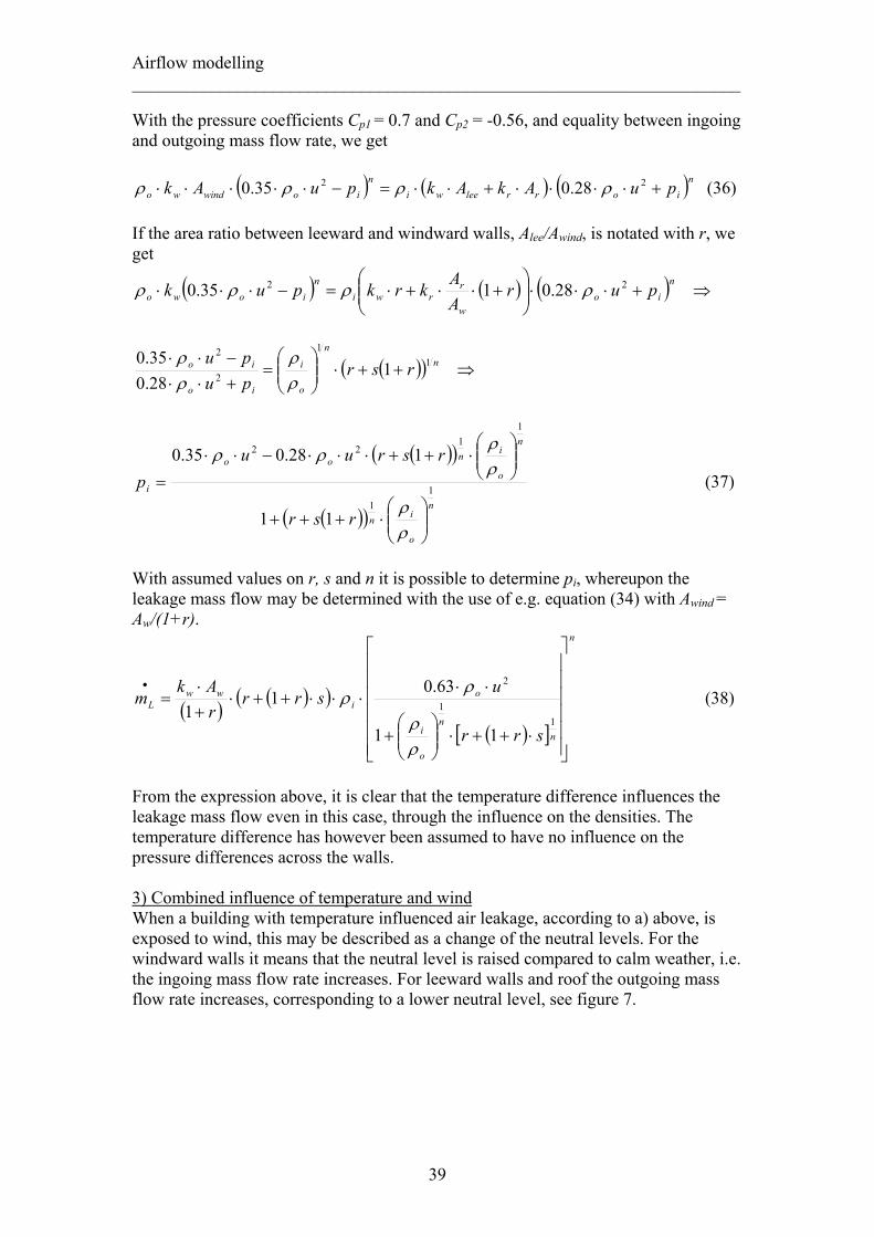
Airflow modelling _____________________________________________________________________ With the pressure coefficients Cp1 = 0.7 and Cp2 = -0.56, and equality between ingoing and outgoing mass flow rate, we get

( ) ( ) ( )niorrleewi

niowindwo puAkAkpuAk +⋅⋅⋅⋅+⋅⋅=−⋅⋅⋅⋅⋅ 22 28.035.0 ρρρρ (36)

If the area ratio between leeward and windward walls, Alee/Awind, is notated with r, we get

( ) ( ) ( ) ⇒+⋅⋅⋅⎟⎟⎠

⎞⎜⎜⎝

⎛+⋅⋅+⋅=−⋅⋅⋅

nio

w

rrwi

niowo pur

AAkrkpuk 22 28.0135.0 ρρρρ

( )( ) ⇒++⋅⎟⎟⎠

⎞⎜⎜⎝

⎛=

+⋅⋅−⋅⋅ n

n

o

i

io

io rsrpupu 1

1

2

2

128.035.0

ρρ

ρρ

( )( )

( )( )n

o

in

n

o

inoo

i

rsr

rsruup 1

1

11

22

11

128.035.0

⎟⎟⎠

⎞⎜⎜⎝

⎛⋅+++

⎟⎟⎠

⎞⎜⎜⎝

⎛⋅++⋅⋅⋅−⋅⋅

=

ρρ

ρρ

ρρ (37)

With assumed values on r, s and n it is possible to determine pi, whereupon the leakage mass flow may be determined with the use of e.g. equation (34) with Awind = Aw/(1+r).

( ) ( )( )

( )[ ]

n

nn

o

i

oi

wwL

srr

usrr

rAk

m

⎥⎥⎥⎥⎥⎥

⎦

⎤

⎢⎢⎢⎢⎢⎢

⎣

⎡

⋅++⋅⎟⎟⎠

⎞⎜⎜⎝

⎛+

⋅⋅⋅⋅⋅++⋅

+⋅

=•

11

2

11

63.01

1

ρρ

ρρ (38)

From the expression above, it is clear that the temperature difference influences the leakage mass flow even in this case, through the influence on the densities. The temperature difference has however been assumed to have no influence on the pressure differences across the walls. 3) Combined influence of temperature and wind When a building with temperature influenced air leakage, according to a) above, is exposed to wind, this may be described as a change of the neutral levels. For the windward walls it means that the neutral level is raised compared to calm weather, i.e. the ingoing mass flow rate increases. For leeward walls and roof the outgoing mass flow rate increases, corresponding to a lower neutral level, see figure 7.

39

Airflow modelling _____________________________________________________________________

Figure 7. The pressure distribution across a building with combined temperature and wind influence. If the neutral level is z0´ for the windward walls and z0´´ for the leeward walls and roof, according to figure 9, the ingoing mass flow rate is

( )( ) ( )( ) ⇒−⋅∆⋅⋅⋅+−⋅∆⋅⋅= ∫ ∫•

'0

''0

0 0

''0

'0

z zn

leewo

n

windwoi dzzzgLkdzzzgLkm ρρρρ

( ) ( ) ( )( ) ( )[ ]1''

01'

011++•

⋅++⋅+

⋅⋅∆⋅⋅=

nnwwnoi zrz

nrHAk

gm ρρ (39)

The outgoing mass flow rate is

( )( ) (( ) +−⋅∆⋅⋅⋅+−⋅∆⋅⋅⋅= ∫ ∫• H

z

H

z

n

leewi

n

windwio dzzzgLkdzzzgLkm'

0''

0

''0

'0 ρρρρ )

)

( )( ⇒−⋅∆⋅⋅⋅⋅+n

rri zHgAk ''0ρρ

( ) ( )( )

( ) ( )( )( )

( ) ( ) ( )⎟⎟

⎠

⎞

⎜⎜

⎝

⎛−+

+⋅+−⋅

++⋅+

−⋅⋅⋅∆⋅⋅=

++• n

nn

wwn

io zHsnrH

zHrnrH

zHAkgm ''

0

1''0

1'0

1111ρρ (40)

Lwind and Llee are the lengths of the windward and leeward sides respectively. The ratio Llee/Lwind is equal to the area ratio r = Alee/Awind . Since ingoing and outgoing mass flow must be equal, we get

( ) ( ) ( )( ) ( )( ) ( ) ( ) ([ ]nnn

i

onn zHHnrszHrzHTT

zrz ''0

1''0

1'0

1''0

1'0 11 −⋅+⋅++−+−=⋅+

++++ ) (41)

To calculate the new neutral levels, z0´ and z0´´, we need one more equation. We get it by studying how the neutral levels change on windward and leeward walls. On the windward walls there is an increase of the pressure directed inwards that is corresponding to an increase of the neutral level.

40

Airflow modelling _____________________________________________________________________

ρρ

ρ

ρρ

∆⋅−⋅⋅

+=⇒⋅∆⋅

−⋅

⋅+⋅∆⋅=

gpu

zzzg

pu

Czg

zz io

io

p 2

0'0

0

2

10

0

'0 35.02 (42)

where z0 is the neutral level with temperature influence alone. In a similar way we get a decrease of the pressure directed inwards on leeward walls and roof and a corresponding decrease of the neutral level.

ρρ

ρ

ρρ

∆⋅+⋅⋅

−=⇒⋅∆⋅

−⋅

⋅+⋅∆⋅=

gpu

zzzg

pu

Czg

zz io

io

p 2

0''

00

2

20

0

''0 28.02 (43)

These last two equations together, give a relation between z0´ and z0´´.

ρρ∆⋅

⋅⋅+=

gu

zz o2

''0

'0

63.0 (44)

The equations (41) and (44) now constitute an equation system with two unknown, the neutral levels z0´ and z0´´. When these unknown neutral levels are solved, it is

possible to determine the leakage value , equal to , with equation (39). •

Lm•

imEquations (39) and (41) are, however, valid only as long as the neutral levels, z0´ and z0´´, lie between the buildings bottom and top, i.e. 0 < z0´ (z0´´) < H. As the wind velocity increases, the neutral levels eventually end up outside these boundaries. Which level that first leaves the boundaries depends, among other things, on the distribution of leakage openings between roof and walls, and on the value of the leakiness ratio s. As one of the neutral levels moves outside the boundaries, equations (39) and (41) have to be rewritten. With only temperature and wind influence, i.e. no mechanical ventilation, the following airflow patterns, and equations, are possible. Case 1 0 < z0´ < H 0 < z0´´ < H

( ) ( ) ( )( ) ( )[ ]1''

01'

011++•

⋅++⋅+

⋅⋅∆⋅⋅=

nnwwnoi zrz

nrHAk

gm ρρ (39)

( ) ( ) ( )( ) ( )( ) ( ) ( ) ( )[ ]nnn

i

onn zHHnrszHrzHTT

zrz ''0

1''0

1'0

1''0

1'0 11 −⋅+⋅++−+−=⋅+

++++ (41)

41

Airflow modelling _____________________________________________________________________ Case 2 z0´ > H 0 < z0´´ < H

( ) ( ) ( )( ) ( ) ( )( )[ ]1'

01''

01'

011+++••

−−⋅++⋅+

⋅⋅∆⋅⋅==

nnnwwnoi Hzzrz

nrHAk

gmm L ρρ (45)

( ) ( ) ( )( ) ( )( ) ( ) ( ) ( )[ ]nn

i

onnn zHHnrszHrTT

Hzzrz ''0

1''0

1'0

1''0

1'0 11 −⋅+⋅++−=−−⋅+

++++ (46)

Case 3 0 < z0´ < H z0´´ < 0

( ) ( ) ( )( )1'

011+••

⋅+⋅+

⋅⋅∆⋅⋅==

nwwnoi z

nrHAk

gmm L ρρ (47)

( ) ( )( ) ( )( ) ( )( ) ( ) ( ) ([ ]nnnn

i

on zHHnrszrzHrzHTT

z ''0

1''0

1''0

1'0

1'0 11 −⋅+⋅++−−−+−=

++++ ) (48)

Case 4 z0´ > H z0´´ < 0

( ) ( ) ( )( ) ( )( )[ ]1'

01'

011++••

−−+⋅+

⋅⋅∆⋅⋅==

nnwwnoi Hzz

nrHAk

gmm L ρρ (49)

( ) ( )( ) ( )( ) ( )( ) ( ) ( ) ([ ]nnn

i

onn zHHnrszrzHrTT

Hzz ''0

1''0

1''0

1'0

1'0 11 −⋅+⋅++−−−=−−

++++ ) (50)

When the air leakage is calculated, it is thus necessary to know which of the mentioned airflow cases that is by the hand at the actual temperature difference and wind velocity. Iterations are used to determine the neutral levels so that in and

42

Airflow modelling _____________________________________________________________________ outgoing mass flow rates are equal. The right equations for airflow are continuously chosen, based on the calculated neutral levels. Results Figure 8 shows the air leakage when only the temperature difference is influencing the airflow, i.e. at calm weather. The air leakage volume flow is shown as a function of the temperature difference at different leakiness ratios s for the building. The value of kw . Aw for the building is assumed to be 0.006. The building height is 2.5 m and the inside temperature is 20 oC. The calculations have been performed for different values of the flow exponent n, though only the case with n = 0.7 is showed in the figure. The air leakage is shown as volume airflow rates at 20 oC.

Figure 8. The air leakage with different values on the leakiness ratio s. Temperature influence alone. n = 0.7. As the temperature difference increases from zero to approximately 2 K, the air leakage increases rapidly. From there on it increases slower and from 10 – 15 K the increase is almost linear. The leakiness ratio s is a measure of the leakage opening size of the roof compared to that of the walls. It’s clear from the figure that the air leakage is approximately twice as large, if the leakiness ratio s = 0.6, compared to a completely tight roof, s = 0. The leakiness ratio s is 0.6 if, e.g. kr/kw = 0.5 and Ar/Aw = 1.2. This means that the roof is half as leaky as the walls. The ratio between roof and wall area, Ar/Aw, = 1.2 corresponds for example to a quadratic detached building, r = 3, with the side 12 m and the height 2.5 m. It may also correspond to a middle part of a terraced house, r = 1, with the width 6 m and the depth 6 m. As shown in the figure, the air leakage increases with increasing temperature difference, i.e. lower outside temperature. It also increases with increased s, i.e. with

43

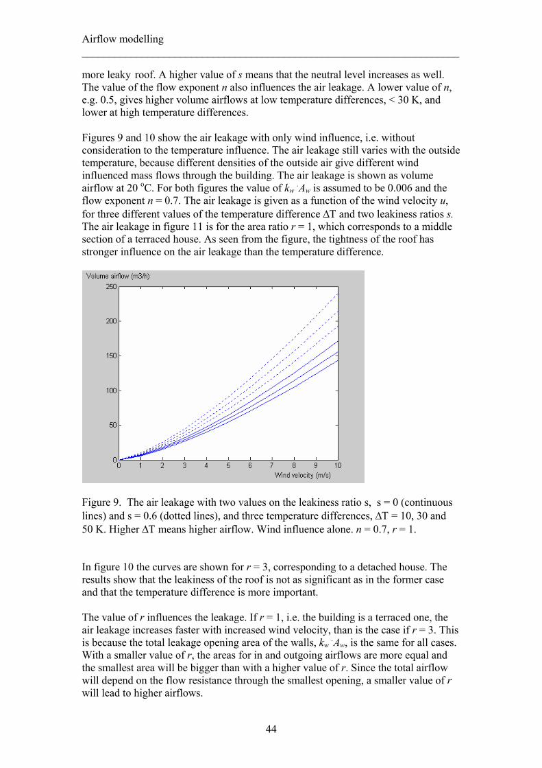
Airflow modelling _____________________________________________________________________ more leaky roof. A higher value of s means that the neutral level increases as well. The value of the flow exponent n also influences the air leakage. A lower value of n, e.g. 0.5, gives higher volume airflows at low temperature differences, < 30 K, and lower at high temperature differences. Figures 9 and 10 show the air leakage with only wind influence, i.e. without consideration to the temperature influence. The air leakage still varies with the outside temperature, because different densities of the outside air give different wind influenced mass flows through the building. The air leakage is shown as volume airflow at 20 oC. For both figures the value of kw .Aw is assumed to be 0.006 and the flow exponent n = 0.7. The air leakage is given as a function of the wind velocity u, for three different values of the temperature difference ∆Τ and two leakiness ratios s. The air leakage in figure 11 is for the area ratio r = 1, which corresponds to a middle section of a terraced house. As seen from the figure, the tightness of the roof has stronger influence on the air leakage than the temperature difference.

Figure 9. The air leakage with two values on the leakiness ratio s, s = 0 (continuous lines) and s = 0.6 (dotted lines), and three temperature differences, ∆Τ = 10, 30 and 50 K. Higher ∆Τ means higher airflow. Wind influence alone. n = 0.7, r = 1. In figure 10 the curves are shown for r = 3, corresponding to a detached house. The results show that the leakiness of the roof is not as significant as in the former case and that the temperature difference is more important. The value of r influences the leakage. If r = 1, i.e. the building is a terraced one, the air leakage increases faster with increased wind velocity, than is the case if r = 3. This is because the total leakage opening area of the walls, kw .Aw, is the same for all cases. With a smaller value of r, the areas for in and outgoing airflows are more equal and the smallest area will be bigger than with a higher value of r. Since the total airflow will depend on the flow resistance through the smallest opening, a smaller value of r will lead to higher airflows.

44

Airflow modelling _____________________________________________________________________

Figure 10. The air leakage with two values on the leakiness ratio s, s = 0 (continuous lines) and s = 0.6 (dotted lines), and three temperature differences, ∆Τ = 10, 30 and 50 K. Higher ∆Τ means higher airflow. Wind influence alone. n = 0.7, r = 3. Figure 11 and 12 show the air leakage at combined temperature and wind influence. The air leakage is given as a function of the wind velocity u at three different temperature differences ∆Τ and at two different area ratios r.

Figure 11. The air leakage with two values on the leakiness ratio s, s = 0 (continuous lines) and s = 0.6 (dotted lines), and three temperature differences, ∆Τ = 10, 30 and 50 K. Higher ∆Τ means higher airflow. Combined temperature and wind influence. n = 0.7, r = 1.

45

Airflow modelling _____________________________________________________________________ With the tight roof, continuous lines in figure 11, a higher temperature difference gives higher air leakage at low and high wind velocities. There is however a velocity interval during which the temperature difference has small affect

Figure 12. The air leakage with two values on the leakiness ratio s, s = 0 (continuous lines) and s = 0.6 (dotted lines), and three temperature differences, ∆Τ = 10, 30 and 50 K. Higher ∆Τ means higher airflow. Combined temperature and wind influence. n = 0.7, r = 3. Up to a certain wind velocity, the air leakage is more or less constant at a given temperature difference. It thereafter increases quickly with the wind velocity. At low wind velocities, the air leakage increases with increasing temperature difference. If the roof is tight, s = 0, the temperature influence on the air leakage first decreases, with increased wind velocity, and thereafter increases again. At higher wind velocities the temperature influence isn’t due to the buoyancy forces, but to the temperature influence on the density of the inflowing air It is also possible to see that the transition to a steeper slope takes place at higher wind velocities, the higher the temperature difference is. This is most obvious with tight roof, i.e. as s = 0. A high temperature difference, with its high temperature dependent air leakage, helps to hinder the pure wind depending air leakage to take control. With increasing wind velocity, there will be a transition in the airflow pattern, from case 1, buoyancy depending, to case 4, cross flow. This transition normally goes via one of the cases 2 or 3. With a terraced building, r = 1, case 3 follows after case 1 if the roof is tight. If the roof is quite leaky, s = 0.6 or if the building is detached, r = 3, there is first a transition to case 2. This is the case if the flow exponent n = 0.70. For other values of n the transitions may be different.

46

Airflow modelling _____________________________________________________________________ Table 2 shows the transitions, and the approximate wind velocities at which they appear, with the flow exponent n = 0.7 and for two area ratios, r = 1 and r = 3, two leakiness ratios, s = 0 and s = 0.6 and three temperature differences, ∆Τ = 50, 30 and 10 K. Table 2. Transitions between different flow patterns. n = 0.70. r s ∆Τ Transition Velocity Transition Velocity 1 0 50 1 - 3 2.46 3 - 4 2.74 30 1 - 3 1.94 3 - 4 2.07 10 1 - 3 1.15 3 - 4 1.16 0.6 50 1 - 2 1.83 2 - 4 3.88 30 1 - 2 1.38 2 - 4 3.14 10 1 - 2 0.77 2 - 4 1.90 3 0 50 1 - 2 2.17 2 - 4 3.85 30 1 - 2 1.66 2 - 4 3.12 10 1 - 2 0.95 2 - 4 1.88 0.6 50 1 - 2 1.62 2 - 4 6.60 30 1 - 2 1.23 2 - 4 5.32 10 1 - 2 0.69 2 - 4 3.23 These transitions explain the form of the curves in figures 11 and 12. It is first after the transition to case 4, cross flow ventilation, that the wind influenced ventilation dominates. Before that transition, the buoyancy driven ventilation has a larger importance. Which transition that first takes place depends on the ratio between the opening areas for in and outgoing airflow. With a low value on this ratio, the pressure difference has to be increased faster on the windward side. This is the case e.g. when r = 3 and the roof is leaky. The first transition is then to case 2. First after further wind increase the next transition to case 4 occurs. If the value is higher (closer to unity), which is the case when r = 1 and the roof is tight, the pressure difference has to increase faster on the leeward sides. The first transition is then to case 3. This transition is normally quickly followed by a transition to case 4. In figure 13, the curves for air leakage depending on temperature influence alone, wind influence alone and the algebraic sum of these curves are plotted in the same diagram. The combined air leakage is also plotted in the diagram. One finds that the combined air leakage is always lower than the algebraic sum. One also finds that the curve for combined leakage lies in an area, bounded by the three other curves. At low wind velocities, it lies close to the curve for temperature influence alone. At high velocities, it lies close to the curve for wind influence alone and it’s clear how the wind forces totally determine the air leakage at this wind velocities. The diagram is valid for the flow exponent n = 0.7, the area ratio r = 3, the temperature difference ∆Τ = 243 K and the leakiness ratio s = 0.6. Figure 14 shows

47

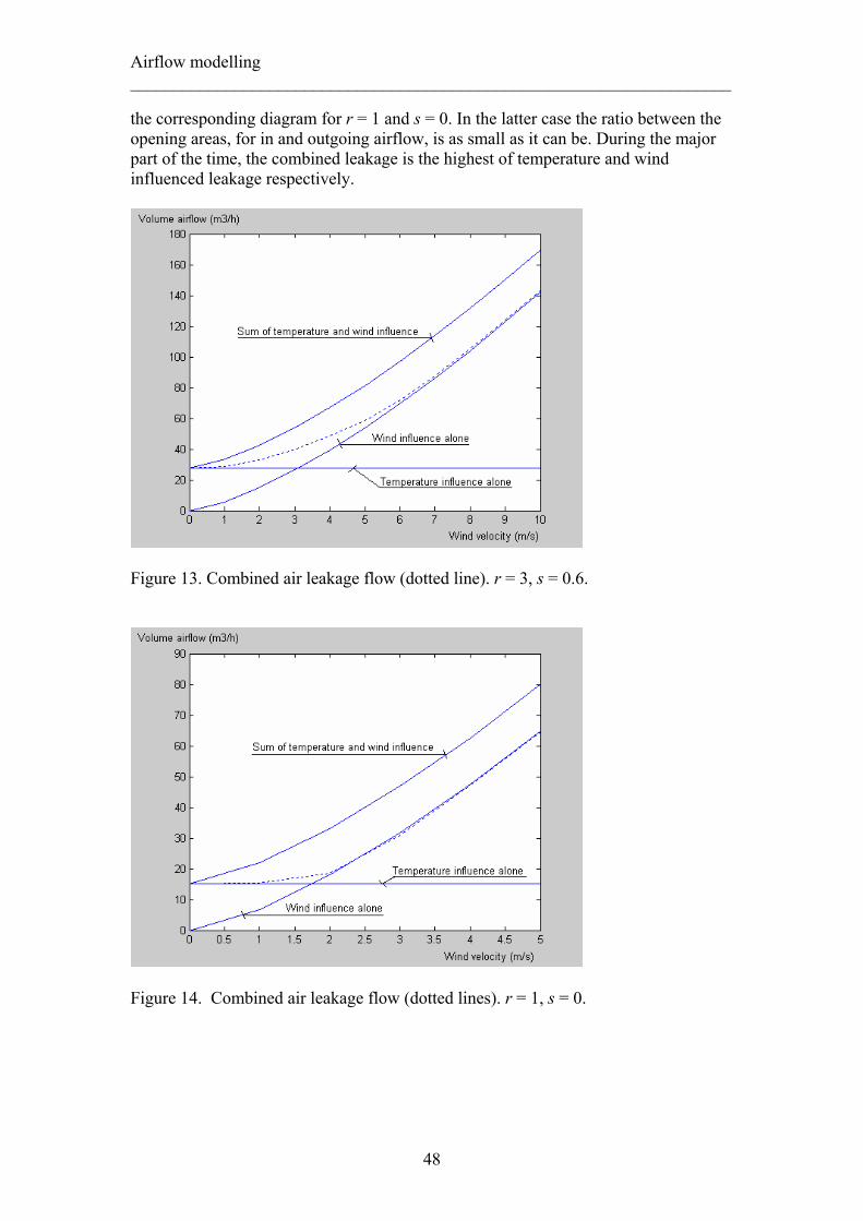
Airflow modelling _____________________________________________________________________ the corresponding diagram for r = 1 and s = 0. In the latter case the ratio between the opening areas, for in and outgoing airflow, is as small as it can be. During the major part of the time, the combined leakage is the highest of temperature and wind influenced leakage respectively.

Figure 13. Combined air leakage flow (dotted line). r = 3, s = 0.6.

Figure 14. Combined air leakage flow (dotted lines). r = 1, s = 0.

48

Airflow modelling _____________________________________________________________________ Multi zone models With the multi zone method, the building is divided into a number of zones, normally one zone per room. In each zone one may have uniform temperature or a temperature gradient. The temperature may be set as a parameter in the program or calculated simultaneously with the airflows. The latter requires that the airflow program be coupled to a thermal program. In each zone the pressure is assumed to have a hydrostatic variation (Axley, Wurtz et al. 2002). In this assumption lies an assumption that the air velocity in the zone is zero and that there is no pressure gradient in a horizontal level. Of course this is a contradiction of the task for the multi zone program – to calculate airflows. With assumed internal pressures at floor level in each zone, the pressure difference across every opening may be calculated with some airflow method. A number of ordinary differential equations are solved simultaneously with the conditions that each zone has mass balance. The internal pressures are solved and the airflows may be calculated. A conclusion is that multi zone modelling is well suited for parametric studies, but gives less reliable absolute values. It may help us to calculate the relative effect that changing of certain parameters give. It is however very difficult to determine the absolute airflows that one may expect in a building (Herrlin 1992). A method to achieve more detailed results on the airflows, without using the computer time demanding CFD methods, is to use a zonal method. This means that each zone, or maybe one interesting zone, is divided into a number of sub zones (Axley, Wurtz et al. 2002), (Haghighat, Li et al. 2001). This is similar to the principle of uniform zones that has been used e.g. in studies of ventilation efficiency (Malmström and Öström 1980).

49

The papers _____________________________________________________________________

The papers

Paper 1. Heat losses from small houses due to wind influence (1982) Objectives The first paper is based on the report “Energiförbrukningens vindberoende” (The wind influence on the energy use) (Åhlander and Peterson 1982). The Swedish Council for Building Research initiated this study and the objective was to estimate the possible energy saving from reducing the wind velocity in the vicinity of a building. The origin of this paper doesn’t exist in digital form. The paper in the appendix is therefore rewritten with all its original misspellings. Method Twenty detached one family houses, in a suburban area in the south part of Sweden, were studied. The houses were of two different types, built during the seventies. Half of them were one and a half storey houses, with the living area 150 m2. The others were two storeys split level houses with the living area 190 m2. They all had natural ventilated as a base, but with added intermittent use of exhaust fans in bathroom and kitchen. To be able to study as many houses as possibly, the measurements were carried out with very simple methods. The total energy use was easy to determine since all the buildings were heated with electric radiators. Energy losses not depending on the climate were sorted out. This was made through an energy diary that each household kept. The use of washing and dishing machinery, window airing, showering and use of fans was noticed in this diary. Also the occupation of the building was noted, in order to estimate the personal heat supply. Out of these notes, the climate depending energy use could be calculated. The inside temperatures were read once a day from simple thermometers by the occupants themselves. Some of the houses were also equipped with writing thermographs, which gave a possibility to estimate the temperature variations during the day. Two writing thermographs were also used to read the outside temperature at different points in the area. Wind direction and velocity was read at a measure station in the area during the time 8 - 22. To estimate direction and velocity all round the clock, wind data from a nearby airport was used. The gain of solar energy was estimated using solar data from the nearby airport, the geometric data of the buildings, window data and the household’s notes on the use of Venetian blinds. With these simple methods, and measured data from a 26 days period with almost constant wind direction, a daily estimation of the climate affected energy use was made. This was adapted to an assumed model for the climate depending energy use

50

The papers _____________________________________________________________________

TuDTuCTBTAQ ll ∆⋅⋅+∆⋅⋅+∆⋅+∆⋅= 3423 (51) where ∆Τ is the temperature difference between inside and outside air and ul is the local wind velocity. N.B. In the paper the notation vl is used for the local wind velocity and ∆Θ is used for the temperature difference. The terms in this model express the different ways that the outside climate influences energy use. The first term TA ∆⋅ represents the transmission loss through the building envelope, which is directly proportional to the temperature difference. The second and third terms represents the ventilation heat loss. According to equations (18) and (22), the flow rate through an opening is proportional to the square root of the pressure difference across the opening, at fully developed turbulent flow. With buoyancy driven ventilation, the pressure difference is proportional to the density difference ∆ρ according to equation (2). We thus have the buoyancy dependent ventilation flow

212 TantconstT

Tantconsthgantconstqm

temp ∆⋅=∆

=⋅⋅⋅∆

=ρρ (52)

where h is a measure of the height difference between the ventilation openings and Tm is the average of in and outside air temperature. The pressure difference caused by wind is proportional to the dynamic pressure of the wind, according to equation (4). Equations (4) and (18) give the wind dependent ventilation flow

uantconstu

antconstq owind ⋅=

⋅=

ρρ 2

(53)

Since the heat loss due to ventilation is proportional to the product of ventilation flow and the temperature difference between inside and outside, it may be expressed as

TuCTB l ∆⋅⋅+∆⋅ 23 . The fourth term, finally, represents the heat loss due to infiltration. Infiltration, through cracks and other unintended openings, is here separated from the ventilation. Unlike the case with ventilation, only the wind depending term is taken into consideration here. The buoyancy driven infiltration is assumed negligible compared to the other airflows. What also distinguishes this term, from the heat loss due to ventilation, is the flow exponent n. In the ventilation terms, the exponent is 0.5 while it is assumed to be 2/3 in the infiltration term. The heat loss due to infiltration may thus be expressed as TuD l ∆⋅⋅ 34 . In order to make the calculations easier, the energy use has been expressed as a specific energy use, Q/∆Τ.

51

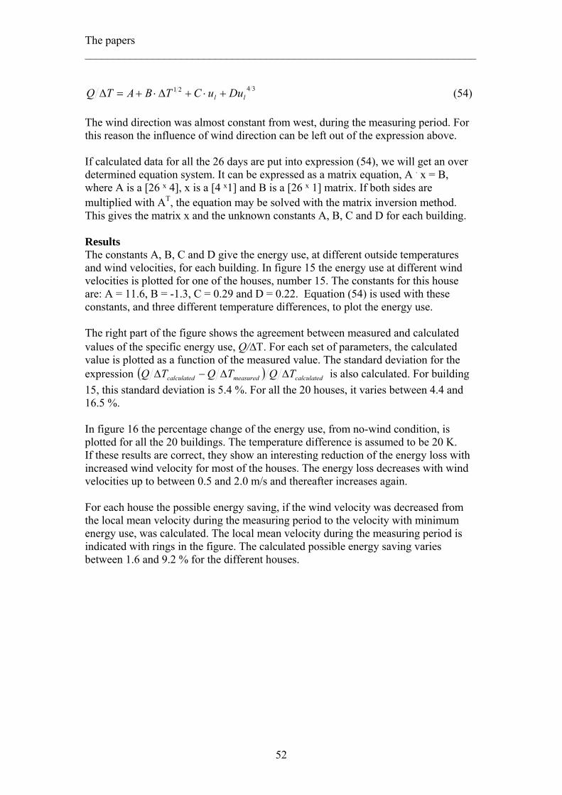
The papers _____________________________________________________________________

3421ll DuuCTBATQ +⋅+∆⋅+=∆ (54)

The wind direction was almost constant from west, during the measuring period. For this reason the influence of wind direction can be left out of the expression above. If calculated data for all the 26 days are put into expression (54), we will get an over determined equation system. It can be expressed as a matrix equation, A . x = B, where A is a [26 x 4], x is a [4 x1] and B is a [26 x 1] matrix. If both sides are multiplied with AT, the equation may be solved with the matrix inversion method. This gives the matrix x and the unknown constants A, B, C and D for each building. Results The constants A, B, C and D give the energy use, at different outside temperatures and wind velocities, for each building. In figure 15 the energy use at different wind velocities is plotted for one of the houses, number 15. The constants for this house are: A = 11.6, B = -1.3, C = 0.29 and D = 0.22. Equation (54) is used with these constants, and three different temperature differences, to plot the energy use. The right part of the figure shows the agreement between measured and calculated values of the specific energy use, Q/∆Τ. For each set of parameters, the calculated value is plotted as a function of the measured value. The standard deviation for the expression ( ) calculatedmeasuredcalculated TQTQTQ ∆∆−∆ is also calculated. For building 15, this standard deviation is 5.4 %. For all the 20 houses, it varies between 4.4 and 16.5 %. In figure 16 the percentage change of the energy use, from no-wind condition, is plotted for all the 20 buildings. The temperature difference is assumed to be 20 K. If these results are correct, they show an interesting reduction of the energy loss with increased wind velocity for most of the houses. The energy loss decreases with wind velocities up to between 0.5 and 2.0 m/s and thereafter increases again. For each house the possible energy saving, if the wind velocity was decreased from the local mean velocity during the measuring period to the velocity with minimum energy use, was calculated. The local mean velocity during the measuring period is indicated with rings in the figure. The calculated possible energy saving varies between 1.6 and 9.2 % for the different houses.

52

The papers _____________________________________________________________________

Figure 15. The result for house 15.

53

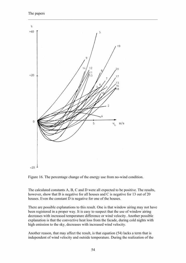
The papers _____________________________________________________________________

Figure 16. The percentage change of the energy use from no-wind condition. The calculated constants A, B, C and D were all expected to be positive. The results, however, show that B is negative for all houses and C is negative for 13 out of 20 houses. Even the constant D is negative for one of the houses. There are possible explanations to this result. One is that window airing may not have been registered in a proper way. It is easy to suspect that the use of window airing decreases with increased temperature difference or wind velocity. Another possible explanation is that the convective heat loss from the facade, during cold nights with high emission to the sky, decreases with increased wind velocity. Another reason, that may affect the result, is that equation (54) lacks a term that is independent of wind velocity and outside temperature. During the realization of the

54

The papers _____________________________________________________________________ study, the effort was to estimate all climate independent heat losses, e.g. hot water losses. However, there is one heat loss that wasn’t estimated and that is the heat loss to the soil and ground water under the building. For the split-level houses, also a part of the heat loss through the basement walls is climate independent. It is difficult to know if the results would have been different, with a constant term added to equation (54). The lack of it is, however, a possible explanation of the rather strange dip in the calculated heat loss that occurs at wind velocities of 1–2 m/s. One clear result from the study is the big importance that the behaviour of the occupants has. The difference in measured total energy use could be considerable between two identical houses. The study also show, in spite of some doubtful results, that the heat loss, and the airflow through the building, increases with both decreased outside temperature and increased wind velocity.

Paper 2. Ventilation of one family houses (1998) Objectives The previous work gave me an increased interest in how wind and buoyancy influences ventilation and infiltration. As a continuation, a series of calculations were performed on one-zone models of buildings, during the years 1983-84. Models with both a limited number of distinct leakage openings and with evenly spread leakages were tried. Some results of these latter calculations are presented in the chapter Airflow modelling. The calculations gave a sense of the climatic influence on the airflows in a building and how natural and mechanical driving forces are combined. The intention with the calculations was to construct a model for the airflows in buildings. The limited access to computer power, and computer software, at the time, made it difficult to fulfill these intentions. 10 years later, the computer evolution made it possible to restart the project. The new interest in natural, and hybrid, ventilation at the time also made it more important to learn about the ways that wind and outside temperature influence the building airflows. The paper “Ventilation of one family houses” describes results from a huge amount of computer simulations. Both natural, exhaust and supply-exhaust ventilation was studied, with different combinations of outside temperature, wind direction and wind velocity. This time a multi zone modelling was performed, with the computer program IDA and its airflow application MAE. The version used at the time, IDA Version 1.1, from 1995/96 (Bris Data 1996), could only make a model simulation for one set of parameters at a time. Since a new set of parameters had to put into the program, for each simulation, the number of possible parameter combinations was limited. For the preparation of this paper simulations of 3150 different combinations were performed. The air exchange rates in the bedrooms and in the living room, as well as the entire building, have been calculated. Method The studied building model is based on the assumptions of the IEA Annex 27 (Månsson 1996). In these assumptions, the building and leakage dimensions of two

55

The papers _____________________________________________________________________ different buildings are described. The chosen two storey one family house has an area of 83 m2. In the assumptions, the room areas are rounded, which has the consequence that the lower floor area is 38 m2 and the upper floor area is 45 m2. The room height is 2.5 m. Although this house is small, compared to most Swedish one family houses, it suits its purpose well since it consists of all the types of rooms that are of interest. The building is located along the north – south axis, see figure 17. The living room and bedrooms 1 and 2 are facing the south direction, while the other rooms are facing the north direction.

Figure 17. The model building. The values of the leakage openings in the building walls are based on the assumption of 2.5 air changes at 50 Pa pressure difference. In the present Swedish Building Code (Boverkets byggregler, BBR, (BFS 2002:19)), the maximum accepted airflow at 50 Pa pressure difference is 0.8 l/s and m2 surrounding area. The surrounding area is all outer walls, roof and floor. If the building is constructed with a concrete slab, the floor area may be neglected. The model building has a total surrounding area of 223 m2. If the floor area is excluded it is 179 m2. With these areas, the maximum accepted airflow in the Swedish Building Code corresponds to 2.92 and 2.34 air changes an

56

The papers _____________________________________________________________________ hour respectively. The assumed value of 2.5 air changes an hour may thus be reasonable. The mass flow rate through an opening may be calculated as

npCm ∆⋅=•

(23) where n is the flow exponent, ∆p is the pressure difference across the opening and C is the flow coefficient (Herrlin 1992). The assumed 2.5 air changes an hour at 50 Pa corresponds to 2.5 . 2.5 . 83 . 1.205/3600 = 0.1736 kg/s at 20 oC. The use of equation (60), with the assumed flow exponent n = 0.66 from the Annex 27 assumptions, gives a value of the total flow coefficient C for all the leakage openings.

)/(0131.0501736.0 66.0

66.066.0

.

PakgCpmC ==⇒

∆= (55)

The total flow coefficient is a measure of the total leakage area. This area is distributed as flow coefficients to the different rooms in proportion to each room’s relative floor area. The result of the distribution is shown in table 3. All leakage and supply openings are located on the south and north facades, except the two leakage openings in the upper hall, which are located on the east facade. No leakage openings are assumed in roof or floor or in interior walls, and the leakage openings are assumed to be located at two levels in each room, 0.625 and 1.875 m above the floor. It is notable that the flow coefficient used in the IDA-program is introduced as a constant. No correction for e.g. temperature is used. In all rooms with intended supply of outside air, i.e. living room and bedrooms, a supply opening is located 2 m above floor. The supply opening area is 80 cm2 in the living room and 40 cm2 in each bedroom. The mass flow rate through an opening may be calculated with equation (23). It may also be calculated with the help of the following expression.

nn pELAm ∆⋅

⋅⋅⋅=

•

424 ρ

(27)

When the opening size is given as an area, which is the case with supply, overflow and grille openings in the Annex 27 assumptions, the mass flow rate may be calculated with the expression for a sharp-edged orifice

ρρ pACm D

∆⋅⋅⋅⋅=

• 2 (19)

where CD is the discharge coefficient, which is often assumed as 0.6, and A is the area of the opening.

57

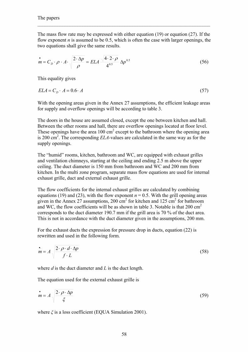
The papers _____________________________________________________________________ The mass flow rate may be expressed with either equation (19) or equation (27). If the flow exponent n is assumed to be 0.5, which is often the case with larger openings, the two equations shall give the same results.

5.05.04

242 pELApACm D ∆⋅⋅

=∆⋅

⋅⋅⋅=• ρ

ρρ (56)

This equality gives

AACELA D ⋅=⋅= 6.0 (57) With the opening areas given in the Annex 27 assumptions, the efficient leakage areas for supply and overflow openings will be according to table 3. The doors in the house are assumed closed, except the one between kitchen and hall. Between the other rooms and hall, there are overflow openings located at floor level. These openings have the area 100 cm2 except to the bathroom where the opening area is 200 cm2. The corresponding ELA-values are calculated in the same way as for the supply openings. The “humid” rooms, kitchen, bathroom and WC, are equipped with exhaust grilles and ventilation chimneys, starting at the ceiling and ending 2.5 m above the upper ceiling. The duct diameter is 150 mm from bathroom and WC and 200 mm from kitchen. In the multi zone program, separate mass flow equations are used for internal exhaust grille, duct and external exhaust grille. The flow coefficients for the internal exhaust grilles are calculated by combining equations (19) and (23), with the flow exponent n = 0.5. With the grill opening areas given in the Annex 27 assumptions, 200 cm2 for kitchen and 125 cm2 for bathroom and WC, the flow coefficients will be as shown in table 3. Notable is that 200 cm2 corresponds to the duct diameter 190.7 mm if the grill area is 70 % of the duct area. This is not in accordance with the duct diameter given in the assumptions, 200 mm. For the exhaust ducts the expression for pressure drop in ducts, equation (22) is rewritten and used in the following form.

LfpdAm

⋅∆⋅⋅⋅

=• ρ2.

(58)

where d is the duct diameter and L is the duct length. The equation used for the external exhaust grille is

ξρ pAm ∆⋅⋅

=• 2 (59)

where ξ is a loss coefficient (EQUA Simulation 2001).

58

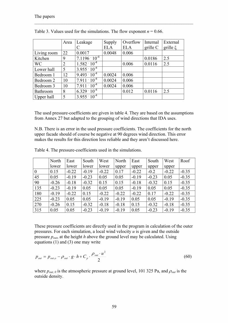
The papers _____________________________________________________________________ Table 3. Values used for the simulations. The flow exponent n = 0.66. Area Leakage

C Supply ELA

Overflow ELA

Internal grille C

External grille ξ

Living room 22 0.0017 0.0048 0.006 Kitchen 9 7.1196 . 10-4 0.0186 2.5 WC 2 1.582 . 10-4 0.006 0.0116 2.5 Lower hall 5 3.955 . 10-4 Bedroom 1 12 9.493 . 10-4 0.0024 0.006 Bedroom 2 10 7.911 . 10-4 0.0024 0.006 Bedroom 3 10 7.911 . 10-4 0.0024 0.006 Bathroom 8 6.329 . 10-4 0.012 0.0116 2.5 Upper hall 5 3.955 . 10-4 The used pressure-coefficients are given in table 4. They are based on the assumptions from Annex 27 but adapted to the grouping of wind directions that IDA uses. N.B. There is an error in the used pressure coefficients. The coefficients for the north upper facade should of course be negative at 90 degrees wind direction. This error makes the results for this direction less reliable and they aren’t discussed here. Table 4. The pressure-coefficients used in the simulations. North

lower East lower

South lower

West lower

North upper

East upper

South upper

West upper

Roof

0 0.15 -0.22 -0.19 -0.22 0.17 -0.22 -0.2 -0.22 -0.35 45 0.05 -0.19 -0.23 0.05 0.05 -0.19 -0.23 0.05 -0.35 90 -0.26 -0.18 -0.32 0.15 0.15 -0.18 -0.32 0.15 -0.35 135 -0.23 -0.19 0.05 0.05 0.05 -0.19 0.05 0.05 -0.35 180 -0.19 -0.22 0.15 -0.22 -0.22 -0.22 0.17 -0.22 -0.35 225 -0.23 0.05 0.05 -0.19 -0.19 0.05 0.05 -0.19 -0.35 270 -0.26 0.15 -0.32 -0.18 -0.18 0.15 -0.32 -0.18 -0.35 315 0.05 0.05 -0.23 -0.19 -0.19 0.05 -0.23 -0.19 -0.35 These pressure coefficients are directly used in the program in calculation of the outer pressures. For each simulation, a local wind velocity u is given and the outside pressure pout, at the height h above the ground level may be calculated. Using equations (1) and (3) one may write

2

2

,u

Chgpp outpoutooutout

⋅⋅+⋅⋅−=

ρρ (60)

where pout, 0 is the atmospheric pressure at ground level, 101 325 Pa, and ρout is the outside density.

59

The papers _____________________________________________________________________ The fans used in the exhaust and supply-exhaust cases, are assumed to give constant flow regardless of pressure difference, 10 l/s each from kitchen, bathroom and WC. This is according to the Annex 27 assumptions but not the case in reality. With a real fan, the airflow will vary with outside and inside pressures. The magnitude of variation is depending on the fan’s system curve. Simulations at different combinations of outside temperature, wind direction and wind velocity have been realized with three different ventilation systems; natural ventilation (passive stack ventilation), exhaust ventilation and supply-exhaust ventilation. With the mechanical ventilation systems, there have been no ventilation chimneys from kitchen, bathroom and WC. With supply-exhaust ventilation there has been no supply openings in living room and bedroom outer walls. In the older version of IDA, a constant uniform value of the inside temperature has to be used for each room. In this work, it has been set to 20 oC in all rooms. This work is a parameter study, but only parameters concerning the outdoor climate are studied. The number of possible combinations of these parameters made the variation of other parameters too time consuming. Only one configuration of openings, defined by position and opening area, is thus studied. The outside temperature has been varied in 2 oC steps between –30 and +18 oC. The wind direction has been varied in 45 o steps between 0 and 225 o and the wind velocity in 2 m/s steps between 0 and 12 m/s. With three different ventilation systems, 25 different outside temperatures, 6 different wind directions and 7 different wind velocities, 3150 different simulations are made altogether. For each combination of climatic conditions, the air exchange rates in the living room, in the bedrooms and in the entire building, have been calculated. The air exchange rate is defined as the volume airflow, at 20 oC, supplied directly from the outside divided by the room volume. This definition means that a room, with all its air supply coming from another room, has the air exchange rate 0. The airflow from the outside may enter either through the supply openings or through leakage openings. Results The requirements on minimum outside air supply in the Swedish Building Code, 0.35 l/s, m2 floor area, corresponds to an air exchange rate of 0.5 air changes an hour. The assumed exhaust flow with exhaust or supply-exhaust ventilation, 30 l/s, corresponds to an air exchange for the entire building of 0.52 air changes an hour. The results show that the Building Code requirement for the entire building always is exceeded when mechanical ventilation is used. With natural ventilation the air exchange is below that value at low wind velocities and/or high outside temperatures. Figure 18 shows the results at south wind. For other wind directions the results are very similar. The poor results at outside temperatures above 0 oC and at low wind velocities, indicate that the use of a help fan may be necessary at these conditions. The supply-grilles may also have to be closed at low outside temperatures and high wind velocities to reduce the ventilation rate.

60

The papers _____________________________________________________________________ Entire building, South wind, Passive stack ventilation

0

0,5

1

1,5

2

2,5

0 2 4 6 8 10 12

Wind speed (m/s)

Air

exch

ange

rate

-30

-26

-22

-18

-14

-10

-6

-2

2

6

10

14

18 Figure 18. Air exchange rate in the entire building at different outside temperatures. Natural ventilation and wind from south. When it comes to the air exchange in specific rooms, the results are different. The resulting air exchange with exhaust or natural ventilation is very depending on the wind direction. Figures 19 and 20 show the air exchange in bedroom 1 at north wind, i.e. when the room is on the leeside.

Bedroom 1, North wind, Exhaust ventilation

0 0,1 0,2 0,3 0,4 0,5 0,6 0,7

0 2 4 6 8 10 12

Wind speed (m/s)

Air

exch

ange

rate

-30

-26

-22

-18

-14

-10

-6

-2

2

6

10

14

18 Figure 19. Air exchange in bedroom 1 at different outside temperatures. Exhaust ventilation and wind from north.

61

The papers _____________________________________________________________________

Bedroom 1, North wind, Passive stack ventilation

0 0,2 0,4 0,6 0,8

1 1,2

0 2 4 6 8 10 12

Wind speed (m/s)

Air

exch

ange

rate

-30

-26

-22

-18

-14

-10

-6

-2

2

6

10

14

18 Figure 20. Air exchange in bedroom 1 at different outside temperatures. Natural ventilation and wind from north. If the specific room is on the leeward side, increasing wind velocity tends to draw air out of the room, and thus decrease the supply of outside air. This is what happens in the case with exhaust ventilation, figure 19. When passive stack ventilation is used, the pressure inside the building is decreased more than the pressure on the leeward facade. The reason for this is the ventilation chimneys. With increasing wind velocity the airflow through the chimneys increase. This means that the air exchange doesn’t decrease with increasing wind. It actually increases somewhat. With exhaust ventilation, on the other hand, the constant exhaust airflows from “humid” rooms give a constant reduction of the pressure inside the building. The results for bedroom 3 are the same as for bedroom 1 with exhaust ventilation. With passive stack ventilation, however, the air exchange is decreasing with increasing wind velocity if bedroom 3 is on the leeward side, see figure 21. This is the case when the outside temperature is below zero. The reason why bedroom 3 performs worse at wind from south, than bedroom 1 does at wind from north, is the unequal spread of opening areas between the facades. The building is almost to consider as a terraced one with two exposed facades. Since all “humid” rooms, without supply openings, are located at the north facade, this facade contains fever openings. With wind from south the pressure inside the building doesn’t decrease as much as it does with wind from north. The wind against the facades indeed increases the inside pressure and counteracts the flow through the chimneys, that decreases the inside pressure. It is thus more difficult to supply bedroom 3 with outside air, at south wind, then it is to supply bedroom 1 at north wind.

62

The papers _____________________________________________________________________

Bedroom 3, South wind, Passive stack ventilation

0 0,2 0,4 0,6 0,8

1 1,2

0 2 4 6 8 10 12

Wind speed (m/s)

Air

exch

ange

-30

-26

-22

-18

-14

-10

-6

-2

2

6

10

14

18 Figure 21. Air exchange in bedroom 3 at different outside temperatures. Natural ventilation and wind from south. With supply-exhaust ventilation, this phenomenon doesn’t occur and the required air exchange is exceeded in all rooms at all wind directions. The assumed tightness of the building is low enough to make the effect of wind and temperature difference negligible. This study is a pure parameter study, in which the affect of different parameter combinations is studied. However, no consideration is taken to the stochastic variation of these parameter values. The combination of 0 oC outside and 2 m/s wind velocity is, as an example, much more common than –30 oC and 12 m/s.

Paper 3. Annual variation of air distribution in a cold climate (2003) Objectives From the previous study, it is difficult to draw any conclusions about the whole year performance of different ventilation systems. The influence of opening position and size is also unknown. This study aims to a deeper understanding of this for a naturally ventilated building. It is focused on the influence of different possible measures to increase the ventilation flows. The airflows in all rooms of the building are studied. Method The new program version of the multi zone program IDA, IDA Climate and Energy 3.0, makes it possible to run simulations for each hour during a whole year. Climate files for different places may be used as input data. For this paper, a climate file for the Swedish city Östersund, generated from ASHRAE IWEC 1.1 Weather Files is used (ASHRAE 2001). The possibility to simulate the behaviour of the ventilation system for a whole year, in only one simulation run, makes it possible to vary other parameters than the climate. Starting from a basic configuration, of opening sizes and positions, different

63

The papers _____________________________________________________________________ combinations of opening sizes are studied. The opening sizes described below determine the basic configuration. Basically the same model building as in the previous paper is used. There are however some differences between the models. This means that it is difficult to directly compare absolute calculated values between the papers. One difference is that the size of the rooms is following the drawing of the building, in the Annex 27 assumptions, instead of the rounded areas given. Thus, each floor has the area 42 m2. The total building volume is thus bigger and each room has a different relative size. The sizes of the leakage openings are therefore different. They are also fed into the simulation program as ELA-values, which may be seen in table 5. The conversion from flow coefficients, C, to efficient leakage values, ELA, is made with the help of equation (57). The input parameter for the internal exhaust grille is here the loss coefficient ξ and the mass flow is calculated with equation (59). Also for the external exhaust grille, the loss coefficient ξ is the input to the program and equation (59) is used. The calculation of the mass flow through the exhaust duct is rather different in IDA Climate and Energy compared to the MAE application of IDA version 1.1. The more refined equation used for the mass flow rate is

ρξ

⋅⋅+

∆=

•

22 21

Ac

pm

temp

(61)

where ctemp is a temporary parameter defined as

27.3

log72

1 ⋅⎟⎟⎠

⎞⎜⎜⎝

⎛+

⋅⋅

⋅⋅⋅= K

de

Ld

Ach

htemp

ρ (62)

and K1 is 3.289 . 10-3 when Re is < 4 000 (laminar flow) 5.74/Re0.9 when Re is > 4 000 (turbulent flow) e is the surface roughness of the duct inner surface and dh is the hydraulic diameter (similar to the diameter d when the duct is circular). (EQUA Simulation 2001) In this study, the airflow through the open kitchen door (and living room and bedroom doors when open) is calculated. IDA uses a model for bi-directional flow through vertical rectangular openings. Density gradients in connected zones are neglected.

64

The papers _____________________________________________________________________ Table 5. Values used for the simulations. The flow exponent n = 0.66. Area Leakage

ELA Supply ELA

OverflowELA

Internal grille ξ

External grille ξ

Living room 25 15.7438 . 10-4 0.0048 0.006 Kitchen 8.7 5.566 . 10-4 10 2.5 WC 3.8 2.3854 . 10-4 0.006 10 2.5 Lower hall 6.5 4.2938 . 10-4 Bedroom 1 10 6.3611 . 10-4 0.0024 0.006 Bedroom 2 10 6.3611 . 10-4 0.0024 0.006 Bedroom 3 10 6.3611 . 10-4 0.0024 0.006 Bathroom 7.5 4.7709 . 10-4 0.012 10 2.5 Upper hall 6.5 4.1347 . 10-4 The pressure coefficients used for this paper differ from the earlier presented, see table 6. With the new IDA version, only one value per facade is possible to define. A mean value of the values for lower and upper part in table 4 is therefore used. The before mentioned error in table 4 is also corrected. Besides this, the values have been doubled compared to table 4. The reason for this is that the pressure-coefficients, given in the Annex 27 assumptions, are associated with meteorological wind data. These are normally given for the height 10 m above the ground. Since the wind velocities used in IDA are transformed to a local wind velocity at 6 m height, before using them for pressure calculations, the pressure-coefficients have to be increased. A wind profile for an urban area is used in the simulations (Bring, Sahlin et al. 1999) which gives the wind velocity at 6 m height as

metmet uuu ⋅=⋅⎟⎠⎞

⎜⎝⎛⋅= 59.010667.0

25.0

(63)

where umet is the meteorological wind velocity and 0,25 is the wind profile exponent n. This means that the pressure-coefficients should be increased 1/0.592 = 2.87 times. This corresponds to the recommendation on a 2–3 times increase, given in the Annex 27 assumptions. However, due to the uncertain values, a doubling of the coefficients is used in this work.

65

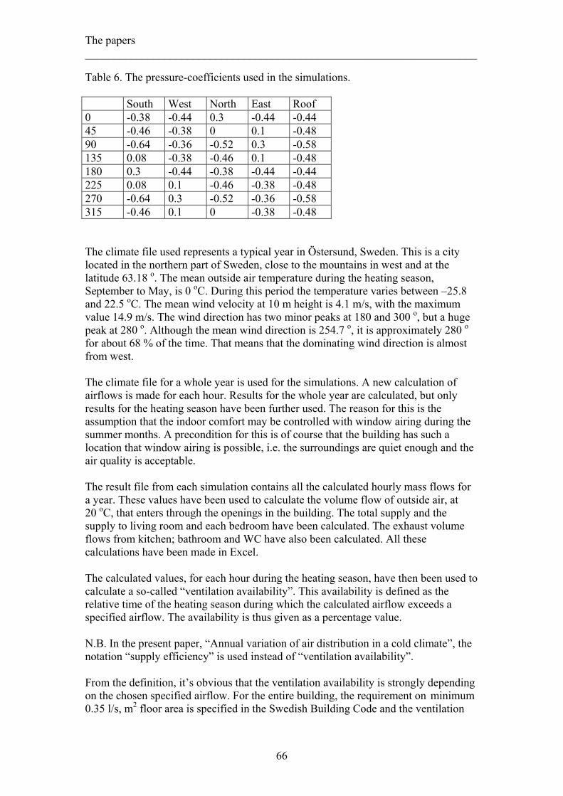
The papers _____________________________________________________________________ Table 6. The pressure-coefficients used in the simulations. South West North East Roof 0 -0.38 -0.44 0.3 -0.44 -0.44 45 -0.46 -0.38 0 0.1 -0.48 90 -0.64 -0.36 -0.52 0.3 -0.58 135 0.08 -0.38 -0.46 0.1 -0.48 180 0.3 -0.44 -0.38 -0.44 -0.44 225 0.08 0.1 -0.46 -0.38 -0.48 270 -0.64 0.3 -0.52 -0.36 -0.58 315 -0.46 0.1 0 -0.38 -0.48 The climate file used represents a typical year in Östersund, Sweden. This is a city located in the northern part of Sweden, close to the mountains in west and at the latitude 63.18 o. The mean outside air temperature during the heating season, September to May, is 0 oC. During this period the temperature varies between –25.8 and 22.5 oC. The mean wind velocity at 10 m height is 4.1 m/s, with the maximum value 14.9 m/s. The wind direction has two minor peaks at 180 and 300 o, but a huge peak at 280 o. Although the mean wind direction is 254.7 o, it is approximately 280 o for about 68 % of the time. That means that the dominating wind direction is almost from west. The climate file for a whole year is used for the simulations. A new calculation of airflows is made for each hour. Results for the whole year are calculated, but only results for the heating season have been further used. The reason for this is the assumption that the indoor comfort may be controlled with window airing during the summer months. A precondition for this is of course that the building has such a location that window airing is possible, i.e. the surroundings are quiet enough and the air quality is acceptable. The result file from each simulation contains all the calculated hourly mass flows for a year. These values have been used to calculate the volume flow of outside air, at 20 oC, that enters through the openings in the building. The total supply and the supply to living room and each bedroom have been calculated. The exhaust volume flows from kitchen; bathroom and WC have also been calculated. All these calculations have been made in Excel. The calculated values, for each hour during the heating season, have then been used to calculate a so-called “ventilation availability”. This availability is defined as the relative time of the heating season during which the calculated airflow exceeds a specified airflow. The availability is thus given as a percentage value. N.B. In the present paper, “Annual variation of air distribution in a cold climate”, the notation “supply efficiency” is used instead of “ventilation availability”. From the definition, it’s obvious that the ventilation availability is strongly depending on the chosen specified airflow. For the entire building, the requirement on minimum 0.35 l/s, m2 floor area is specified in the Swedish Building Code and the ventilation

66

The papers _____________________________________________________________________ availability is based on that. For the different rooms, however, there are only recommendations in the Building Code (Boverket 1995a). A consulting engineer, who is to design a ventilation system, usually starts from the total required airflow for the building and then distributes this airflow to the different rooms. This distribution may e.g. be based on the Building Code recommendations. The present model building has a total are of 88 m2 which means that the minimum supply (and exhaust) airflow is 0.35 . 88 l/s = 30.8 l/s. For bedrooms, the recommendation is 4 l/s and bed. For kitchen, bathroom and WC, the recommendation is 10 l/s each (without forced airflow). Based on this, a possible airflow design may be made. These values, shown in table 7, are used as specified airflows when determining the ventilation availability in this paper. Table 7. Specified airflows, used at calculation of ventilation availabilities. Supply air (l/s) Exhaust air (l/s) Living room 8.0 Kitchen 10.8 Bedroom 1 7.4 Bathroom 10.0 Bedroom 2 8.0 WC 10.0 Bedroom 3 7.4 Total building 30.8 30.8 Bedroom 2 is assumed to have larger design airflow than bedroom 1, although the floor areas are equal, because it is assumed to be a master bedroom with two beds. For this paper, these design airflows are used as specified airflows when calculating the ventilation availability. This choice of airflows give ventilation availabilities, for kitchen and bedrooms 1 and 3, that are worse than if the recommended values for these rooms had been chosen instead. However, if two persons or more use a bedroom, the recommended airflow for a bedroom is higher than the used one. In that case, the ventilation availability should be even lower. The living room on the other hand gets a better value than it should, since 8.0 l/s is less than 0.35 l/s, m2 living room floor area. The ventilation availability has been calculated for the entire building as well as for the separate rooms, at different opening configurations. Only natural ventilation (passive stack ventilation) is studied in this paper. A basic configuration of the building has the opening areas according to table 5, supply openings at 2 m level in living room and bedrooms, open kitchen door but doors to other rooms closed and ventilation chimneys ending 2.5 m above the upper ceiling. Results The calculated ventilation availabilities, with the basic configuration, are quite low for some rooms and very low for others. The entire building has a ventilation availability of 38.8 %, i.e. the minimum requirement in the Swedish Building Code is fulfilled for less than half the heating season.

67

The papers _____________________________________________________________________ The kitchen is the only room that has an acceptable availability, 96 %. This is entirely due to the open door between kitchen and hall, which decreases the necessary under-pressure that the ventilation chimney has to create. For the bathroom and the WC, with closed doors, the flow resistance in the overflow opening is too high. The ventilation availability in these rooms is less than 1 %. The “dry” rooms have availabilities varying between 57 %, for the living room, and approximately 2 % for the bedrooms. The availabilities for the later rooms are lower, because they have smaller supply opening areas but the same overflow openings to the hall. In the basic configuration, the supply openings in the bedrooms and living room are located 2 m above floor level, i.e. in the upper frame of the window. This is a common location for supply openings in natural and exhaust ventilated buildings in Sweden. When a supply opening is located in a room at the upper floor it may, however, end up below the neutral level. This may happen even with lower positions than 2 m (Maeyens and Janssens 2003). To minimize this risk, the supply openings on the upper floor shall be located as low as possible (Bergsøe, Blomsterberg et al. 1996). One shall however be aware, that a lowering of the supply openings by itself lowers the neutral level. A change of the supply opening position, to 0.1 m above the floor level in the bedrooms, increases the ventilation availability in these rooms to 3.6, 3.0 and 3.9 % respectively. These values are still very low. For the following calculations, the basic configuration implies this supply opening position. Starting with the basic configuration, new configurations have been established and the resulting ventilation availabilities determined. An increase of the ventilation chimney height increases the buoyancy forces and thus the airflows, see figure 22. The increase is largest for the rooms with initial low ventilation availabilities. One may, however, observe that even such a big addition to the chimney height, as 6 m, isn’t, in itself, enough to give acceptable availabilities. Such a big addition, to the basic 2.5 m above the upper ceiling, is also difficult to defend from an architectural point of view. Instead of increasing the chimney height, the ventilation availabilities may be increased by either opening inner doors in the building or/and increasing opening areas. The effect of larger opening areas has been calculated with

a) all doors, except kitchen door, closed b) living room door open c) living room and bedroom doors open

68

The papers _____________________________________________________________________

0

20

40

60

80

100

120

0 1 2 3 4 5 6 7

Extra chimney height (m)

Vent

ilatio

n av

aila

bilit

y (%

)Living roomBedroom 1, 2Bedroom 3KitchenWCBathroom

Figure 22. Influence on the ventilation availability from increasing chimney height. For each case, the ventilation availability is calculated for four different opening size configurations. These are:

basic opening area supply openings to bedrooms doubled overflow openings to bedrooms doubled and overflow openings to WC/bathroom doubled

The result of case a) is shown in figure 23. As shown in the figure, the doubling of the supply openings to bedrooms is most effective in improving the availabilities for the rooms with the lowest initial values.

0.0

20.0

40.0

60.0

80.0

100.0

120.0

Vent

ilatio

n av

aila

bilit

y (%

)

Living room 52.2 46.8 48.8 54.8

Bedroom 1, 2 3.6 9.9 6.6 3.9

Bedroom 3 3.9 16.4 10.0 4.1

Kitchen 97.7 98.2 98.1 97.1

WC 0.2 0.7 0.4 0.9

Bathroom 1.3 3.0 2.2 2.7

1 2 3 4

Figure 23. The ventilation availability in different rooms at different opening configurations. Living room door closed. 1) basic opening area, 2) supply openings to bedrooms doubled, 3) overflow openings to bedrooms doubled and 4) overflow openings to WC/bathroom doubled.

69

The papers _____________________________________________________________________ The result of case b) is shown in figure 24. The opening of the living room door improves the result for the living room (as expected), bathroom and WC, but deteriorates the result for the bedrooms. An open living room door, which is common in Swedish family houses, thus makes the ventilation of the bedrooms even worse. This is due to the fact that it’s easier, for the supply air, to enter the building through the openings in the living room than in the bedrooms, when the living room door is open.

0.0

20.0

40.0

60.0

80.0

100.0

120.0

Vent

ilatio

n av

aila

bilit

y (%

)

Living room 96.7 95.9 96.2 96.8

Bedroom 1, 2 2.6 4.7 3.7 2.8

Bedroom 3 2.7 8.1 5.3 2.8

Kitchen 98.7 98.9 98.8 98.6

WC 1.1 1.8 1.4 4.0

Bathroom 5.8 9.2 7.9 11.0

1 2 3 4

Figure 24. The ventilation availability in different rooms at different opening configurations. Living room door open. 1) basic opening area, 2) supply openings to bedrooms doubled, 3) overflow openings to bedrooms doubled and 4) overflow openings to WC/bathroom doubled. Figure 25 gives a more detailed picture of how the ventilation availabilities for the bedrooms change when the living room door is opened and the basic configuration is valid. Figure 26 finally shows the result if also the bedroom doors are open. Open bedroom doors, together with doubling of the supply opening areas in the bedrooms, may increase the ventilation availability to between 27.0 and 55.3 % for the bedrooms. A doubling of these areas means an increase from 40 cm2 to 80 cm2 per room. The availabilities for bathroom and WC are still very low.

70

The papers _____________________________________________________________________

00.5

11.5

22.5

33.5

44.5

1 2 3

Vent

ilatio

n av

aila

bilit

y (%

)

ClosedOpen

Figure 25. The effect on ventilation availability from opening of the living room door. Bedrooms 1, 2 and 3.

0,0

20,0

40,0

60,0

80,0

100,0

120,0

Supp

ly e

ffic

ienc

y (%

)

Living room 95,0 90,7 95,9

Bedroom 1, 2 6,0 27,0 7,7

Bedroom 3 14,3 55,3 17,1

Kitchen 98,9 99,2 98,9

WC 2,2 5,3 8,1

Bathroom 10,6 18,7 17,8

1 2 3

Figure 26. The ventilation availability in different rooms at different opening configurations. Living room and bedroom doors open. 1) basic opening area, 2) supply openings to bedrooms doubled and 3) overflow openings to WC/bathroom doubled. Opening of the bedroom doors is a measure that may be taken to improve the airflow to these rooms. A ventilation system shall however be able to fulfill the requirements even with closed doors. As shown in figures 22 – 26, one separate measure isn’t enough. All opening areas have to be increased and even more than doubled. There may still be necessary to complement the natural forces with mechanical aid, in order to achieve acceptable ventilation availabilities.

71

The papers _____________________________________________________________________ For kitchen, bathroom and WC, the relative time of the heating season during which the airflow has a wrong direction, has been calculated as well. The air flows in the wrong direction when it flows from the “humid” room out into the hall. So far, these calculated values haven’t been analyzed. The energy use during the whole year is also calculated for each simulation. It is separated into electric energy, for e.g. lighting, and heating energy for the radiators. These calculated values have so far not been further studied.

Paper 4. Stack ventilation of rooms with closed doors (2004) Objectives The previous paper showed that the studied measures, e.g. change of opening areas or chimney height, were unable to give sufficient ventilation availabilities when used separately. This paper thus aims to study the combinations of different measures. In the previous paper, a rather severe condition was used for the determination of the ventilation availabilities for the different rooms. That was the design airflow for each room. In this paper, the ventilation availability is instead based on the recommended minimum airflows in the Building Code. Both natural and exhaust ventilation is studied. Model The building model and used climate file are the same as in the previous paper. Ventilation availabilities are calculated for the heating season. They are based on the minimum recommended airflows in the Swedish Building Code. For the living room, the airflow is based on the requirement of minimum 0.35 l/s, m2 floor area. The specified airflows used are seen in table 8. Two values are used for the bedrooms, depending on the number of occupants. If the bedroom is used as a master bedroom, the value is 8 instead of 4 l/s. Results with the higher value used are not presented in the paper. Bedroom 1 and 2 are treated as equal with the same ventilation availability. The use of different specified airflows means that ventilation availabilities can’t be directly compared between this and the previous paper. Table 8. Specified airflows used for the calculation of ventilation availability. Supply air (l/s)

Exhaust air (l/s)

Living room 8.8 Kitchen 10.0 Bedroom 1 4.0 8.0 Bathroom 10.0 Bedroom 2 4.0 8.0 WC 10.0 Bedroom 3 4.0 8.0 Total building 30.8 30.8 As a start for the simulations, a basic configuration for the building is assumed. It’s almost the same basic configuration as used in the last paper, but with supply openings in bedrooms at 0.1 m level.

72

The papers _____________________________________________________________________ Results The ventilation availability for bedroom 3 is higher than for bedroom 1, and the similar bedroom 2. This is the case with all studied configurations and was a result of the previous paper as well. The only difference between the rooms is the direction; bedroom 3 is located towards north and the other two towards south. The explanation is the same as the one mentioned in connection with the paper “Ventilation of one family houses”. In that study, bedroom 3 had lower supply airflow with wind from south than bedroom 1 with wind from north. The reason for that was the uneven spread of openings between south and north facade. The same reason makes it easier for the supply air to enter bedroom 3 at north wind than to enter bedroom 1, and 2, at south wind. Although the mean wind direction during the heating season is 254.7 o, the median direction is 279 o, see also the cumulative distribution in figure 27. This indicates longer periods with wind from north than from south. The mean wind velocity, with wind directions in the interval west-north-east, is also slightly higher than in the interval east-south-west, 4.14 m/s compared to 4.02 m/s. This small difference means that bedroom 3 will be better ventilated than bedrooms 1 and 2.

Figure 27. Cumulative distribution of wind direction during the heating season. The results of the different studied configurations are shown in table 9.

73

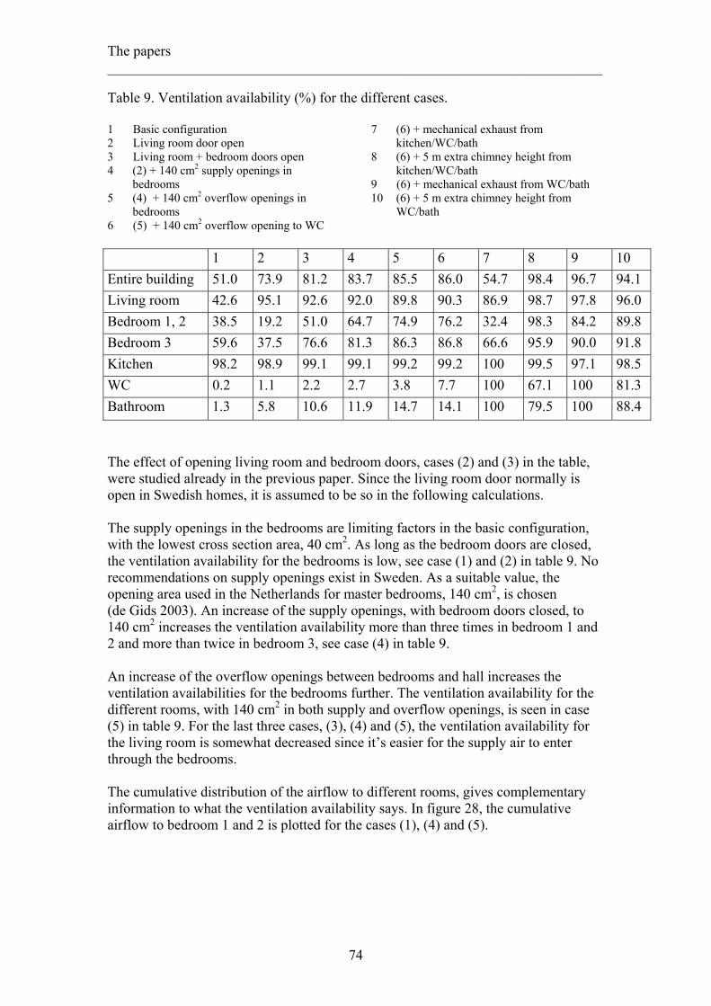
The papers _____________________________________________________________________ Table 9. Ventilation availability (%) for the different cases. 1 Basic configuration 2 Living room door open 3 Living room + bedroom doors open 4 (2) + 140 cm2 supply openings in

bedrooms 5 (4) + 140 cm2 overflow openings in

bedrooms 6 (5) + 140 cm2 overflow opening to WC

7 (6) + mechanical exhaust from kitchen/WC/bath

8 (6) + 5 m extra chimney height from kitchen/WC/bath

9 (6) + mechanical exhaust from WC/bath 10 (6) + 5 m extra chimney height from

WC/bath

1 2 3 4 5 6 7 8 9 10 Entire building 51.0 73.9 81.2 83.7 85.5 86.0 54.7 98.4 96.7 94.1 Living room 42.6 95.1 92.6 92.0 89.8 90.3 86.9 98.7 97.8 96.0 Bedroom 1, 2 38.5 19.2 51.0 64.7 74.9 76.2 32.4 98.3 84.2 89.8 Bedroom 3 59.6 37.5 76.6 81.3 86.3 86.8 66.6 95.9 90.0 91.8 Kitchen 98.2 98.9 99.1 99.1 99.2 99.2 100 99.5 97.1 98.5 WC 0.2 1.1 2.2 2.7 3.8 7.7 100 67.1 100 81.3 Bathroom 1.3 5.8 10.6 11.9 14.7 14.1 100 79.5 100 88.4 The effect of opening living room and bedroom doors, cases (2) and (3) in the table, were studied already in the previous paper. Since the living room door normally is open in Swedish homes, it is assumed to be so in the following calculations. The supply openings in the bedrooms are limiting factors in the basic configuration, with the lowest cross section area, 40 cm2. As long as the bedroom doors are closed, the ventilation availability for the bedrooms is low, see case (1) and (2) in table 9. No recommendations on supply openings exist in Sweden. As a suitable value, the opening area used in the Netherlands for master bedrooms, 140 cm2, is chosen (de Gids 2003). An increase of the supply openings, with bedroom doors closed, to 140 cm2 increases the ventilation availability more than three times in bedroom 1 and 2 and more than twice in bedroom 3, see case (4) in table 9. An increase of the overflow openings between bedrooms and hall increases the ventilation availabilities for the bedrooms further. The ventilation availability for the different rooms, with 140 cm2 in both supply and overflow openings, is seen in case (5) in table 9. For the last three cases, (3), (4) and (5), the ventilation availability for the living room is somewhat decreased since it’s easier for the supply air to enter through the bedrooms. The cumulative distribution of the airflow to different rooms, gives complementary information to what the ventilation availability says. In figure 28, the cumulative airflow to bedroom 1 and 2 is plotted for the cases (1), (4) and (5).

74

The papers _____________________________________________________________________

Figure 28. Cumulative distribution of air supply to bedroom 1 and 2. Basic configuration with living room door open (*), with 140 mm2 supply openings in bedrooms (x) and with 140 cm2 supply and overflow openings ( ). The flatter and lower forms of the last two curves indicate a higher probability for high airflows in these cases. Increasing of the supply openings with 250 % (from 40 to 140 cm2) is of course most important, as shown in the figure. Compared to that, the 40 % increase of the overflow openings has a smaller effect. Increase of the overflow opening to the WC to 140 cm2 as well, increases the exhaust flow from the WC, see case (6) in table 9, while the airflows to the other rooms remain almost the same. The overflow opening to the bathroom isn’t changed since it’s already 200 cm2. With all these measures taken, the results are acceptable for the entire building and for the bedrooms, but still real poor for the WC and the bathroom. The main reason for the poor results is the open door to the kitchen. The lack of flow resistance in that door opening makes the exhaust through the kitchen chimney dominate the flow through the building. 64 % of the total supply flow to the building leaves it through the kitchen chimney with case (6). This dominance decreases the pressure in the hall in such a way that the exhaust flow through the chimneys in WC and bathroom is counteracted. The ventilation of the WC and bathroom is a problem, with all the cases (1) to (6). Two ways to increase it have been studied. The first is to use mechanical exhaust from all “humid” rooms; kitchen, WC and bathroom, the other is to increase the height of the ventilation chimneys. A constant mechanical exhaust from the “humid” rooms, i.e. a conventional exhaust ventilation system, of course increases the ventilation availabilities for WC and

75

The papers _____________________________________________________________________ bathroom; see case (7) in table 9. But, at the same time this measure lowers the availabilities for living room and bedrooms. This is because a constant exhaust flow from the kitchen doesn’t utilize the strong stack effect that the kitchen chimney gives at low outside temperatures. The increase in exhaust flow from WC and bathroom is too small to compensate for the decreased flow from the kitchen. Independent of used configuration, the air pressures are lower at the second floor than at the first. But if the pressures are adjusted for the hydrostatic pressure difference, the pressure is lower at the first floor and there is always airflow from the second floor and down. This is due to the fact that two of the “humid” rooms, with equipment for exhaust flow, are located on the bottom floor. The use of a constant mechanical exhaust flow from all “humid” rooms increase the pressures in all rooms a bit (less than 1 Pa), most in kitchen and living room and least in the WC. This leads to decreased exhaust airflow from the kitchen. The mean flow during the heating season changes from 27.2 to 10.0 l/s. In spite of this, the ventilation availability for the kitchen is better with mechanical exhaust, due to the fact that the exhaust flow never goes below the constant value. The exhaust flows from WC and bathroom increase with mechanical exhaust, leading to higher ventilation availabilities for these rooms. This increase is however too small to compensate for the decreased flow from the kitchen, why the availabilities for the bedrooms decrease. Higher ventilation chimneys from the “humid” rooms may be used instead of mechanical exhaust. The objective must be to give a pressure in the WC and bathroom that is equal to what the mechanical fan gives, leading to similar airflows. Figure 29 shows the cumulative pressure distribution in the WC for 0, 3 and 5 m extra chimney height and for case (7) with mechanical exhaust from all “humid” rooms. A brief look at the distribution indicates that, for a major part of the year, both 3 and 5 m extra chimney height gives lower pressure than the mechanical exhaust. Also the mean pressures in bathroom and WC indicate that higher ventilation chimneys could replace the mechanical exhaust. It’s approximately 2.6 Pa lower, during heating season, with 5 m higher chimneys than with mechanical exhaust.

76

The papers _____________________________________________________________________

Figure 29. Pressure distribution in WC with extended chimney height compared to mechanical exhaust from WC/bathroom. ◊ = mechanical exhaust, o = 0 m, x = 3 m and □ = 5 m extra chimney height. Pressure relative to 100 000 Pa. Case (8) in table 9 shows that 5 m extra chimney height gives higher ventilation availabilities than the mechanical exhaust. But - this is not the fact for WC and bathroom, for which rooms the ventilation availabilities are much lower. A closer look at the cumulative pressure distribution shows that the solution with higher chimneys, for a shorter period gives much higher pressures than the mechanical exhaust. During this period the airflow decreases strongly leading to very low ventilation availability. In figure 30, the cumulative distribution of the airflow from hall to WC is plotted for cases (7) and (8). The figure shows a big difference between the two cases. Although the pressure distributions are quite similar, the flow with mechanical exhaust is almost constant while it varies a lot with 5 m extra chimneys.

77

The papers _____________________________________________________________________

Figure 30. Airflow between hall and WC with ◊ = case (7) and □ = case (8). With higher ventilation chimneys, the mean airflow is higher but there are periods with very low, even negative, airflows, leading to lower ventilation availabilities for WC and bathroom. Both cases (7) and (8) give unacceptable low ventilation availabilities for some rooms. With mechanical exhaust, that concerns both the entire building and the bedrooms, and with higher ventilation chimneys, the WC and the bathroom. In both cases, the performance of the system may be improved by excluding the kitchen from changes, i.e. by keeping the kitchen ventilated by a chimney with basic height. If a constant mechanical exhaust is used only from WC and bathroom, the airflows will be sufficient from these rooms and increased in the other. The overall result is much better than with case (7), see case (9) in table 9. The pressures in bathroom and WC decrease somewhat in this case, while they are unchanged in the rest of the building. If extended chimney heights are used only from WC and bathroom, the availabilities are improved for these rooms. They decrease somewhat for the rest of the building, but are still sufficient, see case (10) in table 9. The reason for the better results, with excluded kitchen, is that the use of increased exhausts from all “humid” rooms decreases the pressures not only in WC and bathroom. The pressures are also lowered in the kitchen and all the other rooms. Although these pressures don’t decrease as much as in the WC and bathroom, the exhaust flow from the kitchen increases much more than the flows from WC and bathroom. This is due to the low flow resistance in the kitchen door. Increased

78

The papers _____________________________________________________________________ exhaust from the kitchen only counteracts the exhaust flow from WC and bathroom and is really not necessary for the ventilation of the kitchen. This last results are acceptable even if the availability for the WC is a bit low. The case however shows that it is possible to achieve an acceptable level of ventilation with passive stack ventilation. The results are however valid only for the climate of the northern city Östersund. This climate is favourable for natural ventilation with it’s low outside temperatures and relative high wind velocities. In order to control the function of the ventilation system in other climates, simulations with case (10) have been performed for two additional climate files. These are climate files for Stockholm (latitude 59.35o) and Gothenburg (latitude 57.7o). The ventilation availabilities have been calculated for the same period as in Östersund, 9 months, even though the heating season is shorter at these locations. The results with these climate files are presented in table 10. As expected, the results for the more south located cities are not as good as for Östersund. One may also notice that the ventilation availability for bedroom 3 is lower than the availability for bedroom 1, 2. Thus the opposite condition compared to Östersund. The different dominating wind directions explain this. In Stockholm and Gothenburg, the average wind direction during the heating season is approximately from south (193.0 and 159.0 o respectively), while the average wind direction in Östersund is from west (254.7 o). Table 10. Ventilation availabilities for three locations, Östersund, Stockholm and Gothenburg. Case (10). Östersund Stockholm GothenburgWhole building 94.1 90.1 87.7 Living room 96.0 92.9 91.2 Bedroom 1, 2 89.8 89.9 88.6 Bedroom 3 91.8 74.6 65.6 Kitchen 98.5 97.2 95.5 WC 81.3 70.0 67.7 Bathroom 88.4 79.2 76.5 The cumulative distribution of the supply airflow to bedroom 1, 2 is shown in figure 31. Although the ventilation availability for bedroom 1, 2 is lowest in the Gothenburg climate, the number of days with high airflows is much higher here than at the other two locations. Since the required airflow for the calculation of the ventilation availability is 4 l/s, these high airflows don’t affect the availability. The reason for the high airflows, are the high wind velocities that are frequent in the Gothenburg climate. Although the mean velocity during the heating season is approximately the same as in Östersund, the highest velocity is 20 m/s compared to 14.9 m/s in Östersund (Stockholm has lower velocities).

79

The papers _____________________________________________________________________

Figure 31. Ventilation availability for bedroom 1, 2. Östersund (*), Stockholm (o) and Gothenburg (x). If passive stack ventilation is to be used in a more southern climate, the building configuration has to be changed, either with even higher ventilation chimneys or with larger opening areas. According to the results from simulations, passive stack ventilation of a two storey, detached one family house is possible in a northern climate. A precondition for this is however the use of very high ventilation chimneys from the “humid” rooms. This of course affects the building appearance and may be hard for an architect to accept. Due to the importance of low flow resistance in the ducts, separate ventilation chimneys are needed. Only if the kitchen, bathroom and WC are closely placed in the building, the chimneys may be combined to one unit. If high ventilation chimneys aren’t accepted, a hybrid ventilation system, with mechanical exhaust from WC/bathroom, is a possible solution. Another necessary condition is that the openings in inner and outer walls have large enough area. In this paper, opening areas up to 140 cm2 have been assumed (except the 200 cm2 opening to the bathroom). Even bigger openings would probably increase the supply availabilities but may lead to stability problems. The paper also shows the importance of designing the ventilation system according to the climatic conditions. Different locations have different dominating wind directions, mean wind velocities and outside temperatures. Bedrooms on a known leeside of the building may e.g. be equipped with larger supply and overflow openings. For kitchen, bathroom and WC, the relative time of the heating season, when the airflow is going in the wrong direction, has been calculated as well. The airflow has a wrong direction when flows from a “humid” room and out into the hall. So far, these calculated values haven’t been analyzed.

80

The papers _____________________________________________________________________ The energy use during the whole year is also calculated for each simulation. It is separated into electric energy, for e.g. lighting, and heating energy for the radiators. These calculated values have so far not been further studied.

81

Conclusions _____________________________________________________________________

Conclusions The measurements, performed in a suburban area in the south of Sweden, show that the energy use is influenced by the outdoor climate, i.e. outside temperature and wind velocity. It is, however, difficult to draw any certain conclusions about the way the airflow rates are influenced. The assumed model for the energy use contains the entire building airflow, but it isn’t possible to extract that information from the material as long as the transmission losses are unknown. Neither do these measurements tell anything about the air movements inside the building. The measurements show very different energy use for buildings of the same type. This indicates a large influence of user behaviour. This user behaviour affects the openings in the building shell, through window airing and door opening, and therewith the airflow through the building. The analytical study performed for a one-zone model of a building, with even spread openings, shows that buoyancy and wind forces may interact with each other but also counteract. At intermediate wind velocities, a transition from buoyancy driven to wind driven airflow, i.e. cross ventilation, occurs. This transition is always stepwise via an intermediate flow case. The transition to wind driven airflow takes place at higher wind velocities, the higher the temperature difference is. This is most obvious with tight roof. A high temperature difference, with high buoyancy forces, helps to hinder the wind forces from completely controlling the airflow. Which intermediate flow case that occurs at increasing wind velocity, depends on the ratio between the opening areas for in and outgoing airflow, i.e. on windward and leeward facades. With a low ratio, the pressure difference has to be increased faster on the windward side. This means that the intermediate flow case is inflow through all openings on the windward side, but both in and outflow through openings on the leeward side. This is the case e.g. for a detached house with leaky roof. If the ratio is higher, often closer to unity, which e.g. is the case for a terraced house with right roof, the pressure difference has to increase faster on the leeward sides. This means that the intermediate flow case is in and outflow through openings on the windward side, but outflow through all openings on the leeward sides. The parametric multi zone study of both natural, exhaust and supply-exhaust ventilation shows that the required air exchange, for the entire building, always is exceeded with mechanical ventilation. One must be aware that the fans in the studied model give constant flow rates independent of outdoor conditions. Depending on the fan curves, this may not always be the fact in reality. The studied natural ventilation system is a passive stack ventilation system (PSV) with ventilation chimneys from the “humid” rooms. This system manages to give the required air exchange in the entire building at most cases, but not at high outside temperatures and low wind velocities.

82

Conclusions _____________________________________________________________________ When it comes to specific rooms, the bedrooms and the living room are studied. The supply-exhaust system still manages to give the required flows. However, the natural and the exhaust systems fail when the specific room is on the leeward side of the building. The created under-pressure on the leeward facade tries to draw air out of the room at increasing wind velocity, and thus decrease the supply of outside air. In this case, the exhaust system gives lower air exchange rates than the natural system. This is due to the ventilation chimneys. The increased airflow through these, at increased wind velocity, decreases the pressure inside the building at approximately the same rate as the wind pressure on the leeward facade decreases. This compensates for the generated under-pressure on the facade. With exhaust ventilation, on the other hand, the constant exhaust airflows from the “humid” rooms give a constant reduction of the pressure inside the building, and the increasing under-pressure on the facade isn’t compensated. The wind direction is essential. The flow rate to a room depends on at which side of the building the room is located, the windward or the leeward side. The studied model building can be considered as a terraced house. The unequal distribution of supply openings, between the two facades, has influence on the airflows. If a specific room is located at the leeward side of the building, it is advantageous if the leeward side has more openings than the windward side. In that case, the pressure inside the building decreases faster with increased wind velocity and counteracts the under-pressure on the facade. If a specific room is located at the windward side, it is also advantageous if the leeward side has more openings. This decreases the pressure in the building and makes it easier to supply the room with outside air. In a building with natural or exhaust ventilation, the distribution of openings is determined by the location of “humid” rooms, since these have no supply openings. In the studied building model, all “humid” rooms are located at the north side, giving the south facade a larger opening area. The year-round study of the airflows in all rooms shows that rooms with closed doors are less ventilated. These rooms, bedrooms, WC and bathroom, have very low air exchange rates during the major part of the year. This may be expressed as a ventilation availability, which is defined as the relative time of the heating season during which a specified airflow is exceeded. A basic configuration for chimney heights, opening areas and opening locations gives very low ventilation availabilities in, above all, bedrooms and WC/bathroom. Different measures to increase these availabilities are studied, both as individual measures and combined. Lowering the supply openings in the bedrooms on the upper floor, from 2 to 0.1 m above the floor, increases the ventilation availability for these rooms with 44 to 95 %. Increasing of the chimney height has a huge effect on the availability for rooms with closed doors. Already an extension with 3 m increases the availabilities for the bedrooms with five to six times.

83

Conclusions _____________________________________________________________________ Opening of the living room door decreases the availabilities for the bedrooms with approximately 30 % Opening of the bedroom doors as well increases the availabilities in all rooms except kitchen ad living room. With the living room door open, bedroom doors closed and supply openings in bedrooms 0.1 m above floor, it is possible to achieve acceptable levels of ventilation availability in all rooms. This requires combined measures. The areas of both supply openings in bedrooms, and overflow openings between hall and bedrooms and WC, have to be increased. An increase to 140 cm2 has been assumed for all these openings. An acceptable result also requires a significant extension of the chimney height from WC and bathroom. An increase from the basic 2.5 m above upper ceiling to 7.5 m is needed. This last measure may be difficult from an esthetic point of view but not from a strictly technical. Instead of extended chimneys, exhaust fans may be installed in WC and bathroom. This measure gives even better ventilation availabilities. Some recommendations may be based on this study. - Consider the predominating wind direction. It’s an advantage to have more

supply openings on the leeward side, i.e. to place “humid” rooms towards the known windward side.

- Use different chimney heights from the different “humid” rooms, to balance the

internal airflows. If mechanical exhaust is used, it may be used only from some of the “humid” rooms, preferable the ones with closed doors.

- Use as large supply and overflow openings as possible. Different opening areas

may be used to balance the airflows, especially if the predominating wind direction is known. Acoustic problems may be a limiting factor for the opening area. There may also exist a maximum opening area above which stability problems occur.

- Construct ventilation chimneys and chimney outlets in a way, that the wind-

generated pressure at the outlet is always negative and independent of wind direction. Insulate the chimneys to avoid cooling of the air and decreased buoyancy forces.

It is possible to achieve acceptable values of the ventilation availability for all rooms in the building. Since this requires high ventilation chimneys, mechanical exhaust may be a better alternative. If an exhaust system, which works with low pressure differences is chosen, it’s still possible to utilize the natural driving forces. We then have a hybrid ventilation system. One must however be aware that a low-pressure exhaust system isn’t as stable as a high-pressure system

84

Discussion _____________________________________________________________________

Discussion The measurements in the suburban area in south part of Sweden were performed with very simple methods. There are therefore some questionable results. Results that are more accurate could have been achieved with more sophisticated measuring equipment, but that wouldn’t have been in line with the intentions of a simple study. The used model for the influence of outdoor climate on the energy use, may however be discussed. It is obvious that a temperature independent transmission term should have been added. A more complex model for the influence on ventilation and infiltration terms should also have been preferable. Whether these measures would have given more useful results is however not sure, considering the simple measuring technique. The resulting airflows, from simulations with a multi zone model, can’t be interpreted as the airflows that would be achieved in a real building. The input data are too uncertain for that. The results may, however, be seen as indications on how different measures influence airflows and air distribution. The use of the concept “ventilation availability” gives a possibility to judge the effect of different measures to improve ventilation. An objective for the ventilation system should of course be to have a ventilation availability of 100 %. This is however never possibly with a pure natural ventilation system. No matter how tall ventilation chimneys or how large supply and overflow openings that are used, there will always be days with no wind and high outside temperatures. The probability for that decreases if only the heating season is studied, but it still exists. One problem is to determine the specified airflows to use in calculation of the ventilation availabilities. Since the Building Code only specifies a required flow for the entire building, it is not an obvious thing to choose specified airflows for the different rooms. Another problem is how to determine the lowest accepted value of the ventilation availability. There is no good answer to that and it is probably a question of negotiation between house owners and designers. The Swedish Building Code has a minimum requirement for the entire building, which implicates 100 % availability. The Code however leaves a possibility to decrease ventilation flows for rooms that are not occupied. This should make it possibly to accept lower ventilation of the entire building during certain periods. However, it must be remembered that the 0.5 air changes an hour (ACH) used by the code is a minimum requirement. It’s based on measurements in the 40’s. The mean air exchange was then 1 ACH, and 0.5 ACH was the smallest ventilation rate acceptable at low winter temperatures. The study demonstrates that the local ventilation of separate rooms in a building is difficult to control without mechanical air supply. It requires careful design and active help of the building users.

85

Future perspectives _____________________________________________________________________

Future perspectives One result of the papers presented is that a natural ventilation system itself is unable to maintain the requested airflows the whole year round. If that is necessary, some other measures have to be taken. One possibility is to add a low-pressure fan to the ventilation chimney. To decrease the too high ventilation that occurs at cold and windy climate, the supply openings may have to be supplemented with some kind of control. An objective for further studies is thus to complement the model used with models for exhaust fans, regulating vents and control of these. One essential question is how these fans and vents shall be controlled. Which are the parameters that shall regulate them? Another result is that an increase of opening areas and chimney heights, improve the results. The areas should thus be as big as possible and the chimneys as high as possible. The height of the chimneys is limited by esthetical reasons while an increase of all openings may be unwanted from a control sight of view. Small flow resistances in all pathways, probably makes it more difficult to achieve the requested airflow pattern in the buildings. An optimization of the opening areas, and position, is thus desirable. This may be fulfilled by a combination of a simulation program, as IDA, and an optimization program. An objective function for such an optimization could e.g. be the total use of energy in the building. In Sweden, the National Board of Housing, Building and Planning, recommends that bedrooms on the upper floor are equipped with devices for exhaust air if natural ventilation is used (Boverket 1995b). The reason is the problem with natural ventilation of rooms on the upper floor. These rooms are closer to the neutral level and it’s more difficult to supply them with outside air. Such devices, e.g. ventilation chimney from each bedroom, will increase the ventilation of these rooms but probably disturb the desired airflow pattern in the building. If these chimneys are intended to exhaust all the recommended airflow from the bedrooms, supply air for the “humid” rooms, kitchen, bathroom and WC, has to enter the building another way. This can be solved through larger supply openings in e.g. the living room and the hall itself, but a solution like that increases the total air exchange in the building. This may have positive effects on the indoor climate, but it will also increase the heat losses. An objective for further studies could thus be to study the use of ventilation chimneys from bedrooms.

86

References _____________________________________________________________________

References Åhlander, G. and F. Peterson (1982). Energiförbrukningens vindberoende - en

undersökning i ett småhusområde. Stockholm, Inst för uppvärmnings- och ventilationsteknik, KTH.

ASHRAE (2001). Weather files generated from ASHRAE IWEC 1.1 Weather Files. Axley, J., E. Wurtz, et al. (2002). Macroscopic airflow analysis and the conversation

of kinetic energy. Roomvent 2002, Copenhagen. Bergsøe, N. C. (1994). Investigation of ventilation conditions in naturally ventilated

single family houses. 15th AIVC Conference, Buxton. Bergsøe, N. C., Å. Blomsterberg, et al. (1996). Naturlig ventilation. Helsingfors.,

Nordiska kommittén för byggbestämmelser, NKB. Inomhusklimatutskottet. Blomqvist, C. and M. Sandberg (1998). Transition from bi-directional to

unidirectional flow in a doorway. Roomvent 98, Stockholm. Blomsterberg, Å. (1990). Ventilation and airtightness in low-rise residential buildings.

Analyses and full-scale measurements. Stockholm, Swedish council for building research.

Boverket (1991). Nybyggnadsregler BFS 1988:18 BFS 1990:28. Stockholm, Boverket.

Boverket (1995a). BBR 94. Boverkets byggregler: föreskrifter och allmänna råd. Karlskrona, Boverket.

Boverket (1995b). Självdragsventilation. Karlskrona, Boverket. Bring, A., P. Sahlin, et al. (1999). Models for building indoor climate and energy

simulation. Stockholm, Dept. of Building Sciences, KTH. Bris Data, A. (1996). IDA med Pilotapplikationen och luftflödesapplikationen.

Stockholm. Brodersen, L. (1996). Naturlig ventilation och byggnadskonst. Stockholm, Inst för

arkitektur och stadsbyggnad, KTH. Chen, Z. D. and Y. Li (2002). "Buoyancy-driven displacement natural ventilation in a

single-zone building with three-level openings." Building and Environment 37(3): 295-303.

Cooper, P. and G. Hunt (1999). Ventilation and Stratification in Naturally Ventilated Spaces Driven by Heated Internal Vertical Surfaces, IEA - ECBCS Annex 35 HybVent.

Dascalaki, E., M. Santamouris, et al. (1995). "Predicting single sided natural ventilation rates in buildings." Solar Energy 55(5): 327-341.

de Gids, W. (2003). Supply and overflow openings. Washington. Delsante, A. and T. A. Vik (1998). State of the art review. Hybrid Ventilation. Engdahl, F. (1999). "Stability of Mechanical Exhaust System." Indoor Air(9): 282-

289. EQUA Simulation, A. (2001). IDA Climate and Energy. Stockholm. Eriksson, L., T. Masimov, et al. (1986). Flerbostadshus med styrd

självdragsventilation och värmeåtervinning. Stockholm, Statens råd för byggnadsforskning.

Etheridge, D. W. (2000). "Unsteady flow effects due to fluctuating wind pressures in natural ventilation design--mean flow rates." Building and Environment 35(2): 111-133.

Etheridge, D. W. and M. Sandberg (1996). Building ventilation: Theory and measurement. New York, Wiley.

87

References _____________________________________________________________________ Haghighat, F., Y. Li, et al. (2001). "Development and validation of a zonal model --

POMA." Building and Environment 36(9): 1039-1047. Hecktor, B.-O. and G. Rämnér (1988). Kontrollerad naturlig ventilation med

värmeåtervinning. Stockholm, Statens råd för byggnadsforskning. Heiselberg, P. (1998). Semi-annual status report to the executive committee. Aalborg,

Dept. of building technology and structural engineering. Aalborg university. Heiselberg, P. (1999). Outline of Hybvent. First International One day Forum on

Natual and Hybrid Ventilation, HybVent Forum'99, Sydney, Australia, IEA - ECBCS Annex 35 HybVent.

Herrlin, M. (1986). Pressure drop across components in HVAC-units - theory and measurements. Stockholm, Avd för installationsteknik, KTH.

Herrlin, M. (1992). Air flow studies in multizone buildings. Models and applications. Avd. för Installationsteknik. Stockholm, Kungliga Tekniska Högskolan.

Incropera, F. P. and D. P. DeWitt (2002). Fundamentals of heat and mass transfer. New York, John Wiley & Sons.

Kronvall, J. (1983). Air flows in building components. 2nd AIC Conference. Li, Y. (2000). "Buoyancy-driven natural ventilation in a thermally stratified one-zone

building." Building and Environment 35(3): 207-214. Li, Y. (2001a). Analysis methods and tools for hybrid ventilaion systems. Second

International One-day Forum on Hybrid Ventilation, Delft. Li, Y. (2001b). Analysis methods and tools for hybrid ventilation systems. Second

International One-ay Forum of Hybvent, Delft. Linden, P. F., G. F. Lane-Serff, et al. (1990). "Emptying filling boxes: the fluid

mechanics of natural ventilation." Journal of fluid mechanics 212: 309-335. Lyberg, M. D. (1982). Models of infiltration and natural ventilation. Gävle, Statens

institut för byggnadsforskning. Maeyens, J. and A. Janssens (2003). Air exchange rates, energy losses and indoor air

quality due to the application of the Belgian ventilation standard. Malmström, T.-G. and J. Öström (1980). Något om lokal ventilationseffektivitet.

Stockholm, Institutionen för Uppvärmnings- och ventilationsteknik, KTH. Månsson, L.-G., Ed. (1996). Evaluation and Demonstration of Domestic Ventilation

Systems-Simplified Tools CD. Orestål, U. (1992). Ventilation förr och nu. Solna, Svensk Byggtjänst. Peterson, F. (1980). Värmebehovsberäkningar. Stockholm, Department of Heating

and Ventilation, KTH. Peterson, F. (1982). On flow in narrow slots applied to infiltration. 3rd AIC

Conference, London. Reardon, J. (1989). Air Infiltration Modeling Study, National Research Council of

Canada. Sandberg, M. (2002). Airflow through large openings - a catchment problem ?

Roomvent 2002, Copenhagen. Schultz, J. M. and B. Saxhof (1994). Natural ventilation with heat recovery. Lyngby,

Thermal Insulation Laboratory, Technical University of Denmark. Shao, L., S. B. Riffat, et al. (1998). "Heat recovery with low pressure loss for natural

ventilation." Energy and Buildings 28(2): 179-184. Sherman, M. (1980). Air Infiltration in Buildings. Lawrence Berkeley Laboratory,

University of California. Sherman, M. and D. T. Grimsrud (1980). "Infiltration-pressurization correlation:

simplified physical modeling." ASHRAE Transactions 86.

88

References _____________________________________________________________________ Sherman, M. H. (1992). "Superposition in infiltration modeling." Indoor Air 2: 101-

114. Skåret, E., P. Blom, et al. (1997). Energy recovery possibilities in natural ventilation of office buildings, Norwegian Building Research Institute. Stymne, H., G. Emenius, et al. (1998). Comparisation of natural and mechanical

ventilation performance in similar houses. Roomvent 98, Stockholm. Tritton, D. J. (1988). Physical fluid dynamics. Oxford.

89

Appendices _____________________________________________________________________

Appendices A Åhlander G. Heat losses from small houses due to wind influence. Proceedings of the 3rd AIC Conference, London, 1982. B Åhlander G. Ventilation of one family houses. Proceedings Roomvent 98, Stockholm, 1998. C Åhlander G. Annual variation of air distribution in a cold climate. Proceedings of the 24th AIVC Conference, Washington, 2003. D Åhlander G. Stack ventilation of rooms with closed doors. Submitted to Roomvent 2004

90