The Ahmad-Stern Approach Revisited: Variants and an Application to Mexico

Carlos M. Urzúa*

Documento de Trabajo Working Paper

EGAP-2004-05

Tecnológico de Monterrey, Campus Ciudad de México

*EGAP, Calle del Puente 222, Col. Ejidos de Huipulco, 14380 Tlalpan, México, DF, MÉXICO E-mail: curzua@itesm.mx

THE AHMAD-STERN APPROACH REVISITED:

VARIANTS AND AN APPLICATION TO MEXICO

Carlos M. Urzúa * **

Tecnológico de Monterrey, Campus Ciudad de México

This version: March 2004

RESUMEN Este trabajo extiende la metodología propuesta por primera vez por Ahmad y Stern para el diseño de reformas tributarias que son óptimas en el margen. La extensión tiene que ver con una aproximación más precisa de las medidas de bienestar. Las variantes del enfoque son contrastadas en el caso del actual sistema tributario mexicano. ABSTRACT This paper extends the methodology first proposed by Ahmad and Stern for the design of tax reforms that are optimal at the margin. The extension centers on a sharper approximation of welfare measures. The variants to the approach are contrasted in the case of the current Mexican tax system. * Carlos Manuel Urzúa Macías dirige la EGAP del Campus Ciudad de México y es Investigador Nacional en el mayor nivel. Fue con anterioridad secretario de Finanzas del Gobierno del Distrito Federal (2000-2003), profesor de El Colegio de México (1989-2000) y profesor visitante en las universidades de Georgetown y Princeton (1986-1991). Dirección: Calle del Puente 222; Col. Ejidos de Huipulco; 14380 Tlalpan, México. Correo-e: curzua@itesm.mx H I am grateful to Raymundo Campos for providing the data set used in this paper.

2

1. INTRODUCTION

Many theoretical papers have been written over the years on the theory of optimal taxation (the

classic reference is, of course, Diamond and Mirrlees, 1971). However, somewhat

paradoxically, most of the results in that area are of little relevance for economic policy-makers.

This is so because the theory of optimal taxation imposes a large set of informational

requirements that are unlikely to be met in practice. In particular, one needs to have reliable

estimates of how behavioral responses change in responses to all possible taxes and

redistribution of incomes, and this for all the representative agents in the economy, be them

consumers or producers.

Thus, it should not come as a surprise that several authors have proposed over the years

simpler approaches that might serve as guides in the design of optimal tax systems. One of

these, the model to be analyzed here, is known as the marginal tax reform methodology, first

advanced by Ahmad and Stern (1984) [AS, from now on]. As will be reviewed in the next

section, these authors assess the local impact of a tax reform by using first-order

approximations of the relevant variables. Hence, their approach merely requires information

about actual data (not fitted values), and aggregate rather than individual demand responses.

The attractiveness of such an extreme simplification is attested by a number of

empirical papers that have applied that methodology over the years. Apart from the study on

India that is included in AS, their approach has been replicated in the case of Belgium,

Canada, Germany, Ireland, and Pakistan by, respectively, Decoster and Schokkaert (1990),

Cragg (l991), Kaiser and Spahn (1989), Madden (1995), and Ahmad and Stern (1991).

3

Yet, as it has been forcefully argued in a general context by Banks, Blundell and

Lewbel (1996), the measurement of social welfare through the use of first-order

approximations, as it is the case for the AS methodology, may lead to systematic biases. As

noted by Banks et al. (1996, p. 1228),

“Typically, the price or tax changes that are of the greatest policy interest are those involving substantial rather than marginal changes in price. In these cases substitution effects can be non-trivial. The marginal (i.e., first order) approximations ignore these effects, and therefore, can be seriously biased.”

Taking note of this admonition, it is the purpose of this paper to extend the AS

marginal tax analysis by means of sharper approximations of welfare measures, in order to have

a more robust approach for evaluating tax reforms. Toward that end, the next section reviews the

key issues involved in the AS methodology, and the third section presents our extended analysis.

Finally, the fourth section illustrates the variants to the approach using as an example the current

Mexican tax system.

2. THE AHMAD-STERN MODEL

According to AS, the optimality of an indirect tax structure may be evaluated by comparing

the marginal cost, in terms of social welfare, of raising an extra unit of revenue by means of a

tax increase on each good. Optimality requires that the marginal social welfare cost should be

equal for all the relevant goods. Otherwise a Pareto improvement could be easily implemented

by lowering the excise tax on the good with the higher marginal cost and by raising the tax on

the good with the lower marginal cost.

4

In order to be more precise about that criterion, we present here the model considered

in Ahmad and Stern (1984). On the production side, we simply assume that all prices are fixed

and that there are constant returns to scale. Hence, indirect tax changes are only reflected as

consumer price changes and there are no profits; although this simple model, it should be

noted in passing, could be enriched to account for inelastic supplies and/or direct taxation (as

in, e.g., Ahmad and Stern, 1991).

There are I goods indexed by i = 1, 2,..., I, while p denotes the corresponding (fixed)

producer price vector. Thus, if t is the vector of specific taxes, then q = p + t is the final

consumer price vector. There are, furthermore, H households indexed by h = 1, 2,..., H. For

each household h, the consumption bundle that maximizes utility uh(xh) subject to the

corresponding linear budget constraint will be denoted as xh(q,mh), while the associated

indirect utility function will be expressed as vh(q,mh).

We also assume the existence of a social welfare function ),...,( H1 uuW , which can be

rewritten in terms of prices and incomes as:

)),(),...,,((),...,,( 11 HH1H mvmvWmmV qqq = (1)

After defining the aggregate demand vector as

∑=h

hhH mmm ),(),...,,( 1 qxqX

we can calculate the government tax revenue as:

5

∑==i

ii XtR Xt' (2)

Now suppose that the excise tax on good i is to be increased at the margin. Given

equations (1) and (2), the marginal social cost of that tax increase may be defined as the

corresponding marginal decrease in social welfare relative to the corresponding marginal

increase in government revenue. More formally, the marginal social cost of a marginal tax

increase on good i is defined by Ahmad and Stern as

i

ii tR

tV∂∂∂∂−=

//λ (3)

where the negative sign on the right-hand side of (3) is needed to make positive the marginal

social cost. This is so because ∂V/∂ti will always be negative, and, furthermore, we would

expect in general ∂R/∂ti to be positive (although a commodity-specific Laffer effect cannot be

ruled out a priori).

According to Roy’s identity we know that

hih

h

i

h

xmv

tv

∂∂−=

∂∂

6

where the first term on the right-hand side of the equation is the private marginal utility of

income. Let us now consider its social counterpart: the social marginal utility of income of

household h, which is defined in Ahmad and Stern (1984) as

h

h

hh

mv

vV

∂∂

∂∂=β (4)

We shall have to say more about these functions soon, but at this point we may note that each

hβ may be thought as a welfare weight, since, using the last two equations, the numerator in

(3) can be written as the negative of the sum across households of the consumption of good i,

each level weighted by its corresponding beta:

∑−=∂∂

h

hi

h

i

xtV β (5)

In a similar fashion, taking the partial derivative with respect to ti in (2), the impact on

government revenue of a marginal increase in the excise tax is found to be

∑∑ +=∂

∂+=∂∂

kki

i

kki

k i

kki

i qXtX

tXtX

tR ε (6)

where εki is the uncompensated cross-price elasticity of the aggregate demand for good k with

respect to price i.

7

Finally, after defining τk = tk /qk (the proportion of the tax on good k relative to the

consumer price), we can then use equations (3), (5) and (6) to find the marginal social cost of

taxation of good i:

∑∑+

=

kkkkikii

h

hii

h

i XqXq

xq

ετ

βλ (7)

An extensive discussion of the meaning of this expression is given in Ahmad and Stern (1984,

p. 265). For our purposes, it suffices to note that in order to apply the AS methodology, which

requires computing and comparing each marginal social cost across the I goods, we would just

need the following data: the final consumer prices, the welfare weights for all households, the

consumption levels, and the aggregate demand responses (as represented by cross-price

elasticities).

Thus, it does not seem to be necessary to estimate a full demand system. However, this

last appreciation would be correct only if the welfare weights defined in (4) were independent

of prices. Ahmad and Stern were, of course, fully aware of that fact and so they assumed in

their paper, as is commonly done in most of the applied papers on the subject, that the indirect

social welfare function could be locally approximated by a function independent of prices and

only dependent on incomes.

More specifically, the AS methodology makes use at this point of the following

function popularized by Atkinson (1970):

8

∑ −=

−

h

ehHA

emkmmV1

][),...,(1

1 (8)

where e is a nonnegative parameter that reflects the degree of aversion to social inequality, k is a

constant of normalization, and where in applied work the arguments of the function may be

taken to be, say, total expenditure per household. Also note that each of the terms in the sum

becomes a natural log function when e = 1.

Using definition (4) in (8), each social marginal utility of income hβ may be calculated

by taking the derivative of the social indirect utility function with respect to mh. Furthermore,

the authors suggest, the constant k may be chosen in such a way that the welfare weight for the

poorest household is equal to one (and hence marginal social values are always relative to the

poorest household). That is to say, assuming that households are ordered according to their

ascending incomes total expenditures, the welfare weight for household h would be given by

ehh mm )/( 1=β . Thus, for instance, when e = 0, the social marginal utility of income is equal to

one for all households and there is no aversion to social inequality, while if, say, e = 1, then a

household with an income twice as large as the poorest would have a social marginal utility half

as large. That is, as the parameter of inequality aversion is increased, the relative weight of the

poorest household is increased as well (until the limit, when we reach the Rawlsian criterion of

measuring social welfare only in terms of the well-being of the poorest).

It is important to note, however, that the assumption of independence of prices that lies

behind (8) is quite restrictive. Indeed, as shown by Banks, Blundell and Lewbel (1996,

9

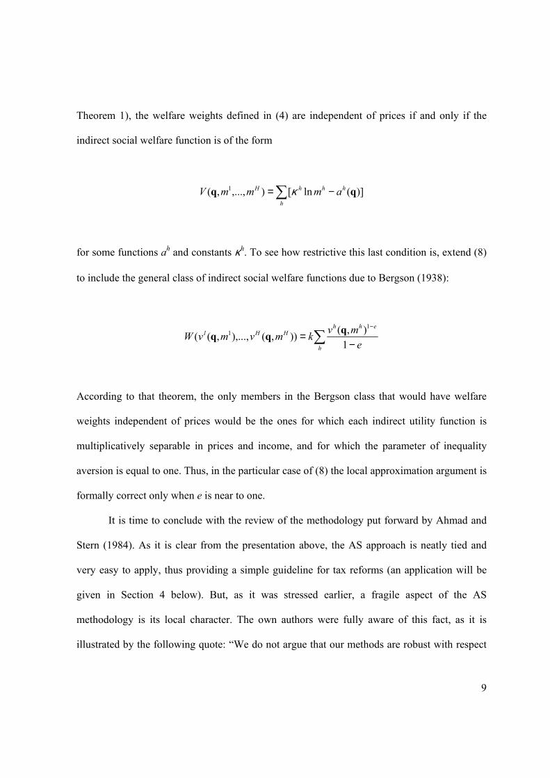
Theorem 1), the welfare weights defined in (4) are independent of prices if and only if the

indirect social welfare function is of the form

∑ −=h

hhhH ammmV )](ln[),...,,( 1 qq κ

for some functions ah and constants κh. To see how restrictive this last condition is, extend (8)

to include the general class of indirect social welfare functions due to Bergson (1938):

∑ −=

−

h

ehhHH1

emvkmvmvW

1),()),(),...,,((

11 qqq

According to that theorem, the only members in the Bergson class that would have welfare

weights independent of prices would be the ones for which each indirect utility function is

multiplicatively separable in prices and income, and for which the parameter of inequality

aversion is equal to one. Thus, in the particular case of (8) the local approximation argument is

formally correct only when e is near to one.

It is time to conclude with the review of the methodology put forward by Ahmad and

Stern (1984). As it is clear from the presentation above, the AS approach is neatly tied and

very easy to apply, thus providing a simple guideline for tax reforms (an application will be

given in Section 4 below). But, as it was stressed earlier, a fragile aspect of the AS

methodology is its local character. The own authors were fully aware of this fact, as it is

illustrated by the following quote: “We do not argue that our methods are robust with respect

10

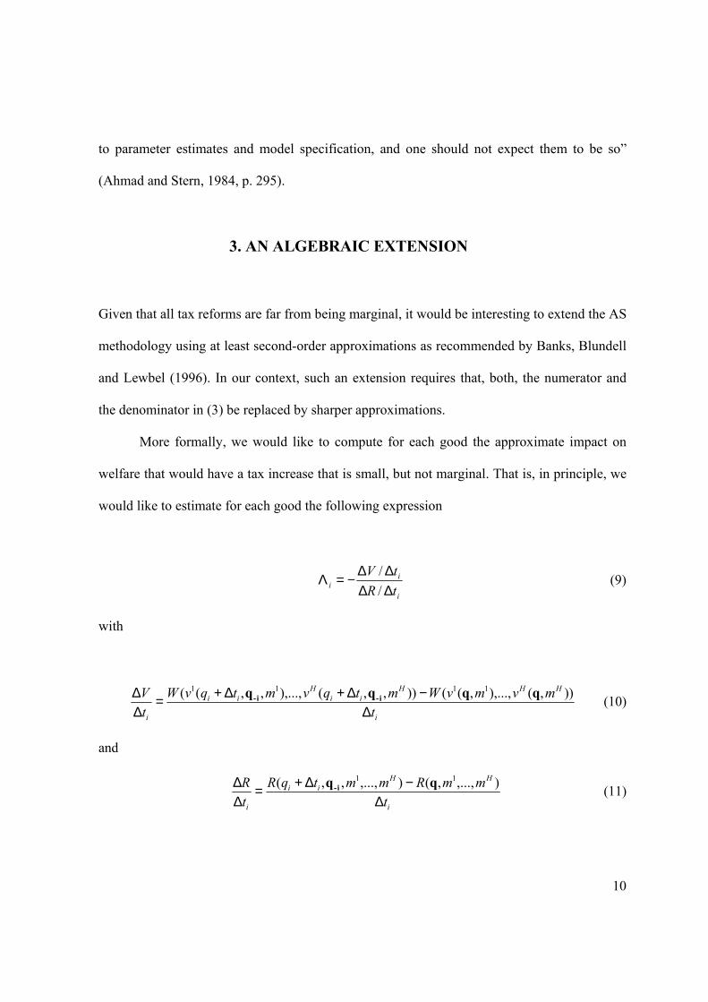
to parameter estimates and model specification, and one should not expect them to be so”

(Ahmad and Stern, 1984, p. 295).

3. AN ALGEBRAIC EXTENSION

Given that all tax reforms are far from being marginal, it would be interesting to extend the AS

methodology using at least second-order approximations as recommended by Banks, Blundell

and Lewbel (1996). In our context, such an extension requires that, both, the numerator and

the denominator in (3) be replaced by sharper approximations.

More formally, we would like to compute for each good the approximate impact on

welfare that would have a tax increase that is small, but not marginal. That is, in principle, we

would like to estimate for each good the following expression

i

ii tR

tV∆∆∆∆−=Λ

// (9)

with

i

HHHii

Hii

i tmvmvWmtqvmtqvW

tV

∆−∆+∆+=

∆∆ )),(),...,,(()),,(),...,,,(( 1111 qqqq i-i- (10)

and

i

HHii

i tmmRmmtqR

tR

∆−∆+=

∆∆ ),...,,(),...,,,( 11 qq i- (11)

11

and where, as usual, by q-i is meant the vector that includes all the elements of q except for the i-

th component.

The second-order Taylor expansion of (10) is given by

2

2

2 i

i

ii tVt

tV

tV

∂∂∆+

∂∂≈

∆∆

so that

( ) hi

hii

h

i

i

h

h

i

xqt

tV

+∆+−≈

∆∆ ∑ εεβ β2

1 (12)

where, for each household h, the first elasticity inside the parentheses refers to the price

elasticity of the welfare weight, while the second one refers to the own-price elasticity of

individual demand. Likewise, the second-order Taylor expansion of (11) gives

∑

∂∂+−∆++

∆+≈∆∆

kk

i

kiikiki

i

iki

i

kkiii

i

i

i

Xt

qqt

qqX

qt

tR εεεετε )1(

21 (13)

Thus, after simplifying (12) and (13), the following variant to the Ahmad-Stern

approach is suggested in this paper: To analyze, for each of the goods, the approximate impact

on social welfare that would have a tax increase that is small, but not necessarily marginal,

instead of the first-order approximation given in equation (7) above, use the following second-

order approximation:

12

( )

∑

∑

−∆++

∆+

+∆+

=Λ

kkkkiki

i

ikiiii

i

i

hii

hii

h

i

i

h

h

i

XqqtXq

qt

xqqt

εετε

εεβ β

)1(2

11

21

(14)

Note that the numerator on the right-hand side of equation (14) contains the price

elasticity of each welfare weight, so that the measure suggested in this paper requires, in

general, the estimation of the full demand system. This result is not surprising. Indeed, it

seems even natural once one takes into account the main message given by Banks et al.

(1996).

If, at the risk of losing theoretical soundness and numerical precision, one wants to

simplify (14) to allow for a comparison with the AS approach, one can continue using as a local

approximation the Atkinson social indirect utility function given in (8). In such a case, the

implied welfare weights will be independent of prices, and (14) can be approximated as:

∑

∑

−∆++

∆+

∆+≈Λ

kkkkiki

i

ikiiii

i

i

hii

hii

i

i

h

h

i

XqqtXq

qt

xqqt

εετε

εβ

)1(2

11

21

(15)

Note that aside from the fact that (15) is more realistic than (7), insofar as it allows for

non-marginal tax changes, both equations are similar in terms of their informational

requirements. The only difference is that now (15) requires estimates of the own-price

elasticities of household demands (all the terms of the form hiiε ), which would seem to be a

13

daunting task. Although it is unlikely to have that information even when the full demand

system is estimated (given the lack of this type of panel data in most countries), one could use

instead the average demand responses in each income decile, as it is done in the next section.

Furthermore; if one does not count with that information either, then one could use as a proxy

the own-price elasticity of aggregate demand.

4. AN APPLICATION TO MEXICO USING BOTH APPROACHES

Regarding the Mexican economy, Urzúa (1994 and 2001) provided the first studies that

attempted to estimate the welfare consequences of several indirect tax reforms enacted by the

Mexican Congress in the nineties. Following the work by King (1983), those papers relied on

the estimation of full-demand systems and were based on the income and expenditure surveys

made by the government in 1989 and 1994, respectively. The Almost Ideal Demand System

(AIDS) of Deaton and Muellbauer (1980) was used in both papers, after taking care of the fact

that expenditures could be zero for some goods, and after making use, in the case of Urzúa

(2001), of the generalized method of moments to allow for a more flexible demand system.

More recently, Campos (2002), in his Master’s thesis, has also followed King’s

approach to analyze the social impact of several potential tax reforms that have been discussed

in the political arena over the last few years. Although the main purpose of his thesis is only

tangentially related to our purposes, we can still make use of some of his estimates of

consumption levels and elasticities to provide an example of how to use the AS methodology

and its variant.

14

The demand system estimated by Campos is termed the Quadratic Almost Ideal

Demand System (QUAIDS), and is due to Banks, Blundell and Lewbel (1997). It nests the

AIDS system, although it also allows for quadratic Engel curves, a feature that seems to match

observed expenditure patterns of individual consumers and households.

More precisely, assume that the budget share spent on good i by any household is of the

form

ii

ijij

n

1=jii u

am

damq + = w +

+

+∑

2

)(ln

)()(lnln

qqqθ

δγα

where ui is normally distributed with zero mean and variance 2σ , and where

q q + q + = a jiij

n

j=1

n

=1iii

n

=1i0 lnln

21ln)(ln γαα ∑∑∑q

and

∏=

=n

ii

iqd1

)( δq

We have to impose, as usual, three conditions on the parameters to make the model given above

a bona fide demand system: adding-up, homogeneity, and symmetry. The expressions for those

constraints can be found in Banks, Blundell and Lewbel (1997), but for our purposes it is of

more interest to present here expressions for the QUAIDS model elasticities. As shown by,

15

those authors, the uncompensated price elasticities, the ones that are required in the AS

approach and its variant presented in earlier sections, are given by

iji

ijij w

δµ

ε −=

where the Kronecker delta δij equals one when i = j and zero otherwise, and where

2

)(ln

)(ln

)(ln

)(2

−

+

+−= ∑ qqqq a

md

qa

md

ji

kkjkj

iiijij

δθγαθδγµ

Campos estimated the model by three-step nonlinear least squares, using as data set the

income and expenditure survey of 10,108 households made by the government in the year 2000

(INEGI, 2001). The author aggregated the consumption goods reported in that survey to obtain

just five composite goods, using as the composition criterion the differential treatment accorded

by Mexican tax laws to the value added tax. The implied prices were calculated as the weighted

mean of the prices involved, using as weights the relative expenditures. A brief description of

those five composite goods is given in the first two columns of Table 1 below.

The other five columns in that table present the uncompensated cross-price elasticities

that were obtained by that author (all of them statistically significant). Although there is no need

to reproduce here the income elasticities implied by the model, it may be of interest to note that

Campos found that the first three composite goods were necessities; namely, non-processed

16

Table 1

Composite Goods and Uncompensated Cross-Price Elasticities*

Composite goods 1 2 3 4 5

Good 1: Non-processed food and dairy products -0.636 0.033 0.013 0.260 0.152

Good 2: Processed food, clothing and appliances -0.026 -0.672 0.012 -0.027 -0.041

Good 3: Alcoholic beverages and tobacco -0.062 0.038 -0.816 0.295 2.140

Good 4: Medicines -0.255 -0.608 0.022 -1.032 -0.185

Good 5: Education -0.106 -0.289 -0.031 -0.218 -0.955

* Source: Campos (2002, tables 3 and 5).

17

food; processed food, clothing and appliances; and alcoholic beverages and tobacco. On the

other hand, medicines and education were found to be luxuries.

Using Table 1, we are now ready to illustrate the AS approach and the variant suggested

in this paper. It is important to remember, as noted in the last section, that in order to allow for a

direct comparison between both approaches we will make use here of Atkinson’s function, given

in equation (8) above, since the AS approach assumes that the indirect social welfare function is

independent of prices. Thus, although our variant not only allows but even calls for the use of

indirect functions dependent on prices, such as the general Bergsonian family cited earlier, here

we will sacrifice theoretical soundness for the sake of comparison. But it almost goes without

saying that, because of the use of (15) instead of (14), we should expect that the numerical

differences resulting from (15) and (7) will be minor.

Regarding the tax changes to be considered here, the attention will be centered on the

value-added tax (VAT), although a similar exercise could be made in the case of other excise

taxes (such as the so-called IEPS on tobacco and alcoholic beverages). As a first step, it should

be noted that in Mexico the VAT rate for the case of non-processed food, medicines and

education is currently equal to zero, while the VAT rate for processed food (as well as for

clothing and appliances) and for alcoholic beverages (including tobacco) is equal to 15%. It

should also be noted that in our model tk is by construction a quantity tax (i.e., a tax per unit of

consumption of good k), not an ad-valorem tax. Thus, given a VAT rate of 15%, the

corresponding τk (the proportion of the tax on good k relative to the consumer price) equals

13%.

Making use now of the elasticities given in Table 1, as well as of raw data on prices,

consumption levels and aggregate demand responses, all of them classified by deciles, Table 2

18

presents the marginal social cost of raising an extra revenue by increasing the tax on each

composite good, using the expression for each λi given in (7). The results are given for four

different levels of inequality aversion: from e=0, when there is no aversion whatsoever, to e=3,

when the welfare of the poorest has a substantial relative weight in the social welfare function. It

is usually argued that e should oscillate between one and two, and so the corresponding results

for those two values are also reported.

As can be seen from Table 2, when there is no inequality aversion the preferred good to

be taxed is the one composed by alcoholic beverages and tobacco. But once the parameter is

increased the preferred choice becomes education. Therefore, as the concern about the poorest

takes more importance, one has to shift from “sin taxes” to taxes on education.

This last result should be interpreted with extreme care, however, since in this type of

models education is wrongly put on the same footing as mere consumption. That is, the model

does not take into consideration the fact that the social return on education is certainly larger

than the private return. For instance, the spillovers from education may arise from positive

externalities across workers and/or endogenous skill-based technical change (see, respectively,

Lucas, 1988, and Acemoglu and Angrist, 2000).

Table 2 also presents the results obtained when we use second-order approximations to

compute each Λi in (15), after assuming a uniform increase of $2 in the quantity taxes for all

goods (that magnitude was chosen since it represented an increase from 0% to about 10% in the

case of the average price of good 1). The price change was taken to be the same across goods to

make a fair comparison with the results obtained using (7), but, of course, one of the advantages

of (15) over (7) is that now the goods could be accorded a differential tax treatment!

19

Table 2

Marginal and Approximate Social Welfare Costs

Degree of inequality aversionMarginal and approximate social cost

e=0 e=1 e=2 e=3

Non-processed food and dairy productsλ1 1.018 0.125 0.051 0.040Λ1 1.062 0.129 0.053 0.041

Processed food, clothing and appliancesλ2 1.096 0.055 0.008 0.004Λ2 1.088 0.054 0.008 0.004

Alcoholic beverages and tobaccoλ3 0.869 0.098 0.044 0.036Λ3 0.851 0.096 0.043 0.035

Medicinesλ4 1.022 0.059 0.011 0.006Λ4 0.988 0.057 0.010 0.006

Educationλ5 1.021 0.035 0.004 0.001Λ5 0.992 0.034 0.003 0.001

20

It should be noted that even though both variants suggest the same optimal way to raise

revenue, the ranking of the social costs is not always the same for both methods. Consider, for

instance, the two different rankings that are given in Table 2 for the case of composite goods 1

and 2 (whether or not this difference is statistically significant would be very hard to verify,

though, given the complex functional forms of both lambdas).

Before closing this section, it may be interesting to address here what is known in the

literature on optimal taxation as the “inverse optimum” problem. In our context, this problem

could be encapsulated in the following question: If we were to assume that the actual tax

structure is optimal, what is the implied degree of inequality aversion in Mexico?

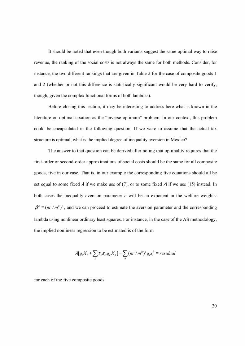
The answer to that question can be derived after noting that optimality requires that the

first-order or second-order approximations of social costs should be the same for all composite

goods, five in our case. That is, in our example the corresponding five equations should all be

set equal to some fixed λ if we make use of (7), or to some fixed Λ if we use (15) instead. In

both cases the inequality aversion parameter e will be an exponent in the welfare weights:

ehh mm )/( 1=β , and we can proceed to estimate the aversion parameter and the corresponding

lambda using nonlinear ordinary least squares. For instance, in the case of the AS methodology,

the implied nonlinear regression to be estimated is of the form

residualxqmmXqXqh

hii

eh

kkkkikii =−+ ∑∑ )/(][ 1ετλ

for each of the five composite goods.

21

The corresponding estimates obtained in that fashion are very similar in both cases: λ =

0.717 and e = 0.125 if we use equation (7), and Λ = 0.721 and e = 0.121 if we use equation (15).

These results have to be interpreted with care since there are only five observations, and,

furthermore, the corresponding t-statistics are not significant in either case. Yet, if are willing

to jump to a conclusion with such a few observations, the moral to be drawn is worrisome: the

implied inequality aversion is quite low in the case of Mexico. To put it in another way, the

indirect tax system in Mexico is everything but progressive.

5. CONCLUSIONS

This paper has presented a variant to the marginal tax analysis first put forward by Ahmad and

Stern two decades ago. The variant, as given in equation (14), recognizes that welfare weights

do depend on prices, and that tax reforms involve more than marginal changes and include

differential treatments across goods. The paper also presented an example based on the

Mexican tax system, after simplifying (14) to (15) to allow for a fair comparison with the AS

approach (which implicitly, and wrongly, assumes that the indirect social welfare function

does not depend on prices).

As a final remark, we should note that the approach suggested here should be used only

as a preliminary analysis that can shed some light on optimal tax changes across goods. After

such directions are identified, then the analysis should be complemented with a systemic one

of the type proposed by King (1983), which makes use of equivalent incomes to make global

welfare comparisons among different tax regimes.

22

REFERENCES

Acemoglu, D. and J. Angrist (2000), “How Large are Human Capital Externalities? Evidence from Compulsory Schooling Laws”, NBER Macro Annual 2000, pp. 9-59. Ahmad, E. and N. Stern (1984), “The Theory of Reform and Indian Indirect Taxes”, Journal of Public Economics, 25, pp. 259-98. Ahmad, E. and N. Stern (1991), The Theory and Practice of Tax Reform in Developing Countries, Cambridge: Cambridge University Press. Atkinson, A. B. (1970), “On the Measurement of Inequality”, Journal of Economic Theory, 2, pp. 244-263. Banks, J., R. Blundell and A. Lewbel (1996), “Tax Reform and Welfare Measurement: Do We Need Demand System Estimation?”, Economic Journal, 106, pp. 1227-1241. Banks J., R. Blundell and A. Lewbel (1997), “Quadratic Engel Curves and Consumer Demand”, Review of Economics and Statistics, 79, pp. 527-539. Bergson, A. (1938), “A Reformulation of Certain Aspects of Welfare Economics”, Quarterly Journal of Economics, 52, pp. 310-334. Campos, R. M. (2002), Impacto de una reforma fiscal en México. Una estimación con base en sistemas de demanda, Master’s thesis, Centro de Estudios Económicos, El Colegio de México. Cragg, M. (1991), “Do We Care? A Study of Canada’s Indirect Tax System”, Canadian Journal of Economics, 24, pp. 121-143. Decoster, A. and E. Schokkaert (1990), “Tax Reform Results with Different Demand Systems”, Journal of Public Economics, 41, pp. 277-296. Deaton, A. and J. Muellbauer (1980), “An Almost Ideal Demand System”, American Economic Review, 70, 312-326. Diamond, P. and J. A. Mirlees (1971), “Optimal Taxation and Public Production”, I and II, American Economic Review, 61, pp. 8-27 and 261-278. INEGI (2001), ENIGH-2000: Encuesta Nacional de Ingresos y Gastos de los Hogares, Aguascalientes, México: INEGI.

23

Kaiser, H. and P. B. Spahn (1989), “On the Efficiency and Distributive Justice of Consumption Taxes: A Study on VAT in West Germany”, Zeitschrift fur Nationalokonomie, 49, pp. 199-218. King, M. A. (1983), “Welfare Analysis of Tax Reforms Using Household Data”, Journal of Public Economics, 21, pp. 183-214. Lucas, R. E. (1988), “On the Mechanics of Economic Development”, Journal of Monetary Economics, 22, pp. 3-42. Madden, D. (1995), “An Analysis of Indirect Tax Reform in Ireland in the 1980’s”, Fiscal Studies, 16, pp. 18-37. Urzúa, C. M. (1994), “An Empirical Analysis of Indirect Tax Reforms in Mexico”, unpublished manuscript presented at the XIII Latin American Meeting of the Econometric Society held in Caracas, Venezuela. Urzúa, C. M. (2001), “Welfare Consequences of a Recent Tax Reform in Mexico”, Estudios Económicos, 16, pp. 57-72.