the accounting review pp. 501–538 an evaluation of...

501

THE ACCOUNTING REVIEWVol. 80, No. 22005pp. 501–538

An Evaluation of Accounting-BasedMeasures of Expected Returns

Peter D. EastonUniversity of Notre Dame

Steven J. MonahanINSEAD, Accounting and Control Area

ABSTRACT: We develop an empirical method that allows us to evaluate the reliabilityof an expected return proxy via its association with realized returns even if realizedreturns are biased and noisy measures of expected returns. We use our approach toexamine seven accounting-based proxies that are imputed from prices and contem-poraneous analysts’ earnings forecasts. Our results suggest that, for the entire cross-section of firms, these proxies are unreliable. None of them has a positive associationwith realized returns, even after controlling for the bias and noise in realized returnsattributable to contemporaneous information surprises. Moreover, the simplest proxy,which is based on the least reasonable assumptions, contains no more measurementerror than the remaining proxies. These results remain even after we attempt to purgethe proxies of their measurement error via the use of instrumental variables and group-ing. We provide additional evidence, however, that demonstrates that some proxies arereliable when the consensus long-term growth forecasts are low and/or when analysts’forecast accuracy is high.

Keywords: cost of capital; expected rate of return; earnings forecasts; residual incomevaluation; measurement error.

I. INTRODUCTION

We develop an empirical approach for evaluating the reliability of estimates of theexpected rate of return on equity capital. We use our approach to examine sevenaccounting-based proxies that are imputed from prices and contemporaneous

Workshop participants at the American Accounting Association Annual Meetings, Columbia University, FloridaState University, Hong Kong University of Science and Technology, INSEAD, Texas A&M University, TheUniversity of Alabama, The University of Arizona, University of Chicago, University of Houston, The Univer-sity of Iowa, University of Notre Dame, and University of Rochester provided valuable comments on an earlierdraft. We thank Ray Ball, Phil Berger, Bruce Johnson, Doron Nissim, Lubos Pastor, Marlene Plumlee, ShivaSivaramakrishnan, Jim Wahlen, and two anonymous referees for helpful comments and suggestions. Earningsforecast data are from I /B/E /S.

Editor’s note: This paper was accepted by Terry Shevlin, Senior Editor.Submitted October 2003

Accepted September 2004

502 Easton and Monahan

The Accounting Review, April 2005

analysts’ earnings forecasts.1 We show that for the entire cross-section of firms, none ofthese proxies has a positive association with realized returns after controlling for changesin expectations about future cash flows and future discount rates. Moreover, a naı̈ve measureof expected return (the inverse of price to forward earnings) contains no more, and oftenless, measurement error than the remaining proxies. We provide additional evidence, how-ever, that demonstrates that some proxies are reliable when the consensus long-term growthforecasts are low and/or when analysts’ forecast accuracy is high.

Similar to the majority of studies in the empirical asset-pricing literature, our inferencesabout the reliability of a particular expected return proxy are based on its association withrealized returns. However, unlike these studies, we assume that realized returns are biasedand noisy measures of expected returns. This assumption is motivated by evidence presentedin Elton (1999) and Fama and French (2002). These authors demonstrate that ‘‘informationsurprises,’’ which cause realized returns to differ from expected returns, do not cancel outover time or across firms.2 We show that these information surprises are also correlatedwith expected returns. Taken together, these observations imply that simple regressions ofrealized returns on expected return proxies yield spurious inferences because of omittedcorrelated variables bias.

In light of the above, we adopt an approach that explicitly takes into account the biasand noise in realized returns. Our approach is based on the linear return decompositiondeveloped by Vuolteenaho (2002), who demonstrates that information surprises equal thechange in expectations about future cash flows (i.e., cash flow news) less the change inexpectations about future discount rates (i.e., return news). Hence, he provides a theoreticalfoundation for a regression of realized returns on proxies for expected returns, cash flownews, and return news. The coefficients from this regression serve as our initial source ofevidence about the reliability of the expected return proxies.

A problem with basing our inferences on the regression coefficients discussed aboveis that the estimates of these coefficients are affected by errors in variables bias. Becausewe cannot observe expectations and changes in expectations, all of the regressors (i.e., theexpected return proxy, the cash flow news proxy, and the return news proxy) are measuredwith error. The sign and magnitude of the bias attributable to measurement error is generallyunknown when more than one variable in a multivariate regression contains measurementerror (e.g., Rao 1973). However, the return decomposition demonstrates that if the com-ponents of realized returns are measured without error, then the estimates of the slopecoefficients in a regression of realized returns on expected returns, cash flow news, andreturn news are unambiguously equal to 1. Thus, the bias in the coefficients correspondingto our empirical proxies is well defined. This, in turn, implies that we can modify theeconometric method described in Garber and Klepper (1980) and Barth (1991) to develop

1 Examples of studies that use accounting-based expected return proxies to evaluate the cross-sectional determi-nants of expected returns include: Chen et al. (2004), Dhaliwal et al. (2003), Gebhardt et al. (2001), Francis etal. (2003), Gode and Mohanram (2003), Hail (2002), Hail and Leuz (2004), Hribar and Jenkins (2004), and Leeet al. (2003). We illustrate our method by examining variants of several of the expected return proxies used inthese studies. However, our method can be used to evaluate any expected return proxy including those basedon forecasts of dividends and prices (e.g., Botosan 1997; Botosan and Plumlee 2002; Brav et al. 2004; Franciset al. 2004).

2 Elton (1999, 1199) states: ‘‘The use of average realized returns as a proxy for expected returns relies on a beliefthat information surprises tend to cancel out over the period of a study and realized returns are therefore anunbiased measure of expected returns. However, I believe there is ample evidence that this belief is misplaced.’’Fama and French (2002) provide evidence that suggests the abnormally large equity premium observed duringthe post-war era was attributable to information surprises that took the form of consistent downward revisionsin expected future discount rates. We elaborate on these issues in Section II.

An Evaluation of Accounting-Based Measures of Expected Returns 503


rankings of measurement error variances of the expected return proxies that serve as oursecond source of evidence about their reliability.

Our empirical results suggest that, for the entire cross-section of firms, the accountingbased proxies we evaluate are not reliable estimates of the expected rate of return on equitycapital. None of the proxies has a positive association with realized returns even after wecontrol for changes in expectations about future cash flows and future discount rates. More-over, the measurement error variance of a naı̈ve proxy based on the price-to-forward-earnings ratio is never greater, and often lower, than the error variances of the remainingproxies. These results are robust. For example, we evaluate the effectiveness of two com-monly used methods for mitigating measurement error: instrumental variables, and group-ing. Neither of these approaches lead to improvements in the associations between theexpected return proxies and realized returns, nor do they affect the ordering of the mea-surement error variances (i.e., the measurement error variance of the naı̈ve proxy is nodifferent from the error variances of the remaining proxies).

Further analyses, however, demonstrate that certain proxies are reliable for some subsetsof the data. First, we show that the reliability of the proxies is decreasing in the magnitudeof consensus long-term earnings growth rate, and that an analog of the measure of expectedreturns used by Claus and Thomas (2001) is a reliable proxy for a subsample of firms withlow consensus long-term growth forecasts. We also demonstrate that when ex post analysts’forecasts errors are low, all of the proxies have a positive association with expected returns.Combining these two sets of results with the fact that ex post forecast errors are increasingin analysts’ long-term growth forecasts leads us to draw two conclusions: (1) the lack ofreliability for the general cross-section is partially attributable to low-quality analysts’ fore-casts, and (2) the consensus long-term earnings growth rate is a useful ex ante indicator ofreliability (the higher the forecasted growth, rate the lower the reliability).

We contribute to the accounting and finance literatures in three ways. First, we developan empirical approach for drawing unbiased inferences about an expected return proxyfrom its association with realized returns even if realized returns are biased and noisy.Second, we provide evidence suggesting that in most circumstances the expected returnproxies we evaluate are unreliable. This implies that there is a need for further research onthe development of accounting-based measures of expected returns, and that extant evidencebased on the proxies we evaluate should be interpreted with caution. Finally, we provideevidence consistent with the notion that the apparent lack of reliability of our expectedreturn proxies is partially attributable to the quality of analysts’ earnings forecasts, whichsuggests that further study of the determinants of analysts’ forecast errors is warranted.3

Two other studies explicitly aimed at evaluating the reliability of accounting-basedmeasures of expected returns are Botosan and Plumlee (2005) and Guay et al. (2003).Botosan and Plumlee (2005) rank measures of expected returns by comparing coefficientsfrom regressions of expected return proxies on assumed risk factors (e.g., CAPM beta,equity market value, leverage, etc.). While this approach has intuitive appeal, it requiresthat the researcher make the implicit assumption that the risk factors evaluated are correctand exhaustive, which is unlikely. As discussed in Section II, the return decomposition thatserves as the foundation for our tests is based on a tautology: that is, our analyses are based

3 Like other studies (e.g., Abarbanell and Bushee 1997; Francis et al. 2000) that document large valuation errorswhen analysts’ forecasts are used in valuation, we are unable to distinguish between two possible explanationsfor the measurement error in the expected return proxies: (1) errors in the forecasts, and (2) the restrictiveassumptions underlying the implementations of the valuation models used to obtain the estimates of the expectedrate of return.



on a fully specified model of the relation between an expected return proxy and trueexpected return.

The approach adopted by Guay et al. (2003) is similar to ours as they also evaluatethe relation between various expected return proxies and realized returns. There is a crucialdifference between our study and theirs, however; we include cash flow news and returnnews proxies in our regressions, whereas they do not. In particular, the evidence presentedin Guay et al. (2003) is based on simple regressions of realized return on the expectedreturn proxy. Hence, as discussed above, the associations they document are likely to bebiased measures of the relation between the expected return proxies and true expectedreturn. In Section IV, we provide evidence that bias of this nature exists and is non-trivial.

The remainder of the paper unfolds in the following manner. In the next two sectionswe describe our empirical method, discuss our proxies of interest, and describe our sample.Our main empirical results are presented in Section IV. The results of our instrumentalvariables analyses, grouping analyses, and analyses of the relation between the reliabilityof the expected return proxies and analyst long-term growth forecasts are discussed inSection V. We provide concluding comments in Section VI.

II. EMPIRICAL METHODWe begin by describing Vuolteenaho’s (2002) linear decomposition of realized return

into three components: expected return, cash flow news, and return news. Vuolteenaho’s(2002) decomposition forms the basis of a linear regression of realized return on the proxiesfor its components. After discussing this regression we describe how measurement error inthe regressors leads to bias in the regression coefficients. Finally, we describe the mannerin which we refine the method discussed in Garber and Klepper (1980) and Barth (1991)so that we can isolate the portion of the coefficient bias that is solely attributable to themeasurement error in the expected return proxy.

The Components of Realized ReturnsVuolteenaho (2002) demonstrates that firm i’s realized, continuously compounded re-

turn for year t�1, , can be decomposed into three components: (1) expected return,rit�1

, (2) changes in expectations about future cash flows (cash flow news, ), and (3)er cnit�1 it�1

changes in expectations about future discount rates (return news, ). In particular:rnit�1

r � er � cn � rn . (1)it�1 it�1 it�1 it�1

In Equation (1) expectations underlying are formed at the end of year t, whereaserit�1

and reflect revisions in expectations occurring during year t�1.4 A detailedcn rnit�1 it�1

description of Vuolteenaho’s (2002) return decomposition, which is similar to the well-known return decomposition developed by Campbell (1991), is provided in Appendix A.Empirical proxies for expected return, , cash flow news, , and return news,er cnit�1 it�1

, are described in Section III.rnit�1

Three observations about Equation (1) warrant mentioning. First, Equation (1) is de-rived from a tautology; hence, our analyses do not rely on implicit or explicit assumptionsabout investor rationality, the nature of market equilibrium, transactions costs, etc. Second,the linear return decompositions developed by Campbell (1991) and Vuolteenaho (2002)

4 In Equation (1) the negative sign on return news, , reflects the fact that, ceteris paribus, increases in futurernit�1

discount rates lead to a decrease in contemporaneous price and, thus, realized return, , is lower than expectedrit�1

return, .erit�1



are well accepted. For example, a number of studies in finance use variations of Equation(1) as a means of evaluating the determinants of realized returns (comprehensive literaturereviews can be found in Campbell et al. [1997, Chapter 7] and Cochrane [2001, Chapter20]). Finally, since Equation (1) reflects the effect of changes in expectations about futurecash flows and future discount rates on realized returns, it provides a direct means of dealingwith Elton’s (1999) argument that information surprises cause realized returns to be a biasedand noisy measure of expected returns.

The third point is especially pertinent to our study. Bias in realized returns implies thatthe estimate of the slope coefficient taken from a simple regression of realized returns onexpected returns is also biased. If changes in expectations about future cash flows (discountrates) are associated with contemporaneous expected returns, the coefficient on expectedreturns will be affected by correlated omitted variables bias. This is quite plausible. Forexample, an explanation for the equity premium puzzle is that during the post-war periodthe U.S. (and other Western nations) experienced an unprecedented run of ‘‘good luck.’’5

Hence, the expected future rate of return required by investors as compensation for holdingthe market portfolio steadily declined (i.e., economy-wide rnit�1 was negative), which, perEquation (1), caused the realized equity premium to be consistently larger than expected.6

This, in turn, led to higher than expected realized returns on individual stocks. Moreover,the magnitude of the bias at the individual stock level was arguably increasing in thecovariance between a stock’s return and the return on the market portfolio. It follows thatchanges in expectations about future discount rates (i.e., ) were correlated with bothrnit�1

realized and expected returns (i.e., and ), and the coefficient on is biased ifr er erit�1 it�1 it�1

is omitted from the regression.7rnit�1

The Regression Based on Vuolteenaho’s (2002) Return DecompositionWe begin our analyses by estimating the following regression for each expected return

proxy:

r � � � � � er̂ � � � cn̂ � � � rn̂ � ε . (2)it�1 0t�1 1t�1 it�1 2t�1 it�1 3t�1 it�1 it�1

In Equation (2) , , and represent the expected return proxy, the cash flower̂ cn̂ rn̂it�1 it�1 it�1

news proxy, and the proxy for negative return news (i.e., �1 � , which we refer torn )it�1

as the return news proxy. The expected return proxies, the cash flow news proxies, and thereturn news proxies are described in Section III. If these empirical proxies are measuredwithout error, , , and are equal to 1 and is equal to 0. Hence, one means� � � �1t�1 2t�1 3t�1 0t�1

of evaluating a particular measure of expected returns is to conduct a test of the differencebetween and 1. Unfortunately, these tests do not lead to clear-cut inferences; because�1t�1

we are unable to observe expectations or revisions in expectations, each of the regressorsin Equation (2) contains error, which implies the bias in a particular regression coefficientis a complex function of the measurement errors in all of the regressors (e.g., Rao 1973).To circumvent this problem we use a refinement of the approach discussed in Garber and

5 See Cochrane (2001, Chapter 21, 460–462) for a discussion of the equity premium puzzle. The discussion underthe heading ‘‘Luck and a Lower Target’’ is particularly relevant.

6 Fama and French (2002) provide specific evidence of this phenomenon.7 A similar argument can be made for the inclusion of in the regression. In particular, if changes incnit�1

expectations about future cash flows are correlated with investment opportunities, which, in turn, are correlatedwith expected returns, will be correlated with both realized and expected return. Berk et al. (1999) developcnit�1

a model in which firms’ optimal investment choices are associated with expected returns.



Klepper (1980) and Barth (1991) to isolate the portion of the bias in that is solely�1t�1

attributable to the measurement error in .er̂it�1

Measurement Error AnalysisIn this subsection we describe the intuition underlying the method we use to isolate

the portion of the bias in that is solely attributable to measurement error in .� er̂1t�1 it�1

Appendix B contains a rigorous description of our econometric approach, which is centeredon the following regression:

A A A� � � � � � ε � � � ε � � � ε � � . (3)Cit�1 0t�1 1t�1 1it�1 2t�1 2it�1 3t�1 3it�1 it�1

In Equation (3) equals the difference between firm i’s observed, realized return for�Cit�1

year t�1, and the sum of the empirical measures of its components (i.e., �� rCit�1 it�1

� � � ); thus, equals the combined measurement error in ourer̂ cn̂ rn̂ �it�1 it�1 it�1 Cit�1

empirical proxies. Each regressor (i.e., , and ) essentially equals the adjustedA A Aε , ε ε1it�1 2it�1 3it�1

error from a regression of one of the proxies on the remaining two (e.g., is obtainedAε1it�1

by regressing on and ). Hence, each regression coefficient in Equation (3)er̂ cn̂ rn̂it�1 it�1 it�1

measures the relation between the error in a particular proxy and the combined error in allthe proxies. The expression for the regression coefficient corresponding to , which weAε1it�1

refer to as the ‘‘noise variable,’’ is:8

2� � � (� ) � {�(� , � ) � �(� , � )} � {�(er , � )1t�1 1it�1 1it�1 2it�1 1it�1 3it�1 it�1 2it�1

� �(er , � )}. (4)it�1 3it�1

In Equation (4) �2 ) is the variance of the measurement error in the expected return(�1it�1

proxy, ) denotes the covariance between the measurement error in and�(� , � er̂1it�1 2it�1 it�1

the measurement error in , �( ) is the covariance between the measurementcn̂ � , �it�1 1it�1 3it�1

error in and the measurement error in , �( ) is the covariance betweener̂ rn̂ er , �it�1 it�1 it�1 2it�1

true expected return and the measurement error in , and �( ) is the covari-cn̂ er , �it�1 it�1 3it�1

ance between true expected return and the measurement error in . If the covariancern̂it�1

terms are constant across expected return proxies, then variation across proxies in the noisevariable is solely attributable to variation in the measurement error in the expected returnproxies (i.e., �2 . This implies that the expected return proxy with the smallest noise(� ))1it�1

variable contains the least measurement error and is the most reliable. Hence, we begin ourmeasurement error analyses by estimating Equation (3) for each of the expected returnproxies of interest.

A problem with using the noise variables to rank our expected return proxies is that itis unlikely that the covariance terms shown in Equation (4) are constant across expectedreturn proxies. Because each of our measures of the expected rate of return is based on aunique set of assumptions about dividends, future earnings growth, and terminal profita-bility, it is likely that the relation between the error in each proxy and the errors in theremaining independent variables is also unique. This implies that inferences based on therelative magnitudes of the different estimates of the noise variable may not provide a

8 As shown in Appendix B, the expressions for and are similar to the expressions for . Given that� � �2t�1 3t�1 1t�1

our primary interest relates to the measurement error in the expected return proxies, we choose to focus thediscussion in the body of the paper on .�1t�1



meaningful basis for inferring the relative magnitudes of ). To circumvent this prob-2� (�1it�1

lem we refine the econometric approach developed by Garber and Klepper (1980) and Barth(1991) and estimate ‘‘modified noise variables:’’9

M 2� � � (� ) � {�(er , cn ) � �(er , rn )}1t�1 1it�1 it�1 it�1 it�1 it�1

� {�(� , cn ) � �(� , rn )}. (5)1it�1 it�1 1it�1 it�1

In Equation (5) �( � ) equals the covariance between true ex-er , cn ) �(er , rnit�1 it�1 it�1 it�1

pected return and the sum of true cash flow news and true return news.Two observations regarding the modified noise variables are pertinent. First, while there

is reason to believe � ) is not equal to zero, it involves only�(er , cn ) �(er , rnit�1 it�1 it�1 it�1

the true values of the constructs, which implies it is constant across proxies. Hence, ifdifferences in � ) are second order, which is a reasonable�(� , cn ) �(� , rn1it�1 it�1 1it�1 it�1

assumption, differences in the modified noise variables are primarily attributable to differ-ences in the measurement error variances of the proxies (i.e., �2 )).10 Second, isM(� �1it�1 1t�1

not a function of the measurement errors in the cash flow news and return news proxies(i.e., and ). This implies that rankings based on are unaffected by risk-M� � �1it�1 2it�1 1r�1

related measurement errors in and .cn̂ rn̂it�1 it�1

SummaryTo summarize, bias and noise attributable to information surprises imply that simple

regressions of realized returns on expected return proxies yield spurious inferences that areattributable to omitted correlated variables. Hence, we include measures of cash flow newsand return news in our regressions (i.e., Equation (2)). However, because all of the regres-sors in Equation (2) contain measurement error, the regression coefficient corresponding tothe expected return proxy is not a clear-cut indicator of the reliability of this proxy. Toovercome this problem we use a refinement of the method described in Garber and Klepper(1980) and Barth (1991) to estimate the measurement error variances.

III. EMPIRICAL PROXIES AND SAMPLE CONSTRUCTIONAccounting-Based Measures of Expected Return

In this section we provide a brief overview of the seven expected return proxies weevaluate, each of which is imputed from prices and contemporaneous earnings forecasts.Our first proxy is based on the assumption that expected cum-dividend aggregate earningsfor the next two years are valuation sufficient. Hence, it essentially equals the inverse ofthe price-to-forward-earnings ratio. For this reason we refer to it as rpe. The purpose ofincluding rpe in our analyses is to provide a naı̈ve benchmark (based on restrictive as-sumptions about future earnings growth).11

Our next four expected return proxies are each derived from the finite-horizon versionof the earnings, earnings growth model developed by Ohlson and Juettner-Nauroth (2003)and described in Easton (2004):

9 The refinements are described in Appendix B.10 Two observations support the assumption that differences in � ) across expected�(� , cn ) �(� , rn1it�1 it�1 1it�1 it�1

return proxies are second order: (1) there is no reason to believe errors in our ability to measure expectationsat time t are correlated with revisions in true expectations occurring during time t�1, and (2) even if thiscorrelation is non-zero, there is no reason to believe its magnitude differs across proxies.

11 To be precise, the valuation model underlying rpe relies on the assumption that after year t�2 cum-dividendaggregate earnings grow at a rate equal to the cost of capital.



eps eps � r � dps � (1 � r) � epsit�1 it�2 it�1 it�1P � �it r r � (r � �agr)

eps agrit�1 it�1� � . (6)r r � (r � �agr)

In Equation (6) Pit is price at the end of year t, epsit�� is the year t forecast of year t��earnings per share, dpsit�1 is the year t forecast of dividends paid in year t�1, r is theexpected rate of return, and �agr is a growth rate. Following Easton (2004), we refer tothe difference between expected year-two cum-dividend accounting earnings (i.e., epsit�2

� r � dpsit�1) and normal accounting earnings that would be expected given earnings ofperiod one (i.e., (1 � r) � epsit�1) as ‘‘abnormal growth in earnings’’ or agrit�1. Hence,�agr equals the perpetual rate of change in abnormal growth in earnings beyond the forecasthorizon.

The first proxy derived from Equation (6) embeds the assumption that no dividendsare paid in year t�1 and that �agr equals 0. As shown in Easton (2004), this proxy isequal to the square root of the inverse of the PEG ratio; hence, we refer to it as rpeg.

12

Relaxing the assumption that dpsit�1 is equal to 0 yields a modified version of the PEGratio and a proxy we refer to as rmpeg.

13 A criticism of rpeg and rmpeg is that the assumptionof constant abnormal growth in earnings is too restrictive. Gode and Mohanram (2003)avoid this criticism by assuming �agr is a cross-sectional constant equal to the differencebetween the risk-free rate of interest and 3 percent. We refer to their proxy as rgm. Easton(2004), on the other hand, simultaneously estimates r and �agr for portfolios of stocksallowing for cross-sectional variation in �agr. We refer to his proxy as r�agr.

14

Our final two measures of expected return are derived from the residual income valu-ation model. We refer to the first of these two proxies as rct because it is based on the workof Claus and Thomas (2001). Claus and Thomas (2001) assume that earnings grow at theanalysts’ consensus long-term growth rate until year t�5. They assume earnings after yeart�5 grow at the rate of inflation, which is set equal the risk-free rate less 3 percent. Thesecond proxy derived from the residual income model is based on the work of Gebhardtet al. (2001); hence, we refer to it as rgls. Gebhardt et al. (2001) use actual earnings forecaststo develop estimates of return on equity for year t�1 and t�2. They assume that accountingreturn on equity linearly fades to the historical industry median between years t�3 andt�12, and remains constant thereafter.15

Finally, note that all of our expected return proxies reflect continuous compounding.In particular, the value of for a particular set of assumptions equals ln(1 � r), whereer̂it�1

r is the discount rate implied by the corresponding valuation model. The valuation modelsunderlying each of the expected return proxies and details of their calculation are providedin Table 1.

12 The PEG ratio, which is equal to the PE ratio divided by the short-term earnings growth rate, is a commonmeans of comparing stocks in analysts’ reports.

13 Since I /B /E /S does not provide forecasts of dividends, we assume dpst�1 equals dpst (i.e., dividends per sharepaid in year t).

14 This method simultaneously estimates the expected rate of return and the growth rate for a portfolio of firmsthat have similar PEG ratios. Assigning these estimates of the expected rate of return to each firm in the portfoliointroduces measurement error. However, it allows us to avoid having to make ad hoc assumptions about �agr.

15 While both rct and rgls are based on the residual income valuation model, as discussed above, each reflectsdifferent assumptions about the manner in which ROE evolves after year t�2. Our empirical results demonstratethat these differences in assumptions lead to significant differences in the statistical properties of the two proxies.For example, as shown in Table 3, the correlation between rct and rgls is less than 0.50.

An

Evaluation

ofA

ccounting-Based

Measures

ofE

xpectedR

eturns509

The

Accounting

Review

,A

pril2005

TABLE 1Summary of Empirical Proxies, Data Sources, and Sample Construction

er̂it�1

Expected Return ProxiesValuation Model Comments

rpe Pit �eps � r � dps � epsit�1 it it�2

2(1 � r) � 1

rpeg eps � epsit�2 it�1P �it 2r

rmpeg eps � r � dps � epsit�2 it it�1P �it 2r

rgm eps eps � r � dps � (1 � r) � epsit�1 it�2 it it�1P � �it r r � (r � �agr)�agr is the contemporaneous yield on a ten-year government bond less 3

percent.

r�agr eps eps � r � dps � (1 � r) � epsit�1 it�2 it it�1P � �it r r � (r � �agr)r and �agr are estimated simultaneously via the approach discussed in Easton

(2004).

rct4 (ROE � r) � bpsit�� it��1P � bps � �it it �(1 � r)��1

(ROE � r) � bps � (1 � �)it�5 it�4� 4(r � �) � (1 � r)

� (1 � ltgi)��2 ∀ � � 2. ltgi is theROE � eps /bps . eps � epsit�� it�� it��1 it�� it�2

I /B/E/S consensus forecast of the growth rate in earnings per share. bpsit��

� bpsit��1 � epsit�� (1 � K). For profitable firms K � max(0,min(dpsit /epsit,1)). For loss firms K � max(0,min(dpsit / (.06 � bpsit),1)). � is thecontemporaneous yield on a ten-year government bond less 3 percent. Wesolve for r via an iterative procedure.

rgls11 (ROE � r) � bpsit�� it��1P � bps � �it it �(1 � r)��1

(ROE � r) � bpsit�12 it�11� 11r � (1 � r)

ROEit�� epsit�� /bpsit��1 for � � 1,2. ROEit�� ROEit��1 � fade ∀ � � 2.fade � (ROEit�2 � HIROEt) /10, HIROEt is the historical industry medianROE for all firm-years in the same industry spanning year t�4 through yeart with positive earnings and equity book values. We use the industrydefinitions shown in Fama and French (1997). bpsit�� bpsit��1

� (1 � ROEit�� K). For profitable firms K � max(0,min(dpsit /epsit,1)).For loss firms K � max(0,min(dpsit / (.06 � bpsit), 1)). We solve for r via aniterative procedure.

(continued on next page)

510E

astonand

Monahan

The

Accounting

Review

,A

pril2005

TABLE 1 (continued)

Cash Flow News Proxy, , and Return News Proxy,cn̂ rn̂it�1 it�1

Formula Comments

cn̂ � (roe � froe ) � ( froe � froe )it�1 it it,t it�1,t�1 it,t�1

� � ( froe � froe )it�1,it�2 it,t�21 � � t

roeit � ln(1�ROEit), ROEit � epsit /bpsit�1. froeij,k � ln(1�ROEij,k), ROEij,k

denotes the forecast of return on equity for fiscal year k and is based on theconsensus I /B/E/S forecast made at the end of year j. The approach weuse to estimate is discussed in Appendix A. t is estimated on an annualbasis via the pooled, cross-sectional regression shown in Equation (9).

rn̂ � � (er̂ � er̂ )it�1 it�2 it�11 �

varies across expected return proxies. The approach we use to estimate rn̂it�1

is discussed in Appendix A. When conducting our multivariate analyses wedefine return news as:

rn̂ � � � (er̂ � er̂ )it�1 it�2 it�11 �

We use continuously compounded returns; hence, the value of for a particular proxy is equal to the natural log of 1 plus the discount rate imputed from theer̂it�1

valuation model underlying that proxy. Pit is the closing share price for fiscal year t per Compustat (data item 199), dpsit is dividends per share for year t perCompustat (data item 26), and bpsit (bpsit�1) is equity book value at the end of year t (t�1) per Compustat (data item 60) divided by common shares outstanding at theend of year t (t�1) per Compustat (data item 25). epsit is reported earnings per share for year t per I /B /E /S. epsit�1 is the consensus earnings per share forecast foryear t�1 per I /B /E /S. When available, we use the actual, consensus forecast for year t�2 as our proxy for epsit�2. When actual forecasts are unavailable we useI /B /E /S forecasts of growth in earnings as the basis for developing our proxy for epsit�2. We eliminate firm-years occurring before 1981 and after 1998, or that do nothave a December fiscal year-end. We delete firm-years with missing or non-positive Pit, bpsit, bpsit�1, or common shares outstanding; with negative epsit�1; withepsit�2 � epsit�1; with ltgi � 0; with missing cum-dividend, continuously compounded stock return in year t�1 per CRSP, rit�1; with a missing cash flow news proxy,

; or a missing return news proxy, . Finally, firm-years with values of or in the top or bottom 1/2 percentile of the annual,cn̂ rn̂ r , er̂ , cn̂ rn̂it�1 it1 it�1 it�1 it�1 it�1

cross-sectional distribution are considered outliers and deleted. Our final sample consists of 15,680 firm-years.



Cash Flow News and Return News ProxiesIn the Vuolteenaho (2002) return decomposition (Equation (1)), cash flow news cnit�1

is the component of realized returns corresponding to the change in investors’ expectationsabout future cash flows. As shown in Appendix A, cash flow news is defined as follows:

��1cn � �E � roe . (7)�� it�1 t�1 it��

��1

In Equation (7) �Et�1[.] equals Et�1[.] � Et[.], is a number slightly less than 1, and roeis the natural log of 1 plus the accounting rate of return on equity. This equation impliesthat a revision in expectations about future profitability leads to a realized return that islarger (in magnitude) than expected return. The effect on realized return of a particularrevision in expectations about future profitability is not, however, a cross-sectional constant.Rather, the size of the effect depends on investors beliefs about growth, which are capturedby . In particular, as shown in Appendix A, is monotonically increasing in the price-to-dividend ratio, which is generally considered a function of future growth opportunities.16

Hence, can be viewed as a ‘‘capitalization factor.’’We use the following formula to estimate our cash flow news proxies:

cn̂ � (roe � froe ) � ( froe � froe )it�1 it it,t it�1,t�1 it,t�1

� � ( froe � froe ). (8)it�1,t�2 it,t�21 � � t

In Equation (8) froeij,k denotes forecasted roe for fiscal year k and is based on the consensusforecast of epsik made in December of year j, t is the expected persistence of roe as oftime t.17 The manner in which we estimate , which varies with the price-to-dividend ratio,is discussed in Appendix A. Our cash flow news proxy embeds the assumption that roefollows a first order autoregressive process after year t�1. This assumption is consistentwith evidence presented in Beaver (1970), Freeman et al. (1982), and Sloan (1996).

We estimate t via the following pooled cross-sectional and time-series regression:

roe � � � roe . (9)i��1 0t t i�

In Equation (9) � is a number between t and t�9 and the sample includes all firm-years inthe same Fama and French (1997) industry with requisite data in year t�9 through year t(i.e., for each year t we estimate t using firm years between year t�9 and year t). Giventhat accounting methods, competition, and risk vary across industry, our use of an industryspecific t reduces the potential for bias attributable to risk-related measurement error in

.cn̂it�1

16 Consider the dividend growth model ⇒ � which clearly implies the price-to-dividenddps P 1

P � ,r � g dps r � g

ratio is increasing in the growth rate, g.17 We include (roeit � froeit,t) in Equation (8) to capture the change in expectations that occurs in year t�1 upon

the announcement of actual year t earnings. As discussed below, is based on information that becomesfroeit,t

publicly available on the third Thursday of the last fiscal month of year t.



In the Vuolteenaho (2002) return decomposition (Equation (1)), return news rnit�1 isthe component of realized returns corresponding to the change in investors’ expectationsabout future discount rates.18 As shown in Appendix A, return news is defined as follows:

��1rn � �E � r . (10)�� it�1 t�1 it��

��2

has the same role in the above expression as its role in cnit�1 (i.e., it is a capitalizationfactor that allows the sensitivity of realized return to a given change in the expected discountrate to vary across stocks on the basis of variation in growth). We use the following formulato estimate our return news proxy:

rn̂ � � (er̂ � er̂ ). (11)it�1 it�2 it�11 �

That is, varies across valuation models, and embeds the assumption that changes inrn̂it�1

the discount rate are permanent (i.e., the discount rate follows a random walk). This as-sumption is consistent with the fact that each of our expected return proxies is the geometricaverage of all expected future discount rates.

Our cash flow and return news proxies are a function of analysts’ forecasts, which alsoserve as the basis of our expected return proxies. This is unavoidable as expectations andchanges in expectations are inextricably linked. For example, the expected return assignedto a particular stock is a function of the risk of the expected payoffs; hence, reflectscnit�1

revisions in the expectations underlying . Similar logic implies that ander rn erit�1 it�1 it�1

are related, which, in turn, implies varies across valuation models.rn̂it�1

Sample ConstructionPrice at fiscal year-end, equity book value, dividends, and number of shares outstanding

are obtained from the 1999 Compustat annual primary, secondary, tertiary, and full coverageresearch files. Earnings forecasts are derived from the summary 2000 I/B/E/S tape. Wedetermine median forecasts from the available analysts’ forecasts on the I/B/E/S file thatis released on the third Thursday of December. We delete firms with non-December fiscalyear-ends so that the market-implied discount rate and growth rate are estimated at thesame point in time for each firm-year observation.19 For observations in 1995, for example,the December forecasts became available on the 21st day of the month. These data includedforecasts for a fiscal year ending ten days later (i.e., December 31, 1995) and either anearnings forecast for each of the fiscal years ending December 31, 1996 and 1997 (i.e.,

18 In the context of a multifactor asset-pricing model, return news is attributable to an unforeseen change in therisk-free rate, unforeseen changes in the factor loadings (i.e., the ‘‘betas’’), and unforeseen changes in the factorpremiums (e.g., the market risk premium). In the instant case, a change in the risk-free rate is irrelevant becauseit has an equal effect on all equities; hence, it has no effect on the cross-sectional distribution of realized returns.Changes in factor loadings are relevant to the extent they vary across stocks. These changes occur because ofchanges in the correlation between a particular factor and stock returns, or a change in the volatility of thefactor. Changes in factor premiums affect a particular equity by an amount proportionate to the correspondingfactor loading for that stock. Hence, even though these changes are economy-wide, they do affect the cross-sectional distribution of realized returns. Changes in factor premiums occur because of changes in investors’appetite for risk, ability to diversify, etc.

19 While limiting our sample to firms with fiscal-years that end in December reduces the power of our tests, it isunlikely that it leads to bias; hence, our inferences are likely unaffected by this research design choice.



epsit�1 and epsit�2) or the forecast for the fiscal year ending December 31, 1996 (i.e., epsit�1)and a forecast of growth in earnings per share for the subsequent years. When available,we use the actual forecasts for the subsequent year (in this example, 1997) as our proxyfor epsit�2. When actual forecasts are unavailable we use I/B/E/S forecasts of growth inearnings as the basis for developing our proxy for epsit�2. Realized returns for the yearfollowing the earnings forecast date (in the example, January 1, 1996 to December 31,1996) are obtained from the Center for Research in Security Prices (CRSP) Monthly Returnfile.

We eliminate firm-year observations (1) prior to 1981 and after 1998 because there arevery few observations with complete data in these years, (2) with missing price, dividendsper share, or common shares outstanding, (3) with missing or negative book value of equity,(4) with negative , (5) with � , (6) with a negative consensus forecasteps eps epsit�1 it�2 it�1

of long-term earnings per share growth, (7) with missing cum-dividend, continuously com-pounded stock return in year t�1, (8) with a missing cash flow news proxy, or (9) with amissing return news proxy. Finally, firm-years with values of , , or inr er̂ , cn̂ rn̂it�1 it�1 it�1 it�1

the top or bottom 1/2 percentile of each yearly, cross-sectional distribution are consideredoutliers and deleted. Our final sample consists of 15,680 firm-year observations.

IV. MAIN EMPIRICAL RESULTSIn this section we discuss the descriptive statistics, correlations, and the results of our

main empirical tests. As discussed above and in Appendix B, the Vuolteenaho (2002) returndecomposition pertains to continuously compounded returns; hence, we transform realizedreturns and each of the measures of expected return by taking the log of 1 plus the proxyof interest. Analyses of untransformed values lead to similar inferences. Descriptive statis-tics and correlations are based on the definition of shown in Equation (11). The valuern̂it�1

of underlying our multivariate tests is obtained from Equation (11) and is equal to:rn̂it�1

� � (er̂ � er̂ ).it�2 it�11 �

Descriptive StatisticsDescriptive statistics for realized returns, the expected return proxies, and the cash flow

news proxy are shown on Panel A of Table 2. The median estimate of rpe is 8.3 percent,which is considerably less than the median realized return of 12.2 percent. Moreover, asshown in the column titled less rf , 31 percent of the firm-years in our sample have valuesof rpe below the contemporaneous value of the continuously compounded risk-free rate.These results suggest that rpe is a downward-biased measure of expected return. However,they do not provide evidence about the cross-sectional association between rpe and trueexpected returns, which is the pertinent issue given our research question.20

20 Given the expected risk premium on a stock is rarely less than zero, a high value of less rf suggests that theaverage of the expected return proxy is a poor measure of mean expected returns. However, less rf is notinformative about the cross-sectional characteristics of the proxy (i.e., bias does not imply noise). Hence, in thecontext of our research question a high value of less rf is not prima facie evidence that an expected returnproxy is unreliable. Conversely, our empirical tests relate to the cross-sectional characteristics of the expectedreturn proxies and do not shed light on whether the proxies are useful measures of mean expected returns. Forexample, while our evidence suggests that variation in rct does not capture variation in true expected returns,we cannot conclude that the evidence presented in Claus and Thomas (2001) regarding the magnitude of theexpected equity premium is unreliable.



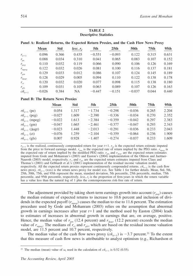
TABLE 2Descriptive Statistics

Panel A: Realized Returns, the Expected Return Proxies, and the Cash Flow News Proxy

Mean Std less rf 5th 25th 50th 75th 95th

rit�1 0.096 0.366 0.435 �0.551 �0.093 0.122 0.315 0.631rpe 0.088 0.034 0.310 0.041 0.065 0.083 0.107 0.152rpeg 0.110 0.032 0.119 0.066 0.090 0.106 0.126 0.169rmpeg 0.122 0.032 0.026 0.081 0.100 0.116 0.137 0.181rgm 0.129 0.033 0.012 0.086 0.107 0.124 0.145 0.189r�agr 0.128 0.029 0.005 0.094 0.110 0.122 0.138 0.178rct 0.120 0.032 0.020 0.077 0.098 0.115 0.138 0.180rgls 0.109 0.031 0.105 0.063 0.089 0.107 0.126 0.163cn̂it�1 �0.026 0.384 NA �0.447 �0.151 �0.037 0.044 0.440

Panel B: The Return News Proxies

Mean Std 5th 25th 50th 75th 95th

(pe)rn̂it�1 0.054 1.317 �1.734 �0.298 �0.036 0.265 2.204(peg)rn̂it�1 �0.027 1.609 �2.390 �0.336 �0.034 0.270 2.352(mpeg)rn̂it�1 �0.022 1.613 �2.384 �0.359 �0.042 0.297 2.383(gm)rn̂it�1 �0.047 1.665 �2.461 �0.377 �0.047 0.293 2.343(�agr)rn̂it�1 �0.023 1.448 �2.013 �0.291 �0.036 0.233 2.043(ct)rn̂it�1 �0.076 1.259 �2.104 �0.359 �0.064 0.236 1.909(gls)rn̂it�1 0.007 0.928 �1.407 �0.274 �0.037 0.233 1.609

rit�1 is the realized, continuously compounded return for year t�1. rpe is the expected return estimate imputedfrom the price to forward earnings model. rpeg is the expected rate of return implied by the PEG ratio. rmpeg isthe expected rate of return implied by the modified PEG ratio. rgm and r�agr are the expected return estimatesimputed from Gode and Mohanram’s (2003) and Easton’s (2004) implementation of the Ohlson and Juettner-Nauroth (2003) model, respectively. rct and rgls are the expected return estimates imputed from Claus andThomas’s (2001) and Gebhardt et al.’s (2001) implementation of the residual income valuation model,respectively. All the expected return proxies represent continuously compounded returns. is the cash flowcn̂it�1

news proxy. (xxx) is the return news proxy for model xxx. See Table 1 for further details. Mean, Std, 5th,rn̂it�1

25th, 50th, 75th, and 95th represent the mean, standard deviation, 5th percentile, 25th percentile, median, 75thpercentile, and 95th percentile, respectively. less rf is the proportion of firm-years in which the return variablehas a value less than the natural log of 1 plus the contemporaneous risk-free rate of return.

The adjustment provided by taking short-term earnings growth into account (rpeg) causesthe median estimate of expected returns to increase to 10.6 percent and inclusion of divi-dends in the expected payoff (rmpeg) causes the median to rise to 11.6 percent. The estimationprocedure used by Gode and Mohanram (2003) relies on the assumption that abnormalgrowth in earnings increases after year t�1 and the method used by Easton (2004) leadsto estimates of increases in abnormal growth in earnings that are, on average, positive.Hence, the median value of rgm (12.4 percent) and r�agr (12.2 percent) exceeds the medianvalue of rmpeg. The medians of rct and rgls, which are based on the residual income valuationmodel, are 11.5 percent and 10.7 percent, respectively.

The median value of the cash flow news proxy ( ) is �3.7 percent.21 To the extentcn̂it�1

that this measure of cash flow news is attributable to analyst optimism (e.g., Richardson et

21 The median (mean) value of t used in the calculation of is 0.52 (0.55).cn̂it�1



al. 2001) that is ignored by the market, the negative median value of cash flow newsrepresents measurement error in our cash flow news proxies. Moreover, given that ourexpected return proxies and return news proxies are also derived from analysts’ forecasts,the negative median value of cash flow news implies that these constructs are also measuredwith error.

Descriptive statistics for our return news proxies are shown in Panel B of Table 2.Since these estimates equal the change in the estimate of expected return over the realizedreturn interval, they differ across the various estimates of expected returns. The medianestimates of return news are consistently negative. For example, the median return newsimplied by the change in rpeg is �3.4 percent and the median return news for rct is �6.4percent. In light of the fact that prices rose during our sample period, the decline in ourexpected return proxies suggests a coincident decline in the equity premium.

CorrelationsTable 3, Panel A summarizes the correlations among realized returns, the expected

return proxies, and the estimates of cash flow news. Pearson product moment (Spearmanrank order) correlations are shown above (below) the diagonal. Correlations between ourreturn news proxies and the remaining variables of interest are shown in Panel B. Thecorrelations are the temporal averages of the annual cross-sectional correlations. Thet-statistics are the ratio of these averages to their temporal standard errors. We focus ourdiscussion on the Spearman correlations. The Pearson correlations lead to similarinferences.

There is a significant positive correlation between realized return and two of the ex-pected return proxies: rct (0.073, t-statistic of 2.35) and rgls (0.061, t-statistic of 1.95). Noneof the correlations between the remaining expected return proxies and realized returns isstatistically different from zero at the 0.05 level. Moreover, three of the correlations arenegative. These negative correlations imply that the cash flow news and return news com-ponents of realized returns reflect more than random measurement error, which only causesattenuation bias and has no affect the sign of the correlation.22 Rather, these correlationssupport the arguments we made in Section II. Specifically, true cash flow news and truereturn news are correlated with our expected return proxies. Hence, in order to avoid draw-ing spurious inferences attributable to omitted correlated variables bias it is crucial that wecontrol for variation in cash flow news and returns news.

As expected, the correlation between realized returns and the estimate of cash flownews is positive and significant (Spearman correlation of 0.314 with a t-statistic of 16.99).The significant negative correlation between the cash flow news proxy and rpe and thesignificant negative correlations between the cash flow news proxy and each of the estimatesof expected returns derived from the abnormal growth in earnings model (i.e., Equation(6)) provide additional support for our argument that including a cash flow news proxy inour regressions is necessary in order to avoid correlated omitted variables bias. Thesenegative correlations suggest that firms with relatively high discount rates experienced larger

22 The correlation between realized return ( � � � ) and an expected return proxyr er cn rn er̂it�1 it�1 it�1 it�1 it�1

equals . If cash flow news and return news are simply random mea-�(er , er̂ ) � �(cn � rn , er̂ )it�1 it�1 it�1 it�1 it�1

�(r ) � �(er̂ )it�1 it�1

surement error, then the second term in the numerator equals zero and the sign is equal to the sign of the firstterm. The sign of the first term is positive unless the covariance between true expected return and the measure-ment error in the expected return proxy is negative and has an absolute value greater than the variance of trueexpected returns. This is unlikely.


TABLE 3Correlations among Key Variables

Panel A: Realized Returns, the Expected Return Proxies, and the Cash Flow News Proxy

rit�1 rpe rpeg rmpeg rgm r�agr rct rgls cn̂it�1

rit�1 0.048 �0.032 0.013 �0.006 �0.010 0.050 0.057 0.243(1.16) (�1.40) (0.54) (�0.34) (�0.52) (1.68) (2.03) (13.71)

rpe 0.056 0.384 0.537 0.339 0.325 0.713 0.599 �0.039(1.31) (18.98) (15.73) (14.93) (17.56) (38.29) (33.13) (�2.77)

rpeg �0.028 0.386 0.892 0.880 0.866 0.591 0.415 �0.141(�1.13) (19.48) (44.39) (37.33) (26.11) (33.64) (23.05) (�12.44)

rmpeg 0.023 0.577 0.860 0.956 0.817 0.664 0.394 �0.132(0.85) (18.41) (38.84) (60.30) (20.10) (39.26) (19.52) (�12.94)

rgm �0.003 0.351 0.843 0.936 0.811 0.567 0.278 �0.134(�0.13) (13.87) (31.81) (47.21) (18.89) (30.02) (11.25) (�13.31)

r�agr 0.015 0.360 0.910 0.807 0.795 0.498 0.331 �0.129(�0.68) (19.89) (101.45) (38.93) (32.16) (20.54) (14.84) (�11.89)

rct 0.073 0.713 0.620 0.724 0.610 0.573 0.428 �0.088(2.35) (40.22) (37.09) (59.88) (28.21) (38.55) (14.13) (�4.55)

rgls 0.061 0.605 0.471 0.451 0.317 0.418 0.470 0.148(1.95) (38.42) (28.48) (25.16) (12.12) (24.07) (17.86) (4.11)

cn̂it�1 0.314 �0.030 �0.222 �0.178 �0.191 �0.210 �0.113 0.068(16.99) (�1.98) (�20.03) (�14.93) (�13.53) (�19.73) (�6.16) (3.43)

Panel B: Correlations among Return News Proxies, Realized Returns, the Expected ReturnProxies, and the Cash Flow News Proxy

ModelPearson Product Moment

rit�1 er̂it�1 cn̂it�1

Spearman Rank Orderrit�1 er̂it�1 cn̂it�1

(pe)rn̂it�1 �0.339 �0.245 0.055 �0.429 �0.291 0.125(�8.97) (�7.79) (2.89) (�14.74) (�6.49) (4.81)

(peg)rn̂it�1 �0.174 �0.338 0.031 �0.200 �0.375 0.123(�5.36) (�10.77) (1.77) (�7.17) (�12.00) (4.49)

(mpeg)rn̂it�1 �0.198 �0.343 0.026 �0.264 �0.387 0.090(�6.36) (�15.79) (1.48) (�10.55) (�18.10) (3.84)

(gm)rn̂it�1 �0.153 �0.356 0.018 �0.214 �0.402 0.075(�5.29) (�14.91) (1.10) (�9.17) (�17.71) (3.69)

(�agr)rn̂it�1 �0.164 �0.414 0.018 �0.174 �0.434 0.097(�5.92) (�11.64) (1.01) (�7.38) (�16.39) (4.17)

(ct)rn̂it�1 �0.134 �0.286 0.126 �0.223 �0.323 0.251(�3.63) (�11.44) (8.21) (�6.58) (�10.27) (10.22)

(gls)rn̂it�1 �0.444 �0.240 0.024 �0.475 �0.272 �0.001(�12.52) (�9.09) (1.44) (�17.03) (�7.55) (�0.03)

All correlations reflect averages of the annual correlations. t-statistics (in parentheses) equal the ratio of thecorrelation to its temporal standard error. Cells above (below) the diagonal of the correlation matrix shown inPanel A correspond to Pearson product moment (Spearman rank order) correlations. The rows in Panel B are thecorrelations between the measure of return news for a particular model and realized returns, expected returns asmeasured via the model of interest, and the cash flow news proxy. is the realized, continuously compoundedrit�1

return for year t�1. rpe is the expected return estimate imputed from the price to forward earnings model. rpeg isthe expected rate of return implied by the PEG ratio. rmpeg is the expected rate of return implied by the modifiedPEG ratio. rgm and r�agr are the expected return estimates imputed from Gode and Mohanram’s (2003) andEaston’s (2004) implementation of the Ohlson and Juettner-Nauroth (2003) model, respectively. rct and rgls arethe expected return estimates imputed from Claus and Thomas’s (2001) and Gebhardt et al.’s (2001)implementation of the residual income valuation model, respectively. All the expected return proxies representcontinuously compounded returns. is the cash flow news proxy. (xxx) is the return news proxy forcn̂ rn̂it�1 it�1

model xxx.See Table 1 for further details.



than average negative information surprises about future cash flows during the time periodunder study.23

The correlation between rgls and the cash flow news proxy is positive and significant,however (Spearman correlation of 0.068 with a t-statistic of 3.43). A rationale for thisphenomenon is as follows. There are two essential differences between rgls and the remain-ing expected return proxies: (1) the residual income valuation model is anchored on year tequity book value, and (2) the terminal value correction used by Gebhardt et al. (2001) isa function of historical industry median return on equity (ROE). Thus, compared to theremaining estimates of expected returns, the amount of cross-sectional variation in rgls

attributable to variation in the firm-specific book-to-market ratio and variation in industryROE is relatively high. These facts are a likely explanation for the positive correlationbetween rgls and the estimate of cash flow news: variation in our cash flow news proxy isalso a function of variation in equity book value and it is possible that analysts tend torevise their optimistic forecasts of ROE toward the industry ROE.24

Table 3, Panel B summarizes the Pearson and Spearman correlations among our returnnews proxies and realized return, the cash flow news proxy, and the corresponding estimatesof expected return. As expected, the correlation between each of the estimates of returnnews and realized returns are significantly less than zero (all the t-statistics are less than�3.5). The correlations between the return news proxies and the corresponding proxies forexpected returns are all negative and statistically significant. These results are consistentwith a decline in the equity premium during our sample period. As discussed in SectionII, if the equity premium fell during the sample period, then stocks with high betas (and,thus, high expected returns) experienced larger than average downward revisions in ex-pected future discount rates (i.e., ).25 Hence, in order to avoid drawing spurious in-rnit�1

ferences attributable to omitted variables bias, it is crucial we include a proxy for returnnews in our regressions.

Multivariate AnalysesResults pertaining to our multivariate tests are shown in Tables 4 and 5. The regression

coefficients shown in these tables are the temporal averages of the regression coefficientsobtained from annual cross-sectional regressions. The t-statistics are computed via the ap-proach described in Fama and MacBeth (1973).

Summary statistics from the estimation of the regression of realized returns on theempirical measures of its components (expected return, cash flow news, and return news)—Equation (2)—are presented in Table 4 for each of the expected return proxies. The esti-mates of the coefficient �1 on the expected return proxies are negative for each of theregressions except the regression based on rct, and this estimate is not statistically differentfrom zero. Moreover, untabulated results demonstrate that all of the estimates of �1 are

23 These correlations are also consistent with the notion that analysts’ forecasts are too extreme in the sense thathigh forecasts are too high and low forecasts are too low. For example, if year zero analysts’ forecasts are toohigh (too low), the implied discount rate will be biased upward (downward) and analysts’ forecast errors andrevisions will be negative (positive).

24 We test this conjecture by estimating annual regressions of each expected return proxy on the contemporaneousbook-to-market ratio and historical industry ROE. The average, untabulated R2s from these regressions are: rpe

0.135, rpeg 0.027, rmpeg 0.045, rgm 0.029, r�agr 0.026, rct 0.05, and rgls 0.225. These results support our conjecturefor two reasons: (1) the highest average R2 is obtained in the regression involving rgls, and (2) the averageR2 is higher when the correlation between the expected return proxy and the cash flow news proxy is higher.

25 Alternatively, these negative correlations may be attributable to measurement error in our proxies. For example,a decline in analyst optimism may have occurred during our sample period, or extremely high (low) forecastsmay be followed by larger than average downward (upward) revisions.



TABLE 4Multivariate Analyses for Annual Portfolios

Regression: r � � � � � er̂ � � � cn̂ � � � rn̂ � εit�1 0t�1 1t�1 it�1 2t�1 it�1 3t�1 it�1 it�1

er̂it�1 �0 �1 �2 �3 R2

rpe 0.16 �0.54 0.29 0.10 0.22(5.33) (�1.46) (5.28) (10.36)

rpeg 0.19 �0.67 0.26 0.04 0.12(6.26) (�2.81) (5.59) (6.43)

rmpeg 0.15 �0.36 0.27 0.05 0.13(4.02) (�1.20) (5.67) (7.11)

rgm 0.16 �0.40 0.26 0.04 0.11(4.90) (�1.75) (5.67) (5.98)

r�agr 0.20 �0.70 0.26 0.04 0.11(6.16) (�2.70) (5.70) (6.41)

rct 0.09 0.10 0.30 0.05 0.13(1.98) (0.25) (5.09) (4.29)

rgls 0.24 �1.15 0.29 0.19 0.30(7.91) (�4.21) (5.52) (13.52)

Separate regressions are estimated for each of the 18 annual cross-sections of data. Parameter estimates equal theaverage of the annual regression coefficients. t-statistics (in parentheses) equal the ratio of the parameterestimates to their temporal standard errors. R2 is the mean R2 from the annual regressions. er̂ , cn̂ , rn̂ ,it�1 it�1 it�1

and represent the expected return proxy, the cash flow news proxy, the return news proxy and the realized,rit�1

continuously compounded return for year t�1. rpe is the expected return estimate imputed from the price toforward earnings model. rpeg is the expected rate of return implied by the PEG ratio. rmpeg is the expected rate ofreturn implied by the modified PEG ratio. rgm and r�agr are the expected return estimates imputed from Gode andMohanram’s (2003) and Easton’s (2004) implementation of the Ohlson and Juettner-Nauroth (2003) model,respectively. rct and rgls are the expected return estimates imputed from Claus and Thomas’s (2001) and Gebhardtet al.’s (2001) implementation of the residual income valuation model, respectively. All the expected returnproxies represent continuously compounded returns.See Table 1 for further details.

significantly less than 1 at the 0.01 level. These results suggest there is a considerableamount of measurement error in each of the expected return proxies. On the other hand,as discussed in Section II and Appendix B, the observed bias in �1 may be attributable toother factors; hence, the need for additional analyses. As expected, the estimates of thecoefficients on and are significantly positive. For example, for the regressioncn̂ rn̂it�1 it�1

based on rgls, the estimate of the coefficient on is 0.29 (t-statistic of 5.52) and thecn̂it�1

estimate of the coefficient on is 0.19 (t-statistic of 13.52). Nonetheless, untabulatedrn̂it�1

results demonstrate that these estimates are also significantly less than one, which impliesthat these constructs are also measured with error.

The results of estimating Equation (3) for each of our return proxies are shown in Table5. Before proceeding with a discussion of the regression coefficients it is interesting to notethat Equation (3) explains a considerable portion of the cross-sectional variation in the



TABLE 5Multivariate Analyses for Annual Portfolios

A A ARegressions: � � � � � � ε � � � ε � � � ε � �Cit�1 0t�1 1t�1 1it�1 2t�1 2it�1 3t�1 3it�1 it�1

M M A A A� � � � � � ε � � � ε � � � ε � �Cit�1 0t�1 1t�1 1it�1 2it�1 2it�1 3t�1 3it�1 it�1

Model

Unmodified Noise Variables(�Cit�1 is the regressand)

�0 �1 �2 �3 R2

Modified Noise Variablesis the regressand)M(�Cit�1

�0M�1 �2 �3 R2

pe 0.161 0.0076 0.132 1.214 0.94 0.161 0.0005 0.132 1.214 0.94(5.33) (9.42) (3.65) (6.36) (5.33) (1.42) (3.65) (6.36)

peg 0.189 0.0152 0.136 2.098 0.96 0.189 0.0012 0.136 2.098 0.96(6.26) (7.70) (4.01) (7.89) (6.26) (5.92) (4.01) (7.89)

mpeg 0.153 0.0142 0.139 2.093 0.96 0.153 0.0008 0.139 2.093 0.96(4.02) (8.07) (4.03) (7.85) (4.02) (3.76) (4.03) (7.85)

gm 0.162 0.0161 0.142 2.284 0.96 0.162 0.0010 0.142 2.284 0.96(4.90) (7.99) (4.08) (8.32) (4.90) (5.31) (4.08) (8.32)

�agr 0.203 0.0144 0.143 1.712 0.95 0.203 0.0008 0.143 1.712 0.96(6.16) (8.02) (4.30) (8.71) (6.16) (5.02) (4.30) (8.71)

ct 0.087 0.0070 0.106 1.130 0.93 0.087 0.0003 0.106 1.130 0.93(1.98) (9.48) (2.91) (7.30) (1.98) (1.25) (2.91) (7.30)

gls 0.239 0.0081 0.150 0.552 0.90 0.239 0.0004 0.150 0.552 0.91(7.91) (9.28) (4.02) (7.77) (7.91) (1.61) (4.02) (7.77)

Separate regressions are estimated for each of the 18 annual cross-sections of data. Parameter estimates equal theaverage of the annual regression coefficients. t-statistics (in parentheses) equal the ratio of the parameterestimates to their temporal standard errors. R2 is the mean R2 from the annual regressions.

� � � � , where and r it�1 represent the expected return proxy,� r er̂ cn̂ rn̂ er̂ , cn̂ , rn̂ ,Cit�1 it�1 it�1 it�1 it�1 it�1 it�1 it�1

the cash flow news proxy, the return news proxy and the realized, continuously compounded return for year t�1.All the expected return proxies represent continuously compounded returns. See Table 1 for further details.

M A� � � � {�(er̂ , cn̂ ) � �(er̂ , rn̂ )} � εCit�1 Cit�1 it�1 it�1 it�1 it�1 1it�1

�ε � � �ε � � �ε � �1it�1 10t�1 2it�1 20t�1 3it�1 30t�1A A Aε � , ε � , and ε �1it�1 2it�1 3it�12 2 2� (ε ) � (ε ) � (ε )1it�1 2it�1 3it�1

is the covariance between the expected return proxy and the cash flow news�(er̂ , cn̂ ) (�(er̂ , rn̂ ))it�1 it�1 it�1 it�1

(return news) proxy. The �, ε, and �2(ε) terms shown above are taken from the following first-stage regressions:

er̂ � � � � � cn̂ � � � rn̂ � εit�1 10t�1 11t�1 it�1 12t�1 it�1 1it�1

cn̂ � � � � � er̂ � � � rn̂ � εit�1 20t�1 21t�1 it�1 22t�1 it�1 2it�1

rn̂ � � � � � er̂ � � � cn̂ � εit�1 30t�1 31t�1 it�1 32t�1 it�1 3it�1

The regression coefficients relating to the measurement error variance of are:er̂it�1

2� � � (� ) � {�(� , � ) � �(� , � )} � {�(er , � ) � �(er , � )}1it�1 1it�1 1it�1 2it�1 1it�1 3it�1 it�1 2it�1 it�1 3it�1

M 2� � � (� ) � {�(er , cn ) � �(er , rn )} � {�(� , cn ) � �(� , rn )}1t�1 1it�1 it�1 it�1 it�1 it�1 1it�1 it�1 1it�1 it�1

�2(�1it�1) is the measurement error variance of the expected return proxy, �( )) is the� , � ) (�(� , �1it�1 2it�1 1it�1 3it�1

covariance between the measure error in the expected return proxy and the measurement error in the cash flownews (return news) proxy, )) is the covariance between true expected returns and�(er , � ) (�(er , �it�1 2it�1 it�1 3it�1

the measurement error in the cash flow news (return news) proxy, is the�(er , cn ) (�(er , rn ))it�1 it�1 it�1 it�1

covariance between true expected returns and true cash flow news (return news), and � )(� , cn (�(� ,1it�1 it�1 1it�1

is the covariance between the measurement error in the expected return proxy and true cash flow newsrn ))it�1

(return news).



combined measurement error in our estimates of expected returns (i.e., ).26 For ex-�Cit�1

ample, the R2 based on rgls is 0.90. This implies the return decomposition developed byVuolteenaho (2002) provides a useful characterization of the components of realized returns.

Turning to the regression coefficients, two implications are immediate. First, all of theexpected return proxies contain statistically significant measurement error. For example, theproxy with the highest measurement error variance is rgm (�1 of 0.0161, t-statistic of 7.99).Second, while rct contains the least measurement error (�1 of 0.007, t-statistic of 9.48), thesimplest proxy, rpe, has only a slightly higher measurement error variance (�1 of 0.0076, t-statistic of 9.42). Moreover, untabulated results demonstrate that the measurement error inrpe is not significantly greater than the measurement error in rct or any of the remainingproxies.27

Inferences based on variation in �1 are predicated on the assumption that the correlationsbetween the measurement error in our expected return proxies and the measurement errorin the remaining proxies are the same for each of the expected return proxies. As discussedin Section II this assumption may not be valid. Thus, we evaluate the modified noisevariables. The results of these analyses are summarized on the right-hand side of Table 5.

The expected return proxy with the lowest estimate of �1M is rct (0.0003, t-statistic of

1.25). However, the coefficient on rct is only slightly less than the estimate of �1M pertaining

to rpe (0.0005, t-statistic of 1.42), and the difference between these two coefficients isstatistically insignificant (untabulated t-statistic of 0.99). Moreover, the coefficient on rpe issmaller than each of the coefficients on the remaining proxies except rgls, and the coefficienton rgls is not statistically different from the coefficient on rpe.

Sensitivity AnalysesThe results presented in Tables 4 and 5 are striking. None of the expected return proxies

we evaluate has a statistically positive association with realized return even though wecontrol for information surprises attributable to changes in expectations about future cashflows and future discount rates. Further, none of the proxies has less measurement errorthan the simplest proxy, rpe, which is based on a restrictive set of assumptions about futuregrowth and profitability. Taken together these results suggest the proxies we evaluate areunreliable. Given the provocative nature of this conclusion, we discuss the (untabulated)results of three sets of robustness checks.

In our first set of robustness checks we evaluate the sensitivity of our results to as-sumptions about . The results shown in Tables 4 and 5 are based on the assumption that varies with the price-to-dividend ratio; however, it is possible that varies for other risk-related reasons. To alleviate this concern we re-estimate the regressions underlying Tables4 and 5 using values of that vary with: (1) size (equity market value), and (2) the debt-to-equity ratio.28 Results based on these robustness checks are similar to the results shown

26 The untabulated means (medians) of for the expected return proxies are: rpe 0.09 (0.03), rpeg �0.01 (0.01),�Cit�1

rmpeg �0.02 (�0.02), rgm �0.05 (�0.03), r�agr �0.03 (�0.01), rct �0.07 (�0.03), and rgls 0.02 (0.01). Theseamounts suggest that, for several of the expected return proxies, the average (median) combined measurementerror is nontrivial. They are not, however, informative about the cross-sectional characteristics of the proxies asbias does not imply noise.

27 The measurement error in rpe is significantly lower than the measurement error in all of the expected returnproxies derived from the abnormal growth in earnings model (i.e., Equation (6)). To illustrate how we test thedifference between �1 for two expected return proxies, consider rpe and rpeg. We begin by calculating annualdifferences between the value of �1 pertaining to rpe and the value of �1 pertaining to rpeg. Next, we calculatethe mean and standard error of these annual differences, and form t-statistics by taking the ratio of these twonumbers.

28 We use an approach similar to the approach shown in Appendix B to estimate different values of for size(debt-to-equity) quintiles.



in Tables 4 and 5. We also obtain similar results to those shown in Tables 4 and 5 when,as per Vuolteenaho (2002), we assume is equal to 0.967 for all firm-year observations.

In our second set of robustness checks we evaluate whether our results are attributableto extreme observations. We begin by re-estimating Equation (2) via rank regressions, whichyield inferences similar to those based on the results shown on Table 4.29 Rank regressionscannot be used to estimate �1 and �1

M; hence, to evaluate the sensitivity of our estimatesof the measurement error in each proxy we re-estimate �1 and �1

M after deleting firm-yearswith values of , , , or in the top or bottom fifth percentile of the annualr er̂ cn̂ rn̂it�1 it�1 it�1 it�1

cross-sectional distribution.30 This modification does not change our inferences.Finally, we evaluate the robustness of our Fama and MacBeth (1973) t-statistics by

calculating t-statistics on precision weighted regression coefficients. Specifically, we divideeach annual coefficient by its contemporaneous standard error, and calculate t-statistics bydividing the mean of the precision weighted coefficients by their temporal standard errors.These t-statistics are similar to those shown on Tables 4 and 5.

V. INSTRUMENTAL VARIABLES, GROUPING, AND LONG-TERMGROWTH PARTITIONS

Two common approaches for dealing with measurement error are: (1) instrumentalvariables, and (2) grouping. In this section we examine the effect these methods have onthe reliability of the expected return proxies. Our motivation for this analysis is two-fold.First, if instrumental variables or grouping mitigates the measurement error in the expectedreturn proxies, business practitioners and researchers can use these methods as the basisfor developing estimates of expected return. Second, these methods provide an additionalmeans of evaluating the robustness of the results discussed in Section IV. In particular, wedemonstrate that for each expected return proxy the estimate of �1 from Equation (2) isnot statistically positive even after we attempt to purge the proxy of its measurement error.In addition, rpe continues to perform as well as less simple proxies.31

In this section we also examine how our results vary with the magnitude of analysts’forecasts of long-term growth and with the magnitude of analysts’ ex post forecast errors.Consistent with La Porta (1996) and Frankel and Lee (1998) we demonstrate a positiveassociation between analysts’ forecasts of the long-term earnings growth rate, ltgi, and errorsin analysts’ forecasts of earnings. Next, by combining evidence about the variation in �1

and �1M across partitions of the data formed on the basis of ltgi with evidence about the

variation in �1 and �1M across partitions of the data formed on the basis of ex post analysts’

forecast errors, we demonstrate that: (1) the results documented in Section IV are attrib-utable to errors in the earnings forecasts underlying our estimates of expected return, and(2) ltgi is a useful ex ante indicator of forecast quality. This evidence is useful for threereasons. First, it sheds light on potential future research opportunities (e.g., development ofbetter earnings forecast models or statistical approaches to purge the error from analysts’

29 Ranks are determined separately for each annual cross-section and the t-statistics pertaining to the rank regres-sions are estimated via the Fama and MacBeth (1973) procedure.

30 Valid comparisons of �1 ) across expected return proxies can only be drawn if the same set of observationsM(�1

underlies each estimate of �1 ( ). Hence, for the purposes of this robustness check we discard observationsM�1

with values of or in the top or bottom fifth percentile for any of the expected return proxies whener̂ rn̂it�1 it�1

estimating �1 ) for a particular expected return proxy. This leads to a considerably smaller sample size ofM(�1

8,748 firm-year observations.31 We also evaluate a proxy, ravg, which equals the average of rpe, rpeg, rmpeg, rgm, r�agr, rct, and rgls. Untabulated

results demonstrate that the estimate of �1 corresponding to ravg is negative, and ravg does not have a lowermeasurement error variance than rpe.



forecasts).32 Second, this evidence provides researchers with guidance regarding the relia-bility of the expected return proxies in different empirical settings. For instance, researchersshould be particularly careful when interpreting evidence about the cross-sectional deter-minants of the expected return proxies when this evidence is based on a sample that pri-marily consists of high ltgi firms. Finally, we show that for observations in the bottom thirdof the distribution of ltgi, rct contains very little measurement error, which suggests thisproxy is a reliable measure of expected returns for a nontrivial subset of our sample.33

Instrumental VariablesWe implement the instrumental variables procedure in the following manner. First, each

of the expected return proxies is regressed on instruments that are for the purposes of theseanalyses assumed to be correlated with true expected return but uncorrelated with themeasurement error. Next, the fitted values from the instrumental variables regression areevaluated in the same manner as the underlying expected return proxies.

We select the following instruments: CAPM beta, market capitalization, the ratio ofequity book value to equity market value, the standard deviation of past returns, and industrytype. Before discussing the empirical results pertaining to the instrumental variables anal-ysis, we briefly motivate our choice of instruments.

Well-known theoretical results developed by Sharpe (1964), Lintner (1965), and Mossin(1966) suggest that beta is an appropriate measure of systematic risk. Our firm-year esti-mates of beta, BETAit, are derived from regressions of monthly returns on contemporaneousexcess returns (i.e., market return less the yield on a one-month treasury bill) where thedata are drawn from the 60-month period prior to the earnings forecast date. Malkiel andXu (1997) focuses on total risk as measured by the variance of returns. We use the standarddeviation of the daily returns occurring during the year leading up to the forecast date, SDit,as our measure of total risk. A variety of studies (e.g., Banz 1981; Fama and French 1992)document a negative association between size and realized returns suggesting that marketcapitalization as of the earnings forecast date, SIZEit, is a potential proxy for risk. Consistentwith Fama and French (1992) and Berk et al. (1999), we use the ratio of the book valueof common equity to the market value of common equity at the earnings forecast date,BMit, as another measure of risk. Finally, a number of papers (e.g., Fama and French 1997;Gebhardt et al. 2001) show that the equity premium differs across industries. Similar toGebhardt et al. (2001) we use the average of the firm-specific estimates of expected return,INDit, as our proxy for industry type (industry classifications are the same as those in Famaand French [1997]).

The results of estimating regressions of each of the expected return proxies on the fourrisk proxies (BETAit, SDit, SIZEit, and BMit) are shown on the left-hand side of Table 6. Forall of the expected return proxies other than rpe and rct the estimates of the coefficients onBETAit and SDit, are positive (the coefficient on BETAit is not statistically significant in thermpeg and rgls regressions). Contrary to expectations, the estimates of the coefficient on SIZEit

are not significantly less than zero (at the 0.05 level) for all proxies other than rpe (�0.000with a t-statistic of �3.77). A possible explanation for these results is that the I/B/E/Ssample on which our analyses are based tends to include larger firms. Finally, all of theproxies except rct have a positive and statistically significant association with BMit.

32 For example, Guay et al. (2003) provide evidence consistent with the notion that measurement error in accountingbased estimates of the expected rate of return is partially attributable to sluggishness in analysts updating ofearnings forecasts.

33 Inferences based on the results obtained from the use of instrumental variables, grouping, ltgi partitions, andpartitions based on analysts’ forecast errors are not sensitive to the robustness checks discussed in Section IV.

An

Evaluation

ofA

ccounting-Based

Measures

ofE

xpectedR

eturns523

The

Accounting

Review

,A

pril2005

TABLE 6Instrumental Variables (IV) Regressions

Regressions:

er̂ � � � � � BETA � � � SD � � � SIZE � � � BM � (IV Regression One)it�1 0t 1t it 2t it 3t it 4t it it

er̂ � � � � � BETA � � � SD � � � SIZE � � � BM � � � IND � (IV Regression Two)it�1 0t 1t it 2t it 3t it 4t it 5t it it

er̂it�1

Regression One (excluding IND)�0t �1t �2t �3t �4t R2

Regresson Two (including IND)�0t �1t �2t �3t �4t �5t R2

rpe 0.096 �0.005 �0.419 �0.000 0.023 0.16 0.002 �0.001 �0.051 0.000 0.016 0.905 0.42(12.27) (�2.15) (�3.55) (�3.77) (8.53) (0.77) (�0.96) (�0.87) (3.53) (6.89) (75.46)

rpeg 0.083 0.010 0.716 �0.000 0.008 0.13 �0.003 0.006 0.531 �0.000 0.007 0.843 0.27(28.94) (5.20) (12.37) (�0.34) (4.62) (�2.05) (5.63) (13.03) (�2.39) (4.48) (44.43)

rmpeg 0.112 0.002 0.175 0.000 0.013 0.07 �0.002 0.002 0.211 0.000 0.010 0.916 0.21(21.24) (1.15) (2.15) (0.55) (6.81) (�0.76) (2.26) (4.07) (0.90) (5.83) (51.27)

rgm 0.117 0.003 0.304 0.000 0.010 0.06 �0.001 0.002 0.250 0.000 0.008 0.914 0.17(24.17) (3.33) (4.57) (1.45) (5.34) (�0.54) (3.60) (5.14) (0.33) (5.05) (48.45)

r�agr 0.111 0.006 0.452 �0.000 0.008 0.09 0.003 0.004 0.349 �0.000 0.007 0.862 0.19(32.41) (4.66) (7.95) (�0.69) (5.09) (1.44) (5.25) (8.37) (�2.00) (4.86) (44.50)

rct 0.126 �0.001 0.058 �0.000 �0.004 0.08 0.002 0.001 0.149 0.000 �0.006 0.969 0.26(15.55) (�0.51) (0.56) (�0.93) (�1.96) (0.53) (0.52) (2.15) (2.11) (�2.89) (46.54)

rgls 0.096 0.002 0.190 0.000 0.021 0.17 �0.007 0.002 0.128 0.000 0.019 0.924 0.40(14.43) (1.28) (1.92) (1.38) (9.95) (�3.20) (3.25) (1.73) (2.16) (9.23) (74.14)

Separate regressions are estimated for each of 18 annual cross-sections of data. Parameter estimates equal the average of the annual regression coefficients. t-statistics(in parentheses) are the ratio of the parameter estimates to their temporal standard errors. R2 is the average of the annual R2 statistics. BETA is the capital asset pricingmodel beta estimated over the 60 months prior to the end of year t, SD is the standard deviation of daily returns in year t, SIZE is the market capitalization at the endof year t, BM is the ratio of the book value of common equity to the market value of common equity at the end of year t, and IND is the mean at the end of year t ofthe expected return proxies across firms in the same industry group. rpe is the expected return estimate imputed from the price to forward earnings model. rpeg is theexpected rate of return implied by the PEG ratio. rmpeg is the expected rate of return implied by the modified PEG ratio. rgm and r�agr are the expected return estimatesimputed from Gode and Mohanram’s (2003) and Easton’s (2004) implementation of the Ohlson and Juettner-Nauroth (2003) model, respectively. rct and rgls are theexpected return estimates imputed from Claus and Thomas’s (2001) and Gebhardt et al.’s (2001) implementation of the residual income valuation model, respectively.All the expected return proxies represent continuously compounded returns.See Table 1 for further details.



It is evident from the results in the right-hand side of Table 6 that industry type capturesmuch of the variation in the expected returns proxies. For example, the estimate of thecoefficient on INDit for the regression where the dependent variable is rct is 0.969 with at-statistic of 46.54. Nonetheless, the coefficients on BETAit, SDit, SIZEit, and BMit are es-sentially unchanged with the exception that rpe and rct are positively associated with SIZEit

after INDit is included in the regression.As shown on Table 7, the fitted values taken from the instrumental variables regressions

have lower measurement error variances (i.e., �1M) than the raw proxies. On the other hand,

only rct has a fitted value with a lower measurement error variance than the fitted value ofrpe, and untabulated results demonstrate that this difference is only statistically significantwhen the fitted values are taken from regressions that include INDit (t-statistic of 3.55).Moreover, none of the estimates of �1 shown on Table 7 are statistically greater than zero.Hence, even after attempting to purge the proxies of their measurement error via instru-mental variables, we continue to find little evidence supporting an argument that the proxieswe evaluate are reliable measures of expected returns.

Several studies (e.g., Botosan and Plumlee 2005; Gebhardt et al. 2001; Gode and Mo-hanram 2003) use coefficients from regressions of proxies for expected returns on variousrisk factors (or correlations between proxies for expected returns and risk factors) as meansof ranking expected returns proxies. It is evident from the coefficient estimates on the right-hand side of Table 6 that the expected return proxy that is best according to the criteriaadopted by these authors is rpeg. Specifically, in the rpeg regression, the t-statistic for theestimated coefficients on BETAit and SDit (5.63 and 13.03, respectively) are higher than thecorresponding t-statistics in the other regressions, the estimate of the coefficient on SIZEit

is negative (t-statistic of �2.39), and the coefficients on BMit and INDit are highly signifi-cant. Nonetheless, the evidence in Table 7 demonstrates that rpeg is one of the worst proxiesas it has the highest �1

M and one of the lowest estimates of �1. In other words, rankingexpected returns on the basis of correlations with potential risk factors may lead to erro-neous conclusions.

GroupingThe instrumental variables procedure combines variables that are, under the maintained

hypothesis, expected to be correlated with expected returns. Grouping, on the other hand,focuses on each variable separately. We group observations into annual portfolios of 10based on variables designed to minimize the within portfolio variation in the construct ofinterest (e.g., beta) and maximize the variation across portfolios.34 All analyses that areconducted at the firm-specific level are repeated using portfolio averages (i.e., averagerealized return, average expected return, average cash flow news, and average return news).

The results of our portfolio level analyses shown in Table 8 lead to inferences that aresimilar to those based on the results shown in Tables 4, 5, and 7. In particular, none of theestimates of �1 taken from Equation (2) is statistically greater than zero. Moreover, therankings of �1

M pertaining to the portfolio averages of the expected return proxies are, byand large, similar to the rankings of �1

M pertaining to the firm-specific estimates. There isone exception, however: the simplest expected return proxy, rpe, does not have the lowest

34 Analyses based on portfolios of size 20 lead to similar inferences. Nonetheless, it is possible that the use ofeven larger portfolios leads to a significant reduction in measurement error. Unfortunately, we do not havesufficient degrees of freedom to reliably evaluate this assertion; hence, we cannot make definitive statementsabout the reliability of the proxies at the portfolio level. Furthermore, we cannot assess the accuracy of estimatesof the expected rate of return that are specifically designed for large portfolios of observations (such as, Eastonet al. 2002; O’Hanlon and Steele 2000).



TABLE 7Multivariate Analyses for Annual Portfolios Using Fitted Estimates of Expected Returns

from Instrumental Variables (IV) Regressions

Regressions:

r � � � � � er̂ � � � cn̂ � � � rn̂ � εit�1 0t�1 1t�1 it�1 2t�1 it�1 3t�1 it�1 it�1

M M A A A� � � � � � ε � � � ε � � � ε � �Cit�1 0t�1 1t�1 1it�1 2t�1 2it�1 3t�1 3it�1 it�1

Model

�1

IV RegressionOne

IV RegressionTwo

M�1

IV RegressionOne

IV RegressionTwo

pe �1.40 �0.69 0.0001 0.0003(�1.63) (�1.16) (0.79) (1.11)

peg �3.49 �1.77 0.0005 0.0006(�3.23) (�2.58) (3.59) (3.87)

mpeg �2.89 �1.38 0.0002 0.0003(�1.54) (�1.53) (2.28) (2.21)

gm �7.36 �1.79 0.0002 0.0003(�3.19) (�2.09) (3.02) (2.98)

�agr �4.69 �2.76 0.0003 0.0004(�2.09) (�2.62) (3.20) (3.34)

ct 0.00 0.84 �0.0001 �0.0001(0.00) (1.13) (�1.28) (�0.40)

gls �2.31 �1.19 0.0003 0.0005(�3.22) (�2.52) (3.87) (2.83)

Separate regressions are estimated for each of the 18 annual cross-sections of data. Parameter estimates equal theaverage of the annual regression coefficients. t-statistics (in parentheses) equal the ratio of the parameterestimates to their temporal standard errors. R2 is the mean R2 from the annual regressions.

� � � � where , and rit�1 represent the predicted expected� r er̂ cn̂ rn̂ , er̂ , cn̂ , rn̂Cit�1 it�1 it�1 it�1 it�1 it�1 it�1 it�1

return proxy taken from the following instrumental variables regressions:

er̂ � � � � � BETA � � � SD � � � SIZE � � � BM � (IV Regression One)it�1 0t 1t it 2t it 3t it 4t it it

er̂ � � � � � BETA � � � SD � � � SIZE � � � BM � � � IND � it�1 0t 1t it 2t it 3t it 4t it 5t it it

(IV Regression Two)

In the above regressions BETA is the capital asset pricing model beta estimated over the 60 months prior to theend of year t, SD is the standard deviation of daily returns in year t, SIZE is the market capitalization at the endof year t, BM is the ratio of the book value of common equity to the market value of common equity at the endof year t, and IND is the mean at the end of year t of the expected return proxies across firms in the sameindustry group.The cash flow news proxy, the return news proxy, and the realized, continuously compounded return for yeart�1. All the expected return proxies represent continuously compounded returns.See Table 1 for further details.






TABLE 7 (continued)

is the covariance between the expected return proxy and the cash flow news�(er̂ , cn̂ ) (�(er̂ , rn̂ ))it�1 it�1 it�1 it�1







�2( ) is the measurement error variance of the expected return proxy, �( ) (�(er )) is� er , cn , rn1it�1 it�1 it�1 it�1 it�1

the covariance between true expected returns and true cash flow news (return news), and � )(� , cn (�(� ,1it�1 it�1 1it�1

)) is the covariance between the measurement error in the expected return proxy and true cash flow newsrnit�1

(return news).

measurement error variance (i.e., �1M) when portfolios are formed on the basis of the book-

to-market ratio.

Long-Term Growth PartitionsFirst, for each annual cross-section of data we partition observations into three groups:

(1) bottom third of the distribution of ltgi (low ltgi), (2) middle third of the distribution ofltgi, (medium ltgi), and (3) top third of the distribution of ltgi, (high ltgi). Second, wecalculate descriptive statistics for each of the ltgi partitions for ltgi and the absolute valueof the difference between firm i’s actual return on equity in year t�2 and the forecast asof year t of firm i’s year t�2 return on equity (�FE ROEi�). As shown in Panel A of Table9, �FE ROEi� is increasing in ltgi. For example, the mean of �FE ROEi� for observations inthe low ltgi is 5 (7) percent lower than the mean of �FE ROEi� for observations in themedium (high) ltgi partition, and the untabulated t-statistic for this difference is �6.26(�8.95).35 These results are consistent with those shown in Frankel and Lee (1998) and LaPorta (1996), and imply that ltgi is a reasonable ex ante proxy for ex post forecast errors.

Second, for each proxy we estimate �1 and �1M via Fama and MacBeth (1973) regres-

sions for each of the three ltgi partitions. Taken together with the descriptive statistics shownon Panel A of Table 9, the regression results shown on Panel B of Table 9, imply that thereis a positive association between the reliability of the expected return proxies and the qualityof analysts’ earnings forecasts. In particular, as ltgi increases, �1 declines and �1

M increasesfor four of the seven proxies (rpe, rmpeg, r�agr, and rct). Moreover, estimates of �1 for firm-years with low ltgi are positive for all of the proxies except rgls. It is also pertinent that, forthe low ltgi partition, the estimate of �1 corresponding to rct is statistically greater than zero(t-statistic of 3.04) and rct has a statistically lower measurement error variance (i.e., �1

M)

35 The mean of �FE ROEi� for observations in the medium ltgi partition is 2 percent lower than the mean of �FEROEi� for observations in the high ltgi partition, and the untabulated t-statistic for this difference is �3.18.Moreover, as shown in Panel A of Table 9, �FE ROEi� is monotonically increasing in ltgi for all percentiles of�FE ROEi�, and all of the t-statistics (untabulated) associated with these differences are greater than 3 in absolutevalue with the exception of the t-statistic pertaining to the difference between the 95th percentile of �FE ROEi�for firms in the medium ltgi partition and the 95th percentile of �FE ROEi� for firms in the high ltgi partition.The t-statistics equal the mean of the annual differences divided by their standard error. Finally, the untabulatedPearson (Spearman) correlation between ltgi and �FE ROEi� is 0.13 (0.25) with a t-statistic of 6.41 (17.46).

An

Evaluation

ofA

ccounting-Based

Measures

ofE

xpectedR

eturns527

The

Accounting

Review

,A

pril2005

TABLE 8Multivariate Analyses for Annual Portfolios Using Averages from Portfolios of 10 Formed on the Basis of Beta,

the Standard Deviation of Monthly Returns, Market Capitalization, and the Book-to-Market Ratio

Regressions:



Model

�1

BETAPortfolios

SDPortfolios

SIZEPortfolios

BMPortfolios

M�1

BETAPortfolios

SDPortfolios

SIZEPortfolios

BMPortfolios

pe �0.11 0.01 �0.82 �2.34 �0.0001 �0.0001 0.0001 0.0007(�0.18) (0.02) (�1.60) (�4.42) (�0.84) (�1.27) (2.03) (5.95)

peg �0.76 �1.61 �1.05 �1.31 0.0003 0.0005 0.0003 0.0003(�1.37) (�2.74) (�2.32) (�3.34) (3.29) (3.77) (4.99) (7.32)

mpeg �0.10 �0.53 �0.88 �1.78 0.0001 0.0001 0.0002 0.0004(�0.23) (�0.76) (�1.76) (�3.39) (1.51) (1.54) (3.76) (6.12)

gm �0.49 �1.18 �1.00 �1.48 0.0002 0.0003 0.0002 0.0004(�1.15) (�2.09) (�2.28) (�3.40) (2.98) (2.67) (5.06) (5.79)

�agr �1.05 �1.88 �1.09 �2.08 0.0002 0.0003 0.0002 0.0003(�1.61) (�2.24) (�2.07) (�4.27) (2.95) (3.19) (4.44) (6.13)

ct 0.48 0.52 �0.74 �0.36 0.0000 0.0000 0.0001 0.0001(0.88) (0.77) (�1.22) (�0.50) (�0.16) (�0.22) (1.90) (1.66)

gls �0.38 �0.95 �1.02 �1.88 0.0000 0.0001 0.0002 0.0003(�0.89) (�1.66) (�2.98) (�5.17) (0.04) (1.03) (2.70) (4.42)


528E

astonand

Monahan

The

Accounting

Review

,A

pril2005

TABLE 8 (continued)

Separate regressions are estimated for each of the 18 annual cross-sections of data. Parameter estimates equal the average of the annual regression coefficients.t-statistics (in parentheses) equal the ratio of the parameter estimates to their temporal standard errors. R2 is the mean R2 from the annual regressions.

� � � � , where and represent the portfolio average of the expected return proxy, the cash flow news proxy, the� r er̂ cn̂ rn̂ er̂ , cn̂ , rn̂ , rCit�1 it�1 it�1 it�1 it�1 it�1 it�1 it�1 it�1

return news proxy, and realized, continuously compounded return for the year t�1. Portfolios of 10 are formed by ranking the variables on the basis of the variable ofinterest: CAPM beta (BETA), standard deviation of returns (SD), market capitalization (SIZE), and book-to-market (BM). All the expected return proxies representcontinuously compounded returns.See Table 1 for further details.


�ε � � �ε � � �ε � b1it�1 10t�1 2it�1 20t�1 3it�1 30t�1A A Aε � , ε � , and ε �1it�1 2it�1 3it�12 2 2� (ε ) � (ε ) � (ε )1it�1 2it�1 3it�1

is the covariance between the expected return proxy and the cash flow news (return news) proxy. The �, ε, and �2 (ε) terms shown�(er̂ , cn̂ ) (�(er̂ , rn̂ ))it�1 it�1 it�1 it�1

above are taken from the following first-stage regressions:






�2 is the measurement error variance of the expected return proxy, is the covariance between true expected returns and true cash(� ) �(er , cn ) (�(er , rn ))1it�1 it�1 it�1 it�1 it�1

flow news (return news), and is the covariance between the measurement error in the expected return proxy and true cash flow news�(� , cn ) (�(� , rn ))1it�1 it�1 1it�1 it�1

(return news).



TABLE 9Associations between the Long-Term Earnings Growth Rate (ltgi), Absolute Forecast Errors

(�FE ROEi�), and Reliability of Expected Return Proxies

Panel A: Descriptive Statistics of ltgi and �FE ROEi� by ltgi Partitions

Mean Std 5th 25th 50th 75th 95th

ltgi

Low ltgi 0.085 0.024 0.037 0.073 0.093 0.100 0.120Medium ltgi 0.138 0.021 0.110 0.120 0.135 0.150 0.180High ltgi 0.241 0.086 0.150 0.180 0.215 0.280 0.400

�FE ROEi�Low ltgi 0.103 0.259 0.003 0.016 0.043 0.106 0.328Medium ltgi 0.153 0.388 0.006 0.027 0.063 0.142 0.487High ltgi 0.173 0.378 0.010 0.041 0.089 0.179 0.483

Panel B: Regression Analyses by ltgi Partitions



Model�1

Low ltgi Medium ltgi High ltgi

M�1

Low ltgi Medium ltgi High ltgi

pe 0.27 �0.50 �1.82 0.0004 0.0008 0.0011(0.65) (�1.74) (�4.12) (1.17) (2.95) (2.84)

peg 0.16 �0.25 �1.34 0.0009 0.0008 0.0010(0.48) (�0.67) (�3.40) (3.22) (4.13) (4.93)

mpeg 0.35 �0.24 �1.20 0.0006 0.0008 0.0009(0.99) (�0.62) (�2.89) (2.28) (3.94) (4.19)

gm 0.24 0.02 �0.94 0.0009 0.0009 0.0009(0.81) (0.04) (�2.26) (3.18) (4.17) (4.48)

�agr 0.20 �0.46 �1.44 0.0006 0.0007 0.0008(0.61) (�1.34) (�3.49) (2.38) (5.13) (5.16)

ct 1.31 0.44 �0.85 0.0001 0.0002 0.0005(3.04) (0.97) (�1.40) (0.27) (0.73) (1.64)

gls �0.79 �0.97 �2.43 0.0008 0.0004 0.0000(�2.16) (�4.30) (�4.66) (2.30) (2.00) (0.02)


than rpe (untabulated t-statistic of 2.29). Hence, for a nontrivial subset of our sample, rct

appears to be a reliable proxy for expected returns.Finally, in order to provide further insights regarding the association between analysts’

forecast errors and the reliability of the expected return proxies, we partition the data intothirds on the basis of �FE ROEi� and estimate �1 and �1

M for each partition. The results ofthis analysis, which are shown on Panel C of Table 9, support the notion that there is astrong, positive association between the quality of analysts’ forecasts and the reliability ofthe proxies. In particular, as �FE ROEi� increases, �1 declines and �1

M increases. Moreover,for firm-years with low �FE ROEi� estimates of �1 are positive for all of the proxies (theestimates for rmpeg, rgm, and rct are statistically significant), and estimates of �1

M are notstatistically different from zero. While �FE ROEi� is unobservable at time t and, thus, cannot



TABLE 9 (continued)

Panel C: Regression Analyses by �FE ROEi� Partitions



Model

�1

Low�FE ROEi�

Medium�FE ROEi�

High�FE ROEi�

M�1

Low�FE ROEi�

Medium�FE ROEi�

High�FE ROEi�

pe 0.41 �0.22 �1.19 �0.0002 0.0000 0.0015(1.41) (�0.63) (�2.30) (�0.47) (0.06) (2.92)

peg 0.57 �0.36 �1.18 0.0000 0.0008 0.0024(1.34) (�1.14) (�3.19) (0.00) (3.13) (6.69)

mpeg 0.98 �0.05 �0.98 �0.0003 0.0004 0.0021(2.96) (�0.13) (�2.54) (�1.53) (1.62) (6.17)

gm 0.76 �0.19 �0.93 �0.0001 0.0006 0.0023(2.32) (�0.68) (�2.66) (�0.75) (2.93) (6.98)

�agr 0.60 �0.38 �1.18 �0.0001 0.0005 0.0020(1.39) (�1.09) (�2.69) (�0.34) (2.48) (5.57)

ct 1.25 1.01 �0.43 �0.0003 �0.0003 0.0007(4.06) (2.52) (�0.76) (�1.39) (�1.50) (2.28)

gls 0.22 �0.93 �1.72 0.0000 0.0004 0.0003(0.79) (�2.88) (�3.59) (0.07) (1.61) (1.10)

ltgi (�FE ROEi�) partitions are formed each year by sorting the data into thirds on the basis of the consensusanalyst forecast of the long-term growth in earnings, ltgi, (the absolute value of the difference between actualROEt�2 and the forecast as of year t of ROEt�2, �FE ROEi�). Low ltgi (�FE ROEi�), medium ltgi (�FE ROEi�),and high ltgi (�FE ROEi�) denote observations with values of ltgi (�FE ROEi�) in the bottom, middle, and topthird of the distribution, respectively. Mean, Std, 5th, 25th, 50th, 75th, and 95th represent the mean, standarddeviation, 5th percentile, 25th percentile, median, 75th percentile, and 95th percentile, respectively. Separateannual cross-sectional regressions are estimated for each partition. Parameter estimates equal the average of theannual regression coefficients. t-statistics (in parentheses) equal the ratio of the parameter estimates to theirtemporal standard errors. R2 is the mean R2 from the annual regressions.

� � � � , where and represent the expected return proxy,v r er̂ cn̂ rn̂ er̂ , cn̂ , rn̂ , rCit�1 it�1 it�1 it�1 it�1 it�1 it�1 it�1 it�1

the cash flow news proxy, the return news proxy and realized, continuously compounded return for the year t�1.All the expected return proxies represent continuously compounded returns.See Table 1 for further details.

M Av � v � {�(er̂ , cn̂ ) � �(er̂ , rn̂ )} � εCit�1 Cit�1 it�1 it�1 it�1 it�1 1it�1


) is the covariance between the expected return proxy and the cash flow news�(er̂ , cn̂ ) (�(er̂ , rn̂ )it�1 it�1 it�1 it�1






M 2� � � (v ) � {�(er , cn ) � �(er , rn )} � {�(v , cn ) � �(v , rn )}1t�1 1it�1 it�1 it�1 it�1 it�1 1it�1 it�1 1it�1 it�1

�2(v1it�1) is the measurement error variance of the expected return proxy, is the�(er , cn ) (�(er , rn ))it�1 it�1 it�1 it�1

covariance between true expected returns and true cash flow news (return news), and �(v , cn ) (�(v ,1it�1 it�1 1it�1

is the covariance between the measurement error in the expected return proxy and true cash flow newsrn ))it�1

(return news).



be used on an ex ante basis, these results remain pertinent as they imply that the devel-opment of better approaches for forecasting earnings or statistical models of analysts’ fore-cast errors are fruitful research opportunities.

VI. SUMMARY AND CONCLUSIONSWe develop an empirical approach that allows us to evaluate the reliability of an ex-

pected return proxy from its association with realized returns even if realized returns arebiased and noisy measures of expected returns. Our results suggest that, for the entire cross-section of firms, the seven accounting-based proxies we consider are not reliable measuresof expected returns. None of the proxies has a positive association with realized returnseven after controlling for the bias and noise in realized returns attributable to contempo-raneous information surprises. Moreover, the simplest model, which is based on the leastreasonable assumptions ex ante, yields an estimate of expected returns that contains nomore measurement error than the remaining proxies. These results are robust as they remaindescriptive even after we attempt to purge the proxies of their measurement error via theuse of instrumental variables and grouping.

Further analyses, however, demonstrate that certain proxies are reliable for nontrivialsubsets of the data. First, we show that the reliability of the proxies is decreasing in themagnitude of consensus analysts’ long-term earnings growth rate, and that rct (the proxyinspired by Claus and Thomas [2001]) is a reliable proxy for firms with low consensuslong-term growth forecasts. We also demonstrate that when ex post analysts’ forecasts errorsare low, all of the proxies have a positive association with expected returns. Combiningthese two sets of results with the fact that ex post forecast errors are increasing in analysts’long-term growth forecasts leads us to conclude that the consensus long-term earningsgrowth rate is a useful ex ante indicator of reliability.

This study has three implications for future research. First, the approach we describecan be extended and used in other contexts. For example, development of alternative proxiesfor cash flow news and return news will improve researchers’ ability to draw direct insightsabout the association between an expected return proxy and true expected returns. This, inturn, will ameliorate the need for the more complex analyses of measurement error vari-ances. In addition, the identity of the model of market equilibrium that best characterizesthe risk-return trade-off is of significant interest to many, and our approach provides ameans of evaluating models of expected returns suggested by asset-pricing theory.

Second, given the general lack of reliability of the proxies we evaluate, the extantevidence in the accounting and finance literatures based on these proxies should be inter-preted with caution. In addition, further research on approaches for imputing reliable esti-mates of expected returns from contemporaneous prices appears warranted. Finally, bydemonstrating a link between the apparent lack of reliability of the proxies we evaluate andthe quality of analysts’ forecasts, we provide direction for future research—developmentof better approaches for forecasting earnings or statistical models of analysts’ forecast errorsappear fruitful.

APPENDIX ALinear Decomposition of Realized Returns and Estimation of �

In this appendix we describe Vuolteenaho’s (2002) linear return decomposition, whichserves as the foundation for our empirical tests. We also describe the statistical procedurewe use to estimate .



Vuolteenaho’s (2002) Linear Return DecompositionWe begin by noting the following identities:

B � Dit�1 it�1�11 � (1 � ROE ) � (A.1)� �it�1 Bit

M � Dit�1 it�1�11 � (1 � R ) � . (A.2)� �it�1 Mit

In Equations (A.1) and (A.2) ROEit�1 equals / , Eit�1 is earnings at time t�1, Bit isE Bit�1 it

equity book value at the end of period t, Dit�1 is dividends paid during period t�1, Rit�1

is stock return for period t�1 and Mit is equity market value at the end of period t. Weassume clean surplus accounting; hence, Equation (A.1) is an identity (i.e., �B Dit�1 it�1

� � ).B Eit it�1

Dividing each side of Equations (A.1) and (A.2) by Dit, rearranging, and taking logswe obtain the following expressions for the ratio of equity book value to dividends and theprice to dividend ratio:

(b � d ) � ln (B ) � ln (D )it it it it

Bit b �dit�1 it�1� ln � ln (e � 1) � �d � roe (A.3)� � it�1 it�1Dit

(m � d ) � ln (M ) � ln (D )it it it it

Mit m �dit�1 it�1� ln � ln (e � 1) � �d � r . (A.4)� � it�1 it�1Dit

In Equations (A.3) and (A.4) lower case letters denote natural logs, �dit�1 is the naturallog of dividend growth at time t�1 (i.e., dit�1 � dit � ln (Dit�1 /Dit)), roeit�1 denotes thenatural log of 1 plus ROEit�1 and rit�1 denotes realized, continuously compounded returnsfor time t�1. Equation (A.4) illustrates that the price to dividend ratio is increasing infuture dividend growth but decreasing in the future discount rate. An analogous interpre-tation holds for Equation (A.3).

While Equations (A.3) and (A.4) are identities, they are also nonlinear (i.e., they areboth functions of logged expressions). Hence, they cannot be directly converted into a linearexpression for the natural log of the book-to-market ratio, which is necessary for the de-velopment of linear decomposition of realized returns. To derive a linear expression for thenatural log of the book-to-market ratio, we approximate Equations (A.3) and (A.4) by tak-ing Taylor expansions of ln ( � 1) and ln about the pointm �d b �dit�1 it�1 it�1 it�1e (e � 1)

(� is a number between 0 and 1 and m � d and b � d denote uncon-��(b�d)�(1��)�(m�d)editional means). Next, we subtract the approximation of Equation (A.4) from the approxi-mation of Equation (A.3). This yields the following linear approximation of the natural logof the book-to-market ratio:

��(b�d)�(1��)�(m�d)e(b � m ) � � (b � m ) � r � roeit it it�1 it�1 it�1 it�1��(b�d)�(1��)�(m�d)1 � e

� � (b � m ) � r � roe . (A.5)it�1 it�1 it�1 it�1



In Equation (A.5) is a number slightly less than 1. To understand better it is useful

to assume � equals 0, in which case � � � , which implies(m�d)e M /D M

(m�d)1 � e 1 � M /D D � Mthat is bounded between 0 and 1, and is increasing in the price-to-dividend ratio.

Assuming � � � 0 and iterating Equation (A.5) forward, yieldsT�1lim (b m )it�T it�TT→�

the following approximate expression for the natural log of the book-to-market ratio:

� ��1 ��1(b � m ) � � r � � roe . (A.6)� �it it it�� it��

��1 ��1

Equation (A.6) illustrates that the book-to-market ratio is increasing in future discountrates (i.e., prices are low when expected future discount rates are high) and decreasing infuture accounting returns (i.e., prices are high when expected profitability is high).

Finally, we obtain a linear approximation of realized returns by evaluating the changein expectations of Equation (A.6) from t to t�1 and rearranging:36

� ��1 ��1r � E [r ] � �E � roe � �E � r� �� it�1 t it�1 t�1 it�� t�1 it��

��1 ��2

� er � cn � rn . (A.7)it�1 it�1 it�1

In Equation (A.7) Et[.] is the conditional expectation operator and �Et�1[.] equals Et�1[.]� Et[.]. Equation (A.7) illustrates the components of realized returns. In particular, changesin expected future roe (i.e., cash flow news, ) and changes in expected discount ratescnit�1

(i.e., return news, ) cause realized returns, , to differ from expected returns,rn rit�1 it�1

. Hence, in order to draw meaningful inferences about the reliability of a particularerit�1

measure of expected returns, we must control for cash flow news and return news.

Estimation of �

We estimate for five portfolios—four equal-size portfolios are formed on the mag-nitude of the price-to-dividend ratio and a fifth portfolio includes all non-dividend-payingstocks. Because is a function of the unconditional (i.e., long-run) price-to-dividend ratio,we set it equal to the median of the annual estimates of t obtained from the followingpooled, cross-sectional regression equation, which is obtained by rearranging Equation(A.5):

(b � m � r � roe ) � � � (b � m ). (A.8)i� i� i��1 i��1 0t t i��1 i��1

In Equation (A.8) � is a number between t and t�9 and the sample includes all firm-yearsin the same price-to-dividend portfolio with requisite data in year t�9 through year t (i.e.,for each year t we estimate t using firm years between year t�9 and year t).

36 Equation (A.6) implies that: 0 � � � � � ��

��1 ��1�E [b m ] �E roe �E r ,� �� t�1 it it t�1 it�� t�1 it��1 ��1

which equals � � � � � This, in turn, implies� �

��1 ��1�E roe (r E [r ]) �E r .� �� t�1 it�� it�1 t it�1 t�1 it��1 ��2

Equation (A7). It also implies that cash flow news relates to changes in expectations about all future roe (i.e.,t�1, t�2,...), whereas return news relates only to changes in expectations about discount rates pertaining toyears occurring after year t�1.



The values of for the different price-to-dividend portfolios are: (1) non-dividend-paying stocks � 0.988, (2) fourth quartile of price-to-dividend ratio for dividend payingstocks (i.e., the quartile with the highest price-to-dividend ratio): � 0.957, (3) thirdquartile of price-to-dividend ratio for dividend-paying stocks: � 0.921, (4) second quartileof price to dividend for dividend-paying stocks: � 0.927, and (5) first quartile of price-to-dividend ratio for dividend-paying stocks: � 0.924.

APPENDIX BStatistical Approach for Estimating Measurement Error Variances

As discussed in Section II of the main text, the bias in the estimates of obtained�1t�1

from Equation (2) does not provide clear evidence about the relative measurement error ina particular expected return proxy. To understand better the bias in it is helpful to�1t�1

consider the following re-expression of Equation (1) from the main text:

r � er � cn � rnit�1 it�1 it�1 it�1

� (er̂ � � ) � (cn̂ � � ) � (rn̂ � � )it�1 1it�1 it�1 2it�1 it�1 3it�1 (B.1)� er̂ � cn̂ � rn̂ � (� � � � � � )it�1 it�1 it�1 1it�1 2it�1 3it�1

� r̂ � � .it�1 Cit�1

In Equation (B.1) , and denote the measurement error in , and� , � � er̂ , cn̂1it�1 2it�1 3it�1 it�1 it�1

, respectively. Recall, which we refer to as the return news proxy, is the negativern̂ rn̂ ,it�1 it�1

of return news (i.e., � ). We assume the measurement error in a particular proxy isrnit�1

uncorrelated with the true underlying construct, but may be correlated with the true valuesof the other constructs and the measurement errors in the remaining proxies. While we areprimarily interested in , it is unobservable. However, we can use the combined mea-�1it�1

surement error, , to evaluate the extent to which contributes to the bias in � .� �Cit�1 1it�1 1t�1

Results presented in Rao (1973), Garber and Klepper (1980), and Barth (1991) demonstratethat and the bias in are related in the following manner:� �Cit�1 1t�1

� � � � Bias (� ) � er̂ � Bias (� ) � cn̂ � Bias (� )Cit�1 0t�1 1t�1 it�1 2t�1 it�1 3t�1

� rn̂ � εit�1 it�1

� � � � � � �1t�1 21t�1 2t�1 31t�1 3t�1� � � � � � er̂� �0t�1 it�12 2 2� (ε ) � (ε ) � (ε )1it�1 2it�1 3it�1

� � � � � � �2t�1 11t�1 1t�1 32t�1 3t�1� � � � cn̂� � it�12 2 2� (ε ) � (ε ) � (ε )2it�1 1it�1 3it�1

� � � � � � �3t�1 12t�1 1t�1 22t�1 2t�1� � � � rn̂ � ε .� � it�1 it�12 2 2� (ε ) � (ε ) � (ε )3it�1 1it�1 2it�1

(B.2)

In Equation (B.2) the � and �2 (ε) are the slope coefficients and residual variances obtainedfrom the set of regressions shown in Equation (B.3):


cn̂ � � � � � er̂ � � � rn̂ � ε (B.3)it�1 20t�1 21t�1 it�1 22t�1 it�1 2it�1

rn̂ � � � � � er̂ � � � cn̂ � ε .it�1 30t�1 31t�1 it�1 32t�1 it�1 3it�1



and are functions of the variances of the measurement errors in� , � , � er̂ ,1t�1 2t�1 3t�1 it�1

, and , respectively. Hence, we refer to the � terms as ‘‘noise variables.’’ Thecn̂ rn̂it�1 it�1

relation between the noise variables and the covariance structure of the measurement errorsis:

2�� (� ) � {�(� , � ) � �(� , � )}1t�1 1it�1 1it�1 2it�1 1it�1 3it�2

� {�(er , � ) � �(er , � )}it�1 2it�1 it�1 3it�1

2�� (� ) � {�(� , � ) � �(� , � )}2t�1 2it�1 2it�1 1it�1 2it�1 3it�1 (B.4)� {�(cn , � ) � �(cn , � )}it�1 1it�1 it�1 3it�1

2�� (� ) � {�(� , � ) � �(� , � )}3t�1 3it�1 3it�1 1it�1 3it�1 2it�1

� {�(rn , � ) � �(rn , � )}.it�1 1it�1 it�1 2it�1

In Equation (B.4) �2( ), �2( ), and �2( denote the variance of the measurement� � � )1it�1 2it�1 3it�1

error in , and , respectively. The terms in the first set of braces corresponder̂ , cn̂ rn̂it�1 it�1 it�1

to covariances between the measurement errors in the proxies (e.g., � ) is the(� , �1it�1 2it�1

covariance between the measurement error in and the measurement error in .er̂ cn̂ )it�1 it�1

The terms in the second set of braces after the equal sign correspond to covariances betweentrue, unobservable constructs and measurement errors in the proxies (e.g., � ) is(er , �it�1 2it�1

the covariance between true expected return and the measurement error in ).cn̂it�1

Equations (B.2) through (B.4) demonstrate that the difference between one and �1t�1

is a complex function of the covariance structure of the independent variables and thecovariance structure of their measurement errors. Hence, this difference is not solely at-tributable to measurement error in the expected return proxy (i.e., ). However, we can�1it�1

use Equations (B.2) through (B.4) to infer the portion of the bias in that is attributable�1t�1

to . We follow the two-stage process described in Barth (1991).�1it�1

In the first stage we estimate the regressions shown in Equation (B.3). Next, we com-bine the regression coefficients, residuals, and residual variances from these regressions todevelop a set of constructs that are used as the regressors in the following second stageregression, which is obtained by rearranging Equation (B.2):

ε � �1it�1 10t�1� � � � (�� ) � � (�� )� �Cit�1 0t�1 1t�1 2t�12� (ε )1it�1

�� ε � �2it�1 20t�1 3it�1 30t�1� � (�� ) �� 3t�12 2� (ε ) � (ε )2it�1 3it�1 (B.5)� �it�1

A A A� � � � � ε � � � ε � � � ε � � .0t�1 1t�1 1it�1 2t�1 2it�1 3t�1 3it�1 it�1

Note each of the regressors in Equation (B.5) is a function of a particular error term fromone of the regressions shown in Equation (B.3). Hence, we refer to these regressors asadjusted errors (e.g., the regressor that is a function of is referred to as ).Aε ε1it�1 1it�1

Ranking on the basis of embeds the assumption that� {�(� , � )1t�1 1it�1 2it�1

� )} and � )} are constant across expected return�(� , � {�(er , � ) �(er , �1it�1 3it�1 it�1 2it�1 it�1 3it�1

proxies, which may not be descriptive. To circumvent this problem we refine the regression



shown in Equation (B.5) by replacing the regressand (i.e., ) with , which is definedM� �Cit�1 Cit�1

as:

M A� � � � {�(er̂ , cn̂ ) � �(er̂ , rn̂ )} � ε . (B.6)Cit�1 Cit�1 it�1 it�1 it�1 it�1 1it�1

In Equation (B.5) ) denotes the covariance between the expected return proxy�(er̂ , cˆnit�1 it�1

of interest and the cash flow news proxy, and ) is the covariance between the�(er̂ , rn̂it�1 it�1

expected return proxy and the return news proxy. The coefficient on obtained viaAε1it�1

estimation of Equation (B.6) is:37

M� � �� {�(er̂ , cn̂ ) � �(er̂ , rn̂ )}1t�1 1t�1 it�1 it�1 it�1 it�1

2� � (� ) � {�(er , cn ) � �(er , rn )}1it�1 it�1 it�1 it�1 it�1

�{�(� , cn ) � �(� , rn )}. (B.7)1it�1 it�1 1it�1 it�1

REFERENCESBanz, R. 1981. The relation between return and the market value of common stocks. Journal of

Financial Economics 9: 3–18.Barth, M. 1991. Relative measurement errors among alternative pension asset and liability measures.

The Accounting Review 66: 433–463.Beaver, W. 1970. The time series behavior of earnings. Journal of Accounting Research 8: 319–346.Berk, J., R. Green, and V. Naik. 1999. Optimal investment, growth options, and security returns.

Journal of Finance 54: 1553–1607.Botosan, C. 1997. Disclosure level and the cost of equity capital. The Accounting Review 72: 323–

349.———, and M. Plumlee. 2002. A re-examination of disclosure levels and expected cost of equity

capital. Journal of Accounting Research 40: 21–40.———, and ———. 2005. Assessing alternative proxies for the expected risk premium. The Ac-

counting Review 80 (January): 21–53.Brav, A., R. Lehavy, and R. Michaely. 2004. Expected return and asset pricing. Working paper, Duke

University.Campbell, J. 1991. A variance decomposition for stock returns. The Economic Journal 101: 157–179.———, A. Lo, and A. McKinley. 1997. The Econometrics of Financial Markets. Princeton, NJ:

Princeton University Press.Chen, F., B. Jorgensen, and Y. Yoo. 2004. Implied cost of capital in earnings based valuation: Inter-

national evidence. Accounting and Business Research (December) 34: 323–344.Claus, J., and J. Thomas. 2001. Equity risk premium as low as three percent? Evidence from analysts’

earnings forecasts for domestic and international stocks. Journal of Finance 56: 1629–1666.

37 To derive the expression for we begin by re-expressing the sum of the covariance between the expectedM�1t�1

return and cash flow news proxies and the covariance between the expected return and return news proxies:

�(er̂ , cn̂ ) � �(er̂ , rn̂ ) � �(er � � , cn � � ) � �(er � � , rn � � )it�1 it�1 it�1 it�1 it�1 1it�1 it�1 2it�1 it�1 1it�1 it�1 3it�1

� �(er , cn ) � �(er , rn ) � �(er , � ) � �(er , � )it�1 it�1 it�1 it�1 it�1 2it�1 it�1 3it�1

� �(� , cn ) � �(� , rn ) � �(� , � ) � �(� , � ).1it�1 it�1 1it�1 it�1 1it�1 2it�1 1it�1 3it�1

Next, using the definition of �� shown in Equation (B.4), we arrive at the following expression for :M�1t�1 1t�1

M� � �� {�(er̂ , cn̂ ) � �(er̂ , rn̂ )}1t�1 1t�1 it�1 it�1 it�1 it�1

2� � (� ) � {�(er , cn ) � �(er , rn )} � {�(� , cn ) � �(� , rn )}.1it�1 it�1 it�1 it�1 it�1 1it�1 it�1 1it�1 it�1



Cochrane, J. 2001. Asset Pricing. Princeton, NJ: Princeton University Press.Dhaliwal, D., L. Krull, O. Li, and W. Moser. 2004. Dividend taxes and implied cost of capital. Working

paper, The University of Arizona.Easton, P., G. Taylor, P. Shroff, and T Sougiannis. 2002. Using forecasts of earnings to simultaneously

estimate growth and the rate of return on equity investment. Journal of Accounting Research40: 657–676.

———. 2004. PE ratios, PEG ratios, and estimating the implied expected rate of return on equitycapital. The Accounting Review 79: 73–96.

Elton, J. 1999. Expected return, realized return, and asset pricing tests. Journal of Finance 54: 1199–1220.

Fama, E., and J. MacBeth. 1973. Risk, return and equilibrium: Empirical tests. Journal of PoliticalEconomy 81: 607–636.

———, and K. French. 1992. The cross-section of expected returns. Journal of Finance 47: 427–465.

———, and ———. 1997. Industry costs of equity. Journal of Financial Economics 43: 154–194.———, and ———. 2002. The equity premium. Journal of Finance 57: 637–659.Francis, J., I. Khurana, and R. Pereira. 2003. Global evidence on incentives for voluntary disclosures

and the effect on cost of capital. Working paper, University of Missouri–Columbia.———, R. LaFond, P. Olsson, and K. Schipper. 2004. Costs of equity and earnings attributes. The

Accounting Review 79 (October): 967–1010.Frankel, R., and C. Lee. 1998. Accounting valuation, market expectations, and cross-sectional stock

returns. Journal of Accounting and Economics 25: 283–319.Freeman, R., J. Ohlson, and S. Penman. 1982. Book rate-of-return and prediction of earnings changes:

An empirical investigation. Journal of Accounting Research 20: 3–42.Garber, S., and S. Klepper. 1980. ‘‘Administrative pricing’’ or competition coupled with errors of

measurement? International Economic Review 21: 413–435.Gebhardt, W., C. Lee, and B. Swaminathan. 2001. Towards an ex-ante cost of capital. Journal of

Accounting Research 39: 135–176.Gode, D., and P. Mohanram. 2003. Inferring the cost of capital using the Ohlson-Juettner model.

Review of Accounting Studies 8: 399–431.Guay, W., S. Kothari, and S. Shu. 2003. Properties of the implied cost of capital using analysts’

forecasts. Working paper, Massachusetts Institute of Technology.Hail, L. 2002. The impact of voluntary corporate disclosure on the ex ante cost of capital for Swiss

firms. European Accounting Review 11: 741–773.———, and C. Leuz. 2004. International differences in cost of capital: Do legal institutions and

securities regulation matter? Working paper, University of Pennsylvania.Hribar, P., and N. Jenkins. 2004 The effect of accounting restatements on earnings revisions and the

estimated cost of capital. Review of Accounting Studies 9: 337–356.La Porta, R. 1996. Expectations and the cross-section of stock returns. Journal of Finance 51: 1715–

1742.Lee, C., D. Ng, and B. Swaminathan. 2003. International asset pricing: Evidence from the cross-

section of implied cost of capital. Working paper, Cornell University.Lintner, J. 1965. Security prices, risk, and maximal gains from diversification. Journal of Finance 20:

587–615.Malkiel, B., and Y. Xu. 1997. Risk and return revisited. Journal of Portfolio Management 23: 9–14.Mossin, J. 1966. Equilibrium in a capital asset market. Econometrica: 768–783.O’Hanlon, J. and A. Steele. 2000. Estimating the equity risk premium using accounting fundamentals.

Journal of Business Finance and Accounting 27: 1051–1084.Ohlson, J., and B. Juettner-Nauroth. 2003. Expected EPS and EPS growth as determinants of value.

Working paper, New York University.Richardson, S., S. Teoh, and P. Wysocki. 2001. Tracking analyst’s forecasts over the annual earnings

horizon: Are analyst’s forecasts optimistic or pessimistic? Working paper, University ofMichigan.



Rao, P. 1973. Some notes on the errors-in-variables model. The American Statistician 27: 217–218.Sharpe. W. 1964. Capital asset prices: A theory of market equilibrium under conditions of risk. Journal

of Finance 19: 425–442.Sloan, R. 1996. Do stock prices fully reflect information in accruals and cash flows about future

earnings? The Accounting Review 71: 289–315.Vuolteenaho, T. 2002. What drives firm-level stock returns? Journal of Finance 57: 233–264.

Copyright of Accounting Review is the property of American Accounting Association and its content may not

be copied or emailed to multiple sites or posted to a listserv without the copyright holder's express written

permission. However, users may print, download, or email articles for individual use.

the accounting review pp. 501–538 an evaluation of...

Documents