testing for independence between two covariance stationary ... for independence... · biometrika...

Biometrika Trust

Testing for Independence Between Two Covariance Stationary Time SeriesAuthor(s): Yongmiao HongSource: Biometrika, Vol. 83, No. 3 (Sep., 1996), pp. 615-625Published by: Biometrika TrustStable URL: http://www.jstor.org/stable/2337513 .

Accessed: 22/11/2013 14:17

Your use of the JSTOR archive indicates your acceptance of the Terms & Conditions of Use, available at .http://www.jstor.org/page/info/about/policies/terms.jsp

.JSTOR is a not-for-profit service that helps scholars, researchers, and students discover, use, and build upon a wide range ofcontent in a trusted digital archive. We use information technology and tools to increase productivity and facilitate new formsof scholarship. For more information about JSTOR, please contact [email protected].

.

Biometrika Trust is collaborating with JSTOR to digitize, preserve and extend access to Biometrika.

http://www.jstor.org

This content downloaded from 128.84.125.184 on Fri, 22 Nov 2013 14:17:02 PMAll use subject to JSTOR Terms and Conditions

http://www.jstor.org/action/showPublisher?publisherCode=bio

http://www.jstor.org/stable/2337513?origin=JSTOR-pdf

http://www.jstor.org/page/info/about/policies/terms.jsp


Biometrika (1996), 83, 3, pp. 615-625 Printed in Great Britain

Testing for independence between two covariance stationary time series

BY YONGMIAO HONG Department of Economics, Cornell University, Ithaca, New York 14853, U.S.A.

SUMMARY

A one-sided asymptotically normal test for independence between two stationary time series is proposed by first prewhitening the two time series and then basing the test on the residual cross-correlation function. The test statistic is a properly standardised version of the sum of weighted squares of residual cross-correlations, with weights depending on a kernel function. Haugh's (1976) test can be viewed as a special case of our approach in the sense that it corresponds to the use of the truncated kernel. Many kernels deliver better power than Haugh's test. A simulation study shows that the new test has good power against short and long cross-correlations.

Some key words: Coherency; Cross-correlation; Independence; Kernel function; Multivariate time series.

1. INTRODUCTION

Recently there has been growing interest in testing serial dependence within a univariate time series, e.g. Chan & Tran (1992), Robinson (1991), Skaug & Tjostheim (1993a, b). In contrast, relatively few attempts have been made to test dependence between time series. Dependence between time series is important in multivariate time series analysis. In economics, for example, elucidation of various causalities between time series is vital to forecasting and prediction.

In exploiting dependence between two covariance stationary time series, say (Xe) and (Y,), one is often interested in testing whether they are mutually independent. Here we propose a test for uncorrelatedness between (Xe) and (Ye) by first prewhitening X, and Y, and then basing the test on the residual cross-correlation function. Our test statistic is a properly standardised version of the sum of weighted squares of residual cross-correlations, with weights depending on a kernel function. The test is asymptotically normally distributed under the null hypothesis.

Haugh (1976) proposed an asymptotically x2 test based on the sum of finitely many squares of residual cross-correlations. Haugh's test can be viewed as a special case of our approach with the use of the truncated kernel. In an influential paper, Pierce (1977) used Haugh's test to investigate relationships between a number of aggregate economic time series, and found little or no relationships between most of the economic series. From an econometric point of view, this might be partly due to low power of Haugh's test. Indeed, Geweke (1981a, b) finds that Haugh's test often has low power. In this paper, we find that many kernels deliver better power than Haugh's test or the truncated kernel based test. Within a suitable class of kernel functions, the Daniell kernel maximises the power of our test under both local and fixed alternatives. In addition, we avoid Haugh's assumption



616 YONGMIAO HONG

that X, and Y, have an ARMA, autoregressive-moving average, representation, which, if misspecified, will invalidate the asymptotic distribution of the test statistic.

In ? 2, we introduce the test statistic. Asymptotic normality is established in ? 3. In ?? 4 and 5, we investigate asymptotic local and global power. In ? 6, we examine finite sample performance of the new test in comparison with Haugh's (1976) test via Monte Carlo methods. All mathematical proofs are available from the author upon request.

2. THE TEST STATISTIC

Throughout, we impose the following assumption on X, and Y,. Assumption 1. The stochastic sequence (Xe, Y,) is a bivariate jointly stationary linear

process such that 00 00

Xt =E ajut-j. Yt =E bjvt-j (t = 1, ..,N), j=O j=O

where (i) (ut) and (vt) are each an identically and independently distributed sequence, with E(ut) = 0, E(vt) = 0, E(u 2) = o2, E(v2) = o2, E(u4) < oo and E(v4) < xo; (ii) (aj) and (bj) are sequences of real numbers such that ZJ% Iaj I < 0, O bjIbxI < oo with ao = = 1. Furthermore, IE0 ajzjl and IET objzjl are bounded away from zero for lzl A 1.

This includes as special cases AR, autoregressive, MA, moving average, and ARMA models of finite but possibly unknown orders. For such linear processes, it is well known (Haugh, 1976, p. 379) that (Xt) and (Yt) are uncorrelated if and only if the innovations (ut) and (vt) are uncorrelated. Consequently, one can test independence between (Xt) and (Yt) by first prewhitening Xt and Yt and then testing independence between the residuals, say (ut) and (Vt). This approach, as pointed out by Haugh (1976), is much easier to handle and interpret, because it filters out the autocorrelation of Xt and Yt.

Assumption 1 implies that Xt and Yt have an AR(00) representation:

A(L)Xt = ut, B(L)Yt = vt,

where 00 00 00 /00

A(L) = 1- ocL ,aL , B()=1-i,jLj = bjL (=L j=( j=L j=)

with L a lag operator. We fit Xt by an AR(p) model. The ordinary least squares residual is

At = Xt A(p),Xt(P)5

where Xt(p) = (Xt-1, ... , Xt_p)', and &(p) is the ordinary least squares estimator

(N )-1 N

2p= i XEt(p)Xt(p)j E Xt(P)Xt. t=p+l t=p+l

When Xt is an AR(po) process, ut will be consistent for u, if p > po. In general, there exists no po such that Ocj =0 for every j > po. Hence, we must let p = p(N) grow with N properly in order for ut to be consistent for ut. We will provide proper conditions on p and (aj) to ensure asymptotic normality of our test statistic.

Similarly, we fit Yt by an AR(q) model, with the ordinary least squares residual

^t= Y- f(q)'Yt(q).



Testingfor independence between time series 617

We define the residual cross-correlation function

R"() R (){R "?Rv() 2, Pu(J) = vjl uo V0I1 where the residual cross-covariance function

R . N-1 ,tj+ u (j O), Ruv( J) IN1tN= A j A t+jV i<

Ru (0) =N1 A U2 t,and RVV(0) = N1 Et=l vt To construct our statistics, we introduce a kernel function k satisfying the following.

Assumption 2. The function k: R [-1, 1 ] is symmetric, continuous at 0 and at all but a finite number of other points, with k(O) = 1 and f k2(z) dz < 00.

This includes such commonly-used kernels as the Bartlett, Daniell, Parzen, quadratic- spectral and the truncated kernels; see e.g. Priestley (1981, pp. 446-7).

Our test statistic is

N EJ=1-N k U(j/M)v(j) - SN(k) QN- { 2DN(k)} 12

where the smoothing parameter M = M(N) -+ oo, M/N -+0, and N-1

SN(k)= Z (1-Iij/N)k2(j/M), j=1-N N-2

DN(k) = Z (1-j jI/N)(1-((ll + 1)/N)k 4(j/M). j=2-N

Under some additional conditions on k and M, we can obtain

N EJ k21N k2(j/M)A2(j) - MS(k) QN {2MD(k)} 1/2

where

S(k) = k2(z) dz, D(k) = k4(z) dz.

Both QN and QN have the same asymptotic null distribution and power properties. We will investigate their finite sample performances by simulation methods in ? 6.

Both QN and QN are essentially coherency-based tests because N-1

uv 112 = k2(j/IM)A 2v (j) j=1-N

where and hereafter

11 112 =1I.12 d -,

and N-1

j =1-N



618 YONGMIAO HONG

is a kernel estimator for coherency CU(wo) between u, and vt, which is a measure of cross- correlation between u, and v, in the frequency domain and has the invariance property that I Cu(a)I = I Cxy(co) I given Assumption 1 (Priestley, 1981, pp. 660-2). Hong (1996) used an analogous frequency domain approach to test autocorrelation for the residual from a linear regression model that includes both lagged dependent variables and exogenous variables.

Haugh (1976) proposed an asymptotic x2 test statistic M

S=N ZE Puv(j). j=-M Apart from standardisation factors SN(k) and DN(k), S can be viewed as a special case of QN with the choice of the truncated kernel k(z) = 1 for I z I < 1 and k(z) = 0 for I z I > 1. As will be seen below, many choices of k yield better power than Haugh's test.

On the other hand, the residuals u' and vO used by Haugh (1976) are obtained by fitting a univariate ARMA model of finite order for X, and YI respectively. As pointed out by Haugh (1976), this approach is of somewhat 'parametric nature', because the assumption of an ARMA model is rather unrealistic in practice. Model misspecification may lead to misleading conclusions because it will invalidate the asymptotic distribution of the test statistic. In contrast, we approximate X, and Y, by truncated autoregressions with lag truncation numbers growing properly as the sample size increases (Berk, 1974). This ensures that ut and vt are consistent for ut and vt.

3. ASYMPTOTIC NULL DISTRIBUTION

We now derive the asymptotic null distribution of QN, and thus QN. For simplicity, we assume that (ut) and (vt) are mutually independent under the null hypothesis.

THEOREM 1. Suppose Assumptions 1 and 2 hold. Let M -+ oo, M/N -+0. Let p and q satisfy

( N12 (12 N ( N12 2 ( ' =12

p=oI t J14 N E m2=o /4 Ml/,4, N m f3/= M114) ~~\\M I' j=p+i l"J ~\ '~ j=q+1

If Ut is independent of vs for all t, s, then QN -+ N(0, 1) in distribution.

Under the conditions on p and q, the sampling effects of o(p) and fl(p) are asymptotically irrelevant to the limiting distribution of QN. The condition p = o(N'12/Ml/4) requires that p not grow too fast; in particular, p must grow more slowly than N1/2, as M -+ oo. This ensures that the sampling variance of o(p) is asymptotically negligible. On the other hand, N -0J P+ 2 = o(N'12/M1/4) requires that p not grow too slowly. This ensures that the bias of the AR (p) model for Xt vanishes sufficiently fast so that it has negligible impact. When c.j decays to zero sufficiently quickly, the conditions on p will be satisfied. The discussion for q is exactly the same.

For practical implications of the conditions on p, consider first the case where Xt is an AR(po) process. This implies ZJPO? oj =0 . If po is known, p > po ensures both the conditions on p for all N. When po is unknown, in general one has to let p grow in order to be larger than po. Next, for stationary and invertible ARMA processes of finite orders, ccj will decay at a geometric rate for large j, that is IL < ?AOCax for some Cmax E (0, 1). It follows that N E + = o(N'12/M'14) holds provided p -+ co at any rate faster than ln(N). Finally, for the general case where Xt is an AR (00) process, we must let p grow




with N properly. Suppose LJ + + C = 0(pV-) for some v > 2. Then N112M1114/pV-1 -0 will suffice for N E' 2 = o(Nlf2/M'14).

4. ASYMPTOTIC LOCAL POWER

We now investigate the asymptotic power of QN under a class of local alternatives. For simplicity, we maintain the assumption that u, is independent of v,, and consider the following sequence of completely specified models:

HaN: Cv(ow) = a(N)g(w)), wc [-7t, 71],

where C' (w)) is the coherency function between u, and vt, g is a complex-valued continuous function on [-7X, 77], and a(N) -+0 so that the local alternative HaN converges to HO as N oo. Here, the dependence of Cov on N has been made implicit for notational simplicity. This approach is similar to those of Gallant & Jorgenson (1979) and Gallant & White (1988), who also let the specified model approach the data generating process rather than vice versa. This leads to a much simpler analysis and delivers conclusions identical to those that would be reached by fixing the model Co and moving the data generating process properly.

THEOREM 2. Suppose Assumptions 1 and 2 hold, and u, is independent of v, for all t, s. Let M- oox, M/N- >0. Let p and q satisfy

(N/ N112 00(N112 N (N2"2 p = o (M,/ N E -c= 0 q = o N L f =o ? M",P m114

ijp+1 14M1

j=q+l M

Define

QN= {N C- || - SN(k)}/{2DN(k)}j `

where Co? is as in HaN. If a(N) = M114/N12, then Qa -+ N{M(k), 1} in distribution, where

u(k) = jjg2/{2D(k)}1/2, D(k)= 00k4(z) dz.

The test Qa is able to detect a class of local alternatives converging to HO at rate a(N) = M"14/N"12. The slower is M, the more powerful is the test. This is in contrast to the fact that approximation of asymptotic normality improves when p grows fast.

Because M"14/N"12 grows more slowly than the parametric rate N- 1/2, our test is less efficient than Haugh's (1976) test under HaN; Haugh assumes an arbitrary but fixed M. This is the price we have to pay for achieving consistency against a larger class of alternatives. Of course, the claim that M"14/N"12 is slower than N - 1/2 should not be taken too literally. When M = N115, for example, we have M114/N 12 = N1/20- 1/2, which is very close to N- 1/2 even for fairly large N.

By Theorem 2, the asymptotic power of a test based on Qa with size oc E (0, 1) is

lim pr(Qa > Za) = 1 - DZa-(k)- , N-aoo

where (D is the cumulative distribution function of N(O, 1), and Za is the upper-tail standard normal critical value at level a. This power is a function of k. Suppose M = NV (0 < v < 1). Then following an analogous derivation of Pitman (1979, Ch. 7), we obtain that for two tests using kernels k1 and k2, the Pitman's asymptotic relative efficiency of k2 with respect



620 YONGMIAO HONG to k1 is

AREp(k2; k1) = {D(k1 )/D(k2)} 1/(2 v)

For example, the relative efficiency of the Bartlett kernel kB(z) = (1 - I Z 1)1 (IZj < 1) to the truncated kernel kT(z) = 1(JzJ < 1) is

AREp(kB; kT) = 511/(2 v) > 52-2*23 for all 0 < v < 1, where 1(.) denotes the indicator function. Thus, kB is about 120% more efficient than kT; the latter delivers a Haugh's (1976) type test. Many other kernels also deliver better power than the truncated kernel.

We now consider the optimal kernel that maximises the power of QN over a suitable class of kernel functions. Let r > 0 be the largest positive integer such that

k(r) = lim I1- k(z)

exists, is finite and nonzero. This r is called the 'characteristic exponent' of the function k(z). We consider the following class of kernels with r = 2:

K(r) = {k satisfies Assumption 2, k(2) = 1z2, K(i) > O for A (-oo, oo)},

where

1 00

K(A) = k(z)e-izA dz. 27c J-00

This includes the Daniell, Parzen and quadratic-spectral kernels, but rules out the truncated and Bartlett kernels.

THEOREM 3. Suppose the conditions of Theorem 2 hold. Then the Daniell kernel

kD(z) =sin(3',zz)/(3 zz), z E (-00, oo)

maximises the asymptotic power of QN over K(T).

This conclusion is in contrast to the quadratic-spectral kernel, which is optimal for estimation of fu using various mean squared error criteria, e.g. Andrews (1991), Priestley (1962). In fact, as shown in Hong (1996), the Daniell kernel is also optimal for entropy and Hellinger metric-based tests for autocorrelation of the residual from a linear dynamic regression model. For hypothesis testing, the quadratic-spectral kernel may be worse than many other kernels.

Three commonly-used kernels, Daniell, Parzen and quadratic-spectral, have D(k)= 1209200/z, 1-325414/z and 1-218851/z respectively. Thus, while the Daniell kernel is optimal, we expect little power difference among these kernels. Of course, kernels outside K(z) may have D(k) significantly different from that of the Daniell kernel.

5. ASYMPTOTIC GLOBAL POWER

Next, we turn to examine asymptotic global power of QN. To state the consistency theorem, we impose the following condition on the dependence between (ut) and (vi).




Assumption 3. The innovations (ut) and (v,) are fourth order stationary processes with 00 00 00 00

E R 2V (j) < co, E E E l"u( ,j1)<o, j=-o i=-oo j=-oo 1=-oo

where K (vuv0(, i, j, 1) is the fourth order cumulant of UtVt+iUt+jVt+i.

Here, Ruv(j) need not be absolutely summable, as is the case for the alternatives that have such long cross-correlations that the cross-spectral densities do not exist at frequency 0. The cumulant condition is standard in multivariate time series; it characterises the temporal dependence of (utvt). When (ut, vt) is a bivariate jointly Gaussian process, the cumulant condition holds trivially because Kvuv(05 i, j, 1) = 0 for all i, j, 1.

THEOREM 4. Suppose Assumptions 1-3 hold. Let M -+ oo, M/N- 0. Let 00 00

p = o(N/M), oej2= o(M-'), q =o(N/M), E ,2= o(M-l)- j=p+l j=q+l

Then

(M112/N)QN-+ 11 CXY 112/{2D(k) 1/2

in probability.

Theorem 4 implies QN )+ oo at rate N/M112 under fixed alternatives. Asymptotically, the slower M grows, the faster will QN diverge to infinity, and so the more powerful is QN. This conclusion is analogous to that reached under HaN.

To compare the efficiencies of two tests under fixed alternatives, Pitman's criterion is inappropriate because the asymptotic power of QN will approach unity as N -+ oo at any given level oc E (0, 1). Instead, we use Bahadur's (1960) asymptotic slope criterion, which is pertinent for large sample tests under fixed alternatives. Bahadur's asymptotic slope is the rate at which the asymptotic p-value goes to zero as N -+ oo. Because QN is asymptotically N(O, 1) under the null hypothesis, its asymptotic p-value is 1 - (D(QN). Now define

T'N(k) = -2 In { 1-D(QN)}.

Because ln { 1 - (D)} =- 42{1 + o(1)} as -+ ?0 (Bahadur, 1960), we have

(M/N2)TN(k) -I, 11 2/{2D (k) I in probability under fixed alternatives as M -+ oo, M/N - 0. Following Bahadur, we call IICxy 12/{2D(k)}11/2 the 'asymptotic slope' of QN. A large asymptotic slope implies a fast rate at which the asymptotic p-value of the test converges to zero as N -s oo. Furthermore, the rate at which FN(k) diverges to infinity is N2/M; this rate is faster than the rate for parametric tests including asymptotic normal and x2 tests, the latter equal to N (Bahadur, 1960). When M = ln(N), for example, N2/M is close to the square of N. Consequently, QN has an infinitely larger asymptotic slope than parametric tests, including Haugh's S test. This conclusion on relative efficiency under fixed alternatives is in sharp contrast to that reached under HaN.

It can also be shown that Bahadur's relative efficiency comparing two kernels is the same as Pitman's efficiency. Thus, all the discussions on k in ? 4 apply.

6. FINITE SAMPLE PERFORMANCE

We now examine finite sample performance of QN and QN in comparison with Haugh's (1976) tests using Monte Carlo methods. We consider two processes for Xt and 1t:



622 YONGMIAO HONG

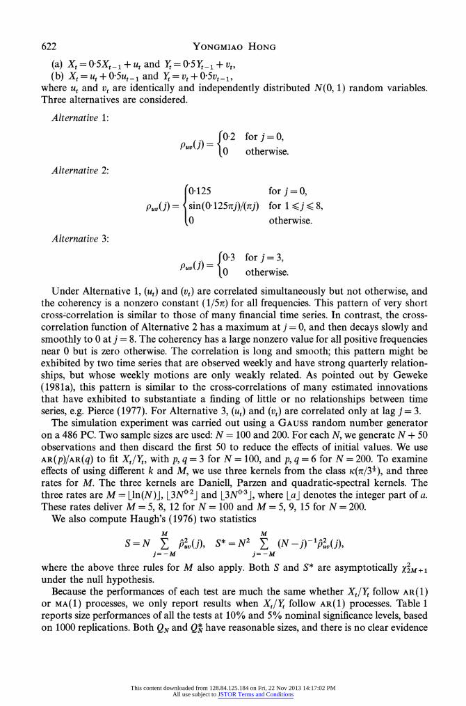
(a) X, = 05X,_1 + u, and Y= 0-5Y_1 + vt, (b) X,=u+ 05u_-1 and Y,=v+ 05v_-1,

where u, and v, are identically and independently distributed N(0, 1) random variables. Three alternatives are considered.

Alternative 1:

f0 2 for j = 0,

P J otherwise.

Alternative 2:

0r125 for j = 0, pUv(j)= sin(041257tj)/(ltj) for 1 ]j < 8,

10 otherwise. Alternative 3:

) 0-3 for j=3,

h 0 otherwise.

Under Alternative 1, (us) and (vi) are correlated simultaneously but not otherwise, and the coherency is a nonzero constant (1/57t) for all frequencies. This pattern of very short cross-correlation is similar to those of many financial time series. In contrast, the cross- correlation function of Alternative 2 has a maximum at j = 0, and then decays slowly and smoothly to 0 at j = 8. The coherency has a large nonzero value for all positive frequencies near 0 but is zero otherwise. The correlation is long and smooth; this pattern might be exhibited by two time series that are observed weekly and have strong quarterly relationships, but whose weekly motions are only weakly related. As pointed out by Geweke (1981a), this pattern is similar to the cross-correlations of many estimated innovations that have exhibited to substantiate a finding of little or no relationships between time series, e.g. Pierce (1977). For Alternative 3, (ut) and (v,) are correlated only at lag j = 3.

The simulation experiment was carried out using a GAUSS random number generator on a 486 PC. Two sample sizes are used: N = 100 and 200. For each N, we generate N + 50 observations and then discard the first 50 to reduce the effects of initial values. We use AR(P)/AR(q) to fit Xt/lY, with p, q = 3 for N = 100, and p, q = 6 for N = 200. To examine effects of using different k and M, we use three kernels from the class Kc(7/3'), and three rates for M. The three kernels are Daniell, Parzen and quadratic-spectral kernels. The three rates are M = Lln(N)i, L3N0 2i and L3N]3j, where Lai denotes the integer part of a. These rates deliver M = 5, 8, 12 for N = 100 and M = 5, 9, 15 for N = 200.

We also compute Haugh's (1976) two statistics M M

S=N A 2 (j)9 S* = N2 , (N-_j) lPA2(j)9

j=-M j=-M

where the above three rules for M also apply. Both S and S* are asymptotically X22M+1 under the null hypothesis.

Because the performances of each test are much the same whether Xt/IY follow AR(1) or MA(1) processes, we only report results when Xt/Yt follow AR(1) processes. Table 1 reports size performances of all the tests at 10% and 5% nominal significance levels, based on 1000 replications. Both QN and QN have reasonable sizes, and there is no clear evidence




Table 1. Rejection rates out of 1000 replications under the null hypothesis of independence, X, = 0 5X,1 + ut, Y, = 0 5Y + vt, where ut, v, - N(O, 1), and

P"v(j) =0 for all j N = 100 N = 200

M=5 M=8 M=12 M=5 M=9 M=15 10% 5% 10% 5% 10% 5% 10% 5% 10% 5% 10% 5%

QN DN 10.2 6-4 9-6 5-4 8.6 4-8 9-0 6-0 9-9 6-2 9-7 6-5 PZ 10.6 5-9 9-0 5-6 8-0 4-6 9.1 5-7 10-1 6-8 9-5 6-3 QS 10.4 6-2 9-3 5-5 8-1 5-0 8-8 5-5 8-5 5-5 8-8 5-7

QN DN 9-6 5-1 7-9 5-4 5-6 3-7 8-7 6-0 8-0 5-7 7-7 5-1 PZ 9-4 5-4 7-6 4-8 6-7 4-0 8-8 5-6 9-5 6-1 8-3 5-4 QS 10-0 5-6 8-5 5-0 6-5 4-1 8-8 5-5 8-5 5-5 8-8 5-7

S 7-8 3-6 6-5 2-2 3-9 1-1 8-3 4-4 7-7 3-7 6-7 2-7

S* 887 4-5 7-8 3-3 7-7 3-2 8-6 4-8 9-2 4-5 8-7 4-2

DN, Daniell kernel; Pz, Parzen kernel; QS, quadratic-spectral kernal.

favouring either one. At the 10% level, QN and QN have better sizes than S and S*. At the 5% level, QN and QN exhibit a little over-rejection in some cases, while S and S* exhibit a little under-rejection in some cases. The test S* has better size than S at both the 10% and 5% levels, especially for N = 100.

Table 2 reports power performances under Alternative 1 at the 5% level, based on 500 replications. We use both asymptotic and empirical critical values, the latter obtained from the 1000 replications under the null hypothesis. Both QN and QN perform similarly. The three kernels deliver similar power. For each kernel, the more slowly M grows, the better is the power of the test. In fact, because Alternative 1 is a simultaneous cross- correlation, including extra terms will sacrifice efficiency of the tests. On the other hand, S and S* perform similarly, and smaller M gives better power. We see that QN and QN are about twice as powerful as Haugh's tests.

Table 2. Rejection rates out of 500 replications at the 5% level under Alternative 1: X= 0-5X,_1 + u, Y= 0-5Y + vt, where ut, vt - N(0,1), PUV(O) = 0 2 and p.,(j)=

Ofor all j $ 0

N = 100 N = 200 M=5 M=8 M=12 M=5 M=9 M=15

ACV ECV ACV ECV ACV ECV ACV ECV ACV ECV ACV ECV

QN DN 38-8 35-4 29-0 28-4 24-0 24-6 66-6 62-4 55-8 51-8 44-4 40-4 PZ 37-0 32-6 28-8 27-2 23-8 25-2 65-0 63-4 54-4 50-2 42-8 38-4 QS 39-0 34-2 29-4 27-8 24-6 24-6 66-8 64-4 55-8 53-0 44-4 40-2

QN DN 36-6 35-2 26-8 28-4 19-2 24-6 65-8 62-2 53-6 52-0 40-8 40-6 PZ 36-0 32-6 26-0 27-2 20-6 25-2 64-6 63-4 52-8 50-2 39-8 38-4 QS 36-6 34-2 27-8 27-8 21-4 24-6 65-8 64-4 54-6 53-0 42-6 40-0

S 13-4 16-2 10.4 16-4 6-0 15-2 35-0 36-8 24-0 28-8 17-6 23-6

S* 14-4 15-8 12-8 15-8 10.6 14-6 35-8 36-0 26-6 28-0 21-4 22-4

DN, Daniell kernel; PZ, Parzen kernel; QS, quadratic-spectral kernel; ACV, asymptotic critical value; ECV, empirical critical value.



624 YONGMIAO HONG

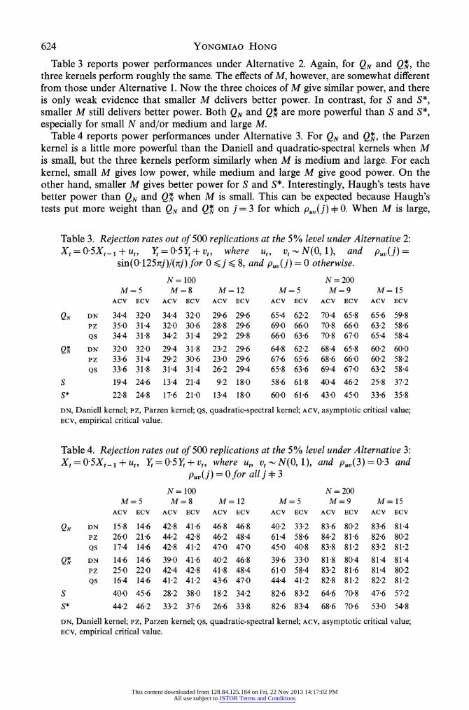
Table 3 reports power performances under Alternative 2. Again, for QN and QN, the three kernels perform roughly the same. The effects of M, however, are somewhat different from those under Alternative 1. Now the three choices of M give similar power, and there is only weak evidence that smaller M delivers better power. In contrast, for S and S*, smaller M still delivers better power. Both QN and QN are more powerful than S and S*, especially for small N and/or medium and large M.

Table 4 reports power performances under Alternative 3. For QN and QN, the Parzen kernel is a little more powerful than the Daniell and quadratic-spectral kernels when M is small, but the three kernels perform similarly when M is medium and large. For each kernel, small M gives low power, while medium and large M give good power. On the other hand, smaller M gives better power for S and S*. Interestingly, Haugh's tests have better power than QN and Q* when M is small. This can be expected because Haugh's tests put more weight than QN and Q* on j = 3 for which pUV(j) 0 O. When M is large,

Table 3. Rejection rates out of 500 replications at the 5% level under Alternative 2: Xt= 0-5Xt_1 + ut, Yt = 0 5Yt + vt, where ut, vt - N(0, 1), and pU(;) =

sin(0 1252tj)/(2tj) for 0 < j < 8, and pUV(j) = 0 otherwise.

N = 100 N = 200 M=5 M=8 M=12 M=5 M=9 M=15

ACV ECV ACV ECV ACV ECV ACV ECV ACV ECV ACV ECV

QN DN 34-4 32-0 34-4 32-0 29-6 29-6 65-4 62-2 70-4 65-8 65-6 59-8 PZ 35-0 31-4 32-0 30-6 28-8 29-6 69-0 66-0 70-8 66.0 63-2 58-6 QS 34-4 31F8 34-2 31-4 29.2 29-8 66.0 63-6 70.8 67-0 65-4 58-4

QN DN 32-0 32-0 29-4 31-8 23.2 29-6 64-8 62-2 68.4 65-8 60-2 60-0 PZ 33-6 31-4 29-2 30.6 23-0 29-6 67.6 65-6 68&6 66-0 60.2 58-2 QS 33-6 31-8 31V4 31-4 26-2 29-4 65-8 63-6 69.4 67-0 63-2 58-4

S 19-4 24-6 13-4 2194 9-2 18&0 58-6 6198 40.4 46-2 25-8 37-2

S* 22-8 24-8 17-6 21.0 13-4 18-0 60-0 61-6 43.0 45.0 33.6 35-8

DN, Daniell kernel; Pz, Parzen kernel; QS, quadratic-spectral kernel; ACV, asymptotic critical value; ECV, empirical critical value.

Table 4. Rejection rates out of 500 replications at the 5% level under Alternative 3: Xt= 0 5Xt-, + ut, t = 0 5Yt + vt, where ut, vt N(0, 1), and p.,(3) = 0-3 and

P.v(j) = O for all j 3 N = 100 N = 200

M=5 M=8 M=12 M=5 M=9 M=15 ACV ECV ACV ECV ACV ECV ACV ECV ACV ECV ACV ECV

QN DN 15-8 14-6 42.8 41-6 46-8 46-8 40-2 33-2 83-6 80.2 83-6 81-4 PZ 26-0 21-6 44-2 42.8 46-2 48-4 61-4 58.6 84.2 8196 82-6 80-2 QS 17-4 14-6 42-8 41-2 47.0 47-0 45-0 40-8 83-8 8192 83-2 8192

QN DN 14-6 14-6 39-0 41-6 40-2 46-8 39-6 33-0 81-8 80-4 81-4 81-4 PZ 25-0 22-0 42-4 42-8 4198 48-4 6190 58.4 83-2 8196 8194 80-2 QS 16-4 14-6 41-2 41-2 43-6 47-0 44.4 4192 82-8 8192 82-2 8192

S 40-0 45-6 28-2 38-0 18-2 34-2 82.6 83.2 64-6 70-8 47-6 57-2

S* 44-2 46-2 33-2 37-6 26-6 33-8 82-6 83-4 68-6 70-6 53-0 54-8

DN, Daniell kernel; PZ, Parzen kernel; QS, quadratic-spectral kernel; ACV, asymptotic critic allue; ECV, empirical critical value.




however, Haugh's tests become less powerful than QN and QN. This is because, although Haugh's tests put more weight on j = 3, they also, inefficiently, put more weights than QN and QN on many lags for which p.,(j) = 0.

In summary, the simulation study shows that the new tests perform reasonably well, having good power against short and long cross-correlations. Different choices of kernel, other than the truncated kernel, give similar power. In most cases, the new tests have better power than Haugh's tests or the truncated kernel based tests.

ACKNOWLEDGEMENT

I would like to thank a referee, an Associate Editor, the Editor, D. Easley, J. Geweke, G. Jakubson, N. Kiefer, H. Pesaran and M. Wells for providing useful comments. The research was carried out with a faculty research summer support from the Department of Economics, Cornell University.

REFERENCES

ANDREWS, D. W. K. (1991). Heteroskedasticity and autocorrelation consistent covariance matrix estimation. Econometrica 59, 817-58.

BAHADUR, R. R. (1960). Stochastic comparison of tests. Ann. Math. Statist. 31, 276-95. BERK, K. N. (1974). Consistent autoregressive spectral estimates. Ann. Statist. 2, 489-502. CHAN, N. H. & TRAN, L. T. (1992). Nonparametric tests for serial dependence. J. Time Ser. Anal. 13, 102-13. GALLANT, A. R. & JORGENSON, D. (1979). Statistical inference for a system of simultaneous nonlinear implicit

equations in the context of instrumental variables estimation. J. Economet. 11, 275-302. GALLANT, A. R. & WHITE, H. (1988). A Unified Theory of Estimation and Inference for Nonlinear Dynamic

Models. Oxford: Basil Blackwell. GEWEKE, J. (1981a). The approximate slopes of econometric tests. Econometrica 49, 1427-42. GEWEKE, J. (1981b). A comparison of tests of independence of two covariance stationary time series. J. Am.

Statist. Assoc. 76, 363-73. HAUGH, L. D. (1976). Checking the independence of two covariance-stationary time series: a univariate

residual cross correlation approach. J. Am. Statist. Assoc. 71, 378-85. HONG, Y. (1996). Consistent testing for serial correlation of unknown form. Econometrica 64, 837-64. PIERCE, A. (1977). Lack of dependence among economic variables. J. Am. Statist. Assoc. 72, 11-22. PITMAN, E. J. G. (1979). Some Basic Theory for Statistical Inference. London: Chapman Hall. PRIESTLEY, M. B. (1962). Basic considerations in the estimation of spectra. Technometrics 4, 551-64. PRIESTLEY, M. B. (1981). Spectral Analysis and Time Series, 1, 2. London: Academic Press. ROBINSON, P. M. (1991). Consistent nonparametric entropy-based testing. Rev. Econ. Studies 58, 437-53. SKAUG, H. J. & TJOSTHEIM, D. (1993a). A nonparametric test of serial independence based on the empirical

distribution function. Biometrika 80, 591-602. SKAUG, H. J. & TJOSTHEIM, D. (1993b). Nonparametric tests of serial independence. In Developments in Time

Series Analysis, the M. B. Priestley Birthday Volume, Ed. T. Subba Rao, pp. 207-29. London: Academic Press.

[Received August 1994. Revised August 1995]



testing for independence between two covariance stationary ... for independence... · biometrika...

Documents