Testing and Validating Machine Learning Classifiers byMetamorphic TestingI

Xiaoyuan Xiea,d,e,∗, Joshua W. K. Hob, Christian Murphyc, Gail Kaiserc,Baowen Xue, Tsong Yueh Chena

aCentre for Software Analysis and Testing, Swinburne University, Hawthorn, Vic 3122 AustraliabSchool of Information Technologies, The University of Sydney, NSW 2006, Australia; and

NICTA, Australian Technology Park, Eveleigh, NSW 2015, AustraliacDepartment of Computer Science, Columbia University, New York NY 10027 USA

dSchool of Computer Science and Engineering, Southeast University, Nanjing 210096, ChinaeState Key Laboratory for Novel Software Technology &

Department of Computer Science and Technology, Nanjing University, Nanjing 210093, China

Abstract

Machine Learning algorithms have provided important core functionality tosupport solutions in many scientific computing applications - such as computa-tional biology, computational linguistics, and others. However, it is difficult totest such applications because often there is no “test oracle” to indicate what thecorrect output should be for arbitrary input. To help address the quality of sci-entific computing software, in this paper we present a technique for testing theimplementations of machine learning classification algorithms on which such sci-entific computing software depends. Our technique is based on an approach called“metamorphic testing”, which has been shown to be effective in such cases. Alsopresented is a case study on a real-world machine learning application framework,and a discussion of how programmers implementing machine learning algorithmscan avoid the common pitfalls discovered in our study. We also conduct muta-tion analysis and cross-validation, which reveal that our method has very high

IA preliminary version of this paper was presented at the 9th International Conference onQuality Software (QSIC 2009) (Xie et al., 2009).

∗Corresponding author. Tel.: +61.3.9214.8678; fax: +61.3.9819.0823.Email addresses: xxie@groupwise.swin.edu.au (Xiaoyuan Xie),

joshua@it.usyd.edu.au (Joshua W. K. Ho), cmurphy@cs.columbia.edu (ChristianMurphy), kaiser@cs.columbia.edu (Gail Kaiser), bwxu@nju.edu.cn (Baowen Xu), tychen@groupwise.swin.edu.au (Tsong Yueh Chen)

Preprint submitted to Elsevier January 11, 2010

CORE Metadata, citation and similar papers at core.ac.uk

Provided by Columbia University Academic Commons

effectiveness in killing mutants, and that observing expected cross-validation re-sult alone is not sufficient to test for the correctness of a supervised classificationprogram. Metamorphic testing is strongly recommended as a complementary ap-proach. Finally we discuss how our findings can be used in other areas of compu-tational science and engineering.

Keywords: Metamorphic Testing, Machine Learning, Test Oracle, OracleProblem, Validation, Verification

1. Introduction

Machine Learning algorithms have provided important core functionality tosupport solutions in many scientific computing applications - such as computa-tional biology, computational linguistics, and others. For instance, there are overfifty different real-world applications in computational science, ranging from fa-cial recognition to computational biology, which use the Support Vector Machinesclassification algorithm alone (SVM Application List, 2006) . As these types ofapplications become more and more prevalent in society (Mitchell, 1983), ensur-ing their quality becomes more and more crucial.

Quality assurance of such applications presents a challenge because conven-tional software testing processes do not always apply: in particular, it is difficultto detect subtle errors, faults, defects or anomalies in many applications in thesedomains because there is no reliable “test oracle” to indicate what the correctoutput should be for arbitrary input. The general class of software systems withno reliable test oracle available is sometimes known as “non-testable programs”(Weyuker, 1982). Many of these applications fall into a category of software thatWeyuker describes as “Programs which were written in order to determine theanswer in the first place. There would be no need to write such programs, if thecorrect answer were known” (Weyuker, 1982).

The majority of the research effort in the domain of machine learning focuseson building more accurate models that can better achieve the goal of automatedlearning from the real world. However, to date very little work has been done onassuring the correctness of the software applications that perform machine learn-ing. Formal proofs of an algorithm’s optimal quality do not guarantee that anapplication implements or uses the algorithm correctly, and thus software testingis necessary.

To help address the quality of scientific computing software, this paper presentsa technique for testing implementations of the supervised machine learning algo-

rithms on which such software depends. Our technique is based on an approachcalled “metamorphic testing” (Chen et al., 1998), which uses properties of func-tions such that it is possible to predict expected changes to the output for particularchanges to the input, based on so-called “metamorphic relations” between sets ofinputs and their corresponding outputs. Although the correct output cannot beknown in advance, if the change is not as expected, then a defect must exist.

In our approach, we first enumerate the metamorphic relations that such algo-rithms would be expected to demonstrate, then for a given implementation deter-mine whether each relation is a necessary property to reveal program correctness.If it is, then failure to exhibit the relation indicates a defect, that is, they can beused for the purpose of testing. If it is not a necessary property, that is, althoughthese properties would still be anticipated to hold in the classification algorithmswe investigate, some of them could conceivably be violated without indicating adefect in the implementation, they can instead be used for validation. In such case,a violation of the property may or may not indicate a defect, but still represents adeviation from “expected” behavior.

In addition to presenting our technique, we describe a case study we per-formed on the real-world machine learning application framework Weka (Wittenand Frank, 2005), which is used as the foundation for such computational sciencetools as BioWeka (Gewehr et al., 2007) in bioinformatics. We also discuss howour findings can be of use to other areas of computational science and engineering,such as computational linguistics.

The rest of this paper is organized as follows: Section 2 supplies backgroundinformation about machine learning and introduces the specific algorithms thatare evaluated. Section 3 discusses the metamorphic testing approach and the spe-cific metamorphic relations used for testing machine learning classifiers. Section4 presents the results of case studies demonstrating that the approach can find de-fects in real-world machine learning applications. Section 5 discusses empiricalstudies that use mutation testing to systematically insert defects into the sourcecode, and measures the effectiveness of metamorphic testing. Section 6 presentsrelated work, and Section 7 concludes.

2. Background

In this section, we present some of the basics of machine learning and the twoalgorithms we investigated (k-Nearest Neighbors and Naıve Bayes Classifier) (wepreviously considered Support Vector Machines in Murphy et al. (2008)), as well

as the terminology used. Readers familiar with machine learning may skip thissection.

One complication in our work arose due to conflicting technical nomenclature:“testing”, “regression”, “validation”, “model” and other relevant terms have verydifferent meanings to machine learning experts than they do to software engineers.Here we employ the terms “testing”, “regression testing”, and “validation” as ap-propriate for a software engineering audience, but we adopt the machine learningsense of “model”, as defined below.

2.1. Machine Learning FundamentalsIn general, input to a supervised machine learning application consists of a set

of training data that can be represented by two vectors of size k. One vector is forthe k training samples S = <s0, s1, ..., sk-1> and the other is for the correspondingclass labels C = <c0, c1, ..., ck-1>. Each sample s ∈ S is a vector of size m, whichrepresents m features from which to learn. Each label ci in C is an element of afinite set of class labels, that is, c ∈ L = {l0, l1, ..., ln-1}, where n is the number ofpossible class labels.

27,81,88,59,15,16,88,82,41,17,81,98,42, ..., 015,70,91,41, 5, 3,65,27,82,64,58,29,19, ..., 022,72,11,92,96,24,44,92,55,11,12,44,84, ..., 182, 3,51,47,73, 4, 1,99, 1,51,84, 1,41, ..., 057,77,33,86,89,77,61,76,96,98,99,21,62, ..., 1...

Figure 1: Example of part of a data set used by supervised ML classifier algorithms

Figure 1 shows a small portion of a training data set that could be used bysupervised learning applications. The rows represent samples from which to learn,as comma-separated attribute values; the last number in each row is the label.

Supervised ML applications consist of two phases. The first phase (called thetraining phase) analyzes the training data; the result of this analysis is a modelthat attempts to make generalizations about how the attributes relate to the label.In the second phase (called the testing phase), the model is applied to another,previously-unseen data set (the testing data) where the labels are unknown. In aclassification algorithm, the system attempts to predict the label of each individualexample. That is, the testing data input is an unlabeled test case ts, and the aim isto determine its class label ct based on the data-label relationship learned from theset of training samples S and the corresponding class labels C, where ct ∈ L.

2.2. Algorithms InvestigatedThis paper only investigates supervised learning applications. Within the area

of supervised learning, we particularly focus on programs that perform classifica-tion, since classification is one of the central tasks in machine learning. The workpresented here has focused on the k-Nearest Neighbors classifier and the NaıveBayes Classifier, which were chosen because of their extensive use throughoutthe ML community. However, it should be noted that the problem description andtechniques described below are not specific to any particular algorithm, and asshown in our previous work (Chen et al., 2009; Murphy et al., 2008), our resultsare applicable to the general case.

In k-Nearest Neighbors (kNN), for a training sample set S, suppose each sam-ple has m attributes, <att0, att1, ..., attm-1>, and there are n classes in S, {l0, l1,..., ln-1}. The value of the test case ts is <a0, a1, ..., am-1>. kNN computes thedistance between each training sample and the test case. Generally kNN uses theEuclidean Distance: for a sample si ∈ S, the value of each attribute is <sa0, sa1,..., sam-1>, and the distance formula is as follows:

dist(si, ts) =

√√√√m−1∑j

(saj − aj)2.

After sorting all the distances, kNN selects the k nearest ones and these sam-ples are considered the k nearest neighbors of the test case. Then kNN calculatesthe proportion of each label in the k nearest neighbors, and the label with thehighest proportion is assigned as the label of the test case.

In the Naıve Bayes Classifier (NBC), for a training sample set S, supposeeach sample has m attributes, <att0, att1, ..., attm-1>, and there are n classes in S,{l0, l1, ..., ln-1}. The value of the test case ts is <a0, a1, ..., am-1>. The label of ts iscalled lts, and is to be predicted by NBC.

NBC computes the probability of lts belonging to lk, when each attribute valueof ts is <a0, a1, ..., am>. NBC assumes that attributes are conditionally indepen-dent with one another given the class label, therefore we have the equation:

P(lts = lk | a0a1...am-1) =

P(lk)∏j

P(aj | lts = lk)∑iP(li)

∏jP(aj|lts = li)

After computing the probability for each li ∈ {l0, l1, ..., ln-1}, NBC assigns thelabel lk with the highest probability, as the label of test case ts.

Generally NBC uses a normal distribution to compute P(aj | lts = lk). ThusNBC trains the training sample set to establish a distribution function for eachelement attj of vector <att0, att1, ..., attm-1> in each li ∈ {l0, l1, ..., ln-1}, that is,

for all samples with label li ∈ {l0, l1, ..., ln-1}, it calculates the mean value µ andmean square deviation σ of attj in all samples with li. Then a probability densityfunction is constructed for a normal distribution with µ and σ.

For test case ts with m attribute values <a0, a1, ..., am-1>, NBC computes theprobability of P(aj | lts = lk) using a small interval δ to calculate the integral area.With the above formulae NBC can then compute the probability of lts belongingto each li and choose the label with the highest probability as the classification ofts.

3. Approach

Our approach is based on the concept of metamorphic testing (Chen et al.,1998), summarized below. To facilitate that approach, we must identify the rela-tions that the algorithms are expected to exhibit between sets of inputs and setsof outputs. Once those relations have been determined, we then analyze the al-gorithms to decide whether the relations are necessary properties to indicate cor-rectness during testing; that is to say, if the implementation does not exhibit thatproperty, then there is a defect. If the relation is not a necessary property, it canstill be used for for the purpose of validation, that is, whether the algorithm satisiesthe requirement.

3.1. Metamorphic TestingOne popular technique for testing programs without a test oracle is to use a

“pseudo-oracle” (Davis and Weyuker, 1981), in which multiple implementationsof an algorithm process the same input and the results are compared; if the resultsare not the same, then one or both of the implementations contains a defect. Thisis not always feasible, though, since multiple implementations may not exist, orthey may have been created by the same developers, or by groups of developerswho are prone to making the same types of mistakes (Knight and Leveson, 1986).

However, even without multiple implementations, often these applications ex-hibit properties such that if the input were modified in a certain way, it shouldbe possible to predict the new output, given the original output. This approachis known as metamorphic testing. Metamorphic testing can be implemented veryeasily in practice. The first step is to identify a set of properties (“metamorphicrelations”, or MRs) that relate multiple pairs of inputs and outputs of the targetprogram. Then, pairs of source test cases and their corresponding follow-up test

cases are constructed based on these MRs. We then execute all these test cases us-ing the target program, and check whether the outputs of the source and follow-uptest cases satisfy their corresponding MRs.

A simple example of a function to which metamorphic testing could be appliedwould be one that calculates the standard deviation of a set of numbers. Certaintransformations of the set would be expected to produce the same result. Forinstance, permuting the order of the elements should not affect the calculation;nor would multiplying each value by -1, since the deviation from the mean wouldstill be the same.

Furthermore, there are other transformations that will alter the output, but ina predictable way. For instance, if each value in the set is multiplied by 2, thenthe standard deviation should be twice as much as that of the original set, sincethe values on the number line are just “stretched out” and their deviation fromthe mean becomes twice as great. Thus, given one set of numbers (the sourcetest cases), we can use these metamorphic relations to create three more sets offollow-up test cases (one with the elements permuted, one with each multipliedby -1, and another with each multiplied by 2); moreover, given the result of onlythe source test case, we can predict the others.

It is not hard to see that metamorphic testing is simple to implement, effective,easily automatable, and independent of any particular programming language.Further, for the identification of the MRs, which is the most crucial step in meta-morphic testing, there are several principles of both white-box and black-box canbe followed, such as, logical hierarchy, difference in execution traces, user’s pro-files, etc (Chen et al., 2004).

For example, based on the principle of “difference in execution traces”, we in-tend to select MRs with more differences between the execution traces of sourcetest cases and follow-up test cases. Here is an illustration: the Shortest-Path pro-gram SP accepts 3 parameters as inputs: a given graph G, a starting node s, andan ending node e. SP(G, s, e) returns the shortest path between s and e. Let usconsider the two following MRs as examples: MR1: | SP(G, s, e)| = | SP(G, s,m)| + | SP(G, m, e)|, where m denotes a visited node between s and e returnedby SP(G, s, e). And MR2: | SP(G, s, e)| = | SP(G, e, s)|. Apparently, these twoMRs will execute different path-pairs (source path and follow-up path), and a pathpair with more difference is preferred as a better MR. Of course in order to decidewhich MR will result in more execution difference, we can just run the programand collect the real coverage information. But we also can acquire this informa-tion simply by analysing the mechanism of the algorithm, without any execution.Suppose the algorithm is a forward-search algorithm, MR2 is likely to lead to

more execution difference. However if the algorithm is a 2-way search method,MR2 will not necessarily yield more execution difference.

Apart from the above principles, we can also harness the domain knowledge.This is a useful feature since in scientific computing the programmer may, in fact,also be the domain expert and will know what properties of the program will beused more heavily or are more critical. Perhaps more importantly, it is clear thatmetamorphic testing can be very useful in the absence of a test oracle, that is,when the correct output cannot be verified: regardless of the input values, if themetamorphic relations are violated, then there is likely a defect in the implemen-tation.

3.2. Metamorphic RelationsIn previous work (Murphy et al., 2008), we broadly classified six types of

metamorphic relations (MRs) applicable in general to many different types ofmachine learning applications, including both supervised and unsupervised ML.In this work, however, our approach calls for focusing on the specific metamorphicrelations of the application under test; we would expect that we could then createmore follow-up test cases and conceivably reveal more defects than by using moregeneral MRs. In particular, we define the MRs that we anticipate classificationalgorithms to exhibit, and define them more formally as follows.

MR-0: Consistence with affine transformation. The result should be thesame if we apply the same arbitrary affine transformation function, f(x) = kx + b,(k 6= 0) to every value x to any subset of features in the training data set S and thetest case ts.

MR-1.1: Permutation of class labels. Assume that we have a class-labelpermutation function Perm() to perform one-to-one mapping between a class labelin the set of labels L to another label in L. If the source case result is li, applying thepermutation function to the set of corresponding class labels C for the follow-upcase, the result of the follow-up case should be Perm(li).

MR-1.2: Permutation of the attribute. If we permute the m attributes of allthe samples and the test data, the result should remain unchanged.

MR-2.1: Addition of uninformative attributes. An uninformative attributeis one that is equally associated with each class label. For the source input, sup-pose we get the result ct = li for the test case ts. In the follow-up input, we addan uninformative attribute to S and respectively a new attribute in st. The choiceof the actual value to be added here is not important as this attribute is equallyassociated with the class labels. The output of the follow-up test case should stillbe li.

MR-2.2: Addition of informative attributes. For the source input, supposewe get the result ct = li for the test case ts. In the follow-up input, we add aninformative attribute to S and ts such that this attribute is strongly associated withclass li and equally associated with all other classes. The output of the follow-uptest case should still be li.

MR-3.1: Consistence with re-prediction. For the source input, suppose weget the result ct = li for the test case ts. In the follow-up input, we can append ts

and ct to the end of S and C respectively. We call the new training dataset S’ andC’. We take S’, C’ and ts as the input of the follow-up case, and the output shouldstill be li.

MR-3.2: Additional training sample. For the source input, suppose we getthe result ct = li for the test case ts. In the follow-up input, we duplicate all samplesin S and L which have label li. The output of the follow-up test case should stillbe li.

MR-4.1: Addition of classes by duplicating samples. For the source input,suppose we get the result ct = li for the test case ts. In the follow-up input, weduplicate all samples in S and C that do not have label li and concatenate anarbitrary symbol “*” to the class labels of the duplicated samples. That is, ifthe original training set S is associated with class labels <A, B, C> and li is A, theset of classes in S in the follow-up input could be <A, B, C, B*, C*>. The outputof the follow-up test case should still be li. Another derivative of this metamorphicrelation is that duplicating all samples from any number of classes which do nothave label li will not change the result of the output of the follow-up test case.

MR-4.2: Addition of classes by re-labeling samples. For the source input,suppose we get the result ct = li for the test case ts. In the follow-up input, we re-label some of the samples in S and C which have label other than li and concatenatean arbitrary symbol “*” to their class labels. That is, if the original training set Sis associated with class labels <A, B, B, B, C, C, C> and c0 is A, the set of classesin S in the follow-up input may become <A, B, B, B*, C, C*, C*>. The output ofthe follow-up test case should still be li.

MR-5.1: Removal of classes. For the source input, suppose we get the resultct = li for the test case ts. In the follow-up input, we remove one entire class ofsamples in S of which the label is not li. That is, if the original training set S isassociated with class labels <A, A, B, B, C, C> and li is A, the set of classes inS in the follow-up input may become <A, A, B, B>. The output of the follow-uptest case should still be li.

MR-5.2: Removal of samples. For the source input, suppose we get the resultct = li for the test case ts. In the follow-up input, we remove part of some of the

samples in S and C of which the label is not li. That is, if the original training set Sis associated with class labels <A, A, B, B, C, C> and li is A, the set of classes inS in the follow-up input may become <A, A, B, C>. The output of the follow-uptest case should still be li.

3.3. Analysis of Relations for ClassifiersWe do not formally prove here that all of these properties hold for both the

kNN and NBC. Rather, we demonstrate here that some of the relations are not,necessary properties of the algorithms being implemented. For those MRs whichare necessary properties, we can use them in software testing, but for the MRsdemontrated as follows, we can still use them for the purpose of validation.

For kNN, five of the above metamorphic relations are not necessary propertiesbut can instead be used for validation purposes. MR-1.1 (Permutation of classlabels) is not a necessary property because of tiebreaking between two labels forprediction that are equally likely: permuting their order may change which one ischosen by the tiebreaker.

Additionally, MR-5.1 (Removal of classes) is not a necessary property. Sup-pose the predicted label of the test case is li. MR-5.1 removes a whole class ofsamples without label li. Consequently this will remove the same samples in theset of k nearest neighbors, and thus some other samples will be included in the setof k nearest neighbors. These samples may have any labels except the removedone, and so the likelihood of any label (except the removed one) may increase.Therefore there are two situations: (1) If in the k nearest neighbors of the sourcecase, the proportion of li is not only the highest, but also higher than 50%, thenin the follow-up prediction, no matter how the k nearest neighbors change, thepredication will remain the same, because no matter which labels increase, theproportion of li will still be higher than 50% as well. Thus the prediction remainsli. Now consider situation (2), in which in the k nearest neighbors of the sourcecase, the proportion of li is the highest but lower or equal to 50%. Since the num-ber of each survived label may increase, and the original proportion of li is loweror equal to 50%, it is possible that the proportion of some other label increasesand becomes higher than li: thus, the prediction changes.

Similarly MR-2.2 (Addition of informative attributes), MR-4.1 (Addition ofclasses by duplicating samples), and MR-5.2 (Removal of samples) may not holdif the predicted label has a likelihood of less than 50%.

For the NBC, three of the metamorphic relations are not considered neces-sary properties, but can still be used for validation: MR-3.1 (Consistence withre-prediction), MR-4.2 (Addition of classes by re-labeling samples), and MR-5.2

(Removal of samples). MR-3.1 could not be proven as a necessary property, andthus is considered not necessary; the other two introduce noise to the data set,which could affect the result.

4. Case Studies

To demonstrate the effectiveness of metamorphic testing in validating machinelearning applications, we applied the approach to Weka 3.5.7 (Witten and Frank,2005). Weka is a popular open-source machine learning package that implementsmany common algorithms for data preprocessing, classification, clustering, asso-ciation rule mining, feature selection and visualization. Due to its large rangeof functionality, it is typically used as a “workbench” for applying various ma-chine learning algorithms. Furthermore, Weka is widely used as the back-endmachine learning engine for various applications in computational science, suchas BioWeka (Gewehr et al., 2007) for machine learning tasks in bioinformatics.

4.1. Experimental SetupThe data model in our experiments is as follows. In one source suite, there

are k inputs. Each input i has two parts: tr i and t i, in which tr i represents thetraining sample set, and t i represents the test case. In each training sample settr i and test case t i, there are four attributes: <A0, A1, A2, A3>, and a label L. Inour experiments, there are three labels, that is, {L0, L1, L2}. The value for eachattribute is within [1, 20]. We generate the tr i and t i values randomly, both in thevalue of the attribute and the label. The number of samples in tr i is also randomlygenerated with a maximum of n.

This randomly generated data model does not encapsulate any domain knowl-edge, that is, we do not use any meaningful, existing training data for testing: eventhough those data sets are more predictable, they may not be sensitive to detectingfaults. Random data may, in fact, be more useful at revealing defects (Duran andNtafos, 1984).

For the source suite of k inputs, we perform a transformation according to theMRs and get k follow-up inputs for each MR-j. From running the k follow-upinputs and comparing the results between the source and the follow-up cases forthe each MR-j, we try to detect faults in Weka or find a violation between theclassifier under test and the anticipated properties of the classifier.

For each MR-j, we conducted several batches of experiments, and in eachbatch of experiments we changed the value of k (size of source suite) and n (maxnumber of training samples). Intuitively the more inputs we tried (the higher is k),

the more likely we are to find violations. Also, we would expect that with fewersamples in the training data set (the less is n), the less predictable the data are,thus the more likely we are to find faults.

4.2. FindingsOur investigation into the kNN and NBC implementations in Weka revealed

that some NBC test cases caused violations in the necessary properties, indicatingdefects. In other cases, for both algorithms, metamorphic relations that could beused for validation were also violated, perhaps not indicating an actual defect butshowing that the implementations could yield unexpected results and deviate fromthe behavior anticipated by scientific computing users.

4.2.1. k-Nearest NeighborsNone of the necessary properties of kNN were violated by our testing, but we

did uncover violations in some of the other properties used during validation. Al-though these are not necessarily indicative of defects per se, they do demonstratea deviation from what would normally be considered the expected behavior.

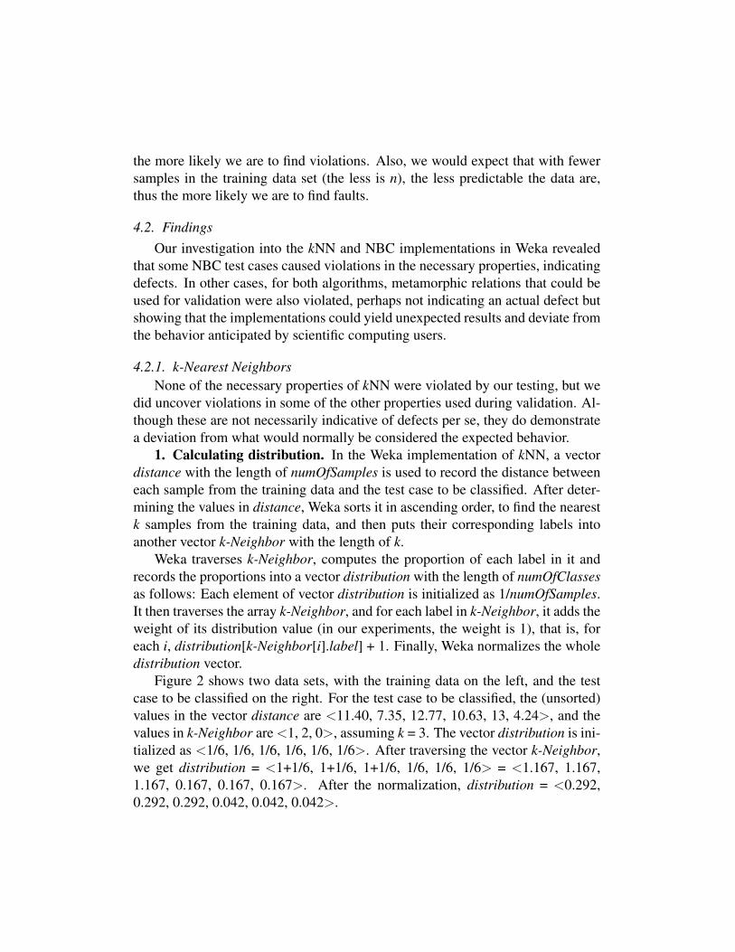
1. Calculating distribution. In the Weka implementation of kNN, a vectordistance with the length of numOfSamples is used to record the distance betweeneach sample from the training data and the test case to be classified. After deter-mining the values in distance, Weka sorts it in ascending order, to find the nearestk samples from the training data, and then puts their corresponding labels intoanother vector k-Neighbor with the length of k.

Weka traverses k-Neighbor, computes the proportion of each label in it andrecords the proportions into a vector distribution with the length of numOfClassesas follows: Each element of vector distribution is initialized as 1/numOfSamples.It then traverses the array k-Neighbor, and for each label in k-Neighbor, it adds theweight of its distribution value (in our experiments, the weight is 1), that is, foreach i, distribution[k-Neighbor[i].label] + 1. Finally, Weka normalizes the wholedistribution vector.

Figure 2 shows two data sets, with the training data on the left, and the testcase to be classified on the right. For the test case to be classified, the (unsorted)values in the vector distance are <11.40, 7.35, 12.77, 10.63, 13, 4.24>, and thevalues in k-Neighbor are<1, 2, 0>, assuming k = 3. The vector distribution is ini-tialized as <1/6, 1/6, 1/6, 1/6, 1/6, 1/6>. After traversing the vector k-Neighbor,we get distribution = <1+1/6, 1+1/6, 1+1/6, 1/6, 1/6, 1/6> = <1.167, 1.167,1.167, 0.167, 0.167, 0.167>. After the normalization, distribution = <0.292,0.292, 0.292, 0.042, 0.042, 0.042>.

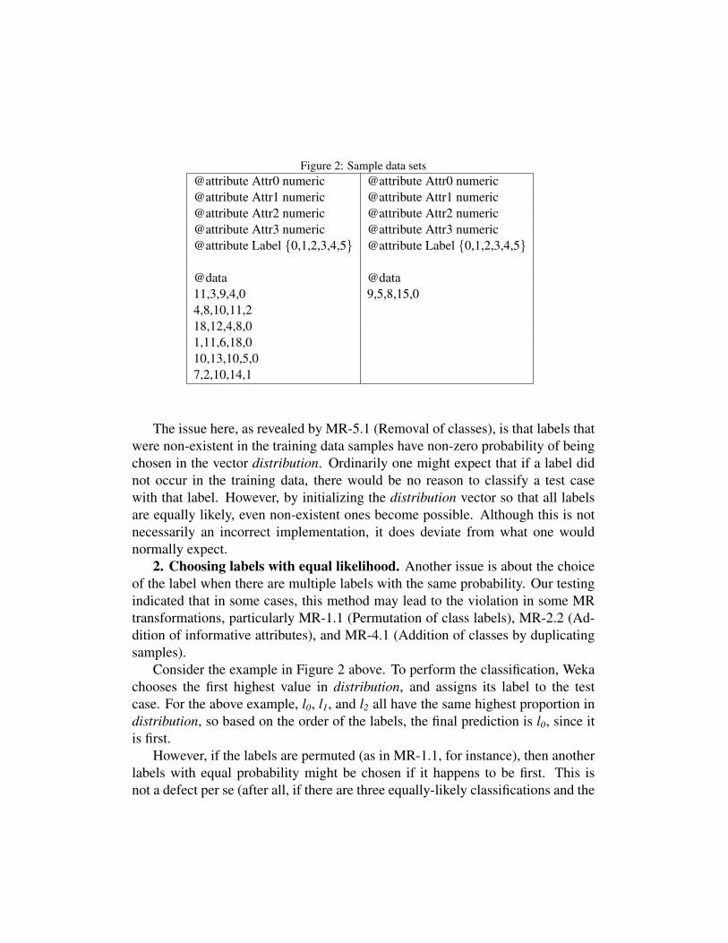
Figure 2: Sample data sets@attribute Attr0 numeric @attribute Attr0 numeric@attribute Attr1 numeric @attribute Attr1 numeric@attribute Attr2 numeric @attribute Attr2 numeric@attribute Attr3 numeric @attribute Attr3 numeric@attribute Label {0,1,2,3,4,5} @attribute Label {0,1,2,3,4,5}

@data @data11,3,9,4,0 9,5,8,15,04,8,10,11,218,12,4,8,01,11,6,18,010,13,10,5,07,2,10,14,1

The issue here, as revealed by MR-5.1 (Removal of classes), is that labels thatwere non-existent in the training data samples have non-zero probability of beingchosen in the vector distribution. Ordinarily one might expect that if a label didnot occur in the training data, there would be no reason to classify a test casewith that label. However, by initializing the distribution vector so that all labelsare equally likely, even non-existent ones become possible. Although this is notnecessarily an incorrect implementation, it does deviate from what one wouldnormally expect.

2. Choosing labels with equal likelihood. Another issue is about the choiceof the label when there are multiple labels with the same probability. Our testingindicated that in some cases, this method may lead to the violation in some MRtransformations, particularly MR-1.1 (Permutation of class labels), MR-2.2 (Ad-dition of informative attributes), and MR-4.1 (Addition of classes by duplicatingsamples).

Consider the example in Figure 2 above. To perform the classification, Wekachooses the first highest value in distribution, and assigns its label to the testcase. For the above example, l0, l1, and l2 all have the same highest proportion indistribution, so based on the order of the labels, the final prediction is l0, since itis first.

However, if the labels are permuted (as in MR-1.1, for instance), then anotherlabels with equal probability might be chosen if it happens to be first. This isnot a defect per se (after all, if there are three equally-likely classifications and the

function needs to return only one, it must choose somehow) but rather it representsa deviation from expected behavior (that is, the order of the data set shall not affectthe computed outputs), one that could have an effect on an application using thisfunctionality.

4.2.2. Naıve Bayes ClassifierOur investigation into NBC revealed a number of violations of MRs that indi-

cate defects and could lead to unexpected behavior.1. Loss of precision. Precision can be lost due to the treatment of continuous

values. In a pure mathematical model, a normal distribution is used for continuousvalues. Apparently it is impossible to realize true continuity in a digital computer.To implement the integral function, for instance, it is necessary to define a smallinterval δ to calculate the area. In Weka, a variable called precision is used asthe interval. The precision for attj is defined as the average interval of all thevalues. For example, suppose there are 5 samples in the training sample set, andthe values of attj in the five samples are 2, 7, 7, 5, and 10 respectively. Aftersorting the values we have vector <2, 5, 7, 7, 10>. Thus precision = [(5-2) +(7-5) + (10-7)] / (1 + 1 + 1) = 2.67.

However, Weka rounds all the values x in both the training samples and testcase with precision pr by using round(x / pr) * pr. These rounded values areused for the computation of the mean value µ, mean square deviation σ, and theprobability P(lts = lk | a0a1...am-1). This manipulation means that Weka treats allthe values within ((2k-1)* pr/2, (2k+1)* pr/2] as k*pr, in which k is any integer.

This may lead to the loss of precision and our tests resulted in the violation ofsome MR transformations, particularly MR-0 (Consistence with affine transfor-mation) and 5.1 (Removal of classes). As a reminder both of these are necessaryproperties.

There are also related problems of calculating integrals in Weka. A particularcalculation determines the integral of a certain function from negative infinity to t= x - µ / σ. When t > 0, a replacement is made so that the calculation becomes 1minus the integral from t to positive infinity. However, this may raise an issue be-cause in Weka, all these values are of the Java datatype “double”, which only hasa maximum of 16 bits for the decimal fraction. It is very common that the valueof the integral is very small, thus after the subtraction by 1.0, there may be a lossof precision. For example, if the integral I is evaluated to 0.0000000000000001,then 1.0 - I =0.9999999999999999. Since there are 16 bits of the number 9, inJava the double value is treated as 1.0. This also contributed to the violation ofMR-0 (Consistence with affine transformation).

2. Calculating proportions of each label. In NBC, to compute the value ofP(lts = lk | a0a1...am-1), we need to calculate P(lk). Generally when the samples areequally weighted, P(lk) = (number of samples with lk) / (number of all the sam-ples). However, Weka uses Laplace Accuracy by default, that is, P(lk) = (numberof samples with lk + 1) / (number of all the samples + number of classes).

For example, consider a training set with six classes and eight samples, whoselabels as follows: <l0, l0, l1, l1, l1, l2, l3, l3>. In the general way of calculating theprobability, the vector of proportions for l0 to l5 is <2/8, 3/8, 1/8, 2/8, 0/8, 0/8> =<0.25, 0.375, 0.125, 0.25, 0, 0>. However in Weka, using Laplace Accuracy, thevector of proportions for l0 to l5 becomes<(2+1)/(8+6), (3+1)/(8+6), (1+1)/(8+6),(2+1)/(8+6), (0+1)/(8+6), (0+1)/(8+6)> = <0.214, 0.286, 0.143, 0.214, 0.071,0.071>. This difference caused a violation of MR-2.1 (Addition of uninformativeattributes), which was also considered a necessary property.

3. Choosing labels. Last, there are problems in the principle of “choosingthe first label with the highest possibility”, as seen above for kNN. Usually theprobabilities are different among different labels. However in Weka, since thenon-existent labels in the training set have non-zero probability, those non-existentlabels may conceivably share the same highest probability. This caused a viola-tion of MR-1.1 (Permutation of class labels), which was considered a necessaryproperty.

4.3. Discussion4.3.1. Addressing Violations of Properties

Our experiments reported the violation of four MRs in kNN; however, noneof these were necessary properties and are mostly related to the fact that the al-gorithm must return one result when it is possible that there is more than one“correct” answer. However, in NBC, we uncovered violations of some necessaryproperties, which indicate defects; the lessons learned here serve as a warning toothers who are developing similar applications.

To address the issues in NBC related to the precision of floating point numbers,we suggest using the BigDecimal class in Java rather than the “double” datatype.A BigDecimal represents immutable arbitrary precision decimal numbers, andconsists of an arbitrary precision integer unscaled value and a 32-bit integer scale.If zero or positive, the scale is the number of digits to the right of the decimalpoint. If negative, the unscaled value of the number is multiplied by ten to thepower of the negation of the scale. The value of the number represented by theBigDecimal is therefore (unscaledValue * 10-scale). Thus, it can help to avoid theloss of precision when doing “1.0 - x”.

The use of Laplace Accuracy also led to some of the violations in the NBC im-plementation. Laplace Accuracy is used for the nominal attributes in the trainingdata set, but Weka also treats the label as a normal attribute, because it is nominal.However, the label should be treated differently: as noted, the side effect of usingLaplace Accuracy is that the labels that never show up in the training set also havesome probability, thus they may interfere with the prediction, especially when thesize of the training sample set is quite small. In some cases the predicted resultsare the non-existent labels. We suggest that the use of Laplace Accuracy should beset as an option, and the label should be treated as a special-case nominal attribute,with the use of Laplace Accuracy disabled.

4.3.2. More General ApplicationOur technique has been shown to be effective for these two particular algo-

rithms, but the MRs listed above hold for all classification algorithms, and Murphyet al. (2008) shows that other types of machine learning (ranking, unsupervisedlearning, etc.) exhibit the same properties classification algorithms do; thus, theapproach is feasible for other areas of ML beyond just kNN and NBC.

More importantly, the approach can be used to validate any application thatrelies on machine learning techniques. For instance, computational biology toolssuch as Medusa (Middendorf et al., 2005) use classification algorithms, and someentire scientific computing fields (such as computational linguistics (Manning andSchutze, 1999)) rely on machine learning; if the underlying ML algorithms arenot correctly implemented, or do not behave as the user expects, then the overallapplication likewise will not perform as anticipated. As long as the user of thesoftware knows the expected metamorphic relations, then the approach is simpleand powerful to validate the implementation.

One emerging application of these supervised classifiers is in the area of clin-ical diagnosis using a combination of systems-level biomolecular data (e.g., mi-croarrays or sequencing data) and conventional pathology tests (e.g., blood count,histological images, and clinical symptoms). It has been demonstrated that a ma-chine learning approach of multiple data types can yield more objective and accu-rate diagnostic and prognostic information than conventional clinical approachesalone. However, for clinical adoption of this approach, these programs that imple-ment machine learning algorithms must be rigorously verified and validated fortheir correctness and reliability (Ho et al., 2010). A mis-diagnosis due to a soft-ware fault can lead to serious, even fatal, consequences. Our case studies clearlydemonstrated the importance of rigorous and systematic testing of this type ofmachine learning algorithm. Thus our proposed testing strategy based on meta-

morphic testing becomes even more crucial to improve the quality of one of themost critical parts in these kinds of applications

5. Empirical Studies

In the experimental study presented in Section 4, we applied the metamorphicrelations from Section 3.2 to the kNN classifier and NBC classifier implementa-tions in Weka-3.5.7. Through the violations of the necessary properties of NBC,we discovered defects in its implementation. Even though these real-world de-fects illustrate the effectiveness of our method in verification of programs that donot have test oracles, they cannot empirically show how powerful our method is.Thus, in this section, we conduct further experiments, aiming to investigate theeffectiveness of our method in verification.

5.1. Experimental SetupTo gain an understanding of how effective metamorphic testing is at detecting

defects in applications without test oracles, we use mutation testing to systemat-ically insert defects into the applications of interest. Mutation testing has beenshown to be suitable for evaluation of effectiveness, as experiments comparingmutants to real faults have suggested that mutants are a good proxy for compar-isons of testing techniques (Andrews et al., 2005).

5.1.1. Mutant GenerationIn our mutation analysis, we applied MuJava (Ma et al., 2005) to system-

atically generate mutants for Weka-3.5.7. MuJava is a powerful and automaticmutation analysis system, which can provide different options for mutant genera-tion, such as creating “traditional mutants” (related to arithmatic operators, logicaloperators, etc.) or “class mutants” (Java-specific mutants, such as changing a vari-able’s scope or changing the type of a cast).

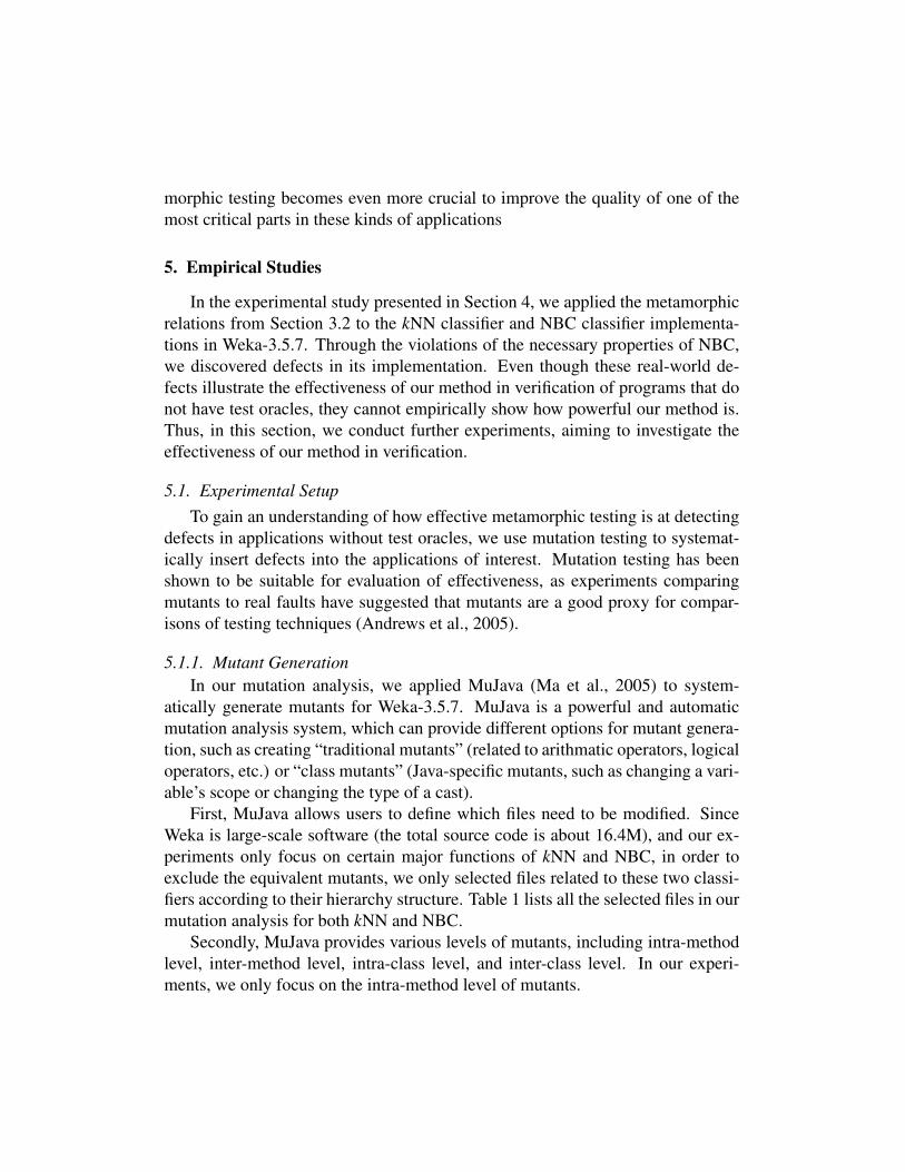
First, MuJava allows users to define which files need to be modified. SinceWeka is large-scale software (the total source code is about 16.4M), and our ex-periments only focus on certain major functions of kNN and NBC, in order toexclude the equivalent mutants, we only selected files related to these two classi-fiers according to their hierarchy structure. Table 1 lists all the selected files in ourmutation analysis for both kNN and NBC.

Secondly, MuJava provides various levels of mutants, including intra-methodlevel, inter-method level, intra-class level, and inter-class level. In our experi-ments, we only focus on the intra-method level of mutants.

kNN NBCweka.classifiers.lazy.IBk.java weka.classifiers.bayes.NaiveBayes.javaweka.core.Attribute.java weka.core.Attribute.javaweka.core.Instance.java weka.core.Instance.javaweka.core.Instances.java weka.core.Utils.javaweka.core.Utils.java weka.core.Statisticsweka.core.neighboursearch.LinearNNSearch.java weka.estimators.DiscreteEstimator.javaweka.core.neighboursearch.NearestNeighbourSearch.java weka.estimators.Estimator.javaweka.core.NormalizableDistance.java weka.estimators.KernelEstimator.javaweka.core.EuclideanDistance.java weka.estimators.NormalEstimator.java

Table 1: Selected files for mutation analysis.

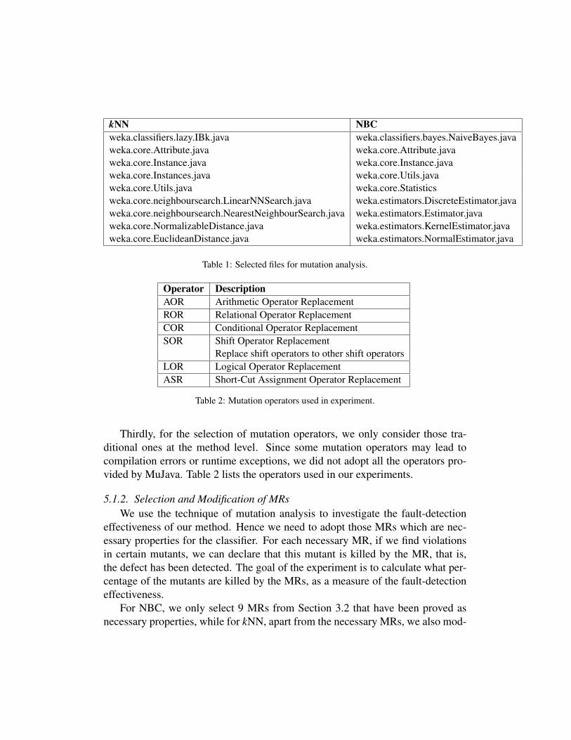
Operator DescriptionAOR Arithmetic Operator ReplacementROR Relational Operator ReplacementCOR Conditional Operator ReplacementSOR Shift Operator Replacement

Replace shift operators to other shift operatorsLOR Logical Operator ReplacementASR Short-Cut Assignment Operator Replacement

Table 2: Mutation operators used in experiment.

Thirdly, for the selection of mutation operators, we only consider those tra-ditional ones at the method level. Since some mutation operators may lead tocompilation errors or runtime exceptions, we did not adopt all the operators pro-vided by MuJava. Table 2 lists the operators used in our experiments.

5.1.2. Selection and Modification of MRsWe use the technique of mutation analysis to investigate the fault-detection

effectiveness of our method. Hence we need to adopt those MRs which are nec-essary properties for the classifier. For each necessary MR, if we find violationsin certain mutants, we can declare that this mutant is killed by the MR, that is,the defect has been detected. The goal of the experiment is to calculate what per-centage of the mutants are killed by the MRs, as a measure of the fault-detectioneffectiveness.

For NBC, we only select 9 MRs from Section 3.2 that have been proved asnecessary properties, while for kNN, apart from the necessary MRs, we also mod-

k = 1 k = 3MR-1.1 Permutation of class labels MR-0 Consistence with affine transformationMR-2.2 Addition of informative attributes MR-1.2 Permutation of the attributeMR-4.1 Addition of classes by duplicating samples MR-2.1 Addition of uninformative attributesMR-5.1 Removal of classes MR-3.1 Consistence with re-predictionMR-5.2 Removal of samples MR-3.2 Additional training sample

MR-4.2 Addition of classes by re-labeling samples

Table 3: Metamorphic relations for kNN used in mutation analysis.

MR-0 Consistence with affine transformationMR-1.1 Permutation of class labelsMR-1.2 Permutation of the attributeMR-2.1 Addition of uninformative attributesMR-2.2 Addition of informative attributesMR-3.2 Additional training sampleMR-4.1 Addition of classes by duplicating samplesMR-5.1 Removal of classesMR-NBC Consistence with value permutation

Table 4: Metamorphic relations for NBC used in mutation analysis.

ify other MRs to make them become necessary properties, to fit for our mutationanalysis. The detailed discussion of the necessity for all MRs is in the Appendix.Table 3 and Table 4 summarize the MRs used for kNN and NBC respectively inthe mutation analysis for verification.

5.2. Empirical Results and Analysis5.2.1. Metamorphic Testing Results

In the mutation analysis, we adopted 300 randomly generated inputs as sourcetest inputs. Each test input consists of one training dataset and one test case, bothof which have the same format used in the experiments described in Section 4.

In the previous experimental study, we found some real defects in the sourcecode of the NBC classifier of Weka-3.5.7. Thus in the mutation analysis, in or-der to exclude the violations that are due to these real defects, we eliminated thetest inputs which violated MRs in the original version of Weka-3.5.7. And wecheck the violated test pairs in mutants to make sure that they are really due to themodification, instead of the real defects.

Metamorphic RelationMutant 0 1.1 1.2 2.1 2.2 3.1 3.2 4.1 4.2 5.1 5.2original 0 0 0 0 0 0 0 0 0 0 0v1 0 1.67 7.67 27 5.67 0 0 0 0 6.67 3.67v2 0 0 0 0 0 0 0 0 0 4.67 3v3 0 0 0 0 42.67 0 0 0 0 4.67 3.67v5 0 2.33 0 0 0 0 0 2.33 0 6.67 3v6 0 11.33 0 26.33 37 0 0 0 0 2 0v7 0 9.67 0 0 1.67 0 0 0 0 4 1.67v9 0 9 0 0 3.33 8.33 0 41.67 0 5 2v10 0 1.33 22.67 34.33 94.67 0 0 0 0 4.33 5.33v12 0 10.33 0 0 1.67 0 0 0 0 4 1.67v13 0 0.33 22.33 0 0 0 0 0 0 3 3v15 0 0 16.33 0 13.67 0 0 0 0 3.33 2.33v16 0 10 0 26.33 37 0 0 0 0 2 0v17 0 13.67 0 0 0 0 0 0 0 0 0v18 0 11 0 0 0 0 0 0 0 0 0v19 0 9.33 0 26.33 37 0 0 0 0 2 0v20 0 0 0 0 43.67 0 0 0 0 2.33 1.67v21 0 1 0 42.67 24 0.67 0 0 0 3.67 4v22 0 68.33 0 0 0 0 0 0 0 0 0v24 0 62.67 0 0 0 0 0 0 0 0 0TOTAL 0 15 4 6 12 2 0 2 0 15 16

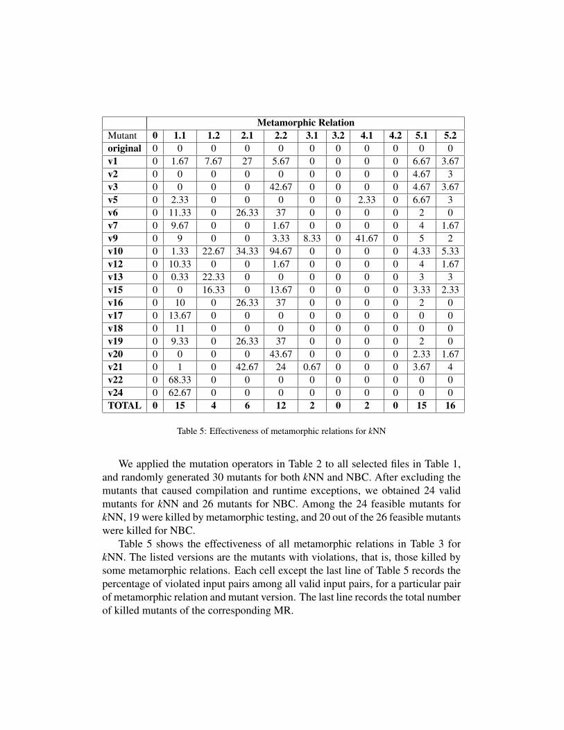
Table 5: Effectiveness of metamorphic relations for kNN

We applied the mutation operators in Table 2 to all selected files in Table 1,and randomly generated 30 mutants for both kNN and NBC. After excluding themutants that caused compilation and runtime exceptions, we obtained 24 validmutants for kNN and 26 mutants for NBC. Among the 24 feasible mutants forkNN, 19 were killed by metamorphic testing, and 20 out of the 26 feasible mutantswere killed for NBC.

Table 5 shows the effectiveness of all metamorphic relations in Table 3 forkNN. The listed versions are the mutants with violations, that is, those killed bysome metamorphic relations. Each cell except the last line of Table 5 records thepercentage of violated input pairs among all valid input pairs, for a particular pairof metamorphic relation and mutant version. The last line records the total numberof killed mutants of the corresponding MR.

It can be seen from Table 5 that our method is very effective in killing mu-tants: 19 out of 24 mutants have been killed by the current source inputs andall 11 metamorphic relations. After examining the five surviving mutants, wediscovered that three out of the five mutants are equivalent mutants with respectto the current source inputs, the parameters in the command line, and all the 11metamorphic relations. The reason for the equivalent mutants is that Weka is alarge-scale program; even though we have selected the related program files formutation analysis, we do not target all the functionality in these files. The param-eters we used in the command line and the metamorphic relations that we haveenumerated are only targeted for certain properties of the program. Thus in thethree mutants, the modified statements are not executed using the current sourceinputs, the parameters in command line, and all the 11 metamorphic relations.Hence the actual effectiveness is 90.5%(19 out of 21 mutants).

The results in Table 5 also show that different metamorphic relations havedifferent performance in detecting program faults. Among all 11 MRs, MR-1.1and MR-5.1 had the highest killing rate (15 out of 21, 71.4%), while MR-0, MR-3.2 and MR-4.2 had the lowest killing rate (0 out of 21).

We also investigated the average violation percentage of all MRs. Since weenumerated all the metamorphic relations only by means of the background knowl-edge of the classifier without referring to the source code of the Weka implemen-tation, and we also generated all mutants and test inputs randomly, our metamor-phic relations are hence unbiased to any mutants under investigation. In this way,the average violation percentage for the MRs over all mutants (including all thesurvived mutants) can be used as an effectiveness measurement of metamorphictesting, that is, how likely a test input pair (source test input and follow-up testinput) on average will reveal a violation. From Table 5, we can calculate that forkNN, the average percentage is 3.65% for all the mutants in table.

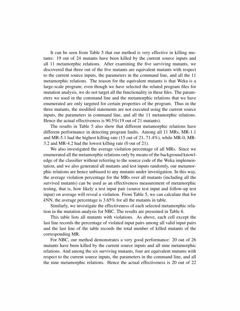
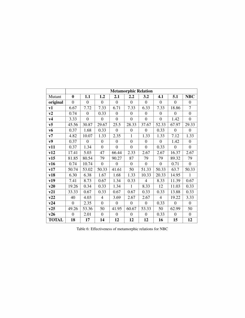
Similarly, we investigate the effectiveness of each selected metamorphic rela-tion in the mutation analysis for NBC. The results are presented in Table 6.

This table lists all mutants with violations. As above, each cell except thelast line records the percentage of violated input pairs among all valid input pairsand the last line of the table records the total number of killed mutants of thecorresponding MR.

For NBC, our method demonstrates a very good performance: 20 out of 26mutants have been killed by the current source inputs and all nine metamorphicrelations. And among the six surviving mutants, four are equivalent mutants withrespect to the current source inputs, the parameters in the command line, and allthe nine metamorphic relations. Hence the actual effectiveness is 20 out of 22

Metamorphic RelationMutant 0 1.1 1.2 2.1 2.2 3.2 4.1 5.1 NBCoriginal 0 0 0 0 0 0 0 0 0v1 6.67 7.72 7.33 6.71 7.33 6.33 7.33 18.86 7v2 0.74 0 0.33 0 0 0 0 0 0v4 3.33 0 0 0 0 0 0 1.42 0v5 45.56 30.87 29.67 25.5 28.33 37.67 52.33 67.97 29.33v6 0.37 1.68 0.33 0 0 0 0.33 0 0v7 4.82 10.07 1.33 2.35 1 1.33 1.33 7.12 1.33v9 0.37 0 0 0 0 0 0 1.42 0v11 0.37 1.34 0 0 0 0 0.33 0 0v12 17.41 5.03 47 66.44 2.33 2.67 2.67 16.37 2.67v15 81.85 80.54 79 90.27 87 79 79 89.32 79v16 0.74 10.74 0 0 0 0 0 0.71 0v17 50.74 53.02 50.33 41.61 50 51.33 50.33 63.7 50.33v18 6.30 6.38 1.67 1.68 1.33 10.33 20.33 14.95 1v19 7.41 8.73 0.67 1.34 0.33 4 8.33 11.39 0.67v20 19.26 0.34 0.33 1.34 1 8.33 12 11.03 0.33v21 33.33 0.67 0.33 0.67 0.67 0.33 0.33 13.88 0.33v22 40 4.03 4 3.69 2.67 2.67 4 19.22 3.33v24 0 2.35 0 0 0 0 0.33 0 0v25 49.26 53.36 50 41.95 60.67 53.33 50 62.99 50v26 0 2.01 0 0 0 0 0.33 0 0TOTAL 18 17 14 12 12 12 16 15 12

Table 6: Effectiveness of metamorphic relations for NBC

mutants (90.9%).Different from kNN, where some MRs kill none or a small number of mutants,

in NBC, close to 50% of the mutants are killed by any given MR. For example,MR-0, which kills no mutants in kNN, can kill 18 mutants in NBC. And conse-quently the average violation percentage of the nine MRs over all the mutants intable is much higher than that in kNN. The average effectiveness of metamorphictesting for NBC is 11.19%.

5.2.2. Cross-validation AnalysisApart from metamorphic testing, we also conducted cross-validation on these

mutants. In the machine learning community, cross-validation is commonly usedto assess how well the classification algorithms can model the classification pro-cess. In the context of applying cross-validation, it is often implicitly assumedthat the implementation of the algorithm is correct. The focus is on the appropri-ateness of the classification algorithm to the given problem. While in our study,since we have investigated the well-known classification algorithms, we assumethat they should perform well in cross-validation with reasonable datasets. Ourmajor concern is whether the implementation of these algorithms is correct.

For most commonly used classification algorithms, a correct implementationfor these algorithms should give a good cross-validation result when we use a rea-sonable dataset that contains discriminatory signals among samples of differentclasses; while an implementation with bad cross-validation performance justifiesa further investigation which may lead to identification of software faults. How-ever, in our experiments, we discovered that quite a few mutants can survive thecross-validation procedure, that is, the program that actually contains faults canstill perform very well in cross-validation. As a consequence, this observation im-plies that proper software testing, particularly using the metamorphic testing tech-nique proposed in this paper, is indispensable for these kind of machine learningapplications.

In our experiments, we conducted k-fold cross-validation, which is a typicalcross-validation method. In k-fold cross-validation, the original sample set is ran-domly partitioned into k subsets. Among the k subsets, a single subset is retainedas the validation data for testing the classifier model, and the remaining (k ≤ 1)subsets are used as training data. The cross-validation process is then repeatedk times. The k results from the k folds then can be averaged or summarized (orotherwise combined) to produce a single estimation (McLachlan et al., 2004). Incross-validation, a classifier is simply evaluated in terms of its respective frac-tion of misclassified instances, noted as the error-rate. A lower error-rate means

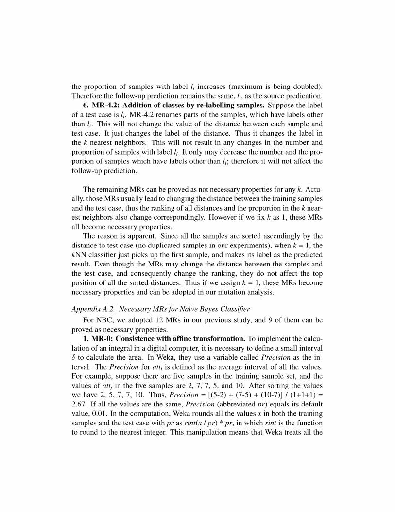
a better performance of a classifier. Usually an error-rate lower than 30% can beregarded as a reasonable one in a two-class classification problem.

We used some simulation data for our cross-validation analysis. The simulateddatasets that we adopted have similar sizes and formats as the randomly generateddata used in the mutation analysis. They were produced and used in another bioin-formatics study (Ho et al., 2008) that simulates microarray gene expression datacontaining realistic noise characteristics. Each simulated dataset contains five nu-meric attributes and 100 samples comprising five classes of 20 samples each. Theexpression level of each attribute is simulated with a normal distribution N(µ, σ2).The same value is used for variance (σ2 = 2) in all simulated datasets, and µ varieswith three different rules, referred as Rule-1, Rule-1.5 and Rule-2 respectively inthe paper. Each rule is to multiply the data in consecutive classes with a normaldistribution with the same σ2 and different µ*γ where γ is a multiplication factoraccording to the current rule. The value of γ is assigned as 1, 1.5 and 2 in corre-sponding rules, in order to approximate the effect of observing no, medium, andlarge signals for distinguishing among different classes. We utilize 300 datasets ofeach rule, hence have a total of 900 datasets for the cross-validation experiment.

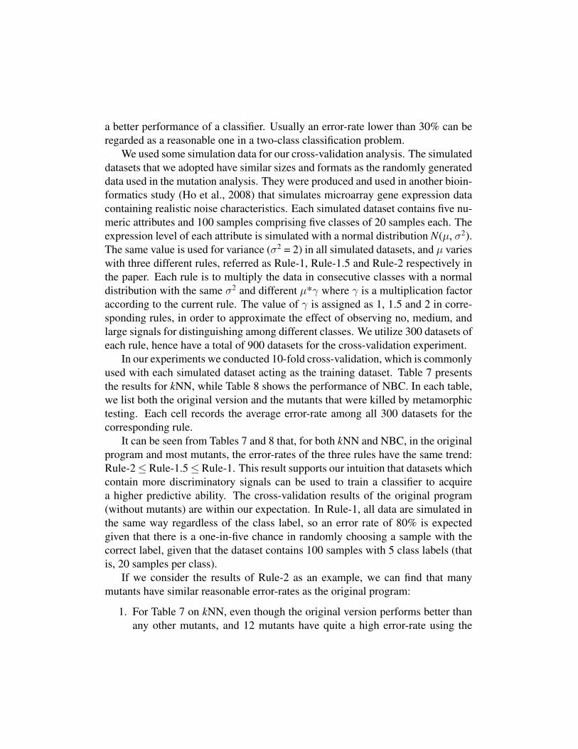
In our experiments we conducted 10-fold cross-validation, which is commonlyused with each simulated dataset acting as the training dataset. Table 7 presentsthe results for kNN, while Table 8 shows the performance of NBC. In each table,we list both the original version and the mutants that were killed by metamorphictesting. Each cell records the average error-rate among all 300 datasets for thecorresponding rule.

It can be seen from Tables 7 and 8 that, for both kNN and NBC, in the originalprogram and most mutants, the error-rates of the three rules have the same trend:Rule-2≤ Rule-1.5≤ Rule-1. This result supports our intuition that datasets whichcontain more discriminatory signals can be used to train a classifier to acquirea higher predictive ability. The cross-validation results of the original program(without mutants) are within our expectation. In Rule-1, all data are simulated inthe same way regardless of the class label, so an error rate of 80% is expectedgiven that there is a one-in-five chance in randomly choosing a sample with thecorrect label, given that the dataset contains 100 samples with 5 class labels (thatis, 20 samples per class).

If we consider the results of Rule-2 as an example, we can find that manymutants have similar reasonable error-rates as the original program:

1. For Table 7 on kNN, even though the original version performs better thanany other mutants, and 12 mutants have quite a high error-rate using the

Mutants Rule-1 Rule-1.5 Rule-2original 80.07 3.95 0.06v1 79.78 10.58 1.55v2 80.07 3.95 0.06v3 79.97 80 80v5 80.05 6.75 0.15v6 80 80 80v7 79.72 5.79 1.23v9 80.04 44.4 40.84v10 80.09 100 100v12 79.72 5.79 1.23v13 80.07 5.66 0.21v15 80.12 100 100v16 80 80 80v17 80 80 80v18 80 80 80v19 80 80 80v20 80.18 80 80v21 79.91 80 80v22 100 100 100v24 100 100 100

Table 7: Cross-validation error rate for kNN.

Mutants Rule-1 Rule-1.5 Rule-2original 80.07 3.36 0.07v1 80.61 49.68 60v2 79.97 3.35 0.07v4 80.19 3.43 0.09v5 80 80 80v6 79.97 3.36 0.07v7 80 80 80v9 80 3.34 0.08v11 79.97 3.36 0.07v12 80.18 18.20 3.49v15 100 100 100v16 80 80 80v17 80.21 81.09 91.2v18 80 80 80v19 80 80 80v20 79.90 27.24 39.89v21 80 80 5.35v22 80 80 60v24 79.95 3.37 0.07v25 80.19 81.05 91.04v26 79.97 3.36 0.07

Table 8: Cross-validation error rate for NBC.

dataset of Rule-2, there are still six mutants having an error-rate close to1%, and one mutant that has an error rate of 40%, using the same dataset.

2. Table 8 shows that performance for mutants is even better in NBC. In NBC,the original version is no longer the only one having the lowest error-rate;there are five mutants that have the same error-rate (0.07%). Actually halfof the mutants acquire quite good classification performance (error rate lessthan 5.5%), and one mutant has a reasonable error-rate (39.89%).

These experimental data reveal that some mutants can achieve relatively good per-formances in cross-validation, despite the fact that these mutants are faulty imple-mentations of the algorithms. Actually cross-validation has been widely adoptedas the main method for evaluating a supervised classifier system for decades; how-ever, it was never designed for the purpose of either verification or validation. But,most practitioners in the machine learning field have relied on the cross-validationmethod to check the correctness of the implementation of the algorithm. In otherwords, an additional way to verify the correctness of the implementation is nec-essary. Because of the oracle problem, metamorphic testing becomes necessaryand suitable in testing these supervised machine learning programs. In fact, meta-morphic testing is very powerful in detecting faults even for mutants with verylow error-rate. For example, v1 of kNN has an ASR mutant in the EuclideanDis-tance.java file, line 182. The modification is:

result = diff * diff; //correct: result += diff * diff;However in Table 7, v1 for Rule-2 has the error-rate as low as 1.55%. Fortu-

nately metamorphic testing is able to kill this mutant. Table 5 shows that MR-1.1,MR-1.2, MR-2.1, MR-2.2, MR-5.1 and MR-5.2 all reveal this mutant.

This result shows that the cross-validation technique is not sufficient to test thecorrectness of a supervised classification program. It is strongly recommended toadopt MT as the complement to this technique in order to provide more confidenceof the software quality.

6. Related Work

Although there has been much work that applies machine learning techniquesto software engineering in general and software testing in particular (e.g., Briand(2008)), we are not currently aware of any other work in the reverse sense: apply-ing software testing techniques to machine learning applications. ML frameworkssuch as Orange (Demsar et al., 2004) provide testing functionality but it is focusedon comparing the quality of the results, and not evaluating the “correctness” of the

implementations. Repositories of “reusable” data sets have been collected (e.g.,Newman et al. (1998)) for the purpose of comparing result quality, that is, howaccurately the algorithms predict, but not for the software engineering sense oftesting (to reveal defects).

Applying metamorphic testing to situations in which there is no test oraclewas first suggested in Chen et al. (1998) and is further discussed in Chen et al.(2002). Metamorphic testing has previously been shown to be effective in testingdifferent types of machine learning applications (Murphy et al., 2008), and hasrecently been applied to testing specific scientific computation applications, suchas in bioinformatics (Chen et al., 2009). The work we present here seeks to extendthe previous techniques to scientific computation domains that rely on machinelearning.

7. Conclusion

As noted in Kelly and Sanders (2008), “scientists want to do science” and donot want to spend time addressing the challenges of software development. Thus,it falls upon the software engineering community to develop simple yet powerfulmethods to perform testing and validation. Our contribution is a set of metamor-phic relations for classification algorithms, as well as a technique that uses theserelations to enable scientists to easily test and validate the machine learning com-ponents of their software; this technique is also applicable to problem-specificdomains as well. We hope that our work helps to improve the quality of the soft-ware being developed in the fields of computational science and engineering.

Acknowledgments

This project is partially supported by an Australian Research Council Discov-ery Grant (ARC DP0771733), as well as the National Natural Science Foundationof China (90818027 and 60721002), the National High Technology DevelopmentProgram of China (2009AA01Z147), and the Major State Basic Research Devel-opment Program of China (2009CB320703). Ho is supported by an AustralianPostgraduate Award and a NICTA Research Project Award. Murphy and Kaiserare members of the Programming Systems Laboratory, funded in part by CNS-0905246, CNS-0717544, CNS-0627473, CNS-0426623 and EIA-0202063, andNIH grant 1U54CA121852-01A1.

Reference

Andrews, J. H., Briand, L. C., Labiche, Y., 2005. Is mutation an appropriate toolfor testing experiments? In: Proc. of the 27th International Conference on Soft-ware Engineering (ICSE). pp. 402–411.

Briand, L., 2008. Novel applications of machine learning in software testing. In:Proc. of the 8th International Conference on Quality Software(QSIC). pp. 3–10.

Chen, T. Y., Cheung, S. C., Yiu, S., 1998. Metamorphic testing: a new approachfor generating next test cases. Tech. Rep. HKUST-CS98-01, Dept. of ComputerScience, Hong Kong Univ. of Science and Technology.

Chen, T. Y., Ho, J. W. K., Liu, H., Xie, X., 2009. An innovative approach for test-ing bioinformatics programs using metamorphic testing. BMC Bioinformatics10, 24–36.

Chen, T. Y., Huang, D. H., Tse, T. H., Zhou, Z. Q., 2004. Case studies on theselection of useful relations in metamorphic testing. In: Proc. of the 4th Ibero-American Symposium on Software Engineering and Knowledge Engineering(JIISIC 2004). pp. 569–583.

Chen, T. Y., Tse, T. H., Zhou, Z. Q., 2002. Fault-based testing without the need oforacles. Information and Software Technology 44 (15), 923–931.

Davis, M. D., Weyuker, E. J., 1981. Pseudo-oracles for non-testable programs. In:Proc. of the ACM Annual Conference. pp. 254–257.

Demsar, J., Zupan, B., Leban, G., Curk, T., 2004. Orange: From experimental ma-chine learning to interactive data mining. Lecture Notes in Computer Science,537–539.

Duran, J., Ntafos, S., 1984. An evaluation of random testing. IEEE Transactionson Software Engineering 10, 438–444.

Gewehr, J. E., Szugat, M., Zimmer, R., 2007. BioWeka - extending the Wekaframework for bioinformatics. Bioinformatics 23 (5), 651–653.

Ho, J. W. K., Lin, M. W., Adelstein, S., dos Remedios, C. G., 2010. Customisingan antibody leukocyte capture microarray for systemic lupus erythematosus:Beyond biomarker discovery. Proteomics - Clinical Applications in press.

Ho, J. W. K., Stefani, M., dos Remedios, C. G., Charleston, M. A., 2008. Dif-ferential variability analysis of gene expression and its application to humandiseases. Bioinformatics 24, 390–398.

Kelly, D., Sanders, R., 2008. Assessing the quality of scientific software. In: Proc.of the 1st International Workshop on Software Engineering for ComputationalScience and Engineering(SECSE).

Knight, J., Leveson, N., 1986. An experimental evaluation of the assumption ofindependence in multi-version programming. IEEE Transactions on SoftwareEngineering 12 (1), 96–109.

Ma, Y.-S., Offutt, J., Kwon, Y. R., June 2005. MuJava: An automated class mu-tation system. Journal of Software Testing, Verification and Reliability 15 (2),97–133.

Manning, C. D., Schutze, H., 1999. Foundations of Statistical Natural LanguageProcessing. The MIT Press.

McLachlan, G. J., Do, K.-A., Ambroise, C., 2004. Analyzing microarray geneexpression data. Wiley.

Middendorf, M., Kundaje, A., Shah, M., Freund, Y., Wiggins, C. H., Leslie,C., 2005. Motif discovery through predictive modeling of gene regulation. Re-search in Computational Molecular Biology 3500, 538–552.

Mitchell, T., 1983. Machine Learning: An Artificial Intelligence Approach, Vol.III. Morgan Kaufmann.

Murphy, C., Kaiser, G., Hu, L., Wu, L., 2008. Properties of machine learningapplications for use in metamorphic testing. In: Proc. of the 20th InternationalConference on Software Engineering and Knowledge Engineering (SEKE). pp.867–872.

Newman, D. J., Hettich, S., Blake, C. L., Merz, C. J., 1998. UCI repository ofmachine learning databases. University of California, Dept of Information andComputer Science.

SVM Application List, 2006. http://www.clopinet.com/isabelle/Projects/SVM/applist.html.

Weyuker, E. J., November 1982. On testing non-testable programs. ComputerJournal 25 (4), 465–470.

Witten, I. H., Frank, E., 2005. Data Mining: Practical Machine Learning Toolsand Techniques, 2nd Edition. Morgan Kaufmann.

Xie, X. Y., Ho, J. W. K., Murphy, C., Kaiser, G., Xu, B. W., Chen, T. Y., 2009.Application of metamorphic testing to supervised classifiers. In: Proc. of the9th International Conference on Quality Software(QSIC). pp. 135–144.

Appendix A.

In the appendix, we discuss the necessity of MRs for both kNN and NBC.

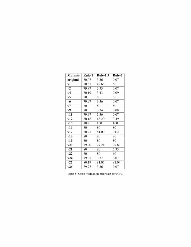
Appendix A.1. Necessary MRs for k-Nearest NeighborsIn our previous study (Xie et al., 2009), we adopted a total of 11 MRs on kNN,

and 6 of them can be proved as necessary properties for kNN with any value of k.1. MR-0: Consistence with affine transformation.

Each value in the training sample set and in the test case is transformed in thisway: kx+b (k 6= 0). Thus, this MR does not change the distance between si and ts.The distance is:

dist(si’, ts’) =

√√√√ m∑j

[(k ∗ saj + b)− (k ∗ aj + b)]2 = k

√√√√ m∑j

(saj − aj)2.

Therefore MR-0 does not change the order in the k nearest neighbors and willstill give the same prediction.

2. MR-1.2: Permutation of the attribute. It can be seen from the formula forcalculating the distance that the result is not related to the order of the attributes.Thus, the permutation of the attributes will not affect the prediction result.

3. MR-2.1: Addition of uninformative features. In this MR, we add a newattribute attm to both the samples and the test case and assign them with the samevalue. Suppose the value of attm is a. It is obvious that MR-2.1 will not changethe distance between any sample si and test case ts. The new distance is:

dist(si’, ts’) =

√√√√m−1∑j

(saj − aj)2 + (a− a)2 =

√√√√m−1∑j

(saj − aj)2.

Therefore MR-2.1 does not change anything in the k nearest neighbors andwill still give the same prediction.

4. MR-3.1: Consistence with re-prediction. Suppose the label of a test caseis li. We put the test case back into the training sample set, and from the distanceformula we can know that the distance between the new sample and the test case is0. Thus, the number of samples with label li in the k nearest neighbors increases by1, and obviously the proportion of samples with label li will increases. Therefore,the follow-up prediction remains the same, li, as the source prediction.

5. MR-3.2: Additional training sample. Suppose the label of a test case is li.MR-3.2 duplicates the samples with label li in the training sample set. These newsamples have the same value as the old ones, thus the number of samples with labelli increases in the k nearest neighbors (maximum is being doubled). Meanwhile,the samples with other labels are excluded from the k nearest neighbors. Thus,

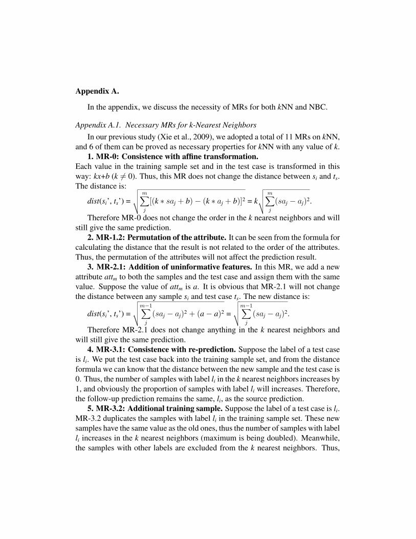
the proportion of samples with label li increases (maximum is being doubled).Therefore the follow-up prediction remains the same, li, as the source predication.

6. MR-4.2: Addition of classes by re-labelling samples. Suppose the labelof a test case is li. MR-4.2 renames parts of the samples, which have labels otherthan li. This will not change the value of the distance between each sample andtest case. It just changes the label of the distance. Thus it changes the label inthe k nearest neighbors. This will not result in any changes in the number andproportion of samples with label li. It only may decrease the number and the pro-portion of samples which have labels other than li; therefore it will not affect thefollow-up prediction.

The remaining MRs can be proved as not necessary properties for any k. Actu-ally, those MRs usually lead to changing the distance between the training samplesand the test case, thus the ranking of all distances and the proportion in the k near-est neighbors also change correspondingly. However if we fix k as 1, these MRsall become necessary properties.

The reason is apparent. Since all the samples are sorted ascendingly by thedistance to test case (no duplicated samples in our experiments), when k = 1, thekNN classifier just picks up the first sample, and makes its label as the predictedresult. Even though the MRs may change the distance between the samples andthe test case, and consequently change the ranking, they do not affect the topposition of all the sorted distances. Thus if we assign k = 1, these MRs becomenecessary properties and can be adopted in our mutation analysis.

Appendix A.2. Necessary MRs for Naıve Bayes ClassifierFor NBC, we adopted 12 MRs in our previous study, and 9 of them can be

proved as necessary properties.1. MR-0: Consistence with affine transformation. To implement the calcu-

lation of an integral in a digital computer, it is necessary to define a small intervalδ to calculate the area. In Weka, they use a variable called Precision as the in-terval. The Precision for attj is defined as the average interval of all the values.For example, suppose there are five samples in the training sample set, and thevalues of attj in the five samples are 2, 7, 7, 5, and 10. After sorting the valueswe have 2, 5, 7, 7, 10. Thus, Precision = [(5-2) + (7-5) + (10-7)] / (1+1+1) =2.67. If all the values are the same, Precision (abbreviated pr) equals its defaultvalue, 0.01. In the computation, Weka rounds all the values x in both the trainingsamples and the test case with pr as rint(x / pr) * pr, in which rint is the functionto round to the nearest integer. This manipulation means that Weka treats all the

values within ((2k-1)* pr/2, (2k+1)* pr/2] as k*pr, in which k is any integer. Thismanipulation may lead to a loss of precision; however, it provides a mechanism todisperse the continuous values in the mathematic model, in order to be make themodel suitable for computer implementation.

In Weka, the small interval δ is the magnitude of precision. According toformula for calculating area, we have:

P(aj | lts = lk) = 1σ√

2π

∫ aj+pr/2

aj−pr/2e-(x - µ)2 / 2σ2

dx.

In MR-0, each value x in the training set and the test case are transformed inthis way: ϕ = k*x+b (k 6= 0). According to the calculation of pr, pr’ is set to bek*pr + b. According to the formula of mean value µ and mean square deviation σ,we have µ’ = k*µ + b, and σ’ = k*σ. And the formula for probability is as follows:

P(k * aj + b | lts = lk) = 1σ′√

2π

∫ k∗aj+b+k∗pr/2

k∗aj+b−k∗pr/2e-(ϕ - µ’)2 / 2σ′2 dϕ

by substituting σ′ with k ∗ σ, and µ′ with k ∗ µ+ b, we have:

P(k * aj + b | lts = lk) = 1kσ√2π

∫ k∗aj+b+k∗pr/2

k∗aj+b−k∗pr/2e-(ϕ - kµ - b)2 / 2kσ2

dϕ

by substituting ϕ with k ∗ x+ b, we have:

P(k * aj + b | lts = lk) = 1kσ√2π

∫ aj+pr/2

aj−pr/2e-(kx + b - kµ - b)2 / 2k2σ2

d(kx + b)

=⇒ P(k * aj + b | lts = lk) = 1σ√

2π

∫ aj+pr/2

aj−pr/2e-(x - µ)2 / 2σ2

dx = P (aj | lts = lk).

It can be seen from the above formula that after the transformation, the prob-ability will not change, thus the prediction result will not change either.

2. MR-1.1: Permutation of class labels. This MR reflects a key property ofmathematical function such as NBC that the output of the classifier is determinis-tic, and is not affected by random permutation.

3. MR-1.2: Permutation of the attribute. It is known that in NBC, weassume all the attributes are independent, thus we have the following formula:

P(lts = lk | a0a1...am-1) =

P(lk)∏j

P(aj | lts = lk)∑iP(li)

∏jP(aj|lts = li)

Therefore, changing the attribute order will not affect the prediction result.Actually, it can be concluded that all classifiers should have a consistent result

in this MR, assuming the attributes are independent to each other.4. MR-2.1: Addition of uninformative features. In this MR, we add a new

attribute attm with identical value to both the samples and the test case. Suppose

the value of attm is a. For each lk ∈ {l0, l1, ..., ln-1}, the probability P(lts = lk |a0a1...am-1) can be re-written in the following way:

P(lts = lk | a0a1...am) =

P(lts = lk)∏j

P(aj | lts = lk) ∗ P(attm = a | lts = lk)∑iP(lts=li)

∏jP(aj|lts = li)∗P(attm=am|lts=li)

Since the new attribute attm has the same value a in all the samples, the meanvalue µ = a and the mean square deviation σ = 0. Thus the P(attm = a | lts = lk)part is equal to 1 for all the lk ∈ {l0, l1, ..., ln-1}.

In Weka, since it is infeasible for computer to deal with the normal distributionwith σ = 0, they give σ a default minimum of pr/2*3. Thus for each lk ∈ {l0, l1,..., ln-1}, the numerator in the formula above will be changed by multiplying aconstant value P(attm = a | lts = lk), which is a little less than 1.

It follows that the probability for each lk ∈ {l0, l1, ..., ln-1} changes in thesame way. Thus the order of the probabilities will not change; consequently theprediction in the follow-up cases will remain the same as the one in the sourcecases.

5. MR-2.2: Addition of informative features. In this MR, we add a newattribute attm to both the samples and the test case and assign the samples havingthe same label with the same value; meanwhile, we assign the new attribute’svalue in the test case as the one of its predicted label. For example, suppose thereare three classes in the training samples, {l0, l1, l2}, and the predicted label of thetest case is l0. In the MR-2.2 transformation, we add a new attribute and makeit different among different classes, that is, for samples with l0, the attm = a; forsamples with l1, the attm = b; for samples with l2, the attm = c; and for the testcase, the attm = a.

Since the denominator in the formula for each lk ∈ {l0, l1, ..., ln-1} are the same,only the numerator will affect the result.

For l0, the mean value of attm is µ = a; the mean square deviation of attm is σ= δ (since it is hard to deal with a normal distribution with σ = 0, we assign a verysmall number to σ).

For l1, the mean value of attm is µ = b; the mean square deviation of attm is σ= δ.

For l2, the mean value of attm is µ = c; the mean square deviation of attm is σ= δ.

Thus the numerator in the formula for l0 is multiplied by a value of P(attm =a | lts = l0), which is quite close to 1. Also, the numerator in the formula for l1 ismultiplied by a value of P(attm = b | lts = l1), which is quite close to 0. Last, thenumerator in the formula for l2 is multiplied by a value of P(attm = c | lts = l2),

which is quite close to 0.Therefore the former highest possibility almost remains the same, while the

other two decrease dramatically. Consequently the follow-up prediction will re-main the same as in the source case.

6. MR-3.2: Additional training sample. Suppose the label of test case isli. MR-3.2 duplicates the samples with label li in the training data set. Those newsamples have the same value as the old ones, thus the mean value and the meansquare deviation of each attribute in li will not change. Meanwhile, the meansquare deviation of each attribute in other labels will not change either. The onlychange is the proportion of each lk ∈ {l0, l1, ..., ln-1}: P(lts = lk); that is, P(lts = li)increases, while P(lts = lk) for the other labels decreases.

Therefore the probability of ts belonging to li increases, while the probabilityof ts being one of the other labels decreases. The prediction is still li, as in thesource case.

7. MR-4.1: Addition of classes by duplicating samples. Suppose we havelabels {l0, l1, ..., ln-1}, the number of each distinct label li ∈ {l0, l1, ..., ln-1} in thetraining sample set is count[i], and its corresponding proportion is proportion[i].For each li ∈ {l0, l1, ..., ln-1}, the mean value of attj is µij; the mean square de-viation is σij. Suppose the prediction in source case is lk. Thus in the MR-4.1transformation, we duplicate all samples with li ∈ {l0, l1, ..., ln-1} (i 6= k) and re-name them as li’. After duplication the µij and σij for the original labels remainthe same value as the ones in the source case. The only change is the proportion[],which is as follows:

proportion’[i] = proportion[i] *

m−1∑0

count[i]

count[0]+2∑m−1

1count[i]

And for the new added label li’, their µ, σ and proportion[] values are all thesame for li. Therefore proportion[0] remains the highest value, and the predictionwill not change in the follow-up case.

8. MR-5.1: Removal of classes. This MR transformation only changes theproportion of each class, rather than changing the distribution in each survivedclass. Suppose we have labels {l0, l1, ..., ln-1}, the number of each distinct labelli ∈ {l0, l1, ..., ln-1} in the training sample set is count[i], and its correspondingproportion is proportion[i]. For each li ∈ {l0, l1, ..., ln-1}, the mean value of attj isµij; the mean square deviation is σij. Suppose the prediction in the source case isl0, and l2 is the label being removed. Thus, after transformation, the µ and σ foreach survived label remain the same as in the source case. The only change is thecount[i] and the proportion[i], which changes as follows:

proportion’[i] = proportion[i] *

m−1∑0

count[i]∑m−1

0count[i]−count[2]

Therefore, the prediction remains the same as in the source case.9. MR-NBC: Consistence with value permutation. NBC assumes that all

the attributes are independent. If we permute the value of attrj among all sampleswith label li, this will not change the P(attrj | lts = li). Because for each li ∈ {l0,l1, ..., ln-1}, the mean value µij of attj, and the mean square deviation σij will notchange in this permutation. Thus MR-NBC will not change the prediction madein the source case.