Programs for Tree Classifiers

An early program for classification and regression trees was called

CART by Breiman, Friedman, Olshen and Stone.

They trademarked the name CART.

Clark and Pregibon wrote a classification and regression tree

program for S called tree.

With modifications, it is the program in the R package tree.

Therneau and Atkinson wrote a classification and regression tree

program for R called rtree.

It has more options.

1

Optional Parameters in rtree

method one of ”anova”, ”poisson”, ”class” or ”exp”.

If method is missing then the routine tries to make an intelligent

guess.

It is wisest to specify the method directly, especially as more

criteria may added to the function in future.

parms optional parameters for the splitting function.

control a list of options that control details of the rpart algo-

rithm. More description is in rpart.control.

cost a vector of non-negative costs, one for each variable in the

model. Defaults to one for all variables. These are scalings to be

applied when considering splits, so the improvement on splitting

on a variable is divided by its cost in deciding which split to

choose.

2

Classification of Vowel Data Using Defaults of

rpart

library(rpart)

vfitr <- rpart(as.factor(y)~x.1+x.2+x.3+x.4+x.5+x.6+x.7+x.8+x.9+x.10,dat

plot(vfitr)

text(vfitr,cex=0.5)

vtrainpr <- predict(vfitr,vtrain,type="class")

sum(vtrainpr!=vtrain[,2])/dim(vtrain)[1]

vtestpr <- predict(vfitr,vtest,type="class")

sum(vtestpr!=vtest[,2])/dim(vtest)[1]

Missclassification on training data: 0.1628788

Missclassification on test data: 0.5627706

3

Classification Trees

If we assume that a classification tree is built from observations

on random variables, then the classification tree is a random

variable.

It is a statistic. (definition)

What do we want to know about statistics (that is, about things

we use as estimators, tests, classifiers, etc.)?

Biased?

Variance?

Maximum likelihood?

etc.

4

Properties of Statistics

They generally depend on some underlying probability model.

Generally in statistical learning, we avoid assumptions about

probability models.

Nevertheless, we can ask about the variance of a tree.

How?

Vary the input data and observe how much the results vary.

By this type of assessment, classification trees have high vari-

ance.

5

Properties of Statistics

Another thing we ask about statistical procedures is how resistant

they are to real-world-type problems in the input data.

Outliers (in feature space)? Actually, trees don’t do so badly.

Outliers in the response (misclassification in the training data)?

What can I say? It’s a problem.

Missing data? If the response variable is missing, the observation

must be thrown out.

If a feature variable is missing, however, what can we do?

Throw out.

Impute the value.

Use as much of the data as possible.

6

Ensemble Methods

Ensemble methods involve decisions based on more than one

fitted model.

In classification, for example, we may wish to classify an object

based on an observed feature vector x.

Suppose we have built various classifiers from our training data,

C1, C2, . . . Cm.

The jth classifier yields Cj(x).

Suppose the classifiers do not all yield the same class. Which do

we choose?

We may take a majority vote, or we may use some other method

of combining the different decisions into a single one.

The variability in the results provides some insight about the

confidence we can place in our decision.

7

Bootstrapping

Alternative results give us better understanding of the statisti-

cal methods we use, and also some indication of the underlying

variability in the data.

One way of getting alternative results even from a single statis-

tical method is to use bootstrap resampling.

Given a sample, X1, . . . , Xn, we can envision an underlying prob-

ability model in which a random variable takes on the any exact

value X1, . . . , Xn with probability 1/n.

Instead of trying to use an unknown underlying probability dis-

tribution for data-generating process, we’ll use this uniform dis-

tribution that statistically approximates it.

8

Bootstrapping

How could we learn more about this distribution?

This distribution is pretty simple, but what we’re really inter-

ested in is how some particular statistical method works in this

distribution.

How could be study the performance of our statistical method?

Draw random samples from the uniform distribution, and apply

the statistical method to each one.

Let X∗j1 , . . . , X

∗jn represent the jth random sample from the dis-

crete uniform distribution with mass points X1, . . . , Xn.

We’ll take m such random samples, and apply our statistical

method to each.

These are called bootstrap samples.

9

Bootstrapping

Notice that each element of the bootstrap sample X∗ji is equal

to some value in the original sample X1, . . . , Xn.

For this reason, the bootstrap process is sometimes called “re-

sampling”.

Operationally, it can be viewed as sampling with replacement

from the population X1, . . . , Xn.

10

Bootstrapping in Classification Trees

In a classification problem, we have the data (Y1, X1), . . . , (Yn, Xn).

A bootstrap sample would be (Y, X)∗j1 , . . . , (Y, X)

∗jn . (Note that

the pairs are preserved.)

The bootstrap sample would probably not include every observa-

tion from the original dataset, and it would probably include the

same observation more than once. (What about the probabilities

here?)

We can apply the same classification method to each bootstrap

sample that we used on the original problem.

We get the classifiers C∗1, C∗2, . . . C∗m.

11

Bagging

Bootstrapping and aggregating the results is called “bagging”.

In classification trees, the classifiers are based on the same pre-

dictors.

An important property of bootstrapped classification trees is

that an estimate of the misclassification error can be obtained

from the training sample by passing all “out-of-bag” observations

through all of the m classifiers C∗j and averaging.

Of course, there is strong correlation among the C∗1, C∗2, . . . C∗m

because they are built from the same set of features.

12

Random Feature Selection

The idea of subsampling can also be applied to the features.

(Bootstrapping them would not make sense. Why?)

Each set of features yields a classifier.

This is particularly useful if the number of features is large, the

n � p problem, or if they are strongly correlated.

This kind of ensemble method is handled in the same kind of

ways as any other.

13

Random Forests

Random forests is a bootstrapping method applied to classifica-

tion trees with a random selection of features in the formation

of each node. It was originally developed by Breiman (2001).

Each classification tree in a random forest is a complete tree with

leaves that consist of some pre-selected number of observations

or else a pre-selected number of non-terminal nodes, sometimes

just 1.

The trees are somewhat “de-correlated” because of the random

selection of features.

14

Random Forests in R

The R package randomForest implements these ideas.

The basic function is randomForest.

Here it is on our toy example. It has 0 misclassification error.

set.seed(5)

n <- 20

n1 <- 12

n2 <- n-n1

exclass <- data.frame(cbind(x1=c(rnorm(n1),rnorm(n2)+1.0),

x2=c(rnorm(n1),rnorm(n2)+1.5),

y=c(rep(1,n1),rep(2,n2))))

library(randomForest)

forest<-randomForest(as.factor(exclass$y)~exclass$x1+exclass$x2)

sum(predict(forest,exclass)!=exclass[,3])/n

15

Boosting in Classification Trees

Each observation is a classification tree can be given a different

weight. (In the R tree function, it is the argument weights.)

The weights determine how the measurement of impurity at any

given node is computed.

The idea of boosting, first put forth by Freund and Shampire

(1996) and implemented by them in an algorithm called Ad-

aBoost, is to run the classification process several times on the

training data, beginning with all observations equally weighted,

and then iteratively decreasing the weight of correctly classified

observations and running the classifier.

16

AdaBoost

There are some variations, but in general we can define at the

mth step,

Im,i = 1 if the ith observation is misclassified at step m and 0

otherwise

wm,i is the weight of the ith observation at step m

Initialize w1,i = 1/n. Then

em =n∑

i=1

wm,iIm,i.

and if Im,i = 0,

wm+1,i = wm,iem/(1 − em)

and if Im,i = 1

wm+1,i = αwm,i,

where α is a positive constant that makes the weights sum to 1.

17

Ensemble Methods in Classification

The main ensemble methods used in classification are

bagging

boosting

stacking

Bagging and boosting are commonly used with a single type of

basic classifier — in fact, they are generally used on classifica-

tion trees, although the ideas could be applied in other types of

classifiers.

Each basic idea has several variations.

18

Stacking

Stacked generalization is a method for combining the output

from different classifiers, often different basic types of classifiers.

The idea is to use a metalearner to learn from the output of

the underlying classifiers (learners).

The underlying classifiers are thought of as “level-0” models,

and the metalearner as a “level-1” model.

Each level-0 model provides a “guess”, and the metalearner com-

bines them to make a final prediction; that is, the guesses of the

level-0 models provides the training data for the metalearner.

Of course, the metalearner might just decide that a particular

level-0 is the best, and always go with its guess.

19

Stacking

Just deciding that a particular level-0 is the best would be counter-

productive, so we must use something else.

Here’s where the basic ideas of subsetting come into play.

As we’ve seen, there are many ways of doing this.

We will not study any particular method, but you should get the

idea.

This is an old idea, but there are several possibilities for develop-

ment of specific methods, and you may choose to pursue some

of them for your research.

20

Bagging

Bagging make use of bootstrapping and then aggregates the

results.

An important property of bootstrapped classification trees is

that an estimate of the misclassification error can be obtained

from the training sample by passing all “out-of-bag” observations

through all of the m classifiers C∗j and averaging.

Of course, there is strong correlation among the C∗1, C∗2, . . . C∗m

because they are built from the same set of features.

The trees can be “de-correlated” by random selection of subsets

of features.

21

Bagging and Random Forests

Random forests is a bootstrapping method applied to classifica-

tion trees with a random selection of features in the formation

of each node.

Each classification tree in a random forest is a complete tree with

leaves that consist of some pre-selected number of observations

or else a pre-selected number of non-terminal nodes, sometimes

just 1.

22

Weka

Weka is an open-source software package distributed under the

GNU General Public License.

It contains several machine learning algorithms, including such

meta learners as AdaBoost.

It contains tools for data pre-processing, classification, regres-

sion, clustering, association rules, and visualization.

It is also intended to be used for developing new machine learning

methods.

They can either be applied directly to a dataset or called from

Java code.

23

Data for Weka

Weka has a standard datafile format, called ARFF, for Attribute-

Relation File Format.

It is an ASCII text file that consists of two distinct sections,

header information and data.

The header of the ARFF file contains the name of the “relation”

and a list of the features and their types.

It may also contain comments, prefaced by “%”.

24

Header of a Weka ARFF File

% 1. Title: Iris Plants Database

%

% 2. Sources:

% (a) Creator: R.A. Fisher

% (b) Donor: Michael Marshall (MARSHALL%PLU@io.arc.nasa.gov)

% (c) Date: July, 1988

%

@RELATION iris

@ATTRIBUTE sepallength NUMERIC

@ATTRIBUTE sepalwidth NUMERIC

@ATTRIBUTE petallength NUMERIC

@ATTRIBUTE petalwidth NUMERIC

@ATTRIBUTE class {Iris-setosa,Iris-versicolor,Iris-virginica}

The keywords are not case sensitive.

25

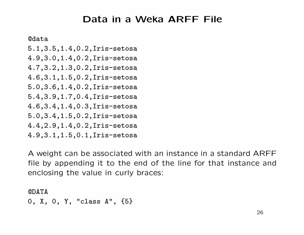
Data in a Weka ARFF File

@data

5.1,3.5,1.4,0.2,Iris-setosa

4.9,3.0,1.4,0.2,Iris-setosa

4.7,3.2,1.3,0.2,Iris-setosa

4.6,3.1,1.5,0.2,Iris-setosa

5.0,3.6,1.4,0.2,Iris-setosa

5.4,3.9,1.7,0.4,Iris-setosa

4.6,3.4,1.4,0.3,Iris-setosa

5.0,3.4,1.5,0.2,Iris-setosa

4.4,2.9,1.4,0.2,Iris-setosa

4.9,3.1,1.5,0.1,Iris-setosa

A weight can be associated with an instance in a standard ARFF

file by appending it to the end of the line for that instance and

enclosing the value in curly braces:

@DATA

0, X, 0, Y, "class A", {5}

26

Data for Weka

Data can also be fed to Weka as CSV files.

Supplying the metadata, however, can be very tedious.

The data can be specified as training or test by keywords, or

else Weka can be told to choose a certain percentage from a full

dataset consisting of both training and test.

27

Using Weka

Weka is run through the Java virtual machine (JVM), which

translates the bytecode.

There is a Microsoft .BAT file that can be invoked through Win-

dows.

Weka can be obtained from

http://www.cs.waikato.ac.nz/~ml/weka/

The best documentation is the paperbound book Data Mining:

Practical Machine Learning Tools and Techniques, third edition,

2011 by Ian H. Witten, Eibe Frank, and Mark A. Hall.

The book also has a lot of general info about statistical learning.

I encourage you to experiment with Weka.

28

The RWeka Package

The R package RWeka provides an R interface to several Weka

meta learners, including AdaBoost, Bagging, LogitBoost, Multi-

BoostAB, Stacking, and CostSensitiveClassifier.

Each of the classification methods has several parameters, which

are passed to the classifier in Weka control.

The control parameter of course are different for each classifier,

and can be determined by use of the function WOW.

The basic function for AdaBoost is AdaBoostM1.

29

AdaBoost in R

> library(RWeka)

> WOW(AdaBoostM1)

P Percentage of weight mass to base training on.

(default 100, reduce to around 90 speed up)

Q Logical variable; use resampling for boosting?

S Random number seed. (default 1)

I Number of iterations. (default 10)

D Logical variable; classifier is run in debug mode

and outputs the results and possibly

additional info to the stdout

W Full name of base classifier. (default:

weka.classifiers.trees.DecisionStump)

30

The “Iris” Dataset

One of the most widely-used datasets for classification is the

“iris” dataset.

The data were collected by a botanist, Edgar Anderson, from

iris plants growing on the Gaspe Peninsula to study geographic

variation in the plants.

The dataset was made famous by R. A. Fisher in 1936.

It consists of 4 measurements and a class indicator. There are

50 instances of each of 3 classes.

It is available at UCI, and is also a built-in dataset in R.

31

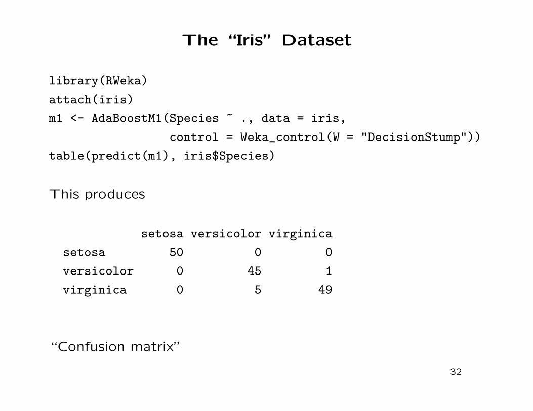
The “Iris” Dataset

library(RWeka)

attach(iris)

m1 <- AdaBoostM1(Species ~ ., data = iris,

control = Weka_control(W = "DecisionStump"))

table(predict(m1), iris$Species)

This produces

setosa versicolor virginica

setosa 50 0 0

versicolor 0 45 1

virginica 0 5 49

“Confusion matrix”

32