testing and interpreting interaction effects in multilevel models · 2017-09-19 · presentation...

Testing and Interpreting Interaction Effects in

Multilevel Models

Joseph J. Stevens

University of Oregon

and

Ann C. Schulte

Arizona State University

Presented at the annual AERA conference, Washington, DC, April, 2016

© Stevens, 2016

1http://www.ncaase.com/

http://www.ncaase.com/



Contact Information:

Joseph Stevens, Ph.D.

College of Education

5267 University of Oregon

Eugene, OR 97403

(541) 346-2445

[email protected]

Presentation available on NCAASE web site: http://www.ncaase.com/

This research was funded in part by a Cooperative Service Agreement from the Institute of

Education Sciences (IES) establishing the National Center on Assessment and Accountability

for Special Education – NCAASE (PR/Award Number R324C110004); the findings and

conclusions expressed do not necessarily represent the views or opinions of the U.S.

Department of Education.


mailto:[email protected]





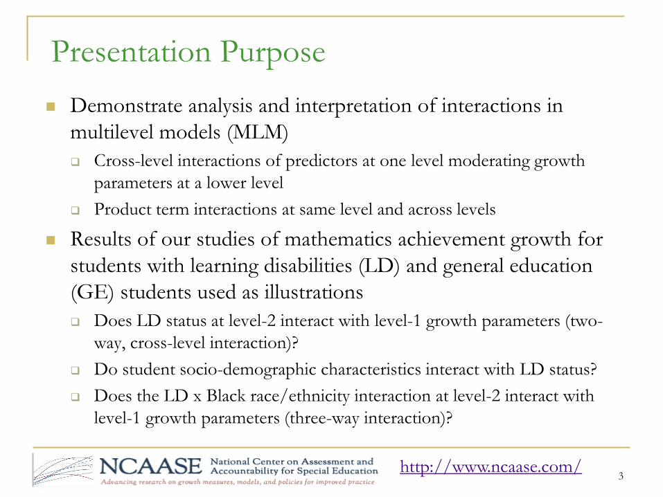
Presentation Purpose

Demonstrate analysis and interpretation of interactions in

multilevel models (MLM)

Cross-level interactions of predictors at one level moderating growth

parameters at a lower level

Product term interactions at same level and across levels

Results of our studies of mathematics achievement growth for

students with learning disabilities (LD) and general education

(GE) students used as illustrations

Does LD status at level-2 interact with level-1 growth parameters (two-

way, cross-level interaction)?

Do student socio-demographic characteristics interact with LD status?

Does the LD x Black race/ethnicity interaction at level-2 interact with

level-1 growth parameters (three-way interaction)?





Cross-level Interactions in Multilevel Models

While many MLM studies incorporate cross-level interactions, it

is much less common for analysts to conduct complete post-hoc

testing when interactions are significant

Level-1 Model: Yti = π0i + π1i*(Timeti) + π2i*(Time2ti) + eti (1)

Level-2 Model: π0i = β00 + β01*(Predictori) + r0i (2)

π1i = β10 + β11*(Predictori) + r1i (3)

π2i = β20 + β21*(Predictori) + r2i (4)

Mixed Model: Yti = β00 + β01*Predictori + β10*Timeti + β11*Predictori*Timeti + β20*Time2ti

+ β21*Predictori*Time2ti + r0i + r1i*Timeti + r2i*Time2

ti + eti (5)





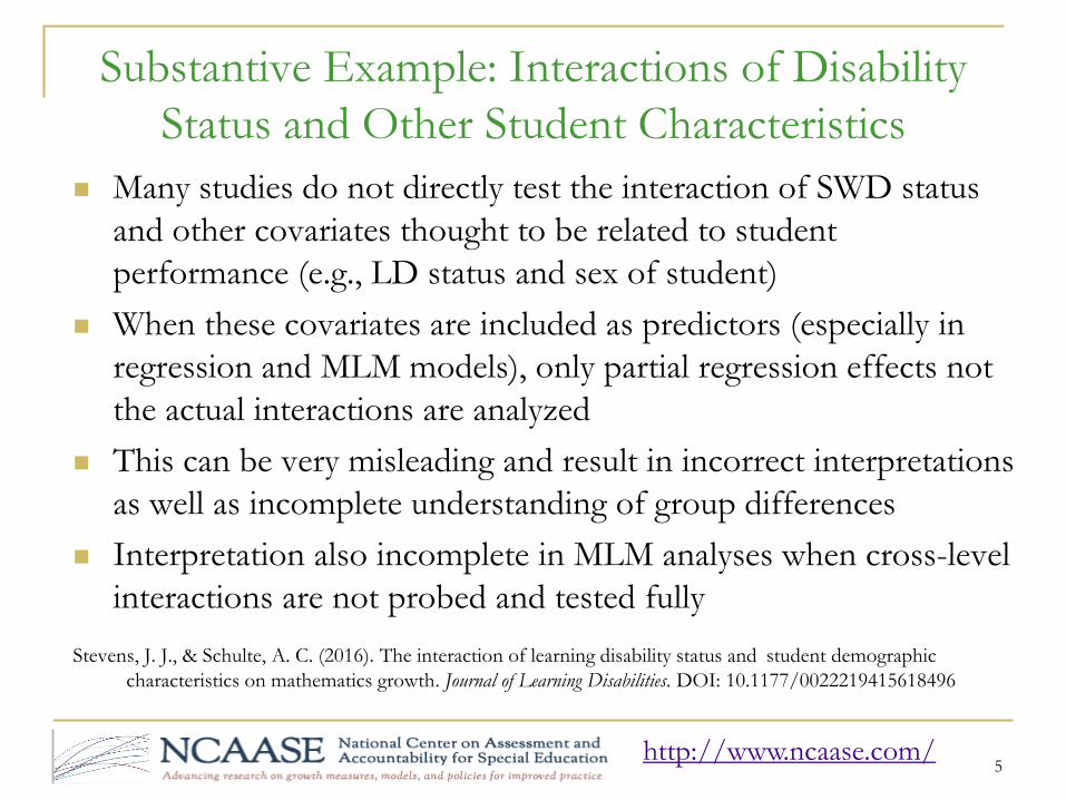
Substantive Example: Interactions of Disability

Status and Other Student Characteristics

Many studies do not directly test the interaction of SWD status

and other covariates thought to be related to student

performance (e.g., LD status and sex of student)

When these covariates are included as predictors (especially in

regression and MLM models), only partial regression effects not

the actual interactions are analyzed

This can be very misleading and result in incorrect interpretations

as well as incomplete understanding of group differences

Interpretation also incomplete in MLM analyses when cross-level

interactions are not probed and tested fully

Stevens, J. J., & Schulte, A. C. (2016). The interaction of learning disability status and student demographic

characteristics on mathematics growth. Journal of Learning Disabilities. DOI: 10.1177/0022219415618496





Examples of Interaction Testing

Student scores on the mathematics subtest of the Arizona

Instrument to Measure Standards (AIMS) used to examine cross-

level interaction of level-2 LD status with level-1 growth

parameters (Grades 3 to 5)

Student scores on the mathematics subtest of the North Carolina

state test used to demonstrate three-way interaction of level-2

LD x Black race/ethnicity with level-1 growth parameters Grades

3 to 7)

Details on sample, methods and procedures available in full

papers





Cross-level Interaction with Level-1 Growth

Parameters

When a level-2 predictor (e.g., LD status) is used to

predict growth at level-1, a two-way, cross-level

interaction is formed

If the cross-level interaction is statistically significant,

post-hoc tests needed to determine specific differences

(e.g., between GE vs. LD groups? From one grade to

another?)

Equivalent to “simple effects” and “simple slopes” post

hoc tests in ANOVA





Two-level Linear MLM Growth Model: AIMS Data

Grades 3 to 5

8

Fixed Effect Coefficient SE t-ratio df p

Intercept, β00 464.148472 0.186455 2489.331 75498 <0.001

LD, β01 -58.878605 0.681264 -86.426 75498 <0.001

LEP, β02 -48.001811 0.382293 -125.563 75498 <0.001

LD X LEP, β03 30.379128 1.128151 26.928 75498 <0.001

Slope, β10 29.396669 0.075204 390.893 75498 <0.001

LD, β11 -3.574548 0.290520 -12.304 75498 <0.001

LEP, β12 0.581080 0.180825 3.214 75498 0.001

LD X LEP, β13 -0.474001 0.515804 -0.919 75498 0.358

Grade

Group 3 4 5

GE 456.66 486.14 515.63

(39.92) (42.79) (45.72)

LD 400.10 425.95 451.81

(28.65) (31.03) (33.44)

_______________________________________________________________

LD x Slope Cross-level Interaction

EB Means for the LD x Slope Cross-level Interaction

9

Figure 1. Cross-level interaction of disability status and grade for the

Arizona sample.

Simple effects of slope for each separate group, horizontal”

analysis within each group

Simple effects differences between the GE vs. LD trajectories,

“vertical” analysis between groups at each time point

Output provides test of simple slope for GE

students, but need to test trajectory for LD students

Simple effect of LD intercept or slope:

Where general formula for SE at moderator value

M is:

SEβ00LD= [SE2(β00) + (2M)cov(β00 , β11) + M2SE2(β11)]

½

10

Simple effects of slope for each separate group

t = βLD / SEβLD


Note. SE formula above for either continuous or dichotomous predictors; simplifies for

dichotomous predictors.




With our dichotomous moderator, when M = 1,

intercept SE:

SEβ0,LD= [SE2(β00) + 2cov(β00 , β01) + SE2(β01)]

½

Slope SE:

SEβ1,LD= [SE2(β10) + 2cov(β10 , β11) + SE2(β11)]

½

11

Simple effect of intercept or slope for each

separate group

Note. When M = 0, formulas simplify to SEβ0,GE= [SE2(β01)]

½ or SEβ1,LD = [SE2(β01)] ½ .





Alpha Adjustment

Repeated testing in post-hoc analysis can result in the inflation

of Type I error (i.e., alpha slippage)

We used Bonferroni's adjustment for post-hoc tests

The nominal alpha level (.05) was divided by the number of

tests within a family of comparisons (see Pedhazur, 1997, p.

435) to create a decision rule that took the number of

comparisons tested into account





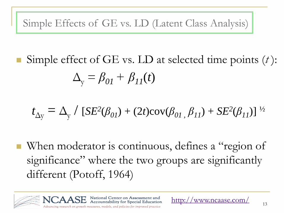
Simple effect of GE vs. LD at selected time points (t ):

Δy = β01 + β11(t)

tΔy = Δy / [SE2(β01) + (2t)cov(β01 , β11) + SE2(β11)] ½

When moderator is continuous, defines a “region of

significance” where the two groups are significantly

different (Potoff, 1964)


Simple Effects of GE vs. LD (Latent Class Analysis)




Example of MLM Three-way Interaction

We were also interested in the product term interaction of

student characteristics at level-2 (e.g., LD x Black race/ethnicity)

and how those groups interacted with growth at level-1

To accomplish this we computed the product of the LD and

Black dummy codes and then used LD, Black and LD x Black as

predictors in a two-level MLM of NC math achievement growth

The predictors were used to model all random growth

parameters (intercept, linear change, curvilinear change) over

five grades





15

Fixed Effect Coefficient SE t df p

Intercept, β00 253.857622 0.040764 6227.510 79544 <0.001

LD, β04 -4.659241 0.110734 -42.076 79544 <0.001

BLACK, β06 -4.401213 0.055501 -79.299 79544 <0.001

LDxBLACK, β09 0.425137 0.194290 2.188 79544 0.029

Linear Slope, β10 7.015400 0.024868 282.103 79544 <0.001

LD, β14 -0.706862 0.071533 -9.882 79544 <0.001

BLACK, β16 0.221137 0.035939 6.153 79544 <0.001

LDxBLACK, β19 -0.405060 0.138214 -2.931 79544 0.003

Curvilinear, β20 -0.526089 0.006246 -84.226 79544 <0.001

LD, β24 -0.008205 0.017716 -0.463 79544 0.643

BLACK, β26 -0.111824 0.008944 -12.502 79544 <0.001

LDxBLACK, β29 0.105315 0.034352 3.066 79544 0.002

Note. Table presented for illustrative purposes. Complete results available in Stevens & Schulte (2016).

MLM Curvilinear Growth Model with LD x Black

Interaction Effect

Conducting Statistical Tests

Process is parallel to AIMS analysis above:

Bonferroni-adjusted simple slope effects; each of the

four interaction groups’ growth trajectories (see Figure

below) calculated by rotating coding of the dichotomous

predictors as described above

Simple effect group differences, also a direct extension of

presentation above (equivalent to a LCA with 3-way

interactions)

We also calculated pairwise comparisons of the four

interaction groups at each point in time (Grade) to allow

specific tests of group differences at each grade





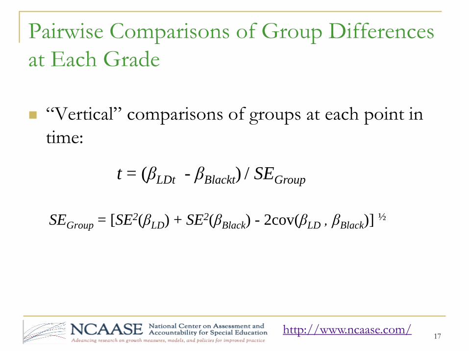
Pairwise Comparisons of Group Differences

at Each Grade

“Vertical” comparisons of groups at each point in

time:

SEGroup = [SE2(βLD) + SE2(βBlack) - 2cov(βLD , βBlack)] ½

17

t = (βLDt - βBlackt) / SEGroup





Level-2 Interaction Means

In the MLM regression equation (LD, Black, and

LD x Black, respectively), a 2 x 2 matrix of the

interaction group means at each grade is:

There are six possible pairwise comparisons among

these four interaction means (k[k-1]/2 = 4[3]/2 = 6)


LD Status

GE, 0 LD, 1

Race/

ethnicity

White, 0 β0 β0 + βLD

Black, 1 β0 + βBL β0 + βLD + βBL + βLDxBL




19

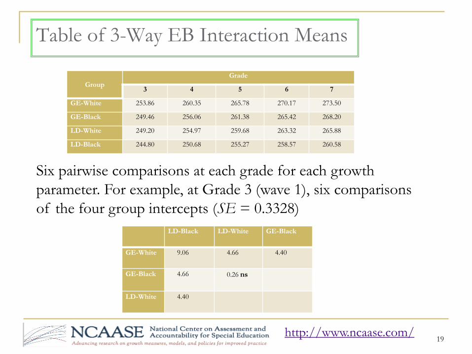
Group

Grade

3 4 5 6 7

GE-White 253.86 260.35 265.78 270.17 273.50

GE-Black 249.46 256.06 261.38 265.42 268.20

LD-White 249.20 254.97 259.68 263.32 265.88

LD-Black 244.80 250.68 255.27 258.57 260.58

Table of 3-Way EB Interaction Means

Six pairwise comparisons at each grade for each growth

parameter. For example, at Grade 3 (wave 1), six comparisons

of the four group intercepts (SE = 0.3328)

LD-Black LD-White GE-Black

GE-White 9.06 4.66 4.40

GE-Black 4.66 0.26 ns

LD-White 4.40





20

Figure 2. Three-way interaction of LD status, black-white race/ethnicity, and

grade for the North Carolina sample.

Brief Bibliography

Aiken, L. S., & West, S. G. (1991). Multiple regression: Testing and interpreting interactions.

Thousand Oaks, CA: Sage.

Bauer, D. J., & Curran, P. J. (2005). Probing interactions in fixed and multilevel regression:

Inferential and graphical techniques. Multivariate Behavioral Research, 40, 373-400.

Curran, P. J., Bauer, D. J, & Willoughby, M. T. (2004). Testing main effects and interactions in

hierarchical linear growth models. Psychological Methods, 9, 220-237.

Hardy, M. A. (1993). Regression with dummy variables. Newbury Park, CA: Sage Publications.

Hayes, A. F. (2013). Introduction to mediation, moderation, and conditional process analysis: A regression-based

approach. New York, NY: Guilford Press.

Jaccard, J., & Turrisi, R. (2003). Interaction effects in multiple regression (2nd ed.). Thousand Oaks, CA:

Sage.

Pedhazur, E. J. (1997). Multiple regression in behavioral research. Orlando, FL: Harcourt Brace.

Potoff, R. (1964). On the Johnson-Neyman technique and some extensions thereof. Psychometrika, 29,

241-256.

Stevens, J. J., & Schulte, A. C. (2016). The interaction of learning disability status and student

demographic characteristics on mathematics growth. Journal of Learning Disabilities.

Advance online publication. doi: 10.1177/0022219415618496





Software Support

PROCESS software:

Hayes, A. F. (2013). Introduction to mediation, moderation, and conditional process analysis: A regression-based

approach. New York, NY: Guilford Press.

http://afhayes.com/spss-sas-and-mplus-macros-and-code.html

Kristopher J. Preacher, interactive calculation tools for probing interactions in multiple linear

regression, latent curve analysis, and hierarchical linear modeling:

http://www.quantpsy.org/interact/


http://afhayes.com/spss-sas-and-mplus-macros-and-code.html

http://www.quantpsy.org/interact/




Appendices

Comparison of partial and interaction effects

HLM screens for obtaining variance-covariance matrix output

variance-covariance matrix output for the HLM two-level AIMS

model with LD status at level-2

23

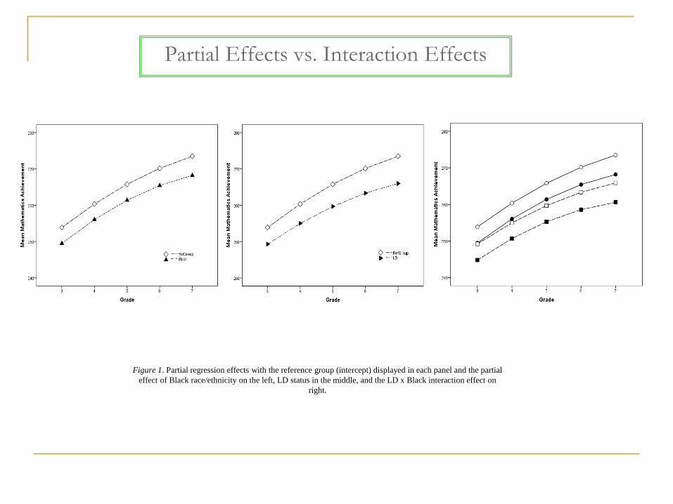
Figure 1. Partial regression effects with the reference group (intercept) displayed in each panel and the partial

effect of Black race/ethnicity on the left, LD status in the middle, and the LD x Black interaction effect on

right.

Partial Effects vs. Interaction Effects

25

HLM Screens Showing Request for Variance-covariance

Matrix Output

27

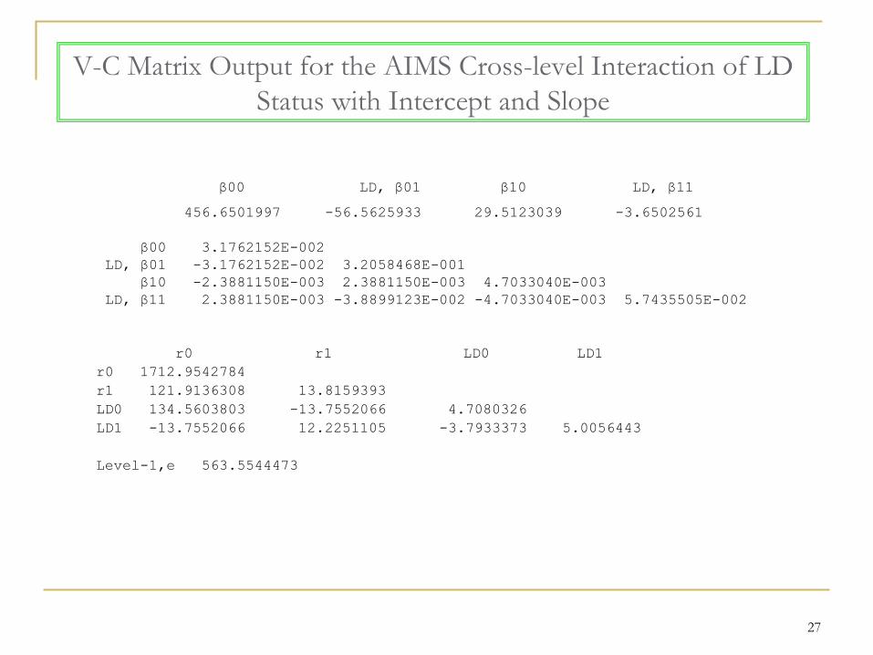
V-C Matrix Output for the AIMS Cross-level Interaction of LD

Status with Intercept and Slope

β00 LD, β01 β10 LD, β11

456.6501997 -56.5625933 29.5123039 -3.6502561

β00 3.1762152E-002

LD, β01 -3.1762152E-002 3.2058468E-001

β10 -2.3881150E-003 2.3881150E-003 4.7033040E-003

LD, β11 2.3881150E-003 -3.8899123E-002 -4.7033040E-003 5.7435505E-002

r0 r1 LD0 LD1

r0 1712.9542784

r1 121.9136308 13.8159393

LD0 134.5603803 -13.7552066 4.7080326

LD1 -13.7552066 12.2251105 -3.7933373 5.0056443

Level-1,e 563.5544473

testing and interpreting interaction effects in multilevel models · 2017-09-19 · presentation...

Documents