testing and analysis of the route 141 newport viaduct ... · testing and analysis of the route 141...

Testing and Analysis of the Route 141

Newport Viaduct: Fatigue Evaluation

By

HARRY W. SHENTON, III

MICHAEL CHAJES

DANIEL KUCZ

JAMES QUIGLEY

JOSE SOTO FUENTES

Center for Innovation Bridge Engineering

University of Delaware

June 2012

Delaware Center for Transportation University of Delaware

355 DuPont Hall

Newark, Delaware 19716

(302) 831-1446

DCT 227

The Delaware Center for Transportation is a university-wide multi-disciplinary research unit reporting to the Chair of the Department of Civil and Environmental Engineering, and is co-sponsored by the University of Delaware and the Delaware Department of Transportation.

DCT Staff

Ardeshir Faghri Jerome Lewis Director Associate Director

Ellen Pletz Earl “Rusty” Lee Matheu Carter Sandra Wolfe Assistant to the Director T2 Program Coordinator T² Engineer Event Coordinator

DCT Policy Council

Natalie Barnhart, Co-Chair Chief Engineer, Delaware Department of Transportation

Babatunde Ogunnaike, Co-Chair Dean, College of Engineering

Delaware General Assembly Member

Chair, Senate Highways & Transportation Committee

Delaware General Assembly Member Chair, House of Representatives Transportation/Land Use & Infrastructure Committee

Ajay Prasad

Professor, Department of Mechanical Engineering

Harry Shenton Chair, Civil and Environmental Engineering

Michael Strange

Director of Planning, Delaware Department of Transportation

Ralph Reeb Planning Division, Delaware Department of Transportation

Stephen Kingsberry

Executive Director, Delaware Transit Corporation

Shannon Marchman Representative of the Director of the Delaware Development Office

James Johnson

Executive Director, Delaware River & Bay Authority

Holly Rybinski Project Manager-Transportation, AECOM

Delaware Center for Transportation University of Delaware

Newark, DE 19716 (302) 831-1446

1

Testing and Analysis of the Route 141 Newport

Viaduct: Fatigue Evaluation

Harry W. Shenton III, Michael J. Chajes, Daniel Kucz, James Quigley, Jose Soto Fuentes

June 2012

i

Table of Contents

1 Introduction .......................................................................................................................................... 1

1.1 Background ................................................................................................................................... 1

1.2 Description of the viaduct ............................................................................................................. 1

1.3 Fatigue cracking ............................................................................................................................ 4

1.4 Objectives of the project ............................................................................................................... 8

1.5 Project timeline ............................................................................................................................. 8

2 Field Testing ........................................................................................................................................ 10

2.1 Introduction ................................................................................................................................ 10

2.2 Controlled Load Tests of Spans 10 and 15 .................................................................................. 10

2.3 In-Service Monitoring of Span 10 ............................................................................................... 27

3 Finite Element Modeling ..................................................................................................................... 36

3.1 Introduction ................................................................................................................................ 36

3.2 Global bridge models .................................................................................................................. 36

3.3 Local Connection Model ............................................................................................................. 47

4 Fatigue Analysis ................................................................................................................................... 54

4.1 Introduction ................................................................................................................................ 54

4.2 Estimating Remaining Life ........................................................................................................... 54

4.3 Global model estimate ................................................................................................................ 55

4.4 Local Model – Field Testing Estimate .......................................................................................... 61

5 Retrofit Options .................................................................................................................................. 69

5.1 Introduction ................................................................................................................................ 69

5.2 Retrofit Options .......................................................................................................................... 69

5.3 Modeling the retrofits ................................................................................................................. 71

5.4 Results of the analysis ................................................................................................................. 73

5.5 Estimated fatigue life of retrofitted designs ............................................................................... 79

6 Summary and Conclusions .................................................................................................................. 82

7 References .......................................................................................................................................... 84

ii

List of Tables

Table 1.1 Newport Viaduct Span Configuration ........................................................................................... 2

Table 2.1 Sensor locations for test – Span 10 ............................................................................................. 14

Table 2.2 Sensor locations for test – Span 15 ............................................................................................. 14

Table 2.3 Truck passes Spans 10 and 15 ..................................................................................................... 16

Table 2.4 Maximum and minimum stresses (ksi) for all strain transducers and test runs, Span 10

(negative denotes compression) .............................................................................................. 18

Table 2.5 Stress range (ksi) for all strain transducers and test runs, Span 10 ............................................ 19

Table 2.6 Maximum and minimum stresses (ksi) for all strain transducers and test runs, Span 15

(negative denotes compression) .............................................................................................. 20

Table 2.7 Stress range (ksi) for all strain transducers and test runs, Span 15 ............................................ 21

Table 2.8 Rainflow histogram data for BDI strain transducers ................................................................... 31

Table 2.9 Rainflow histogram data for foil strain gages ............................................................................. 32

Table 3.1 Comparison of maximum bending stress from field test and S10 model for Pass 1, Pass 3, and

Pass 5 (cross frame data shown shaded) .................................................................................. 45

Table 3.2 Comparison of maximum bending stress from field test and S15 model for Pass 1, Pass 3, and

Pass 5 (cross frame data shown shaded) .................................................................................. 45

Table 3.3 Summary of loading and boundary condition cases ................................................................... 50

Table 3.4 Boundary condition study results (all stresses in ksi) ................................................................. 53

Table 4.1 Stress range from global S10 model at all eight connections ..................................................... 60

Table 4.2 Estimated fatigue life of the eight connections .......................................................................... 60

Table 4.3 Stress at superimposed foil gage location and corresponding weld toe maximum stress, for

varying boundary conditions .................................................................................................... 63

Table 4.4 Effective Stress at weld toe for different cut-off (minimum) stresses ........................................ 64

Table 4.5 SLADTT estimates with 4% exponential growth rate. ................................................................ 65

Table 4.6 Fatigue life results ....................................................................................................................... 67

Table 4.7 Fatigue life results ....................................................................................................................... 68

Table 5.1 Original Model Stresses for Refined Mesh .................................................................................. 74

Table 5.2 Expected Fatigue Life for Original Model .................................................................................... 74

Table 5.3 Stress Results for Positive Attachment with WT’s ...................................................................... 75

Table 5.4 Percent Reduction in Stress Range for WT Positive Attachment ................................................ 76

Table 5.5 Stress Results for Positive Attachment with WT’s at Bottom Flange and Plates at Top Flange . 77

Table 5.6 Percent Reduction in Stress Range for WT’s at Bottom Flange and Plates at Top Flange .......... 77

Table 5.7 Slot Retrofit Stresses and Percent Reduction in Stress Range .................................................... 78

Table 5.8 Stress Results from Removal of Diagonal Element Retrofit ........................................................ 78

Table 5.9 Summary of Stress Range Reductions from retrofit designs ...................................................... 79

Table 5.10 Expected fatigue life for original model and retrofit ................................................................ 81

iii

List of Figures

Figure 1.1 Arial view of viaduct ..................................................................................................................... 2

Figure 1.2 Typical girder cross-section (girder depth is 4 ft for all spans, bottom flange widths vary)........ 3

Figure 1.3 Type F diaphragm ......................................................................................................................... 5

Figure 1.4 Type E diaphragm ........................................................................................................................ 5

Figure 1.5 Photograph of a Type E diaphragm ............................................................................................. 6

Figure 1.6 Typical crack at weld toe of connection plate (DMJM Harris, 2006) ........................................... 7

Figure 1.7 Typical crack showing propagation into base material of the girder web (DMJM Harris, 2006) 7

Figure 2.1 Global layout of instrumentation locations in Span 10 (southbound) at Sections A, B, and C.. 12

Figure 2.2 Typical cross section sketch of gage locations, Spans 10 and 15 (gages A through F are located

1 ft north of the cross frame). .................................................................................................. 12

Figure 2.3 General view of Strain Transducers after Installation ............................................................... 13

Figure 2.4 Global layout of instrumentation locations in Span 15 (southbound) at Sections A, B, and C.. 14

Figure 2.5 Wheel weights (in lbs) and axle configurations for trucks used in load test ............................. 15

Figure 2.6 Time-history plot of the bottom flange gages for pass 1 at all Sections (A, B, C) ...................... 22

Figure 2.7 Time-history plot of the gages on the west girder, west web and west girder cross frames for

pass 1 ........................................................................................................................................ 23

Figure 2.8 Time-history plot of bottom flange gages, Sections A and C, Span 15, truck pass 1 ................. 24

Figure 2.9 Time-history plot of cross frame gages, Sections A and C, Span 15, truck pass 1 ..................... 25

Figure 2.10 Time-history plot of cross frame gages, Section B, Span 15, truck pass 1 ............................... 26

Figure 2.11 Layout of gage locations for in-service monitoring on Span 10 .............................................. 28

Figure 2.12 Weldable strain gage mounted in web gap ............................................................................. 28

Figure 2.13 Strain transducers mounted to web ........................................................................................ 29

Figure 2.14 Rainflow histogram for foil gage #1, bins 2-5. ......................................................................... 33

Figure 2.15 Rainflow histogram for foil gage #1, bins 6-30. ....................................................................... 33

Figure 2.16 Snapshot event #2 cross frame gages. ..................................................................................... 34

Figure 2.17 Snapshot event #2 mid-web and bottom flange gages. .......................................................... 34

Figure 2.18 Snapshot event #2 web gap foil gages #1 & #2. ...................................................................... 35

Figure 2.19 Snapshot event #2 BDI gages adjacent to connection plate. .................................................. 35

Figure 3.1 General view of the S10 (Span 9-11) finite element model ....................................................... 37

Figure 3.2 View of interior of box girders including interior components ................................................. 37

Figure 3.3 View of type E and type F diaphragm FE mesh in interior of boxes .......................................... 38

Figure 3.4 View of negative moment region FE mesh in interior of boxes................................................. 38

Figure 3.5 FE mesh showing rigid links used to connect top flange, haunch, and parapet to deck nodes.40

Figure 3.6 View of typical modeled girder interior – spans 12 to 16 .......................................................... 41

Figure 3.7 FE computed deformed shape span 9-11 for Pass 1 (truck in right shoulder near mid-span of

span 10) .................................................................................................................................... 44

Figure 3.8 FE computed deformed shape span 9-11 for Pass 3 (truck in right lane near mid-span of span

10) ............................................................................................................................................. 44

Figure 3.9 FE computed deformed shape span 9-11 for Pass 5 (truck in left lane near mid-span of span

10) ............................................................................................................................................. 45

iv

Figure 3.10 Bethlehem Steel fabrication drawings of Type E diaphragms. (Bethlehem Steel, 1974) ........ 48

Figure 3.11 Top connection model. Note higher mesh density in web gap region and bolt holes not

aligned with the cross frame member. .................................................................................... 49

Figure 3.12 Bottom connection model. Note higher mesh density in web gap region and bolt holes

aligned with the cross frame member. .................................................................................... 49

Figure 3.13 Boundary condition cases for the top connection model. ...................................................... 50

Figure 3.14 Bottom connection, bottom edge only fixed analysis results. Maximum principal stress

concentrations are highly localized near web gap region. ....................................................... 51

Figure 3.15 Top connection, top edge only fixed. Maximum principal stress concentrations are highly

localized near web gap region. ................................................................................................. 52

Figure 3.16 Top connection, top edge fixed zoomed in view. Maximum principal stress gradient becomes

extreme near weld toe. ............................................................................................................ 52

Figure 4.1 Equation (4.5): Mean Fatigue Life versus Effective Stress ......................................................... 57

Figure 4.2 Direction of stress taken from global S10 model for fatigue evaluation ................................... 59

Figure 4.3 Typical contour plot of stresses in web and connection plate .................................................. 59

Figure 4.4 Foil gage #1 field location superimposed on localized bottom connection model web gap .... 62

Figure 5.1 Sketch of WT to Bottom Flange Connection .............................................................................. 70

Figure 5.2 Remesh of Original Model on Web and Connection Plate ........................................................ 71

Figure 5.3 Model showing WT positive attachment at bottom flange ....................................................... 72

Figure 5.4 Model showing positive top flange connection ......................................................................... 72

Figure 5.5 Model showing slot between web and connection plate .......................................................... 73

1

1 Introduction

1.1 Background

Distortion induced fatigue cracking is a problem found in certain older steel bridges in the United States.

It is typically attributed to deformations that take place in some direction other than the primary load

direction of the member, and is often related to the connection of secondary members to primary

members. It is something that was not accounted for or anticipated in the original design, but often

requires remedial action once the cracking is discovered.

Bridge number 1-501, also known as the Newport Viaduct, is a 19-span steel trapezoidal box girder

bridge that carries State Route 141 over State Route 4, in Newport, Delaware. It was constructed in

1978. During a 2006 inspection of the inside of the box girders (the first internal inspection ever

conducted on the viaduct), cracks were discovered in the web gap region where the diaphragm

connection plate is welded to the girder web. More than 600 individual cracks or crack locations were

identified; cracks were found in all 19 spans. The cracks were generally hairline in nature with lengths

ranging from 1/8 in. to 4 in., and were present on both sides of the connection plates (north and south)

and girder webs (east and west). Visual inspection indicated that 37 of the cracks had propagated into

the base metal of the girder web. As a result the bridge was classified as structurally deficient and

placed on the Delaware Department of Transportation (DelDOT) list of priority bridges (DelDOT, 2007).

AECOM, a national engineering and consulting firm, was hired to develop a repair and retrofit plan for

the viaduct. The University of Delaware Center for Innovative Bridge Engineering was contracted to

provide support to AECOM and DelDOT in the investigation of the cause of the cracks and development

of the repair plans. This report summarizes the work and the findings of the University of Delaware

Center for Innovative Bridge Engineering.

1.2 Description of the viaduct

A map with the location of the bridge is shown in Figure 1.1. The main structure has 19 spans which

consist of multiple welded steel tub girders with a composite concrete deck. Of the 19 spans, 15 are

continuously supported and 4 are simply supported. The spans are numbered 1 through 19 starting

from the south. In addition to the main structure, there are ramps on the east and west sides of the

bridge linking Route 141 to local roads.

2

Figure 1.1 Arial view of viaduct

Traffic travels in both northbound and southbound directions, each with its own structure. There is an

open joint between the northbound and southbound structures, resulting in the two independent

structures. Each structure carries two 12 ft. wide travel lanes and a 12 ft. wide right side shoulder. A

narrow (2ft.) left shoulder makes up the remainder of the roadway surface. Each span has between 2

and 4 girders and a concrete composite deck. The depth of the girders is uniform at 4 ft. but the bottom

flange widths vary from span to span. Span configurations are listed in Table 1.1.

Table 1.1 Newport Viaduct Span Configuration

Span # Span

Configuration Span Length # Girders and width

1

Four-span continuous

90'-0"

3-box (4' deep, 6'-6" wide bottom flange) 2 110'-0"

3 130'-0"

4 109'-1"

5 Three-span continuous

99'-1" 3-box (4' deep, bottom flange varies from 6'-6" to 8'-

6" wide) 6 100'-0"

7 99'-1"

8 Simple 101'-9" 4-box (4' deep, 4 girders w/ 9'-0" bott flange, 4

girders w/ 5'-0" bott flange)

9 Three-span continuous

97'-1" 2-box (4' deep, bottom flange varies from 9'-6" to 8'-

0" wide) 10 100'-0"

11 99'-1"

12 Five-span

continuous

118'-0"

2-box (4' deep, 8'-0" wide bottom flange) 13 118'-0"

14 118'-0"

3

15 118'-0"

16 118'-0"

17 Simple 83'-10 5/8" (tangent

from pier 16) 2-box (4' deep, 8'-0" ± 1/16" wide bottom flange)





A typical cross section of a girder is shown in Figure 1.2. The steel girders are welded plates forming a

trapezoidal cross section. The girder webs are angled at a 4:1 slope and have a depth of 4 ft., as such,

the distance between the top flanges of the girders vary with the bottom flange width. The thickness of

the web and flanges varies with span and location.

The nominal thickness of the concrete deck is 9 in., but this varies with location. Between girders, a

constant thickness of 9 in. is specified. Otherwise the depth varies between a low of 6 in. on the outside

edge, to a maximum of almost 16 in. over some of the haunches. To achieve composite action with the

deck, shear studs are welded to the top flanges of the box girders. They are specified to be 0.875 in.

diameter shear studs with a 1.375 in. diameter head configured in rows of three. The length of the

shear studs varies depending on the flange location, but they are specified to extend a minimum of 2 in.

beyond the bottom layer of deck re-bar not surpassing the top layer.

Figure 1.2 Typical girder cross-section (girder depth is 4 ft for all spans, bottom flange widths vary)

Internal diaphragms are spaced longitudinally throughout the girders to provide stability and to increase

the torsional stiffness of the structure. Two types of internal diaphragms are used for this purpose,

“Type E” and “Type F”. The Type F diaphragm is a steel 7 in. x 4 in. x 3/8 in. angle bolted to connection

plates just below the top flanges on both sides of the girder. Layout and dimensions of the Type F

4

1

10 ft.

8 ft.

4 ft.

4

diaphragm are shown in Figure 1.3. The connection plates are 3/8” thick and are welded to the girder

web a minimum of 2 ½ in. below the bottom of the top flange to just beyond the depth of the angle.

The Type E diaphragm is a Type F diaphragm with the addition of two 3 in. x 3 in. x 3/8 in. steel angles

oriented diagonally to form an x-type brace, and longer connection plates. The angles are connected at

their ends to the respective plates and angles, but are not connected to each other where they cross.

The connection plates for the Type E diaphragms are also 3/8 in. thick steel plates that are welded to the

webs. The Type E connection plates extend from below the top flange to above the bottom flange.

Details specify that a minimum distance of 2 1/2 in. must be maintained between the top or bottom of

the connection plate and the nearby flange. The cross frame angles are bolted to the bottoms of the

connection plates and to the 7 in. x 4 in. x 3/8 in. horizontal angle with two bolts at each connection.

Layout and dimensions of the Type E diaphragm are shown in Figure 1.4. A photograph of the Type E

diaphragm is shown in Figure 1.5. A typical girder has the Type E and Type F diaphragms alternated,

spaced at approximately 24 ft throughout the span.

Increased stiffness is provided at the negative moment regions of the continuous spans. This comes

from additional steel members added to the interior of the girder. On top of the bottom flange, five 5 x

10.5 structural tees are welded at even intervals between the girder webs. These run longitudinally in

the negative moment region from 3 in. inside of one splice plate to 3 in. inside the next splice plate.

Above and perpendicular to the WT’s, C 20.7 structural channels are welded to each side of the girder

web. The bottom flanges of the channels rest on the top flange of the WT’s and they are welded where

there is contact. These are spaced at approximately 6 ft.-6 in. typically resulting in 4 lateral channels on

either side of each pier.

The steel properties in the trapezoidal boxes vary by location along the length of the spans and by

component. A572 Grade 50 steel (fy = 50ksi) is specified in many of the negative moment regions, and

A36 steel (fy = 36 ksi) is specified in the positive moment regions. The concrete deck superstructure was

specified to have a 28-day compressive strength of 4,500 psi (f’c = 4.5 ksi).

1.3 Fatigue cracking

Construction of the viaduct was completed in 1978. The first ever interior inspection of the girders was

conducted in the fall of 2006. The conclusion of the 2006 Interior Box Inspection Report (DMJM Harris,

2006) was an overall good condition of the structure existed with the exception of cracked welds

between the Type E diaphragm connection plates and the box girder webs. In total, 655 cracks were

found; the cracks were hairline in width with lengths varying from 1/8 in. to 4 in. and occurred only at

Type E diaphragm locations. As a result of the extensive and widespread cracking, recommendations

were made to monitor the current cracked locations with particular attention to cracks that appear to

have propagated into the girder webs.

5

10'

Typ. Gap212"

1'-2"

34"

8'

34"

4'

12"

L 7 x 4 x 3/8 7 x 3/8

Connection

Plate

1'-2"

34"

Figure 1.3 Type F diaphragm

10'

212" Typ.

34"

1'-2"

7 x 3/8

Connection

PlateL 3 x 3 x 3/8

L 7 x 4 x 3/8

12"

4'

34"

8'

34"

1'-2"

Figure 1.4 Type E diaphragm

6

Figure 1.5 Photograph of a Type E diaphragm

Since the 2006 Interior Box Inspection Report, 52 crack locations were identified as requiring retrofit. Of

these, 10 locations were selected as candidates for core sampling in which more extensive metallurgical

examination would be carried out (DMJM Harris, 2006).

Fatigue cracking in the structure is present at the weld between the Type E diaphragm connection plates

and the girder webs. The connection plates are fillet welded to the girder webs along their entire

length, with the weld extending underneath the connection plate end termination. Cracking is present

at both the top and bottom of the connection plate termination and on both sides of the connection

plate (north and south). Typically, the cracks follow the edge of the fillet weld on the underside of the

stiffener and extend vertically along the interface of the connection plate fillet weld. Along the

underside of the connection plate, the fatigue cracks are generally located at the connection plate end

near the weld root. As they propagate, the cracks cross through the weld material to the weld toe

interface. In some cases, the cracks have propagated outward from the interface of the connection

plate fillet weld and extend into the girder web material (Figure 1.6, Figure 1.7).

7

Figure 1.6 Typical crack at weld toe of connection plate (DMJM Harris, 2006)

Figure 1.7 Typical crack showing propagation into base material of the girder web (DMJM Harris, 2006)

Six cracks were removed from the Newport Viaduct as core samples, and were taken to Lehigh

University for examination. The cracks were determined to be a result of fatigue initiation. The cracks

initiated in the weld metal and propagated towards the web through the weld. Evidence of repeated

crack initiation suggests that the crack propagation was due to out-of-plane web distortions. There was

no visual evidence of weld defects, signifying that the crack initiated at normal defects within the weld

toes. As is expected with this type of fatigue stress, the cracks started in the longitudinal direction and

8

either turned to run transverse along the web, or were expected to do so if propagation had continued

(Kaufmann, 2008).

1.4 Objectives of the project

The objectives of the project were to conduct field tests of sections of the viaduct and develop detailed

finite element models that would be used to conduct a fatigue evaluation of the viaduct, and to assist in

developing a repair and retrofit strategy for the viaduct. The specific objectives were:

1. Conduct diagnostic load tests of sections of the viaduct to measure the strains induced by loads

of known weight. The data from the tests would be used to calibrate finite element models of

the viaduct.

2. Conduct in-service monitoring due to the site specific traffic of one or more crack prone details

to estimate the true effective stress range at the detail.

3. Develop global finite element models of two different sections of the bridge; calibrate the

models using the results of the controlled load tests.

4. Develop a detailed 3D finite element model of the connection and analyze it for various load

condition.

5. Use the global and local finite element models to estimate effective stress in the crack location

and conduct a fatigue evaluation and remaining life study of the fatigue prone details.

6. Use the global finite element model to study various retrofit options and provide

recommendations on the effectiveness of each.

1.5 Project timeline

Work on the project began in the fall of 2007 and continued through the spring of 2011. The actual work

by the consultant began sometime after UD commenced working on the project, and AECOM completed

their tasks before the UD work was completed. However, the results of the UD study were used by the

consultant in developing their final retrofit plans.

The results are documented in three separate Master’s thesis’ from the University of Delaware, these

are:

“Analysis of distortion-induced fatigue cracking of a trapezoidal steel box girder bridge including

retrofit investigation,” by James R. Quigley, Spring 2009

“Analysis of distortion-induced fatigue cracking in a steel trapezoidal box girder bridge,” by

Daniel A. Kucz, Spring 2009

“Fatigue life analysis of a steel trapezoidal box girder bridge using measured strains,” by Jose

Soto Fuentes, Spring 2011

All of the details of the work reported herein is included in the above mentioned thesis’.

The remainder of the report is organized as follows:

9

Chapter 2 – describes the field tests that were conducted. This includes the diagnostics tests of

spans 10 and 15, and the in-service monitoring that was conducted on span 10.

Chapter 3 – describes the global finite element models that were developed of spans 10 and 15,

and the local finite element models of the connections.

Chapter 4 – the fatigue evaluation is reported in this chapter.

Chapter 5 – retrofit options are presented and the results of the retrofitted finite element

models are described.

Chapter 6 – conclusions and recommendations

10

2 Field Testing

2.1 Introduction

Two controlled load tests were conducted on the viaduct for the purpose of gathering data to calibrate

the finite element models of the bridge. Span 10 was tested on December 17, 2008, and Span 15 was

tested on December 18, 2008. In-service monitoring was also conducted on Span 10 for the purpose of

measuring the actual effective stress near the connection due to the site specific traffic. The in-service

monitoring commenced on November 17, 2010 and continued around the clock, for 23 days. Presented

below is a summary of these tests and the results.

2.2 Controlled Load Tests of Spans 10 and 15

Test Setup – Span 10

The Bridge Diagnostics Inc. (BDI), Structural Testing System (STS) was used to conduct the controlled

load tests. The system consists of strain transducers, 4-channel data acquisition junction boxes, and a

main power supply/control system. The BDI strain transducers have a gage length of three inches, and

are either clamped to a member using C-clamps, or when that is not possible, bonded to the surface

using a quick setting 2-part adhesive. Once the sensors are mounted they are connected to the junction

boxes, which in turn are daisy-chained with trunk cables back to the main power supply/control system.

The STS is operated from a laptop computer that is connected to the control system.

A total of 23 strain transducers were mounted near three Type E cross frames in span 10. The overall

layout of the test is shown in Figure 2.1. On the interior (east) girder, transducers were placed near the

Type E diaphragms in the positive moment region, numbered XF2 and XF3 from the south (Section A and

Section B, respectively). On the exterior (west) girder, transducers were places near XF2 only (Section

C). The sensors were deployed in this fashion to capture the overall structural behavior longitudinally

and transversely of the viaduct.

Strains due to bending were measured by installing transducers on the bottom flange, mid-height, and

top flange of the girder on both webs (east and west) at each section (A,B,C). To avoid local out-of-plane

effects induced by the Type E diaphragms, the sensors were offset a distance of 1 ft. to the north of the

cross frame. Axial strains in the Type E diaphragm cross frame members were measured by clamping

the transducers directly to one leg of the members (note that the sensors were placed on the

outstanding leg of the angle, i.e., the one that was not bolted to the connection plate). For the gages

installed on the box girder with adhesive, the surface was prepared by grinding through the protective

paint layer to the structural steel. The sensor designations (numbers) and their locations are listed in

Table 2.1. A typical cross section showing the layout of the strain sensors is shown in Figure 2.2. Figure

2.3 shows general views of the transducers after installation.

11

Test Setup Span 15

The span 15 setup was very similar to the span 10 setup. A total of 23 strain gages were mounted near

three Type E cross frame locations in span 15. The overall layout of the test is shown in Figure 2.4. The

sensor numbers and their locations are listed in Table 2.5

12

Figure 2.1 Global layout of instrumentation locations in Span 10 (southbound) at Sections A, B, and C

314"

2'

4"4"

2'

314"

Gage HGage G

Gage F

Gage E

Gage DGage C

Gage B

Gage A

Figure 2.2 Typical cross section sketch of gage locations, Spans 10 and 15 (gages A through F are located

1 ft north of the cross frame).

Bottom CrackBottom Crack

Top Crack Top Crack

A

A

B

B

C

C

Exterior Girder

(West)

Interior Girder

(East)

Pier 10

BDI STS Boxes

10 ft. Typ.

N

Pier 9

Type E Diaph

Type F Diaph XF1 XF2 XF3 XF4

13

Transducers mounted to flanges and web

Figure 2.3 General view of Strain Transducers after Installation

Transducers mounted to cross frames

14

Interior Girder

Exterior Girder

Type E

Traffic Flow

North

12 ft. Typical

Type F

Diaphram BDiaphram A

Diaphram C

Pier 14

Cross Section 1 Cross Section 2

Figure 2.4 Global layout of instrumentation locations in Span 15 (southbound) at Sections A, B, and C Table 2.1 Sensor locations for test – Span 10

Location (Looking South) Sensor

Diaphragm A Diaphragm B Diaphragm C

A: Top Flange Left 302 344 298

B: Left Web 535 314 293

C: Bottom Flange Left 356 355 303

D: Bottom Flange Right 292 295 317

E: Right Web 339 337 346

F: Top Flange Right 299 306 348

G: Cross frame 1 338 - 294

H: Cross frame 2 1477 1475 318

Table 2.2 Sensor locations for test – Span 15

Location (Looking South) Sensor

Diaphragm A Diaphragm B Diaphragm C

A: Top Flange Left 295 302 344

B: Left Web 317 348 298

C: Bottom Flange Left 293 337 356

D: Bottom Flange Right 314 292 355

E: Right Web 338 306 339

F: Top Flange Right 299 535 303

G: Cross frame 1 - 1475 346

15

H: Cross frame 2 318 1477 294

Test Vehicles and Passes

DelDOT provided two 3-axle, 10-wheel fully loaded dump trucks for the live loads for the tests. The truck

loads were field measured using InterComp PT300 portable wheel scales which have an accuracy of +/-

10 lbs. The gross vehicle weights were 53.49 kips and 52.97 kips for trucks #314 and #2886,

respectively. For Truck #314, the centerline distance from the front axle to the middle axle was 15 ft. 5

in. For Truck #2886, this distance was 13 ft. 11 in. For both trucks, the distance from the middle axle to

the rear axle was 4 ft. 6 in. A detailed drawing of the truck wheel weights and axle spacings is shown in

Figure 2.5.

Figure 2.5 Wheel weights (in lbs) and axle configurations for trucks used in load test

Truck #314 Truck #2886

87

40

915

0

945

09480

8140

85

30

90

30

8380

87

70

886

0

87

70

8560

86 in

74 in

85 in

73 in

185 in

54 in 54 in

167 in

16

During the tests the local traffic on the bridge was stopped. In all load cases, the trucks traveled in the

southbound direction. For the Span 10 test the trucks were staged just north of Span 11 until

measurements were started. After balancing the strain transducers, the trucks proceeded at a crawl

speed of approximately 5-10 mph across the structure. Strain readings were taken at a rate of 20

samples-per-second. After the truck exited Span 9 (the last span of the three span continuous section),

the recording was stopped. A similar procedure was used for Span 15, with the vehicles staging just

north of Span 16 and recording continued until the vehicle was off of the continuous span, i.e., off of

Span 12.

A total of eight truck passes were made, varying the transverse positions of the trucks on the roadway.

For each lane that could accommodate a truck (Right Shoulder, Right Lane, and Left Lane), two passes

were made, one for each truck (#314, #2886) for a total of six single truck passes. The last two load

passes consisted of side-by-side trucks passes with the vehicles in the Right Shoulder/Right Lane and the

Right Lane/Left Lane, respectively. The truck runs are listed in Table 2.3

Table 2.3 Truck passes Spans 10 and 15

Pass Truck ID Truck Location

1 314 Right shoulder

2 2886 Right shoulder

3 314 Right lane

4 2886 Right lane

5 314 Left lane

6 2886 Left lane

7 314 & 2886 Right shoulder/right lane respectively

8 314 & 2886 Right lane/left lane respectively

Results Span 10

Presented in Table 2.4 are the maximum and minimum recorded stresses for each sensor location, for

each truck pass. Table 2.5 lists the corresponding stress ranges (maximum stress minus the minimum

stress) for each sensor location. These results are based on the measured strains, using a Modulus of

Elasticity for steel of 29,000 ksi. Presented in Figure 2.5 are typical time history plots of the recorded

stress in the bottom flange gages for truck pass 1. Presented in Figure 2.6 are typical plots of the

recorded stress in the west web of the exterior girder and cross frames for truck pass 1. These plots

illustrate the characteristic behavior of the three-span continuous bridge for the sensor readings on the

center span, with the girder experiencing first negative bending, then positive bending, and finally

negative bending again. The maximum positive bending occurs at gage 317, which is consistent with the

truck being in the right shoulder of the bridge.

The absolute maximum stress recorded during the test was 1.87 ksi at gage 295 (bottom flange, west

side, section B) in truck pass 8. The absolute minimum stress recorded was -0.61 ksi in gage 294 (cross

frame and truck pass 8). The absolute maximum stress range was 2.42 ksi in gage 295 for truck pass 8.

For the cross frames, the maximum stress range recorded was 0.70 ksi in gage 294. Other results of the

17

test showed that the neutral axis of the girder was located in the concrete deck, just above the steel

girder top flange. Many more results of the test conducted on span 10 can be found in Kucz (2009).

Results Span 15

Presented in Table 2.6 are the maximum and minimum recorded stresses for each sensor location, for

each truck pass. Table 2.7 lists the corresponding stress ranges for each sensor location. These results

again are based on the measured strains, using a Modulus of Elasticity for steel of 29,000 ksi.

The absolute maximum stress recorded during the test was 2.68 ksi at gage 355 (bottom flange, west

side, section C) in truck pass 7. The absolute minimum stress recorded was -0.75 ksi at gage 337 (bottom

flange, east side, section B) in truck pass 8. The absolute maximum stress range was 3.43 ksi in gage 355

for truck pass 7. For the cross frames, the maximum stress range recorded was 0.68 ksi in gage 318 and

truck pass 7.

Presented in Figure 2.7 is a plot of the bottom flange gages in Sections A and C for truck pass 1. Similar

to the Span 10 results, this plot shows a similar behavior for the 5-span continuous section. Since span

15 is the second span of the 5, the sensor first reads compression when the vehicle is in span 16, it then

goes into tension when the load is within span 15, and then back into compression when it has moved

onto span 14. A small tensile stress is evident when it is in span 13 and the instrumented section feels

very little of the load when it is in the last span, span 12. The transverse distribution of stress is also

apparent from the plot. For pass 1 the vehicle is in the right shoulder, thus the west girder carries a

majority of the load, thus the stresses are highest in that girder. Figures 2.8 and 2.9 show the stresses in

the cross frames at all sections for truck pass 1. One member experiences compression while the other

experiences tension. Thus, in addition to the overall bending that it experiences, the box girder is being

skewed from its undeformed configuration, which causes the tension in one brace and compression in

the other. The behavior was typical for both spans and all sections. Many more results of the test

conducted on span 15 can be found in Quigley (2009).

18

Table 2.4 Maximum and minimum stresses (ksi) for all strain transducers and test runs, Span 10 (negative denotes compression)

Gage

located on: Gage ID Run 1 Run 2 Run 3 Run 4 Run 5 Run 6 Run 7 Run 8

Max Min Max Min Max Min Max Min Max Min Max Min Max Min Max Min

Sec

tion A

top flange 299 0.03 -0.07 0.02 -0.06 0.04 -0.05 0.02 -0.05 0.14 -0.08 0.17 -0.10 0.07 -0.11 0.08 -0.12

mid-web 339 0.04 -0.01 0.05 -0.04 0.14 -0.07 0.14 -0.05 0.33 -0.05 0.35 -0.05 0.33 -0.08 0.41 -0.09

bottom flange 292 0.37 -0.23 0.38 -0.22 0.84 -0.37 0.80 -0.23 1.03 -0.27 1.03 -0.28 1.41 -0.47 1.70 -0.48

cross frame B1477 0.07 -0.13 0.07 -0.14 0.07 -0.22 0.04 -0.19 0.11 -0.10 0.08 -0.03 0.07 -0.31 0.04 -0.14

top flange 302 0.02 -0.03 0.01 -0.02 0.02 -0.01 0.02 -0.02 0.13 -0.02 0.11 0.00 0.02 -0.03 0.13 -0.02

mid-web 535 0.04 -0.08 0.04 -0.08 0.04 -0.14 0.03 -0.12 0.08 -0.07 0.08 -0.07 0.06 -0.18 0.03 -0.16

bottom flange 356 0.18 -0.21 0.21 -0.21 0.55 -0.45 0.40 -0.26 1.22 -0.36 1.16 -0.36 0.74 -0.49 1.51 -0.56

cross frame 338 0.11 -0.04 0.10 -0.05 0.17 -0.03 0.17 -0.03 0.03 -0.08 0.03 -0.06 0.27 -0.04 0.11 -0.02

Sec

tion B

top flange 306 0.04 -0.04 0.03 -0.05 0.03 -0.07 0.03 -0.05 0.12 -0.06 0.17 -0.08 0.08 -0.12 0.07 -0.10

mid-web 337 0.04 -0.06 0.03 -0.07 0.05 -0.22 0.03 -0.21 0.09 -0.29 0.10 -0.31 0.07 -0.38 0.09 -0.46

bottom flange 295 0.40 -0.21 0.44 -0.23 1.01 -0.39 0.85 -0.24 1.16 -0.34 1.16 -0.32 1.55 -0.48 1.87 -0.55

cross frame B1475 0.05 -0.09 0.04 -0.10 0.03 -0.14 0.03 -0.12 0.07 -0.04 0.04 -0.03 0.05 -0.19 0.01 -0.08

mid-web 344 0.02 -0.03 0.02 -0.04 0.03 0.00 0.03 -0.01 0.12 -0.02 0.09 -0.02 0.02 -0.03 0.13 0.00

top flange 314 0.03 -0.08 0.03 -0.09 0.08 -0.11 0.03 -0.08 0.42 -0.13 0.36 -0.11 0.06 -0.10 0.36 -0.15

bottom flange 355 0.15 -0.18 0.18 -0.19 0.53 -0.40 0.35 -0.24 1.37 -0.39 1.22 -0.39 0.65 -0.43 1.55 -0.57

Sec

tio

n C

cross frame 294 0.37 -0.08 0.38 -0.09 0.04 -0.38 0.03 -0.36 0.10 -0.31 0.09 -0.30 0.11 -0.16 0.10 -0.61

mid-web 293 0.58 -0.12 0.58 -0.12 0.92 -0.24 0.91 -0.14 0.39 -0.16 0.38 -0.16 1.19 -0.25 1.20 -0.28

top flange 298 0.16 -0.03 0.16 -0.03 0.23 -0.02 0.24 -0.02 0.02 -0.03 0.00 -0.05 0.18 -0.02 0.20 -0.03

bottom flange 303 0.86 -0.33 0.93 -0.31 1.22 -0.45 1.20 -0.30 0.45 -0.27 0.47 -0.25 1.76 -0.58 1.59 -0.50

top flange 348 0.20 -0.04 0.21 -0.05 0.02 -0.04 0.04 -0.04 0.02 -0.04 0.02 -0.04 0.16 -0.10 0.04 -0.08

mid-web 346 0.66 -0.11 0.69 -0.11 0.43 -0.17 0.39 -0.12 0.15 -0.10 0.13 -0.10 0.91 -0.19 0.52 -0.20

bottom flange 317 1.23 -0.33 1.32 -0.31 0.57 -0.38 0.49 -0.27 0.14 -0.19 0.12 -0.17 1.53 -0.51 0.61 -0.38

cross frame 318 0.05 -0.11 0.06 -0.09 0.11 -0.03 0.13 -0.02 0.09 -0.03 0.07 -0.03 0.04 -0.05 0.19 -0.03

19

Table 2.5 Stress range (ksi) for all strain transducers and test runs, Span 10

Gage


Sec

tion A

top flange 299 0.10 0.08 0.08 0.07 0.22 0.27 0.19 0.20

mid-web 339 0.05 0.09 0.21 0.19 0.39 0.40 0.40 0.49

bottom flange 292 0.60 0.60 1.21 1.04 1.31 1.31 1.88 2.18

cross frame B1477 0.20 0.21 0.29 0.24 0.21 0.11 0.38 0.18

top flange 302 0.05 0.03 0.03 0.03 0.15 0.11 0.05 0.15

mid-web 535 0.12 0.11 0.18 0.15 0.15 0.15 0.25 0.20

bottom flange 356 0.40 0.42 1.01 0.65 1.58 1.52 1.23 2.08

cross frame 338 0.15 0.15 0.20 0.20 0.11 0.09 0.31 0.13

Sec

tion B

top flange 306 0.08 0.08 0.10 0.08 0.18 0.25 0.20 0.17

mid-web 337 0.10 0.10 0.28 0.24 0.38 0.41 0.45 0.55

bottom flange 295 0.62 0.67 1.40 1.09 1.49 1.48 2.03 2.42

cross frame B1475 0.14 0.14 0.17 0.15 0.11 0.07 0.24 0.10

mid-web 344 0.05 0.05 0.03 0.03 0.14 0.10 0.05 0.14

top flange 314 0.11 0.13 0.19 0.11 0.55 0.47 0.16 0.50

bottom flange 355 0.33 0.37 0.93 0.59 1.75 1.62 1.08 2.13

Sec

tio

n C

cross frame 294 0.45 0.47 0.42 0.38 0.42 0.38 0.27 0.70

mid-web 293 0.70 0.70 1.16 1.05 0.55 0.55 1.44 1.48

top flange 298 0.19 0.19 0.25 0.25 0.05 0.05 0.20 0.24

bottom flange 303 1.19 1.24 1.66 1.49 0.72 0.72 2.33 2.08

top flange 348 0.24 0.26 0.06 0.08 0.06 0.06 0.26 0.12

mid-web 346 0.77 0.80 0.61 0.52 0.25 0.23 1.10 0.71

bottom flange 317 1.56 1.63 0.95 0.76 0.33 0.30 2.04 0.99

cross frame 318 0.15 0.15 0.14 0.15 0.12 0.10 0.09 0.22

20

Table 2.6 Maximum and minimum stresses (ksi) for all strain transducers and test runs, Span 15 (negative denotes compression)

Gage

located on: Gage

ID

Run 1 Run 2 Run 3 Run 4 Run 5 Run 6 Run 7 Run 8

Max Min Max Min Max Min Max Min Max Min Max Min Max Min Max Min

Sec

tion A

A: Top Flange Left 295 0.02 -0.02 0.03 -0.02 0.02 -0.01 0.04 -0.01 0.17 -0.01 0.14 -0.01 0.03 -0.02 0.16 -0.01

B: Left Web 317 0.09 -0.12 0.06 -0.11 0.17 -0.16 0.14 -0.11 0.89 -0.23 0.81 -0.20 0.23 -0.18 0.87 -0.29

C: Bottom Flange Left 293 0.33 -0.30 0.30 -0.20 0.65 -0.38 0.63 -0.33 1.70 -0.44 1.68 -0.41 0.99 -0.52 2.16 -0.68

D: Bottom Flange Right 314 0.53 -0.28 0.52 -0.23 1.16 -0.29 1.00 -0.27 1.00 -0.25 1.14 -0.25 1.68 -0.45 2.03 -0.45

E: Right Web 338 0.08 -0.10 0.08 -0.06 0.30 -0.14 0.26 -0.10 0.62 -0.18 0.64 -0.17 0.49 -0.17 0.88 -0.28

F: Top Flange Right 299 0.05 -0.09 0.05 -0.09 0.05 -0.10 0.05 -0.10 0.05 -0.10 0.10 -0.12 0.07 -0.19 0.07 -0.20

H: Cross frame 2 318 0.19 -0.47 0.70 -0.23 0.04 -0.57 0.09 -0.70 0.81 -0.21 0.40 -0.49 0.09 -1.52 0.23 -0.16

Sec

tion B

A: Top Flange Left 302 0.02 -0.29 0.02 -0.27 0.02 -0.39 0.02 -0.34 0.11 -0.08 0.08 -0.06 0.03 -0.56 0.10 -0.19

B: Left Web 348 0.07 -0.03 0.03 -0.03 0.16 -0.03 0.10 -0.03 0.93 -0.02 0.81 -0.02 0.14 -0.05 0.80 -0.03



E: Right Web 306 0.08 -0.28 0.06 -0.32 0.25 -0.33 0.21 -0.30 0.42 -0.30 0.44 -0.33 0.43 -0.61 0.62 -0.54

F: Top Flange Right 535 0.04 -0.09 0.05 -0.09 0.05 -0.11 0.05 -0.11 0.05 -0.13 0.12 -0.13 0.08 -0.18 0.06 -0.22

G: Cross frame 1 1475 0.25 -0.06 0.25 -0.06 0.36 -0.03 0.33 -0.03 0.09 -0.23 0.07 -0.16 0.55 -0.08 0.12 -0.06

H: Cross frame 2 1477 0.08 -0.21 0.08 -0.20 0.03 -0.30 0.03 -0.27 0.18 -0.07 0.14 -0.06 0.08 -0.43 0.04 -0.17

Sec

tio

n C

A: Top Flange Left 344 0.12 -0.02 0.12 -0.02 0.19 -0.02 0.22 -0.02 0.02 -0.05 0.02 -0.05 0.19 -0.02 0.19 -0.04

B: Left Web 298 0.45 -0.13 0.42 -0.15 1.05 -0.18 0.98 -0.16 0.46 -0.19 0.49 -0.19 1.26 -0.24 1.37 -0.28



E: Right Web 339 0.93 -0.19 0.91 -0.16 0.48 -0.17 0.50 -0.15 0.18 -0.12 0.22 -0.13 1.10 -0.28 0.63 -0.28

F: Top Flange Right 303 0.25 -0.02 0.25 0.00 0.04 -0.01 0.06 -0.01 0.03 -0.02 0.03 -0.02 0.26 -0.03 0.05 -0.04

G: Cross frame 1 346 0.05 -0.03 0.09 0.00 0.15 -0.01 0.15 0.01 0.14 -0.02 0.15 -0.01 0.03 -0.02 0.30 -0.02

H: Cross frame 2 294 0.34 -0.03 0.36 0.02 0.03 -0.15 0.03 -0.12 0.05 -0.15 0.07 -0.13 0.09 -0.03 0.05 -0.24

21

Table 2.7 Stress range (ksi) for all strain transducers and test runs, Span 15

Gage


Sec

tion A

A: Top Flange Left 295 0.03 0.05 0.03 0.05 0.18 0.15 0.05 0.16

B: Left Web 317 0.21 0.16 0.33 0.25 1.12 1.00 0.41 1.15

C: Bottom Flange Left 293 0.63 0.50 1.03 0.96 2.14 2.09 1.51 2.84

D: Bottom Flange Right 314 0.81 0.75 1.44 1.27 1.25 1.40 2.13 2.48

E: Right Web 338 0.18 0.15 0.44 0.37 0.81 0.81 0.66 1.15

F: Top Flange Right 299 0.13 0.13 0.15 0.15 0.15 0.22 0.25 0.27

H: Cross frame 2 318 0.39 0.38 0.44 0.39 0.34 0.22 0.68 0.24

Sec

tion B

A: Top Flange Left 302 0.05 0.05 0.05 0.05 0.13 0.10 0.08 0.13

B: Left Web 348 0.22 0.16 0.32 0.26 1.18 1.06 0.40 1.18



E: Right Web 306 0.17 0.15 0.35 0.32 0.55 0.57 0.60 0.84


G: Cross frame 1 1475 0.31 0.31 0.39 0.36 0.32 0.22 0.63 0.18

H: Cross frame 2 1477 0.29 0.28 0.33 0.31 0.25 0.20 0.52 0.21

Sec

tio

n C

A: Top Flange Left 344 0.14 0.14 0.21 0.24 0.07 0.07 0.21 0.23

B: Left Web 298 0.58 0.56 1.22 1.14 0.65 0.68 1.49 1.65



E: Right Web 339 1.12 1.07 0.65 0.65 0.30 0.35 1.39 0.91


G: Cross frame 1 346 0.09 0.09 0.16 0.14 0.16 0.16 0.05 0.32

H: Cross frame 2 294 0.37 0.33 0.18 0.15 0.20 0.20 0.12 0.28

22

Figure 2.6 Time-history plot of the bottom flange gages for pass 1 at all Sections (A, B, C)

Time-History for Run 1 - Bottom Flange Gages

-0.6

-0.4

-0.2

0.0

0.2

0.4

0.6

0.8

1.0

1.2

1.4

0 20 40 60 80 100

Time (sec)

Str

ess

(ksi

)

356

292

303

317

355

295Truck in: Span 11 Span 10 Span 9

23

Figure 2.7 Time-history plot of the gages on the west girder, west web and west girder cross frames for pass 1

(Section C)

Time-History for Run 1 - West Box, West Web and Cross Frame Gages

-0.6

-0.4

-0.2

0.0

0.2

0.4

0.6

0.8

1.0

1.2

1.4

0 20 40 60 80 100

Time (sec)

Str

ess

(ksi

)

317

346

348

294

318

24

Figure 2.8 Time-history plot of bottom flange gages, Sections A and C, Span 15, truck pass 1

-1.00

-0.50

0.00

0.50

1.00

1.50

2.00

2.50

0 10 20 30 40 50

Time (sec)

Str

ess

(k

si) 293

314

356

355

25

Figure 2.9 Time-history plot of cross frame gages, Sections A and C, Span 15, truck pass 1

-0.40

-0.30

-0.20

-0.10

0.00

0.10

0.20

0.30

0.40

0 10 20 30 40 50

Time (sec)

Str

ess

(k

si)

318

346

294

26

Figure 2.10 Time-history plot of cross frame gages, Section B, Span 15, truck pass 1

-0.30

-0.20

-0.10

0.00

0.10

0.20

0.30

0 10 20 30 40 50

Time (sec)

Str

ess

(k

si)

B1475

B1477

27

2.3 In-Service Monitoring of Span 10

In-service monitoring of the exterior (west) girder in Span 10 was conducted to gather data for the

fatigue life evaluation. On November 17, 2010 a monitoring system consisting of 8 strain gages, data

logger and power source was installed in locations of interest near one Type E diaphragm on Span 10.

Strains were recorded for a period of 23 days and the monitoring system was retrieved on December 16,

2010. The purpose of the monitoring was to directly measure the magnitude and number of loading

cycles caused by the site specific traffic, in various members and locations of the cross section. The data

obtained was used in conjunction with the finite element models discussed in Chapter 3 to determine

the effective stress at the weld toe of the Type E diaphragm connection. A comprehensive description of

the instrumentation plan, equipment used, test setup and data obtained is presented in the next

sections.

Test Setup

The instrumentation plan (Figure 2.11) was designed with several goals in mind. First, it was desired to

record stresses at the web gap region. Because the web gap is a very confined space, and the stress

gradients within it are expected to be very high, it was not possible to use the 3” BDI transducer in this

area. Instead, small weldable resistive foil strain gages were chosen for this purpose and were installed

in both the top web gap region and the bottom web gap region. The foil strain gages, which had a gage

length of 0.72”, were centered 1” from the end of the connection plate and oriented to measure the

strain in the web gage in a direction parallel to the connection plate, i.e., perpendicular to the flange.

This placed the end of the sensor at the base of the weld toe. Figure 2.12 shows a photograph of one of

the weldable strain gages installed in the web gap region.

Next, it was desired to measure cross frame forces. To accomplish this, BDI strain transducers were

clamped to the bolted angle legs of the cross frame members. Next, it was desired to determine the

number of loading cycles the bridge was subject to. For this purpose, BDI transducers were bonded to

the bottom flange and mid-web of the box girder. Lastly, BDI transducers were installed adjacent to

connection plate at the beginning of the web gap. These gages were used to gain information on the

stress distribution surrounding the web gap region and compare it to the results of the finite element

models. Figure 2.13 shows the BDI transducers on the web.

The sensors were installed on the second Type E diaphragm from Pier 10, in the southbound exterior

(west) box girder of Span 10 (Figure 2.2). Assuming most trucks travel in the right lane, this location was

chosen with the intent of primarily capturing their effects. Emphasis was placed on recording the effects

of truck traffic since research suggests that a vehicle weighing less than 20 kips “has a very low

probability of causing fatigue damage” (Alampalli, 2006).

28

Figure 2.11 Layout of gage locations for in-service monitoring on Span 10

Figure 2.12 Weldable strain gage mounted in web gap

Connection plate

29

Figure 2.13 Strain transducers mounted to web Data was recorded using a Campbell Scientific CR5000 data logger. The CR5000 data logger has a

maximum sample rate of 5,000 samples/second (for one channel) and a 16-bit A/D convertor. The

CR5000 was powered by a pair of heavy duty 12 volt batteries. Remote access to the CR5000 was

provided by a Raven XTV cellular modem. To conserve battery power the CR5000 was programmed to

turn the modem on at 11:00 am each day and turn off the modem at 1:00 pm each day, thereby

providing a 2 hour window within which to communicate with the logger for system check-out and data

downloads. Programming of the CR5000 datalogger was done using Campbell Scientific’s Real Time Data

Acquisition (RTDAQ) software package. RTDAQ was also used to communicate with the logger via the

modem and to download the data remotely. A full mock-up of the instrumentation system, including

dummy sensors, was assembled in the laboratory prior to the test, to ensure that the battery power

would be sufficient to last at least 21 days in the field and that the cellular modem system was operating

properly. The system was retrieved after 29 days in the field and it was still running, albeit with a

significant drop in voltage.

Strain readings were taken at a rate of 100 samples-per-second, which was determined to be sufficient

given the span length of the bridge and the expected maximum speed of vehicles crossing. The data was

processed “on the fly” by the logger and stored in several different output “tables,” to reduce the

amount of data that needed to be stored and downloaded. The data was processed using the Rainflow

algorithm, which is a procedure for determining an equivalent number of constant amplitude cycles of a

randomly varying signal. The rainflow output table was recorded every 10 minutes. Another output

30

table was used to capture the maximum and minimum strain values recorded by each strain gage every

60 seconds. While significantly lower than the 100Hz scan rate, this output table will show extreme

events at the Newport Viaduct on 60 second intervals. Finally, an output table was created to record

battery voltage every 30 minutes. Finally, although storing all of the raw time history strain data would

have been prohibitive, a few hours of raw data was collected and stored during the early morning hours

of one day so that sample time histories of the response due to the site specific traffic could be

reviewed.

Test Results

Presented in Tables 2.8 and 2.9 is the Rainflow histogram data for all of the strain gages. The plan was to

have the strain ranges equal for both the BDI transducers and the foil strain gages, however, because of

an error in programming the CR5000 the bin ranges were not the same, thus the data are presented in

separate tables. The first column is the bin number, the second column the bin strain range, the third

column is the mid-range stress (assuming a Modulus of Elasticity for steel equal to 29,000 ksi). For each

sensor the number of equivalent cycles recorded in that stress range is noted.

For all sensors the number of cycles decrease with increasing stress range, and the largest number of

cycles corresponds to the lowest stress range. The greatest number of cycles was recorded with BDI

sensor 318, which was located on the web next to the connection plate, but the vast majority of these

occurred in the lowest bin. For the foil gage sensors the largest number of cycles was recorded for foil

gage #1, which was located in the bottom web gap. The total number of cycles experienced by the gage

in the top web gap was less than 2% of that of the bottom web gap. Sample histograms, of the data for

foil gage #1, are shown in Figures 2.13 and 2.14.

Sample time history data was also recorded: time histories of a heavy vehicle crossing the bridge are

shown in Figures 2.15 through 2.18.

Further details of the in-service monitoring can be found in Soto Fuentes (2011).

31

Table 2.8 Rainflow histogram data for BDI strain transducers

Bin Range (με) σ (ksi) BDI 303

MW BDI 292

XF #1

BDI 2171 TWG

BDI 338 BF

BDI 356 XF#2

BDI 318 BWG

1 5-9.5 0.21 18333 553042 919105 22012 187501 1332271

2 9.5-19 0.41 0 125691 377071 10579 36252 599404

3 19-28.5 0.69 0 16470 45253 2129 5294 75955

4 28.5-38 0.96 0 4818 13882 224 2027 21017

5 38-47.5 1.24 0 2088 6325 1 637 9617

6 47.5-57 1.52 0 1348 3088 0 84 4478

7 57-66.5 1.79 0 665 2070 0 2 2504

8 66.5-76 2.07 0 239 1508 0 0 1531

9 76-85.5 2.34 0 73 841 0 0 987

10 85.5-95 2.62 0 6 448 0 0 805

11 95-104.5 2.89 0 1 333 0 0 555

12 104.5-114 3.17 0 0 232 0 0 331

13 114-123.5 3.44 0 0 156 0 0 200

14 123.5-133 3.72 0 0 80 0 0 130

15 133-142.5 3.99 0 0 41 0 0 71

16 142.5-152 4.27 0 0 10 0 0 28

17 152-161.5 4.55 0 0 1 0 0 10

18 161.5-171 4.82 0 0 2 1 0 4

19 171-180.5 5.10 0 0 1 0 0 1

20 180.5-190 5.37 0 0 0 0 0 0

32

Table 2.9 Rainflow histogram data for foil strain gages

Bin με σ (ksi) FG #1 Bottom FG #2 Top

2 5-10 0.22 1242117 19389

3 10-15 0.36 202413 3315

4 15-20 0.51 59385 1075

5 20-25 0.65 22449 344

6 25-30 0.80 9701 117

7 30-35 0.94 4790 30

8 35-40 1.09 2558 8

9 40-45 1.23 1436 0

10 45-50 1.38 805 0

11 50-55 1.52 406 0

12 55-60 1.67 239 0

13 60-65 1.81 134 0

14 65-70 1.96 79 0

15 70-75 2.10 49 0

16 75-80 2.25 35 0

17 80-85 2.39 22 0

18 85-90 2.54 13 0

19 90-95 2.68 10 0

20 95-100 2.83 9 0

21 100-105 2.97 7 0

22 105-110 3.12 3 0

23 110-115 3.26 3 0

24 115-120 3.41 1 0

25 120-125 3.55 3 0

26 125-130 3.70 0 0

27 130-135 3.84 2 0

28 135-140 3.99 0 0

29 140-145 4.13 3 0

30 145-150 4.28 1 0

31 150-155 4.42 0 0

32 155-160 4.57 0 0

33 160-165 4.71 0 0

34 165-170 4.86 0 0

35 170-175 5.00 0 0

36 175-180 5.15 0 0

37 180-185 5.29 0 0

38 185-190 5.44 2 0

33

Figure 2.14 Rainflow histogram for foil gage #1, bins 2-5.

Figure 2.15 Rainflow histogram for foil gage #1, bins 6-30.

34

Figure 2.16 Snapshot event #2 cross frame gages.

Figure 2.17 Snapshot event #2 mid-web and bottom flange gages.

35

Figure 2.18 Snapshot event #2 web gap foil gages #1 & #2.

Figure 2.19 Snapshot event #2 BDI gages adjacent to connection plate.

36

3 Finite Element Modeling

3.1 Introduction

A series of global and local Finite Elements (FE) models of the bridge were developed to be used for the

fatigue evaluation, and for evaluation of potential retrofit and repair strategies. A global model was

developed of spans 9 through 11, and also one of spans 12 through 16. These models were large,

complex, high-fidelity models, designed to capture the overall deformation and stresses induced in the

bridge by the heavy traffic. They were sufficient to resolve the stresses and deformations down to a

spatial resolution of about a few inches. Note, however, that the global models were created to

represent the original undamaged (uncracked) sections of the viaduct, i.e., no attempt was made to

include the actual cracks in the connections. To that extent the models were developed to represent the

original condition of the bridge when it was first placed in service.

To capture the detailed stresses occurring in the connection region, where the cracks have formed, a

local, detailed 3D model of the crack region was also developed. This was used to investigate the

response in detail by the crack zone. The global models were calibrated using the field test results. The

models were then used to investigate the fatigue life of the connections and to investigate potential

repair strategies. Presented in this chapter are the FE models and the results of the calibration. The

application of the models for the fatigue life evaluation and retrofit investigation are presented in

Chapters 4 and 5.

3.2 Global bridge models

Description of the models

Global models were created for spans 9 to 11 (referred to here as the “Span-10”, or “S10” model) and

spans 12 to 16 (referred to here as the “Span-15” or “S15” model). Both were created using a very

similar approach and to the same degree of accuracy and resolution. A detailed description is presented

for model S10, a similar approach was used for the S15 model. Where there are differences or unique

features to the S15 model these are discussed.

The FE models were developed thru a three step process. In the first step, the geometry of the spans

was created in AutoCAD 2004. The AutoCAD model was then imported into FEMAP (v. 9.31) and

meshed. After meshing, the FEMAP preprocessor model was converted to an ABAQUS input file. The

ABAQUS solver was then used to process the input file, calculate the finite element results, and post-

process the results.

With the exception of the diaphragm cross frame members, 3-and-4-sided reduced integration shell

elements (S3R and S4R in ABAQUS) were used for the entire model, which included the two adjacent

37

girders, deck, and parapets. The piers were not modeled but were represented using appropriate girder

support conditions. The cross frame members were modeled as 3D beam elements (B31 in ABAQUS).

There were a total of 160,135 elements and 165,733 nodes in the S10 model. Figure 3.1 shows the

completed S10 model. Figure 3.2 shows the completed S10 model without the deck.

Figure 3.1 General view of the S10 (Span 9-11) finite element model

Figure 3.2 View of interior of box girders including interior components

38

Figure 3.3 View of type E and type F diaphragm FE mesh in interior of boxes

Figure 3.4 View of negative moment region FE mesh in interior of boxes

39

All of the Type E and Type F diaphragms were modeled in the bridge, as shown in Figure 3.3. The

negative moment region, which contained WT sections running longitudinally on the bottom flange and

channel sections welded transversely, was modeled with shell elements, as shown in Figure 3.4.

To approximate the effects of the bearings, nodal constraints were defined at the locations of the

bearings in the field. The bearings in the field are located near the edge of the boxes, just below the

girder webs, and have a typical width of 1.5 to 2.0 ft. To account for this width, 4 or 5 nodes were

constrained at each bearing location, depending on the width of the particular bearing. From span 9-11,

the bearings were specified as expansion-fixed-expansion-expansion. In the model, the expansion

bearings were approximated by allowing longitudinal translation (translation in the y-axis direction in

Figure 3.2) and rotation about the x-axis (Figure 3.2) with all other degrees of freedom constrained. The

fixed bearings allowed only rotation about the x-axis.

At the piers, full plate diaphragms on the exterior of the boxes connect adjacent girder webs. These

exterior diaphragms, which resist the transverse displacement and rotation of the girders relative to

each other, were not directly modeled. To approximate the effects of the exterior diaphragms the web

nodes at the piers were constrained to restrict transverse translation and rotation (x-axis translation and

y-axis rotation in Figure 3.2, respectively). The full plate interior diaphragms at the piers were included

in the interior of the box (plate stiffeners were not modeled).

Efforts were made throughout the modeling process to limit the variations between the actual bridge in

the field and the modeled structure. In this regard, the differences between field measured data and FE

results should have been minimized. However, some simplifications were made to minimize the

complexity of the model.

The nominal depth of the concrete slab on the viaduct is 9”; however, it varies from a minimum of 6” on

the edge to a maximum of almost 16” at some of the haunches. The slab is tapered such that the depth

varies linearly between different points. To simplify the modeling of the deck, four different average

thicknesses were used across the width, such that the deck was of constant thickness between the

flanges, between the girders, and in the overhangs. The average thicknesses used for Span 10 were

9.75”, 11.25”, 8.875”, and 8.625.”

In the actual bridge, composite action is developed using shear studs welded to the top flange of the box

girder. In the model the composite action was modeled by connecting the top flange nodes to the deck

nodes via rigid link elements (MPC Beam in ABAQUS). For the top flanges that had a haunch, a node on

the top flange was input as the independent node, and nodes on the haunch and deck were input as

dependent nodes, shown in Figure 3.5. Using this approach, only one rigid link connected the top

flange, haunch, and deck nodes.

40

Figure 3.5 FE mesh showing rigid links used to connect top flange, haunch, and parapet to deck nodes.

In the actual bridge the parapet cross section is a complex shape. For the purpose of modeling, the

parapet was simplified to a simple rectangular cross section. The width of the model parapet was taken

to be the average width of the actual parapet; the parapet height was determined by dividing the cross

sectional area by the width. Rigid links were used between the deck and parapet nodes.

In the actual bridge the Type E and Type F internal diaphragms are connected between girder webs with

bolts. At all bolted connections, at least two bolts exist and the fixity of the diaphragm members

depends on the tightness and location of the bolts. In the model, the internal diaphragms were

modeled as fixed, moment resisting connections between the connection plate shell elements and the

diaphragm beam elements.

The Modulus of Elasticity for steel was assumed to be 29,000 ksi. The Modulus of Elasticity for concrete

was calculated using the equation

'57000 cE f (psi) (0.1)

in which '

cf is the compressive strength of the concrete in psi. For the design specified compressive

strength of 4500 psi, this yields a nominal modulus of the concrete of 3,825 ksi.

A very similar modeling approach was used to model spans 12 to 16 of the viaduct. The only major

difference is that it is a five span structure instead of a three span structure. Figure 3.6 shows an interior

view of one span of the S15 model.

Rigid Link

Elements

Deck Parapet

41

Figure 3.6 View of typical modeled girder interior – spans 12 to 16 The support conditions were again determined from the construction drawings, including bearing type

and external diaphragms. The bearing at pier 15 is fixed, and all others are expansion. These were

modeled as described earlier for the S10 model.

The thickness of the deck slab for the S15 model was slightly different. It was modeled using three

different constant depths: 9”, 9.25” and 11.25”.

The loads applied to the models corresponded to the wheel loads of the trucks used in the field test.

The first FE model analyses performed were simulations of the single lane truck passes using Truck #314,

corresponding to Pass 1, Pass 3, and Pass 5 (Table 2.3). The wheel loads were applied to the FE mesh

through nodal forces on deck elements. During the FE modeling, these wheel loads were the only loads

applied to the structure. The dead loads of the structural materials were not considered in FE analyses

since the test results captured only the live load effects.

Results of the analysis and comparison to the test results

Using the FE models, the field test runs using a single truck (Truck #314) in each of the travel lanes were

simulated. These runs were previously referred to as Pass 1, Pass 3, and Pass 5 in Table 2.3. To simulate

the truck passes, the individual wheel loads for Truck #314 were applied as static nodal forces on the

deck nodes at the dimensions shown in Figure 2.5. The truck position was varied longitudinally in each

travel lane by advancing the truck 2 ft. forward for each FE model trial. These runs were simulated in

the FE models to establish the longitudinal location of the truck when the maximum stress was

developed in the desired elements. Figures 3.7, 3.8, and 3.9 show the overall deformed shape

(exaggerated) of spans 9 through 11 for truck passes 1, 3 and 5, respectively.

42

To ensure the maximum stresses were captured, the first trial for each travel lane had the front axle of

the truck positioned slightly north of the sections of interest (Sections A and C). In the last trial, the

rear-most axle of the truck was positioned slightly south of the sections of interest. With a longitudinal

variation of 2 ft. for each trial, a total of 13 trials were run for each travel lane (right shoulder, right lane,

and left lane for Run 1, Run 3, and Run 5, respectively). Figure 3.7 through Figure 3.9 show typical

ABAQUS visualization outputs for Run 1, 3, and 5.

The objective of the FE model was to reproduce the maximum stresses measured during the field test

that were presented in Table 2.4. Comparable maximum stresses would indicate agreement between

the FE model and the field test results, thereby validating the FE model. The maximum FE model

stresses from the longitudinal analysis are shown in Table 3.1 for model S10 and in Table 3.2 for model

S15. Presented in the tables are the field test measured stresses, the model predicted maximum stress,

and the percent errors – model relative to the field results. In some cases, the field stress was within the

accuracy of the measurements (+/- 5 microstrain or 0.15 ksi): for measured stresses below this value,

percent error comparisons have not been reported.

In Tables 3.1 and 3.2, the shaded rows represent cross frame members and the non-shaded rows

represent bottom flange locations. The large error between field and FE model results for the cross

frames (shaded rows) may be a result of a combination of factors. In the field, the strain transducers

were placed on the unbolted leg of the angled cross frame members which may see a reduced stress

since the strain distribution isn’t equal over the cross section of the angle (Yip and Cheng, 2000)

(because only one leg of the angle is bolted to the connection plate the strain/stress is not uniform

through the entire angle for some distance away from the connection – that distance depends on the

size of the member). This effect was not captured in the models because of the way in which the cross

frames members were modeled. In addition, the actual transfer of forces between the diaphragm

connection plate and the cross frame may be reduced if the connection bolts happen to be loose.

Finally, the FE model was created with the cross frames modeled as fully fixed to the diaphragm

connection plate. In the field, the cross frames are connected with two bolts on one leg, creating partial

fixity. The fixed condition in the model was chosen because the cross frames are primarily axial

members. The bending that exists in the members will not likely increase the axial forces because of

their low moment of inertia.

Referring to Table 3.1 and focusing on the bottom flange locations (non-shaded rows), the S10 model

stresses were generally within -7% to +36% of the field result, with an apparent outlier in Pass 1 (note

the field measurement for that sensor is very low, almost within the resolution of the measurement

noise for the test). Moreover, the S10 model tends to over-predict the stresses that were measured in

the field, indicated by positive percent errors.

Referring to Table 3.2, the range of errors for the modeled prediction of the bottom flange maximum

stresses for the S15 model are somewhat larger, ranging from a low of 1% to a high of 42%. Whereas

most of the model predicted bottom flanges stresses for the S10 model are higher than the actual

measured stresses, some of the stresses for the S15 model are less than the measured values and some

of them are greater than the measured stress. The agreement between the model results and the field

43

test results are very reasonable for an initial model developed from design drawings of a complex

structure that did not account for in any way the existing fatigue cracks.

A sensitivity analysis was conducted to determine the sensitivity of the results to changes in the

transverse position of the vehicle, modulus of elasticity of the concrete, and the effect of the parapet on

the computed stresses.

For the sensitivity to the transverse position of the vehicle, the truck was placed on the bridge in the

location that produced the largest stress in the bottom flange. It was then moved transversely in 6”

increments, to a location that was between 6” and 36” from the edge of the parapet. This produced only

minor changes in the predicted flange stresses. Furthermore, while the results became more accurate in

one flange with a move, they became less accurate in the other flange.

For the sensitivity to the modulus of elasticity of the concrete, the concrete strength in the S10 model

was varied between 4.5 ksi and 9.0 ksi, which results in a modulus variation of 3825 ksi to 5400 ksi. The

results were computed for Passes 7 and 8 (side-by-side truck passes). The bottom flange stresses

decrease as the concrete strength (modulus) increases, but only very slightly for the range of concrete

strengths considered. Thus the effect of concrete strength was found to be very minimal.

The final modeling effect considered was the effect of the concrete parapet. Analyses were conducted

with the parapet included and with the parapet removed. Removing the parapet decreases the stiffness

of the bridge, thereby increasing the stresses in the bottom flanges. This trend was observed in both

models when the parapet was removed. This in general increased the differences between the model

predictions and the measured results for the S10 model. It increased the differences between some of

the model prediction and the measured results for the S15 model, but improved the accuracy of some of

the other measurements. As there were no clear-cut improvements in the model predictions with these

various changes, and the accuracy of the original models were deemed acceptable, the original models

were used to conduct the global fatigue evaluation and the retrofit investigations.

Many of the global model results for span 10 can be found in Kucz (2009), and for span 15 in Quigley

(2009).

44

Figure 3.7 FE computed deformed shape span 9-11 for Pass 1 (truck in right shoulder near mid-span of span 10)

Figure 3.8 FE computed deformed shape span 9-11 for Pass 3 (truck in right lane near mid-span of span 10)

45

Figure 3.9 FE computed deformed shape span 9-11 for Pass 5 (truck in left lane near mid-span of span 10)

Table 3.1 Comparison of maximum bending stress from field test and S10 model for Pass 1, Pass 3, and Pass 5 (cross frame data shown shaded)

Sec. Gage Pass 1 Pass 3 Pass 5

Field Test

Model % Error Field Test


Model % Error

A

292 0.37 0.34 -7% 0.84 0.79 -6% 1.0 1.3 23%

356 0.18 0.33 78% 0.55 0.59 6% 1.2 1.2 -5%

B1477 -0.13 -0.52 --- -0.22 -1.2 447% 0.11 0.15 ---

338 0.11 0.49 --- 0.17 1.2 575% -0.08 -0.19 149%

C

317 1.2 1.4 12% 0.57 0.77 36% 0.14 0.43 ---

303 0.86 1.1 22% 1.2 1.2 2% 0.45 0.48 7%

318 -0.11 -1.4 --- 0.11 1.2 994% 0.09 0.80 ---

294 0.37 1.4 275% -0.38 -1.3 234% -0.31 -0.88 182%

Table 3.2 Comparison of maximum bending stress from field test and S15 model for Pass 1, Pass 3, and Pass 5 (cross frame data shown shaded)

Sec. Gage Pass 1 Pass 3 Pass 5

Field Test



Model % Error

A

293 0.28 0.40 42 0.51 0.69 35 1.70 1.49 -12

314 0.52 0.33 -36 1.16 1.03 -11 0.97 1.35 40

318 -0.25 -0.71 179 -0.39 -1.66 322 0.23 0.98 324

C

356 1.19 1.21 1 1.56 1.23 -21 0.59 0.41 -30

46

355 2.11 1.43 -32 1.09 0.74 -32 0.44 0.38 -15

346 -0.02 2.23 -13154 0.13 -1.71 -1415 0.14 -1.20 -985

294 0.34 -2.18 -741 -0.13 1.53 -1245 -0.13 1.04 -877

47

3.3 Local Connection Model

To provide further details of the stress distribution in and around the connection, local 3D finite element

models of the Type E diaphragm connection plates were created. Prior to the in-service monitoring,

these models were used to gain an understanding of the stress distribution near the web gap and this

information was used as the basis for the in-service instrumentation plan described in Chapter 2.

Following the field monitoring, the finite element models were used to determine the stresses at the

weld toe given that strain gauges could not be directly installed at this location.

The local finite element models were created using a similar process as was used for the global models.

First, dimensions for the connection plate were obtained from the construction shop drawings. These

dimensions were used to draw 2D surfaces in FEMAP (v.10.1) which were then extruded into their final

solid 3D form. Given that we are only interested in the stress distribution near the web gap regions, the

local finite element models created are centered about this area exclusively. Next, the models were

meshed in FEMAP; varying boundary conditions were imposed and a 1.41 kip representative load was

applied to the inside of the connection bolt holes (for a total connection load of 2.82 kips). Finally, the

models were converted into an ABAQUS input file and solved.

The type of element used throughout the mesh was a 10-node 3D tetrahedral solid element belonging

to the continuum/displacement family of elements known as C3D10 in ABAQUS. This element contains

three displacement degrees of freedom, one in each of the X, Y, and Z directions and its output is the

3x3 stress tensor (ABAQUS, 2008). In order to improve the accuracy of the results, full Gaussian

Quadrature integration was used throughout the analysis. Two different local models were created

because the top and bottom connection plates differ in their bolt hole configuration. While both

connections have two 11/16” bolt holes, their locations are not the same relative to the line of action of

the cross frame member. It is believed that the bolt hole locations may have an effect on the stresses at

the weld toe. Geometric dimensions and bolt holes locations were obtained from the shop drawings.

Figure 3.10 illustrates the fabrication drawings used for the Type E diaphragms where geometric

differences in the top and bottom connection plates can be seen.

The top connection model consists of 8,999 elements and 18,790 nodes. Given the slope of the web, the

bolt hole locations are not the same distance from the web. This fact is significant because the resulting

line of action from the cross frame loading does not pass through the centroid of the connection and

may cause some additional localized bending. Figure 3.11 shows the top connection model. The bottom

connection model consists of 9,092 elements and 18,999 nodes. Unlike the top connection, the line of

action of the cross frame loading passes through the centroid of the connection. Figure 3.12 shows the

bottom connection model.

The loads applied to the local models were created to replicate the out-of-plane field loading. It is

assumed that the forces originate in the cross frames and are transferred to the connection plate via the

bolt holes. To reproduce the load path, the local models were loaded on the inside surface of the bolt

holes using a distributed load. At first, the resultant magnitude of the distributed load was selected as

1.41 kips, simply to gain an understanding of the stress distribution in the web gap region.

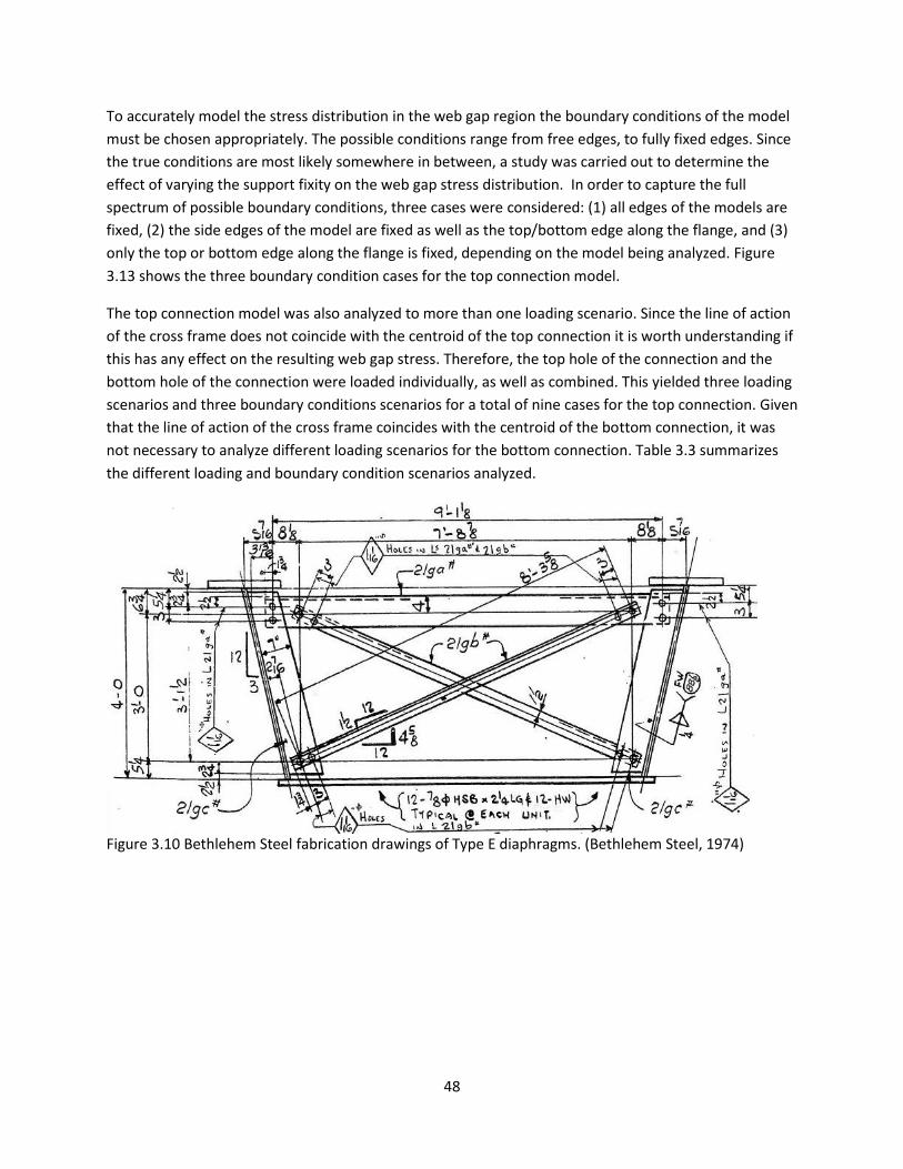
48

To accurately model the stress distribution in the web gap region the boundary conditions of the model

must be chosen appropriately. The possible conditions range from free edges, to fully fixed edges. Since

the true conditions are most likely somewhere in between, a study was carried out to determine the

effect of varying the support fixity on the web gap stress distribution. In order to capture the full

spectrum of possible boundary conditions, three cases were considered: (1) all edges of the models are

fixed, (2) the side edges of the model are fixed as well as the top/bottom edge along the flange, and (3)

only the top or bottom edge along the flange is fixed, depending on the model being analyzed. Figure

3.13 shows the three boundary condition cases for the top connection model.

The top connection model was also analyzed to more than one loading scenario. Since the line of action

of the cross frame does not coincide with the centroid of the top connection it is worth understanding if

this has any effect on the resulting web gap stress. Therefore, the top hole of the connection and the

bottom hole of the connection were loaded individually, as well as combined. This yielded three loading

scenarios and three boundary conditions scenarios for a total of nine cases for the top connection. Given

that the line of action of the cross frame coincides with the centroid of the bottom connection, it was

not necessary to analyze different loading scenarios for the bottom connection. Table 3.3 summarizes

the different loading and boundary condition scenarios analyzed.

Figure 3.10 Bethlehem Steel fabrication drawings of Type E diaphragms. (Bethlehem Steel, 1974)

49

Figure 3.11 Top connection model. Note higher mesh density in web gap region and bolt holes not aligned with the cross frame member.

Figure 3.12 Bottom connection model. Note higher mesh density in web gap region and bolt holes aligned with the cross frame member.

50

Figure 3.13 Boundary condition cases for the top connection model.

Table 3.3 Summary of loading and boundary condition cases

Model Loading Conditions Boundary Conditions

Bottom Connection Both holes loaded

All edges fixed

Bottom edge & sides fixed

Bottom edge fixed

Top Connection

Top hole loaded

All edges fixed

Top edge & sides fixed

Top edge fixed

Bottom hole loaded

All edges fixed


Top edge fixed

Both holes loaded

All edges fixed


Top edge fixed

Local Model Results

The FE results show the presence of a large stress gradient in the web gap region caused by the cross

frame forces. This stress gradient was present in all boundary condition cases and all loading scenarios

for the top connection model. Moreover, the results show that the stress concentration due to the cross

frame forces is highly localized to the web gap region and does not extend longitudinally far from the

connection plate along the web of the girder. Sample stress contour plots can be seen in Figure 3.14 to

Figure 3.16.

The results of the boundary condition analysis are summarized in Table 3.4. Results are presented for

the total load of 2.82 kips on the connection, and then normalized to a 1 kip total load. The choice of

boundary conditions significantly affects the stress distribution near the web gap for a given loading. For

the bottom connection model, the maximum nodal principal stress at the weld toe decreases as the

fixity around the edges increases. It ranges from a high of 13.7 ksi for just the bottom edge fixed, to a

51

low of 10.8 ksi for all edges fixed. For the top connection model with both holes loaded, the opposite is

true, although the variation with different support conditions is not as significant. The maximum

principal stress ranges from a low of 10.9 ksi for just the top edge fixed, to a high of 11.3 ksi for all edges

fixed. Furthermore, for the same total load, the stresses are in general higher in the bottom connection

plate than in the top connection plate.

One conclusion that can be drawn from the local model results is that for the same total load, the

maximum stress in the bottom connection is higher than in the top connection. Higher stresses at the

bottom connection would inevitably lead to more fatigue cracks at these locations. The 2007 AECOM

inspection report crack list confirms this finding; 75% of the cracks detected occurred at the bottom

connection detail. The full crack list from the 2007 inspection can be found in Kucz (2009). More of the

local model results can be found in Soto Fuentes (2011).

Figure 3.14 Bottom connection, bottom edge only fixed analysis results. Maximum principal stress concentrations are highly localized near web gap region.

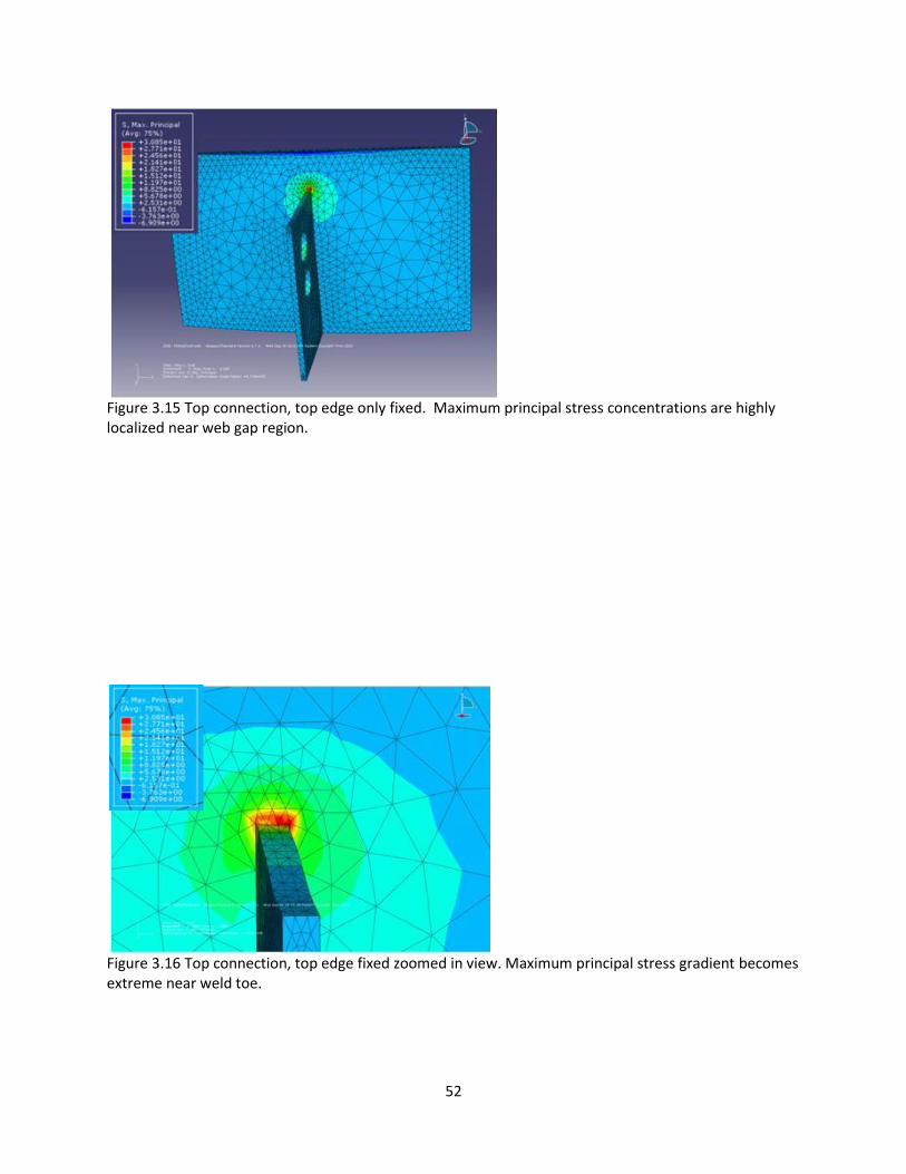
52

Figure 3.15 Top connection, top edge only fixed. Maximum principal stress concentrations are highly localized near web gap region.

Figure 3.16 Top connection, top edge fixed zoomed in view. Maximum principal stress gradient becomes extreme near weld toe.

53

Table 3.4 Boundary condition study results (all stresses in ksi)

Bottom Connection Plate

2.82 kip load Normalized to 1 kip load

Min Principal

Stress

Max Principal

Stress

Min Principal

Stress

Max Principal

Stress

Bottom Edge Fixed -6.12 38.82 -2.16 13.73

Bottom and Sides Fixed -6.79 34.44 -2.40 12.18

All Edges Fixed -6.87 30.44 -2.43 10.76

Top Connection Plate (both holes loaded)

2.82 kip load Normalized to 1 kip load

Min Principal

Stress

Max Principal

Stress

Min Principal

Stress

Max Principal

Stress

Top Edge Fixed -6.91 30.80 -2.44 10.89

Top and Sides Fixed -6.90 30.80 -2.44 10.89

All Edges Fixed -6.23 31.90 -2.20 11.28

54

4 Fatigue Analysis

4.1 Introduction

In this chapter, the FE models and in-service test results are used to conduct a fatigue analysis of the

viaduct. The goal of the analysis is to determine if the observed fatigue cracking is consistent with

expected behavior given the stress range and traffic loads, to determine if additional fatigue cracking

could be expected in the future, and to help guide the retrofit options, which are discussed in Chapter 5.

The analysis was carried in accordance with the AASHTO Manual for Condition Evaluation and Load and

Resistance Factor Rating (LRFR) of Highway Bridges (referred to here as Manual).

4.2 Estimating Remaining Life

Distortion-induced fatigue cracking at unstiffened web gaps has been widely documented to be

represented by a Category C Fatigue Detail. In this analysis, the Type E diaphragm web gaps were

considered a Category C detail (this was also based on recommendations made by DelDOT and the

consultant AECOM). Per Manual, the effective stress range at a fatigue prone detail is estimated as:

sefff R f (4.1)

in which sR is the stress range partial load factor, which for estimating mean fatigue life, whether based

on analysis or measured stresses, is taken to be equal to 1.0; and f is the measured stress range or

0.75 times the calculated stress range (which represents the live load factor for the fatigue limit state

and the design truck, as specified by AASHTO LRFD).

Details are only considered to be prone to fatigue if the net live load tensile stress exceeds the dead load

compressive stress. Since cracks have been observed in numerous connection details it can be assumed

that many of them do experience net tensile stresses due to the live loads.

A detail is said to have infinite fatigue life if

max TH

f F (4.2)

in which max

f is the maximum expected stress range, which can be taken to be equal to 2 times

eff

f , and TH

F is the constant amplitude fatigue threshold for the detail, as given in the AASHTO

LRFD specification. For a category C detail, 10TH

F ksi .

If equation (4.2) is not satisfied, then the detail has a finite fatigue life. The total fatigue life of a detail, in

years, is given by

55

3

365

Rf

SL eff

R AY

n ADTT f

(4.3)

in which

finite fatigue life in years

resistance factor that depends on the category detail and if the calculation

is to be done for minimum, evaluation, or mean fatigue life

lifetime average daily

f

R

SL

Y

R

ADTT

truck traffic in a single lane

number of stress cycles per truck

category detail constant

effective stress rangeeff

n

A

f

For a Category C detail and mean fatigue life, RR =1.3; 844 10A (AASHTO LRFD). The test results

(Chapter 2) showed that the details experience one cycle for each passage of the truck; therefore, 1n

. Substituting these values into (4.3) and simplifying yields

8 7

3 3

1.3 44 10 1.567 10

365f

SL eff SL eff

Y

ADTT f ADTT f

(4.4)

To estimate the fatigue life it remains to determine the stress range and the SLADTT (otherwise

referred to as the lifetime average daily truck traffic). The effective stress range can be estimated using

FE models, or from in-service measurements of the actual strains. The SLADTT can be estimated from

traffic count data provided by DelDOT, or also from the in-service measurements of the actual strains.

Estimates of the fatigue life were first made based on the results of the S10 model and ADT data

provided by DelDOT. Later, after the in-service monitoring was completed, estimates were made using

the field data in conjunction with the local FE connection model. The results of the two processes are

discussed below.

4.3 Global model estimate

Lifetime Average Daily Truck Traffic

The first step to determining the lifetime SLADTT is to determine the present day average daily truck

traffic ( PRADTT ) from data provided by the bridge owner. For the Newport Viaduct, DelDOT provided

an ADT estimate of 69,412 (northbound and southbound directions) for 2007, with 9% truck traffic. The

ADTT for both directions was therefore 6,247 in 2007. Assuming an equal distribution of trucks in both

directions (northbound and southbound), the ADTT for each direction was 3,124.

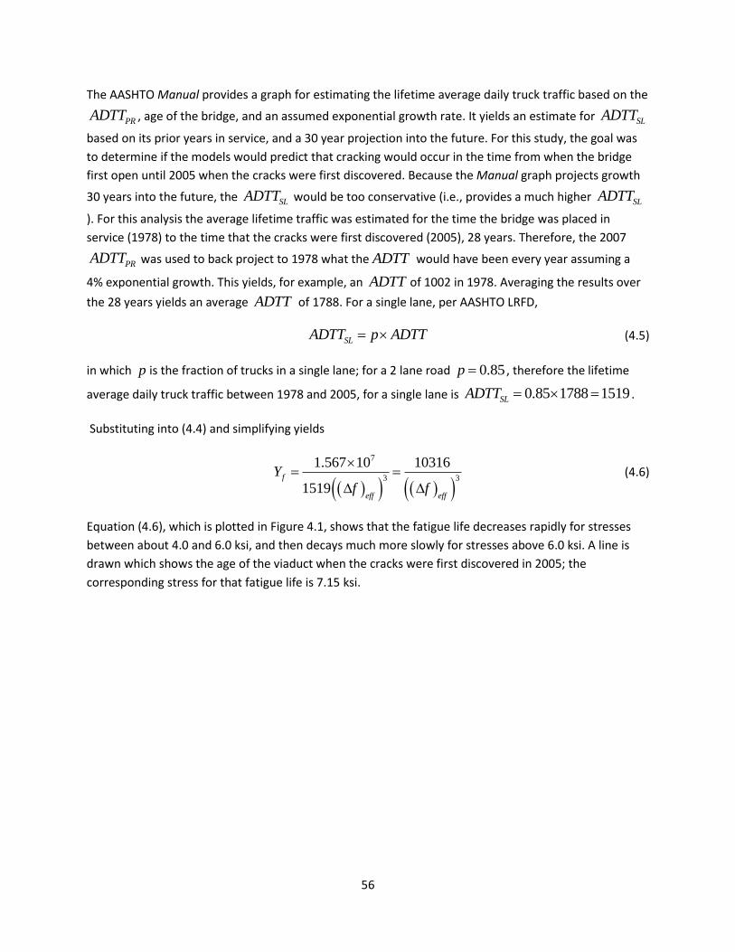
56

The AASHTO Manual provides a graph for estimating the lifetime average daily truck traffic based on the

PRADTT , age of the bridge, and an assumed exponential growth rate. It yields an estimate for SLADTT

based on its prior years in service, and a 30 year projection into the future. For this study, the goal was

to determine if the models would predict that cracking would occur in the time from when the bridge

first open until 2005 when the cracks were first discovered. Because the Manual graph projects growth

30 years into the future, the SLADTT would be too conservative (i.e., provides a much higher SLADTT

). For this analysis the average lifetime traffic was estimated for the time the bridge was placed in

service (1978) to the time that the cracks were first discovered (2005), 28 years. Therefore, the 2007

PRADTT was used to back project to 1978 what the ADTT would have been every year assuming a

4% exponential growth. This yields, for example, an ADTT of 1002 in 1978. Averaging the results over

the 28 years yields an average ADTT of 1788. For a single lane, per AASHTO LRFD,

SLADTT p ADTT (4.5)

in which p is the fraction of trucks in a single lane; for a 2 lane road 0.85p , therefore the lifetime

average daily truck traffic between 1978 and 2005, for a single lane is 0.85 1788 1519SLADTT .

Substituting into (4.4) and simplifying yields

7

3 3

1.567 10 10316

1519f

eff eff

Y

f f

(4.6)

Equation (4.6), which is plotted in Figure 4.1, shows that the fatigue life decreases rapidly for stresses

between about 4.0 and 6.0 ksi, and then decays much more slowly for stresses above 6.0 ksi. A line is

drawn which shows the age of the viaduct when the cracks were first discovered in 2005; the

corresponding stress for that fatigue life is 7.15 ksi.

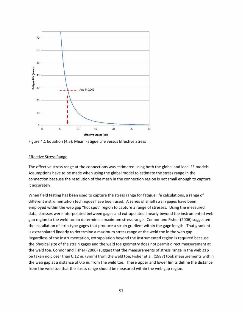
57

Figure 4.1 Equation (4.5): Mean Fatigue Life versus Effective Stress

Effective Stress Range

The effective stress range at the connections was estimated using both the global and local FE models.

Assumptions have to be made when using the global model to estimate the stress range in the

connection because the resolution of the mesh in the connection region is not small enough to capture

it accurately.

When field testing has been used to capture the stress range for fatigue life calculations, a range of

different instrumentation techniques have been used. A series of small strain gages have been

employed within the web gap “hot spot” region to capture a range of stresses. Using the measured

data, stresses were interpolated between gages and extrapolated linearly beyond the instrumented web

gap region to the weld toe to determine a maximum stress range. Connor and Fisher (2006) suggested

the installation of strip-type gages that produce a strain gradient within the gage length. That gradient

is extrapolated linearly to determine a maximum stress range at the weld toe in the web gap.

Regardless of the instrumentation, extrapolation beyond the instrumented region is required because

the physical size of the strain gages and the weld toe geometry does not permit direct measurement at

the weld toe. Connor and Fisher (2006) suggest that the measurements of stress range in the web gap

be taken no closer than 0.12 in. (3mm) from the weld toe; Fisher et al. (1987) took measurements within

the web gap at a distance of 0.5 in. from the weld toe. These upper and lower limits define the distance

from the weld toe that the stress range should be measured within the web gap region.

58

In cases in which FE modeling was used to predict stress ranges for distortion-induced fatigue, a refined

mesh at the detail of interest was required to produce an accurate FE model approximation of stress

(Roddis and Zhao, 2003; Jajich and Schultz, 2003). In the past, the mesh refinement was limited due to

computational resources. Advances in computing capacity and commercially available FE software has

enabled the refined mesh to be comprised of element sizes much smaller relative to the past. Roddis

and Zhao (2003) noted that as mesh density increases, infinitely large stresses are predicted by FE

approximations. They chose to select a lower bound mesh size of 0.16 in. (4.25mm) within the web gap

region. Jajich and Schultz (2003) confirmed that distortion-induced fatigue stresses in the web gap “hot

spot” region were mesh-dependent and attenuated rapidly; however, they relied on correlation to field

results to determine their stress range and thus avoided selecting an overly dense mesh.

Hobbacher (2009) described a method to quantify the “hot spot” stress that should be used in

conjunction with fatigue life calculations. In the method, FE model stress approximations are plotted as

a function of the distance from the weld toe. Typically the stresses become infinite as the distance from

the weld to decreases, consistent with Roddis and Zhao (2003) and Jajich and Schultz (2003). To account

for the asymptotic FE stresses, Hobbacher (2009) suggests a linear extrapolation to the weld toe using

FE stress approximations at a distance of 0.4t and 1.0t from the weld toe, where t is the thickness of the

welded attachment. The linear extrapolation avoids using an artificially high stress range with small

mesh sizes and an artificially low stress range with elemental approximations far from the weld toe.

In summary, Connor and Fisher (2006) established a lower bound field instrumentation position of 0.12

in from the weld toe. In FE model studies, Roddis and Zhao employed a lower bound FE mesh size of

0.16 in. to capture the stress range. Hobbacher (2009) used a linear extrapolation of the FE

approximations to capture a stress range at the “hot spot” location. In the fatigue analysis of the

Newport Viaduct, a range of the aforementioned methods were used to capture the stress range at the

Type E diaphragm web gap locations from the global span 10 model. The FE model was refined to

element sizes of 0.1 in. that represented the lower bound distance established by Connor and Fisher

(2006). The mesh size employed by Roddis and Zhao fell within this range. The stress ranges used for

fatigue life calculations were determined using 3 locations/methods: the FE approximation at an

element location represented by Connor and Fisher (2006) as a lower bound gage measurement

position (0.16 in. from weld toe), the FE approximation at an element location represented by Fisher et

al. (2006) as an upper bound gage measurement position (0.5 in. from weld toe), and the linear

extrapolation of the FE approximations described by Hobbacher (2009).

Since shell elements were used in the S10 model, out of plane stresses from the web elements were not

available. As an alternative, normal stresses in the connection plate perpendicular to the girder web (x-

direction) were used, as shown in Figure 4.2.

59

Figure 4.2 Direction of stress taken from global S10 model for fatigue evaluation

Figure 4.3 Typical contour plot of stresses in web and connection plate

A typical contour plot of the stresses in the web and connection plate for the S10 model is shown in

Figure 4.3. Table 4.1 shows the stress ranges obtained from the S10 model for all eight connections for

the three different methods. The stresses obtained a distance of 0.14 in. from the weld toe, and using

the linear interpolation from a bit further away (the Hobbacher (2009) method) are very comparable.

The stress range taken a distance of 0.56 in. from the weld toe is about half that of the other two

methods. Note also that half of the connections report a compressive stress range and the other half a

tensile stress range. Looking carefully at the deformed shape of the girder for the vehicle in different

positions, when the connection is in compression the girder web is deformed in such a way that the

60

outside face of the web would be in tension. While this location is not near the weld toe, and the

inspection did not reveal any initiation of cracks on the outside face of the web, the fatigue life was

calculated anyway for these areas, assuming the stress was tensile and not compressive.

Table 4.1 Stress range from global S10 model at all eight connections

Method Distance from weld toe (in)

Fatigue Detail Location

A B C D E F G H

1 Connor and

Fisher (2006) 0.14 12.1 -20.0 -14.5 18.8 -11.9 19.0 15.4 -20.2

2 Fisher et al.

(1987) 0.56 6.0 -7.2 -7.3 6.9 -5.9 7.0 7.7 -7.2

3 Hobbacher

(2009) Linear

extrapolation 11.8 -17.5 -14.2 16.5 -11.7 16.7 15.1 -17.6

Using the effective stresses in Table 4.1, the fatigue life of the connections was calculated and are listed

in Table 4.2. As one would expect, since the stresses are comparable, the estimates based on the

effective stress using the Connor and Fisher (2006) recommendation and the Hobbacher (2009)

recommendation are very similar. They range from under 1 year to 3 years. The estimates based on the

stresses obtained using the Fisher et al (1987) recommendation are much greater, and range from a low

of 10 years to a high of just under 23 years.

Table 4.2 Estimated fatigue life of the eight connections



A B C D E F G H

1 Connor and

Fisher (2006) 0.14 6 1 3 2 6 1 3 1

2 Fisher et al.

(1987) 0.56 47 28 27 32 49 30 22 27

3 Hobbacher

(2009) Linear

extrapolation 6 2 4 2 6 2 3 2

The fatigue life predicted by Method 1 and 3 appear lower than expected given the condition of the

fatigue cracks observed on the structure in interior box inspections. Specifically, the actual fatigue

cracks within the structure have been observed as actively propagating. Furthermore, a low percentage

of cracks (approximately 15% or less) have observable oxidation from being exposed to atmospheric

conditions over a long period of time. If the cracks had formed when predicted by Method 1 and 3, the

following situations would be expected: (1) all of the web gap regions would have been observed as

cracked in interior box inspections, (2) noticeable rust would be expected on unprotected, cracked

surfaces on a high percentage of cracked locations, and (3) cracked locations would have propagated to

some equilibrium or irreversible damage state in the time since cracking was predicted to occur. The

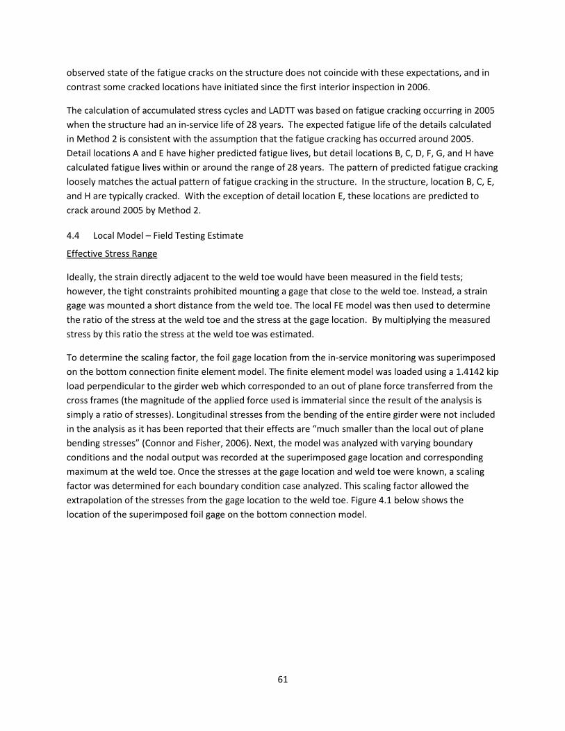
61

observed state of the fatigue cracks on the structure does not coincide with these expectations, and in

contrast some cracked locations have initiated since the first interior inspection in 2006.

The calculation of accumulated stress cycles and LADTT was based on fatigue cracking occurring in 2005

when the structure had an in-service life of 28 years. The expected fatigue life of the details calculated

in Method 2 is consistent with the assumption that the fatigue cracking has occurred around 2005.

Detail locations A and E have higher predicted fatigue lives, but detail locations B, C, D, F, G, and H have

calculated fatigue lives within or around the range of 28 years. The pattern of predicted fatigue cracking

loosely matches the actual pattern of fatigue cracking in the structure. In the structure, location B, C, E,

and H are typically cracked. With the exception of detail location E, these locations are predicted to

crack around 2005 by Method 2.

4.4 Local Model – Field Testing Estimate

Effective Stress Range

Ideally, the strain directly adjacent to the weld toe would have been measured in the field tests;

however, the tight constraints prohibited mounting a gage that close to the weld toe. Instead, a strain

gage was mounted a short distance from the weld toe. The local FE model was then used to determine

the ratio of the stress at the weld toe and the stress at the gage location. By multiplying the measured

stress by this ratio the stress at the weld toe was estimated.

To determine the scaling factor, the foil gage location from the in-service monitoring was superimposed

on the bottom connection finite element model. The finite element model was loaded using a 1.4142 kip

load perpendicular to the girder web which corresponded to an out of plane force transferred from the

cross frames (the magnitude of the applied force used is immaterial since the result of the analysis is

simply a ratio of stresses). Longitudinal stresses from the bending of the entire girder were not included

in the analysis as it has been reported that their effects are “much smaller than the local out of plane

bending stresses” (Connor and Fisher, 2006). Next, the model was analyzed with varying boundary

conditions and the nodal output was recorded at the superimposed gage location and corresponding

maximum at the weld toe. Once the stresses at the gage location and weld toe were known, a scaling

factor was determined for each boundary condition case analyzed. This scaling factor allowed the

extrapolation of the stresses from the gage location to the weld toe. Figure 4.1 below shows the

location of the superimposed foil gage on the bottom connection model.

62

Figure 4.4 Foil gage #1 field location superimposed on localized bottom connection model web gap

The finite element analysis results show that a very high stress gradient exists in the web gap region.

However, the foil gage installed in the web gap region only provides a single strain output obtained by

integrating strains over its entire length. To obtain a single strain value corresponding to the foil gage,

the output at three nodal points along the superimposed length of the foil gage were recorded and

averaged. The three nodal locations used corresponded to the top, middle and bottom of the

superimposed foil gage. Similarly to the boundary condition study carried out in Chapter 3 (see Table

3.4), scaling factors were determined for three sets of boundary conditions. The output of interest was

the vertical or Y-component of the maximum principal stress. Table 4.3 on the next page, summarizes

the y stress output at the superimposed foil gage location and corresponding weld toe maximum

stress.

63

Table 4.3 Stress at superimposed foil gage location and corresponding weld toe maximum stress, for varying boundary conditions

All fixed Bottom & Sides Fixed Bottom Fixed

Superimposed FG#1 Location (ksi)

2.40 2.12 1.77

σy at weld toe (ksi) 25.11 28.57 32.45

Scaling Factor 10.46 13.48 18.33

Given a variable amplitude loading in histogram form, Miner’s rule is used to calculate an “effective”

stress, which is given by

1/3

3

1

k

r i i

i

S f S

(4.7)

in which iS is the bin mid-width stress and if is the fraction of cycles in that range.

Vehicles weighing less than 20 kips have a very low probability of causing fatigue damage (Alampalli,

2006), thus, it becomes necessary to establish a minimum stress level for use in equation (4.7). The goal

is to eliminate those cycles that are not causing fatigue damage. Connor and Fisher (Connor and Fisher,

2006) and Zhou (Zhou, 2006) proposed using cutoff values, or minimum stresses, of 0.25CAFT and

0.50CAFT respectively. Given a constant amplitude fatigue threshold of 10.0 ksi for a Category C detail,

these proposed cutoff points would be 2.5 ksi and 5.0 ksi.

Difficulties arise when attempting to use a single factor of the CAFT as the cutoff value to calculate the

effective stress. Given the different scaling factors that arise from the various boundary conditions

analyzed, it is unclear which single value of stress at the weld toe is the most accurate. In other words,

the choice of boundary conditions significantly affects the magnitude of the stress at the weld toe thus

making it impossible to use a single CAFT factor as the cutoff point. For this reason, it became necessary

to calculate the effective stress for all boundary condition cases and their corresponding scaling factors.

Instead of using a single factor of the CAFT as the effective stress cutoff value, the mid-width value of

bins 2-7 of the Rainflow histogram (Table 3.3) was used. Table 4.3 on the next page summarizes the

effective stress calculation results.

Given the large variability in the calculated effective stresses at the weld toe, mean fatigue life was

calculated for each effective stress corresponding to the various boundary conditions.

64

Table 4.4 Effective Stress at weld toe for different cut-off (minimum) stresses

Bin Με

Cut-off

mid- bin

stress σMB

(ksi)

Total # of

Cycles

Cut-off stress at weld toe (ksi) Effective Stress at weld toe (ksi)

All fixed

(10.46* σMB )

Bottom &

Sides Fixed

(13.48* σMB )

Bottom Fixed

(18.33* σMB)

All

fixed

Bottom

& Sides

Fixed

Bottom

Fixed Average

2 5-10 0.22 1,546,673 2.28 2.93 3.99 3.54 4.56 6.21 4.77

3 10-15 0.36 304,556 3.79 4.88 6.64 5.62 7.24 9.85 7.57

4 15-20 0.51 102,143 5.31 6.84 9.30 7.50 9.66 13.14 10.10

5 20-25 0.65 42,758 6.83 8.79 11.96 9.28 11.95 16.30 12.51

6 25-30 0.80 20,309 8.34 10.74 14.62 11.00 14.17 19.28 14.82

7 30-35 0.94 10,608 9.86 12.70 17.28 12.65 16.28 22.16 17.03

65

Lifetime Average Daily Truck Traffic

Instead of using the present day PRADTT estimate provided by DelDOT to determine the SLADTT as

before, this analysis is based on the actual number of cycles recorded during the in-service monitoring.

These numbers are believed to be a better representation of the number of load cycles experienced by

the web gap detail as opposed to the bridge structure as a whole. The number of cycles for bins 2-7

(Table 4.4) was divided by 23, the length in days of the in-service monitoring period, to obtain an

average daily “truck” traffic count for 2011. As before, this present day PRADTT was then used to back

project what the ADTT was for every year the bridge was in service assuming a 4% exponential growth

rate. The SLADTT was then calculated as the average of those results between the time the bridge was

placed in service (1978), until the time the cracks were first discovered (2005). Table 4.4 shows a sample

of the estimated yearly ADTT and the SLADTT from 1978 to 2005.

Table 4.5 SLADTT estimates with 4% exponential growth rate.

Year Average Daily Truck Traffic (ADTT)

Bin 2 Bin 3 Bin 4 Bin 5 Bin 6 Bin 7

2011 67,247 13,242 4,441 1,859 883 461

2010 64,661 12,733 4,270 1,788 849 443

2009 62,174 12,243 4,106 1,719 816 426

2008 59,782 11,772 3,948 1,653 785 410

2007 57,483 11,319 3,796 1,589 755 394

2006 55,272 10,884 3,650 1,528 726 379

2005 53,146 10,465 3,510 1,469 698 364

… … … … … … …

1979 19,169 3,775 1,266 530 252 131

1978 18,432 3,630 1,217 510 242 126

1978 to 2005

SLADTT 32,893 6477 2172 909 432 225

The SLADTT estimates shown in Table 4.5 vary greatly. The values range from 32,893 for Bin 2 to 225

for Bin 7. These extreme values are not realistic representations of the actual SLADTT of the structure,

but are presented herein for completeness. Comparing the lifetime average estimates and the 2007

values, to the ADTT provided by DelDOT and the SLADTT calculated earlier from that value, it appears

that the results based on the bins 3, 4 and 5 seem to be the most realistic and reasonable. Note also that

when calculating the fatigue life the lane reduction factor (0.85) is not included since the number of

cycles is based on the actual measured strain at the connection, thus, any reduction it automatically

captured by the measured data.

66

The fatigue life was calculated for all boundary condition cases and all cut-off stress values. The results

are presented in Table 4.6. The predictions ranges from a low of 2 years to a high of 34 years. As

mentioned previously, some of the results can be excluded simply based on the very low or very high

SLADTT . This would be the case for bins 2, 6, and 7. The estimates for the “bottom fixed” boundary

condition case are all very low and can be discounted for the following reasons: (1) the results imply the

first cracks would have formed shortly after the bridge opened, i.e., in the 1980s. Had the fatigue cracks

formed in the 1980s, the in-depth inspection in 2005 would have discovered extensive corrosion at the

cracked locations and this was not the case. (2) the “bottom only fixed” boundary condition assumption

was clearly a lower bound case for the model; the other three edges are not free, but are constrained in

some manner. Fixing the bottom edge of the model and allowing all other edges to rotate/displace

freely does not approximate the true field conditions and leads to fatigue life estimates that are too low.

Eliminating these cases, and also those for bin 2, 6, and 7, yields the final results which are shown in

Table 4.7.

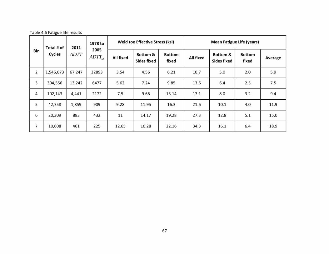
67

Table 4.6 Fatigue life results

Bin Total # of

Cycles

2011

ADTT

1978 to

2005

SLADTT

Weld toe Effective Stress (ksi) Mean Fatigue Life (years)

All fixed Bottom &

Sides fixed

Bottom

fixed All fixed

Bottom &

Sides fixed

Bottom

fixed Average

2 1,546,673 67,247 32893 3.54 4.56 6.21 10.7 5.0 2.0 5.9

3 304,556 13,242 6477 5.62 7.24 9.85 13.6 6.4 2.5 7.5

4 102,143 4,441 2172 7.5 9.66 13.14 17.1 8.0 3.2 9.4

5 42,758 1,859 909 9.28 11.95 16.3 21.6 10.1 4.0 11.9

6 20,309 883 432 11 14.17 19.28 27.3 12.8 5.1 15.0

7 10,608 461 225 12.65 16.28 22.16 34.3 16.1 6.4 18.9

68

Table 4.7 Fatigue life results

Bin Total # of

Cycles

2011

ADTT

1978 to

2005

SLADTT

Weld toe Effective Stress (ksi) Mean Fatigue Life (years)

All fixed Bottom &

Sides fixed

Bottom

fixed All fixed

Bottom &

Sides fixed Average

3 304,556 13,242 6477 5.62 7.24 9.85 13.6 6.4 10.0

4 102,143 4,441 2172 7.5 9.66 13.14 17.1 8.0 12.6

5 42,758 1,859 909 9.28 11.95 16.3 21.6 10.1 15.8

69

5 Retrofit Options

5.1 Introduction

After reviewing the various methods used to retrofit details prone to distortion induced fatigue cracking,

three options were selected for analysis through refined finite element modeling. Span 15 exhibited

only minimal cracking and span 10 had significant cracking; therefore, it was decided to perform the

retrofit analysis using the model for span 10 (details and model information for span 10 were discussed

in Chapter 3). To determine the effectiveness of each retrofit, the mesh was refined at the boundaries

between the connection plates and the webs for each web gap. Each model was then loaded with a

fatigue truck and local stresses from the model with the refined mesh were recorded. These local

stresses were then used in fatigue life calculations.

5.2 Retrofit Options

Three different retrofit options were investigated for the project: (1) positive attachment between the

connection plate and the girder flanges, (2) lengthening of the web gaps by creating a slot between the

connection plate and web at both the top and bottom of the connection plates, and (3) removal of the

diagonal members in diaphragm type E. Each is described in more detail below.

Positive Attachment

To create positive attachment, Fisher and Keating (1989) recommend using plates with a minimum

thickness of 3/4 in and to avoid field welding if possible. The ideal positive attachment retrofit would

therefore be bolted to both the connection plate and the flanges. To create such an attachment, either

a WT section or angle is needed. For this study, a WT section was chosen so that it could be bolted to

the flange on both sides of the connection plate.

In order to get a section with a stem deep enough to allow for the recommended 4 high strength bolts

per shear plane, a minimum depth of 12 in. was selected. The lightest section to satisfy this criteria and

also has a stem thickness of at least 3/4 in. is a WT 12 x 88. This has a flange width of 12-7/8 in. which

should be sufficient to allow for 2 bolts on each side of the connection plate. It has a thickness of 1.34

in. which exceeds the minimum specified by Fisher, but is thin enough to fit in the gap between the

plate and the flange. Although the sloped web of the girder would require a specially cut section, it was

modeled as adjacent to the web and flanges as described later on. A sketch of the attachment is shown

in Figure 5.1.

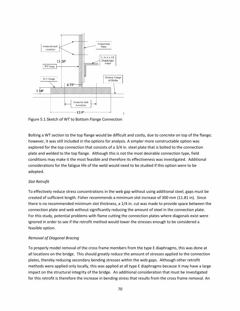
70

Figure 5.1 Sketch of WT to Bottom Flange Connection Bolting a WT section to the top flange would be difficult and costly, due to concrete on top of the flange;

however, it was still included in the options for analysis. A simpler more constructable option was

explored for the top connection that consists of a 3/4 in. steel plate that is bolted to the connection

plate and welded to the top flange. Although this is not the most desirable connection type, field

conditions may make it the most feasible and therefore its effectiveness was investigated. Additional

considerations for the fatigue life of the weld would need to be studied if this option were to be

adopted.

Slot Retrofit

To effectively reduce stress concentrations in the web gap without using additional steel, gaps must be

created of sufficient length. Fisher recommends a minimum slot increase of 300 mm (11.81 in). Since

there is no recommended minimum slot thickness, a 1/4 in. cut was made to provide space between the

connection plate and web without significantly reducing the amount of steel in the connection plate.

For this study, potential problems with flame cutting the connection plates where diagonals exist were

ignored in order to see if the retrofit method would lower the stresses enough to be considered a

feasible option.

Removal of Diagonal Bracing

To properly model removal of the cross frame members from the type E diaphragms, this was done at

all locations on the bridge. This should greatly reduce the amount of stresses applied to the connection

plates, thereby reducing secondary bending stresses within the web gaps. Although other retrofit

methods were applied only locally, this was applied at all type E diaphragms because it may have a large

impact on the structural integrity of the bridge. An additional consideration that must be investigated

for this retrofit is therefore the increase in bending stress that results from the cross frame removal. An

71

additional retrofit possibility would be loosening the bolts on the diagonal members, but to model this

would be no different than removing the members completely, thus was not considered separately.

5.3 Modeling the retrofits

To accurately capture the stress in the web gap, the global model for span 10 was remeshed at the web

gap of one representative cross frame in the region of the connection plate to web connections. The

cross frame selected is the same cross frame location that was instrumented during the live load

diagnostic test of span 10. The model was remeshed in a way to ensure that adjacent elements still

shared coincident nodes. By using minimally distorted quadrilateral elements, results will not be

adversely affected by the refined mesh. The refined mesh was first created for the case of existing field

conditions with no retrofits. An example of the finer mesh is shown in Figure 5.2.

Figure 5.2 Remesh of Original Model on Web and Connection Plate Modeling the Positive attachment

The refined mesh from the connection plates was also used to model the stem of the WT acting as the

positive attachment between the connection plate and the flanges. This stem is offset from the

connection plate and connected using rigid links. Since the meshes are the same size, it was possible to

link the nodes of all the elements, thus creating a completely rigid connection. However, since the

actual field connection would only be made using several bolts, the rigidity of which is questionable,

several different methods were used to model the connection to replicate upper and lower bound

stiffnesses of the connection. For the upper bound, links were placed at each node. To represent the

use of 4 bolts, 4 links in each shear plane were used for the lower bound. Two intermediate models

were also created, with varying number of nodal links. They will be described in detail in the results

section.

72

Figure 5.3 Model showing WT positive attachment at bottom flange The WT flange was modeled in a similar manner, however because there was no remeshing of the girder

flanges, the element size of the flanges was larger and constant. These were connected to the flanges

using rigid links, again with an upper and lower bound for comparison. Figure 5.3 shows a model of the

typical positive attachment of a WT to the bottom flange of a girder. The model for the top plate

attachment is similar to that of the stem of the WT, except for the fact that it is connected directly to

the top flange to represent the weld. Four rigid links were used in order to connect the plate to the top

flange. The refined mesh was used to create plate elements where they are adjacent to the connection

plate. An image of the typical modeled top flange tab connection is shown in Figure 5.4.

Figure 5.4 Model showing positive top flange connection

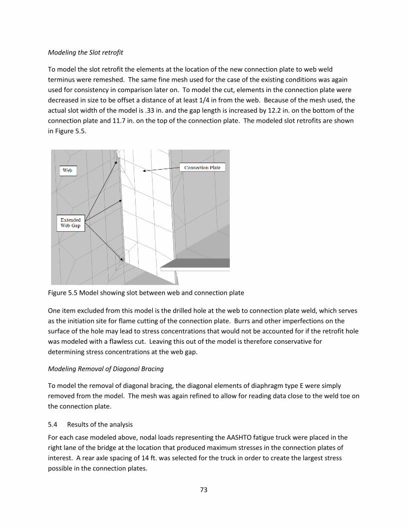
73

Modeling the Slot retrofit

To model the slot retrofit the elements at the location of the new connection plate to web weld

terminus were remeshed. The same fine mesh used for the case of the existing conditions was again

used for consistency in comparison later on. To model the cut, elements in the connection plate were

decreased in size to be offset a distance of at least 1/4 in from the web. Because of the mesh used, the

actual slot width of the model is .33 in. and the gap length is increased by 12.2 in. on the bottom of the

connection plate and 11.7 in. on the top of the connection plate. The modeled slot retrofits are shown

in Figure 5.5.

Figure 5.5 Model showing slot between web and connection plate One item excluded from this model is the drilled hole at the web to connection plate weld, which serves

as the initiation site for flame cutting of the connection plate. Burrs and other imperfections on the

surface of the hole may lead to stress concentrations that would not be accounted for if the retrofit hole

was modeled with a flawless cut. Leaving this out of the model is therefore conservative for

determining stress concentrations at the web gap.

Modeling Removal of Diagonal Bracing

To model the removal of diagonal bracing, the diagonal elements of diaphragm type E were simply

removed from the model. The mesh was again refined to allow for reading data close to the weld toe on

the connection plate.

5.4 Results of the analysis

For each case modeled above, nodal loads representing the AASHTO fatigue truck were placed in the

right lane of the bridge at the location that produced maximum stresses in the connection plates of

interest. A rear axle spacing of 14 ft. was selected for the truck in order to create the largest stress

possible in the connection plates.

74

In order to capture the stresses in the web gap near the weld tow, stresses in the connection plate were

recorded. Stresses from the connection plate had to be used because the model was made using shell

elements. Since the connection plates are oriented perpendicular to the web, the stresses transmitted

through these elements should be the same as the stresses that are seen at the weld toe. The stress at

the weld toe was determined using three different methods. Fisher measured gap stresses 0.12 in. from

the weld toe in 2006 and Fisher’s method from 1991 measured stresses 0.5 in from the weld toe. In

addition to using stresses from existing elements, extrapolation methods have also been used to

approximate stresses at the weld toe locations. To determine stresses in this manner, elements 3 and 4

were used to create a linear extrapolation and the stress where this intersected the vertical axis was

used as the stress at the weld toe. The stress values extracted from these elements were used as the

stress range in determining the remaining fatigue life of the bridge.

Original model (no retrofit)

Results of the remeshed model with no retrofits are presented in Table 5.1. The horizontal distance of

the centroid of the element to the weld toe is shown in the left column, and stresses are reported at

each web gap location. The sharp increases in stress as the elements get closer to the weld toe are

apparent. The rows highlighted in gray are the elements used directly for fatigue life calculation. The

3rd and 4th rows are the elements used to extrapolate the stress at the weld toe for the third method of

calculating fatigue life.

Table 5.1 Original Model Stresses for Refined Mesh

Distance to weld (in)

Stress (ksi) at Gap Location

A B C D E F G H

0.046875 17.43 -33.45 -20.97 31.17 -17.28 31.52 22.18 -33.73

0.140625 12.08 -20.02 -14.52 18.80 -11.94 19.05 15.38 -20.16

0.28125 8.94 -12.33 -10.75 11.66 -8.83 11.84 11.40 -12.41

0.5625 6.04 -7.18 -7.26 6.86 -5.94 6.98 7.72 -7.22

1.125 3.72 -3.28 -4.47 3.18 -3.63 3.25 4.77 -3.29

2.25 2.22 -2.45 -2.66 2.39 -2.14 2.43 2.85 -2.48

4.5 1.37 -1.57 -1.64 1.53 -1.32 1.55 1.76 -1.59

Stresses for these elements and the extrapolated values that were used in fatigue calculations are

shown in Table 5.2. Results for remaining fatigue life for the rest of the models will be saved for the end

of the chapter, but are presented here to detail the method used in the procedure.

Table 5.2 Expected Fatigue Life for Original Model

Label Location/



A B C D

Stre

ss

Ran

ge(

ksi)

Method 1 Connor and

Fisher (2006) 0.14 12.1 -20.0 -14.5 18.8

75

Method 2 Fisher et al.

(1987) 0.56 6.0 -7.2 -7.3 6.9

Method 3 Hobbacher

(2009) Linear

extrapolation 11.8 -17.5 -14.2 16.5

Fati

gue

Life

(yr

s)

Method 1 Connor and

Fisher (2006) 0.14 6 1 3 2

Method 2 Fisher et al.

(1987) 0.56 47 28 27 32

Method 3 Hobbacher

(2009) Linear

extrapolation 6 2 4 2

Positive attachment

The first case to be reported is the use of WT sections at both the top and bottom ends of connection

plates. To effectively connect the WT sections to both the connection plates and flanges, assumptions

had to be made. The shell elements required using rigid links between nodes to make these

connections. As mentioned before, both an upper and lower bound for the number of rigid links was

modeled. The lower bound case (Case A) has 4 links in each shear plane, representing the 4 bolts per

plane recommended by Fisher. The upper bound case (Case D) has links at each of the WT nodes,

excluding the elements in the remeshed region. Two additional intermediate models used 6 links

connecting the WT section to the flanges with a variable number of links on the top connection plate:

Case B has 4 links and Case C has 6 links. For both of these cases, the bottom of the connection plate is

connected to the WT with 4 links. Although each of these models differs slightly, they are all modeling

the positive connection with WT’s at both the top and bottom of each connection plate within cross

frame 2. A summary of the resulting stresses at the elements of interest is presented in Table 5.3.

Table 5.3 Stress Results for Positive Attachment with WT’s

Distance from weld toe (in)


A B C D E F G H

Stress Range (ksi)

Case A 4 Links Per Plane

0.14 5.0 -6.2 -6.8 5.5 -4.6 5.5 7.4 -7.0

0.56 2.5 -2.3 -3.4 2.1 -2.3 2.2 3.7 -2.4

Extrapolation 4.9 -4.8 -6.7 4.3 -4.5 4.2 7.2 5.4

Case B 4 Links on Connection Plate, 6 Links Per Flange

0.14 2.5 -4.3 -3.8 4.2 -2.4 4.2 4.3 -4.9

0.56 1.2 -1.8 -1.9 1.8 -1.2 1.8 2.2 -1.9

Extrapolation 2.4 -3.3 -3.7 3.3 -2.4 3.2 4.2 -3.8

76

Case C 6 Links on Connection Plate, 6 Links Per Flange

0.14 1.3 -4.4 -2.4 4.3 -1.1 4.3 2.6 -5.0

0.56 0.6 -1.8 -1.1 1.8 -0.5 1.9 1.2 -2.0

Extrapolation 1.2 -3.3 -2.2 3.3 -1.1 3.3 2.5 -3.8

Case D Links at Every Node (Except Remesh)

0.14 1.0 -2.2 -1.8 2.1 -0.9 2.1 2.0 -2.6

0.56 0.4 -0.5 -0.7 0.5 -0.4 0.6 0.8 -0.6

Extrapolation 0.9 -1.8 -1.7 1.7 -0.8 1.7 1.8 -2.1

It can be seen that the better the connection the greater the reduction in stress at the web gap. Table

5.4 presents the percent reduction in stress for each of the cases of positive WT attachment relative to

the original model. The reduction ranges from a low of 52% to a high of 94%; the actual reduction would

most likely fall somewhere in between. The effectiveness of this connection will depend on the

tightness of the WT to both the connection plate and flange members of the bridge. If this retrofit

method is chosen, sufficient clamping force needs to be provided via the bolts to optimize its

effectiveness.

Table 5.4 Percent Reduction in Stress Range for WT Positive Attachment



A B C D E F G H

Reduction In Stress Range (%)

Case A 4 Links Per Plane

0.14 59 69 53 71 62 71 52 65

0.56 59 69 54 69 62 69 52 66

Extrapolation 59 73 53 74 62 75 52 69

Case B 4 Links on Connection Plate, 6 Links Per Flange

0.14 79 78 73 77 80 78 72 76

0.56 80 75 74 74 80 74 72 73

Extrapolation 80 81 74 80 80 81 72 79

Case C 6 Links on Connection Plate, 6 Links Per Flange

0.14 89 78 84 77 91 78 83 75

0.56 90 75 85 74 91 73 84 73

Extrapolation 90 81 84 80 91 80 84 78

Case D Links at Every Node (Except Remesh)

0.14 91 89 87 89 93 89 87 87

0.56 93 94 90 93 94 92 90 92

Extrapolation 92 90 88 90 93 90 88 88

77

These values confirm that the amount of connectivity between elements strongly influences the

effectiveness of the retrofit. For the comparison of this type of retrofit to others, we will assume that

the actual retrofit will act somewhere between the upper and lower bounds of connectivity. This

assumption comes from the fact that although only the bolts will actually be connecting the members,

the tightness will be sufficient to cause the members to interact in a near slip-critical manner.

Similar results are presented in Table 5.5 for the case where the WT section is on the bottom flange and

a steel plate is used to provide positive attachment at the top. Upper and lower bond connectivity

options were modeled once again.

Table 5.5 Stress Results for Positive Attachment with WT’s at Bottom Flange and Plates at Top Flange



A B C D E F G H

Stress Range (ksi)

Case A 4 Links Per Plane, Weld at Top

0.14 2.6 -6.5 -4.0 5.8 -2.6 5.7 4.7 -7.2

0.56 1.3 -2.3 -2.0 2.2 -1.3 2.2 2.4 -2.5

Extrapolation 2.6 -5.0 -3.9 4.6 -2.5 4.4 4.6 -5.6

Case B Links at Every Node (Except Remesh)

0.14 1.1 -2.1 2.0 2.0 -1.0 2.0 2.1 -2.5

0.56 0.5 -0.4 -0.9 0.5 -0.5 0.5 0.9 -0.5

Extrapolation 1.0 -1.7 -1.9 1.7 -1.0 1.7 1.9 -2.0

For the web gaps located near the bottom of connection plates, the stresses are very similar to those for

the previous case. Web gap stresses at the top flange are actually lower than in the case of WT

connections for the case with 4 links however. This is due to the modeling of the welded connection

with 4 rigid links at the end of the plate. This allows for no rotation of the plate, and may therefore be

under conservative for this case. This is not viewed as a significant view in the case of the WT

connections because the flange is attached on either side of the plate and will likely be more resistant to

such rotation. Table 5.6 shows the percentage of reduction in stress from the original model. The

reduction ranges from a low of 66% to a high of 93%, very comparable to the previous case.

Table 5.6 Percent Reduction in Stress Range for WT’s at Bottom Flange and Plates at Top Flange



A B C D E F G H


Case A 4 Links Per Plane, Weld at Top

0.14 78 68 72 69 79 70 69 64

0.56 78 67 73 68 79 68 69 66

Extrapolation 78 71 73 72 79 74 70 68

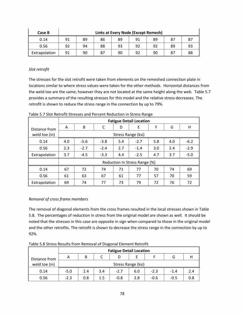
78

Case B Links at Every Node (Except Remesh)

0.14 91 89 86 89 91 89 87 87

0.56 92 94 88 93 92 92 89 93

Extrapolation 91 90 87 90 92 90 87 88

Slot retrofit

The stresses for the slot retrofit were taken from elements on the remeshed connection plate in

locations similar to where stress values were taken for the other methods. Horizontal distances from

the weld toe are the same; however they are not located at the same height along the web. Table 5.7

provides a summary of the resulting stresses for this model and the relative stress decreases. The

retrofit is shown to reduce the stress range in the connection by up to 79%.

Table 5.7 Slot Retrofit Stresses and Percent Reduction in Stress Range



A B C D E F G H

Stress Range (ksi)

0.14 4.0 -5.6 -3.8 5.4 -2.7 5.8 4.0 -6.2

0.56 2.3 -2.7 -2.4 2.7 -1.4 3.0 2.4 -2.9

Extrapolation 3.7 -4.5 -3.3 4.4 -2.5 4.7 3.7 -5.0


0.14 67 72 74 71 77 70 74 69

0.56 61 63 67 61 77 57 70 59

Extrapolation 69 74 77 73 79 72 76 72

Removal of cross frame members

The removal of diagonal elements from the cross frames resulted in the local stresses shown in Table

5.8. The percentages of reduction in stress from the original model are shown as well. It should be

noted that the stresses in this case are opposite in sign when compared to those in the original model

and the other retrofits. The retrofit is shown to decrease the stress range in the connection by up to

92%.

Table 5.8 Stress Results from Removal of Diagonal Element Retrofit



A B C D E F G H

Stress Range (ksi)

0.14 -5.0 2.4 3.4 -2.7 6.0 -2.3 -1.4 2.4

0.56 -2.3 0.8 1.5 -0.8 2.8 -0.6 -0.5 0.8

79

Extrapolation -4.9 2.1 3.3 -2.3 5.9 -2.0 -1.3 2.2

Reduction in Stress Range (%)

0.14 59 88 77 86 50 88 91 88

0.56 62 89 79 89 52 92 94 89

Extrapolation 59 88 77 86 50 88 91 87

5.5 Estimated fatigue life of retrofitted designs

Each of the retrofit methods selected for analysis significantly reduced the stresses in the web gaps. The

average decreases in stress for each modeled retrofit type are shown in Table 6 9. The upper bound for

both of the positive attachment methods are the most effective retrofits for reducing the stress in the

web gaps. As discussed before, these may be reducing the stress more than would actually occur in the

field, particularly in the case of the plate connections to the top flange. However, we shall assume that

the actual retrofit will act closer to the upper bound than the lower bound because tightness of the

bolts will provide better member interaction than simply connecting 4 points.

The stresses found at each location were used for determining the fatigue life of the bridge. Several

assumptions were made in adopting this procedure for the retrofits. The AASHTO category C detail was

used in each case. This detail should remain the same for both the removal of diaphragm cross frames

and the slot retrofits. However, the creation of positive attachment may result in a different fatigue

category. The reason that the type C detail was also used in this case is that the stresses of importance

are still within the web gap. Since the attachments are made to the connection plates and flanges, and

not the web itself it is considered to act in a similar manner. The fatigue life for each retrofit type at all

gap locations is presented in Table 6 10. The fatigue life is considered to be infinite if the stress range is

below the limiting stress range for the detail, which for category C is 4.4 ksi. This is represented in the

table by I.R.L., which stands for Infinite Remaining Life. The effectiveness of the retrofits is quite

apparent for each case. The method proposed by Fisher et al. best models the bridge with its current

cracking conditions. Using this method to measure stress 0.56 in. from the weld, all of the retrofits

result in infinite life.

Table 5.9 Summary of Stress Range Reductions from retrofit designs

Retrofit Method Average % Stress Reduction

Positive Attachment with WT

Case A 63

Case B 77

Case C 82

Case D 90

Positive Attachment with WT at

Bottom Flange and Plate at Top

Flange

Case A 72

Case B 90

Removal of Diagonals - 79

12 in. Slot Retrofit - 70

81

Table 5.10 Expected fatigue life for original model and retrofit


Fatigue Life (yrs) at Detail Location

A B C D E F G H

Original Model

0.14 6 1 3 2 6 1 3 1

0.56 47 28 27 32 49 30 22 27

Extrapolation 6 2 4 2 6 2 3 2

Positive Attachment with WT's, 4 Links Per Connection Plate and Flange

0.14 83 44 33 62 106 63 26 30

0.56 I.R.L. I.R.L. I.R.L. I.R.L. I.R.L. I.R.L. I.R.L. I.R.L.

Extrapolation 88 94 35 I.R.L. 113 I.R.L. 27 64

Positive Attachment with WT's, 4 Links on Connection Plate, 6 Per Flange

0.14 I.R.L. I.R.L. I.R.L. I.R.L. I.R.L. I.R.L. I.R.L. 86


Extrapolation I.R.L. I.R.L. I.R.L. I.R.L. I.R.L. I.R.L. I.R.L. I.R.L.

Positive Attachment with WT's, 6 Links on Connection Plates and Flanges

0.14 I.R.L. I.R.L. I.R.L. I.R.L. I.R.L. I.R.L. I.R.L. 83



Positive Attachment with WT's, Links at every Node (Except Remesh)




4 Links Per Plane, Welded Tab at Top

0.14 I.R.L. 38 I.R.L. 51 I.R.L. 56 98 27


Extrapolation I.R.L. 81 I.R.L. 107 I.R.L. 120 107 57

WT Bottom, Tab Top - Links at Every Node (Except Remesh)




Diagonals Removed

0.14 84 I.R.L. I.R.L. I.R.L. 48 I.R.L. I.R.L. I.R.L.


Extrapolation 89 I.R.L. I.R.L. I.R.L. 51 I.R.L. I.R.L. I.R.L.

12 in. Slot Retrofit

0.14 I.R.L. 58 I.R.L. 66 I.R.L. 53 I.R.L. 43


Extrapolation I.R.L. 110 I.R.L. I.R.L. I.R.L. 101 I.R.L. 82

82

6 Summary and Conclusions

A research project was undertaken to investigate the problem of fatigue cracking in the steel tub girders

of the Rt. 141 Newport Viaduct, located in New Castle Co., Delaware. The 19 span viaduct was built in

1978 and carries a high level of traffic. The first internal inspection of the viaduct, conducted in 2005,

discovered a large number of fatigue cracks in the web gap region where the diaphragm connection

plate is welded to the girder web. The fatigue cracks were likely caused by distortion induced

deformation of the region. The research project involved field testing (a controlled load test and in-

service monitoring), numerical modeling (global finite element models of two sections, and local models

of the connection region), fatigue evaluation, and the evaluation of several different retrofit options.

The results of this multi-year investigation are summarized in detail in three master’s thesis (Kusc, 2009;

Quigley, 2009; Soto Fuentes 2011). The key conclusions from the investigation are the following:

1. Controlled load tests were conducted of spans 10 and 15. For each one, strain transducers were

mounted to the flanges, web, and cross frame members at three different diaphragm locations.

Strains were recorded as two 53 kip loaded trucks crossed the bridge. For span 10, the absolute

maximum stress recorded was 1.87 ksi in the bottom flange; the absolute minimum stress

recorded was -0.61 ksi in a cross frame member. For span 15, the absolute maximum stress

recorded was 2.68 ksi in the bottom flange; the absolute minimum stress recorded was -0.75 ksi,

also in the bottom flange.

2. In-service monitoring was conducted in span 10 to gather data due to the site-specific traffic for

the fatigue evaluation. Eight strain gages/transducers were installed around the diaphragm and

in the web gap region. The strains were recorded 24/7 for 23 days, and processed automatically

using the Rainflow algorithm. The system ran continuously off of two large marine grade 12 volt

batteries; the system was remotely accessible for 2 hours a day through a cellular modem. The

largest number of cycles, and the cycles of highest magnitude, were experienced in the bottom

web gap region and the web next to the connection plate at the bottom of the web.

3. Global, high-fidelity, finite element models were created of spans 9 to 11, and spans 12 to 16, of

the viaduct. The global models represented the steel tub girders and the concrete composite

deck in great detail, using primarily shell type elements. Beam elements were used to model the

cross frame members, rigid links were used to connect the girder to the deck and the parapet to

the deck, and appropriate boundary conditions were specified at the bearing locations. Results

of the controlled load test were used to calibrate the models. A sensitivity study showed that

moderate changes to the transverse position of the truck, concrete modulus, and connectivity of

the parapet did not result in better agreement uniformly, therefore, no significant changes were

made to the models. The agreement between the model and test results for the global member

behavior were sufficiently accurate to use the models for the subsequent fatigue evaluation and

retrofit study.

83

4. Local 3D finite element models of the connection were created, one for the top connection and

for the bottom connection. The models were loaded through the bolt holes of the connection,

as they would be in field. The results show a very localized, but high stress gradient in the web

gap region where the fatigue cracks occurred, consistent with what was found in the field

inspection. Analyses were conducted to study the effect of the boundary conditions on the

connection stresses: the bottom connection region was found to be more sensitive to the choice

of boundary conditions than the top connection. Furthermore, for the same loading, the bottom

connection had higher stresses in the web gap than the top connection. This finding is also

consistent with the inspection results that showed the majority of the cracks occurred in the

bottom connection.

5. A fatigue evaluation was conducted using the global finite element models to see if the fatigue

life was consistent with the observed cracking. The lifetime average daily truck traffic was

calculated based on the ADT measured by DelDOT in 2007. The stress range at the weld toe was

determined using three different methods as reported in the literature. Two of the methods

predicted cracking would occur within a few years of the bridge opening, which does not seem

plausible given other data obtained about the condition of the cracked regions. The third

method predicted cracking would have occurred within a time frame that is consistent with the

observed behavior. Regardless of the method, all resulted in life evaluations that predicted

cracking would occur.

6. The fatigue evaluation was also conducted using the results of the in-service monitoring. This

required calculating the effective stress at the weld toe. This was done by calculating the

effective stress in the web gap region where the strain gage was located, and transferring this to

the weld toe using the results of the local finite element model. The lifetime average daily truck

traffic was determined using the histograms from the rainflow data. Based on this analysis the

connections were found to have a mean fatigue life of between 10 and 16 years, which is quite

consistent with the observed behavior.

7. The global finite element model of span 10 was used to investigate several different retrofit

options for the repair of the connections. Three different options were considered: provide

positive attachment of the connection plate to the flange; create a slot between the connection

plate and the web; and remove the diagonal bracing. All of the methods resulted in a decrease

in the stress at the connection, with the reduction ranging from 60 to 90% from the original

design. In this case, all of the options would appear to be acceptable. A final decision would,

however, also depend on the constructability of the repair and the impact on the other design

criteria for the bridge.

84

7 References

AASHTO. (1990). Guide Specifications for Fatigue Evaluation of Existing Steel Bridges American

Association of State Highway and Transportation Officials, Washington D.C.

ABAQUS. (2008). ABAQUS Analysis User’s Manual, Pawtucket, R.I.

AECOM. (2007). “2006 Initial Interior Box Inspection Report.” Horsham, Pa.

Alampalli, S. and Lund R. (2006). “Estimating Fatigue Life of Bridge Components Using Measured

Strains.” Journal of Bridge Engineering, 11(6), 725-736.

Berglund, Evan M., and Arturo E. Schultz. (2006). “Girder Differential Deflection and Distortion-Induced

Fatigue in Skewed Steel Bridges.” Journal of Bridge Engineering Mar. / Apr., 169-177.

Bridge Diagnostics Inc. (2006). Strain Transducer For Structural Testing. 15 Jan. 2009. <

http://www.bridgetest.com/products/strain_transducers.html>

Connor, Robert, and John W. Fisher. (2006). “Identifying Effective and Ineffective Retrofits for

Distortion Fatigue Cracking in Steel Bridges Using Field Instrumentation.” Journal of Bridge

Engineering Nov. / Dec., 745-752.

DelDOT. (2007). “DelDOT’s Priority Bridges” 3 Feb.

2009.http://www.transportation1.org/BridgeReport/docs/DelDOT%20Priority%20Bridges.pdf

DelDOT. (1974). Structural Drawings for Newport Viaduct, Bridge 1-501. Prepared by Gannet

Fleming Corddry & Carpenter Inc.

Fisher, John W. and Peter Keating. (1989) “Distortion-Induced Fatigue Cracking of Bridge Details

with Web Gaps.” Journal of Constructional Steel Research 12, 215-228.

Fisher, John W., Dennis R. Mertz., and Kuang-Chong Wu. (1982). “Displacement-Induced Fatigue

Cracking of a Box Girder Bridge.” IABSE Reports, 71-76.

http://www.transportation1.org/BridgeReport/docs/DelDOT%20Priority%20Bridges.pdf

85

Fisher, J. W., Yen, B. T., and Wagner, D. C. (1987). “Review of field measurements for distortion-induced

fatigue cracking in steel bridges.” Transportation Research Record, 1118, 49-55.

Fisher, John W., et al. (1990). “Distortion-Induced Fatigue Cracking in Steel Bridges.” National

Cooperative Highway Research Program Report 336 Transportation Research Board,

Washington D.C. Dec

Google Maps. (2009). 3 Apr. < http://maps.google.com>

Hobbacher, A.F. (2009) “The New IIW Recommendations for Fatigue Assessment of Welded Joints and

Components – A Comprehensive Code Recently Updated.” International Journal of Fatigue 31.

50-59.

Jajich, D., and A. E. Schultz. (2003). “Measurement and Analysis of Distortion- Induced Fatigue in

Multigirder Steel Bridges.” Journal of Bridge Engineering Mar. /Apr., 84-91.

Kaufmann, E. J. (2008). “Newport Viaduct Core Sample Examination-Girder Web Connection Plate

Cracking.” Center for Advanced Technology for Large Structural Systems, Lehigh Univ.,

Bethlehem, Pa. 2 June.

Khalil, Ayman, et al. (1998). “Retrofit Solution for Out-of-Plane Distortion of X-Type Diaphragm

Bridges.” Transportation Conference Proceedings, 99-102.

Kim, Kyungsik, and Chai Yoo. (2006). “Interaction of Top Lateral and Internal Bracing Systems in Tub

Girders.” Journal of Structural Engineering Oct., 1611-1620.

Kucz, Daniel. (2009). Analysis of Fatigue-Induced Distortion. Master Thesis, University of

Delaware, Spring.

Manual for condition evaluation and Load and Resistance Factor Rating (LRFR) of Highway Bridges

(2003), American Association of State Highway and Transportation Officials, Washington, D.C.

Naaman, Antoine E. (2004). Prestressed Concrete Analysis and Design: Fundamentals.2nd ed. Ann

Arbor, Michigan: Techno Press 3000.

Quigley, James R. (2007) “Analysis of distortion-induced fatigue cracking of a trapezoidal steel box girder

bridge including retrofit investigation,” Master Thesis, University of Delaware, Spring 2009

Roddis, W.M. Kim, and Yuan Zhao. (2003). “Finite-Element Analysis of Steel Bridge Distortion-

Induced Fatigue.” Journal of Bridge Engineering Sept. /Oct., 259- 266.

http://maps.google.com/

86

Soto Fuentes, Jose (2011) “Fatigue life analysis of a steel trapezoidal box girder bridge using measured

strains,” Master Thesis, University of Delaware, Spring 2011

Stallings, J.M., et al. (1999). “Removal of Diaphragms from Three-Span Steel Girder Bridge.” Journal

of Bridge Engineering Feb., 63-70.

Yip, A. S. M., and Cheng, J. J. R. (2000). “Shear lag in bolted cold-formed steel angles in tension.”

Structural Engineering Report 233, Department of Civil and Environmental Engineering,

University of Alberta.

Zhao, Yuan, and W.M. Kim Roddis. (2007). “Fatigue Behavior and Retrofit Investigation of

Distortion-Induced Web Gap Cracking.” Journal of Bridge Engineering Nov. /Dec., 737-745.

Zhou, Y. Edward. (2006). “Assessment of Bridge Remaining Fatigue Life through Field Strain

Measurement.” Journal of Bridge Engineering Nov. /Dec., 737- 744.

Zhu, H.T., et al. (2009). “The Shear Lag Effects on Welded Steel Single Angle Tension Members”

Journal of Constructional Steel Research 65-1, 1171-1186.

Delaware Center for Transportation University of Delaware Newark,

Delaware 19716

AN EQUAL OPPORTUNITY/AFFIRMATIVE ACTION EMPLOYER To the extent permitted by applicable State and Federal laws, the University of Delaware is committed to assuring equal opportunity to all persons and does not discriminate on the basis of race, creed, color, sex, age, religion, national origin, veteran or handicapped status, or gender identity and expression, or sexual orientation in its educational programs, activities, admissions, or employment practices as required by Title IX of the Educational Amendments of 1972, Section 504 of the Rehabilitation Act of 1973, Title VII of the Civil Rights Act of 1964, and other applicable statutes. The University of Delaware has designated Karen Mancini, Director of the Office of Disabilities Support Services, as its ADA/Section 504 Coordinator under Federal law. Inquiries concerning Americans with Disabilities Act compliance, Section 504 compliance, campus accessibility, and related issues should be referred to Karen Mancini (302-831-4643) in the Office of Disabilities Support Services. Inquiries concerning Title VII and Title IX compliance and related issues should be referred to the Director of the Office of Equity and Inclusion, Becki Fogerty (302-831-8063).

testing and analysis of the route 141 newport viaduct ... · testing and analysis of the route 141...

Documents