term structure analysis with big data - frbsf.org · pdf fileour benchmark dtsm is the...

FEDERAL RESERVE BANK OF SAN FRANCISCO

WORKING PAPER SERIES

Term Structure Analysis with Big Data

Martin M. Andreasen Aarhus University

Jens H. E. Christensen

Federal Reserve Bank of San Francisco

Glenn D. Rudebusch Federal Reserve Bank of San Francisco

September 2017

Working Paper 2017-21 http://www.frbsf.org/economic-research/publications/working-papers/2017/21

Suggested citation:

Andreasen, Martin M., Jens H. E. Christensen, Glenn D. Rudebusch. 2017. “Term Structure Analysis with Big Data” Federal Reserve Bank of San Francisco Working Paper 2017-21. https://doi.org/10.24148/wp2017-21 The views in this paper are solely the responsibility of the authors and should not be interpreted as reflecting the views of the Federal Reserve Bank of San Francisco or the Board of Governors of the Federal Reserve System.

http://www.frbsf.org/economic-research/publications/working-papers/2017/21

https://doi.org/10.24148/wp2017-21

Term Structure Analysis with Big Data

Martin M. Andreasen†

Jens H. E. Christensen‡

Glenn D. Rudebusch∗

Abstract

Analysis of the term structure of interest rates almost always takes a two-step approach.

First, actual bond prices are summarized by interpolated synthetic zero-coupon yields,

and second, a small set of these yields are used as the source data for further empirical

examination. In contrast, we consider the advantages of a one-step approach that directly

analyzes the universe of bond prices. To illustrate the feasibility and desirability of the one-

step approach, we compare arbitrage-free dynamic term structure models estimated using

both approaches. We also provide a simulation study showing that a one-step approach

can extract the information in large panels of bond prices and avoid any arbitrary noise

introduced from a first-stage interpolation of yields.

JEL Classification: C55, C58, G12, G17

Keywords: extended Kalman filter, fixed-coupon bond prices, arbitrage-free Nelson-Siegel

model

We thank participants at the Big Data in Dynamic Predictive Econometric Modeling Conference and the10th Annual SoFiE Conference for helpful comments. The views in this paper are solely the responsibility ofthe authors and should not be interpreted as reflecting the views of the Federal Reserve Bank of San Franciscoor the Federal Reserve System. We thank Patrick Shultz for outstanding research assistance.

†Department of Economics, Aarhus University, Denmark; e-mail: [email protected].‡Corresponding author: Federal Reserve Bank of San Francisco, 101 Market Street MS 1130, San Francisco,

CA 94105, USA; phone: 1-415-974-3115; e-mail: [email protected].∗Federal Reserve Bank of San Francisco; e-mail: [email protected] version: September 15, 2017.

1 Introduction

Most term structure analysis takes a two-step approach to examining prices of fixed-income

securities. First, a set of constant-maturity zero-coupon yields are constructed from a sample

of bond prices, and then these synthetic yields are used as the input to estimate the dynamic

term structure model (DTSM) of interest. In the past, this separation was especially con-

venient because of the computational burden of working with large data sets of actual bond

prices. Indeed, the widespread popularity of the two-step approach has implied that the es-

timation of these synthetic zero-coupon yields typically is taken for granted and given little

consideration, despite the challenges documented in the construction of these synthetic yields

in, e.g., Bliss (1996) and Gurkaynak et al. (2007, 2010). Furthermore, some researchers such

as Dai et al. (2004) and Fontaine and Garcia (2012) have argued that synthetic interpolated

yields can erase interesting bond pricing information by excessive smoothing and may even

introduce unnecessary measurement error to the data.

The contribution of the present paper is to show that the initial step of constructing

synthetic zero-coupon yields can be avoided, as progress in computing power now allows term

structure analysis to work directly with the big data universe of bond prices. Indeed, we

document that standard DTSMs can be reliably estimated via a one-step approach using a

large panel of observed bond prices. We illustrate this alternative to the conventional two-

step approach by comparing identical DTSMs that are estimated by the one-step and two-step

approaches—both using an empirical sample of bond prices and simulated bond prices in a

Monte Carlo study.1

Our empirical application focuses on the Canadian government bond market between

January 2000 and April 2016, which is chosen because its size is representative of sovereign

bond markets in many developed countries. In addition, Canadian bonds face no appreciable

credit risk during our sample, and these bonds are not materially affected by liquidity issues

and safety premiums on recently-issued securities, which plague analysis of U.S. Treasuries.2

In total, our Canadian sample for the one-step approach contains end-of-month prices on

105 bonds. The corresponding data for the two-step approach follows the existing literature

and uses a limited number of synthetic zero-coupon yields. We consider two sources for such

synthetic yields. The first data set is produced by the Bank of Canada and described in Bolder

et al. (2004). We construct the second data set of synthetic yields by estimating the flexible

1Duffee (1999), Driessen (2005), Fontaine and Garcia (2012), and Pancost (2017) also estimate DTSMs onactual bond prices, but they do not compare their results to those obtained from the corresponding two-stepapproach as done in the present paper.

2In the creation of interpolated nominal U.S. Treasury yield curves, Gurkaynak et al. (2007) generallyexclude the two most recently issued securities, i.e. the “on-the-run” and “first off-the-run” bonds, whichoften trade at a premium. A one-step approach could also exclude these bond prices or augment the DTSM ofinterest to accommodate bond-specific liquidity characteristics as in Fontaine and Garcia (2012) and Andreasenet al. (2017), among others.

1

parametric discount function of Svensson (1995) on the same panel of bond prices as used

for the one-step approach.3 The differences between these two data sets of synthetic zero-

coupon yields are generally small for maturities within the one- to ten-year maturity range,

but the differences may easily exceed ten basis points outside this maturity range where fewer

bonds are available. This observation provides tentative evidence that the various curve-

fitting techniques used to construct synthetic zero-coupon yields may induce nonnegligible

measurement errors in these yields.

We then estimate the same DTSMs on Canadian bond prices via the one-step and two-

step approaches using either synthetic zero-coupon yields from the Bank of Canada or from

the Svensson (1995) yield curve. Our benchmark DTSM is the arbitrage-free Nelson-Siegel

(AFNS) model of Christensen et al. (2011), which is a Gaussian affine model where level,

slope, and curvature factors explain the evolution of the yield curve. We highlight two findings

from estimating this model on our Canadian sample. First, the parameters that determine

the functional form between bond yields and the latent factors (i.e. the risk-neutral param-

eters) are those most affected by the choice of estimation approach. For instance, the decay

parameter λ in the AFNS model, which determines how the slope and curvature factor affect

bond yields, varies notably. Thus, the parameters in a DTSM can be affected by using syn-

thetic zero-coupon yields as opposed to the underlying market prices. Second, we also show

that the proposed one-step approach gives a substantially closer fit to the underlying coupon

bonds than the conventional two-step approach. For instance, the ability of the AFNS model

to fit the market prices of coupon bonds may reduce the root mean squared fitted errors by as

much as 44% when the model is estimated by the proposed one-step approach instead of the

conventional two-step approach. This shows that the use of synthetic yields in the two-step

approach may add some noise to the predicted bond prices from an estimated DTSM.

We also demonstrate how to address the inherent nonlinearities when pricing coupon bonds

in most DTSMs and implement the one-step approach with maximum likelihood estimation

of model parameters and latent factors. Furthermore, to show the general applicability of

the proposed one-step approach, we estimate a nonlinear DTSM that enforces the zero-lower

bound, and a five-factor model to get an even tighter fit of long-term Canadian bonds than

implied by our benchmark three-factor model.

As a supplement to these empirical estimates, we also explore the finite-sample properties

of the proposed one-step approach and the conventional two-step approach in a Monte Carlo

study. A novel feature of this simulation experiment is to work at the level of coupon bonds

and hence account for estimation uncertainty in the construction of synthetic zero-coupon

3Other functional forms could be considered such as the cubic splines used by Steeley (2008), the hybridcombination of cubic splines and parametric functions advocated by Faria and Almaida (2017), or the optimallysmooth spline yield curves derived from an exact bootstrap method based on the Moore-Penrose pseudoinversedeveloped by Filipovic and Willems (2016).

2

yields within the two-step approach. The main insight from this Monte Carlo study is that

DTSMs may be estimated more reliably by directly estimating them on observed bond prices

instead of synthetic zero-coupon yields. Although these synthetic zero-coupon yields are

estimated very accurately with well-established curve-fitting techniques, we nevertheless find

that seemingly negligible errors in these synthetic yields do affect the estimated parameters

in a DTSM. In particular, all risk-neutral parameters are estimated with smaller biases and

greater efficiency in the proposed one-step approach compared with the conventional two-step

approach.

The remainder of the paper is structured as follows. Section 2 describes the Canadian

government bond data, while Section 3 briefly summarizes the AFNS model and presents its

estimation results on Canadian data. Section 4 provides several extensions of the analysis

in Section 3, while Section 5 is devoted to our Monte Carlo study. We provide an out-of-

sample forecasting exercise of the Canadian three-month yield in Section 6, before concluding

in Section 7. Appendices contain additional details on the characteristics of the Canadian

government bonds, our construction of synthetic zero-coupon yields based on the Svensson

(1995) yield curve, the model estimation, and formulas for yield decompositions.

2 The Canadian Bond Market

This section describes the market for Canadian government bonds. We first describe our

sample of Canadian bonds for the one-step approach in Section 2.1, before presenting two

data sets of synthetic zero-coupon yields for the two-step approach in Section 2.2.

2.1 The Universe of Government Bonds

As of April 2016, the Canadian government bond market had a total outstanding notional

amount of CAD 512.5 billion, which is equivalent to 25% of Canadian GDP. The Canadian

government holds a AAA rating with a stable outlook by all major rating agencies, meaning

that no correction for credit risk is required. The number of individual fixed-coupon bonds

in our sample is shown in panel (a) of Figure 1. The number of bonds grows gradually from

about 15 bonds at the start of the sample to roughly 45 bonds in 2012, where it has remained

until the end of our sample in 2016.

The time-varying maturity distribution of all 105 bonds in our sample is illustrated in

panel (b) of Figure 1, where each security is represented by a downward-sloping line showing

its remaining years to maturity at each date. Since two-year bonds are issued several times

each year, the short end of the fixed-coupon bond market has remained densely populated at

all times. As for medium-term maturities, five-year bonds were issued once a year between

2000 and 2006, were halted in 2007 and 2008, and made semi-annual since 2009. There has also

3

2000 2004 2008 2012 2016

010

2030

4050

60

Num

ber

of b

onds

All bonds All bonds with at least 3 months to maturity

(a) Number of Canadian bonds

2000 2004 2008 2012 2016

010

2030

4050

Tim

e to

mat

urity

in y

ears

(b) Maturity distribution of Canadian bonds

Figure 1: Description of The Canadian Bond MarketPanel (a) shows the number of Canadian government bonds at each date. The solid grey line refers to

the entire sample of bonds. The solid black line indicates the number of bonds when eliminating bonds

with less than three months to maturity. Panel (b) shows the maturity distribution of the Canadian

government bonds considered. The grey rectangle indicates the subsample used throughout the paper.

been a regular issuance of ten-year bonds once a year since the start of our sample. Finally,

at the very long end of the yield curve, thirty-year bonds have been issued approximately

every three years throughout our sample, and a single fifty-year bond was issued in 2014.

The contractual characteristics of all 105 bonds and the number of monthly observations for

each bond are reported in Appendix A.

All bond prices are represented by their mid-market price as provided by Bloomberg.

Following Gurkaynak et al. (2007), securities with less than three months to maturity are

excluded from our sample, as the implied yield on these securities often display erratic be-

havior.4

2.2 Synthetic Zero-Coupon Yields

The corresponding data for the two-step approach follows the existing literature and represents

the universe of bonds by a limited number of synthetic zero-coupon yields. We consider two

sources for such synthetic yields. The first data set is produced by the Bank of Canada using

the “Merrill Lynch exponential spline model” and is publicly available.5 We construct the

4This may partly reflect a lack of liquidity for these securities or segmented demand for short-term securitiesby money market funds and other short-term investors.

5See Bolder et al. (2004) for a description of the yield curve construction and the algorithm usedto filter out “strange” observations. We interpret the elimination of these strange bonds as part ofthe provided estimation routine. The data set from Bank of Canada can be accessed at the link:

4

Maturity Mean Mean Max. Correlationin months diff. abs. diff. abs. diff. Levels Diff.

3 0.78 21.52 105.24 0.982 0.4106 -1.95 11.41 65.25 0.995 0.69312 -3.80 4.77 22.13 0.999 0.96624 -1.13 3.22 15.85 1.000 0.98636 1.12 2.69 11.74 1.000 0.99060 1.42 3.25 23.37 1.000 0.99284 -0.71 4.85 21.57 0.999 0.989120 -5.37 5.48 19.46 1.000 0.988240 5.12 5.84 20.03 0.999 0.968360 -6.63 7.86 71.43 0.995 0.848

Table 1: Comparing Two Data Sets of Synthetic Zero-Coupon YieldsThe table reports the summary statistics for the mean differences, mean absolute differences, and max-

imum absolute differences between synthetic Canadian zero-coupon yields from the Bank of Canada

and our implementation of the Svensson (1995) curve. These differences are reported in basis points.

The last two columns report the correlations between the two yield series for each maturity in levels

and first differences, respectively. The data series are monthly covering the period from January 31,

2000, to April 30, 2016.

second data set by estimating the flexible discount function of Svensson (1995) on the same

panel of bond prices as used for the one-step approach (see Appendix B for further details).

For each data set, we extract synthetic yields with the following ten maturities: 0.25, 0.5, 1,

2, 3, 5, 7, 10, 20, and 30 years.

Table 1 reports summary statistics for the differences between the two data sets at various

maturities. The mean absolute difference for yields in the one- to ten-year maturity range are

within 5 basis points and hence small, but larger deviations emerge at the very short and very

long maturities. For instance, the mean absolute difference at the six-month and thirty-year

maturities are 11 and 8 basis points, respectively, but the largest difference has been 65 basis

points for the six-month yield and 71 basis points for the thirty-year yield. The last two

columns in Table 1 show the correlations between the two data sets, both when computed

in levels and in first-differences. These nonnegligible deviations in the two data sets are also

evident, in particular from the correlations in first differences, which differ from one at the

short and long maturities.

To further explore these differences, Figure 2 plots the six-month and thirty-year yields

from the two data sets. We see notable differences at the six-month maturity at the start

of the sample and when the short rate approaches the zero lower bound in 2009. At the

thirty-year maturity, the large differences appear mainly at the start of our sample.

Another way to evaluate the magnitude of these differences in synthetic zero-coupon yields

http://www.bankofcanada.ca/rates/interest-rates/bond-yield-curves/

5

2000 2004 2008 2012 2016

−1

01

23

45

67

Rat

e in

per

cent

Bank of Canada yields Svensson (1995) yields Difference

(a) The 6-month yields

2000 2004 2008 2012 2016

−1

01

23

45

67

Rat

e in

per

cent

Bank of Canada yields Svensson (1995) yields Difference

(b) The 30-year yields

0 5 10 15 20 25 30

−7

−6

−5

−4

−3

−2

−1

01

Time to maturity in years

Reg

ress

ion

coef

ficie

nt

Bank of Canada yields Svensson (1995) yields +/− one SE, Bank of Canada yields

(c) Loadings in Campbell-Shiller regressions

0 5 10 15 20 25 30

01

23

45

67

Time to maturity in years

Reg

ress

ion

coef

ficie

nt

Bank of Canada yields Svensson (1995) yields +/− one SE, Bank of Canada yields

(d) Loadings in forward rate regressions

Figure 2: Two Data Sets of Synthetic Zero-Coupon Yields: Key DifferencesPanel (a) shows the six-month synthetic yields from the Bank of Canada and our implementation of the

Svensson (1995) yield curve. Panel (b) shows the thirty-year synthetic yields from the Bank of Canada

and our implementation of the Svensson (1995) yield curve. Panel (c) shows δk from the regression

yt+h(k − h) − yt(k) = αk + δkh

k−h(yt(k)− yt(h)) + εt(k) with h = 6 months, where yt(k) refers to

the yield in period t with k months to maturity. Panel (d) shows θ(k) in the regression xhprt+h(k) =

µ(k) + θkxt(k) + νt+h(k) with h = 6 months, where xhprt+h(k) ≡ hprt+h(k) −h12yt(h) is the excess

holding period return and hprt+h(k) ≡ −k−h12 yt+h(k − h) + k

12yt(k) is the holding period return. The

variable xt(k) denotes the forward spread f(k−h,k)t − h

12yt(h), where f(k−h,k)t ≡ k

12yt(k)−k−h12 yt(k−h)

is the forward rate between time t+ k − h and t+ k.

is to re-visit two classic regressions. The first is due to Campbell and Shiller (1991), where

realized returns are regressed on the slope of the yield curve. Panel (c) in Figure 2 shows that

6

the loadings in these regressions differ quite a bit at the short and long end of the yield curve

but are almost identical in the five- to twenty-year maturity spectrum. The second regression

is due to Fama (1976), where realized excess returns are regressed on the slope of the forward

curve. Although most regression loadings in Panel (d) coincide closely, we do find substantial

differences beyond the twenty-year maturity, as the loadings increase monotonically for the

Svensson (1995) yields but not for those provided by the Bank of Canada. Importantly,

though, these differences are not statistically significant for both regressions, as the estimated

regression loadings based on the Svensson (1995) yields are well within one standard deviation

of the estimated coefficients from the Bank of Canada yields.

3 Empirical Application

This section presents our empirical application of the one-step approach and compares the

results to those obtained from the traditional two-step approach. We proceed by presenting

our benchmark DTSM in Section 3.1, while Section 3.2 describes the econometric aspects

related to the one- and two-step approach. The estimation results from Canadian bonds are

finally discussed in Section 3.3.

3.1 A Gaussian DTSM

To capture the factors determining the Canadian yield curve described in the previous section,

we focus on the three-factor Gaussian DTSM of Christensen et al. (2011), where the factors

represent the familiar level, slope, and curvature of the yield curve.6 In this arbitrage-free

Nelson-Siegel (AFNS) model, the state vector is denoted by Xt = (Lt, St, Ct), where Lt is a

level factor, St is a slope factor, and Ct is a curvature factor. The instantaneous risk-free rate

is defined as

rt = Lt + St. (1)

The risk-neutral (or Q-) dynamics of the state variables are given by the stochastic differential

equations

dLt

dSt

dCt

=

0 0 0

0 −λ λ

0 0 −λ

Lt

St

Ct

dt+Σ

dWL,Qt

dW S,Qt

dWC,Qt

. (2)

Here, dW i,Q for i = L,S,C denotes independent Wiener processes and Σ is a constant

covariance matrix with dimensions 3×3.7 As shown in Christensen et al. (2011), this implies

6Although the model is not formulated using the canonical form of affine DTSMs in Dai and Singleton(2000), it can be viewed as a restricted version of this model class.

7As discussed in Christensen et al. (2011), the unit root in the level factor implies that the model is onlyfree of arbitrage for bonds with a finite horizon. For our sample of Canadian bonds described in Section 2,

7

that the zero-coupon bond yield at maturity τ is given by

y(τ ;Xt) = Lt +

(1− e−λτ

λτ

)St +

(1− e−λτ

λτ− e−λτ

)Ct −

A(τ)

τ, (3)

where A(τ) is a convexity term that ’adjusts’ the functional form in Nelson and Siegel (1987)

to ensure absence of arbitrage.8

The model is closed by adopting the essentially affine specification for the market price of

risk Γt as in Duffee (2002). That is, we let Γt = γ0 + γ1Xt, where γ0 ∈ R3 and γ1 ∈ R3×3

contain unrestricted parameters. The physical (or P -) dynamics of the three factors in the

AFNS model are therefore given by

dLt

dSt

dCt

=

κP11 κP12 κP13

κP21 κP22 κP23

κP31 κP32 κP33

θP1

θP2

θP3

−

Lt

St

Ct

dt+Σ

dWL,Pt

dW S,Pt

dWC,Pt

, (4)

where κPi,j and θPi are free parameters, subject to Xt being stationary under the P -measure.

3.2 Estimation Methodology in the One-Step and Two-Step Approach

To describe the econometric implementation of the one-step approach, let P it (τ, C) denote

the price at time t of the ith coupon bond, which matures at time t+ τ and pays the coupon

C semi-annually. In the absence of arbitrage, the price of this coupon bond must equal the

discounted sum of all remaining payments, i.e.,

P it (τ, C) =C

2

(t1 − t)

1/2P zct (t1 − t) +

N∑

j=2

C

2P zct (tj − t) + P zc

t (tN − t), (5)

where t < t1 < . . . < tN = τ . Here, P zct (τ) = exp −y(τ ;Xt)τ denotes the price of the zero-

coupon bond with τ years to maturity, and y(τ ;Xt) is the zero-coupon yield from the DTSM.

The corresponding bond price in the data is denoted P i,Datat (τ, C). To ensure that the errors

of the DTSM are comparable across bonds with different maturities, we scale each bond price

by its duration. Here, we apply the model-free measure of Macaulay, which is calculated

before the model estimation and denoted Di,Datat (τ, C). The measurement equation for the

ith bond price in the one-step approach is therefore given by

P i,Datat (τ, C)

Di,Datat (τ, C)

=P it (τ, C)

Di,Datat (τ, C)

+ εit, (6)

and most other sovereign bond markets, this restriction is not binding and therefore of no practical relevance.8The analytical expression for the yield-adjustment term A(τ ) is provided in Christensen et al. (2011).

8

where εit represents independent and Gaussian distributed measurement errors with mean

zero and a common standard deviation σε, i.e., εit ∼ NID(0, σ2ε

).9 The state transition

dynamics for Xt under the P -measure is given by equation (4).

As is commonly assumed, the state variables are taken to be unobserved and must be

estimated along with the model parameters ψ from the panel of bond prices. The nonlinear

relationship between the states Xt and the price of a coupon bond P it (τ, C) in equation (5)

implies that the AFNS model cannot be estimated with the standard Kalman filter. Instead,

we use the well-known extended Kalman filter (EKF) to obtain an approximated log-likelihood

function LEKF (ψ), which serves as the basis for estimating ψ by quasi-maximum likelihood

(QML), as described in further detail in Appendix C.

The econometric implementation of the two-step approach is well-known but summa-

rized here for completeness. Let the synthetic zero-coupon yields in the data be denoted by

yDatat (τ), and let y(τ,Xt) denote the corresponding yield from the DTSM. The measurement

equation is then given by

yDatat (τ) = y(τ,Xt) + εt (τ) ,

for a selection of constant maturities as indexed by τ . The variable εt (τ) ∼ NID(0, σ2ε

)

and accounts for estimation errors in the construction of these synthetic zero-coupon yields

within the first step. The state transition dynamics for Xt under the P -measure is similar

to the one-step approach and given by equation (4). For the AFNS model, the zero-coupon

yields are affine in Xt as seen from equation (3), and all model parameters ψ are therefore

estimated by maximum likelihood based on the Kalman filter.

3.3 Estimation Results for the AFNS Model

The estimated model parameters in the AFNS model are reported in Table 2 when using the

one-step and the two-step approach. The conventional two-step approach is implemented on

the two samples of synthetic yields discussed in Section 2.2 to explore whether the highlighted

differences in the two data sets affect the estimated model parameters. Hence, the one-step

approach uses all available bond prices with maturities exceeding three months, whereas

the two-step approach only uses the ten maturities selected in Table 1. In the interest of

simplicity, we focus on the most parsimonious version of the AFNS model with independent

factor dynamics in this section. This restriction comes at practically no loss of generality for

the reported results, as the estimated factors and model fit are insensitive to omitting the

off-diagonal terms in KP and Σ.10

9As is common, we also assume that these errors are uncorrelated to the state innovations in equation (4),and hence to the factors in Xt at all leads and lags.

10See for instance Christensen et al. (2011), who also show that this restricted model often does betterat forecasting yields out of sample than the most flexible version of the AFNS model, where KP and Σ areunrestricted.

9

Two-step approachPar.

One-step approachBank of Canada yields Svensson (1995) yields

Est SE Est SE Est SE

κP11 0.1060 0.0763 0.2172 0.3086 0.0835 0.1327κP22 0.2157 0.1443 0.1839 0.1696 0.2982 0.1969κP33 0.7255 0.3649 0.4214 0.2675 0.3543 0.2301

σ11 0.0052 0.0001 0.0071 0.0001 0.0052 0.0001σ22 0.0103 0.0010 0.0085 0.0005 0.0103 0.0004σ33 0.0207 0.0015 0.0197 0.0013 0.0212 0.0013

θP1 0.0529 0.0034 0.0542 0.0111 0.0477 0.0143θP2 -0.0275 0.0093 -0.0295 0.0136 -0.0251 0.0088θP3 -0.0230 0.0060 -0.0187 0.0129 -0.0181 0.0156

λ 0.3747 0.0105 0.3070 0.0047 0.4511 0.0051

Table 2: Parameter Estimates in the AFNS ModelThis table reports the estimated parameters (Est) in the AFNS model with independent factors and

their standard errors (SE) using either the one-step or the two-step approach. The SE in the one-step

approach are computed by pre- and post-multiplying the variance of the score by the inverse of the

Hessian matrix, as outlined in Harvey (1989). The SE in the two-step approach are computed from

the inverse of the variance of the score. The data are monthly and cover the period from January 31,

2000, to April 29, 2016.

We first note that all elements in KP and θ are estimated very inaccurately in the three

data sets, which is a well-known characteristic of estimating persistent autoregressive processes

over a relatively short time span. The diagonal elements in Σ and λ are estimated much more

accurately and reveal some notable differences. First, the volatility of the level factor σ11 is

0.0071 in the two-step approach based on yields from Bank of Canada, but only 0.0052 in the

one-step approach and in the two-step approach based on Svensson (1995) yields. Second,

the volatility of the slope factor σ22 is 0.0085 in the two-step approach using yields from

the Bank of Canada, whereas we find σ22 = 0.0103 in the two other data sets. Finally, the

Nelson-Siegel parameter λ is 0.375 in the one-step approach, 0.305 in the two-step approach

based on Bank of Canada yields, and 0.451 in the two-step approach based on Svensson (1995)

yields. These findings reveal that the estimated parameters in a DTSM are affected by using

synthetic zero-coupon yields as opposed to the underlying market prices on coupon bonds,

and that even small differences between synthetic yields of the same maturity can matter for

the estimation results.

Figure 3 shows the filtered states from estimating the AFNS model. Each of the states are

highly correlated across the three data sets as expected, but we also observe some differences.

For instance, the level factor in the two-step approach based on Bank of Canada yields is

generally 30 to 40 basis points above the estimated level factor from the one-step approach,

whereas, for the slope factor, we generally find the opposite ordering between the two data sets.

10

2000 2005 2010 2015

0.02

0.04

0.06

0.08

0.10

Est

imat

ed v

alue

AFNS model, bond prices AFNS model, Bank of Canada yields AFNS model, Svensson (1995) yields

(a) Lt

2000 2005 2010 2015

−0.

08−

0.06

−0.

04−

0.02

0.00

Est

imat

ed v

alue


(b) St

2000 2005 2010 2015

−0.

08−

0.06

−0.

04−

0.02

0.00

0.02

0.04

Est

imat

ed v

alue


(c) Ct

Figure 3: Estimated States in the AFNS ModelIllustration of the estimated level, slope, and curvature factors in the AFNS model with independent

factor dynamics. The data are monthly and cover the period from January 31, 2000, to April 29, 2016.

Somewhat smaller differences appear in the state estimates between the one-step approach

and the two-step approach based on Svensson (1995) yields, although the two estimates of

the curvature factor behave differently at the start and at the end of the sample.

Table 3 evaluates the ability of the AFNS model to match market prices on coupon

bonds. The pricing errors are here computed based on the implied yield on each coupon bond

to make these errors comparable across securities. That is, for the price on the ith coupon

bond P it (τ, C), we find the value of yi,ct that solves

P it (τ, C) =

C

2

(t1 − t)

1/2exp

−yi,ct (t1 − t)

+

N∑

j=2

C

2exp

−yi,ct (tj − t)

+ exp

−yi,ct (tN − t)

. (7)

For the model-implied estimate of this bond price, denoted P it (τ, C), we find the corresponding

implied yield yi,ct and report the pricing error as yi,ct − yi,ct .11 Table 3 shows that the two-step

approach provides a fairly tight fit to the underlying coupon bond prices with an overall root

mean squared error (RMSE) of 8.31 basis points for the Bank of Canada yields and 7.90 basis

points for the Svensson (1995) yields. We emphasize that both the states and the model

estimates in the AFNS model are here obtained from syntehtic zero-coupon yields. Thus,

the conventional two-step approach provides a fairly accurate fit to the underlying coupon

bonds, although these bonds only enter indirectly through the synthetic zero-coupon yields

in the estimation of the AFNS model. Another and equally important observation is that the

one-step approach delivers an even better fit to these coupon bonds with an overall RMSE

of only 5.79 basis points. Compared to the overall RMSE in the two-step approach, this

11Scaling bond prices by duration in equation (6) when estimating DTSMs in the one-step approach serves asa first-order approximation to the implied yield on a coupon bond. We prefer scaling bond prices by durationwhen estimating DTSMs in the one-step approach, because it is computationally much less demanding thanestimating DTSMs based on the fixed-point problem in equation (7).

11

Two-step approach Svensson (1995)Maturity No. One-step approach

Bank of Canada yields Svensson (1995) yields zero-coupon yieldsbucket obs.

Mean RMSE Mean RMSE Mean RMSE Mean RMSE

0-2 1,472 -0.10 5.74 2.40 7.87 0.33 9.81 -1.08 8.832-4 1,098 0.44 4.74 1.78 7.20 2.02 5.61 0.87 4.274-6 744 -0.39 3.85 1.04 4.37 -1.23 4.61 0.40 3.506-8 404 -1.24 5.47 0.04 5.02 -3.12 6.61 -1.89 4.508-10 477 -2.54 6.07 -2.27 6.61 -4.62 7.81 -2.95 5.4310-12 289 -1.14 6.20 -1.09 8.56 -2.01 8.35 -2.06 5.8412-14 155 3.79 6.72 4.70 11.98 4.79 11.18 2.01 3.6514-16 168 0.77 4.32 -1.61 9.05 0.36 8.28 0.35 2.8716-18 179 0.71 4.66 -1.97 9.89 0.94 8.84 0.24 3.8018-20 192 1.71 4.33 2.02 8.89 4.88 8.64 0.68 3.6020-22 186 3.45 4.97 5.06 10.06 7.36 10.32 2.32 4.5822-24 142 0.60 4.47 2.37 7.27 4.62 7.09 1.39 3.5924-26 124 -0.08 5.01 3.75 8.37 4.67 7.43 1.63 3.5626-28 113 -5.58 8.36 0.73 5.90 0.33 4.49 -1.32 3.3328< 288 -5.01 11.91 6.36 18.13 0.88 8.69 -2.75 5.37

All bonds 6,031 -0.36 5.79 1.50 8.31 0.42 7.90 -0.44 5.78

Table 3: Summary Statistics of Bond Fitted Errors in the AFNS ModelThis table reports the mean pricing errors (Mean) and the root mean-squared pricing errors (RMSE)

of the Canadian bond prices for the AFNS model with independent factors estimated on three different

data sets: (1) the universe of Canadian coupon bond prices, (2) zero-coupon yields constructed by

the Bank of Canada, and (3) zero-coupon yields constructed from Canadian coupon bond prices using

the Svensson (1995) yield curve. The final two columns report the corresponding statistics for the

constructed Svensson (1995) yield curve. The pricing errors are reported in basis points and computed

as the difference between the implied yield on the coupon bond and the model-implied yield on this

bond. The data are monthly and cover the period from January 31, 2000, to April 29, 2016.

corresponds to an 44% and 36% improvement when using the Bank of Canada yields and

the Svensson (1995) yields, respectively. This shows that the first step in the conventional

two-step approach may add a considerable amount of noise to the predicted bond prices from

the estimated DTSM.

In the final two columns of Table 3, we benchmark these results from the AFNS model to

the fit of the Svensson (1995) discount function, that is, we compute the predicted price of

a given coupon bond from the synthetic Svensson (1995) yields, which we then convert into

the implied yield using equation (7) to obtain the pricing error. As expected, the RMSEs for

bonds with maturities exceeding two years are all smaller for the Svensson (1995) discount

function when compared to any of the estimated versions of the AFNS model. However,

the deterioration in fit for the estimated AFNS model based on the one-step approach is

surprisingly small except for very long-term bonds with more than 26 years to maturity.

Even more surprising are the results for bonds within the zero to two-year maturity bucket,

where the estimated AFNS model based on the one-step approach has a RMSE of only 5.74

basis points and hence does better than the Svensson (1995) discount function with a RMSE

of 8.83 basis points. When accounting for the large number of bonds in this maturity bucket,

12

we find that the overall RMSE of the Svensson (1995) discount function is 5.78 basis points

and hence basically identical to that of the AFNS model from the one-step approach with an

overall RMSE of 5.79 basis points.

4 Extensions

The present section explores whether we can improve the ability of the AFNS model to fit

coupon bonds in the one-step approach. Section 4.1 replaces the proposed QML estimator

in the one-step approach with a fully efficient maximum likelihood estimator. Section 4.2

extends the AFNS model with a shadow-rate specification to accommodate the zero lower

bond, while the effects of extending the AFNS model with two additional factors to better

fit long-term bonds are explored in Section 4.3. From a methodological perspective, these

extensions illustrate that the proposed one-step approach is applicable to i) fully efficient

maximum likelihood estimation, ii) nonlinear DTSMs, and iii) models with more than three

factors. As in the previous section, we benchmark the performance of the one-step approach

to those from the conventional two-step approach based on synthetic zero-coupon yields from

the Bank of Canada and the Svensson (1995) discount function.

4.1 Maximum Likelihood Estimation in the One-Step Approach

It is well-known that the adopted QML estimator in the one-step approach based on the

EKF induces an efficiency loss compared to maximum likelihood (ML), but it is perhaps less

recognized that consistency of this QML estimator cannot be established as the sample size

T tends to infinity.12 To explore whether the performance of the one-step approach can be

improved by adopting a better estimator, we next show how the one-step approach can be

implemented with a fully efficient ML estimator.

We have so far adopted a Bayesian perspective when filtering out the states in both the

one-step and two-step approach. But the one-step approach is characterized by a large set of

observables in the cross-sectional dimension, and it therefore seems natural to adopt a classical

perspective to filtering, as commonly considered in the estimation of large factor models (see,

for instance, Bai and Ng (2002) and Bai (2003)).13 That is, we now consider the states

X1:T ≡ X ′tTt=1 as parameters along with the model parameters ψ.14 The main advantage

12This is because the approximated nature of the EKF implies that the conditional first and second mo-ments for the prediction errors related to coupon bond prices cannot be computed exactly at the true modelparameters, see Bollerslev and Wooldridge (1992) and Andreasen (2013).

13A classical perspective to filtering has also recently been considered by Andreasen and Christensen (2015)when estimating DTSMs and by Andersen et al. (2015) when estimating option pricing models.

14The curve-fitting procedure of Svensson (1995), Bliss (1996), and Gurkaynak et al. (2007, 2010) amongothers adopt the same classical perspective, as they estimate a parametric model for a daily yield curve, wherethe ”states” in these curves are treated as parameters and estimated from a large panel of bond prices.

13

of considering the states X1:T as parameters is that the likelihood function can be evaluated

without simulation for a nonlinear DTSM with Gaussian innovations and measurement errors,

and this in turn makes full ML estimation feasible within the one-step approach.

To realize this, let ψ ≡[ψ X1:T

]denote the extended set of model parameters and let

ny,t denote the number of bond prices in period t, which we collect in Yt. Hence, Y1:T ≡ YtTt=1

refers to the entire sample of bond prices. The relation between bond prices and the states is

then expressed condensely by the measurement equation

Yt = g (Xt;ψ) + εt, (8)

where g (Xt;ψ) is a nonlinear function in Xt and εt ∼ NID (0, Rε,t).15 The state transition

dynamics under the P -measure is after an appropriate Euler-discretization given by

Xt+1 = h (Xt;ψ) + wt+1, (9)

where h (Xt;ψ) is a potentially nonlinear function in Xt and wt+1 ∼ NID (0, Rw). Given the

imposed distributional assumptions on the system in equations (8) and (9), the log-likelihood

function L(ψ|Y1:T

)is then proportional to (see Durbin and Koopman (2001))

L(ψ|Y1:T

)∝

T

2log

∣∣R−1w

∣∣− 1

2

T∑

t=1

(Xt+1 − h (Xt;ψ))′R−1

w (Xt+1 − h (Xt;ψ)) (10)

+

T∑

t=1

1

2log

∣∣R−1ε,t

∣∣− 1

2

T∑

t=1

(Yt − g (Xt;ψ))′R−1

ε,t (Yt − g (Xt;ψ)) .

The ML estimator is then given by

ψML = arg max

ψ∈Ψ

L(ψ|Y1:T

), (11)

where Ψ denotes the feasible set for ψ. To make this optimization problem computationally

feasible, we use the procedure in Durbin and Koopman (2001) to numerically concentrate out

X1:T from L(ψ|Y1:T

)for a given value of ψ. As explained in Appendix D, this is done by

iterating the Kalman filter and smoother on a linearized version of the system in equations (8)

and (9), where convergence for the AFNS model typically is achieved within five iterations.16

The asymptotic distribution of ψML when ny,t −→ ∞ for all t and T −→ ∞ at the same rate

15The subscript t on Rε,t indicates that its dimension adapts to the available number of bonds throughoutthe sample.

16The specification in (9) omits nonlinearities between the states and the innovations, but this is withoutloss of generality, as shown in Appendix E. Hence, the proposed ML estimator may also be applied to DTSMswith stochastic volatility.

14

QML MLPar.

Est SE Est SE

κP11 0.1060 0.0763 0.0720 0.1353κP22 0.2157 0.1443 0.2038 0.1846κP33 0.7255 0.3649 0.3748 0.3177

σ11 0.0052 0.0001 0.0052 0.0000σ22 0.0103 0.0010 0.0095 0.0003σ33 0.0207 0.0015 0.0170 0.0010

θP1 0.0529 0.0034 0.0497 0.0158θP2 -0.0275 0.0093 -0.0247 0.0133θP3 -0.0230 0.0060 -0.0188 0.0140

λ 0.3747 0.0105 0.3774 0.0015

Table 4: ML Estimates of the AFNS ModelThis table reports the estimated parameters (Est) in the AFNS model with independent factors in the

one-step approach, using either QML or ML. The standard errors (SE) for the QML are computed by

pre- and post-multiplying the variance of the score by the inverse of the Hessian matrix, as outlined

in Harvey (1989). The SE for the ML estimates are obtained as the inverse of the variance for the

concentrated score function. The data are monthly and cover the period from January 31, 2000, to

April 29, 2016.

as ny,t is multivariate normal, and the standard errors are given by the inverse of the variance

of the score for the concentrated log-likelihood function (see Hahn and Newey (2004)).17

The ML estimates are provided in Table 4. For the AFNS model we find very small

differences between the ML and the QML estimates. In particular, the two estimates of λ

are almost identical. Hence, estimating the AFNS model by ML in the one-step approach

does not improve the ability of the model to fit coupon bonds compared to those reported in

Table 3 based on the QML estimator.18 In the remaining part of the paper, we therefore only

report results using the QML estimator, which is computationally somewhat faster than the

ML estimation described above.

4.2 A Shadow-Rate Model

Given the very low policy rates in many economies during the recent financial crisis, it has

become popular to account for the zero lower bound (ZLB) in DTSMs. Although short rates

are close to zero for only a limited period in our Canadian sample (as seen from Figure

2(a)), it is still possible that the ZLB may affect the shape and dynamics of the yield curve

17It is well-known from the literature on fixed-effects in panel models that ψML may be affected by theincidental bias Binc/ny , which in our case arises from the uncertainty attached to estimating an increasingnumber of states X1:T as T grows. However, the states are estimated very accurately in multi-factor DTSMs—as shown in Section 5 below—and the incidental bias is therefore unlikely to be important for estimating DTSMswith a reasonable number of cross-sectional observations ny. An analytical expression for the incidental biasBinc may be derived following the procedure in Hahn and Newey (2004).

18The corresponding version of Table 3 based on the ML estimates are available upon request.

15




κP11 0.1450 0.0891 0.1373 0.0669 0.0521 0.0468κP22 0.1066 0.0819 0.1074 0.0701 0.5166 0.1828κP33 0.4337 0.2897 0.3503 0.3573 0.2646 0.3935

σ11 0.0073 0.0002 0.0083 0.0003 0.0059 0.0002σ22 0.0122 0.0011 0.0098 0.0008 0.0114 0.0011σ33 0.0180 0.0021 0.0205 0.0021 0.0220 0.0026

θP1 0.0546 0.0034 0.0546 0.0115 0.0555 0.0242θP2 -0.0396 0.0087 -0.0248 0.0135 -0.0231 0.0046θP3 -0.0248 0.0117 -0.0250 0.0135 -0.0238 0.0219

λ 0.3920 0.0123 0.3473 0.0135 0.4754 0.0149

Table 5: Estimated Parameters in the B-AFNS ModelThis table reports the estimated parameters (Est) in the B-AFNS model with independent factors and

their standard errors (SE) using either the one-step or the two-step approach. The SE are in all cases

computed by pre- and post-multiplying the variance of the score by the inverse of the Hessian matrix,

as outlined in Harvey (1989). The data are monthly and cover the period from January 31, 2000, to

April 29, 2016.

even during episodes of near-zero interest rates (see, e.g., Swanson and Williams (2014)).

To enforce the ZLB in the AFNS model, we follow Black (1995) and introduce the shadow

rate st = Lt + St and let rt = max0, st, as in Christensen and Rudebusch (2015). All

other aspects of this B-AFNS model remain as described above for the AFNS model.19 The

expression for zero-coupon yields in the B-AFNS model is not available in closed form but

approximated numerically using the accurate method of Krippner (2013).20

Table 5 shows that all elements in KP and θP in the B-AFNS model are also estimated very

inaccurately across the three data sets. The volatility parameters in Σ are estimated much

more precisely and are generally higher in the B-AFNS model when compared to the AFNS

model. Figure 4 shows that this difference is mainly explained by greater factor variability

after 2008, because the shadow-rate specification in the B-AFNS model allows the factors to

move more freely than seen in the AFNS model without violating the ZLB. We also find that

λ is estimated to be somewhat higher in all three data sets when accounting for the ZLB.

Similar to the pattern observed for the AFNS model, the estimate of λ in the B-AFNS model

within the one-step approach lies in between those from the two-step approach, as λ is 0.392

in the one-step approach, 0.347 in the two-step approach based on Bank of Canada yields,

and 0.475 in the two-step approach using Svensson (1995) yields.

19Following Kim and Singleton (2012), the prefix “B-” refers to a shadow-rate model in the spirit of Black(1995).

20See also Christensen and Rudebusch (2015, 2016) for further details on this approximation and its accuracy.

16

2000 2005 2010 2015

0.02

0.04

0.06

0.08

0.10

Est

imat

ed v

alue

AFNS model B−AFNS model

(a) Lt

2000 2005 2010 2015

−0.

08−

0.06

−0.

04−

0.02

0.00

Est

imat

ed v

alue


(b) St

2000 2005 2010 2015

−0.

08−

0.06

−0.

04−

0.02

0.00

0.02

Est

imat

ed v

alue


(c) Ct

Figure 4: Estimated States in the One-Step ApproachThis figure reports the filtered estimates of level, slope, and curvature in the AFNS and B-AFNS

model. The data are monthly and cover the period from January 31, 2000, to April 29, 2016.

Table 6 reports the pricing errors of the B-AFNS model for the underlying coupon bonds.

For the one-step approach and both versions of the two-step approach, we find slightly smaller

RMSEs in the B-AFNS model compared to the AFNS model. For instance, the overall RMSE

falls by 3% from 5.79 to 5.62 basis points in the one-step approach. Thus, accounting for the

ZLB does not materially improve the ability of the AFNS model to match Canadian coupon

bond prices.

4.3 A Five-Factor Model

The main motivation of Gurkaynak et al. (2007) to prefer the Svensson (1995) curve over the

simpler specification of Nelson and Siegel (1987) is that the Svensson (1995) curve allows for

an additional ’hump’ that helps fit U.S. bond yields beyond the ten- to fifteen-year maturity

spectrum.21 The AFNS model may potentially also benefit from additional dynamics to fit

long-term Canadian bond prices, as its factor loadings for the slope and curvature factor

decay to zero as maturity approaches infinity. This often implies (for reasonable values of λ)

that only the level factor in the AFNS model can be used to fit long-term bonds, which may

at times be insufficient as noted in Christensen et al. (2011).

To explore whether the performance of the AFNS model on our Canadian sample may

be improved further, we briefly consider the generalized AFNS model of Christensen et al.

(2009), which includes an additional pair of slope and curvature factors that help to explain

long-term bonds. In this AFGNS model, the instantaneous risk-free rate is given by

rt = Lt + St + St,

21This additional hump is captured by β3(t) in equation (12) in Appendix B, which formally presents theSvensson (1995) curve.

17

Two-step approachMaturity No. One-step approach

Bank of Canada yields Svensson (1995) yieldsbucket obs.

Mean RMSE Mean RMSE Mean RMSE

0-2 1,472 -0.41 5.51 2.91 7.84 0.70 9.542-4 1,098 0.47 4.92 1.55 6.92 1.26 5.204-6 744 -0.36 4.17 0.14 4.67 -2.06 5.086-8 404 -1.79 5.82 -1.04 5.55 -3.62 7.078-10 477 -3.65 6.75 -3.04 6.89 -4.76 7.7710-12 289 -2.35 6.80 -1.23 8.55 -1.80 8.0212-14 155 2.54 5.62 4.93 11.28 5.12 10.5514-16 168 -0.34 4.17 -0.96 8.66 0.89 7.9016-18 179 -0.30 4.79 -1.68 9.93 1.13 8.8018-20 192 0.94 3.93 1.89 8.33 4.66 8.2620-22 186 3.31 5.38 5.44 9.58 7.43 10.0722-24 142 1.49 5.38 2.90 6.82 4.74 6.8924-26 124 1.45 5.40 4.16 8.20 4.78 7.3726-28 113 -2.98 6.88 1.14 5.66 0.43 4.4528< 288 -2.59 9.24 1.16 5.95 -1.71 4.59

All yields 6,031 -0.52 5.62 1.15 7.34 0.15 7.57

Table 6: Summary Statistics of Bond Fitted Errors in the B-AFNS ModelThis table reports the mean pricing errors (Mean) and the root mean-squared pricing errors (RMSE)

of the Canadian bond prices for the B-AFNS model with independent factors. The pricing errors are

reported in basis points and computed as the difference between the implied yield on the coupon bond

and the model-implied yield on this bond. The data are monthly and cover the period from January

31, 2000, to April 29, 2016.

where St is an additional (long-term) slope factor. The state dynamics under the risk-neutral

Q measure is given by

dLt

dSt

dSt

dCt

dCt

=

0 0 0 0 0

0 λ 0 −λ 0

0 0 λ 0 −λ

0 0 0 λ 0

0 0 0 0 λ

θQ1

θQ2

θQ3

θQ4

θQ5

−

Lt

St

St

Ct

Ct

dt+ΣdWt,

where λ > λ > 0 and Ct is an additional (long-term) curvature factor. Zero-coupon yields

are then given by

y(t, T ) = Lt +1− e−λ(T−t)

λ(T − t)St +

[1− e−λ(T−t)

λ(T − t)− e−λ(T−t)

]Ct

+1− e−λ(T−t)

λ(T − t)St +

[1− e−λ(T−t)

λ(T − t)− e−λ(T−t)

]Ct −

A(t, T )

T − t,

18




κP11 0.0453 0.0484 0.3656 0.4340 0.1365 0.1194κP22 0.1835 0.1418 0.6233 0.3229 0.5279 0.2508κP33 0.2015 0.1973 0.1214 0.1790 1.1160 0.3580κP44 0.7371 0.3144 0.9582 0.4657 1.1599 0.3570κP55 0.1970 0.1255 0.3950 0.2917 0.1464 0.1347

σ11 0.0031 0.0006 0.0092 0.0007 0.0050 0.0002σ22 0.0125 0.0010 0.0125 0.0009 0.0140 0.0009σ33 0.0106 0.0009 0.0093 0.0009 0.0150 0.0015σ44 0.0237 0.0019 0.0209 0.0013 0.0359 0.0021σ55 0.0200 0.0014 0.0215 0.0033 0.0189 0.0013

θP1 0.0500 0.0053 0.0982 0.0110 0.0580 0.0091θP2 0.0183 0.0172 -0.0040 0.0087 0.0069 0.0099θP3 -0.0452 0.0140 -0.0691 0.0219 -0.0456 0.0045θP4 0.0064 0.0090 -0.0041 0.0071 0.0061 0.0093θP5 0.0486 0.0185 -0.0318 0.0229 0.0252 0.0329

λ 0.6416 0.0280 1.3699 0.0297 0.9290 0.0102

λ 0.1166 0.0084 0.0786 0.0039 0.1185 0.0026

Table 7: Parameter Estimates in the AFGNS ModelThis table reports the estimated parameters (Est) in the AFGNS model with independent factors and

their standard errors (SE) using either the one-step or the two-step approach. The SE in the one-step

approach are computed by pre- and post-multiplying the variance of the score by the inverse of the

Hessian matrix, as outlined in Harvey (1989). The SE in the two-step approach are computed from

the inverse of the variance of the score. The data are monthly and cover the period from January 31,

2000, to April 29, 2016.

where the yield-adjustment term A(t, T ) is derived in Christensen et al. (2009). The P -

dynamics for this five-factor model is obtained in a standard fashion by adopting an essential

affine specification for the market price of risk, as in Section 3.1.

The estimation results for the AFGNS model are reported in Table 7, where we for con-

sistency with the AFNS model only study the case with independent factor dynamics under

the P -measure. The decay parameter λ is estimated to be somewhat larger than in the AFNS

model, because St and Ct no longer have to fit long-term bonds. The very low estimate of

the second decay parameter λ implies that the additional factors St and Ct greatly assist the

level factor in matching the long end of the Canadian yield curve.

Table 8 reports the pricing errors of the AFGNS model for the underlying coupon bonds,

and we clearly see that all three versions of this five-factor model provide a closer fit to nearly

all bonds when compared with the AFNS model. This is highligthed in Table 8 by ∆RMSE,

which shows the difference in RMSE between the AFGNS model and the AFNS model within

19

Two-step approachMaturity No. One-step approach

Bank of Canada yields Svensson (1995) yieldsbucket obs.

Mean RMSE ∆RMSE Mean RMSE ∆RMSE Mean RMSE ∆RMSE0-2 1,472 -0.20 4.86 -0.88 2.63 5.56 -2.31 -0.73 9.01 -0.802-4 1,098 0.36 3.82 -0.92 -0.93 4.49 -2.71 0.33 4.28 -1.334-6 744 0.77 3.77 -0.08 -0.03 3.29 -1.08 0.06 3.91 -0.706-8 404 -0.78 3.88 -1.59 1.54 3.96 -1.06 -1.47 4.32 -2.298-10 477 -2.39 5.33 -0.74 0.91 5.00 -1.61 -2.28 5.31 -2.5010-12 289 -2.01 6.45 0.25 2.14 7.98 -0.58 -1.68 6.00 -2.3512-14 155 1.87 4.01 -2.71 7.45 10.56 -1.42 2.59 4.86 -6.3214-16 168 0.03 2.45 -1.87 1.71 6.36 -2.69 0.61 3.04 -5.2416-18 179 -0.21 3.10 -1.56 -1.62 7.70 -2.19 -0.06 4.13 -4.7118-20 192 0.71 3.77 -0.56 -0.53 5.92 -2.97 0.44 4.41 -4.2320-22 186 2.39 5.10 0.13 1.17 4.74 -5.32 2.47 4.69 -5.6322-24 142 1.82 5.31 0.84 -0.92 4.51 -2.76 0.99 3.67 -3.4224-26 124 1.26 4.48 -0.53 0.16 5.54 -2.83 1.44 3.66 -3.7726-28 113 -1.21 4.51 -3.85 -1.51 4.71 -1.19 -1.56 3.51 -0.9828< 288 -1.88 5.32 -6.59 11.59 32.98 14.85 0.33 7.82 -0.87

All bonds 6,031 -0.13 4.51 -1.28 1.46 8.93 0.62 -0.26 6.05 -1.85

Table 8: Summary Statistics of Bond Fitted Errors in the AFGNS ModelThis table reports the mean pricing errors (Mean) and the root mean-squared pricing errors (RMSE)

of Canadian coupon bond prices for the AFGNS model with independent factors. The table also

reports the difference in RMSE (∆RMSE) between the AFGNS model and the AFNS model within

the one-step approach and each of the two implementations of the two-step approach. All pricing

errors are reported in basis points and computed as the difference between the implied yield on the

coupon bond and the model-implied yield on this bond. The data are monthly and cover the period

from January 31, 2000, to April 29, 2016.

the one-step approach and each of the two implementations of the two-step approach. For the

one-step approach, we see large improvements in the RMSEs for long-term bonds, but also

in the zero to two-year and two- to four-year maturity buckets, which both contain a large

numbers of bonds. As a result, the overall RMSE within the one-step approach drops from

5.79 basis points in the AFNS model to just 4.51 basis points in this extended model, which

corresponds to a 22% reduction in the size of the in-sample fitted errors. This also means

that the AFGNS model clearly provides a better overall fit to bond prices than the Svensson

(1995) discount function with an overall RMSE of 5.78 basis points. Given this satisfying

performance of the AFGNS model, its zero-coupon yields may thus be used as another and

slightly more accurate representation of the Canadian yield curve than the zero-coupon yields

from the Svensson (1995) discount function.

Accordingly, allowing for an additional pair of slope and curvature factors improves the

ability of the AFNS model to fit bond prices, in particular those of long-term bonds.

20

5 Simulation Study

The preceding analysis has shown that the one-step and the two-step approach give somewhat

different estimates of DTSMs. The obvious next question is which of the two approaches gives

the most accurate estimates? The present section addresses this question by conducting a

Monte Carlo study to analyze the finite sample properties of estimating the AFNS model by

the one-step and two-step approaches. We first describe the setup for the Monte Carlo study

in Section 5.1 before analyzing the precision of the estimated synthetic zero-coupon yields

from the Svensson (1995) yield curve in Section 5.2. The results for the estimated model

parameters are reported in Section 5.3, while the accuracy of the filtered states and the

standard yield curve decomposition are explored in Section 5.4 and 5.5, respectively. Section

5.6 is devoted to the implementation of the two-step approach, where we explore how the

number of synthetic yields and the adopted curve-fitting technique for these yields affect the

estimated parameters in our DTSM. Finally, Section 5.7 summarizes the main findings from

this Monte Carlo study.

5.1 Setup for the Monte Carlo Study

A novel feature of this Monte Carlo study is to work at the level of individual coupon bond

prices, and hence account for estimation uncertainty in the construction of synthetic zero-

coupon yields within the two-step approach. To get a representative data generating process

for the Canadian bond market, we use the estimates of the AFNS model in the one-step

approach from Table 2. Based on these parameters, we first simulate N = 100 samples for

the three states at a monthly frequency for 196 months, which corresponds to the number

of monthly observations in our Canadian sample.22 These simulated sample paths will be

common across all exercises in this Monte Carlo study to facilitate the interpretation. The

inputs for each of the two estimation approaches are then constructed as follows.

For the one-step approach, we use the simulated states to compute N panels of coupon-

bond prices that match those observed in the Canadian sample in terms of available bonds

and their characteristics. These bond prices are computed using the bond price formula

in equation (5) in combination with the zero-coupon yields in equation (3). We then add

measurement errors εit ∼ NID(0, σ2ε

)to the individual simulated bond prices and scale these

measurement errors by the duration of the simulated bond for consistency with equation (6).23

For the two-step approach, we take these simulated panels of coupon bond prices as

22We simulate from (4) using a standard Euler-discretization, i.e., Xit = Xi

t−1+κPii(θ

Pi −Xi

t−1)∆t+σii√∆tzit,

where zit ∼ N(0, 1) and ∆t = 0.0001. The starting values Xi0 are drawn from the unconditional distribution of

Xt.23Note that we use the same set of simulated samples of εit throughout this Monte Carlo study to make the

results as comparable as possible.

21

input to extract synthetic zero-coupon yields based on the Svensson (1995) yield curve. For

consistency with the empirical estimation results presented in the previous sections, we extract

synthetic zero-coupon yields with ten constant maturities, 0.25, 0.5, 1, 2, 3, 5, 7, 10, 20, and

30 years, which we use for our implementation of the two-step approach in the Monte Carlo

study. Given that the underlying bond prices are already contaminated with measurement

errors, we do not add additional noise to these synthetic yields.

To study the role of the data quality, we consider two cases where σε is either 1 or 10

basis points. The first case with σε = 1 basis point represents an ideal setting with hardly

any noise in bond prices and helps to isolate the effects of the curve fitting procedure in the

two-step approach. The second case with σε = 10 basis points is included to describe a more

realistic setting, as we find that σε = 7 basis points in our Canadian sample when using the

one-step approach.

5.2 Accuracy of Synthetic Yields

We first consider the accuracy of the synthetic zero-coupon yields from the Svensson (1995)

yield curve based on the simulated prices for coupon bonds. That is, we compare the estimated

synthetic yields to the true zero-coupon yields from the AFNS model without measurement

errors, see Appendix B for details.

With small measurement errors of σε = 1 basis point, Table 9 shows that the mean errors

are generally very close to zero within the one- to twenty-year maturity range but somewhat

larger at the three- and six-month maturities (-4 and -2 basis points, respectively) and at

the thirty-year maturity (-1.3 basis points). This means that the Svensson (1995) yield curve

slightly overpredicts the level of the zero-coupon yields at the short and long end of the curve.

The low mean absolute errors (MAE) of roughly 1 basis point show that yields within the

one- to twenty-year maturity spectrum are estimated very accurately, whereas yields at the

short and long end of the curve are estimated less precisely. For instance, we have a MAE of

6.8 basis points for the three-month yield and a MAE of 3.09 basis points for the thirty-year

yield, as the short and long end of the curve is not always densely populated in the underlying

panels of bond prices.

With larger measurement errors of σε = 10 basis points, maturities between one and

twenty years remain well approximated with mean errors close to zero. The precision of

these yields in terms of the MAEs only decreases by a factor of three, which is substantially

lower than the ten-fold increase in σε. Thus, when σε = 10 basis points, the construction

of synthetic zero-coupon yields is in most cases able to smooth out a large fraction of the

noise from εit in the underlying bond prices, which generally leaves the measurement equation

in the two-step approach with smaller measurement errors than in the one-step approach.

Hence, for σε = 10 basis points, the considered setup is likely to favor the two-step approach,

22

Maturity σε = 1 basis point σε = 10 basis pointsin months Mean MAE Mean MAE

3 -4.09 6.79 -3.00 12.486 -2.37 3.89 -1.74 7.8412 -0.32 1.05 -0.24 3.5824 0.78 1.42 0.52 3.5236 0.43 0.99 0.24 3.1260 -0.48 1.05 -0.34 3.1384 -0.67 1.26 -0.37 3.30120 -0.34 0.94 -0.14 2.88240 0.64 1.46 0.27 3.76360 -1.32 3.09 -0.90 9.34

Table 9: Accuracy of Estimated Svensson (1995) YieldsThe table reports the mean of the sampling distribution of the mean errors (Mean) and mean absolute

errors (MAE) for each zero-coupon yield constructed using the Svensson (1995) yield curve relative

to the true zero-coupon yield implied by the AFNS model with simulated samples of length T = 196

and N = 100 repetitions. The mean is obtained by first computing the mean errors in each of the

simulated samples across the T = 196 observations, and we then report the average of these means

across the N = 100 simulated samples. Similarly, the MAE are obtained by first computing the mean

absolute errors in each of the simulated samples across the T = 196 observations, and we then report

the average of these absolute means across the N = 100 simulated samples. The true states are

generated from the AFNS model as described in Section 5.1. All numbers are reported in basis points.

as the measurement equation here has less noise than in the one-step approach.

Accordingly, the synthetic zero-coupon yields from the Svensson (1995) yield curve appear

to be quite accurate in the present setting, although with slightly larger errors at the short

and long end of the yield curve.

5.3 Estimated Parameters

Table 10 summarizes the outcome of the Monte Carlo study for the model parameters by

reporting the mean and the standard deviation for each of the estimated coefficients in the

AFNS model. We first note that both the one-step and the two-step approach generate

the familiar positive bias in the mean-reversion parametersκP11, κ

P22, κ

P33

, as discussed in

Bauer et al. (2012). For the persistence of the slope factor κP22 and the curvature factor κP33,

we find that these biases are somewhat larger in the two-step approach compared with the

one-step approach. For instance, with σε = 10 basis points, the bias in the slope factor is

0.51− 0.22 = 0.29 in the one-step approach but 0.66− 0.22 = 0.44 in the two-step approach.

The corresponding figures for the curvature factor are 0.93 − 0.73 = 0.20 for the one-step

approach and 1.30 − 0.73 = 0.57 for the two-step approach. However, we see the opposite

pattern in κP11, as the bias here is slightly smaller for the conventional two-step approach

23

One-step approach Two-step approachPar.

Trueσε = 1 basis point σε = 10 basis points σε = 1 basis point σε = 10 basis points

valueMean Std. dev. Mean Std. dev. Mean Std. dev. Mean Std. dev.

κP11 0.1060 0.3794 0.2660 0.4011 0.2659 0.3457 0.2114 0.3549 0.2186κP22 0.2157 0.5127 0.3022 0.5096 0.3002 0.5296 0.3069 0.6611 0.3883κP33 0.7255 0.9056 0.3973 0.9298 0.3706 1.1519 0.6491 1.3011 0.5329σ11 0.0052 0.0052 0.0000 0.0052 0.0001 0.0047 0.0003 0.0048 0.0003σ22 0.0103 0.0103 0.0005 0.0103 0.0006 0.0105 0.0006 0.0117 0.0009σ33 0.0207 0.0206 0.0007 0.0208 0.0014 0.0242 0.0037 0.0265 0.0020θP1 0.0529 0.0514 0.0088 0.0510 0.0086 0.0506 0.0086 0.0513 0.0087θP2 -0.0275 -0.0254 0.0108 -0.0255 0.0108 -0.0239 0.0112 -0.0247 0.0110θP3 -0.0230 -0.0242 0.0098 -0.0236 0.0064 -0.0257 0.0062 -0.0261 0.0062λ 0.3747 0.3747 0.0008 0.3743 0.0056 0.4237 0.0314 0.4170 0.0264

Table 10: Accuracy of the Parameter Estimates in the AFNS ModelThe table reports the mean (Mean) and the standard deviation (Std. dev.) of the sampling distribution

for each of the estimated parameters in the AFNS model when using QML in the one-step approach

and ML in the two-step approach, where synthetic yields are generated with the Svensson (1995) yield

curve, both with simulated samples of length T = 196 and N = 100 repetitions.

compared with the one-step approach.

The estimates of the volatility parameters in Σ are basically unbiased in the one-step

approach and estimated with great precision—both with small and large measurement errors.

The corresponding estimates in the two-step approach display small biases with σε = 1 basis

points, which generally increase with larger measurement errors. For instance, σ22 in the

two-step approach displays a positive bias of 0.0242 − 0.0207 = 0.0035 when σε = 1 basis

point, but this bias increases to 0.0265 − 0.0207 = 0.0058 with σε = 10 basis points.

All elements in θP are generally close to their true values, although a careful inspection of

Table 10 reveals that the biases in θP typically are smaller in the one-step approach compared

with the two-step approach.

The estimates of the decay parameter λ for the slope and curvature factor are centered

exactly around its true value in the one-step approach and estimated with great precision—

both with small and large measurement errors. For the two-step approach, we see small

positive biases in the estimates of λ, which is estimated less precisely compared to the one-

step approach. For instance, when σε = 10 basis points, the standard deviation in the

estimates of λ are 0.0264 in the two-step approach, but only 0.0056 in the one-step approach.

These differences in the estimates of λ are of particular interest given the work of Bjork and

Christensen (1999), which shows that the static Nelson-Siegel and Svensson yield curves are

inconsistent with no-arbitrage restrictions because the corresponding λ parameter(s) in these

static models may change across time. The biased estimate of λ in the two-step approach

implies that the curvature factor carries a greater weight on shorter-term yields and is less

sensitive to longer-term yields relative to the true model. Since short-term yields are more

24

One-step approach Two-step approachState

σε = 1 basis point σε = 10 basis points σε = 1 basis point σε = 10 basis pointsvariable

Mean MAE Mean MAE Mean MAE Mean MAELt -0.41 1.16 0.21 5.51 -8.93 10.80 -3.05 9.66St 0.42 1.16 -0.14 5.97 14.28 15.67 7.45 13.46Ct 0.16 2.51 -0.58 19.07 -21.70 32.33 -25.06 42.62

Table 11: Accuracy of Estimated States in the AFNS ModelThe table reports the mean of the sampling distribution of the mean errors (Mean) and mean absolute

errors (MAE) of each estimated state variable in the AFNS model when using QML in the one-step

approach and ML in the two-step approach, where synthetic yields are generated with the Svensson

(1995) yield curve, both with simulated samples of length T = 196 and N = 100 repetitions. The

mean is obtained by first computing the mean errors in each of the simulated samples across the

T = 196 observations, and we then report the average of these means across the N = 100 simulated

samples. Similarly, the MAE are obtained by first computing the mean absolute errors in each of the

simulated samples across the T = 196 observations, and we then report the average of these absolute

means across the N = 100 simulated samples. The true states are generated from the AFNS model

as described in Section 5.1. All numbers are reported in basis points.

volatile than long-term yields, this explains the positive bias in the estimates of σ33 within

the two-step approach. Furthermore, since short-term yields also tend to be less persistent

than long-term yields, this also explains the more severe upward bias in the estimates of κP33

in the two-step approach compared with the one-step approach.

5.4 Estimated States

For each simulated sample and its related set of estimated parameters, we next study the

accuracy of the filtered states. Table 11 shows that the filtered states in the one-step approach

are basically unbiased, as the mean errors with σε = 10 basis points are 0.21, −0.14, and

−0.58 basis points for the level, slope, and curvature factor, respectively. In contrast, the

conventional two-step approach generates notable biases in the estimated states, which are

−3, 7, and −25 basis points for the level, slope, and curvature factor, respectively, with

σε = 10 basis points. We also note that these biases in the two-step approach are largely

unrelated to the degree of noise in the bond prices, implying that these biases must originate

from the use of the estimated synthetic zero-coupon yields.

To measure the efficiency of the filtered states, we compute the mean absolute errors

in each simulated sample of T = 196 observations, which we then report in Table 11 by

averaging across the N = 100 simulations. The states in the one-step approach are estimated

very accurately with mean absolute errors of 1 to 2 basis points in the ideal case with σε = 1

basis point. For the more realistic setting where σε = 10 basis points, we find somewhat larger

mean absolute errors of 6, 6, and 19 basis points for the level, slope, and curvature factor,

respectively. The filtered states in the two-step approach are estimated much less accurately

25

due to its lower number of cross-sectional observations to represent the yield curve compared

with the one-step approach. For instance, the mean absolute errors are 10, 13, and 43 basis

points for the level, slope, and curvature factor, respectively, in the two-step approach with

σε = 10 basis points. It is also interesting to note that the efficiency of the state estimates in

the two-step approach are much less affected by increasing the noise in bond prices than seen

in the one-step approach. For instance, the mean absolute errors of the level and slope factor

are basically unaffected by the value of σε. This feature of the two-step approach reflects the

fact that the synthetic zero-coupon yields are able to smooth out much of the noise in the

bond prices, and in this way mitigate the effects of measurement errors.

5.5 Accuracy of Yield Decomposition

DTSMs are often applied to decompose the yield curve into expected future short rates and

term premiums. We next explore whether the use of the one-step approach improves the preci-

sion of this decomposition compared to the conventional two-step approach. Hence, let the τ -

year term premium be defined as TPt(τ) = y(τ,Xt)−1τ

∫ t+τt

EPt [rs]ds, where1τ

∫ t+τt

EPt [rs]ds

denotes expected future short rates.24

For each simulated sample and its related set of estimated parameters and states, we

next decompose the yield curve into expected future short rates and term premiums in Table

12. We first note that the mean errors in expected future short rates (EXP) are somewhat

closer to zero in the one-step approach than in to the two-step approach. For instance, at

the ten-year maturity with σε = 10 basis points, the mean errors in expected future short

rates are -3.64 basis points in the one-step approach but -11.02 basis points in the two-step

approach. This finding seems consistent with the smaller biases in KP and the filtered states

for the one-step approach relative to the two-step approach reported in Section 5.3 and 5.4.

Given the small errors in estimating yields in both approaches, we therefore find that the one-

step approach implies slightly lower mean errors for term premiums (TP) than the two-step

approach. However, the mean absolute errors (MAE) in Table 12 for expected future short

rates and term premiums are very large and almost identical for both estimation approaches,

meaning that the large estimation uncertainty clearly dominates the small improvement in

mean errors for term premiums within the one-step approach.

Thus, standard yield curve decomposition do not benefit from the proposed one-step ap-

proach. This is because the reported biases and large estimation uncertainty in term premiums

originate from expected future short rates, and hence the estimated mean-reversion parame-

ters in KP , which are relatively insensitive to the number of cross-sectional observations used

to represent the yield curve.

24A closed-form expression for 1τ

∫ t+τt

EPt [rs]ds is derived in Appendix F.

26

One-step approach Two-step approachComponent σε = 1 basis point σε = 10 basis points σε = 1 basis point σε = 10 basis points

Mean MAE Mean MAE Mean MAE Mean MAETwo-year yield 0.09 0.24 0.08 2.04 0.66 1.23 0.77 2.80Five-year yield 0.18 0.33 0.19 2.23 -0.21 0.88 -0.23 2.67Ten-year yield 0.25 0.33 0.24 1.72 -0.57 1.40 -0.67 2.67Two-year EXP -1.96 24.09 -1.67 24.27 -7.71 24.60 -7.08 27.81Five-year EXP -3.76 42.51 -2.95 42.15 -9.85 41.25 -9.36 43.84Ten-year EXP -5.20 59.37 -3.64 58.49 -11.55 56.81 -11.02 58.67Two-year TP 2.05 24.09 1.75 24.23 8.36 24.64 7.85 27.64Five-year TP 3.95 42.52 3.13 42.33 9.64 41.36 9.13 44.16Ten-year TP 5.44 59.38 3.88 58.53 10.98 56.85 10.34 58.72

Table 12: Accuracy of the Yield Decomposition in the AFNS ModelThe table reports the mean of the sampling distribution of the mean errors (Mean) and mean absolute

errors (MAE) for each component of the yield curve decomposition into expected future short rates

(EXP) and term premium (TP) at various maturities. The mean for a given maturity is obtained by

first computing the mean errors in each of the simulated samples across the T = 196 observations,

and we then report the average of these means across the N = 100 simulated samples. Similarly,

the MAE for a given maturity is obtained by first computing the mean absolute errors in each of the


means across the N = 100 simulated samples. All errors are shown in basis points and defined as the

true value minus the model-implied value. The parameter and state estimates in the AFNS model are

obtained by QML in the one-step approach and by ML in the two-step approach, where zero-coupon

synthetic yields are generated with the Svensson (1995) yield curve. The true yields and expected

future short rates are generated from the AFNS model as described in Section 5.1.

5.6 The Implementation of the Two-Step Approach

Given the widespread use of the conventional two-step approach, it seems useful to explore

whether its performance can be improved compared to Sections 5.3 and 5.4. The essential

decisions for the econometrician in the two-step approach are how many synthetic zero-coupon

yields to include when estimating the DTSM, and how these synthetic yields are extracted

from the panel of coupon bonds. We next analyze how decisions along each of these dimensions

affect the estimated parameters in the AFNS model.

5.6.1 The Number of Synthetic Yields

Our implementation of the two-step approach has so far used ten synthetic zero-coupon yields

to represent the thirty-year Canadian yield curve. But the choice of which synthetic yields to

include is likely to affect the performance of the two-step approach. In particular, it is likely

that there may exist a trade-off within the two-step approach between bias and efficiency for

the estimated parameters in the DTSM. The reason is as follows. To increase efficiency, it

is obviously desirable to use a large number of synthetic yields, but this is likely to come

27

Extended sample Reduced samplePar.




Table 13: Accuracy of the Parameter Estimates: The Number of Synthetic YieldsThe table reports the mean (Mean) and the standard deviation (Std. dev.) of the sampling distribution

for each of the estimated parameters in the AFNS model when using ML in the two-step approach,

with simulated samples of length T = 196 and N = 100 repetitions. The extended samples consists of

the 31 synthetic zero-coupon yields with maturities of 0.5, 1, 2,..., 30 year from the Svensson (1995)

yield curve. The reduced sample consists of six synthetic zero-coupon yields with maturities of 1, 2,

3, 5, 7, and 10 years from the Svensson (1995) yield curve.

at the cost of also including some less precisely measured yields, and this could potentially

bias the coefficients in the DTSM. On the other hand, when only a few and very accurately

measured yields are included, then we minimize the risk of coefficient bias but at the cost of

low efficiency. The present section explores whether such a trade-off exist by implementing

the two-step approach on two different sets of samples that both represent the same data

generating process. The first is an extended sample of 31 synthetic yields with maturities of

0.5, 1, 2,..., 30 year. The second is a reduced sample of only six yields with maturities of 1,

2, 3, 5, 7, and 10 years, where we omit the imprecisely estimated yields at the short and long

end of the thirty-year yield curve.

The estimated coefficients in the AFNS model from this simulation exercise are reported

in Table 13. We find somewhat surprisingly that the biases for κP11, κP22, σ

P11, σ

P22, and λ

are smaller in the extended sample compared to the standard sample (in Table 10) and the

reduced sample. Still, it is hard to detect any efficiency gains from the extended sample for

these parameters, except possibly for λ. Furthermore, we note that the estimates of κP33 and

σP33 have the largest biases in the extended sample, which also provides the most imprecise

estimates of κP33 and σP33. The performance of the reduced sample with six synthetic yields

is very similar to what we found for the standard sample with ten synthetic yields, meaning

that the reduced sample avoids the large biases we occasionally find in the extended sample

(e.g. in κP33 and σP33).

For each simulated sample and its related set of estimated parameters, Table 14 studies

28

Extended sample Reduced sampleState


Mean MAE Mean MAE Mean MAE Mean MAELt 40.27 41.36 34.44 34.78 -19.59 20.33 -7.31 14.52St -35.83 37.46 -32.06 32.77 24.68 25.21 11.98 17.13Ct -65.82 67.28 -43.46 54.12 -14.52 31.40 -23.80 43.47

Table 14: Accuracy of Estimated States: The Number of Synthetic YieldsThe table reports the mean of the sampling distribution of the mean errors (Mean) and mean absolute

errors (MAE) of each estimated state variable in the AFNS model using ML in the two-step approach.

The mean is obtained by first computing the mean errors in each of the simulated samples across the

T = 196 observations, and we then report the average of these means across the N = 100 simulated

samples. Similarly, the MAE are obtained by first computing the mean absolute errors in each of the


means across the N = 100 simulated samples. The true states are generated from the AFNS model as

described in Section 5.1. The extended samples consists of the 31 synthetic zero-coupon yields with

maturities of 0.5, 1, 2,..., 30 year from the Svensson (1995) yield curve. The reduced sample consists

of six synthetic zero-coupon yields with maturities of 1, 2, 3, 5, 7, and 10 years from the Svensson

(1995) yield curve. All numbers are reported in basis points.

the accuracy of the filtered states. For the extended sample, we find large positive biases for

the level factor and large negative biases for the slope and curvature factor. For instance, the

mean error for the curvature factor is -66 basis points when σε = 10 basis points. The biases

in the reduced sample are much smaller than in the extended sample, and this also explains

the lower mean absolute errors (MAE) of the filtered states for the reduced sample compared

with the extended sample.

We draw two conclusions from this exercise. First, there does not appear to be an obvious

trade-off between bias and efficiency in the two-step approach when varying the number of

synthetic zero-coupon yields in the estimation of the DTSM. Second, the current practice

of using a relatively low number of synthetic yields (i.e. between six and ten) seems well

justified, at least when the synthetic yields are extracted based on the parametric discount

function in Svensson (1995).

5.6.2 Synthetic Nelson and Siegel (1987) Yields

An obvious difference between the true zero-coupon yields from the AFNS model and those

from the Svensson (1995) yield curve is that the latter allows for an extra ’hump’ at the long

end of the yield curve compared to the AFNS model. Within our setting, this additional hump

clearly seems redundant and we therefore explore the effects of omitting it when extracting

synthetic zero-coupon yields from our simulated panels of bond prices. That is, we briefly

consider the case where the synthetic yields are extracted based on the parametric discount

function in Nelson and Siegel (1987), and we continue to use the same ten constant yield

29

Svensson (1995) yields Nelson and Siegel (1987) yieldsPar.




Table 15: Accuracy of the Parameter Estimates: Different Synthetic YieldsThe table reports the mean (Mean) and the standard deviation (Std. dev.) of the sampling distribution

for each of the estimated parameters in the AFNS model when using ML in the two-step approach on

synthetic yields from the Svensson (1995) and Nelson and Siegel (1987) yield curves. The true yields

are generated from the AFNS model as described in Section 5.1, with simulated samples of length

T = 196 and N = 100 repetitions. For both types of yields we use the same ten constant maturities,

0.25, 0.5, 1, 2, 3, 5, 7, 10, 20, and 30 years.

maturities as in Section 5.3.

Table 15 reports the results for the estimated coefficients in the AFNS model from this

simulation exercise, which we benchmark to the findings in Section 5.3 based on Svensson

(1995) yields. We generally find that the estimated coefficients are adversely affected by using

the more parsimonious specification of Nelson and Siegel (1987) to extract the synthetic yields.

Most notably, the biases for κP22, σ11, σ22, σ33, and λ increase somewhat when using the Nelson

and Siegel (1987) yields compared to the Svensson (1995) yields, whereas the opposite applies

for κP11. Table 16 further shows, that the filtered state estimates with the Nelson and Siegel

(1987) yields are less efficient (as measured by MAE) compared to the Svensson (1995) yields,

whereas the mean errors are more similar across the two specifications.

Thus, restricting the parametric discount function for extracting synthetic zero-coupon

yields compared to the specification in Svensson (1995) does not improve the performance

of the conventional two-step approach. In terms of practical relevance, this finding provides

support for the widely used synthetic U.S. Treasury yields constructed by Gurkaynak et

al. (2007, 2010).

5.7 Summarizing the Main Insights From the Monte Carlo Study

The main insight from this Monte Carlo study is that the considered DTSM may be esti-

mated more reliably by using directly observed market prices on coupon bonds instead of

synthetic zero-coupon yields. Although these synthetic zero-coupon yields are estimated very

30

Svensson (1995) yields Nelson and Siegel (1987) yieldsState


Mean MAE Mean MAE Mean MAE Mean MAELt -8.93 10.80 -3.05 9.66 6.69 39.44 -10.69 22.45St 14.28 15.67 7.45 13.46 -2.78 37.30 15.13 26.69Ct -21.70 32.33 -25.06 42.62 -43.72 74.43 -24.83 56.51

Table 16: Accuracy of Estimated States: Different Synthetic YieldsThe table reports the mean of the sampling distribution of the mean errors (Mean) and mean absolute

errors (MAE) of each estimated state variable in the AFNS model using ML in the two-step approach

based on Svensson (1995) and Nelson and Siegel (1987) yields, each with the same ten maturities, 0.25,

0.5, 1, 2, 3, 5, 7, 10, 20, and 30 years. The mean is obtained by first computing the mean errors in each

of the simulated samples across the T = 196 observations, and we then report the average of these

means across the N = 100 simulated samples. Similarly, the MAE are obtained by first computing the

mean absolute errors in each of the simulated samples across the T = 196 observations, and we then

report the average of these absolute means across the N = 100 simulated samples. The true states are

generated from the AFNS model as described in Section 5.1. All numbers are reported in basis points.

accurately with well-established curve-fitting techniques, we nevertheless find that seemingly

negligible errors in these synthetic yields do affect the estimated parameters in DTSMs. In

particular, all risk-neutral parameters are estimated with smaller biases and greater efficiency

in the proposed one-step approach compared with the conventional two-step approach. This

improvement is partly explained by the more densely representation of the yield curve in the

one-step approach through the entire panel of coupon bond prices, and partly by the omission

of seemingly negligible estimation errors in the synthetic zero-coupon yields. We also find that

parameters in the P -dynamics benefit from a one-step approach, although these parameters

are unrelated to the Q-dynamics with an essential affine specification for the market prices of

risk. This improvement therefore arises mainly because the states are estimated with lower

biases and greater precision in the one-step approach compared to the two-step approach.25

6 Forecasting the Canadian Three-Month Yield

The previous analysis has shown that parameters and latent states in the AFNS model are

estimated with smaller biases and greater effeciency by the one-step approach when compared

to the conventional two-step approach. The present section explores whether these advantages

are sufficiently large to improve the ability of the AFNS model to forecast short-term bond

yields out of sample.

We structure the forecast exercise to match the timing and frequency of the Consensus

Forecasts, which serves as our benchmark, given that it is the survey for the Canadian econ-

25One potential minor caveat with our current Monte Carlo study is its relatively small number of simulations(N = 100). Ongoing work explores the robustness of our findings when N is increased to 1,000.

31

Model Mean RMSE MAE

Consensus Forecasts -84.97 122.25 85.07

AFNS model:

One-step approach

All coupon bond prices -79.52 115.80 89.08

Two-step approach

Bank of Canada yields, standard sample -91.75 126.53 96.11Bank of Canada yields, extended sample -100.98 130.03 101.60Bank of Canada yields, reduced sample -80.91 120.09 87.76

Svensson (1995) yields, standard sample -83.10 115.90 88.01Svensson (1995) yields, extended sample -98.76 128.47 100.52Svensson (1995) yields, reduced sample -81.94 118.96 86.62

Table 17: Summary Statistics of Forecast ErrorsAll forecasts are created via independent-factor models with diagonal KP . All numbers are measured

in basis points.

omy with the longest history and largest panel of professional forecasters. To get a reasonable

handle on the persistence of the states in the AFNS model, we begin the forecast analysis

in December 2006. At the start of each month, the participants of the Consensus Forecasts

submit their projections no later than the date indicated on the front page of the monthly

release of the survey. Since we estimate our model with end-of-month data, we generate the

corresponding model forecasts from the estimated model dynamics and filtered states for the

month before the survey release. In this way, the model is handicapped by about a week rel-

ative to the survey panel. We adopt this cautious approach to ensure that the AFNS model

does not use recent end-of-month information, which may have been unavailable to partici-

pants in the Consensus Forecasts. This implies that the reported results are conservative in

terms of evaluating the forecasting ability of the AFNS model relative to the survey panel.

Accordingly, the AFNS model is estimated in real time by adding one month of data to the

sample at the time from December 2006 to April 2016, producing a total of 113 monthly

estimations and forecasts.

Table 17 summarizes the outcome of this forecasting exercise for the Canadian three-

month yield. The Consensus Forecasts overpredict the level of this yield during our forecasting

period, given its negative mean errors of -84.97 basis points. We see the same tendency in

the forecasts from the AFNS model, where the use of the one-step approach to estimate this

model gives the smallest (numerically) mean errors of −79.52 basis points. This version of

the AFNS model is also seen to outperform the Consensus Forecasts in terms of root mean

32

square errors (RMSE), which are 115.80 basis points for the AFNS model but 122.25 basis

points for Consensus Forecasts. However, when using the mean absolute errors (MAE), we

obtain the opposite ranking. In line with our simulation study in Section 5, we also find that

a reduced sample with only six synthetic yields in the two-step approach does better than

using an extended sample with 31 synthetic yields.

Accordingly, the proposed one-step approach can also be used to generate competitive out

of sample forecasts when compared to surveys and the conventional two-step approach with

a limited number of yields.

7 Conclusion

This paper demonstrates the advantages of estimating DTSMs directly on actual bond prices

as opposed to using a limited number of synthetic zero-coupon yields. For our Canadian

sample of 105 bonds, we find that the risk-neutral parameters are those which are mostly

affected by using this one-step approach, and that seemingly small differences between two

data sets of synthetic yields with identical maturities can affect the estimated parameters

in DTSMs. We also find that estimation of a DTSM by the one-step approach gives a

substantially closer fit to actual bond prices than implied by the same model when it is

estimated by the conventional two-step approach. This shows that the use of synthetic yields

in the two-step approach may add a considerable amount of noise to the predicted bond prices

from an estimated DTSM.

We also explore the finite-sample properties of the proposed one-step approach and the

conventional two-step approach in a Monte Carlo study. A novel feature of this simulation

experiment is to work at the level of coupon bonds to account for estimation uncertainty in the

construction of synthetic zero-coupon yields. The main insight from this Monte Carlo study

is that the risk-neutral parameters in DTSMs are estimated with smaller biases and greater

efficiency in the one-step approach when compared to the conventional two-step approach.

There are obviously other advantages to estimating DTSMs directly on bond prices than

what is covered in the present paper. For example, DTSMs could be augmented with bond-

specific characteristics to enhance our understanding of liquidity premiums and their dynamics

as in Fontaine and Garcia (2012) and Andreasen et al. (2017). Similarly, the proposed one-

step approach reveals directly which bonds trade cheap or at a premium relative to the

overall market, and this could be useful for portfolio management, arbitrage trading, and

market surveillance. We leave these and other applications for future research.

33

Appendix A: Characteristics of Canadian Government Bonds

Tables 18 to 20 provide the contractual characteristics of all 105 bonds and the number of monthly

observations for each bond. Our sample includes all fixed-coupon bonds issued between January 2000 and

April 2016 as well as 13 earlier bonds issued from 1990 to 1999. Generally, since 2008, each bond has had three

or more auctions and its final total amount outstanding has been CAD 9 billion or more, which represents a

substantial amount of notional.

No. Issuance Number of Total notionalBond: coupon, maturity

obs. Date Amount auctions amount

(1) 10.5% 3/15/2021+ 196 12/15/1990 n.a. n.a. 567(2) 9.75% 6/1/2021+ 196 5/9/1991 n.a. n.a. 286(3) 9.25% 6/1/2022+ 196 12/15/1991 n.a. n.a. 206(4) 8% 6/1/2023+ 196 8/17/1992 n.a. n.a. 2,358(5) 9% 6/1/2025+ 196 8/2/1994 n.a. n.a. 2,303(6) 8% 6/1/2027+ 196 5/1/1996 n.a. n.a. 4,036(7) 5.75% 6/1/2029+ 196 2/2/1998 n.a. n.a. 10,950(8) 4.5% 6/1/2001 14 12/15/1998 3,500 2 7,000(9) 5% 9/1/2004∗ 53 3/1/1999 2,500 4 10,850(10) 5.25% 12/1/2001 20 6/15/1999 3,500 2 7,000(11) 5.5% 6/1/2010† 122 8/3/1999 2,600 4 10,400(12) 6% 9/1/2005∗ 65 11/15/1999 2,800 4 11,100(13) 5.75% 6/1/2002 26 12/1/1999 3,600 2 7,200

(14) 6% 6/1/2011† 131 5/1/2000 2,600 6 15,000(15) 6% 12/1/2002 27 6/15/2000 3,600 2 7,100(16) 5.75% 9/1/2006∗ 67 11/14/2000 2,500 4 10,000(17) 5.75% 6/1/2003 28 11/24/2000 3,500 2 7,000(18) 5% 12/1/2003 27 6/15/2001 3,500 2 7,000(19) 5.75% 6/1/2033+ 175 10/15/2001 2,000 6 10,700

(20) 5.25% 6/1/2012† 125 10/29/2001 2,500 4 9,900(21) 4.5% 9/1/2007∗ 67 11/19/2001 2,500 4 9,800(22) 3.5% 6/1/2004 28 11/30/2001 3,500 2 7,000(23) 4.25% 12/1/2004 28 5/31/2002 3,500 2 6,500

(24) 5.25% 6/1/2013† 125 11/4/2002 2,400 4 9,600(25) 4.25% 9/1/2008∗ 67 11/18/2002 2,400 4 9,400(26) 3.5% 6/1/2005 28 11/29/2002 3,500 2 7,000(27) 3% 12/1/2005 27 6/13/2003 2,700 2 5,200

(28) 5% 6/1/2014† 125 10/20/2003 2,400 4 9,100(29) 4.25% 9/1/2009 67 12/1/2003 2,300 4 8,800(30) 3% 6/1/2006 27 12/19/2003 3,500 2 7,000(31) 3.25% 12/1/2006 28 5/28/2004 2,800 2 5,600(32) 5% 6/1/2037+ 142 7/19/2004 1,500 8 11,000

(33) 4.5% 6/1/2015† 125 10/18/2004 2,100 4 8,400(34) 4% 9/1/2010∗ 67 11/22/2004 2,100 4 8,100(35) 3% 6/1/2007 27 12/10/2004 2,800 2 5,300

Table 18: Sample of Canadian Government Fixed-Coupon BondsThe table reports the characteristics, first issuance date and amount, the total number of auctions, and

total amount issued in millions of Canadian dollars for the Canadian government fixed-coupon bonds in the

sample. Also reported are the number of monthly observation dates for each bond during the sample period

from January 31, 2000, to April 29, 2016. Asterisk * indicates five-year bonds, dagger † indicates ten-year

bonds, plus + indicates thirty-year bonds, and cross × indicates fifty-year bonds based on the official maturity

grouping used by the Bank of Canada.

34



(36) 2.75% 12/1/2007 27 6/10/2005 3,400 2 6,800

(37) 4% 6/1/2016† 124 11/7/2005 2,100 4 8,700(38) 3.75% 9/1/2011∗ 67 11/21/2005 1,900 4 8,000(39) 3.75% 6/1/2008 27 12/16/2005 2,400 1 2,400(40) 4.25% 12/1/2008 27 6/16/2006 3,400 2 6,800

(41) 4% 6/1/2017† 115 10/16/2006 2,300 4 9,800(42) 3.75% 6/1/2012∗ 64 11/6/2006 2,000 3 6,000(43) 3.75% 6/1/2009 28 11/17/2006 2,400 1 2,400(44) 4.25% 12/1/2009 28 5/25/2007 3,500 2 7,100(45) 4.25% 6/1/2018† 103 10/29/2007 2,500 5 10,100(46) 3.75% 6/1/2010 28 11/30/2007 3,300 1 3,300(47) 3.5% 6/1/2013∗ 61 2/25/2008 2,000 5 15,000(48) 2.75% 12/1/2010 28 5/23/2008 3,500 3 11,600(49) 4% 6/1/2041+ 95 6/9/2008 1,400 10 14,100(50) 3.75% 6/1/2019† 91 10/6/2008 2,500 5 16,000(51) 3% 6/1/2014∗ 65 10/21/2008 3,000 4 16,000(52) 1.25% 6/1/2011 26 1/27/2009 4,500 3 11,000(53) 2% 12/1/2014∗ 65 4/20/2009 3,000 5 15,000(54) 1% 9/1/2011 25 5/8/2009 3,500 3 10,000(55) 2% 9/1/2012 37 6/1/2009 3,500 5 16,500(56) 1.25% 12/1/2011 25 8/21/2009 3,000 3 9,500

(57) 3.5% 6/1/2020† 80 9/8/2009 3,000 4 12,500(58) 1.5% 3/1/2012 25 11/16/2009 3,000 3 9,000(59) 2.5% 6/1/2015∗ 64 11/23/2009 3,000 3 9,000(60) 1.75% 3/1/2013 35 12/14/2009 3,200 6 18,600(61) 1.5% 6/1/2012 24 3/12/2010 3,000 3 9,000(62) 3% 12/1/2015∗ 65 4/19/2010 3,500 3 10,500(63) 2.5% 9/1/2013 37 5/17/2010 3,000 3 9,200

(64) 3.25% 6/1/2021† 70 7/19/2010 3,000 4 11,500(65) 1.5% 12/1/2012 25 8/13/2010 3,000 4 12,000(66) 2% 6/1/2016∗ 64 11/8/2010 3,500 3 9,900(67) 2% 3/1/2014 36 12/13/2010 3,200 3 9,600(68) 2% 8/1/2013 25 4/8/2011 3,500 3 10,500(69) 2.75% 9/1/2016∗ 61 4/26/2011 3,500 3 10,500(70) 2.25% 8/1/2014 37 5/2/2011 3,000 5 15,600

Table 19: Sample of Canadian Government Fixed-Coupon Bonds cont.The table reports the characteristics, first issuance date and amount, the total number of auctions, and






35



(71) 3.5% 12/1/2045+ 59 6/13/2011 1,400 10 14,400(72) 1.5% 11/1/2013 25 7/15/2011 3,500 3 10,500

(73) 2.75% 6/1/2022† 58 8/2/2011 2,500 5 12,700(74) 1.5% 3/1/2017∗ 55 10/17/2011 3,500 3 10,500(75) 1% 2/1/2014 25 10/21/2011 3,500 3 10,500(76) 1% 2/1/2015 36 11/7/2011 3,000 5 15,600(77) 0.75% 5/1/2014 24 1/13/2012 3,500 3 10,500(78) 1.5% 8/1/2015 37 4/30/2012 2,900 5 15,300(79) 1.5% 8/1/2017∗ 48 5/14/2012 3,400 3 10,200(80) 1% 11/1/2014 26 6/22/2012 3,300 3 9,900

(81) 1.5% 6/1/2023† 46 7/30/2012 2,600 5 14,200(82) 1.25% 2/1/2016 37 10/15/2012 2,700 5 14,700(83) 1.25% 3/1/2018∗ 42 11/13/2012 3,400 3 10,200(84) 1% 5/1/2015 24 1/18/2013 3,300 3 9,900(85) 1% 8/1/2016 37 4/15/2013 2,700 6 17,100(86) 1.25% 9/1/2018∗ 36 5/13/2013 3,400 3 10,200(87) 2.5% 6/1/2024† 35 7/2/2013 2,800 5 13,800(88) 1% 11/1/2015 25 7/26/2013 3,300 3 9,900(89) 1.5% 2/1/2017 31 10/15/2013 2,700 6 17,100(90) 1.75% 3/1/2019∗ 30 11/12/2013 3,400 3 10,200(91) 1% 5/1/2016 25 1/31/2014 3,300 3 10,000(92) 1.75% 9/1/2019∗ 25 4/14/2014 3,400 3 10,200(93) 2.75% 12/1/2064× 25 4/28/2014 n.a. n.a. 3,500(94) 1.25% 8/1/2017 24 5/20/2014 2,700 6 19,100(95) 2.75% 12/1/2048+ 24 6/2/2014 1,400 5 7,000

(96) 2.25% 6/1/2025† 23 6/30/2014 2,700 5 13,100(97) 1% 11/1/2016 21 8/15/2014 3,400 3 10,200(98) 1.5% 3/1/2020∗ 19 10/14/2014 3,400 3 10,200(99) 1.25% 2/1/2018 18 11/10/2014 2,700 6 19,200(100) 0.25% 5/1/2017 15 2/13/2015 3,400 3 10,400(101) 0.75% 9/1/2020 13 4/13/2015 3,300 4 13,000

(102) 1.5% 6/1/2026† 10 7/21/2015 2,500 4 10,500(103) 0.25% 11/1/2017 9 8/7/2015 3,300 4 13,400(104) 0.75% 3/1/2021∗ 7 10/19/2015 3,300 4 13,800(105) 0.25% 5/1/2018 3 2/5/2016 3,700 3 11,100

Table 20: Sample of Canadian Government Fixed-Coupon Bonds cont.The table reports the characteristics, first issuance date and amount, the total number of auctions, and






36

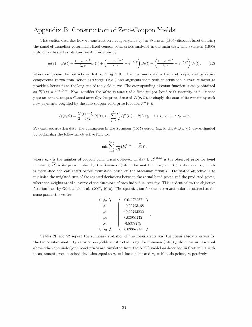
Appendix B: Construction of Zero-Coupon Yields

This section describes how we construct zero-coupon yields by the Svensson (1995) discount function using

the panel of Canadian government fixed-coupon bond prices analyzed in the main text. The Svensson (1995)

yield curve has a flexible functional form given by

yt(τ ) = β0(t) +1− e−λ1τ

λ1τβ1(t) +

(1− e−λ1τ

λ1τ− e−λ1τ

)β2(t) +

(1− e−λ2τ

λ2τ− e−λ2τ

)β3(t), (12)

where we impose the restrictions that λ1 > λ2 > 0. This function contains the level, slope, and curvature

components known from Nelson and Siegel (1987) and augments them with an additional curvature factor to

provide a better fit to the long end of the yield curve. The corresponding discount function is easily obtained

as P zct (τ ) = e−yt(τ)τ . Now, consider the value at time t of a fixed-coupon bond with maturity at t + τ that

pays an annual coupon C semi-annually. Its price, denoted Pt(τ, C), is simply the sum of its remaining cash

flow payments weighted by the zero-coupon bond price function P zct (τ ):

Pt(τ, C) =C

2

(t1 − t)

1/2P zct (t1) +

N∑

j=2

C

2P zct (tj) + P zc

t (τ ), t < t1 < . . . < tN = τ.

For each observation date, the parameters in the Svensson (1995) curve, (β0, β1, β2, β3, λ1, λ2), are estimated

by optimizing the following objective function

min

ny,t∑

i=1

1

Dit

(P data,it − P it )2,

where ny,t is the number of coupon bond prices observed on day t, P data,it is the observed price for bond

number i, P it is its price implied by the Svensson (1995) discount function, and Dit is its duration, which

is model-free and calculated before estimation based on the Macaulay formula. The stated objective is to

minimize the weighted sum of the squared deviations between the actual bond prices and the predicted prices,

where the weights are the inverse of the durations of each individual security. This is identical to the objective

function used by Gurkaynak et al. (2007, 2010). The optimization for each observation date is started at the

same parameter vector:

β0

β1

β2

β3

λ1

λ2

=

0.04173257

−0.02703468

−0.05262533

0.02954742

0.8378759

0.09652915

.

Tables 21 and 22 report the summary statistics of the mean errors and the mean absolute errors for

the ten constant-maturity zero-coupon yields constructed using the Svensson (1995) yield curve as described

above when the underlying bond prices are simulated from the AFNS model as described in Section 5.1 with

measurement error standard deviation equal to σε = 1 basis point and σε = 10 basis points, respectively.

37

Maturity Mean errors, σε = 1 basis pointin months Mean Std. dev. 5 percentile 1st quartile Median 3rd quartile 95 percentile

3 -4.09 2.83 -9.48 -5.70 -3.75 -2.16 0.096 -2.37 1.69 -5.78 -3.34 -1.99 -1.21 -0.1812 -0.32 0.42 -1.19 -0.61 -0.26 0.01 0.2024 0.78 0.60 -0.17 0.39 0.69 1.07 1.8236 0.43 0.47 -0.10 0.07 0.30 0.73 1.3260 -0.48 0.37 -1.11 -0.68 -0.45 -0.25 0.0584 -0.67 0.62 -1.94 -1.00 -0.51 -0.21 0.07120 -0.34 0.48 -1.06 -0.71 -0.27 0.05 0.31240 0.64 0.68 -0.36 0.07 0.57 1.02 1.91360 -1.32 1.14 -3.12 -2.23 -1.36 -0.49 0.41

Maturity Mean absolute errors, σε = 1 basis pointin months Mean Std. dev. 5 percentile 1st quartile Median 3rd quartile 95 percentile

3 6.79 2.55 4.00 4.80 6.15 7.84 11.576 3.89 1.63 2.19 2.64 3.42 4.65 6.9912 1.05 0.40 0.57 0.76 0.95 1.28 1.8324 1.42 0.51 0.87 1.03 1.27 1.64 2.3536 0.99 0.45 0.49 0.66 0.84 1.23 1.8460 1.05 0.25 0.74 0.87 1.01 1.14 1.4984 1.26 0.56 0.62 0.81 1.08 1.56 2.34120 0.94 0.28 0.61 0.73 0.86 1.11 1.43240 1.46 0.53 0.85 1.04 1.38 1.72 2.64360 3.09 0.81 1.93 2.40 2.97 3.62 4.62

Table 21: Summary Statistics of Errors of Constructed YieldsThe top panel reports the summary statistics of the mean errors between the true zero-coupon bond yields and

the zero-coupon bond yields constructed using the Svensson (1995) yield curve based on N = 100 simulated

data sets generated by the independent-factor AFNS model, each with a distribution of coupon bond prices

identical to the sample of Canadian fixed-coupon bond prices described in Section 2 and with each simulated

bond price being added an i.i.d. measurement error with zero mean and a uniform measurement error standard

deviation of σε = 1 basis point scaled by the bond’s duration. The bottom panel reports the corresponding

summary statistics of the mean absolute errors. All numbers are measured in basis points.

38

Maturity Mean errors, σε = 10 basis pointsin months Mean Std. dev. 5 percentile 1st quartile Median 3rd quartile 95 percentile

3 -3.00 2.59 -7.12 -4.61 -2.79 -1.02 1.446 -1.74 1.54 -4.37 -2.72 -1.66 -0.58 0.7112 -0.24 0.48 -1.07 -0.54 -0.30 0.06 0.6724 0.52 0.57 -0.52 0.22 0.46 0.85 1.4336 0.24 0.44 -0.37 -0.11 0.23 0.56 1.0460 -0.34 0.45 -1.16 -0.63 -0.26 -0.03 0.2584 -0.37 0.58 -1.56 -0.64 -0.28 0.06 0.34120 -0.14 0.43 -0.85 -0.52 -0.04 0.18 0.43240 0.27 0.65 -0.90 -0.18 0.31 0.61 1.19360 -0.90 1.31 -3.07 -1.78 -1.16 0.13 1.16

Maturity Mean absolute errors, σε = 10 basis pointsin months Mean Std. dev. 5 percentile 1st quartile Median 3rd quartile 95 percentile

3 12.48 1.44 10.47 11.50 12.21 13.15 15.586 7.84 0.91 6.67 7.24 7.62 8.33 9.3412 3.58 0.27 3.17 3.41 3.54 3.77 4.0524 3.52 0.26 3.09 3.36 3.52 3.69 3.9336 3.12 0.22 2.78 2.96 3.12 3.30 3.4660 3.13 0.22 2.80 2.97 3.14 3.28 3.5084 3.30 0.21 2.96 3.17 3.30 3.42 3.64120 2.88 0.21 2.48 2.75 2.85 3.00 3.19240 3.76 0.34 3.23 3.49 3.80 3.99 4.26360 9.34 1.28 7.58 8.48 9.12 10.13 11.53

Table 22: Summary Statistics of Errors of Constructed YieldsThe top panel reports the summary statistics of the mean errors between the true zero-coupon bond yields and

the zero-coupon bond yields constructed using the Svensson (1995) yield curve based on N = 100 simulated

data sets generated by the independent-factor AFNS model, each with a distribution of coupon bond prices

identical to the sample of Canadian fixed-coupon bond prices described in Section 2 and with each simulated

bond price being added an i.i.d. measurement error with zero mean and a uniform measurement error standard

deviation of σε = 10 basis points scaled by the bond’s duration. The bottom panel reports the corresponding

summary statistics of the mean absolute errors. All numbers are measured in basis points.

39

Appendix C: The Extended Kalman Filter Estimation

This appendix describes the model estimations based on the Kalman filter and the extended Kalman filter.

For affine Gaussian models in general, the conditional mean vector and the conditional covariance matrix are26

EP [Xt+∆t|Ft] = (I − exp(−KP∆t))θP + exp(−KP∆t)Xt,

V P [Xt+∆t|Ft] =

∫ t+∆t

t

e−KP sΣΣ′−(KP )′sds,

where ∆t is the time between observations. Conditional moments of discrete observations are computed and

the state transition equation is obtained as

Xt = (I − exp(−KP∆t))θP + exp(−KP∆t)Xt−∆t + ξt,

where ξt refers to the Gaussian state innovations.

In the standard Kalman filter, the measurement equation is linear

yt = A+BXt + εt,

and the assumed error structure is

(ξt

εt

)∼ N

[(0

0

),

(Q 0

0 H

)],

where the matrix H is assumed to be diagonal, while the matrix Q has the following structure

Q =

∫ ∆t

0

e−KP sΣΣ′−(KP )′sds.

In addition, the transition and measurement errors are assumed to be orthogonal to the initial states. Due to

the assumed stationarity, the Kalman filter is initialized at the unconditional mean and variance of the state

variables under the P -measure, i.e., X0 = θP and Σ0 =∫∞

0e−K

P sΣΣ′−(KP )′sds. Denote the information

available at time t by Yt = (y1, y2, . . . , yt), and denote model parameters by ψ. Let ∆t = 1 and consider period

t− 1 and suppose that the state update Xt−1 and its mean square error matrix Σt−1 have been obtained. The

prediction step is

Xt|t−1 = EP [Xt|Yt−1] = ΦX,0t (ψ) + ΦX,1t (ψ)Xt−1,

Σt|t−1 = ΦX,1t (ψ)Σt−1ΦX,1t (ψ)′ +Qt(ψ),

where ΦX,0t = (I − exp(−KP∆t))θP , ΦX,1t = exp(−KP∆t), and Qt =∫∆t

0e−K

P sΣΣ′−(KP )′sds.

In the time-t update step, Xt|t−1 is improved by using the additional information contained in Yt, i.e.,

Xt = E[Xt|Yt] = Xt|t−1 + Σt|t−1B(ψ)′F−1t vt,

Σt = Σt|t−1 − Σt|t−1B(ψ)′F−1t B(ψ)Σt|t−1,

where

vt = yt −E[yt|Yt−1] = yt − A(ψ)−B(ψ)Xt|t−1,

Ft = cov(vt) = B(ψ)Σt|t−1B(ψ)′ +H(ψ),

H(ψ) = diag(σ2ε(τ1), . . . , σ

2ε(τN)).

26Throughout, conditional and unconditional covariance matrices are calculated using the analytical solutionsprovided in Fisher and Gilles (1996).

40

At this point, the Kalman filter has delivered all ingredients needed to evaluate the Gaussian log likelihood,

which reads

LEKF (ψ) ≡ log l(y1, . . . , yT ;ψ) =T∑

t=1

(− N

2log(2π)− 1

2log |Ft| − 1

2v′tF

−1t vt

),

where N is the number of observed yields. Now, the likelihood is numerically maximized with respect to

ψ using the Nelder-Mead simplex algorithm. Upon convergence, the standard errors are obtained from the

estimated covariance matrix,

Ω(ψ) =1

T

[ 1T

T∑

t=1

∂ log lt(ψ)

∂ψ

∂ log lt(ψ)

∂ψ

′]−1

,

where ψ denotes the estimated model parameters.

In model estimations with coupon bond prices in the one-step approach and for the B-AFNS model using

the two-step approach, the extended Kalman filter is needed because the measurement equations are no longer

affine functions of the states. Instead, the measurement equation takes the general form

Pi

t(ti0, τ

i)

Dit(t

i0, τ

i)= g(Xt; t

i0, τ

i, ψ) + εit.

In the extended Kalman filter, this equation is linearized using a first-order Taylor expansion around the best

guess of Xt in the prediction step of the Kalman filter algorithm. Thus, in the notation introduced above, this

best guess is denoted Xt|t−1 and the approximation is given by

g(Xt; ti0, τ

i, ψ) ≈ g(Xt|t−1; ti0, τ

i, ψ) +∂g(Xt; t

i0, τ

i, ψ)

∂Xt

∣∣∣Xt=Xt|t−1

(Xt −Xt|t−1).

Thus, by defining

At(ψ) ≡ g(Xt|t−1; ti0, τ

i, ψ)− ∂g(Xt; ti0, τ

i, ψ)

∂Xt


Xt|t−1 and Bt(ψ) ≡ ∂g(Xt; ti0, τ

i, ψ)

∂Xt


,

the measurement equation can be given on an affine form as

Pi

t(ti0, τ

i)

Dit(t

i0, τ

i)= At(ψ) +Bt(ψ)Xt + εit,

and the steps in the algorithm proceed as previously described, except that the standard errors are obtained

from

ΩQML(ψ)=

1

TH(ψ)−1

[1

T

T∑

t=1

∂ log lt(ψ)

∂ψ

∂ log lt(ψ)

∂ψ

′]H(ψ)−1,

where H(ψ).is the Hessian matrix evaluated as described in Harvey (1989).

41

Appendix D: The One-Step Approach and Full ML Estimation

To describe the procedure for concentrating out X1:T of the log-likelihood function in equation (10),

observe that

∂L(ψ|Y1:T

)

∂Xt= −dtR−1

w (Xt − h (Xt−1;ψ)) (13)

+hX (Xt;ψ)′R−1

w (Xt+1 − h (Xt;ψ))

−gX (Xt;ψ)′R−1

ε,t (Yt − g (Xt;ψ))

= 0

for t = 1, 2, ..., T , where d1 = 0 and dt = 1 for t > 1. The matrix hX (Xt;ψ) ≡ ∂h(Xt;ψ)∂X′

tand denotes the nx×nx

Jacobian of h (Xt;ψ) with respect to Xt, and similarly, gX (Xt;ψ) ≡ ∂g(Xt;ψ)∂X′

twith dimensions ny,t × nx. Let

X(i)1:T denote the points around which the system in (8) and (9) is linearized. That is,

Yt = g(X

(i)t ;ψ

)+ gX

(X

(i)t ;ψ

)(Xt −X

(i)t

)+ εt, (14)

Xt+1 = h(X

(i)t ;ψ

)+ hX

(X

(i)t ;ψ

)(Xt −X

(i)t

)+ wt+1. (15)

For a given value of ψ, let X1:T (ψ) denote the state estimates from running the Kalman smoother on the

linearized system in equations (14) and (15). As shown in Durbin and Koopman (2001), X1:T (ψ) then solves

the following system of equations

−dtR−1w

(Xt − h

(X

(i)t−1;ψ

)− hX

(X

(i)t−1;ψ

)(Xt−1 (ψ)−X

(i)t−1

))(16)

+hX(X

(i)t ;ψ

)′R−1w

(Xt+1 − h

(X

(i)t ;ψ

)− hX

(X

(i)t ;ψ

)(Xt (ψ)−X

(i)t

))

−gX(X

(i)t ;ψ

)′R−1ε,t

(Yt − g

(X

(i)t ;ψ

)− gX

(X

(i)t ;ψ

)(Xt (ψ)−X

(i)t

))

= 0

for t = 1, 2, ..., T . Accordingly, when Xt (ψ) = X(i)t (ψ) for all t, the conditions in equations (16) reduces to

those in equations (13), meaning that X1:T (ψ) is the ML estimates of the states for a given value of ψ. The

iterative procedure to find this solution is as follows:

Step 1 Run the Extended Kalman filter and smoother on the system in equations (8) and (9) to obtain

XEKF1:T (ψ). Set i = 1 and let X

(i)1:T (ψ) = XEKF

1:T (ψ).

Step 2 Run the Extended Kalman filter and smoother on the linearized system in equations (14) and (15) to

obtain X1:T (ψ).

Step 3 If∣∣∣Xt (ψ)−X

(i)t (ψ)

∣∣∣ > ǫ for any t, where ǫ is a small number, let i = i+ 1 and X(i)1:T (ψ) = X1:T (ψ)

and go to step 2, otherwise stop.

Let X1:T (ψ) denote the states from this procedure, which depends on ψ. The concentrated log-likelihood

function is then Lc (ψ|Y1:T ) ≡ L(ψ, X1:T (ψ) |Y1:T

), which we optimize across ψ to obtain the ML estimates.

The asymptotic standard errors for ψML are obtained in a standard fashion, i.e.,

AV ar(ψML

)=

[T∑

t=1

sci

(ψML

)sci

(ψML

)′]−1

, (17)

where the concentrated score sci

(ψML

)is computed by numerical differentiation of Lc (ψ|Y1:T ).

42

Appendix E: Full ML Estimation with Stochastic Volatility

Suppose Xt evolves as

Xt+1 = h (Xt; θ) + f (Xt, εt+1; θ) , (18)

where the f -function accommodates stochastic volatility in the dynamics of Xt. Lagging equation (18) by one

period and inserting it into equation (8) gives

Yt = g (h (Xt−1; θ) + f (Xt−1, εt) ; θ)︸︷︷︸g(Xt−1,εt;θ)

+ vt (19)

[Xt

εt+1

]=

[h (Xt−1; θ) + f (Xt−1, εt)

0

]+

[0

ut+1

]

where ut+1 ∼ NID (0, Rε). Thus, by expanding the state vector to Xt =[X ′t−1 ε′t

]′, the law of motion

in equation (18) with nonlinearities between the states and the innovations can be rewritten into an extended

system with only linear innovations as in equations (8) and (9).

43

Appendix F: Formulas for Short Rate Expectations and TermPremiums

In this appendix, we derive the analytical formulas for short-rate expectations and term premiums in the

independent-factor AFNS model. Recall that term premium is defined as

TPt(τ ) = yt(τ )− 1

τ

∫ t+τ

t

EPt [rs]ds.

Furthermore, recall that for affine stochastic differential equations of the form

dXt = KP (θP −Xt)dt+ ΣdWPt ,

the conditional expectation is given by

EPt [Xt+τ ] = (I − exp(−KP τ ))θP + exp(−KP τ )Xt.

In the AFNS model, the instantaneous short rate is defined as

rt = Lt + St,

while the specification of the P -dynamics considered is given by

dLt

dSt

dCt

=

κP11 0 0

0 κP22 0

0 0 κP33

θP1

θP2

θP3

−

Lt

St

Ct

dt+

σ11 0 0

0 σ22 0

0 0 σ33

dWL,Pt

dW S,Pt

dWC,Pt

.

Thus, the mean-reversion matrix is given by

KP =

κP11 0 0

0 κP22 0

0 0 κP33

.

Its matrix exponential can be calculated analytically and is given by

exp(−KP τ ) =

e−κP11τ 0 0

0 e−κP22τ 0

0 0 e−κP33τ

.

Now, the conditional mean of the state variables is

EPt [Xt+τ ] = θP +

e−κP11τ 0 0

0 e−κP22τ 0

0 0 e−κP33τ

Lt − θP1

St − θP2

Ct − θP3

=

θP1 + e−κP11τ (Lt − θP1 )

θP2 + e−κP22τ (St − θP2 )

θP3 + e−κP33τ (Ct − θP3 )

.

In order to get back to the term premium formula, we note that the conditional expectation of the instantaneous

short rate process is:

EPt [rs] = EPt [Ls + Ss]

= θP1 + e−κP11

(s−t)(Lt − θP1 ) + θP2 + e−κP22

(s−t)(St − θP2 ).

Next, we integrate the expected short rate over the time interval from t to t+ τ as in the definition of the term

44

premium:

∫ t+τ

t

EPt [rs]ds =

∫ t+τ

t

(θP1 + e−κ

P11

(s−t)(Lt − θP1 ) + θP2 + e−κP22

(s−t)(St − θP2 ))ds

= (θP1 + θP2 )τ + (Lt − θP1 )1− e−κ

P11τ

κP11+ (St − θP2 )

1− e−κP22τ

κP22.

The relevant term to go into the term premium formula is the average expected short rate

1

τ

∫ t+τ

t

EPt [rs]ds = θP1 + θP2 + (Lt − θP1 )1− e−κ

P11τ

κP11τ+ (St − θP2 )

1− e−κP22τ

κP22τ.

The final expression for the term premium is then given by

TPt(τ ) = yt(τ )− 1

τ

∫ t+τ

t

EPt [rs]ds

= Lt +1− e−λτ

λτSt +

(1− e−λτ

λτ− e−λτ

)Ct − A(τ )

τ

−θP1 − θP2 − (Lt − θP1 )1− e−κ

P11τ

κP11τ− (St − θP2 )

1− e−κP22τ

κP22τ

=(1− 1− e−κ

P11τ

κP11τ

)Lt +

(1− e−λτ

λτ− 1− e−κ

P22τ

κP22τ

)St +

(1− e−λτ

λτ− e−λτ

)Ct

−(1− 1− e−κ

P11τ

κP11τ

)θP1 −

(1− 1− e−κ

P22τ

κP22τ

)θP2 − A(τ )

τ.

45

References

Andersen, Torben G., Nicola Fusari, and Viktor Todorov, 2015, “Parameter Inference and

Dynamic State Recovery from Option Panels,” Econometrica, Vol 83, No. 3, 1081-1145.

Andreasen, Martin M., 2013, “Non-Linear DSGEModels and The Central Difference Kalman

Filter,” Journal of Applied Econometrics, Vol. 28, 929-955.

Andreasen, Martin M. and Bent Jesper Christensen, 2015, “The SR Approach: A New Esti-

mation Procedure for Non-Linear and Non-Gaussian Dynamic Term Structure Models,”

Journal of Econometrics, Vol. 184, No. 2, 420-451.

Andreasen, Martin M., Jens H. E. Christensen, and Simon Riddell, 2017, “The TIPS Liq-

uidity Premium,” Working Paper 2017-11, Federal Reserve Bank of San Francisco.

Bai, Jushan, 2003, “Inferential Theory for Factor Models of Large Dimensions,” Economet-

rica, Vol. 71, No. 1, 135–171.

Bai, Jushan, and Serena Ng, 2002, “Determining the Number of Factors in Approximate

Factor Models,”Econometrica, Vol. 70, No. 1, 191–221.

Bauer, Michael D., Glenn D. Rudebusch, and Jing (Cynthia) Wu, 2012, “Correcting Esti-

mation Bias in Dynamic Term Structure Models,” Journal of Business and Economic

Statistics, Vol. 30, No. 3, 454-467.

Bjork, Tomas and Bent J. Christensen, 1999, “Interest Rate Dynamics and Consistent For-

ward Rate Curves,” Mathematical Finance, Vol. 9, 323-348.

Black, Fisher, 1995, “Interest Rates as Options,” Journal of Finance, Vol. 50, No. 7,

1371-1376.

Bliss, Robert R., 1996, “Testing Term Structure Estimation Methods,” Advances in Futures

and Options Research, Vol. 9, 197-231.

Bolder, David J., Grahame Johnson, and Adam Metzler, 2004, “An Empirical Analysis of

the Canadian Term Structure of Zero-Coupon Interest Rates,” Bank of Canada Working

Paper No. 2004-48.

Bollerslev, Tim and Jeffrey M. Wooldridge, 1992, “Quasi-Maximum Likelihood Estimation

and Inference in Dynamic Models with Time-Varying Covariances,” Econometrics Re-

views, Vol. 11, No. 2, 143-172.

Campbell, John Y. and Robert J. Shiller, 1991, “Yield Spread and Interest Rate Movements:

A Bird’s Eye View,” Review of Economic Studies, Vol. 58, No. 3 , 495-514.

46

Christensen, Jens H. E., Francis X. Diebold, and Glenn D. Rudebusch, 2009, “An Arbitrage-

Free Generalized Nelson-Siegel Term Structure Model,” Econometrics Journal, Vol. 12,

No. 3, C33-C64.

Christensen, Jens H. E., Francis X. Diebold, and Glenn D. Rudebusch, 2011, “The Affine

Arbitrage-Free Class of Nelson-Siegel Term Structure Models,” Journal of Econometrics,

Vol. 164, No. 1, 4-20.

Christensen, Jens H. E. and Glenn D. Rudebusch, 2015, “Estimating Shadow-Rate Term

Structure Models with Near-Zero Yields,” Journal of Financial Econometrics, Vol. 13,

No. 2, 226-259.

Christensen, Jens H. E. and Glenn D. Rudebusch, 2016, “Modeling Yields at the Zero Lower

Bound: Are Shadow Rates the Solution?,” in Eric Hillebrand, Siem Jan Koopman

(ed.) Dynamic Factor Models (Advances in Econometrics, Volume 35) Emerald Group

Publishing Limited, 75-125.

Dai, Qiang and Kenneth J. Singleton, 2000, “Specification Analysis of Affine Term Structure

Models,” Journal of Finance, Vol. 55, No. 5, 1943-1978.

Dai, Qiang, Kenneth J. Singleton, and Wei Yang, 2004, “Predictability of Bond Risk Premia

and Affine Term Structure Models,” Manuscript, Graduate School of Business, Stanford

University.

Driessen, Joost, 2005, “Is Default Event Risk Priced in Corporate Bonds?,” Review of Fi-

nancial Studies, Vol. 18, No. 1, 165-195.

Duffee, Gregory R., 1999, “Estimating the Price of Default Risk,” Review of Financial

Studies, Vol. 12, No. 1, 197-226.

Duffee, Gregory R., 2002, “Term Premia and Interest Rate Forecasts in Affine Models,”

Journal of Finance, Vol. 57, No. 1, 405-443.

Durbin, J. and S. J. Koopman, 2001, “Time Series Analysis by State Space Methods,”

Oxford University Press, Oxford.

Fama, Eugene F., 1976, “Forward Rates as Predictors of Future Spot Rates,” Journal of

Financial Economics, Vol. 3, No. 4, 361-377.

Faria, Adriano and Caio Almeida, 2017, “A Hybrid Spline-Based Parametric Model for the

Real Yield Curve,” Manuscript, FGV Rio de Janeiro.

Filipovic, Damir and Sander Willems, 2016, “Exact Smooth Term Structure Estimation,”

Manuscript, EPFL and Swiss Finance Institute.

47

Fisher, Mark and Christian Gilles, 1996, “Term Premia in Exponential-Affine Models of the

Term Structure,” Manuscript, Board of Governors of the Federal Reserve System.

Fontaine, Jean-Sebastien and Rene Garcia, 2012, “Bond Liquidity Premia,” Review of Fi-

nancial Studies, Vol. 25, No. 4, 1207-1254.

Gurkaynak, Refet S., Brian Sack, and Jonathan H. Wright, 2007, “The U.S. Treasury Yield

Curve: 1961 to the Present,” Journal of Monetary Economics, Vol. 54, No. 8, 2291-

2304.

Gurkaynak, Refet S., Brian Sack, and Jonathan H. Wright, 2010, “The TIPS Yield Curve

and Inflation Compensation,” American Economic Journal: Macroeconomics, Vol. 2,

No. 1, 70-92.

Hahn, Jinyong and Whitney Newey, 2004, “Jackknife and Analytical Bias Reduction for

Nonlinear Panel Models,” Econometrica, Vol. 72, No. 4, 1295-1319.

Harvey, A.C., 1989, Forecasting, structural time series models and the Kalman filter, Cam-

bridge: Cambridge University Press.

Kim, Don H. and Kenneth J. Singleton, 2012, “Term Structure Models and the Zero Bound:

An Empirical Investigation of Japanese Yields,” Journal of Econometrics, Vol. 170, No.

1, 32-49.

Krippner, Leo, 2013, “A Tractable Framework for Zero Lower Bound Gaussian Term Struc-

ture Models,” Discussion Paper 2013-02, Reserve Bank of New Zealand.

Nelson, Charles R. and Andrew F. Siegel, 1987, “Parsimonious Modeling of Yield Curves,”

Journal of Business, Vol. 60, No. 4, 473-489.

Pancost, N. Aaron, 2017, “Zero-Coupon Yields and the Cross-Section of Bond Prices,”

Chicago University, Working Paper, 1-66.

Steeley, James M., 2008, “Testing Term Structure Estimation Methods: Evidence from the

UK STRIPs Market,” Journal of Money, Credit and Banking, Vol. 40, No. 7, 1489-1512.

Svensson, Lars E. O., 1995, “Estimating Forward Interest Rates with the Extended Nelson-

Siegel Method,” Quarterly Review, No. 3, Sveriges Riksbank, 13-26.

Swanson, Eric T. and John C. Williams, 2014, “Measuring the Effect of the Zero Lower

Bound on Medium- and Longer-Term Interest Rates,” American Economic Review,

Vol. 104, No. 10, 3154-3185.

48

term structure analysis with big data - frbsf.org · pdf fileour benchmark dtsm is the...

Documents