tenure and forest management in india: impacts on … and forest management ... documented cases of...

1

Tenure and forest management in India: Impacts on

equity and efficiency of Van Panchayats in Uttarakhand,

India

Abstract

In policy circles and well as the academia, the success of communal control of forest resources is

mostly defined in terms of the conservation objectives rather than distributional fairness. In this

paper we evaluate community management of forest in terms of its distributional outcomes,

using the example of Van Panchayats in Uttrakhand (India). We test how caste and asset-holding

affect resource extraction in villages with and without community forestry. We find that while

Van Panchayats lead to reduced firewood collection for every economic group, the reduction is

significantly higher among asset poor households. However we don’t find such adversely

proportional reduction on grounds of caste.

The paper also studies the impact of communal control on the efficiency of firewood

production. We find that restrictions on collection in a Van Panchayat regime ensure a

downward shift in the average product (of labour spent on firewood collection) schedule.

However they also induce a reduction in the time spent on firewood collection. We do not

observe increased efficiency due to regeneration of forests under communal control.

2

1. Introduction

Environmentalists and conservationists have often advocated communal control of

natural resources as a way to ensure its judicious and sustainable use (Colchester 1994, Kothari

2011). Since the early 1980s, economists, sociologists and cultural anthropologists have

documented cases of sustainable natural resource management by local communities (Acheson

1988; Ostrom 1990; Berkes 1986). This was followed by sophisticated theoretical models (often,

if not always, based on co-operative game theory) that showed that “Commons” –resources that

are jointly managed, often follow trajectories that are not “tragic” (Sethi and Somanathan 1996;

Chichilnisky 1994). Once Ostrom and others had demolished the infallibility of the “Tragedy of

the Commons”, policy makers around the world started viewing communal control as a panacea

to solve all kinds of natural resource problems.

South Asia also followed the trend by adopting policies promoting communal or joint

management of natural resources. The forestry sector saw major action in terms of transfer of

managerial authority, and in some cases even ownership, to local communities. In India, this

took the form of joint forest management (JFM) in the early nineties. JFM involves local

communities in conservation of forest with the promise of pecuniary and non-pecuniary benefits

on successful completion of such efforts. However, JFM was viewed with skepticism by

proponents of community forestry as the state still played a substantial role in forest management

(Sarin et al. 2003). The failure of JFM in achieving its objectives (Lele and Borgoyary 2008;

Banerjee 19971) was contrasted sharply with the success stories of true community management

in the form of Van Panchayats in Uttrakhand and informal community forest management in

Orissa (Somanathan et al. 2005; Baland et al. 2010; Singh et al. 2005).

However, in most of these studies success was defined in terms of the ability of these

management regimes in achieving their conservation objectives. While only a few of the studies

measured forest quality directly (for exceptions, see Somanathan et al. 2005, Baland et al. 2010),

others studied the impact of decentralization on forest resource collection with the implicit

assumption that reduced resource collection improved forest quality (Edmonds 2002;

Bandhyopadhyay and Shyamsunder 2004).

The issue of intra-community distributional fairness was rarely the criteria to measure

success. In highly unequal and stratified societies of South Asia, it is important to measure the

success of a policy in terms of its distributional effects. In this chapter we try to evaluate

community management of forest in terms of its intra-community distributional outcomes.

Related to the question of intra-community equity is the question of economic efficiency of a

1Banerjee writes “… although the potential of JFM is high, in the overall Indian forestry situation, the impact is

small. Only 2% of the forests of India have been covered by JFM so far. Only degraded forests are being offered for

joint forest management. Leaving out the closed and high forests from the JFM operation is counterproductive as

the degraded forests of to-day are the closed forests of yesteryear. And the fate of the present day closed forests will

be the same over time unless the people are involved in their management.” (Page 16)

3

natural resource management regime. Economic efficiency is a metric that is distinctly different

from the conservation metrics usually used to judge community management regimes. Given the

focus on conservation objectives, most analyses emphasize the role of institutions in reducing

resource extraction. The question of efficient economic management is usually ignored. It should

be noted that the metrics of conservation and economic efficiency are often not directly related.

A forest from which no resource is extracted and on which no scientific silvicultural

management is practiced can have high canopy cover and basal volume. However, given its low-

intensive management (primarily protection) such a forest is unable to achieve its economic

potential and is hence inefficient. In this chapter, we focus on two issues of interest: The first is

the implications of assets and caste on access to firewood in villages with differences in forest

management. The second aspect is how local forest management affects the efficiency in

collection. More specifically, we test if the marginal productivity of firewood collection with

respect to labour is systematically higher in locally managed forests as compared to forests under

state control. We do this by using the specific example of Van Panchayats in Uttrakhand, India.

2. Hypotheses with respect to equity and efficiency implications of local forest

management

There might be several reasons for a change in distributional outcome due to a change in

resource regime. It has been widely documented that the history of state control of forests is also

a history of widespread forest degradation. It is suggested that heavy deforestation occurs during

nationalization as people feel that their forests are being taken away from them (Gilmour et al.

1989;Guha 1989;Tamuli and Choudhury 2009). Since the government does not have the ability

to monitor and control collection, forests are in effect converted to open access resources. It

might be the case that as free entry ensures zero rents, the village elite have no incentive to

monitor and control collection. Analogously, restrictions on entry imposed by communitarian

regimes create possibilities for rent and hence create an environment where the community elite

has an incentive to restrict forest use by the marginalized within the community.

In this spirit, Bardhan (2010) argues that the ease of forming collusions and the absence

of scrutiny by media and civil society can lead to adverse distributional outcomes from

devolution of managerial power. He also observes that when the elite cannot capture access to

public goods, there might be a danger of them seceding from the system. In the absence of active

support from the elite, the structure might collapse. The non-elite can foresee this sequence of

events and hence might accept elite capture to sustain local institutions. Such arguments motivate

analyses of implications on social groups, e.g. caste, in addition to the use of income group as

distributional criterion.

Studies on the impact of a resource control regime on the intra-community distribution of

resource collected are not very common. Most studies on this issue look at inequities across

income levels, often neglecting inequities across social groups. Studying equity issues in

4

community forestry in the middle hills of Nepal2, Adhikari (2008) observes “Local elites are

found to be advantaged in both accessing the decision making committee and extracting benefits

from the forest”. Sociologists writing on community control programs in India have often

observed that such programs benefit the rural elite at the cost of the marginalized: poor, women

and Dalits. Omvedt (1997) documents how Hadis (an untouchable caste) were not allowed to

fish in the Chilka Lake (Orissa) when fishing in the area was communally organized.

Sundar (2000) argues that community forestry schemes, such as JFM in India, adversely

affect the poor by closing access to nearby forests. The rich, who have access to alternate sources

of fuelwood and can afford non-biomass fuels, are not affected. Sarin et al. (1998) and Kumar

(2002) support the view of Sundar (2000). Agarwal (2001) studies issues of gender equity and

observes that women, who have no role in the decision making process of JFM, is the group that

is most adversely affected by JFMs. Agarwal (2007) shows that women, who are the household

members with the main responsibility of firewood collection, often have to bear a large share of

the costs associated with community forestry. In their recent work on JFM in Andhra Pradesh,

Saito-Jensen and Jensen (2010) show that “geographical boundaries created through JFM policy,

interact with existing social boundaries of caste and gender to ensure an asymmetric distribution

of costs and benefits from JFM”. In Nepal, studies have shown that many of the forest user

groups suffer from elite capture. Low castes and the poor are often excluded from the decision

making process, which ensure that funds are often invested in projects that are advantageous for

the rich (Banjade et al. 2004; Malla et al. 2003; Timsina 2003).

Although these studies highlight the existing inequities under communal management of

resources, they don't study how such systems perform in terms of equity compared to other

modes of resource control like centralized state control, or private ownership. Given the

predominant orientation of the literature, the hypotheses to be tested in this study with regards to

equity are that asset poor and low caste households are made worse off with respect to firewood

collection under Van Panchayat management compared to government management.

The literature on economic efficiency of alternative forest regimes is even leaner. Sakurai

et. al. (2004) compares ‘the management performance of timber production among three

management regimes in Nepal: private forestry, community forestry with collective management

and community forestry with centralized management’. They find that centralized management

2 Nepal has a lot of similarity with Uttarakhand in terms of its geography. Both the regions have parts that overlap

the Greater Himalayas, the Middle Himalayas, Shivaliks and the Terai. They share demographic similarity as well

with more than 80% of the population being Hindus. However, Uttarakhand has a higher percentage of

"Untouchable" castes (Dalits) (around 17%) compared to Nepal (12%). Nepal, on the other hand, has a higher

percentage of tribals or Janajatis. While informal communal forestry institutions are old in both Uttarakhand and

Nepal, formal institutions evolved in Uttrakhand much earlier than Nepal. Van Panchayats were set up by the

British-Indian government in the 1930s as a response to protest movements by people who felt threatened by the

colonial forestry policy. The community forestry program in Nepal was initiated by the government in late 1970s in

response to high rates of deforestation due to nationalization of forests. Unlike JFM committees in India, both Van

Panchayats in Uttarakhand and FUGs in Nepal enjoy substantial autonomy in decision making.

5

leads to higher revenue and profit from timber production when compared to community

management. In fact, Sakurai et al (2004) identifies a negative trade-off between conservation

objective and economic efficiency: “while collective management is more efficient for protection

of trees due to mutual supervision, profit seeking private management or centralized

management is more efficient than collective management for silvicultural operations due to

superior work incentives”. Chand (2011) also shows that production is not organized efficiently

in community forests of Nepal. Köhlin and Amacher (2005) estimate firewood production

functions for different firewood sources and different categories of labour to calculate the

marginal productivity of labour for each of these categories. The comparison between collection

in plantations under local management (‘social forests’) and natural forests (government

controlled but de facto open access) reveal that the marginal productivity of men from villages

with natural forests only, are systematically lower than the marginal productivity of men from

villages with social forests. While men seem to be able to equate the marginal productivity

between different sources of fuel, women had significantly higher productivity in their collection

in the nearby managed plantations. Caste was also a significant factor in explaining collection

behavior. Köhlin and Amacher (2005) found two efficiency gains from the social forestry

intervention – a direct improvement through the increased access to fuel in the plantations and

also an indirect effect through increased productivity in collection from the subsequently less

degraded natural forests.

Our hypothesis with regards to efficiency is that the long-term protection of Van

Panchayat forests, with its demonstrated positive effects on forest quality (Baland et al. 2010),

has been at the expense of forest collection.

3. Van Panchayats in Uttarakhand

Since the Van Panchayats in Uttarakhand are geographically distinct and have historic

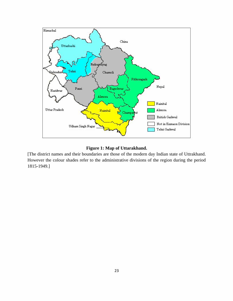
roots, we need to explain their background. The state of Uttarakhand is divided into two parts: (i)

Garhwal, consisting of the districts of Chamoli, Dehradun, Haridwar, PauriGarhwal,

Rudraprayag, TehriGarhwal, and Uttarkashi and (ii) Kumaon, consisting of the districts of

Udham Singh Nagar, Nainital, Champawat, Almora, Bageshwar and Pithoragarh. Prior to India’s

independence in 1947, the British rule extended to all these districts except Uttarkashi and

TehriGarhwal. These two districts constituted the princely state of TehriGarhwal3.

[Figure 1: District Map of Uttarakhand.]

3Champawat, Almora, Bageshwar and Pithoragarh constituted the erstwhile British district of Almora (Kumaon Division).

Nainital and Udham Singh Nagar were a part of the British district of Nainital (Kumaon Division). Chamoli, Rudraprayag and

Pauri constituted the British Garhwal District (Kumaon District). Haridwar and Dehradun were neither a part of the princely state

of TehriGarhwal nor a part of the Kumaon Division of United provinces.

http://en.wikipedia.org/wiki/Chamoli_District

http://en.wikipedia.org/wiki/Dehradun_District

http://en.wikipedia.org/wiki/Haridwar_District

http://en.wikipedia.org/wiki/Pauri_Garhwal

http://en.wikipedia.org/wiki/Rudraprayag_District

http://en.wikipedia.org/wiki/Tehri_Garhwal_District

http://en.wikipedia.org/wiki/Uttarkashi_District

6

The Van Panchayats in Uttarakhand owe their origins to the British Colonial Forest

policy. After the British took control over Kumaon and British Garhwal, between 1840 and

1910, they brought most forest areas of the Kumaon division under their control to exploit forest

resources commercially. The introduction of railways in India and the process of rapid capitalist

industrialization in Britain had generated a huge demand for Indian timber. This demand

pressure forced the British Colonial Government to establish the sole authority of the colonial

state on forest resources. In 1910-17, the British government tightened its control over forest

resources by notifying 7,500 square kilometers of commons as reserve forests, thus restricting

people’s access to forest produce. Increased presence of the forest department also led to an

increase in ‘collie utar’ (forced labour) and ‘bardaish’ (forced supply of provisions from villagers

to colonial bureaucrats). Popular resistance in the form of rebellions and incendiarism made the

state pass the "Van Panchayat Act" in 1931, according to which 30% of the forests (Class I

Forests and Civil Forests) were given back to the villagers, to be controlled and managed by the

relatively autonomous panchayats. However, to get Van Panchayat status the ‘gram sabha’

(village assembly) had to apply to the divisional commissioner. The application had to be signed

by at least 66% of the adult population of the village4. The managing committee of the Van

Panchayat (5 to 13 members) was informally elected by the villagers by a show of hands. Today,

more than 6000 Van Panchayats control the use of 13.63% of the forest areas in Uttarakhand.

While all Van Panchayats in the state are governed by the same government law, the

Forest Panchayat Act, at village level, rules and regulations may differ. Day-to-day management

of the panchayat forests is governed by the rules the Van Panchayat creates in regular meetings.

Mukherjee (2003) mentions four identifiable working rules in limiting use, monitoring and

sanctioning violations and arbitration. Agarwal (1999) lists the functions of Van Panchayats as

follows: a) Prevent indiscriminate felling and tempering of fencing by villagers. b) Ensure

equitable distribution of forest produce amongst members. c) Earmark eligible trees for felling.

d) Prevent encroachment of forest land by villagers for agricultural and other purposes. e) Fix

boundary pliers and ensure proper maintenance of pillars. f) Carry out forestry operations as per

advice of forest experts from forest department.

In the process of discharging these functions, Van Panchayat committees are allowed to

impose fines, seize and impound cattle and forfeit weapons of violators/offenders. In addition to

such formal measures, informal social sanctions can also be used. The Van Panchayats have the

ability to raise revenues by selling grass, fallen twigs, stones and slates to local markets, tapping

resins and felling trees with prior approval of the forest department and auctioning mature trees.

Thus, the nature of Van Panchayat rules is such that it is conceivable that they can be

used to protect the interests of the elite. The fact that application can be made by 20% of the

population and that elections to the managing committee are not done formally through secret

4The ‘Panchyati Van Nimyamavali, 1993’ (Van Panchayati Rules of 1993) reduced the number to 20% (Agarwal 1999).

7

ballot, can conceivably lead to a capture of such institutions by the powerful village elite, who in

turn enacts rules that go against the interests of the marginalized. For example, Agarwal (1999)

notes “In Uttarakhand, women are responsible to carry fuelwood and fodder from forests, and

they know forests more than men, still their participation in Van Panchayats and its decision

making process is negligible. As a result, fodder and fuelwood yielding species are neglected and

commercial ones encouraged”.

4. Data:

In this paper, we use data collected by the Planning and Policy Research Institute of the

Indian Statistical Institute, New Delhi.5 The objective of this survey was to study “a large

number of villages within a fairly common agro-climatic region with similar ecological

characteristics but with disparate socio-economic structure, market access and governance

patterns with enough independent variation in each of these factors”. Household surveys were

done in 165 villages over a period of three years. The survey restricted its focus to villages at an

average altitude of 1800 metres to 3000 metres. The sampling frame was adjusted accordingly.

On the basis of census data, villages with less than 20 households were dropped and the

remaining set of villages were stratified on the basis of altitude, number of households in a

village and distance to the nearest town. Villages were selected randomly from each stratum.

The entire exercise was conducted separately for Himachal Pradesh and Uttarakhand and

the final sample consisted of 82 villages in Himachal Pradesh and 83 villages in Uttarakhand. In

this paper we only use the data from Uttarakhand since Van Panchayats are only found in this

state. The sample villages for Uttarakhand are from the 6 districts of Uttarkashi, Chamoli,

Nainital, Bageshwar, Champawat and Pithoragarh.

A sample of 20 households was surveyed in each village. The households were selected

on the basis of a stratification procedure where the strata were formed by combining the

landholding and caste-distribution in the village. Three questionnaires were used to conduct

surveys in each village: (i) a household questionnaire that dealt with the socio-economic

structure of the household and its dependence on forests, (ii) a village questionnaire that was

designed to secure information on a number of village level characteristics such as

demographics, access to physical and social infrastructure and the market environment and (iii)

an ecology questionnaire that was framed essentially to gather quantitative and qualitative

evidence on the condition of the forest stock that the villagers usually access.

5 We are extremely grateful to Prof. DilipMookherjee of Boston University for allowing us to use this data.

8

5. Results

a) Intra-community equity

The hypothesis that we want to test is whether the presence of a communally controlled

forestry regime in a village (in the form of Van Panchayats) adversely affects the asset poor and

low-caste households in terms of resource collection.

Figure 2 shows the collection of firewood (the most widely collected forest product) by

households belonging to different asset quintiles in the sample villages. The asset quintiles are

constructed by undertaking a principal component analysis of a set of 19 assets. The list of assets

includes quantity of land owned, number of independent rooms in the house, 10 varieties of

consumer durables, 6 varieties of livestock and the amount of non-farm business assets.

[Figure 2 about here]


It is evident from Figure 2 that all quintiles, except the fourth quintile, experience a

statistically significant reduction in firewood collection due to the presence of Van Panchayats.

However, the quantum of reduction and the proportion of reduction are highest for the lowest

two quintiles. The asset poor experience the largest decline in absolute and proportionate terms.

It suggests that the poor pay a proportionately higher cost for the “forest conservation” objective

that the Van Panchayat regime is designed to achieve. Figure 3 shows the distribution of

firewood collection across castes for the two regimes. All caste groups, other than “other castes”,

suggest a statistically significant decline in firewood collection. However Brahmins – the caste

group at the top of the Hindu caste hierarchy, show the largest drop, both in terms of absolute

values and percentage. Thus, the social elite seems to bear the cost of “conservation”. This is

interesting as a much smaller percentage of the Brahmin population is “poor” compared to

Rajputs, Dalits and “Other Castes”. However, the Brahmins are numerically smaller than

Rajputs and Dalits and that can explain the apparent paradox between Figure 2 and Figure 3.

Secondly, the data allows us only to classify households into four caste groups: Brahmins,

Rajputs, Dalits and “Other Castes”. According to Guha (1989), the social structures of

Uttarakhand are somewhat different from the caste hierarchies of the rest of India. Khasas are

numerically the largest group comprising of traditional peasantry, Doms (artisans and farm

servants) constitute the second largest group. The smallest, but ritually the highest, are Thuljats

who claim to be the descendants of immigrants from plains. While both Thuljat and Khasas had

Brahmin and Rajput/Khatriya segments, Thuljatsas a whole were ranked higher than Khasas.

Doms (Dalits) were unambiguously at the bottom of the social ladder. Thus the ranking of the

different groups were as follows:

Thuljat Brahmin >Thuljat Rajput>Khasa Brahmin>Khasa Rajput>Dalits (Doms)

9

Thus, the classification of the data into the four caste categories restricts our ability to accurately

capture the impact of caste hierarchies on forest management.

While the above analysis shows the poor bearing a substantial cost in terms of reduced

firewood collection, it is important to understand how firewood collection patterns are affected

by a VP regime. For example, it will be interesting to know if the “poor” experience a larger

decline due to the absence of access to privately owned substitutes of firewood collected from

forest and village commons. In this context it is important to observe the source of firewood

collection for each of these groups in Van Panchayat villages. Figure 4 shows this distribution.


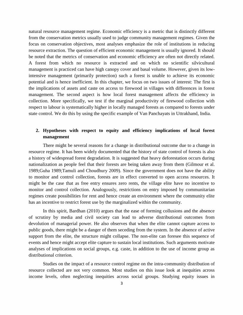
In villages with Van Panchayats, total collection of firewood increases marginally till the

fourth quintile and declines thereafter. Collection from government forest mimics this trend. Van

Panchayat forest is the largest source of firewood and the collection shows a non-linear

relationship. The middle quintiles extract the most from Van Panchayat forests. Collection from

Civil Soyam forests decline with asset holdings. Civil Soyam forests are un-demarcated and un-

protected forests. While collection from owned land increases with quintile, they form a

negligible part of total firewood collection.

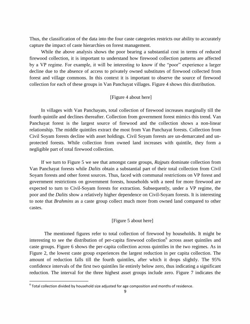
If we turn to Figure 5 we see that amongst caste groups, Rajputs dominate collection from

Van Panchayat forests while Dalits obtain a substantial part of their total collection from Civil

Soyam forests and other forest sources. Thus, faced with communal restrictions on VP forest and

government restrictions on government forests, households with a need for more firewood are

expected to turn to Civil-Soyam forests for extraction. Subsequently, under a VP regime, the

poor and the Dalits show a relatively higher dependence on Civil-Soyam forests. It is interesting

to note that Brahmins as a caste group collect much more from owned land compared to other

castes.


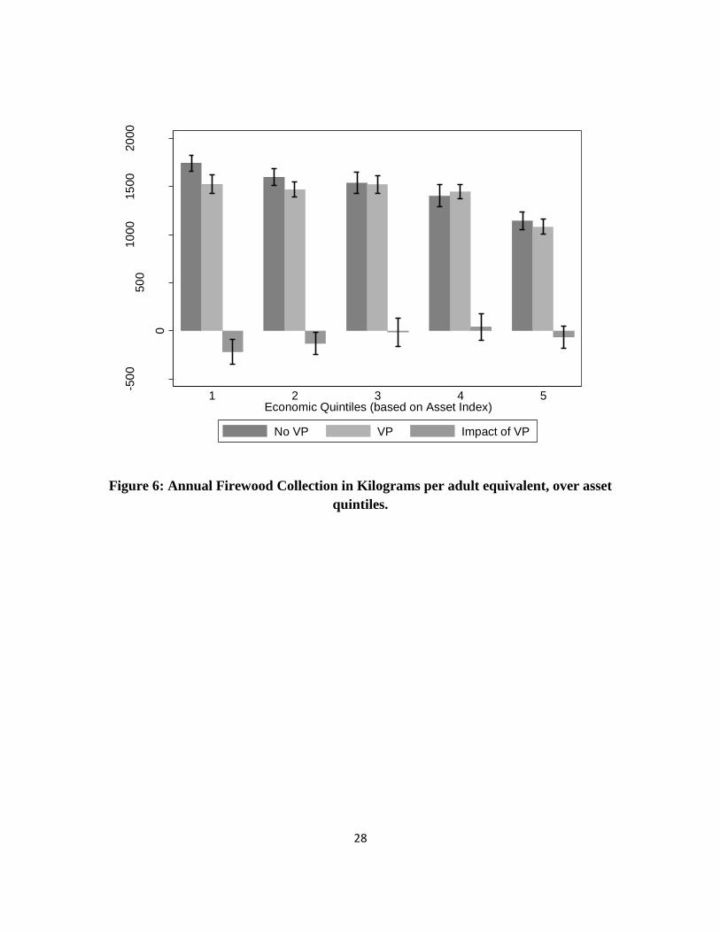
The mentioned figures refer to total collection of firewood by households. It might be

interesting to see the distribution of per-capita firewood collection6 across asset quintiles and

caste groups. Figure 6 shows the per-capita collection across quintiles in the two regimes. As in

Figure 2, the lowest caste group experiences the largest reduction in per capita collection. The

amount of reduction falls till the fourth quintiles, after which it drops slightly. The 95%

confidence intervals of the first two quintiles lie entirely below zero, thus indicating a significant

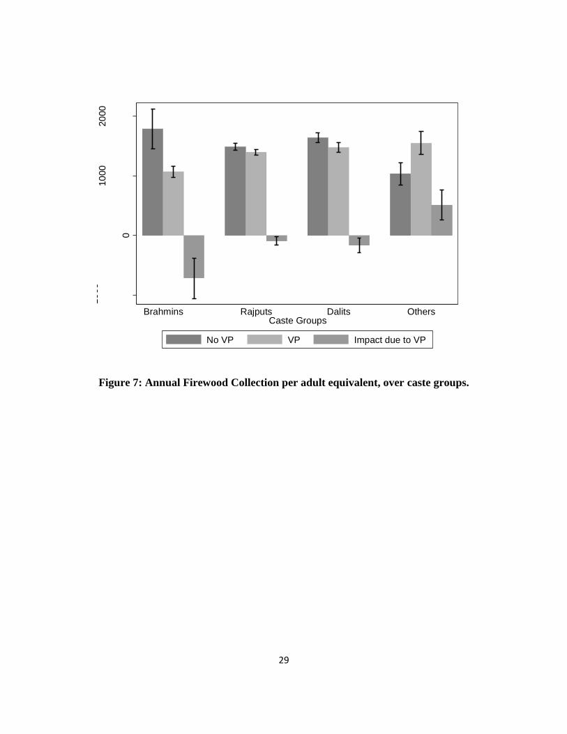
reduction. The interval for the three highest asset groups include zero. Figure 7 indicates the

6 Total collection divided by household size adjusted for age composition and months of residence.

10

differences in per capita collection across caste groups. As in Figure 3, Rajputs experience the

smallest reduction while Brahmins experience the largest reduction. The patterns of per-capita

collection by VP households from different sources (Figure 8 & Figure 9) mimic the patterns in

Figure 4 and Figure 5.





The descriptive statistics discussed above do not establish any causal link between VP

status and the poverty-collection relationship. For example, if Van Panchayats are formed in

villages with better infrastructure, the lower collection of firewood in VP villages might be an

artifact of the fact that villages with better infrastructure are expected to have greater access to

alternatives to firewood. Similarly, if the poor have larger family sizes, it might exaggerate the

impact of Van Panchayat status on firewood collection. In our effort to establish causality, we

take recourse to simple linear regressions with additional controls. We do this by controlling

separately for assets and caste before combining them in a full specification.

[Table 1 about here]

In Table 1, column (1), we start by regressing firewood collection on Van Panchayat

Status, our Asset Index, and the interaction of the two and a host of other controls.7 The

coefficient of the VP variable is negative and significant throughout the specifications. We also

have a number of significant controls such as household size (+) and composition, forest quality

(+), presence of a primary health centre (-) (an indicator of public infrastructure and prosperity in

a village) and availability of the substitute LPG (-). The coefficient of the interaction term

between VP and asset index is the one of interest, but has very low statistical significance in this

specification. The coefficient of the asset index term is, however, negative and significant. Thus

in villages without VP, we have a confirmation of the poverty-environment hypothesis8. The

poor collect more forest resources, in this case firewood, compared to the rich. However, in

column (2), when we add dummies for castes, the coefficient of the interaction term is positive,

indicating that the negative relationship between asset ownership and firewood collection is

dampened in the presence of a VP.

Recall that Figure 2 indicated a non-linear relationship between assets and collection in

VP villages. In column (3) we therefore divide the households into five quintiles to capture non-

linearities that might exist in this relationship. We include dummies for each quintile (the lowest

7 Only two households report no firewood collection. Thus we don’t have a serious problem of censoring.

8The Poverty Environment Hypothesis states that natural resource extraction falls as households become richer.

11

quintile being the omitted group) and interactions of each with the Van Panchayat dummy. This

way we capture the significant reduction in collection by the quintile with the most assets.

Among the interaction terms, it is only a positive interaction between VP and the fourth asset

quintile that is significant (+). These results remain as we add on the caste dummies in column

(4).

In column (5) we include caste dummies and their interaction with VP status while

dropping the asset variables. Brahmins are considered to be the omitted category. The dummies

for Rajput and Dalit are insignificant indicating that these two castes collect firewood in amounts

similar to Brahmins in a non-VP regime. However Other castes consume much less in such a

situation. The interaction terms are highly significant when VP status is interacted with Other

castes while it is only significant at a 10% level when interacted with Dalits and Rajputs. Thus,

as observed in Figure 3, the negative impact of VP on firewood collection is the highest for

Brahmins. However, for reasons mentioned earlier, this result has to be interpreted cautiously.

Brahmins as a group is not unambiguously higher in ritual purity than Rajputs (Guha, 1989).

In specification (6), we allow for interaction of VP status with both asset quintile

dummies as well as caste dummies. In this full specification we replicate all the mentioned

significant results and with higher overall significance.

Till now our analysis was based on the fact that the location of VP villages is exogenous.

However, the history of Van Panchayats points to possibilities that the choice of Van Panchayats

might be endogenous. For example, the fact that the application for Van Panchayats had to be

signed by 66% of adult population (later reduced to 20%) shows that it is likely that the villages

with a homogenous population and strong leadership could apply for the status. To the extent

that these factors also affect firewood collection patterns in a village, non-inclusion of such

village characteristics might led to biased estimates. Since we don’t have historical data about

village conditions prior to VP formation, we use village level fixed effects to control for village

heterogeneity9. However, the use of fixed effects makes it impossible to identify the impact of

village level variables (most importantly, VP (Village)) on firewood collection. However in the

context of this paper we are more interested in the interaction of VP (Village) with asset indices

and caste dummies.


The first two columns of Table 2 provide the fixed effects estimates of specifications

discussed in column (1) and (2) of Table 1. In both specifications, the asset index is negatively

significant while the interaction is positively significant. This reinforces the previous results. In

column (3) and (4) we have fixed effect estimates of a specification similar to column (3) and (4)

9Hausman tests suggest in most cases fixed effects to be the correct specification, as compared to a random effects

model.

12

of Table 2, respectively. The estimates mimic the results obtained from the OLS estimations.

However, in the specifications that involve interaction between caste and VP status (columns (5)

and (6) of Table 2), we don’t find any differential impact across castes. This is different from our

results in the OLS estimations. Column (5) and (6) of Table 1 show Brahmins bearing the largest

burden of reduction in firewood collection. Introduction of fixed effect washes away all the caste

effect we saw earlier. However, the results regarding differential impact across asset quintiles are

robust to introduction of fixed effects.

In Table 3, we consider the adult equivalent per capita firewood collection as the relevant

dependent variable. The set of controls used is similar to the control set in Table 1. It should be

noted that in each of the six specifications in Table 3, household size is negative and significant,

that is, per capita collection falls as household size increases, indicating scale economies in

firewood use. The coefficient of the Van Panchayat dummy is negative and significant,

reinforcing the conservation impact of Van Panchayats. In Column (1) and (2), the coefficient of

the asset index is negative and significant while the coefficient of its interaction with VP dummy

is positive but insignificant. Thus the relationship between asset ownership and collection does

not seem to be statistically different between the two regimes. The share of working age men,

working age women and school going age girls I household I positively related to collection. It

might be interesting to note that share of school going age boys is never significant reflecting

gender differentials if firewood collection work. In order to capture non-linearities in the

relationship between asset ownership and collection, we use dummies for asset quintiles (and

interact them with VP dummy) in column (3) and (4). The asset dummies, with the exception of

the dummy for the fifth quintile, are statistically insignificant. Thus households belonging to the

fifth quintile collect substantially less than other quintiles. However the interaction terms are all

insignificant. The interaction term between the fourth quintile dummy and VP dummy is

significant at a 10% level of significance. Thus results from column (3) and (4) reinforce the

results obtained earlier.


In column (5) we interact caste dummies with VP dummies, that is, we try to see how VP

status changes the collection across caste groups. The caste dummies are all negative and

significant (Brahmins being the omitted category). Thus in a non VP regime, Brahmins collect

the highest, followed by Dalits, Rajputs and Other castes. The interaction terms are all positive

and significant. The coefficient of the interaction term between the Rajput dummy and the VP

dummy has the highest magnitude. This shows that Rajput experience the lowest reduction due

to a shift to VP regime. In column (6) we interact the VP dummy with both caste and asset

quintile dummies. The interaction between the fourth quintile and VP dummy is positive and

significant, indicating that the fourth quintile experiences a significantly lower reduction than

other quintile due to a change in forest regime. The interaction terms of caste and VP status are

13

positive and significant. As in column (5), Rajputs experience the least reduction due to regime

change.

The first two columns of Table 4 provide the fixed effects estimates of specifications

discussed in column (1) and (2) of Table 3. In both specifications, the asset index is negatively

significant while the interaction is positively significant. This is in contrast to the insignificant

coefficients of the interaction terms in OLS estimation. In column (3) and (4) we have fixed

effect estimates of a specification similar to column (3) and (4) of Table 2, respectively. Now the

coefficients of the interaction terms are insignificant for the fifth asset quintile interaction. Thus

the fifth quintile experiences the lowest reduction in collection. However the fifth quintile has

the lowest collection levels in a non VP regime. Thus introduction of VP regime has an

equalizing effect on the distribution favouring the poor in a non-VP regime. However, in the

specifications that involve interaction between caste and VP status (columns (5) and (6) of Table

2), we don’t find any differential impact across castes. This is quite different from our results in

the OLS estimations. Column (5) and (6) of Table 3 showed Brahmins bearing the largest burden

of reduction in firewood collection. Once again, introduction of fixed effect washes away all the

caste effect.


The above results are suggestive of the fact that the poor bear a disproportionate level of

cost in the process of conserving forests. The marginalized caste groups on the other hand don’t

experience additional costs compared to groups at the top of social hierarchy. Introducing fixed

effects ensures that all effects on the caste axis that we obtain under OLS are washed away. Thus

economic disadvantage rather than social disadvantage, condition the costs of conservation borne

by households.

b) Efficiency of firewood production

In this section, we try to test the economic efficiency of different forest governance

regimes. In particular, we want to test if the average productivity of firewood collection from VP

forests with respect to labor is higher than the average productivity of labor in collection from

non-VP forests. On one hand, communitarian regimes have the possibility of decreasing the

average productivity of labor by introducing restriction on collection from nearby forests or by

regulating the nature of lopping. Government Forests, which are often de facto open access

forests, do not have such restrictions. However by reducing firewood collection, communitarian

regimes might facilitate forest regeneration (assuming that the forest was degraded to begin with)

and enhance the biomass availability in the long run. Baland et. al. (2010) showed the

importance of the institution of Van Panchayats in improving the quality of forests measured in

terms of canopy cover, basal area and basal volume. Since both the effects are possible in

14

Uttarakhand, the dominance of one over the other is a question that needs to be tested

empirically.

In this dataset, we have detailed information on the time allocation by different members

of a household on an average day. We explicitly have information on time spent in collection

activities. Using this information we can calculate the total man hours spent by a household in

firewood collection. Unfortunately, we don’t have information about the allocation of firewood

collection time across different forests or different type of forests. Thus, to estimate the marginal

productivity of labour in the two regimes, we restrict our attention to only those villages that

have access to only one kind of forests: either Van Panchayat forests or Non Van Panchayat

forests. Villages that have access to both kinds of forests are dropped from the sample. This

restrict our sample to 46 villages (916 households) of which 9 villages (178 households) have

Van Panchayats. With this sample we try to estimate the firewood production function in both

regimes.


In Table 5, we compare the labour hours allocated to firewood collection by households each

day in the firewood collection season. We find that for every asset quintile and caste group,

households spend more time on collection when they are in a non VP regime. The differences are

higher for the lowest asset group and Dalits. Rajput experience very little reduction in time

allocated. As mentioned earlier, the source of this reduction might be exogenous (due to restrictions

on time spend in forests) or endogenous (restrictions on the kind of trees that can be lopped, mode of

lopping and area where lopping is allowed might reduce the productivity of labour spent on

firewood collection. Reduced productivity will reduce time allocation if we assume the opportunity

cost of time to be unchanged). It might also be the case that VPs improve the quality of forest,

thereby ensuring that a certain quantity of firewood might be collected in less time. This explanation

is based on the assumption that a household has a rather fixed demand of firewood which it tries to

collect efficiently. The analysis that follows tries to disentangle these effects.


Table 6 shows the mean average product of firewood production across different socio-

economic groups for the two regimes. There is no statistically significant difference between the two

regimes except for the fourth quintile and two caste groups: Dalits and Other castes. For these three

groups, the average product is much higher in the VP regimes. Now average productivity can rise

due to increase in productivity (upward shift of the production function) or due to reduction in

15

labour use (the production function remaining unchanged). We know from Table 5, the labour spent

on firewood collection is lower in VP villages. As mentioned earlier, this might be because of

exogenous or endogenous reasons. We try to plot the average product as a function of labour to find

out the source of increase in APL in VP villages.

We use local polynomial regression to non-parametrically plot the relationship between

average product and time spend on firewood collection (Figure 10). We do this separately for the

two regimes. The average product curve for the VP regimes lies entirely below the curve for non-VP

regime. This leads credence to the hypothesis that restriction imposed on nature of extractions (on

the kind of trees that can be lopped or insistence on ecologically sustainable lopping methods)

reduces the returns from labour spent on collection. However the 95% confidence intervals of the

two curves overlap each other at very high and very low values of labour spent. The above figure

does not control for any variable other than labour. We try to control for these using parametric

models.

Let us assume that the production function has a functional form like:

F=A(x)Lα

Where F is the firewood collected, L is labour spent in collection and A is the productivity parameter

which is a function of x. Note that the function A(x) and the parameter α can be different for VP and

non-VP households. The average product is given by:

APL=F/L=A(x)Lα-1

or, log(F/L)=log A(x)+(α-1)log L

Thus we estimate the population regression function:

log (F/L)=b0+ b1VP + b2log L+ b3(VP*log L) + ε

Table 7 has the coefficients estimated for different functional forms. The coefficient of the VP

dummy and it’s interaction with the labour is negative but never significant. Thus everything else

being constant, the average product schedule is identical for VP households and non VP households.

This implies that there is no upward shift in the fuelwood production function due to a shift to VP

regime. Hence the higher average product for VP households that we observe in earlier tables is due

to reduced time spent on firewood collection and not due to productivity shifts. It should be noted

that earlier work by Baland et al. (2010) shows that VP forests are of better quality than non-VP

forests. However, our results are robust to the inclusion (or exclusion) of forest quality as a control.

It is conceivable that the improvement in forest quality does not translate to higher productivity due

to extraction rules that aims to maximize the conservation objective.

16

Note that in the above regressions, we don’t allow controls other than the log of labour for firewood

collection to have differential impact on the log of average product (APL) for the two regimes. In

Table 8, we estimate the functions separately for the two regimes. We test two specifications: one in

which we control for forest quality and the other where we don’t control for forest quality. In

specification (1), coefficients of none of the variables are statistically different between the two

regressions. However the chow test rejects the null hypothesis. In specification (2), we introduce

forest quality as an additional control. In addition to labour, distance to forest has a negative and

significant coefficient for VP regime. However, this is not the case for the non VP regime. Also,

forest quality has a positive and significant effect in the non-VP regime, but not in the VP regime.

This suggests that restricts imposed in VP regimes are not sensitive to forest quality. The overall

Chow test rejects the null hypothesis. In Figure 11, we plot the results obtained in Table 8, holding

variables other than labour constant at their mean values. The average productivity curve of VP

regime lies consistently below that for the non VP regime. This suggests that restrictions imposed in

VP regimes shift the average productivity schedule downwards. However, reduced labour allocation

to firewood collection ensures higher average productivity of labour for VP households compared to

non VP households.

6. Conclusion

In the larger political economy literature, the impact of devolution of power on within-

community distribution of benefits has often been studied and questioned (Dasgupta and Beard

2007; Princen andTiteca 2008). The issue of distributional impact of devolution has more rarely

been studied in the context of natural resource management. While studies have analyzed issues

of inequality and injustice within specific management regimes (Omvedt 1997; Kumar 2002),

comparison has rarely been made across regimes. This specific question achieves great

importance in South Asia as the poor depend heavily on common natural resources for survival

in this region (Jodha 1986;Qureshi and Kumar 2002). South Asia has high levels of economic

and social inequality. In the Hindu majority countries of India and Nepal, social inequality

expresses itself in the form of caste distribution. Thus, this essay tries to understand the

distributional effects of devolution of natural resource management by studying the specific

example of Van Panchayats in Uttarakhand.

In this chapter, we do find some evidence that presence of Van Panchayats leads to

reduced firewood collection by households. The reduction in collection is significantly higher at

the lower end of the household distribution. ‘Poor’ households (i.e. households with low assets)

experience a large reduction in collection in both absolute and proportionate terms. In fact, in

Van Panchayat villages, the relationship between firewood collection and asset holding becomes

positive for the lower half of asset distribution. However, we don’t find such adverse effect on

grounds of caste. Brahmins who are at the top of the social hierarchy, experience the largest

decline in firewood collection, compared to other caste groups when fixed effects are not used.

However, the use of fixed effects wash away all caste effects of the impact of VP management.

17

This result has important implications for policy. While creating communitarian forest

institutions like JFM, government has tried to ensure equity by mandating representation of

marginalized identity groups like Dalits, Other Backward Castes, tribals and women. However,

this study shows that economic status rather than caste is the major axis around which the

differential impact of a communitarian regime is felt. Reservations for Dalits or Backward

Castes might indirectly ensure representation of the poor since such categories are most often

poorer than upper castes. However, ensuring representation of the economically marginalized

might be a more direct way of achieving intra-community equity.

While this paper suggests that community forestry might have adverse distributional

consequences, some issues require further investigation. The initial results in this paper (obtained

using classical regression techniques) are based on the assumption of exogeneity of Van

Panchayat location. However, as villages have to initiate the process of Van Panchayat

formation, the location of VPs might be endogenous. Later, we try to control for such

endogeneity by using village fixed effects. However, in the process of estimation using fixed

effects, we lose out information about the impact of variables defined at village level. To control

for that, we need credible instruments for VP location. Prior to 1947, only British controlled

areas could formally form VPs. Besides this, the Kumaon Association played an important role

in organizing people to assert their forest rights. Thus, even within British controlled areas,

village in Kumaon should have a higher probability of forming VPs. This can be used to create

instruments for VP location. As villagers had to come to Nainital to apply for VP formation, it is

also likely that villages closer to Nainital will have higher chance of forming VPs. We plan to do

further research on this after collecting secondary information to create such instruments.

18

REFERENCES:

Acheson, J. (1988): The Lobster Gangs of Maine. New England Universities Press.

Adhikari, B. (2008): Caste and Social Justice in Common Property Forest Management in Nepal,

Presented at the 16th Annual Conference of European Association of Environmental and

Resource Economists (EAERE), Gothenburg, Sweden.

Agarwal, B. (2001): Participatory Exclusions, Community Forestry, and Gender: An Analysis

for South Asia and a Conceptual Framework," World Development, 29, 1623 -1648.

Agarwal, B. (2007): Inequality, cooperation, and environmental sustainability, Princeton

University Press, Princeton & Oxford and Russel Sage Foundation, New York, chap.

Gender Inequality, Cooperation and Environmental Sustainability, 274-313, editors:

Jean-Marie Baland and Pranab Kumar Bardhan and Samuel Bowles.

Agarwal, R. (1999): “Van Panchayats in Uttrakhand: A Case Study” Economic and Political

Weekly, Vol. 34 (39). 25th

September, 1999. Page 2779-2781

Baland, J. M., Bardhan, P., Das, S. and Mookherjee, D (2010): Forests to the People:

Decentralization and Forest Degradation in the Indian Himalayas, World Development.

38(11), 1642-1656

Bandhyopadhyay, S. and P. Shyamsundar (2004): ``Fuelwood Consumption and Participation in

Community Forestry in India, " World Bank Policy Research Working Paper 3331.

Banerjee, A. (1997): Decentralization and Devolution of Forest Management in Asia and the

Pacific. FAO Working Paper No: APFSOS/WP/21.

ftp://ftp.fao.org/docrep/fao/W7712E/W7712E00.pdf (accessed on 2nd April, 2012)

Banjade, M., H. Luintel, and H. Neupane (2004): "An Action and Learning Process for Social

Inclusion in Community Forestry," Proceedings of the Fourth National Workshop on

Community Forestry, 480-488.

Bardhan, P (2000): “Decentralization and Development: Dilemmas, Trade offs and Safeguards”,

University of California at Berkeley.

Bardhan, P. (2000): Irrigation and Cooperation: An Empirical Analysis of 48 Irrigation

Communities in South India," Economic Development and Cultural Change, 48, 847-

865.

Bardhan, P., M. Ghatak, and A. Karaivanov (2007): Wealth Inequality and Collective Action,"

Journal of Public Economics, 91, 1843 -1874.

Berkes, F. (1986): “Local Level Management and the Commons Problem: A Comparative Study

of Turkish Coastal Fisheries," Marine Policy, 10, 215-229.

ftp://ftp.fao.org/docrep/fao/W7712E/W7712E00.pdf

19

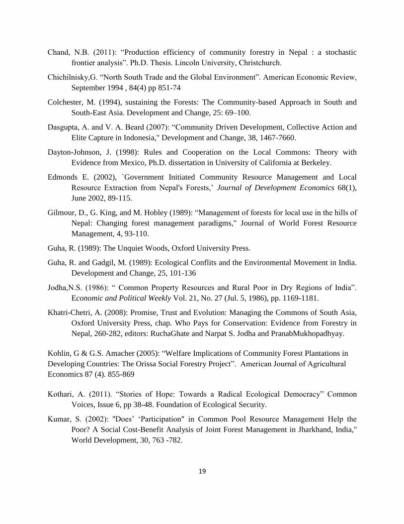
Chand, N.B. (2011): “Production efficiency of community forestry in Nepal : a stochastic

frontier analysis”. Ph.D. Thesis. Lincoln University, Christchurch.

Chichilnisky,G. “North South Trade and the Global Environment”. American Economic Review,

September 1994 , 84(4) pp 851-74

Colchester, M. (1994), sustaining the Forests: The Community-based Approach in South and

South-East Asia. Development and Change, 25: 69–100.

Dasgupta, A. and V. A. Beard (2007): “Community Driven Development, Collective Action and

Elite Capture in Indonesia," Development and Change, 38, 1467-7660.

Dayton-Johnson, J. (1998): Rules and Cooperation on the Local Commons: Theory with

Evidence from Mexico, Ph.D. dissertation in University of California at Berkeley.

Edmonds E. (2002), `Government Initiated Community Resource Management and Local

Resource Extraction from Nepal's Forests,’ Journal of Development Economics 68(1),

June 2002, 89-115.

Gilmour, D., G. King, and M. Hobley (1989): “Management of forests for local use in the hills of

Nepal: Changing forest management paradigms," Journal of World Forest Resource

Management, 4, 93-110.

Guha, R. (1989): The Unquiet Woods, Oxford University Press.

Guha, R. and Gadgil, M. (1989): Ecological Conflits and the Environmental Movement in India.

Development and Change, 25, 101-136

Jodha,N.S. (1986): “ Common Property Resources and Rural Poor in Dry Regions of India”.

Economic and Political Weekly Vol. 21, No. 27 (Jul. 5, 1986), pp. 1169-1181.

Khatri-Chetri, A. (2008): Promise, Trust and Evolution: Managing the Commons of South Asia,

Oxford University Press, chap. Who Pays for Conservation: Evidence from Forestry in

Nepal, 260-282, editors: RuchaGhate and Narpat S. Jodha and PranabMukhopadhyay.

Kohlin, G & G.S. Amacher (2005): “Welfare Implications of Community Forest Plantations in

Developing Countries: The Orissa Social Forestry Project”. American Journal of Agricultural

Economics 87 (4). 855-869

Kothari, A. (2011). “Stories of Hope: Towards a Radical Ecological Democracy” Common

Voices, Issue 6, pp 38-48. Foundation of Ecological Security.

Kumar, S. (2002): ''Does’ ‘Participation" in Common Pool Resource Management Help the

Poor? A Social Cost-Benefit Analysis of Joint Forest Management in Jharkhand, India,"

World Development, 30, 763 -782.

20

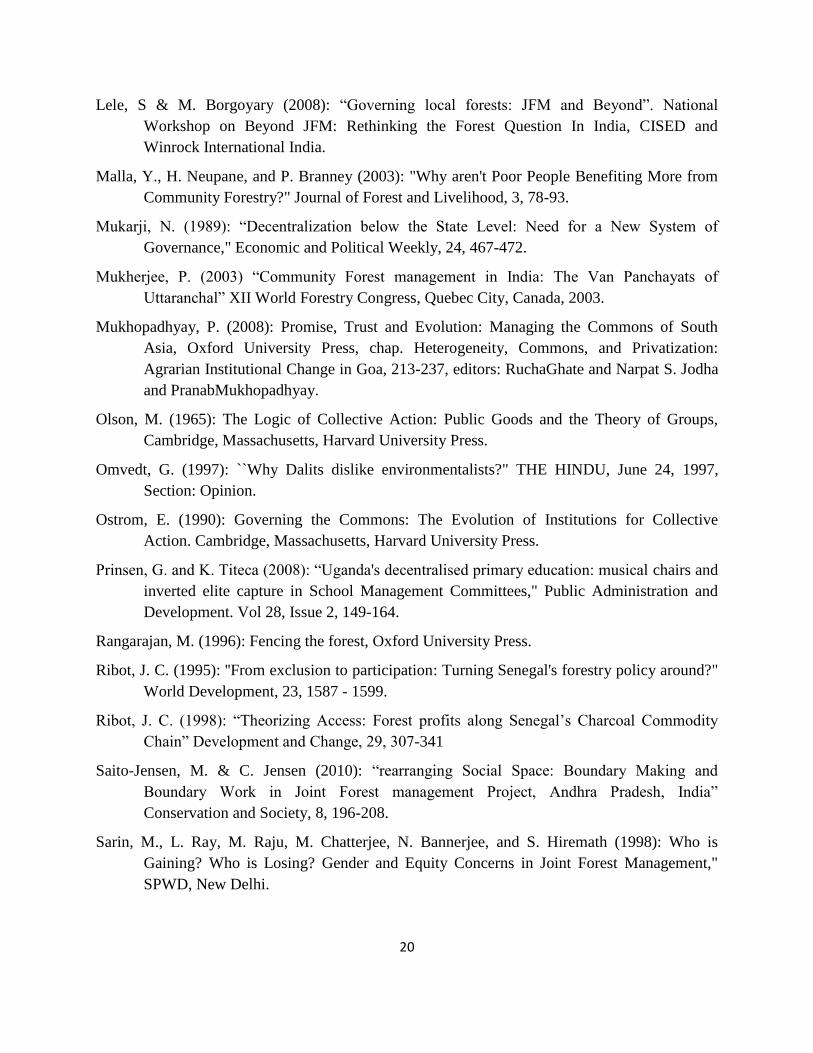
Lele, S & M. Borgoyary (2008): “Governing local forests: JFM and Beyond”. National

Workshop on Beyond JFM: Rethinking the Forest Question In India, CISED and

Winrock International India.

Malla, Y., H. Neupane, and P. Branney (2003): "Why aren't Poor People Benefiting More from

Community Forestry?" Journal of Forest and Livelihood, 3, 78-93.

Mukarji, N. (1989): “Decentralization below the State Level: Need for a New System of

Governance," Economic and Political Weekly, 24, 467-472.

Mukherjee, P. (2003) “Community Forest management in India: The Van Panchayats of

Uttaranchal” XII World Forestry Congress, Quebec City, Canada, 2003.

Mukhopadhyay, P. (2008): Promise, Trust and Evolution: Managing the Commons of South

Asia, Oxford University Press, chap. Heterogeneity, Commons, and Privatization:

Agrarian Institutional Change in Goa, 213-237, editors: RuchaGhate and Narpat S. Jodha

and PranabMukhopadhyay.

Olson, M. (1965): The Logic of Collective Action: Public Goods and the Theory of Groups,

Cambridge, Massachusetts, Harvard University Press.

Omvedt, G. (1997): ``Why Dalits dislike environmentalists?" THE HINDU, June 24, 1997,

Section: Opinion.

Ostrom, E. (1990): Governing the Commons: The Evolution of Institutions for Collective

Action. Cambridge, Massachusetts, Harvard University Press.

Prinsen, G. and K. Titeca (2008): “Uganda's decentralised primary education: musical chairs and

inverted elite capture in School Management Committees," Public Administration and

Development. Vol 28, Issue 2, 149-164.

Rangarajan, M. (1996): Fencing the forest, Oxford University Press.

Ribot, J. C. (1995): ''From exclusion to participation: Turning Senegal's forestry policy around?"

World Development, 23, 1587 - 1599.

Ribot, J. C. (1998): “Theorizing Access: Forest profits along Senegal’s Charcoal Commodity

Chain” Development and Change, 29, 307-341

Saito-Jensen, M. & C. Jensen (2010): “rearranging Social Space: Boundary Making and

Boundary Work in Joint Forest management Project, Andhra Pradesh, India”

Conservation and Society, 8, 196-208.

Sarin, M., L. Ray, M. Raju, M. Chatterjee, N. Bannerjee, and S. Hiremath (1998): Who is

Gaining? Who is Losing? Gender and Equity Concerns in Joint Forest Management,"

SPWD, New Delhi.

http://en.wikipedia.org/wiki/World_Forestry_Congress

21

Sarin, M; Singh, N.M.; Sundar,N&Bhogal, R.K. (2003): Devolution as a threat to Democratic

Decision-making in Forestry? Findings from Three Sates in India.WorkingPaper 197,

Overseas Development Institute.

Sakurai, T; Rayamajhi, S; Pokharel, R.K. and Otsuka, K. (2004): “Efficiency of Timber

production in Community and Private Forestry in Nepal”. Environment and Development

Economics, 9: 539-561

Sethi, Rajiv and E. Somanathan.1996. "The evolution of social norms in common property

resource use," The American Economic Review, 86:4, pp. 766-788

Singh, K.D., Sinha, B. & Mukherjee, S.D. (2005) Exploring options for Joint Forest management

(JFM) in India. Rome, FAO and Washington DC, World Bank.

Somanathan, E, R. Prabhakar& B.S. Mehta (2005): “Does Decentralization work? Forest

Conservation in the Himalayas”.BREAD Working Paper No. 096.

Sundar, N. (2000): Unpacking the `Joint' in Joint Forest Management," Development and

Change, 31, 255-279.

Tamuli, J & S. Chowdhury: ``RE looking at forest policies in Assam: facilitating reserved forests

as de facto open access”. MPRA Paper No. 29560, posted 11. May 2011 / 09:37

Timsina, N. P. (2003): Promoting social justice and conserving montane forest environments: A

case study of Nepal's community forestry programme," The Geographical Journal, 169,

236-242.

22

Figures:

23

Figure 1: Map of Uttarakhand.

[The district names and their boundaries are those of the modern day Indian state of Uttrakhand.

However the colour shades refer to the administrative divisions of the region during the period

1815-1949.]

24

Figure 2: Firewood Collection for different economic groups (quintiles)

in Van Panchayat and Non-Van Panchayat villages.

-20

00

0

20

00

40

00

60

00

Mea

n A

nn

ua

l F

irew

ood

Colle

ction

(K

gs)

1 2 3 4 5Economic Quintiles (based on Asset Index)

No VP VP Impact of VP

25

Figure 3: Firewood Collection for different caste groups

in Van Panchayat and Non-Van Panchayat villages.

-50

00

0

50

00

10

00

0

Mea

n A

nn

ua

l F

irew

ood

Colle

ction

(K

gs)

Brahmins Rajputs Dalits OthersCaste Groups

No VP VP Impact due to VP

26

FIGURE 4: FIREWOOD COLLECTION FROM DIFFERENT SOURCES (ACROSS ASSET QUINTILES) IN VP

VILLAGES

0

10

00

20

00

30

00

Kilo

gra

ms o

f F

ire

wo

od

FW Bought Own Land Commons FD CS VP Oth Forest

Source of Firewood for VP households

27

Figure 5: Firewood Collection from different sources (across caste groups) in VP Villages

0

500

1000

1500

2000

2500

Kilo

gra

ms o

f F

irew

ood (

Per

Capita)


1st bar:Brahmins 2nd bar:Rajputs 3rd bar:Dalits 4th bar:Others

28

Figure 6: Annual Firewood Collection in Kilograms per adult equivalent, over asset

quintiles.

-50

0

0

50

010

00

15

00

20

00

Mea

n A

nn

ua

l F

irew

ood

Colle

ction

per

cap

ita

(K

gs)

1 2 3 4 5Economic Quintiles (based on Asset Index)

No VP VP Impact of VP

29

Figure 7: Annual Firewood Collection per adult equivalent, over caste groups.

-10

00

0

10

00

20

00

Mea

n A

nn

ua

l F

irew

ood

Colle

ction

(K

gs)

Brahmins Rajputs Dalits OthersCaste Groups

No VP VP Impact due to VP

30

Figure 8: Per adult equivalent collection of firewood (Kilograms per year) for VP

households, over asset quintiles.

0

20

040

060

080

0

Kilo

gra

ms o

f F

ire

wo

od


31

Figure 9: Per adult equivalent collection of firewood (Kilograms per year) for VP

households, over caste groups.

0

200

400

600

800

1000

Kilo

gra

ms o

f F

irew

ood (

Per

Capita)


1st bar:Brahmins 2nd bar:Rajputs 3rd bar:Dalits 4th bar:Others

Figure 10: Relationship between Average Product and Labour spent on firewood collection. Curve fitted non-parametrically using locally weighted

scatter plot smoothing.

Figure 11: A) Corrsponding to Column (1) of Table 8

Figure 11: B) Corresponding to column (2) in Table (8)

Figure 11: Graphical Respresentation of Table (8)

(Variables other than Labour held constant at their means)

Tables

(1) (2) (3) (4) (5) (6)Dependent Variable: Annual Firewood Collection in Kilograms

VP (Village) -741.33*** -753.52*** -807.15*** -792.93*** -1635.11*** -1926.52***(3.33) (3.42) (3.96) (3.85) (2.69) (3.35)

Asset Index -4030.89*** -3912.15***(5.78) (5.62)

VP (Village) × Asset Index 1197.46 1308.40*(1.61) (1.85)

Second Asset Quintile -55.02 -44.51 -96.59(0.32) (0.25) (0.57)

Third Asset Quintile -296.30 -281.08 -339.46(1.10) (1.03) (1.23)

Fourth Asset Quintile -372.72 -347.22 -405.94(1.44) (1.35) (1.51)

Fifth Asset Quintile -1236.84*** -1188.03*** -1245.46***(3.54) (3.39) (3.39)

VP(Village) × Second Asset Quintile 169.07 143.70 198.69(0.71) (0.60) (0.85)

VP(Village) × Third Asset Quintile 426.09 421.09 490.94(1.35) (1.33) (1.54)

VP(Village) × Fourth Asset Quintile 625.96** 641.98** 722.67**(2.02) (2.11) (2.25)

VP(Village) × Fifth Asset Quintile 349.28 379.11 495.73(0.94) (1.04) (1.25)

Rajput 293.57 326.05 -407.80 -439.96(1.07) (1.24) (0.73) (0.87)

Dalit 380.67 448.02 -192.21 -325.94(1.18) (1.42) (0.32) (0.58)

Other Castes -97.83 -136.44 -1829.92*** -1510.12***(0.39) (0.53) (3.00) (2.69)

VP (Village) × Rajput 1172.34* 1116.13**(1.98) (2.11)

VP (Village) × Dalit 1134.34* 1173.59*(1.77) (1.91)

VP (Village) × Other Caste 2066.88*** 1780.43***(3.06) (2.96)

Adjusted Household Size 668.76*** 661.46*** 661.76*** 653.72*** 605.23*** 654.65***(12.92) (12.71) (13.18) (12.96) (11.93) (12.94)

Share of Men (> 16 yrs.) 945.92*** 902.62** 812.50** 760.72** 959.70*** 689.62**(2.67) (2.51) (2.24) (2.09) (2.76) (1.99)

Share of Women (> 16 yrs.) 1468.95*** 1377.59*** 1321.73*** 1215.85*** 1429.02*** 1167.77***(4.18) (4.01) (3.69) (3.49) (4.16) (3.44)

Share of Boys (≥6 yrs. & ≤ 16 yrs.) 976.17* 880.53* 908.29* 793.81 1287.58** 751.92(1.97) (1.79) (1.82) (1.62) (2.59) (1.56)

Share of Girls (≥6 yrs. & ≤ 16 yrs.) 1968.18*** 1864.99*** 1892.95*** 1767.47*** 2278.29*** 1718.53***(4.32) (4.04) (4.01) (3.71) (5.04) (3.75)

Male Headed Household 302.00** 273.01* 342.65** 305.49** 503.32*** 290.72**(2.18) (1.98) (2.42) (2.17) (3.51) (2.10)

Education of Household Head 4.25 5.56 -2.01 0.16 -23.10 1.65(0.30) (0.37) (0.14) (0.01) (1.46) (0.11)

No. of Private Trees 0.59 0.71 0.44 0.60 -0.31 0.64(0.50) (0.60) (0.37) (0.52) (0.29) (0.58)

Per Capita Forest Area -65.22 -28.31 -83.81 -37.66 -60.06 3.37(1.06) (0.41) (1.33) (0.54) (0.86) (0.05)

Forest Quality: Basal Area 7.64** 7.02* 8.30** 7.55* 7.92** 6.60*(2.11) (1.81) (2.22) (1.89) (2.14) (1.85)

Distance to Forest -38.05 -45.30 -39.89 -47.69 -33.05 -31.24(0.45) (0.57) (0.45) (0.57) (0.37) (0.39)

Altitude of Village 0.12 0.15 0.19 0.22 0.16 0.16(0.43) (0.53) (0.63) (0.73) (0.50) (0.52)

Electricity in Village -155.04 -165.59 -192.84 -207.56 -202.50 -217.67(0.56) (0.59) (0.67) (0.71) (0.66) (0.73)

PHC in Village -521.81*** -529.67*** -574.03*** -581.74*** -671.32*** -592.73***(3.68) (3.72) (4.00) (3.97) (4.88) (4.25)

Link to Motorable Road -59.59 -52.31 -5.53 0.98 -4.88 -26.81(0.32) (0.28) (0.03) (0.01) (0.02) (0.15)

Availability of LPG -386.52*** -374.20*** -419.40*** -404.34*** -526.27*** -382.23***(2.80) (2.67) (2.89) (2.75) (3.70) (2.70)

Constant 2647.01*** 2414.09*** 2157.00*** 1906.93** 2427.97** 2855.72***(3.51) (2.80) (2.76) (2.18) (2.38) (2.93)

Observations 1552 1552 1552 1552 1555 1552R2 0.35 0.35 0.35 0.35 0.33 0.36

Absolute t statistics in parentheses. ∗p < .10, ∗ ∗ p < .05, ∗ ∗ ∗p < .01

Table 1: Linear Regressions (t statistics are calculated using cluster robust standard errors)

(1) (2) (3) (4) (5) (6)Dependent Variable: Annual Firewood Collection in Kilograms

Asset Index -3161.59*** -3149.44***(4.83) (4.78)

VP (Village) × Asset Index 1596.39** 1639.58**(1.98) (2.02)

Second Asset Quintile 51.69 50.19 46.62(0.27) (0.26) (0.24)


Fourth Asset Quintile -46.45 -47.89 -51.04(0.20) (0.20) (0.22)




VP(Village) × Fourth Asset Quintile 628.68** 625.09** 629.15**(2.01) (1.99) (1.99)

VP(Village) × Fifth Asset Quintile 543.80 545.02 564.19*(1.62) (1.61) (1.65)

Rajput -7.18 23.19 -242.04 -204.15(0.03) (0.09) (0.59) (0.50)

Dalit -23.85 23.54 -175.47 -216.14(0.09) (0.09) (0.43) (0.53)

Other Castes -385.15 -308.73 -222.08 -13.23(0.90) (0.72) (0.25) (0.02)

VP (Village) × Rajput 364.44 385.72(0.70) (0.74)

VP (Village) × Dalit 340.88 439.82(0.62) (0.80)

VP (Village) × Other Caste -282.66 -299.25(0.28) (0.30)

Adjusted Household Size 630.21*** 627.89*** 615.56*** 613.90*** 585.10*** 612.57***(18.91) (18.77) (18.33) (18.23) (17.87) (18.16)

Share of Men (> 16 yrs.) 726.33* 732.58* 633.41 636.94 755.62* 623.44(1.72) (1.73) (1.49) (1.50) (1.77) (1.46)

Share of Women (> 16 yrs.) 1250.13*** 1235.35*** 1095.89** 1082.58** 1259.96*** 1060.22**(2.79) (2.76) (2.44) (2.41) (2.78) (2.36)

Share of Boys (≥6 yrs. & ≤ 16 yrs.) 406.69 409.08 389.92 388.11 650.39 374.81(0.76) (0.76) (0.72) (0.72) (1.20) (0.69)


Male Headed Household 238.16 233.96 275.67* 269.89* 388.64** 268.91*(1.47) (1.44) (1.70) (1.66) (2.40) (1.65)

Education of Household Head 11.64 11.57 5.21 5.58 -5.92 5.97(0.83) (0.82) (0.37) (0.40) (0.43) (0.42)


Constant 2166.71*** 2202.50*** 1769.74*** 1780.76*** 1795.10*** 1831.66***(4.93) (4.50) (4.01) (3.61) (3.67) (3.69)

Observations 1552 1552 1552 1552 1555 1552R2 0.22 0.22 0.22 0.23 0.20 0.23Adjusted R2 0.17 0.17 0.18 0.17 0.15 0.17


Table 2: Linear Regressions with Village Fixed Effects

(1) (2) (3) (4) (5) (6)Dependent Variable: Annual Firewood Collection in Kilograms per adult equivalent.

VP (Village) -165.94** -171.87*** -178.30*** -177.61*** -652.53*** -715.18***(2.55) (2.71) (2.84) (2.82) (5.57) (5.67)

Asset Index -1032.56*** -1017.44***(5.57) (5.41)

VP (Village) × Asset Index 227.01 262.97(1.06) (1.28)

Second Asset Quintile -19.83 -18.94 -41.56(0.43) (0.40) (0.90)


Fourth Asset Quintile -104.16 -102.06 -124.79*(1.50) (1.43) (1.83)




VP(Village) × Fourth Asset Quintile 128.68 134.83 164.00**(1.59) (1.65) (2.05)

VP(Village) × Fifth Asset Quintile 71.98 84.21 128.32(0.68) (0.82) (1.14)

Rajput 72.53 86.30 -277.34*** -285.81***(0.74) (0.90) (3.08) (3.12)

Dalit 78.86 99.50 -215.37** -252.02**(0.76) (0.98) (2.05) (2.23)

Other Castes -5.97 -14.60 -758.38*** -673.80***(0.05) (0.12) (6.56) (6.03)

VP (Village) × Rajput 556.98*** 545.07***(4.90) (4.90)

VP (Village) × Dalit 505.85*** 517.80***(3.93) (3.72)

VP (Village) × Other Caste 929.03*** 853.81***(5.39) (5.54)

Adjusted Household Size -179.53*** -181.21*** -181.73*** -183.67*** -196.20*** -183.05***(12.76) (12.96) (12.54) (12.69) (15.15) (13.32)

Share of Men (> 16 yrs.) 353.27*** 348.56*** 319.40** 312.87** 351.23*** 280.78**(2.87) (2.92) (2.53) (2.58) (2.93) (2.39)

Share of Women (> 16 yrs.) 712.73*** 694.50*** 677.66*** 655.04*** 700.77*** 635.85***(4.49) (4.41) (4.16) (4.06) (4.49) (4.00)

Share of Boys (≥6 yrs. & ≤ 16 yrs.) 278.32 261.91 262.35 240.71 366.73** 225.15(1.60) (1.55) (1.55) (1.47) (2.15) (1.37)


Male Headed Household 33.23 27.26 47.72 39.30 85.30* 31.50(0.79) (0.64) (1.11) (0.90) (1.95) (0.79)

Education of Household Head 3.13 3.33 0.89 1.31 -4.29 2.05(0.75) (0.80) (0.21) (0.31) (0.97) (0.50)


Per Capita Forest Area -9.56 -1.64 -16.65 -5.94 -0.96 14.84(0.45) (0.07) (0.71) (0.25) (0.05) (0.78)

Forest Quality: Basal Area 1.84** 1.73* 2.02** 1.87** 1.76** 1.40*(2.18) (1.98) (2.27) (2.04) (2.13) (1.79)

Distance to Forest 4.04 2.35 3.78 1.82 8.49 8.95(0.16) (0.10) (0.14) (0.07) (0.35) (0.42)

Altitude of Village 0.09 0.09 0.10 0.11 0.08 0.08(1.03) (1.04) (1.18) (1.19) (1.06) (1.05)

Electricity in Village -90.00 -90.92 -101.35 -103.15 -103.05 -107.82(1.16) (1.16) (1.24) (1.25) (1.21) (1.30)

PHC in Village -157.40*** -158.82*** -172.05*** -173.46*** -198.29*** -178.74***(3.12) (3.19) (3.36) (3.39) (4.41) (4.14)

Link to Motorable Road 10.43 12.49 25.27 27.30 16.74 11.88(0.21) (0.25) (0.48) (0.53) (0.33) (0.25)

Availability of LPG -115.15*** -112.20*** -126.01*** -122.00*** -147.21*** -109.45***(2.87) (2.77) (3.01) (2.90) (3.77) (2.80)

Constant 1881.21*** 1824.20*** 1753.42*** 1687.44*** 2017.57*** 2132.77***(7.69) (6.87) (6.99) (6.32) (7.81) (8.47)

Observations 1552 1552 1552 1552 1555 1552R2 0.32 0.32 0.32 0.32 0.31 0.34


Table 3: Linear Regressions on firewood collection per adult equivalent. (t statistics are calculated using cluster robust standard errors)

(1) (2) (3) (4) (5) (6)Asset Index -836.64*** -844.56***

(4.39) (4.41)VP (Village) × Asset Index 465.36** 479.52**

(1.99) (2.03)Second Asset Quintile -6.01 -7.38 -9.40

(0.11) (0.13) (0.17)Third Asset Quintile 4.24 2.72 0.78

(0.07) (0.04) (0.01)Fourth Asset Quintile -40.29 -43.03 -43.41

(0.59) (0.63) (0.63)Fifth Asset Quintile -244.17*** -247.58*** -250.04***

(3.25) (3.27) (3.28)VP(Village) × Second Asset Quintile 35.49 36.43 36.23

(0.42) (0.43) (0.42)VP(Village) × Third Asset Quintile 94.43 95.01 97.31

(1.06) (1.07) (1.09)VP(Village) × Fourth Asset Quintile 147.19 149.00 149.18

(1.61) (1.63) (1.62)VP(Village) × Fifth Asset Quintile 176.27* 180.17* 181.85*

(1.80) (1.83) (1.82)Rajput -26.06 -17.81 -163.21 -152.17

(0.36) (0.24) (1.36) (1.27)Dalit -43.79 -33.62 -143.85 -159.14

(0.56) (0.43) (1.20) (1.34)Other Castes -55.50 -44.21 -121.44 -68.11

(0.44) (0.35) (0.47) (0.27)VP (Village) × Rajput 215.05 219.33

(1.41) (1.45)VP (Village) × Dalit 183.71 215.05

(1.15) (1.35)VP (Village) × Other Caste 84.18 66.03

(0.29) (0.22)Adjusted Household Size -190.26*** -190.57*** -193.96*** -194.17*** -201.64*** -194.57***

(19.63) (19.58) (19.80) (19.76) (21.21) (19.78)Share of Men (> 16 yrs.) 252.98** 256.29** 233.26* 236.18* 261.00** 231.58*

(2.06) (2.08) (1.88) (1.90) (2.10) (1.86)Share of Women (> 16 yrs.) 653.77*** 654.66*** 621.54*** 622.42*** 661.18*** 617.05***

(5.02) (5.02) (4.75) (4.75) (5.03) (4.70)Share of Boys (≥6 yrs. & ≤ 16 yrs.) 79.62 83.65 80.51 84.10 152.09 85.63

(0.51) (0.54) (0.51) (0.53) (0.97) (0.54)Share of Girls (≥6 yrs. & ≤ 16 yrs.) 442.90*** 444.41*** 441.11*** 441.97*** 496.89*** 431.35***

(2.87) (2.87) (2.83) (2.83) (3.20) (2.76)Male Headed Household 7.60 8.70 19.08 19.77 48.03 19.07

(0.16) (0.18) (0.40) (0.42) (1.02) (0.40)Education of Household Head 4.38 4.08 2.48 2.27 -0.34 2.45

(1.07) (0.99) (0.61) (0.55) (0.08) (0.60)No. of Private Trees 0.08 0.06 0.01 -0.00 -0.19 -0.01

(0.30) (0.23) (0.05) (0.00) (0.73) (0.03)Constant 1907.19*** 1935.22*** 1810.80*** 1831.63*** 1842.15*** 1857.24***

(14.92) (13.58) (14.06) (12.75) (12.96) (12.83)Observations 1552 1552 1552 1552 1555 1552R2 0.28 0.28 0.28 0.28 0.27 0.28


Table 4: Regressions with Village fixed effects on firewood collection per adult equivalent.

Non VP VP p-value for test of equality(Adjusted Wald Test)

Asset Quintiles1 8.45 (0.27) 5.80 (1.11) 0.02**2 8.59 (0.33) 6.70 (0.59) 0.01**3 8.34 (0.42) 6.68 (0.50) 0.02**4 8.93 (0.43) 6.35 (0.35) 0.00***5 8.39 (0.36) 6.51 (0.67) 0.02**

CasteBrahmins 9.34 (1.07) 6.40 (0.51) 0.03**Rajputs 8.47 (0.26) 7.41 (0.39) 0.03**Dalits 8.58 (0.26) 5.53 (0.40) 0.00***Others 7.91 (0.00) 5.16 (0.44) 0.01**

Total Sample: 8.53 (0.22) 6.47 (0.25) 0.00***Note: The numbers in the parenthesis denote standard errors (corrected for clustering)

The third columns show the t-statistic for the equality of means test.

Table 5: Labour Allocated per household to Firewood Collection during an average day in the firewood collection season.

Non VP VP p-value for test of equality(Adjusted Wald Test)

Asset Quintiles1 887.81 (33.90) 989.49 (127.76) 0.442 804.99 (27.49) 897.54 (84.26) 0.33 828.04 (38.64) 854.12 (78.96) 0.764 726.96 (42.83) 878.42 (47.45) 0.02**5 672.86 (42.87) 802.26 (90.95) 0.2

CasteBrahmins 715.94 (65.92) 752.81 (59.78) 0.68Rajputs 797.16 (20.10) 830.93 (59.47) 0.58Dalits 846.50 (34.25) 991.53 (59.49) 0.04**Others 566.35 (0.00) 1008.47 (126.50) 0.04**

Total Sample: 800.74 (17.53) 878.37 (43.43) 0.10*Note: The numbers in the parenthesis denote standard errors (corrected for clustering)

The third columns show the t-statistic for the equality of means test.

Table 6: Average Product of Firewood Collection(=Annual Firewood Collection/ Time Spent by household on an average day in firewood collection season).

(1)

(2)

(3)

(4)

(5)

(6)

Dep

end

ent

Vari

ab

le:log(A

PL

)D

um

my:

VP

hou

seh

old

-0.0

86

-0.0

82

-0.1

00

-0.0

91

-0.0

95

-0.0

83

(0.6

3)

(0.6

1)

(0.6

5)

(0.5

6)

(0.6

3)

(0.5

3)

log

(fire

wood

Lab

ou

r)-0

.691

-0.6

99

-0.7

1(1

9.7

2)*

**

(19.0

2)*

**

(19.4

4)*

**

Inte

ract

ion

:lo

g(fi

rew

ood

lab

ou

r)×

VP

Hou

seh

old

Du

mm

y-0

.047

-0.0

63

-0.0

37

(0.7

2)

(0.9

)(0

.53)

log

(Age

Ad

just

edF

irew

ood

Lab

ou

r)-0

.687

-0.6

92

-0.7

03

(20.3

4)*

**

(19.3

6)*

**

(19.6

4)*

**

Inte

ract

ion

:lo

g(A

ge

Ad

just

edF

irew

ood

Lab

ou

r)×

VP

Hou

seh

old

Du

mm

y-0

.05

-0.0

67

-0.0

43

(0.7

7)

(0.9

7)

(0.6

1)

log

(Dis

tan

ceto

Fore

st)

-0.0

92

-0.1

12

-0.0

96

-0.1

15

(1.4

9)

(1.9

0)*

(1.5

4)

(1.9

6)*

*lo

g(P

erC

ap

ita

Fore

stA

rea)

-0.0

29

-0.0

24

-0.0

28

-0.0

24

(1.5

7)

(1.2

4)

(1.5

7)

(1.2

4)

log

(Basa

lA

rea)

0.2

38

0.2

38

(2.6

0)*

*(2

.60)*

*lo

g(A

ltit

ud

eof

Fore

st)

0.1

74

-0.0

83

0.1

84

-0.0

75

(0.8

5)

(0.3

4)

(0.9

)(0

.31)

Con

stant

7.9

89

7.9

96.7

09

7.7

98

6.6

31

7.7

28

(107.4

2)*

**

(114.1

8)*

**

(4.3

2)*

**

(4.8

3)*

**

(4.2

9)*

**

(4.7

9)*

**

Ob

serv

ati

on

s916

916

857

857

857

857

R2

0.4

80.4

80.4

90.5

0.4

90.5

Tab

le7:

Rel

ati

on

ship

bet

wee

nA

ver

age

pro

du

ctiv

ity

of

lab

ou

ran

dla

bou

rh

ou

rsC

lust

erR

ob

ust

Sta

nd

ard

Err

ors

inp

are

nth

esis

Dep

end

ent

Vari

ab

le:

log

(APL

)(1

)(2

)V

PN

on

VP

t-te

stV

PN

on

VP

t-te

stlo

g(fi

rew

ood

Lab

ou

r)-0

.756

-0.6

98

0.8

4-0

.754

-0.7

12

0.6

1(1

2.2

3)*

**

(18.8

2)*

**

(12.0

6)*

**

(19.2

5)*

**

log

(Dis

tan

ceto

Fore

st)

-0.2

55

-0.0

84

1.6

3-0

.242

-0.0

87

1.4

7(3

.10)*

**

(1.1

7)

(2.6

7)*

**

(1.3

6)

log

(Per

Cap

ita

Fore

stA

rea)

-0.0

11

-0.0

30.5

6-0

.003

0.0

02

0.1

7(1

.00)

(0.9

4)

(0.1

5)

(0.1

)lo

g(B

asa

lA

rea)

-0.1

23

0.3

44

2.3

6(0

.65)

(3.7

5)*

**

log

(Alt

itu

de

of

Fore

st)

0.7

32

0.1

49

1.5

91.0

78

-0.1

12.1

5(2

.43)*

*(0

.63)

(2.0

1)*

*(0

.46)

Con

stant

2.3

66.8

94

1.5

90.1

47.5

81.9

9(1

.00)

(3.8

3)*

**

(0.0

4)

(4.5

6)*

**

Ob

serv

ati

on

s139

718

139

718

R2

0.6

20.4

50.6

20.4

7C

how

Tes

t(p

-valu

e)0.0

00.0

0

Tab

le8:

Rel

atio

nsh

ipb

etw

een

Ave

rage

pro

duct

ivit

yof

lab

our

and

lab

our

hou

rsusi

ng

aflex

ible

funct

ional

form

tenure and forest management in india: impacts on … and forest management ... documented cases of...

Documents