temporal scales, trade-offs, and functional responses in red deer habitat selection

Ecology, 90(3), 2009, pp. 699–710� 2009 by the Ecological Society of America

Temporal scales, trade-offs, and functional responsesin red deer habitat selection

INGER MAREN RIVRUD GODVIK,1 LEIF EGIL LOE,1 JON OLAV VIK,1,3 VEBJØRN VEIBERG,1,2 ROLF LANGVATN,2

AND ATLE MYSTERUD1,4

1Centre for Ecological and Evolutionary Synthesis (CEES), Department of Biology, University of Oslo, P.O. Box 1066 Blindern,N-0316 Oslo, Norway

2Norwegian Institute for Nature Research, Tungasletta 2, N-7085 Trondheim, Norway

Abstract. Animals selecting habitats often have to consider many factors, e.g., food andcover for safety. However, each habitat type often lacks an adequate mixture of these factors.Analyses of habitat selection using resource selection functions (RSFs) for animalradiotelemetry data typically ignore trade-offs, and the fact that these may change duringan animal’s daily foraging and resting rhythm on a short-term basis. This may lead to changesin the relative use of habitat types if availability differs among individual home ranges, calledfunctional responses in habitat selection. Here, we identify such functional responses and theirunderlying behavioral mechanisms by estimating RSFs through mixed-effects logisticregression of telemetry data on 62 female red deer (Cervus elaphus) in Norway. Habitatselection changed with time of day and activity, suggesting a trade-off in habitat selectionrelated to forage quantity or quality vs. shelter. Red deer frequently used pastures offeringabundant forage and little canopy cover during nighttime when actively foraging, whilespending much of their time in forested habitats with less forage but more cover duringdaytime when they are more often inactive. Selection for pastures was higher when availabilitywas low and decreased with increasing availability. Moreover, we show for the first time thatin the real world with forest habitats also containing some forage, there was both increasingselection of pastures (i.e., not proportional use) and reduced time spent in pastures (i.e., notconstant time use) with lowered availability of pastures within the home range. Our studydemonstrates that landscape-level habitat composition modifies the trade-off between foodand cover for large herbivorous mammals. Consequently, landscapes are likely to differ intheir vulnerability to crop damage and threat to biodiversity from grazing.

Key words: Cervus elaphus; habitat selection; large mammals; mixed-effects logistic regression;Norway; red deer; resource selection functions; resource use; trade-offs; ungulates.

INTRODUCTION

Habitat selection is an important component of the

ecology of a species (Rosenzweig 1981), and is frequent-

ly defined as the disproportionate use of habitat types

(Johnson 1980). Four hierarchical orders of selection are

identified based on what spatial scale use and availabil-

ity are measured (Johnson 1980, Senft et al. 1987). At

the within-home-range scale, habitat selection is usually

linked to the animal’s daily foraging and resting

rhythms, in contrast to selection of home ranges at

broader scales, which is often linked to dispersal

processes or seasonal migrations (Morris 1987). In the

following, we focus on the within-home-range scale.

When animals choose a habitat, they often have to

consider many factors, such as forage quality and

availability, shelter, and potential predators (Sih 1980,

Werner et al. 1983). Each habitat type may not always

contain an adequate mixture of these factors (Orians

and Wittenberger 1991). The resulting choice of habitat

is thus the outcome of trade-offs between the costs and

benefits perceived by the animal (Lima and Dill 1990,

Mysterud and Ims 1998). A common trade-off often

faced by many large mammals takes place when exposed

habitats provide the best forage, while closed habitats

provide shelter against harsh weather and/or predators.

How the trade-off affects the individuals may vary with

season, time of day, and weather conditions, and also

with the animal’s sex, age, and daily activity (Beier and

McCullough 1990, Manly et al. 2002).

One of numerous methods available for investigating

habitat selection is resource selection functions (RSFs),

defined as any function proportional to the probability

of use of a resource unit or area by an animal (Manly et

al. 2002). These sets of methods, commonly logistic

regression (Johnson et al. 2000, Boyce et al. 2002,

Nielsen et al. 2002, Boyce et al. 2003), have been applied

in studies of habitat selection across a diverse range of

Manuscript received 26 March 2008; revised 3 June 2008;accepted 16 June 2008. Corresponding Editor: T. J. Valone.

3 Present address: Centre for Integrative Genetics (CI-GENE), Norwegian University of Life Sciences, P.O. Box5003, N-1432 As, Norway.

4 Corresponding author. E-mail: [email protected]

699

species, from Pileated Woodpeckers (Dryocopus pileatus;

Lemaitre and Villard 2005) to grizzly bears (Ursus

arctos; Nielsen et al. 2002). Within an animal’s home

range, locations for resource use by the individual are

averages over the period when the data are collected,

and the typical advice given is that the selection times

should be kept as short as possible because the habitats

may change (Manly et al. 2002), e.g., between seasons.

However, such approaches ignore how trade-offs may

change during an animal’s daily foraging and resting

rhythm on a more short-term basis. This may cause the

estimates given by the overall RSFs to be less

informative, because the selection of a resource will

differ contingent on the availability of that resource

(Mysterud and Ims 1998, Mauritzen et al. 2003).

The time budgets of ruminants are (outside of rutting

season) mainly composed of alternating foraging and

rumination/resting bouts, the duration of which is

driven mainly by diet quality (Gillingham et al. 1997).

The foraging bouts more often take place in open

habitats where forage is abundant, whereas rumina-

tion/resting bouts are more often carried out in covered

habitats with less forage due to shading of plants

(Mysterud et al. 1999). It is also common to use more

open forage-rich habitats during darkness, and covered

habitats with less forage during daylight (Armstrong et

al. 1983, Beier and McCullough 1990). Surprisingly few

recent habitat selection studies using RSFs have taken

these insights into account by separating data sets in

relation to time (day vs. night) or state of activity

(resting vs. foraging), despite that this is a rather old

biological insight. We test the hypothesis (H1) that

temporal scale is important for habitat selection,

predicting a higher selection of habitats with more cover

during daylight, and higher selection of open habitats

rich in forage during nighttime.

A related problem occurs if animals use different

habitats for different activities or time periods, and

because home ranges often differ in the composition of

habitat types due to landscape level variation, the

relative use of a given habitat type will change between

individuals due to variable availability, termed a

functional response in habitat selection (Mysterud and

Ims 1998). Only a few studies have measured functional

responses in habitat selection after this was identified

(Boyce et al. 2003, Mauritzen et al. 2003, Osko et al.

2004, Gillies et al. 2006, Hebblewhite and Merrill 2008).

However, none of these studies explored the behavioral

mechanisms by which this arises at the individual level;

they only showed a change in selection with changing

availability. One extreme is that animals always spend a

fixed proportion of their time in a given habitat type,

regardless of availability. In contrast, the traditional

theoretical framework of habitat selection vs. avoidance

assumes that habitat use is proportional to availability

(with a proportionality constant .1 indicating selection

and ,1 avoidance). However, the real world is more

complex, with forest habitats providing cover but

typically also some forage, although usually less than,

for example, pastures. We therefore expect that habitatuse is neither constant nor proportional, but falls

between these two extremes. We term this the real-world trade-off hypothesis (H2), and predict increasing

selection of pastures (i.e., not proportional use), butreduced time spent in pastures (i.e., not constant timeuse), with lowered availability. Further, no study has

addressed possible seasonal variations in the strength offunctional responses in habitat selection. The seasonal

environment imposes large variations in the distributionof forage and cover through the year, which is likely to

affect the relative amount of resources between habitattypes. From the seasonal trade-off hypothesis (H3), we

expect the functional response to be more pronouncedduring seasons with larger differences between forage

quality and/or quantity in covered and open habitats.Here, we employ mixed-effects logistic regression

models of RSFs to test these hypotheses (H1–3)regarding temporal scales (activity, time of day, season),

trade-offs, and functional responses in habitat selectionusing new data on 62 GPS- or VHF-collared female red

deer (Cervus elaphus) in Norway. Red deer frequentlyuse pastures offering abundant forage and no canopy

cover, while spending much of their time in various typesof forested habitats with less forage, but more cover.This case is thus ideally suited for testing these

hypotheses regarding individually and seasonally vari-able trade-offs and functional responses in habitat

selection.

MATERIALS AND METHODS

Study area

The study area is located in the western part of

southern Norway, and consists of three regions in Sognog Fjordane county (Fig. 1): (1) Nordfjord (the

municipalities Gloppen and Stryn), (2) Sunnfjord(Jølster, Flora, Naustdal, Førde, Gaular, Askvoll, and

Fjaler), and (3) Ytre Sogn (Balestrand, Høyanger,Hyllestad, and Solund). The vegetation is mostly in theboreonemoral zone (Abrahamsen et al. 1977). Natural

forests are dominated by deciduous forest (predomi-nately birch Betula sp. and alder Alnus incana) and pine

forest (Pinus sylvestris), with juniper (Juniperus commu-nis), bilberry (Vaccinium myrtillus), and heather (Calluna

vulgaris). Norway spruce (Picea abies) has been plantedon a large scale. Agricultural areas are normally situated

on flatter and more fertile grounds in the bottom ofvalleys, mostly as pastures and meadows for grass

production dominated by timothy (Phleum pratense).The topography is characterized by steep hills and

mountains, valleys, streams, and fiords. Precipitationand temperature generally decline from coast to inland,

whereas depth and duration of snow cover increase(Langvatn et al. 1996). Snow cover is normally presentat the coast in January and February, but highly

variable among years and with altitude (Mysterud etal. 2000).

INGER MAREN RIVRUD GODVIK ET AL.700 Ecology, Vol. 90, No. 3

Red deer data

The data on red deer derive from 40 female red deer

marked with GPS (Global Positioning System) collars in

the Sunnfjord and Ytre Sogn region, and 22 red deer

marked with ordinary VHF (Very High Frequency)

collars in the Nordfjord region. All animals were caught

by darting on winter feeding sites, after a procedure

approved by the national ethical board for science

(‘‘Forsøksdyrutvalget’’).

Sunnfjord region.—In the area of Sunnfjord and Ytre

Sogn (hereafter termed Sunnfjord), the red deer were

caught and fitted with Televilt Basic ‘‘store-on-board’’

GPS collars or Televilt Basic GPS collars with GSM

option (for transfer of data via cell phone network;

Televilt TVP Positioning AB, Lindesberg, Sweden) in

January and February 2005 and March 2006. All of the

collars were programmed to record a position once every

hour. After approximately 10 months, we released the

collars with a drop-off mechanism (tracking period 6–12

months; see Appendix A: Table A1). All locations taken

during the first 24 hours after marking were deleted, and

all positions where the animals had moved at a speed of

more than 40 km/h and more than 10 km between fixes

were removed (0.5% of the locations taken with hourly

intervals), because they most likely are GPS errors. As

this study focuses on habitat selection at the within-

home-range scale, removing these outliers should not

bias results.

Nordfjord region.—Red deer in Nordfjord were fitted

with Televilt VHF collars (Televilt TVP Positioning AB,

Lindesberg, Sweden) during winters in 2001–2005. We

tracked 22 female red deer with functional collars in

2006 once a day during two periods in winter (15

February–1 March and 15–31 March 2006) and two

periods in summer (13 June–7 July and 31 July–7 August

2006). At least three bearings were taken from different

observer positions for every individual, to obtain a more

precise position of the deer. We aimed for the shortest

possible time between each bearing, and the difference

between the angles always exceeded 208. If we obtained

visual observations of individuals, the position was

located with a GPS. On average, 29 positions were

obtained for each animal each season. Activity was

determined by a mercury switch in the collar, based on

different pulse rates (0.6-s pulse rate when active and 1.2

s when inactive). These sensors have been shown to be

.95% accurate in distinguishing active from inactive

behavior (Beier and McCullough 1988, Hansen et al.

1992). Most of the radio-tracking was done from or

close to the road. The route was changed daily after a

random schedule, to vary the time of day when each

individual was located, and we aimed to obtain one-

third of the positions after darkness (this resulted in

FIG. 1. Map of the study area situated in the western part of southern Norway. Boxes represent the different regions inhabitedby the red deer (Cervus elaphus) in this study.

March 2009 701FUNCTIONAL RESPONSE IN HABITAT SELECTION

72.8% of locations during light, 7.8% during civil

twilight, and 20.0% during darkness). The resulting data

were processed in LOAS 4.0b (Ecological Software

Solutions, Florida, USA; available online).5 We estimat-

ed individual locations together with associated error

ellipses, using standard triangulation techniques (White

and Garrott 1990) on the bearings obtained for each

animal and day. As a first control, the resulting positions

were plotted onto digital land resource maps to check if

any of the estimated positions ended up in the sea or

other unlikely habitat categories. This was never the

case. The sizes of the error ellipses were generally small

(mean 10.65 ha, 95% CI 8.70–12.60 ha, median 1.85 ha,

range 0.00–675.66 ha), and all locations were included in

the analysis (Appendix B). For comparison, the mean

size of habitat patches with the VHF collared individ-

uals’ 100% seasonal home ranges (minimum convex

polygon) was 4.41 ha (95% CI 3.62–5.20 ha, median ¼0.44 ha, range 0.00–436.00 ha).

The GPS collars did not contain activity switches,

while the VHF collars did. We expect that some of the

effect of light conditions (light, civil twilight, dark) on

habitat selection will occur due to differences in activity

between night and day. To check the correspondence

between light intensity and the probability of being

active, we used the VHF animals to fit a logistic

regression model with activity (active, rapid VHF pulses;

passive, slow VHF pulses) as a response variable and

light as the predictor variable. We used the result of the

model to draw inferences on effect of activity (using light

as a proxy) also for GPS collared deer.

Habitat types

Habitat types were derived from digital land resource

maps provided by the Norwegian Forest and Landscape

Institute, with scale 1:5000. The digital resource maps

were divided into five habitat types, by merging of

habitat classes from the original maps. Availability and

use of lakes, sea, and uncharted areas (habitat type 5)

were eliminated from all analyses, leaving four used and

available habitat types: pastures, forest of high produc-

tivity, forest of low productivity, and ‘‘other’’ (see

Appendix C for a brief description of the habitat types).

The maps were rasterized in ArcMAP 9.2 (ESRI 2006),

with a resolution of 50 3 50 m. The raster maps were

then converted to ASCII for use in the analyses.

Correcting for potential GPS bias

Data obtained with GPS are prone to variation in fix-

success rates and location errors (D’Eon and Delparte

2005, Graves and Waller 2006). The median location

error for our GPS collars was 12 m, comparable to

earlier reports (D’Eon and Delparte 2005). As most

habitat maps have similar or lower accuracy, location

errors may be of less concern in habitat selection studies.

Variable fix rates and missing data are probably a larger

source of potential bias and error in GPS data (D’Eon

2003, Frair et al. 2004). A fix rate ,100% may bias

selection estimates if locations are missed in some

habitats more often than in others (D’Eon and Delparte

2005). This is particularly a concern when comparing

open habitats (such as pastures) with covered habitats

(forests), because canopy cover is shown to have an

impact on location acquisition in GPS collars (D’Eon et

al. 2002). The GPS collars worn by red deer in this study

achieved an average fix rate of 91% (range 77–98%; see

Appendix A: Table A1). We used iterative simulation to

correct for possible GPS bias in the red deer GPS data

prior to analyzing habitat selection (Frair et al. 2004).

Details on how this was done are described in Appendix

A, together with analysis of both corrected and

uncorrected GPS data.

Statistical analysis

Resource selection functions (RSFs) were estimated

using use–availability logistic regression (design III data;

Boyce et al. 2002, Manly et al. 2002) with random

intercepts for each individual in each season to account

for differences in sampling intensity (Wood 2006:310–

315). The probability of use was thus modeled by the

equation

Puse ¼expðb0 þ b1x1ij þ b2x2ij þ � � � þ bnxnij þ k0jÞ

1þ expðb0 þ b1x1ij þ b2x2ij þ � � � þ bnxnij þ k0jÞð1Þ

where observations i¼ 1 . . . n are clustered within strata

j¼ 1 . . . m; i.e., locations for each individual per season,

b0 is the mean intercept, bn are the fixed-effect coefficientestimates for the covariates xn, and c0j is the random

intercept, which is the difference between the mean

intercept b0 for all groups, and the intercept for group j

(Skrondal and Rabe-Hesketh 2004). The random

intercept adjusts the overall average probability of use,

which depends on the number of locations for each

individual (in our case this varied among individuals and

seasons). Models with random intercepts were fitted

using the library lme4 (Bates 2007) implemented in R (R

Development Core Team 2008). The binary response

variable in the model was used vs. available pixels. Used

pixels corresponded to bihourly (every two hours)

locations for the GPS-collared individuals (due to

computational constraints, hourly locations could not

be used) and daily locations for the VHF-collared

individuals. Available pixels corresponded to a total of

2000 random pixels for the GPS-collared individuals

and 1000 random pixels for the VHF-collared individ-

uals, sampled within individual 100% seasonal home

ranges (minimum convex polygon). The model included

the fixed effects habitat (pasture, forest of high

productivity, forest of low productivity, and other

[marshland, mountains, and bare rock]), season (winter,

1 December–31 March; spring, 1 April–31 May;5 hhttp://www.ecostats.com/software/loas/loas.htmi


summer, 1 June–15 August; autumn, 16 August–30

November), and light condition (light, civil twilight, and

dark), as well as the interaction between habitat and

season, and between habitat and light condition. Light

conditions were based on hours of sunset, civil twilight,

and sunrise for the area, obtained from the U.S. Naval

Observatory (data available online).6 References for

categorical fixed effects are given in Tables 1 and 2.

To test for a functional response in the use of pastures,

we estimated a fixed effect of pasture availability for the

use of pasture pixels. This was implemented as the

interaction between the Boolean variable ‘‘habitat ¼pasture’’ and the arcsine square-root-transformed pro-

portion of pastures in each individual’s seasonal home

range. This was also entered in interaction with season,

allowing the functional response to vary over the year.

From the coda library (Plummer et al. 2007)

implemented in R, we used 10 000 Markov Chain Monte

Carlo (mcmc) samples and 95% Highest Posterior

Density intervals (HPD intervals) to evaluate the

properties of the individual coefficients (Bates 2006).

The HPD intervals yields intervals for the individual

coefficients in the mixed models from the mcmc samples,

and from this we can evaluate if the coefficients are

significantly different from 0.

To illustrate red deer habitat selection, we estimated

log odds ratios for habitat use on the population level,

for each combination of habitat, season, and light

intensity. All log odds ratios were calculated relative to

the use of pastures in summer during daylight, and for

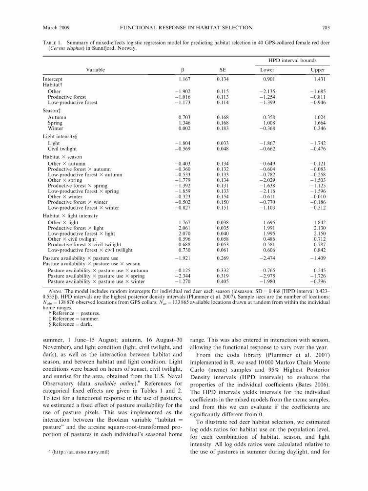
TABLE 1. Summary of mixed-effects logistic regression model for predicting habitat selection in 40 GPS-collared female red deer(Cervus elaphus) in Sunnfjord, Norway.

Variable b SE

HPD interval bounds

Lower Upper

Intercept 1.167 0.134 0.901 1.431Habitat�Other �1.902 0.115 �2.135 �1.685Productive forest �1.016 0.113 �1.254 �0.811Low-productive forest �1.173 0.114 �1.399 �0.946

Season�Autumn 0.703 0.168 0.358 1.024Spring 1.346 0.168 1.008 1.664Winter 0.002 0.183 �0.368 0.346

Light intensity§

Light �1.804 0.033 �1.867 �1.742Civil twilight �0.569 0.048 �0.662 �0.476

Habitat 3 season

Other 3 autumn �0.403 0.134 �0.649 �0.121Productive forest 3 autumn �0.360 0.132 �0.604 �0.083Low-productive forest 3 autumn �0.533 0.133 �0.782 �0.258Other 3 spring �1.779 0.134 �2.029 �1.503Productive forest 3 spring �1.392 0.131 �1.638 �1.125Low-productive forest 3 spring �1.859 0.133 �2.116 �1.596Other 3 winter �0.323 0.154 �0.611 �0.010Productive forest 3 winter �0.502 0.150 �0.770 �0.186Low-productive forest 3 winter �0.827 0.151 �1.103 �0.512

Habitat 3 light intensity

Other 3 light 1.767 0.038 1.695 1.842Productive forest 3 light 2.061 0.035 1.991 2.130Low-productive forest 3 light 2.070 0.040 1.995 2.150Other 3 civil twilight 0.596 0.058 0.486 0.712Productive forest 3 civil twilight 0.688 0.053 0.581 0.787Low-productive forest 3 civil twilight 0.730 0.061 0.606 0.842

Pasture availability 3 pasture use �1.921 0.269 �2.474 �1.409Pasture availability 3 pasture use 3 season

Pasture availability 3 pasture use 3 autumn �0.125 0.332 �0.765 0.545Pasture availability 3 pasture use 3 spring �2.344 0.319 �2.975 �1.726Pasture availability 3 pasture use 3 winter �1.270 0.405 �1.980 �0.396

Notes: The model includes random intercepts for individual red deer each season (idseason; SD ¼ 0.468 [HPD interval 0.423–0.535]). HPD intervals are the highest posterior density intervals (Plummer et al. 2007). Sample sizes are the number of locations:Nobs¼ 138 876 observed locations from GPS collars; Nav¼ 133 865 available locations drawn at random from within the individualhome ranges.

� Reference¼ pastures.� Reference¼ summer.§ Reference¼ dark.

6 hhttp://aa.usno.navy.mili


the average availability of pastures (termed baseline).

Population-level fitted log odds and odds ratios were

calculated as follows. Let x denote a row in the fixed-

effects design matrix, i.e., a vector of covariate values

characterizing a given pixel, and let hj be the ith mcmc

sample from the posterior distribution of the parameter

vector. Then x hj is the ith sample of the fitted log odds

of use for this pixel, for the average individual deer.

Similarly, samples of log odds ratios are calculated as (x

� x0) hj, where x0 characterizes the baseline pixels for

comparison. Interval estimates for fitted odds ratios

were based on 10 000 mcmc samples from the posterior

distribution of the parameters and random effects. The

95% HPD intervals were calculated from the resulting

mcmc samples of fitted values (Bates 2006).

The functional response was visualized by calculating

the population-level log odds ratios of use of pasture

pixels, in the same manner as previously stated, but with

baseline being during darkness and with average

seasonal availability of pastures. Group-level estimates

(i.e., for the ‘‘group’’ of pixels available to an individual

deer) were calculated as follows. Let z denote a row in

the random-effects design matrix (characterizing a

baseline pixel for a specific individual), and let bi be

the ith sample of the random effects. Then x hjþ z bi is

the ith sample of the fitted log odds of use for this pixel

by this individual. Individual-specific odds ratios were

then calculated as (x � x0)hj þ (z � z0)bi, where z0characterizes a baseline pixel (for the same individual)

for comparison. To investigate H2, estimated curves of

constant use were added to the figure. It should be noted

that these curves may be shifted up or down by an

unknown amount, because only relative, not additive,

odds may be estimated with use–availability sampling in

logistic regression. Proportional use would be represent-

ed as horizontal lines (slope ¼ 0).

RESULTS

Temporal scales of habitat selection

The overall selection pattern was quite similar in both

regions (Fig. 2, Tables 1 and 2), indicating that results

are not due to biases introduced by the method used.

Fewer significant variables in Nordfjord most likely

originate from the much lower sample size, as estimates

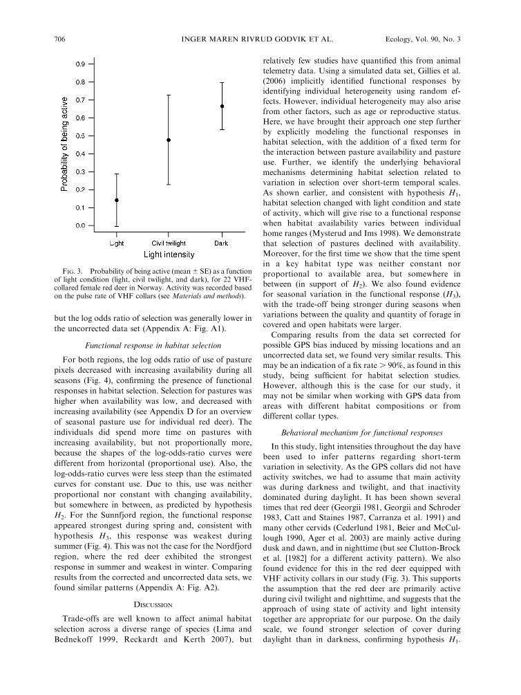
are fairly similar (Table 2). The red deer showed

substantially higher activity levels during darkness than

in daylight, with civil twilight activity levels found in

between (Fig. 3). This also indicates that the activity

sensors in the VHF collars were reliable, as they were

TABLE 2. Summary of the mixed-effects logistic regression model for predicting habitat selection in 22 VHF-collared female reddeer in Nordfjord, Norway.

Variable b SE

HPD interval bounds

Lower Upper

Intercept �1.970 0.566 �3.102 �0.911Habitat�Other �1.818 0.624 �2.982 �0.577Productive forest �1.549 0.575 �2.609 �0.373Low-productive forest �1.420 0.606 �2.559 �0.226

Season�Winter �0.528 0.688 �1.768 0.959

Light intensity§

Light �1.049 0.255 �1.549 �0.563Civil twilight �0.103 0.447 �1.049 0.696

Habitat 3 season

Other 3 winter 0.143 0.717 �1.359 1.478Productive forest 3 winter 0.586 0.692 �0.862 1.870Low-productive forest 3 winter 0.032 0.708 �1.381 1.444

Habitat 3 light intensity

Other 3 light 1.040 0.365 0.378 1.777Productive forest 3 light 1.218 0.271 0.678 1.725Low-productive forest 3 light 1.075 0.333 0.397 1.715Other 3 civil twilight 0.226 0.578 �0.903 1.390Productive forest 3 civil twilight 0.148 0.476 �0.779 1.099Low-productive forest 3 civil twilight 0.104 0.551 �0.952 1.203

Pasture availability 3 pasture use �5.506 2.006 �9.258 �1.567Pasture availability 3 pasture use 3 season

Pasture availability 3 pasture use 3 winter 3.879 2.262 �0.627 8.164

Notes: The model includes random intercepts for individual red deer each season (idseason; SD¼ 2.2310�5 [HPD interval 4.3310�12–1.03 10�7]). HPD intervals are the highest posterior density intervals (Plummer et al. 2007). Nobs¼ 1284 observed locationsfrom GPS collars; Nav ¼ 42 571 available locations drawn at random from within the individual home ranges.

� Reference¼ pastures.� Reference¼ summer.§ Reference ¼ dark.


able to track the expected peaks in activity with

changing light intensity.

The red deer showed a very similar pattern of

selection during all seasons, when separated for the

various light conditions (Fig. 2). As predicted from

hypothesis H1, the main pattern was higher selection for

pastures during darkness, and higher selection for forest

of high productivity during daylight and less during

darkness. During civil twilight, pastures and forest of

high productivity were selected on approximately the

same level. Seasonal differences in selection consisted of

higher selection of pastures in spring and autumn than

in the remaining seasons. During summer, forest of low

productivity was also somewhat more selected.

Comparing the resource selection functions estimated

from the corrected and the uncorrected data set, we

found the overall pattern of selection and relationship

between selection of habitat types to be quite similar,

FIG. 2. Comparing habitat selection through different seasons and light intensities for 62 female red deer in Norway.Estimates are log odds ratios 6 95% highest posterior density intervals, where the log odds ratios are calculated relative toselection of pastures in summer during daylight (reference star). The red line specifies the reference level, and values above 0indicate higher selection of the particular habitat type relative to the reference, whereas values below 0 indicate lower selection.Individuals from Sunnfjord (with GPS collars) are shown in black, and individuals from Nordfjord (with VHF collars) are in blue.The letters P-H-L-O on the x-axis indicate the different habitat types: P, pastures; H, high-productivity forest; L, low-productivityforest; O, other.


but the log odds ratio of selection was generally lower in

the uncorrected data set (Appendix A: Fig. A1).

Functional response in habitat selection

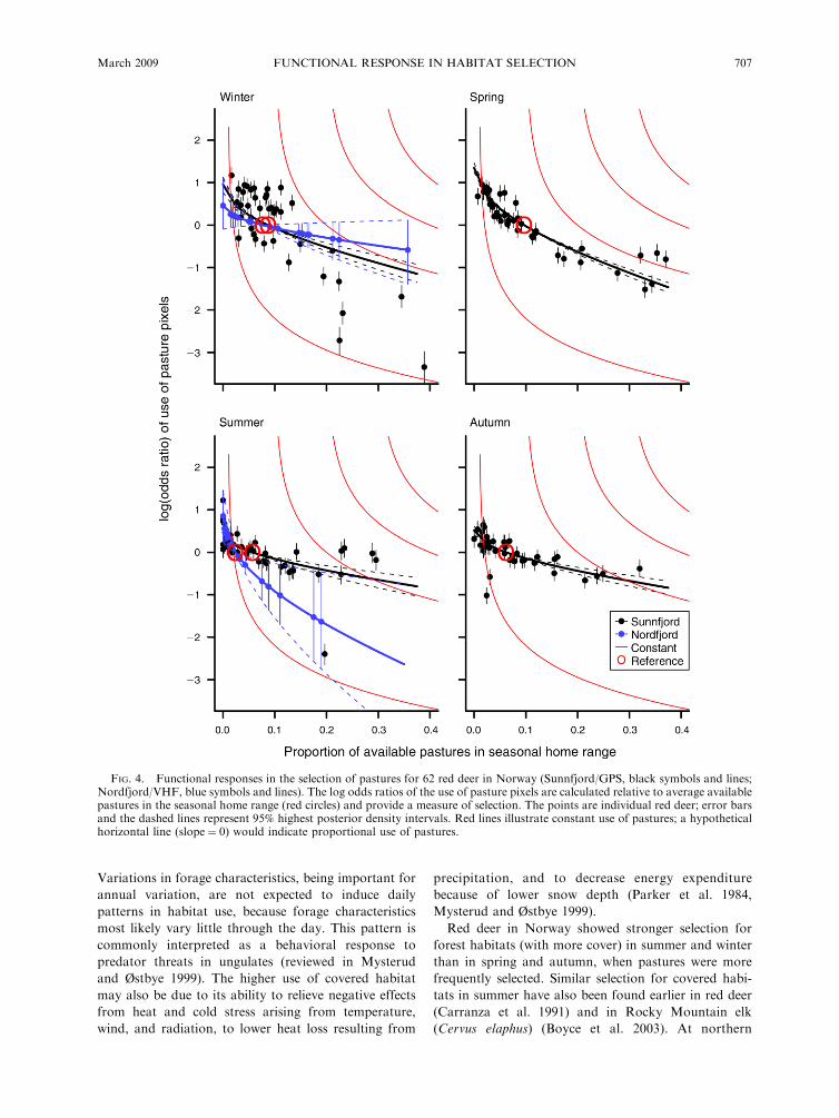
For both regions, the log odds ratio of use of pasture

pixels decreased with increasing availability during all

seasons (Fig. 4), confirming the presence of functional

responses in habitat selection. Selection for pastures was

higher when availability was low, and decreased with

increasing availability (see Appendix D for an overview

of seasonal pasture use for individual red deer). The

individuals did spend more time on pastures with

increasing availability, but not proportionally more,

because the shapes of the log-odds-ratio curves were

different from horizontal (proportional use). Also, the

log-odds-ratio curves were less steep than the estimated

curves for constant use. Due to this, use was neither

proportional nor constant with changing availability,

but somewhere in between, as predicted by hypothesis

H2. For the Sunnfjord region, the functional response

appeared strongest during spring and, consistent with

hypothesis H3, this response was weakest during

summer (Fig. 4). This was not the case for the Nordfjord

region, where the red deer exhibited the strongest

response in summer and weakest in winter. Comparing

results from the corrected and uncorrected data sets, we

found similar patterns (Appendix A: Fig. A2).

DISCUSSION

Trade-offs are well known to affect animal habitat

selection across a diverse range of species (Lima and

Bednekoff 1999, Reckardt and Kerth 2007), but

relatively few studies have quantified this from animal

telemetry data. Using a simulated data set, Gillies et al.

(2006) implicitly identified functional responses by

identifying individual heterogeneity using random ef-

fects. However, individual heterogeneity may also arise

from other factors, such as age or reproductive status.

Here, we have brought their approach one step further

by explicitly modeling the functional responses in

habitat selection, with the addition of a fixed term for

the interaction between pasture availability and pasture

use. Further, we identify the underlying behavioral

mechanisms determining habitat selection related to

variation in selection over short-term temporal scales.

As shown earlier, and consistent with hypothesis H1,

habitat selection changed with light condition and state

of activity, which will give rise to a functional response

when habitat availability varies between individual

home ranges (Mysterud and Ims 1998). We demonstrate

that selection of pastures declined with availability.

Moreover, for the first time we show that the time spent

in a key habitat type was neither constant nor

proportional to available area, but somewhere in

between (in support of H2). We also found evidence

for seasonal variation in the functional response (H3),

with the trade-off being stronger during seasons when

variations between the quality and quantity of forage in

covered and open habitats were larger.

Comparing results from the data set corrected for

possible GPS bias induced by missing locations and an

uncorrected data set, we found very similar results. This

may be an indication of a fix rate . 90%, as found in this

study, being sufficient for habitat selection studies.

However, although this is the case for our study, it

may not be similar when working with GPS data from

areas with different habitat compositions or from

different collar types.

Behavioral mechanism for functional responses

In this study, light intensities throughout the day have

been used to infer patterns regarding short-term

variation in selectivity. As the GPS collars did not have

activity switches, we had to assume that main activity

was during darkness and twilight, and that inactivity

dominated during daylight. It has been shown several

times that red deer (Georgii 1981, Georgii and Schroder

1983, Catt and Staines 1987, Carranza et al. 1991) and

many other cervids (Cederlund 1981, Beier and McCul-

lough 1990, Ager et al. 2003) are mainly active during

dusk and dawn, and in nighttime (but see Clutton-Brock

et al. [1982] for a different activity pattern). We also

found evidence for this in the red deer equipped with

VHF activity collars in our study (Fig. 3). This supports

the assumption that the red deer are primarily active

during civil twilight and nighttime, and suggests that the

approach of using state of activity and light intensity

together are appropriate for our purpose. On the daily

scale, we found stronger selection of cover during

daylight than in darkness, confirming hypothesis H1.

FIG. 3. Probability of being active (mean 6 SE) as a functionof light condition (light, civil twilight, and dark), for 22 VHF-collared female red deer in Norway. Activity was recorded basedon the pulse rate of VHF collars (see Materials and methods).


Variations in forage characteristics, being important for

annual variation, are not expected to induce daily

patterns in habitat use, because forage characteristics

most likely vary little through the day. This pattern is

commonly interpreted as a behavioral response to

predator threats in ungulates (reviewed in Mysterud

and Østbye 1999). The higher use of covered habitat

may also be due to its ability to relieve negative effects

from heat and cold stress arising from temperature,

wind, and radiation, to lower heat loss resulting from

precipitation, and to decrease energy expenditure

because of lower snow depth (Parker et al. 1984,

Mysterud and Østbye 1999).

Red deer in Norway showed stronger selection for

forest habitats (with more cover) in summer and winter

than in spring and autumn, when pastures were more

frequently selected. Similar selection for covered habi-

tats in summer have also been found earlier in red deer

(Carranza et al. 1991) and in Rocky Mountain elk

(Cervus elaphus) (Boyce et al. 2003). At northern

FIG. 4. Functional responses in the selection of pastures for 62 red deer in Norway (Sunnfjord/GPS, black symbols and lines;Nordfjord/VHF, blue symbols and lines). The log odds ratios of the use of pasture pixels are calculated relative to average availablepastures in the seasonal home range (red circles) and provide a measure of selection. The points are individual red deer; error barsand the dashed lines represent 95% highest posterior density intervals. Red lines illustrate constant use of pastures; a hypotheticalhorizontal line (slope¼ 0) would indicate proportional use of pastures.


latitudes, there is strong seasonal variation in forage

quality and quantity (Clutton-Brock et al. 1982, Albon

and Langvatn 1992, Van Soest 1994), and to some extent

also in canopy cover in the different habitats (Mysterud

and Østbye 1999). Pastures, in our study area mainly

meadows with timothy, hold forage of higher quality

and abundance relative to forested habitats throughout

the year (Albon and Langvatn 1992). However, snow

cover leads to increased energy expenditures for

movement and inhibits access to forage (Parker et al.

1984). Several studies on ungulates have reported

increased use of older forest when snow depth was

greater (Armleder et al. 1994, Poole and Mowat 2005,

Jenkins et al. 2007), which probably explains the

lowered selection of pastures during winter in our study.

In summer, although not well quantified, the quality and

quantity of forage in the forested areas probably

approach those of pastures in summer due to higher

productivity, which together with mothers having

offspring (at a higher risk of being predated) can explain

the higher selection of covered areas during summer.

Calves exhibit reduced mobility during this period, and

staying in covered habitats could lower the risk of

predation on the calves.

Variations in the strength of trade-offs

The red deer in this study exhibited a functional

response in selection of pastures, as predicted by

hypothesis H2. This was apparent through all seasons,

indicating that they experienced trade-offs involving

activities that are spatially segregated and specific to the

various habitats. The strength of the trade-off and the

functional response varied with both habitat availability

and seasons. The time spent on pastures increased with

increasing availability, but not in a directly proportional

manner, leading to the strength of the trade-off varying

with habitat availability driven by landscape-level

variability. The seasonal variation in the trade-off may

be due to seasonally varying abundance of forage and

cover in the different habitats. In autumn and spring,

selection of open and covered habitats differed consid-

erably through the day, as adequate cover and highly

nutritious forage are rarely found in the same habitat. In

contrast, the shifting of habitats through the day was

less pronounced during summer and winter. In summer,

vegetation is generally abundant in forests as well, while

during winter snow cover may prevent the red deer from

utilizing pastures to a large extent. The functional

response was less apparent in summer than in the

remaining seasons; during spring the functional response

was strongest. This is probably a consequence of the

different distribution of forage and cover through the

seasons. However, the seasonal pattern in the functional

response differed in the two regions. In contrast to

Sunnfjord, the functional response was strongest in

summer and weakest during winter in the Nordfjord

region. Within home ranges in Nordfjord, there was

15.5% more forest of high productivity than in

Sunnfjord, and 12% less marshland and mountains,

whereas the distribution of the other habitat types was

approximately equal. Thus, we may speculate that an

interaction between seasonality and landscape architec-

ture could be affecting these trade-offs.

In elk, highly nutritious forage on meadows was

traded for lower quality forage in forests during the

hunting season (Morgantini and Hudson 1985). Wheth-

er individuals taking a higher risk as the availability of

pastures increases in the landscape actually grow more,

at the risk of being predated, remains to be determined.

Indeed, relating multiple-habitat-type use to fitness traits

is possible and clearly a goal, but obtaining such data is

extremely difficult and has so far only been done for the

island population on Rum, Scotland (McLoughlin et al.

2006).

Concluding remarks

In many areas of the western world, deer populations

have been expanding and increasing greatly in density in

recent decades, causing concern regarding damage to

agricultural crops, forestry, and biodiversity in their

natural habitats (McShea et al. 1997, Gordon et al.

2004). The strong shifts in trade-offs linked to habitat

selection shown here, driven by landscape-level variation

in habitat compositions, will change the spatial distri-

bution of grazing pressure, and therefore the resulting

pressure on pastures relative to their natural habitat.

Our study, in addition to yielding novel insight into deer

behavior, thus also has the potential to enable more

accurate predictions of damage to agricultural crops and

threat to biodiversity as a function of landscape.

ACKNOWLEDGMENTS

This research was funded by the Research Council ofNorway (AREAL-program and YFF-grant to A. Mysterud)and the Directorate for Nature Management. We are grateful toKnut Førde, Harald Kjær, and Odd Rønningen for help duringfieldwork, and to Michael Angeloff for DEM-maps. We aregrateful for helpful comments from Mark Hewison and AlainLicoppe on a previous draft.

LITERATURE CITED

Abrahamsen, J., N. K. Jacobsen, R. Kalliola, E. Dahl, L.Wilborg, and L. Pahlson. 1977. Naturgeografisk regioninndel-ing av Norden. Nordiske Utredninger Series B 34:1–135.

Ager, A. A., B. K. Johnson, J. W. Kern, and J. G. Kie. 2003.Daily and seasonal movements and habitat use by femaleRocky Mountain elk and mule deer. Journal of Mammalogy84:1076–1088.

Albon, S. D., and R. Langvatn. 1992. Plant phenology and thebenefits of migration in a temperate ungulate. Oikos 65:502–513.

Armleder, H. M., M. J. Waterhouse, D. G. Keisker, and R. J.Dawson. 1994. Winter habitat use by mule deer in the centralinterior of British Colombia. Canadian Journal of Zoology72:1721–1725.

Armstrong, E., D. Euler, and G. Racey. 1983. White-tailed deerhabitat and cottage development in central Ontario. Journalof Wildlife Management 47:605–612.

Bates, D. M. 2006. lmer, P-values and all that. hhttps://stat.ethz.ch/pipermail/r-help/2006-May/094765.htmli


Bates, D. M. 2007. lme4: Linear mixed-effects models using S4classes. R package version 0.99875-9.

Beier, P., and D. R. McCullough. 1988. Motion-sensitive radiocollars for estimating white-tailed deer activity. Journal ofWildlife Management 52:11–13.

Beier, P., and D. R. McCullough. 1990. Factors influencingwhite-tailed deer activity patterns and habitat use. WildlifeMonographs 109:5–51.

Boyce, M. S., J. S. Mao, E. H. Merrill, D. Fortin, M. G.Turner, J. Fryxell, and P. Turchin. 2003. Scale andheterogeneity in habitat selection by elk in YellowstoneNational Park. Ecoscience 10:421–431.

Boyce, M. S., P. R. Vernier, S. E. Nielsen, and F. K. A.Schmiegelow. 2002. Evaluating resource selection functions.Ecological Modelling 157:281–300.

Carranza, J., S. J. H. Detrucios, R. Medina, J. Valencia, and J.Delgado. 1991. Space use by red deer in a Mediterraneanecosystem as determined by radio-tracking. Applied AnimalBehaviour Science 30:363–371.

Catt, D. C., and B. W. Staines. 1987. Home range use andhabitat selection by red deer (Cervus elaphus) in a Sitkaspruce plantation as determined by radio-tracking. Journal ofZoology 211:681–693.

Cederlund, G. 1981. Daily and seasonal activity pattern of roedeer in a boreal habitat. Viltrevy 11:315–353.

Clutton-Brock, T. H., F. E. Guinness, and S. D. Albon. 1982.Red deer: behavior and ecology of the two sexes. Universityof Chicago Press, Chicago, Illinois, USA.

D’Eon, R. G. 2003. Effects of a stationary GPS fix-rate bias onhabitat selection analyses. Journal of Wildlife Management67:858–863.

D’Eon, R. G., and D. Delparte. 2005. Effects of radio-collarposition and orientation on GPS radio-collar performance,and the implications of PDOP in data screening. Journal ofApplied Ecology 42:383–388.

D’Eon, R. G., R. Serrouya, G. Smith, and C. O. Kochanny.2002. GPS radiotelemetry error and bias in mountainousterrain. Wildlife Society Bulletin 30:430–439.

ESRI. 2006. ArcMAP 9.2. ESRI (Environmental SystemsResearch Institute). Redlands, California, USA.

Frair, J. L., S. E. Nielsen, E. H. Merrill, S. R. Lele, M. S.Boyce, R. H. M. Munro, G. B. Stenhouse, and H. L. Beyer.2004. Removing GPS collar bias in habitat selection studies.Journal of Applied Ecology 41:201–212.

Georgii, B. 1981. Activity patterns of female red deer (Cervuselaphus L.) in the Alps. Oecologia 49:127–136.

Georgii, B., and W. Schroder. 1983. Home range and activitypatterns of male red deer (Cervus elaphus L.) in the Alps.Oecologia 58:238–248.

Gillies, C. S., M. Hebblewhite, S. E. Nielsen, M. A. Krawchuk,C. L. Aldridge, J. L. Frair, D. J. Saher, C. E. Stevens, andC. L. Jerde. 2006. Application of random effects to the studyof resource selection by animals. Journal of Animal Ecology75:887–898.

Gillingham, M. P., K. L. Parker, and T. A. Hanley. 1997.Forage intake by black-tailed deer in a natural environment:bout dynamics. Canadian Journal of Zoology 75:1118–1128.

Gordon, I. J., A. J. Hester, and M. Festa-Bianchet. 2004. Themanagement of wild large herbivores to meet economic,conservation and environmental objectives. Journal ofApplied Ecology 41:1021–1031.

Graves, T. A., and J. S. Waller. 2006. Understanding the causesof missed global positioning system telemetry fixes. Journalof Wildlife Management 70:844–851.

Hansen, M. C., G. W. Garner, and S. G. Fancy. 1992.Comparison of 3 methods for evaluating activity of Dallsheep. Journal of Wildlife Management 56:661–668.

Hebblewhite, M., and E. Merrill. 2008. Modeling wildlife–human relationships for social species with mixed-effectsresource selection models. Journal of Applied Ecology 45:834–844.

Jenkins, D. A., J. A. Schaefer, R. Rosatte, T. Bellhouse, J.Hamr, and F. F. Mallory. 2007. Winter resource selection ofreintroduced elk and sympatric white-tailed deer at multiplespatial scales. Journal of Mammalogy 88:614–624.

Johnson, B. K., J. W. Kern, M. J. Wisdom, S. L. Findholt, andJ. G. Kie. 2000. Resource selection and spatial separation ofmule deer and elk during spring. Journal of WildlifeManagement 64:685–697.

Johnson, D. H. 1980. The comparison of usage and availabilitymeasurements for evaluating resource preference. Ecology61:65–71.

Langvatn, R., S. D. Albon, T. Burkey, and T. H. Clutton-Brock. 1996. Climate, plant phenology and variation in ageof first reproduction in a temperate herbivore. Journal ofAnimal Ecology 65:653–670.

Lemaitre, J., and M. A. Villard. 2005. Foraging patterns ofpileated woodpeckers in a managed Acadian forest: aresource selection function. Canadian Journal of ForestResearch 35:2387–2393.

Lima, S. L., and P. A. Bednekoff. 1999. Temporal variation indanger drives antipredator behavior: The predation riskallocation hypothesis. American Naturalist 153:649–659.

Lima, S. L., and L. M. Dill. 1990. Behavioral decisions madeunder the risk of predation: a review and prospectus.Canadian Journal of Zoology 68:619–640.

Manly, B. F. J., L. L. McDonald, D. L. Thomas, T. L.McDonald, and W. P. Erickson. 2002. Resource selection byanimals: statistical design and analysis for field studies.Second edition. Kluwer Academic Publishers, Dordrecht,The Netherlands.

Mauritzen, M., S. E. Belikov, A. N. Boltunov, A. E. Derocher,E. Hansen, R. A. Ims, O. Wiig, and N. Yoccoz. 2003.Functional responses in polar bear habitat selection. Oikos100:112–124.

McLoughlin, P. D., M. S. Boyce, T. Coulson, and T. Clutton-Brock. 2006. Lifetime reproductive success and density-dependent, multi-variable resource selection. Proceedings ofthe Royal Society B 273:1449–1454.

McShea, M. J., H. B. Underwood, and J. H. Rappole. 1997.The science of overabundance: deer ecology and populationmanagement. Smithsonian Institution Press, Washington,D.C., USA.

Morgantini, L. E., and R. J. Hudson. 1985. Changes in diets ofwapiti during a hunting season. Journal of Range Manage-ment 38:77–79.

Morris, D. W. 1987. Ecological scale and habitat use. Ecology68:362–369.

Mysterud, A., and R. A. Ims. 1998. Functional responses inhabitat use: availability influences relative use in trade-offsituations. Ecology 79:1435–1441.

Mysterud, A., P. K. Larsen, R. A. Ims, and E. Ostbye. 1999.Habitat selection by roe deer and sheep: does habitat rankingreflect resource availability? Canadian Journal of Zoology 77:776–783.

Mysterud, A., and E. Østbye. 1999. Cover as a habitat elementfor temperate ungulates: effects on habitat selection anddemography. Wildlife Society Bulletin 27:385–394.

Mysterud, A., N. G. Yoccoz, N. C. Stenseth, and R. Langvatn.2000. Relationships between sex ratio, climate and density inred deer: the importance of spatial scale. Journal of AnimalEcology 69:959–974.

Nielsen, S. E., M. S. Boyce, G. B. Stenhouse, and R. H. M.Munro. 2002. Modeling grizzly bear habitats in the Yellow-head ecosystem of Alberta: taking autocorrelation seriously.Ursus 13:45–56.

Orians, G. H., and J. F. Wittenberger. 1991. Spatial andtemporal scales in habitat selection. American Naturalist 137:S29–S49.

Osko, T. J., M. N. Hiltz, R. J. Hudson, and S. M. Wasel. 2004.Moose habitat preferences in response to changing availabil-ity. Journal of Wildlife Management 68:576–584.


Parker, K. L., C. T. Robbins, and T. A. Hanley. 1984. Energyexpenditures for locomotion by mule deer and elk. Journal ofWildlife Management 48:474–488.

Plummer, M., N. Best, K. Cowles, and K. Vines. 2007. CODA:output analysis and diagnostics for MCMC. R packageversion 0.12-1. hhttp://www.r-project.org/i

Poole, K. G., and G. Mowat. 2005. Winter habitat relationshipsof deer and elk in the temperate interior mountains of BritishColumbia. Wildlife Society Bulletin 33:1288–1302.

R Development Core Team. 2008. R: A language andenvironment for statistical computing. R Foundation forStatistical Computing, Vienna, Austria.

Reckardt, K., and G. Kerth. 2007. Roost selection and roostswitching of female Bechstein’s bats (Myotis bechsteinii) as astrategy of parasite avoidance. Oecologia 154:581–588.

Rosenzweig, M. L. 1981. A theory of habitat selection. Ecology62:327–335.

Senft, R. L., M. B. Coughenour, D. W. Bailey, L. R.Rittenhouse, O. E. Sala, and D. M. Swift. 1987. Large

herbivore foraging and ecological hierarchies. BioScience 37:789–799.

Sih, A. 1980. Optimal foraging: Can foragers balance twoconflicting demands? Science 210:1041–1043.

Skrondal, A., and S. Rabe-Hesketh. 2004. Generalized latentvariable modeling: multilevel, longitudinal, and structuralequation models. Chapman and Hall, New York, New York,USA.

Van Soest, P. J. 1994. Nutritional ecology of the ruminant.Second edition. Cornell University Press, New York, NewYork, USA.

Werner, E. E., J. F. Gilliam, D. J. Hall, and G. G. Mittelbach.1983. An experimental test of the effects of predation risk onhabitat use in fish. Ecology 64:1540–1548.

White, G. C., and R. A. Garrott. 1990. Analysis of wildliferadio-tracking data. Academic Press, London, UK.

Wood, S. N. 2006. Generalized additive models: an introduc-tion with R. Chapman and Hall/CRC, Boca Raton, Florida,USA.

APPENDIX A

A detailed description of how GPS bias was corrected for and the minor effect this had on the results (Ecological Archives E090-049-A1).

APPENDIX B

Error ellipses for VHF data (Ecological Archives E090-049-A2).

APPENDIX C

Habitat classifications from digital resource maps provided by the Norwegian Forest and Landscape Institute (EcologicalArchives E090-049-A3).

APPENDIX D

Plots showing use of pastures for 62 female red deer in Norway in relation to availability (Ecological Archives E090-049-A4).


temporal scales, trade-offs, and functional responses in red deer habitat selection

Documents