temperature trends in the lower atmosphere: steps … · temperature trends in the lower atmosphere...

Temperature Trends in the Lower Atmosphere - Understanding and Reconciling Differences

Why do temperatures vary vertically (from the surface to the stratosphere) and what do we understand about why they might vary and change over time?

Convening Lead Author: V. Ramaswamy, NOAALead Authors: J.W. Hurrell, NSF NCAR; G.A. Meehl, NSF NCARContributing Authors: A. Phillips, NCAR, Boulder; B.D. Santer, DOE LLNL; M.D. Schwarzkopf, NOAA; D.J. Seidel, NOAA; S.C. Sherwood, Yale Univ.; P.W. Thorne, U.K. Met. OfficeC

HA

PTER

1

PB 15

Temperature trends at the surface

can be expected to be different

from temperature trends higher in the

atmosphere.

SUMMARy

Temperatures Vary VerticallyThe global temperature profile of the Earth’s atmosphere reflects a balance between the radia-tive, convective and dynamical heating/cooling of the surface-atmosphere system. Radiation from the Sun is the source of energy for the Earth’s climate, with most of it absorbed at the surface. Combined with the physical properties of the atmosphere and dynamical processes, the heat is mixed vertically and horizontally, yielding the highest temperatures, on average, at the surface, with marked seasonal and spatial variations. In the atmosphere, the distribution of moisture and the lower air pressure at progressively higher altitudes result in decreasing temperatures with height up to the tropopause, with the rate of decrease depending on geographical factors and meteorological conditions. The tropopause marks the top of the troposphere, i.e., the lower 8 to 16 km of the atmosphere (see Preface, Fig. 2), and varies with latitude and longitude. Above this altitude, the physical properties of the air produce a warming with height through the stratosphere (extending from the tropopause to ~50 km).

Temperature trends at the surface can be expected to be different from temperature trends higher in the atmosphere because:• Surface types (sea, snow, ice, and different vegetative covers of land) differ considerably in

their physical properties. Near the surface, these differing conditions can produce strong horizontal variations in temperature. Above the surface layer, these contrasts are quickly smoothed out by the atmospheric motions, contributing to varying temperature trends with height at different locations.

• Changes in atmospheric circulation or modes of atmospheric variability (e.g., El Niño-Southern Oscillation [ENSO]) can produce different temperature trends at the surface and aloft.

• Under some circumstances, temperatures may increase with height near the surface or higher in the troposphere, producing a "temperature inversion." Such inversions are more common at night; over continents, sea ice and snow during winter; and in the trade wind regions. Since the air in inversion layers is resistant to vertical mixing, temperatures trends can differ between inversion layers and adjacent layers.

• Forcing factors, either natural (e.g., volcanoes and solar) or human-induced (e.g., greenhouse gas, aerosols, ozone, and land use) can result in differing temperature trends at different altitudes, and these vertical variations may change over time. This can arise due to spatial and temporal changes in the concentrations or properties of the forcing agents.

The U.S. Climate Change Science Program Chapter 1

16 1716 17

This Chapter describes the temperature profile of the layers of the atmosphere from the surface through the stratosphere and discusses the basic reasons for this profile. We also use results from global climate model simulations to show how changes in natural and human-induced fac-tors can produce different temperature trends in the various layers of the atmosphere. This discussion provides the background for the presentation of the observed changes (Chapters 2-4), and for the understanding of their causes (Chapter 5). We also describe temperature changes in the stratosphere in recent decades and the influences of these changes on the troposphere. Finally, making use of surface and satellite observations, we examine the physical processes that can result in different temperature trends at the surface and in the troposphere.

1.1 THE THERMAL STRUCTURE oF THE ATMoSPHERE

Radiation input from the Sun is the source of en-ergy for the Earth’s climate system (Hartmann, 1994). Most of the solar radiation absorbed is at the surface, the rest being absorbed by the atmosphere. The global-and-annual-mean so-lar radiation absorbed and outgoing longwave emission from Earth balance each other to yield a steady-state climate for the planet as a whole. Both radiation components have a maximum in the tropics and decrease towards the poles. There is an excess of net radiative (solar+longwave) heating of the climate system in the tropics, with a deficit in the high latitudes (poleward of ~400). Dynamical motions aris-ing as a consequence of this equator-to-pole gradient, combined with convective processes and the influence due to the rotation of the Earth, result in a heat transfer from the low to middle and high latitudes, thereby setting up the climatological horizontal and vertical thermal structure (Hartmann, 1994; Salby, 1996).

Surface temperatures are at their warmest in the tropics, where the largest amount of solar radia-tion is received during the course of the year, and decrease towards the polar regions where the annual-mean solar radiation received is at a minimum (Oort and Peixoto, 1992). The tem-perature contrast between summer and winter is greatest at the poles and least at the Equator. Since land areas heat up and cool more rapidly than oceans, and because of the preponderance of land in the Northern Hemisphere, there is a larger contrast in temperature between summer and winter in the Northern Hemisphere.

Figure 1.1 illustrates the climatological vertical temperature profiles for December, January, February and June, July, August mean condi-tions, as obtained from the National Centers for Environmental Prediction (NCEP) reanalyses (Kalnay et al., 1996; updated). It is convenient to think first in terms of climatological conditions upon which spatial and temporal variations/trends are superimposed. The solid line in the plot estimates the tropopause, which separates the troposphere below from the stratosphere above (see Preface, Fig. 2). The tropopause is at its highest level in the tropics (~20°N-20°S). It descends sharply in altitude from ~16 km at the equator to ~12 km at ~30-40° latitude, and to as low as about 9 km at the poles.

Temperatures generally decrease with height from the surface although there are important exceptions. The rate at which the temperature changes with height is termed the “lapse rate.” The lapse rate can vary with location and sea-son, and its value depends strongly on the atmo-spheric humidity, e.g., the lapse rate varies from ~4ºC/km near the surface in the moist tropical regions (near the equator) to much larger values (~8-9ºC/km) in the drier subtropics (~20-30°). Important departures from nominal lapse rate values can occur near the surface and in the upper troposphere. In the equatorial tropics, the tropopause region (~16 km) is marked by a smaller value of the lapse rate than in the lower troposphere.

The thermal structure of the lowest 2-3 km, known as the “planetary boundary layer,” can be complicated, even involving inver-

The rate at which the temperature changes with height is termed the “lapse rate.” The lapse rate can vary with location and season, and its value depends strongly on the atmospheric humidity.

16 17


16 17

sions (in which temperature increases rather than decreases with height) occurring at some latitudes due to land-sea contrasts, topographic influences, radiative effects and meteorological conditions. Inversions are particularly com-mon during winter over some middle and high latitude land regions and are a climatological feature in the tropical trade wind regions. The presence of inversions acts to decouple surface

temperatures from tropospheric temperatures on daily or even weekly timescales.

Above the tropopause is the stratosphere, which extends to ~50 km and in which the tempera-ture increases with height. In the vicinity of the tropical tropopause, (i.e., the upper tropo-sphere and lower stratosphere regions, ~15-18 km), the temperature varies little with height.

The extratropical (poleward of 30°) lower stratosphere (at ~8-12 km) also exhibits a similar feature (Holton, 1979). The lapse rate change with altitude in the upper tro-posphere/lower stratosphere region is less sharp in the extratropical latitudes than in the tropics.

The global temperature pro-file of the atmosphere reflects a balance between the radia-tive, convective and dynami-cal heating/cooling of the surface-atmosphere system. From a global, annual-aver-age point of view, the thermal profile of the stratosphere is the consequence of a balance between radiative heating and cooling rates due to green-house gases, principally car-bon dioxide (CO2), ozone (O3) and water vapor (H2O) (An-drews et al., 1987). The verti-cal profile in the troposphere is the result of a balance of radiative processes involving greenhouse gases, aerosols, and clouds (Stephens and Webster, 1981; Goody and Yung, 1989), along with the strong role of moist convec-tion and dynamical motions (Holton, 1979; Held, 1982; Kiehl, 1992). An important difference between the tro-posphere and stratosphere is that the stratosphere is characterized by weak ver-tical motions, while in the troposphere, the vertical mo-

The presence of inversions acts to decouple surface

temperatures from tropospheric

temperatures on daily or even

weekly timescales.

Figure 1.1. Global climatological vertical temperature profiles from surface to troposphere and extending into the stratosphere for December-January-February (DJF) and June-July-August (JJA) mean conditions (1979-2003), as obtained from the National Centers for Environmental Prediction (NCEP) reanalyses (Kalnay et al., 1996; updated). The solid line denotes the tropopause which separates the stratosphere from the surface-troposphere system. The tropopause pressure level is defined by the standard lapse rate criterion: it is identified by the lowest level (above 450 hPa) where the temperature lapse rate becomes less than 2ºC/km. The tropopause pressure archived in the reanalyses is estimated by deriving the lapse rate at each model level and estimating (by interpolation in height) the pressure where the threshold value of 2ºC/km is reached. This algorithm produces tropopause estimates which vary smoothly in space and time.


18 1918 19

tions are stronger. Most significantly, the moist convective processes that are a characteristic feature of the troposphere include the transfer of large amounts of heat due to evaporation or condensation of water.

A useful conceptual picture of the thermal structure can be had by considering the radia-tive-convective balance that is approximately applicable to the tropics taken as a whole. If radiative processes alone were considered, that would cause the surface to be significantly warmer than it is actually (Goody and Yung, 1989). This would occur because the atmo-sphere is relatively transparent to the Sun’s radiation. This would lead to a strong heating of the surface accompanied by a net radiative cooling of the atmosphere (Manabe and Weth-erald, 1967). However, the resulting convective motions remove the excess heating from the surface in the form of sensible and latent heat, the latter involving the evaporation of moisture from the surface (Ramanathan and Coakley, 1978). As air parcels rise and expand, they cool due to decompression, leading to a decrease of temperature with height. The lapse rate for a dry atmosphere, when there are no moist pro-cesses and the air is rising quickly enough to be unaffected by other heating/cooling sources, is close to 10ºC/km. However, because of moist convection, there is condensation of moisture, formation of clouds and release of latent heat as the air parcels rise, causing the lapse-rate to be much less, as low as 4ºC/km in very humid atmospheres (Houghton, 1977).

Actual thermal profiles are more complex than above owing to the additional roles of the large-scale circulation and convection-cloud physical interactions. For example, a more de-tailed picture in subtropical regions consists of a surface mixed layer (up to about 500 m) and a trade wind boundary layer (up to about 2 km) above which is the free troposphere. Each of the boundary layers is topped by an inversion which tends to isolate the region from the layer above (Sarachik, 1985). This indicates the limitations in assuming nominal lapse rate values from the surface to the tropopause everywhere. In the tropical upper troposphere, moisture- and cloud-related features related to convection (e.g., upper tropospheric relative humidity, cirrus cloud microphysics, and mesoscale cir-

culations in anvil clouds) are important factors in shaping the thermal profile (Ramaswamy and Ramanathan, 1989; Donner et al., 2001; Sherwood and Dessler, 2003). In the more general sense, the interactions be-tween radiation, moist convection, and dynami-cal motions (ranging from large- to meso- and small-scales) govern the quantitative rate at which temperature decreases with height at any location. Large-scale dynamical mechanisms tend to result in more spatially uniform tem-peratures (on monthly-mean and longer time scales) above the boundary layer, and over hori-zontal scales (Rossby radius; Hartmann, 1994) that vary from planetary scale near the equator to a couple of thousand kilometers at middle latitudes and to a few hundred kilometers near the poles. The major circulation patterns in the atmosphere such as the Hadley and Walker cir-culations (Holton, 1979; Hartmann, 1994) play a key role in the atmospheric energy balance of the tropics and subtropics (~30 degrees in latitude), and this crucially affects the thermal structure in those regions (Trenberth and Stepa-niak, 2003). The low latitudes are characterized by a vertical coherence in the vertical tempera-ture structure, with variations of opposite signs in temperature below and above the tropopause associated with upward motion and subsidence, respectively (Trenberth and Smith, 2006). In the extra-tropics (poleward of 30° latitude), the lapse rate and tropopause height are affected by instabilities associated with large-scale eddies of the familiar weather systems (“baroclinic instability”; Holton, 1979; Held, 1982). In the polar regions (~60-90°), planetary-scale waves forced by the influences of mountains and that of land-sea contrasts upon the flow of air play a significant role in the determination of the wintertime temperatures at the poles. The sense of the radiative-convective-dynami-cal balance above, together with the require-ment of radiative balance at the top-of-the-atmosphere (namely, equilibrium conditions wherein the net solar energy absorbed by the Earth’s climate system must be balanced by the infrared radiation emitted by the Earth), can help illustrate the significance of long-lived infrared absorbing gases in the global atmosphere. The presence of such greenhouse gases (e.g., carbon dioxide, methane, nitrous

As air parcels rise and expand, they cool due to decompression, leading to a decrease of temperature with height.

18 19


18 19

oxide, halocarbons) increases the radiative heat-ing of the surface and troposphere. As specific humidity is strongly related to temperature, it is expected to rise with surface warming (IPCC, 1990), The increased moisture content of the atmosphere amplifies the initial radiative heating due to the greenhouse gas increases (Manabe and Wetherald, 1967; Ramanathan, 1981). The re-establishment of a new thermal equilibrium in the climate system involves the communication of the added heat input to the troposphere and surface, leading to surface warming (Goody and Yung, 1989; IPCC, 1990; Lindzen and Emanuel, 2002). From the preceding discussions, the lapse rate can be expected to decrease with the resultant increase in humidity, and also to depend on the resultant changes in atmospheric circulation. In general, the lapse rate can be expected to decrease with warming such that temperature changes aloft exceed those at the surface. As a consequence, the characteristic infrared emission level of the planet is shifted to a higher altitude in the atmosphere.

1.2 nATURAL And AnTHRoPoGEn�C FoRC�nG oF CL�MATE CHAnGE

Potentially significant variations and trends are superimposed on the basic climatological thermal profile, as revealed by observational data in the subsequent chapters. While the knowledge of the climatological mean structure discussed in the previous section involves considerations of radiative, convective, and dynamical processes, understanding the features and causes of the magnitude of changes involves a study of the perturbations in these processes, which then frame the response of the climate system to the forcing. While the understanding of climate variability is primarily based on observations of substantial changes (e.g., sea-surface temperature changes during El Niño), the vertical temperature changes being investigated in this report are changes on the order of a few tenths of degrees on the global-mean scale (local changes could be much greater), as discussed in the subsequent chapters.

“Unforced” variations, i.e., changes arising from internally generated variations in the at-mosphere-ocean-land-ice/snow climate system, can influence surface and atmospheric tem-peratures substantially, e.g., due to changes in equatorial sea-surface temperatures associated with ENSO. Climate models indicate that glob-al-mean unforced variations on multidecadal timescales are likely to be smaller than, say, the 20th century global-mean increase in surface temperature (Stouffer et al., 2000). However, for specific regions and/or seasons, this may not be valid and the unforced variability could be substantial. Chapter 5 provides more detail on models and their limitations (see particularly Box 5.1 and 5.2).

Because of the influence of radiative processes on the thermal structure, any agent external to the climate system that perturbs the planet’s radiative heating distribution can cause climate changes, and thus is potentially important in ac-counting for the observed temperature changes (Santer et al., 1996). The radiative (solar plus longwave) heat balance of the planet can be perturbed (forced) by:

• natural factors such as changes in the Sun’s irradiance, and episodic, explosive volcanic events (leading to a build-up of particulates in the stratosphere);

• human-induced factors such as changes in the concentrations of radiatively active gases (carbon dioxide, methane, etc.) and aerosols.

Important external forcing agents of relevance for the surface and atmospheric temperature changes since pre-industrial time (1750) are summarized in Table 1.1. As illustrative ex-amples, global-mean forcing estimates for the period 1750 to ~2000 (late 1990s) are listed. For more details, see Ramaswamy et al. (2001) and NRC (2005).

From Table 1.1, the important anthropogenic contributions to the global-mean forcing since pre-industrial times to ~2000 are due to well-mixed greenhouse gases and ozone, aerosols, and land-use (albedo). The natural factors are comprised of solar irradiance variations and stratospheric aerosols in the aftermath of explo-

The lapse rate can be expected to decrease

with warming such that temperature

changes aloft exceed those at the surface.


20 2120 21

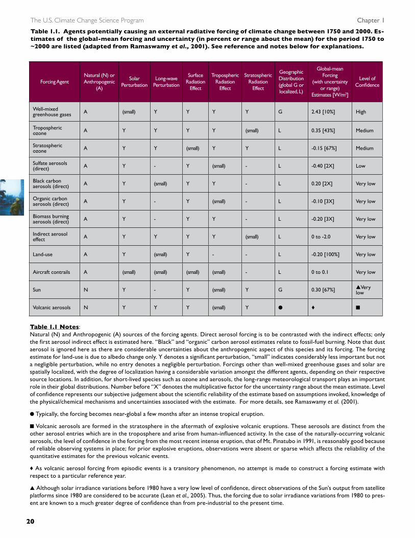
Table 1.1. Agents potentially causing an external radiative forcing of climate change between 1750 and 2000. Es-timates of the global-mean forcing and uncertainty (in percent or range about the mean) for the period 1750 to ~2000 are listed (adapted from Ramaswamy et al., 2001). See reference and notes below for explanations.

Forcing AgentNatural (N) or Anthropogenic

(A)

Solar Perturbation

Long-wave Perturbation

Surface Radiation

Effect

Tropospheric Radiation

Effect

Stratospheric Radiation

Effect

Geographic Distribution (global G or localized, L)

Global-mean Forcing

(with uncertainty or range)

Estimates [W/m2]

Level of Confidence

Well-mixed greenhouse gases A (small) Y Y Y Y G 2.43 [10%] High

Tropospheric ozone A Y Y Y Y (small) L 0.35 [43%] Medium

Stratospheric ozone A Y Y (small) Y Y L -0.15 [67%] Medium

Sulfate aerosols (direct) A Y - Y (small) - L -0.40 [2X] Low

Black carbon aerosols (direct) A Y (small) Y Y - L 0.20 [2X] Very low

Organic carbon aerosols (direct) A Y - Y (small) - L -0.10 [3X] Very low

Biomass burning aerosols (direct) A Y - Y Y - L -0.20 [3X] Very low

Indirect aerosol effect A Y Y Y Y (small) L 0 to -2.0 Very low

Land-use A Y (small) Y - - L -0.20 [100%] Very low

Aircraft contrails A (small) (small) (small) (small) - L 0 to 0.1 Very low

Sun N Y - Y (small) Y G 0.30 [67%] ▲Very low

Volcanic aerosols N Y Y Y (small) Y ● ♦ ■

Table 1.1 notes: Natural (N) and Anthropogenic (A) sources of the forcing agents. Direct aerosol forcing is to be contrasted with the indirect effects; only the first aerosol indirect effect is estimated here. “Black” and “organic” carbon aerosol estimates relate to fossil-fuel burning. Note that dust aerosol is ignored here as there are considerable uncertainties about the anthropogenic aspect of this species and its forcing. The forcing estimate for land-use is due to albedo change only. Y denotes a significant perturbation, “small” indicates considerably less important but not a negligible perturbation, while no entry denotes a negligible perturbation. Forcings other than well-mixed greenhouse gases and solar are spatially localized, with the degree of localization having a considerable variation amongst the different agents, depending on their respective source locations. In addition, for short-lived species such as ozone and aerosols, the long-range meteorological transport plays an important role in their global distributions. Number before “X” denotes the multiplicative factor for the uncertainty range about the mean estimate. Level of confidence represents our subjective judgement about the scientific reliability of the estimate based on assumptions invoked, knowledge of the physical/chemical mechanisms and uncertainties associated with the estimate. For more details, see Ramaswamy et al. (2001).

● Typically, the forcing becomes near-global a few months after an intense tropical eruption.

■ Volcanic aerosols are formed in the stratosphere in the aftermath of explosive volcanic eruptions. These aerosols are distinct from the other aerosol entries which are in the troposphere and arise from human-influenced activity. In the case of the naturally-occurring volcanic aerosols, the level of confidence in the forcing from the most recent intense eruption, that of Mt. Pinatubo in 1991, is reasonably good because of reliable observing systems in place; for prior explosive eruptions, observations were absent or sparse which affects the reliability of the quantitative estimates for the previous volcanic events.

♦ As volcanic aerosol forcing from episodic events is a transitory phenomenon, no attempt is made to construct a forcing estimate with respect to a particular reference year.

▲ Although solar irradiance variations before 1980 have a very low level of confidence, direct observations of the Sun’s output from satellite platforms since 1980 are considered to be accurate (Lean et al., 2005). Thus, the forcing due to solar irradiance variations from 1980 to pres-ent are known to a much greater degree of confidence than from pre-industrial to the present time.

20 21


20 21

sive, episodic volcanic eruptions. In Chapter 5, the responses of climate models to the temporal evolution of these important forcing agents are analyzed.

The quantitative estimates of the forcing due to the well-mixed greenhouse gases (comprised of carbon dioxide, methane, nitrous oxide and halocarbons) are known to a higher degree of scientific confidence than for other agents. The forcing agents differ in terms of whether their radiative effects are felt primarily in the stratosphere or troposphere or both, and whether the perturbations occur in the solar or longwave spectrum or both. Among aerosols, black carbon is distinct because it strongly absorbs solar radiation (see also Box 5.3). In contrast to sulfate aerosols, which cause a perturbation of solar radiation mainly at the surface (causing a cooling effect), black carbon acts to warm the atmosphere while cooling the surface (Chung et al., 2002; Menon et al., 2002). This could have implications for convective activity and precipitation (Ramanathan et al., 2005), and the lapse rate (Chung et al., 2002; Erlick and Ramaswamy, 2003). The response to radiative forcings is in general not localized. Atmospheric motions and processes can lead to perturbations in climate variables at locations far away from the location of the forcing. The vertical partitioning of the radiative pertur-bation determines how the surface heat and moisture budgets respond, how the convec-tive interactions are affected, and hence how the surface temperature and the atmospheric thermal profile are altered. “Indirect” aerosol effects arising from aerosol-cloud interactions can lead to potentially significant changes in cloud characteristics such as cloud lifetimes, frequencies of occurrence, microphysical prop-erties, and albedo (reflectivity) (e.g., Lohmann et al., 2000; Sherwood, 2002; Lohmann and Feichter, 2005). As clouds are important com-ponents in both solar and longwave radiative processes and hence significantly influence the planetary radiation budget (Ramanathan et al., 1989; Wielicki et al., 2002), any effect caused by aerosols in perturbing cloud proper-ties is bound to exert a significant effect on the surface-troposphere radiation balance and thermal profile.

Estimates of forcing from anthropogenic land-use changes have consisted of quantification of the effect of snow-covered surface albedos in the context of deforestation (Ramaswamy et al., 2001). However, there remain considerable uncertainties in these quantitative estimates. There are other possible ways in which land-use change can affect the heat, momentum and moisture budgets at the surface (e.g., changes in transpiration from vegetation) (see also Box 5.4), and thus exert a forcing of the climate (Pielke et al., 2004; NRC, 2005). In addition to the forcings shown in Table 1.1, NRC (2005) has evoked a category of “nonradiative” forc-ings such as aerosols, land-cover, and biogeo-chemical changes which may impact the climate system first through nonradiative mechanisms, e.g., modifying the hydrologic cycle and vegeta-tion dynamics. Eventually, radiative impacts could occur, though no metrics for quantifying these nonradiative forcings have been accepted as yet (NRC, 2005).

Even for the increases in well-mixed green-house gases, despite their globally near-uni-form mixing ratios, the resulting forcing of the climate system is at a maximum in the tropics, due to the temperature contrast between the surface and troposphere there and therefore the increased infrared radiative energy trap-ping. Owing to the dependence of infrared radiative transfer on clouds and water vapor, which have substantial spatial structure in the low latitudes, the greenhouse gas forcing is non-uniform in the tropics, being greater in the relatively drier tropical domains. For short-lived gases, the concentrations themselves are not globally uniform so there tends to be a distinct spatial character to the resulting forcing, e.g., stratospheric ozone, whose forcing is confined essentially to the mid-to-high latitudes, and tropospheric ozone whose forcing is confined to tropical to midlatitudes. For aerosols, which are even more short-lived than ozone, the forc-ing has an even more localized structure (see also Box 5.3). However, although tropospheric ozone and aerosol forcing are maximized near the source regions, the contribution to the global forcing from remote regions is not negligible. The natural factors, namely solar irradiance changes and stratospheric aerosols from tropi-cal volcanic eruptions, exert a forcing that is global in scope.

The forcing agents differ in terms

of whether their radiative effects are felt primarily in the

stratosphere or troposphere or both.


22 2322 23

In terms of the transient changes in the climate system, it is also important to consider the temporal evolution of the forcings. For well-mixed greenhouse gases, the evolution over the past century, and in particular the past four decades, is very well quantified because of reliable and robust observations. However, for the other forcing agents, there are uncertain-ties concerning their evolution that can affect the inferences about the resulting surface and atmospheric temperature trends. Stratospheric ozone changes, which have primarily occurred since ~1980, are slightly better known than tro-pospheric ozone and aerosols. For solar irradi-ance and land-surface changes, the knowledge of the forcing evolution over the past century is poorly known. Only in the past five years have climate models included time varying estimates of a subset of the forcings that affect the climate system. In particular, current models typically include GHGs, ozone, sulfate aerosol direct effects, solar influences, and volcanoes. Some very recent model simulations also include time-varying effects of black carbon and land use change. Other forcings either lack sufficient physical understanding or adequate global time- and space-dependent datasets to be included in the models at this time. As we gain more knowledge of these other forcings and are better able to quantify their space- and time-evolving characteristics, they will be added to the models used by groups around the world. Experience with these models so far has shown that the addition of more forcings generally tends to im-prove the realism and details of the simulations of the time evolution of the observed climate system (e.g., Meehl et al., 2004).

Whether the climate system is responding to internally generated variations in the atmo-sphere itself, to atmosphere-ocean-land-surface coupling, or to externally applied forcings by natural and/or anthropogenic factors, there are feedbacks that arise which can play a significant role in determining the changes in the vertical and horizontal thermal structure. These include changes in the hydrologic cycle involving water vapor, clouds (including aerosol-cloud interactions), sea-ice, and snow, which by vir-tue of their strong interactions with solar and longwave radiation, amplify the effects of the initial perturbation (Stocker et al., 2001; NRC, 2003) in the heat balance, and thus influence

the response of the climate system. Convection and water vapor feedback, and cloud feedback in particular, are areas of active observational studies; they are also being pursued actively in climate modeling investigations to increase our understanding and reduce uncertainties associ-ated with those processes.

1.3 STRAToSPHER�C FoRC�nG And RELATEd EFFECTS

Observed changes in the stratosphere in recent decades have been large and several recent studies have investigated the causes. WMO (2003) and Shine et al. (2003) conclude that the observed vertical profile of cooling in the global, annual-mean stratosphere (from the tro-popause up into the upper stratosphere) can, to a substantial extent, be accounted for in terms of the known changes that have taken place in well-mixed greenhouse gases, ozone, and water vapor (Figure 1.2). Even at the zonal, annual-mean scale, the lower stratosphere temperature trend is discernibly influenced by the changes in the stratospheric gases (Ramaswamy and Schwarzkopf, 2002; Langematz et al., 2003). In the tropics, there is considerable uncertainty about the magnitude of the lower stratospheric cooling (Ramaswamy et al., 2001a). In the high northern latitudes, the lower stratosphere becomes highly variable both in the observa-tions and model simulations, especially during winter, such that causal attribution is difficult to establish. In contrast, the summer lower stratospheric temperature changes in the Arctic and the springtime cooling in the Antarctic can be attributed in large part to the changes in the greenhouse gases (WMO, 2003; Schwarzkopf and Ramaswamy, 2002).

Owing to the cooling of the lower stratosphere, there is a decreased infrared emission from the stratosphere into the troposphere (Ramanathan and Dickinson, 1979; WMO, 1999), leading to a radiative heat deficit in the upper troposphere, and a tendency for the upper troposphere to cool. In addition, the depletion of ozone in the lower stratosphere can result in ozone decreases in the upper troposphere due to reduced trans-port from the stratosphere (Mahlman et al., 1994). This too affects the heat balance in the upper troposphere. Further, lapse rate near the tropopause can be affected by changes in radia-

The addition of more forcings in the models tends to improve the realism and details of simulations of the observed climate system.

22 23


22 23

tively active trace constituents such as methane (WMO, 1986; Pyle et al., 2005).

The height of the tropopause (the boundary between the troposphere and stratosphere) is determined by a number of physical processes (e.g., Holton et al., 1995) that make up the integrated heat content of the troposphere and the stratosphere. Changes in the heat balance within the troposphere and/or stratosphere can consequently affect the tropopause height. For example, when a volcanic eruption puts a large aerosol loading into the stratosphere where the particles absorb solar and longwave radiation and produce stratospheric heating and tropospheric cooling, the tropopause height shifts downward. Conversely, a warming of the troposphere moves the tropopause height upward (e.g., Santer et al., 2003). Changes in tropopause height and their potential causes will be discussed further in Chapter 5.

The episodic presence of volcanic aerosols af-fects the equator-to-pole heating gradient, both in the stratosphere and troposphere. Temperature gradients in the strato-sphere or troposphere can affect the state of the polar vortex in the northern latitudes, the coupling between the stratosphere and troposphere, and the propagation of tempera-ture perturbations into the troposphere and to the surface. This has been shown to be plausible in the case of perturbations due to volcanic aerosols in observational and model-ing studies, leading to a likely causal explanation of the observed warming pattern seen in northern Europe and some other high latitude regions in the first winter following a tropical explosive volcanic eruption (Robock, 2000, and references therein; Jones et al., 2003; Robock and Oppenheimer, 2003;

Shindell et al., 2001; Stenchikov et al., 2002). Ozone and well-mixed greenhouse gas changes in recent decades can also affect stratosphere-troposphere coupling (Thompson and Solomon, 2002; Gillett and Thompson, 2003), propagating radiatively-induced temperature perturbations from the stratosphere to the surface in the high latitudes during winter.

1.� S�MULATEd RESPonSES �n VERT�CAL TEMPERATURE PRoF�LE To d�FFEREnT EXTERnAL FoRC�nGS

Three-dimensional computer models of the coupled global atmosphere-ocean-land surface climate system have been used to systematically analyze the expected effects of different forc-ings on the vertical structure of the temperature response and compare these with the observed changes (e.g., Santer et al., 1996; 2003; Hansen et al., 2002). A climate model can be run with time-varying specification of just one forcing over the 20th century to study its effect on the

Ozone and well-mixed greenhouse

gas changes in recent decades can affect stratosphere-

troposphere coupling.

Figure 1.2. Global- and annual-mean temperature change over the 1979-1997 period in the stratosphere. Observations: LKS (radiosonde), SSU and MSU (satellite) data. Vertical bars on sat-ellite data indicate the approximate span in altitude from where the signals originate, while the horizontal bars are a measure of the uncertainty in the trend. Computed: effects due to increases in well-mixed gases, water vapor, and ozone depletion, and the total effect (Shine et al., 2003). Figure reprinted with permission from Quarterly Journal of the Royal Meterological Society, Copyright 2003 Royal Met. Society.


2� 252� 25

vertical temperature profile. Then, by running more single forcings, a picture emerges con-cerning the relative effect of each forcing. The model can then be run with a combination of forcings to determine the degree to which the simulation resembles the observations made in the 20th century. Note that a linear additiv-ity of responses, while approximately valid for certain combinations of forcings, need not hold in general (Ramaswamy and Chen, 1997; Hansen et al., 1997; Santer et al., 2003; Shine et al., 2003a). To first order, models are able to reproduce the basic time evolution of globally averaged surface air temperature over the 20th century, with the warming in the first half of the century mostly due to natural forcings and internally generated variations, and the warming in the late 20th century mostly due to human-induced increases of GHGs (Stott et al., 2000; Mitchell et al., 2001; Meehl et al., 2003; 2004; Broccoli et al., 2003). Such modeling studies used various observed estimates of the forc-ings, but uncertainties remain regarding details of such factors as solar variability (Frohlich and Lean, 2004), historical volcanic forcing (Bradley, 1988), and tropospheric aerosols (Charlson et al., 1992; Anderson et al., 2003).

Analyses of model responses to external forc-ings also require consideration of the internal variability of the climate system for a proper causal interpretation of the observed surface temperature record (e.g., Trenberth and Hur-rell, 1994). The relationship between external forcing and internal decadal variability of the climate system (i.e., can the former influence the latter, or are they totally independent?) is an-other intriguing research problem that is being actively studied (e.g., Lindzen and Giannitsis, 2002; Wigley et al., 2005).

In addition to the analyses of surface tempera-tures outlined above, climate models can also show the expected effects of different forcings on temperatures in the vertical. For example using simplified ocean representations for equilibrium 2XCO2, Hansen et al. (2002) show that changes of various anthropogenic and natural forcings produce different patterns of temperature change horizontally and vertically. Hansen et al. (2002) also show considerable sensitivity of the simulated vertical temperature response to the choice of ocean representation,

particularly for the GHG-only and solar-only cases. For both of these cases, the “Ocean A” configuration (SSTs prescribed according to observations) lacks a clear warming maximum in the upper tropical troposphere, thus illustrat-ing that there could be some uncertainty in our model-based estimates of the upper tropo-spheric temperature response to GHG forcing (see Chapter 5).

An illustration of the effects of different forc-ings on the trends in atmospheric temperatures at different levels from a climate model with time-varying forcings over the latter part of the 20th century is shown in Figure 1.3. Here, the temperature changes are calculated over the time period of 1958-1999, and are averages of four-member ensembles. As in Hansen et al., this model, the NCAR/DOE Parallel Climate Model (PCM, e.g., Meehl et al., 2004) shows warming in the troposphere and cooling in the stratosphere for an increase of GHGs, warm-ing through most of the stratosphere and a slight cooling in the troposphere for volcanic aerosols, warming in a substantial portion of the atmosphere for an increase in solar forcing, warming in the troposphere from increased tro-pospheric ozone and cooling in the stratosphere due to the decrease of stratospheric ozone, and cooling in the troposphere and slight warming in the stratosphere from sulfate aerosols. The multiple-forcings run shows the net effects of the combination of these forcings as a warm-ing in the troposphere and a cooling in the stratosphere. Note that these simulations may not provide a full accounting of all factors that could affect the temperature structure, e.g., black carbon aerosols, land use change (Ramaswamy et al., 2001; Hansen et al., 1997; 2002; Pielke, 2001; NRC, 2005; Ramanathan et al., 2005).

The magnitude of the temperature response for any given model is related to its climate sensitivity. This is usually defined either as the equilibrium warming due to a doubling of CO2 with an atmospheric model coupled to a simple slab ocean, or the transient climate response (warming at time of CO2 doubling in a 1% per year CO2 increase experiment in a global coupled model). The climate sensitivity varies among models due to a variety of factors (Cubasch et al., 2001; NRC, 2004).

Models are able to reproduce the basic time evolution of globally averaged surface air temperature over the 20th century, and show that the warming in the late 20th century is mostly due to human induced increases of greenhouse gases.

2� 25


2� 25

The important conclusion here is that represen-tations of the major relevant forcings are impor-tant to simulate 20th century temperature trends since different forcings affect temperature dif-ferently at various levels in the atmosphere.

1.5 PHyS�CAL FACToRS, And TEMPERATURE TREndS AT THE SURFACE And �n THE TRoPoSPHERE

Tropospheric and surface temperatures, al-though linked, are separate physical entities (Trenberth et al., 1992; Hansen et al., 1995; Hurrell and Trenberth, 1996; Mears et al., 2003). Insight into this point comes from an ex-amination of the corre-lation between anoma-lies in the monthly-mean surface and tropospheric temperatures over 1979-2003 (Figure 1.4). The correlation coefficients be-tween monthly surface and tropospheric temperature anomalies (as represented by temperatures derived from MSU satellite data) reveal very distinctive pat-terns, with values ranging from less than zero (imply-ing poor vertical coher-ence of the surface and tropospheric temperature anomalies) to over 0.9. The highest correlation coef-ficients (>0.75) are found across the middle and high latitudes of Europe, Asia, and North America, in-dicating a strong associa-tion between the surface and tropospheric monthly temperature variations. Correlations are generally much less (~0.5) over the tropical continents and the North Atlantic and North Pacif ic Oceans. Corre-lations less than 0.3 oc-cur over the tropical and southern oceans and are

lowest (<0.15) in the tropical western Pacific. Relatively high correlation coefficients (>0.6) are found over the tropical eastern Pacific where the ENSO signal is large and the sea-surface temperature fluctuations influence the atmo-sphere significantly.

Differences between the surface and tropo-spheric temperature records are found where there is some degree of decoupling between the layers of the atmosphere. For instance, as discussed earlier, over portions of the subtropics and tropics, variations in surface temperature are disconnected from those aloft by a persis-tent trade-wind inversion. Shallow temperature

Figure 1.3. PCM simulations of the vertical profile of temperature change due to various forcings, and the effect due to all forcings taken together (after Santer et al., 2000).

Tropospheric and surface temperatures,

although linked, are separate

physical entities.


26 2726 27

inversions are also commonly found over land in winter, especially in high latitudes on sub-seasonal timescales, so that there are occasional large differences between monthly surface and tropospheric temperature anomalies.

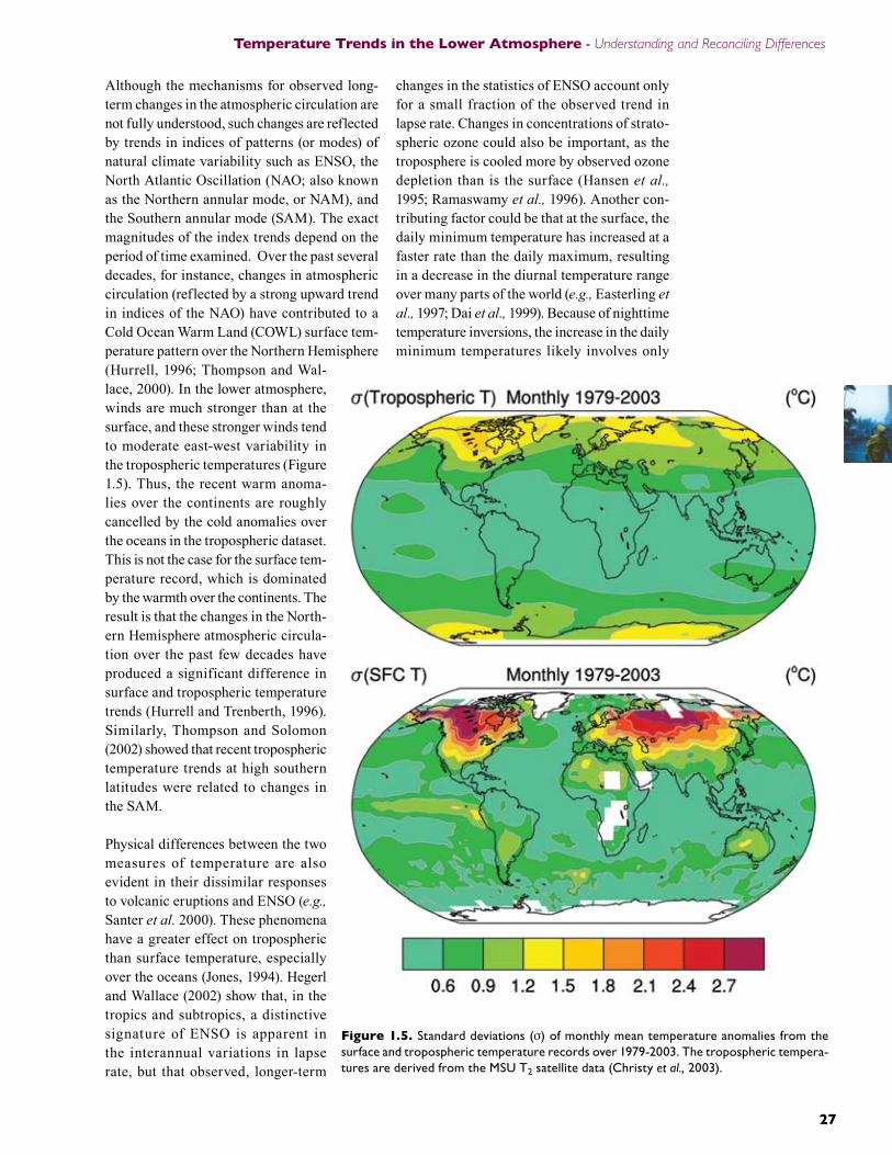
More important than correlations for trends, however, is the variability of the two tem-perature records, assessed by computing the standard deviation of the measurement samples of each record (Figure 1.5). The figure exhibits pronounced regional differences in variability between the surface and tropospheric records. Standard deviations also help in accounting for the differences in correlation coefficients, because they yield information on the size and persistence of the climate signal relative to the noise in the data. For instance, large variations in eastern tropical Pacific sea surface tem-perature associated with ENSO dominate over measurement uncertainties, as do large month-to-month swings in surface temperatures over extratropical continents.

The largest variability in both surface and tropospheric temperature is over the Northern Hemisphere continents. The standard deviation over the oceans in the surface data set is much smaller than over land except where the ENSO

phenomenon is prominent. The standard devia-tions of tropospheric temperature, in contrast, exhibit less zonal variability. Consequently, the standard deviations of the monthly tropospheric temperatures are larger than those of the sur-face data by more than a factor of two over the North Pacific and North Atlantic. Over land, tropospheric temperatures exhibit slightly less variability than surface temperatures. These differences in variability are indicative of dif-ferences in physical processes over the oceans versus the continents. Of particular importance are the roles of the land surface and ocean as the lower boundary for the atmosphere and their very different abilities to store heat, as well as the role of the atmospheric winds that help to reduce regional differences in tropospheric temperature through the movement of heat from one region to another.

Over land, heat penetration into the surface involves only the upper few meters, and the ability of the land to store heat is low. Therefore, land surface temperatures vary considerably from summer to winter and as cold air masses replace warm air masses and vice versa. The result is that differences in magnitude between surface and lower-atmospheric temperature anomalies are relatively small over the conti-

nents: very warm or cold air aloft is usually associated with very warm or cold air at the surface. In contrast, the ability of the ocean to store heat is much greater than that of land, and mixing in the ocean to typical depths of 50 meters or more considerably moderates the sea surface temperature response to cold or warm air. Over the northern oceans, for example, a very cold air mass (reflected by a large negative temperature anomaly in the tropospheric record) will most likely be as-sociated with a relatively small negative temperature anomaly at the sea surface. This is one key to understanding the dif-ferences in trends between the two records.

Figure 1.�. Gridpoint correlation coefficients (r) between monthly surface and tropo-spheric temperature anomalies over 1979-2003. The tropospheric temperatures are derived from the MSU T2 satellite data (Christy et al., 2003).

26 27


26 27

Although the mechanisms for observed long-term changes in the atmospheric circulation are not fully understood, such changes are reflected by trends in indices of patterns (or modes) of natural climate variability such as ENSO, the North Atlantic Oscillation (NAO; also known as the Northern annular mode, or NAM), and the Southern annular mode (SAM). The exact magnitudes of the index trends depend on the period of time examined. Over the past several decades, for instance, changes in atmospheric circulation (reflected by a strong upward trend in indices of the NAO) have contributed to a Cold Ocean Warm Land (COWL) surface tem-perature pattern over the Northern Hemisphere (Hurrell, 1996; Thompson and Wal-lace, 2000). In the lower atmosphere, winds are much stronger than at the surface, and these stronger winds tend to moderate east-west variability in the tropospheric temperatures (Figure 1.5). Thus, the recent warm anoma-lies over the continents are roughly cancelled by the cold anomalies over the oceans in the tropospheric dataset. This is not the case for the surface tem-perature record, which is dominated by the warmth over the continents. The result is that the changes in the North-ern Hemisphere atmospheric circula-tion over the past few decades have produced a significant difference in surface and tropospheric temperature trends (Hurrell and Trenberth, 1996). Similarly, Thompson and Solomon (2002) showed that recent tropospheric temperature trends at high southern latitudes were related to changes in the SAM.

Physical differences between the two measures of temperature are also evident in their dissimilar responses to volcanic eruptions and ENSO (e.g., Santer et al. 2000). These phenomena have a greater effect on tropospheric than surface temperature, especially over the oceans (Jones, 1994). Hegerl and Wallace (2002) show that, in the tropics and subtropics, a distinctive signature of ENSO is apparent in the interannual variations in lapse rate, but that observed, longer-term

Figure 1.5. Standard deviations (σ) of monthly mean temperature anomalies from the surface and tropospheric temperature records over 1979-2003. The tropospheric tempera-tures are derived from the MSU T2 satellite data (Christy et al., 2003).

changes in the statistics of ENSO account only for a small fraction of the observed trend in lapse rate. Changes in concentrations of strato-spheric ozone could also be important, as the troposphere is cooled more by observed ozone depletion than is the surface (Hansen et al., 1995; Ramaswamy et al., 1996). Another con-tributing factor could be that at the surface, the daily minimum temperature has increased at a faster rate than the daily maximum, resulting in a decrease in the diurnal temperature range over many parts of the world (e.g., Easterling et al., 1997; Dai et al., 1999). Because of nighttime temperature inversions, the increase in the daily minimum temperatures likely involves only


28 PB

a shallow layer of the atmosphere that would not be evident in upper-air temperature records. However, during the satellite era, maximum and minimum tempera-tures have been rising at nearly the same rate, so that there has been

almost no change in the diurnal temperature range (Vose et al., 2005).

These physical processes provide indications of why trends in surface temperatures are expected to be different from trends in the troposphere, especially in the presence of strong interannual variability, even if both sets of measurements were perfect. Of course they are not, as de-scribed in more detail in Chapter 2, which deals with the strengths and limitations of current observing systems. An important issue implicit in Figure 1.5 is that of spatial sampling, and the accompanying caveats about interpretation of the truly global coverage provided by satellites versus the incomplete space and time coverage offered by radiosondes. These are discussed in depth in Chapters 2 and 3.

At the surface, the daily minimum temperature increased at a faster rate than the daily maximum since 1958. But since 1979, maximum and minimum temperatures have been rising at nearly the same rate.

temperature trends in the lower atmosphere: steps … · temperature trends in the lower atmosphere...

Documents