Temi di Discussione(Working Papers)

Rethinking the crime reducing effect of education? Mechanisms and evidence from regional divides

by Ylenia Brilli and Marco Tonello

Num

ber 1008A

pri

l 201

5

Temi di discussione(Working papers)

Rethinking the crime reducing effect of education? Mechanisms and evidence from regional divides

by Ylenia Brilli and Marco Tonello

Number 1008 - April 2015

The purpose of the Temi di discussione series is to promote the circulation of working papers prepared within the Bank of Italy or presented in Bank seminars by outside economists with the aim of stimulating comments and suggestions.

The views expressed in the articles are those of the authors and do not involve the responsibility of the Bank.

Editorial Board: Giuseppe Ferrero, Pietro Tommasino, Piergiorgio Alessandri, Margherita Bottero, Lorenzo Burlon, Giuseppe Cappelletti, Stefano Federico, Francesco Manaresi, Elisabetta Olivieri, Roberto Piazza, Martino Tasso.Editorial Assistants: Roberto Marano, Nicoletta Olivanti.

ISSN 1594-7939 (print)ISSN 2281-3950 (online)

Printed by the Printing and Publishing Division of the Bank of Italy

RETHINKING THE CRIME-REDUCING EFFECT OF EDUCATION? MECHANISMS AND EVIDENCE FROM REGIONAL DIVIDES

by Ylenia Brilli* and Marco Tonello**

Abstract

We estimate the contemporaneous effect of education on adolescent crime by exploiting the variation in crime rates between different cohorts and at different ages that followed a reform that raised the school-leaving age in Italy. A 1 percentage-point increase of the enrollment rate reduces adolescent crime by 1.3 per cent in the North of Italy but increases it by 3.9 per cent in the South. The crime-reducing effect depends mainly on incapacitation (i.e. adolescents stay in school instead of on the street); the crime-increasing effect is consistent with a channel of criminal capital accumulation, operating through social interactions and organized-crime networks.

JEL Classification: I20, I28, J13, K42. Keywords: adolescent crime, school enrollment, incapacitation, human capital.

Contents

1. Introduction .......................................................................................................................... 5 2. Institutional background: the 1999 Compulsory Education Reform ................................... 9 3. Identification strategy ......................................................................................................... 11 4. Data and descriptive statistics ............................................................................................ 13 5. Baseline results ................................................................................................................... 18 6. Potential mechanisms ........................................................................................................ 24 7. Conclusions and policy implications ................................................................................. 32 References .............................................................................................................................. 35 Appendix: juvenile delinquency in selected countries ........................................................... 38

______________________________________ * European University Institute. E-mail: ylenia.brilli@eui.eu. ** Bank of Italy, Economics and Statistics Directorate General, Structural Economic Analysis Directorate, Economics and Law Division, and CRELI-Università Cattolica di Milano. E-mail: marco.tonello@bancaditalia.it (corresponding author).

1 Introduction1

In the industrialized countries, increased prosperity and the availability of a growing range of

consumer goods have led to increased opportunities for juvenile crime. With the social changes

that have occurred over the past few decades, the informal traditional control exercised by

adults (including parents, relatives and teachers) over young people has gradually declined, and

adequate substitutes have not been provided (UN, 2003). Juvenile delinquency represents a

sizable share of the overall delinquency rates: in the year 2005 in the US more than 18 percent

of the individuals suspected to have committed a crime were under 18, and this figure was

up to 22 percent in Canada and almost 27 percent in Germany and Sweden.2 Adolescents’

involvement in criminal behaviors is also of a particular policy concern because the victims of

crimes committed by juveniles are mostly other juveniles. Moreover, adolescent crime entails a

high social cost: Cohen and Piquero (2009) estimate that, discounted to present value at birth,

the monetary value of saving a high risk youth ranges between $2.6 and $4.4 millions.

In this paper we consider one characteristic, which has been broadly identified as an im-

portant policy instrument against criminal behavior, i.e. education. Education and school

attendance may affect juvenile crime through several channels (Hjalmarsson and Lochner, 2012,

Jacob and Lefgren, 2003). School may have an incapacitating effect, through which it prevents

adolescents from committing crime, just because criminal opportunities are generally more lim-

ited at schools than on the streets (Anderson et al., 2013). A second mechanism operates through

the improvement of skills, which are remunerated in the labor market and should change the

decisions to engage in criminal activities through a change in the expected probability of finding

a legal job after school completion. This human capital effect may affect youth crime immedi-

ately, but it may also last over time (Lochner and Moretti, 2004, Machin et al., 2011). Finally,

social networks may play a substantive role in shaping adolescent crime, mainly because risky

and criminal behaviors are particularly influenced by peers, especially in the years of adoles-

cence (Bayer et al., 2009, Card and Giuliano, 2013, Patacchini and Zenou, 2009). While the

incapacitation and the human capital channels imply negative effects of education on crime, the

1We are indebted to Giusy Muratore, Pamela Pintus (ISTAT), Angela Iadecola, Gianna Barbieri (Ministryof Education Statistical Office) for making the data available. The paper benefited from comments and sug-gestions of seminar participants at the European University Institute Alumni Conference (Firenze), 26th EALEConference (Ljubljana), Bank of Italy, University of Padova, Catholic University Milan, XXIX AIEL Conferenceof Labour Economics (University of Pisa), X ISLE-SIDE Conference of Law and Economics (University of RomeLa Sapienza). We also thank Andrea Ichino, Claudio Lucifora, Jerome Adda, Francesco Fasani, Mirko Draca,Yarine Fawaz, Paolo Sestito, Effrosyni Adamopoulou, Randi Hjalmarsson, Lucia Rizzica, Silvia Giacomelli, MagdaBianco, Giuliana Palumbo, Monica Andini, Corrado Andini, Pietro Tommasino, Marco Bertoni for useful com-ments. We are grateful to Stefano Marucci and Simone Tonello for research assistance. The views expressed inthis paper are those of the authors and do not necessarily reflect those of the institutions they belong to. YleniaBrilli acknowledges financial support from a Max Weber Fellowship at EUI. The usual disclaimers apply.

2United Nations Survey of Crime Trends and Operations of Criminal Justice Systems, UN-CTS 2005.

5

effects of the social interactions cannot be established a priori as they may either reinforce or

attenuate the individual propensity to engage in risky behaviors.

We examine the empirical relationship between high school attendance and adolescent in-

volvement in criminal activities by exploiting a school leaving age reform, implemented in Italy

in 1999 (hereafter, simply referred to as the Reform), which increased compulsory education by

one year. The Italian context and the 1999 Reform represent an ideal setting for the study of

the effects of education on youth crime and for assessing whether the crime reducing effect of

education, found in several pieces of this literature, might be heterogeneous across the territory

and which underlying channels might help to explain this heterogeneity. In fact, the Reform

was implemented in the same way and with the same rules and timing in the whole country,

which, on the contrary, is characterized by large territorial heterogeneity, both in formal and

informal institutions, tracing back to distant political and historical factors (Barone and Mo-

cetti, 2014, Guiso et al., 2013, Paccagnella and Sestito, 2014). A peculiarity of the Italian case is

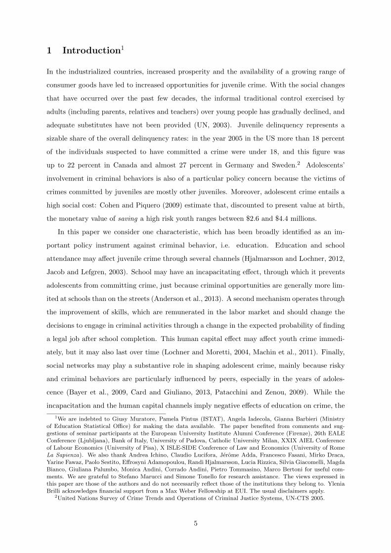
also illustrated in Figure 1, which shows the percentage change in the juvenile rate of suspected

individuals from 1995 to 2003 (i.e. the same time window as the one used in our empirical anal-

ysis, see Section 4). Italy experienced a moderate increasing trend of the juvenile delinquency

rate in the years 1995-2003 (+8.5 percent), while all the other countries (with the exception of

Portugal) recorded low variations (Denmark, Spain, Japan), or even sizable decreases (Sweden,

US, Canada, Germany and Greece).3

Starting from the seminal works of Jacob and Lefgren (2003) and Lochner and Moretti (2004),

several empirical papers have assessed the effects of education on criminal behavior (Lochner,

2011).4 However, only few studies have looked at the contemporaneous effects of educational

policies on adolescent crime and most of them focus on US data (Hjalmarsson and Lochner,

2012).5 Anderson (2013), Bertheleon and Kruger (2011), Luallen (2006) and Jacob and Lefgren

(2003) estimate, in a reduced form setting, the effects of different types of school policies which

induced exogenous variation in the time spent at school by teenagers. Anderson (2013) estimates

that the exposure to a minimum drop-out age of 18 reduces the arrest rate for 16- to 18-year-olds

by 10.27 incidences per 1,000 individuals of the age group population. Bertheleon and Kruger

(2011) find that a school reform that lengthened the time spent at school from half to full-day in

Chilean municipalities significantly decreases youth crime rates and teen pregnancies. Luallen

3This pattern is not observed for adult delinquency, which increases for most of the countries in the sameperiod (with the notable exception of the US, Denmark and Greece).

4Lochner and Moretti (2004) exploit aggregate (state-level) as well as individual-level data and find that schoolattainment significantly reduces the probability of arrest and incarceration of adult males. The work closest toour empirical strategy is that of Machin et al. (2011), which assesses the causal effect of education on adult crimerate exploiting a compulsory leaving age reform implemented during the 70s in the UK. The authors find that a10 percent increase in the average school leaving age lowers crimes of 18 to 40-year-olds by 2.1 percent.

5Only Bertheleon and Kruger (2011) use data from Chile.

6

Figure 1Percentage change in juvenile and adult rates of suspected individuals between 1995 and 2003

NOTES: the graphs shows the percentage change in the rate of suspected individuals (juveniles and adults) between 1995and 2003. Suspected individuals are defined as persons brought into formal contact with the criminal justice system,regardless of the type of crime (where formal contact might include being suspected, arrested, cautioned). Juvenilesare defined as individuals under the age of 18 in all the selected countries except: Sweden (under 21), Portugal (under20), Japan (under 19). Data for the US, Spain, Japan and Greece refer to the year 2005 as the statistics for the years2003 and 2004 are not available. SOURCE: United Nations Survey of Crime Trends and Operations of Criminal JusticeSystems (UN-CTS), United Nations Office for Drugs and Crime (UNODOC) (available at https://www.unodc.org/unodc/en/data-and-analysis/statistics/historic-data.html).

(2006) and Jacob and Lefgren (2003) examine the effects of extra days off from school because

of teachers’ in-service days or teachers’ strikes: Luallen (2006) shows that total juvenile crime

increases by an average of 21.4 percent on days when strikes occur; Jacob and Lefgren (2003)

find that property crimes decrease by 14 percent on days when the school is in session, while

violent crimes increase by 28 percent over the same days. Indeed, the issue of the territorial

heterogeneity of the effects of education on adolescent crime has still found little attention in

the literature. Only Luallen (2006) shows that sizable effects of increasing the number of days

at school on youth crime rates are present in urban and not in rural areas.

This paper contributes to the literature in three significant ways. First, we provide causal

estimates of the contemporaneous effects of high school attendance on adolescent crime. In fact,

we provide both the reduced form effect of the Reform (i.e. the intention-to-treat parameter,

ITT, which is generally found in the existing literature) and the local average treatment effect

(LATE), exploiting the exogenous variation in the enrollment rate induced by the Reform in an

instrumental variable setting. While the ITT may represent the most policy relevant parameter,

only through 2SLS estimation we can provide evidence of the causal link between education

and crime. Second, we show that a crime reducing effect of education is not always present if

the contemporaneous relation between adolescent crime and education is considered (Jacob and

Lefgren, 2003, Luallen, 2006). Third, thanks to the availability of data on school enrollments

and drop-out in the years close to the implementation of the Reform, we also discuss which

7

underlying mechanisms might play a role in explaining our results. Our estimates are based on

newly available administrative records which precisely identify the age of all the offenders and

the province where the offense took place. This means that we can identify not only youths

who have been jailed or arrested, but also all others who have been reported to the judicial

authority and then have benefited from measures alternative to prison, thus reducing the scope

for underestimating the true extent of the phenomenon (Jacob and Lefgren, 2003).

We exploit aggregated administrative records of all 14- and 15-year-olds reported by the

police to the judicial authorities, matched with enrollment rates in the first and second year of

high school to provide causal estimates of the effects of youth enrollment ratio on adolescent

offending rate. We adopt a 2SLS empirical strategy and compare the offending rates of the

cohorts affected by the Reform (our treatment group) with those of the cohorts not affected by

the Reform (our control group). We also exploit this exogenous shift in the enrollment ratio to

retrieve the heterogeneous effects of education on adolescent crime in the different areas of the

country. The empirical evidence we provide is particularly interesting as, differently from other

works establishing causal links between minimum drop-out laws and youth crime, we have the

opportunity to focus on a very recent educational reform.6

While the 1999 Reform increased compulsory education across the whole country by one year,

it determined different effects on adolescent crime in the South than it did in the North. Our

baseline results show that a one percentage point increase in enrollment rate reduces adolescent

offending rate of 14- and 15-year-olds by 1.3 percent in the North, while increasing it by 3.9

percent in the South. The reduced form estimate of the effect of the Reform on the juvenile

offending rate indicates that increasing compulsory education by one year reduces adolescent

crime by 6.9 percent in the North, while increasing it by 13.5 percent in the South. We also

find that the crime reducing effect of education in the North of the country is mainly driven by

the incapacitation effect induced by the Reform. On the contrary, the crime increasing effect

that we find in the South of the country is consistent with a criminal capital accumulation

channel, mainly operating through social interactions and organized-crime networks. Finally, a

human capital accumulation effect of the increase in compulsory education on adolescent crime

is excluded to have played any role in the short run in both areas of the country.

The rest of the paper is organized as follows. Section 2 describes the institutional setting,

Section 3 presents our identification strategy and Section 4 describes the data and provides de-

scriptive statistics. In Section 5 we present the baseline results and we conduct several robustness

and specification checks. Section 6 provides evidence and discusses the potential mechanisms

6For example, Machin et al. (2011) use a school leaving age reform which took place in England and Wales in1972.

8

that could explain our results. Section 7 concludes and derives policy implications.

2 Institutional background: the 1999 Compulsory Education

Reform

The school system in Italy starts with five years of primary school (grades 1 to 5, corresponding

to ISCED level 1) and three years of junior high school (grades 6 to 8, ISCED level 2). These

two compose the first cycle of the school path, which is identical and compulsory for all students.

Secondary education lasts two, three or five years depending on the path chosen (vocational,

technical, academic). Children enroll in the first grade of primary school the year they turn six,

start junior high school when they turn eleven, and enroll in the first grade of high school the

year they turn fourteen. Each student must attend school for at least 8 years and obtain the

junior high school Diploma at the end of the compulsory education path (i.e. at the end of the

first cycle).7

The 1999 Compulsory Education Reform extended compulsory education by one year (from

8 to 9 years). The Reform was aimed at increasing high school attendance and the minimum

drop-out age, which was considered relatively low compared to most European countries (Be-

nadusi and Niceforo, 2010). The direct effect of the Reform was that, starting from the school

year 1998/99, all students enrolled in the 8th grade could not drop-out after the completion of

the junior high school and were obliged to enroll and attend, at least, the first year of high

school. The additional year of education had to be carried out attending lessons in a high school

(academic, technical or vocational), and could not be performed in regional training centers nor

with apprenticeship contracts.

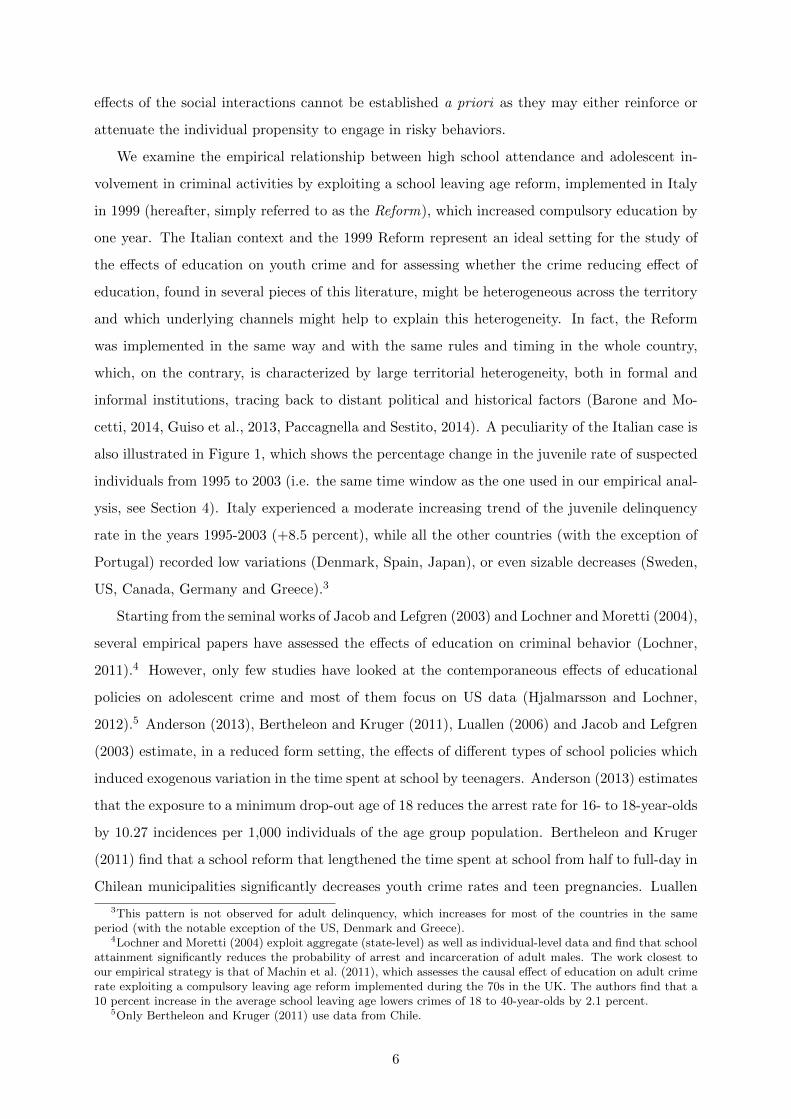
Figure 2 shows the increasing trend of the enrollment ratio for 14- to 18-year-old Italian

adolescents over almost 20 years (from school year 1981/82 to school year 2009/10): a steeper

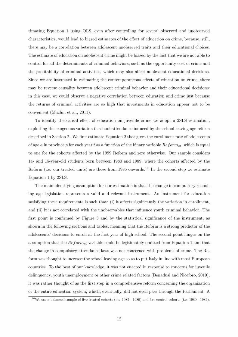
increase can be detected in the years immediately after the introduction of the Reform. Figure 3

shows the increase of the average enrollment ratio of 14- and 15-year-old students (the targeted

group) in the period of implementation of the Reform. The enrollment ratio is obtained as the

share of students enrolled at a certain grade with respect to the corresponding age population.8

The Reform was applied in the same way and with the same timing across the whole country.

This element, together with the richness of the administrative records collected, makes it possible

not only to estimate the empirical relationship between enrollment and crime, but also to study

7This limit was set by the Italian Constitutional Law established in 1948, immediately after World War II.Ordinary laws, as the Reform we are going to illustrate (Law No. 9/1999 and Ministry Decree No. 323/1999),can increase, but not decrease, this minimum drop out age.

8For details, see Section 4.1

9

Figure 2Secondary education enrollment ratio: historical trend

NOTES: the graph shows the historical trend of the enrollment ratio for secondary education (grades 9 to 13). The historicalseries is provided by ISTAT (Italian National Institute of Statistics) and it is calculated as the ratio between the numberof students enrolled in secondary education and the number of resident citizens aged between 14 and 18 (multiplied by100). The circle highlights the school year of the introduction of the 1999 Reform, the vertical lines delimit the period ofobservation used in the empirical analysis. SOURCE: ISTAT, Historical Series.

Figure 3Trends in the enrollment ratio of 14- and 15-year-olds

NOTES: the graph shows the average enrollment ratio of 14- and 15-year-old students (grades 9 and 10) by cohort. Thevertical line denotes the first cohort affected by the 1999 Reform. SOURCE: own elaborations from ISTAT and MIUR.

10

how the same policy prescription could have had differential effects on adolescent crime across

the territory and which underlying channels might help to explain such differences.

3 Identification strategy

Our aim is to estimate the causal effect of education on adolescent crime. The identification

strategy considers the following equations:

Crimeapt = θ0 + θ1Eduapt + θ2Xapt + θ3Wpt + (1 + ηj)φt + ωp + ωa + ta + νapt (1)

Eduapt = δ0 + δ1Reformat + δ2Xapt + δ3Wpt + (1 + ηj)φt + ωp + ωa + ta + εapt (2)

where Crimeapt represents a measure of the criminal activity of the teenagers of age a living

in province p in year t, and Eduapt represents an educational measure of the teenagers of age a

living in province p in year t; in the baseline estimation we consider adolescents aged 14 and 15.9

The vector Xapt includes control variables at province level varying over time and age group,

while the vector Wpt includes socio-economic indicators referred to each province p in each

year t. More precisely, we control for several socio-economic characteristics, which have been

considered potential determinants of juvenile crime by the existing literature (Anderson, 2013,

Machin et al., 2011): the vector Xapt includes demographic variables (i.e. the share of youth

living in an urban area), while the vector Wpt includes the average labor force participation rate

for 15- to 24-year-olds, which is intended to proxy for the (legal) labor market opportunities, the

(natural logarithm of) provincial per capita value added as a proxy for the general level of wealth

in each province, and the (natural logarithm of) provincial population, which, in combination

with province fixed effects, implicitly controls for population density.

In order to control for time invariant unobserved heterogeneity in provincial characteristics

and for annual trends in adolescent crimes, we use year (φt) and province (ωp) fixed effects.

We also include age fixed effects (ωa) and age-specific linear time trends (ta), to control for the

different propensity to commit crime across ages (Nagin and Land, 1993), and to account for

time series variation particular to each age. Finally, we add the interaction between year fixed

effects and regional fixed effects (ηj), to capture relevant territorial dynamics which cannot be

included in the vector of control variables, such as macro shocks to the economy which may have

different impacts in the areas of the country or population dynamics.

Equation 1 describes the contemporaneous relationship between education and crime. Es-

9That is: a ∈ [14; 15]; Italian regions correspond to NUTS 2 level (j = 1 . . . 19), each region includes a variablenumber of provinces (NUTS 3 level, p = 1 . . . 91). See Section 4.1 for the detailed description of the educationand crime measures used.

11

timating Equation 1 using OLS, even after controlling for several observed and unobserved

characteristics, would lead to biased estimates of the effect of education on crime, because, still,

there may be a correlation between adolescent unobserved traits and their educational choices.

The estimate of education on adolescent crime might be biased by the fact that we are not able to

control for all the determinants of criminal behaviors, such as the opportunity cost of crime and

the profitability of criminal activities, which may also affect adolescent educational decisions.

Since we are interested in estimating the contemporaneous effects of education on crime, there

may be reverse causality between adolescent criminal behavior and their educational decisions:

in this case, we could observe a negative correlation between education and crime just because

the returns of criminal activities are so high that investments in education appear not to be

convenient (Machin et al., 2011).

To identify the causal effect of education on juvenile crime we adopt a 2SLS estimation,

exploiting the exogenous variation in school attendance induced by the school leaving age reform

described in Section 2. We first estimate Equation 2 that gives the enrollment rate of adolescents

of age a in province p for each year t as a function of the binary variable Reformat, which is equal

to one for the cohorts affected by the 1999 Reform and zero otherwise. Our sample considers

14- and 15-year-old students born between 1980 and 1989, where the cohorts affected by the

Reform (i.e. our treated units) are those from 1985 onwards.10 In the second step we estimate

Equation 1 by 2SLS.

The main identifying assumption for our estimation is that the change in compulsory school-

ing age legislation represents a valid and relevant instrument. An instrument for education

satisfying these requirements is such that: (i) it affects significantly the variation in enrollment,

and (ii) it is not correlated with the unobservables that influence youth criminal behavior. The

first point is confirmed by Figure 3 and by the statistical significance of the instrument, as

shown in the following sections and tables, meaning that the Reform is a strong predictor of the

adolescents’ decisions to enroll at the first year of high school. The second point hinges on the

assumption that the Reformat variable could be legitimately omitted from Equation 1 and that

the change in compulsory attendance laws was not concerned with problems of crime. The Re-

form was thought to increase the school leaving age so as to put Italy in line with most European

countries. To the best of our knowledge, it was not enacted in response to concerns for juvenile

delinquency, youth unemployment or other crime related factors (Benadusi and Niceforo, 2010);

it was rather thought of as the first step in a comprehensive reform concerning the organization

of the entire education system, which, eventually, did not even pass through the Parliament. A

10We use a balanced sample of five treated cohorts (i.e. 1985 - 1989) and five control cohorts (i.e. 1980 - 1984).

12

validity threat for our identification strategy also relates to the potential correlation between

unobserved crime determinants and time-varying area-specific unobserved characteristics also

influencing enrollment decisions, if these are contemporaneous to the implementation of the Re-

form. For this reason, in all the specifications we control for region by year fixed effects, which

allow to get rid of time-varying and area-specific phenomena. Finally, it should be acknowledged

that the variation induced by the instrument is very likely to be local, since it has an impact

only on the bottom of the education measure distribution and not at the top. When we estimate

the parameter θ1 using 2SLS, we are identifying a local average treatment effect (LATE), since

only adolescents at the margin between dropping out and continuing education are affected by

the policy in their educational decisions.

In the empirical analysis, we also estimate a reduced form model of the effects of the 1999

Reform on crime, which takes the following specification:

Crimeapt = β0 + β1Reformat + β2Xapt + β3Wpt + (1 + ηj)φt + ωp + ωa + ta + ςapt (3)

The estimate from the crime reduced form (RF) (i.e. β1 in Equation 3) can be interpreted as

an intention-to-treat (ITT) effect providing an overall estimate of the consequences on adoles-

cent crime of raising compulsory education by one year, and representing the relevant policy

parameter. Moreover, lacking specific or aggregated measures of school enrollment, this is the

parameter usually estimated in the existing literature on the contemporaneous effects of school

attendance on juvenile delinquency.

4 Data and descriptive statistics

4.1 Data and variables construction

We collect data on the number of offenders reported to the judicial authority and high school

enrollments, for 14- and 15-year-old adolescents in the years before and after the implementation

of the Reform. Our dataset is thus composed by cells defined by the year (from 1995 to 2003),

the age, and the province.11 In the baseline empirical analysis we consider a time span covering

nine school years, while in a later section we also check the robustness of our results using a

11Since the number of provinces in Italy increased dramatically during the 90s, to maintain consistency of thedata across years, we use the ISTAT definition of 95 provinces. Four provinces are dropped from the analysis:three of them because part of Autonomous Regions (i.e. Val d’Aosta, Trentino and Alto Adige) which followed adifferent implementation of the Reform, one (Oristano) because of missing data.

13

smaller time window.12

For each cell, we construct a measure of the involvement in criminal activity based on the

Italian National Institute of Statistics (ISTAT) official data on adolescent offenders. The ISTAT

data on adolescent offenders have the unique characteristic of offering aggregate measures of the

number of teenagers reported to the judicial authority for whom we know the exact age.13 Our

measure of criminal activity (i.e. the Offending Rate, OR) is then the number of adolescents

reported by the police to the judicial authority (offendersapt) over the corresponding age-year-

province population (Popapt):

ORapt =offendersaptPopapt

× 1, 000 (4)

where p indexes the province, a the age, and t the year. Notice that the use of the number

of adolescents reported by the police to the judicial authority is likely to be a more accurate

measure of the involvement of teenagers in criminal activities. As outlined by Jacob and Lefgren

(2003) and Machin et al. (2011), alternative measures, such as crime rates based on the number of

crimes committed, would not be as accurate in the definition of the exact age of the offender. On

the other hand, arrest rates obtained from the number of teenagers arrested could significantly

underestimate the true magnitude of the phenomenon, as we also documented in the Appendix

Table A.1. Finally, the use of provincial and year fixed effects in all the empirical specifications

limit any systematic measurement error due to underreporting constant within geographical

areas (over time) or within periods (across areas) (Bianchi et al., 2012).

In order to measure the enrollment ratio of the cohorts relevant for our analysis, we collect

data on the number of students enrolled in high schools in each province for the school years

1995/96 to 2003/04, from the Statistical Office of the Italian Ministry of Education (MIUR). We

focus on 14- and 15-year-old students as they represent the age group targeted by the Reform.

We define the Enrollment Ratio (ER) as the number of adolescents who are enrolled in secondary

education (enrollmentsapt) over the corresponding age-year-province population (Popapt):

ERapt =enrollmentsapt

Popapt(5)

We then merge the two datasets by year, age and province cells and link socio-economic informa-

12Starting from 2004 a new comprehensive educational reform was introduced and, among other things, theminimum drop-out age was reduced to the Constitutional limit in force before the 1999 Reform. For this reason,we focus our empirical analysis on a balanced time window (before and after the introduction of the Reform) inthe years before 2004.

13ISTAT data on juvenile offenders are also available for 16- and 17-year-olds, while not for children aged 13 andbelow, because they cannot be formally sent to jail (Dipartimento di Giustizia Minorile, 2007). We will exploitthis data in a later section.

14

tion at the province level from different data sources, such as the Labor Force Survey (ISTAT),

the Public Finance Database (Italian Ministry of Interior), the Italian Demographic Database

(ISTAT).14

4.2 Descriptive statistics

In Section 2 we describe the introduction of the Reform, and illustrate the effects it determined

in the historical trend of the enrollment ratio. In this section we go deeper into the descriptive

analysis of the effects of the Reform both on the side of the educational outcomes (i.e. the

enrollment ratio of 14- and 15-year-olds) and on the side of the dependent variable (i.e. the

offending rate of 14- and 15-year-olds).

Table 1Descriptive statistics

mean sd max min N

Offending rate (OR) (overall) 10.41 6.06 56.50 0.00 1638Offending rate: North 11.30 6.87 56.50 0.00 1044Offending rate: South 8.86 3.82 24.31 0.00 594Enrollment ratio (ER) (overall) 0.95 0.08 1.00 0.43 1638Enrollment rate: North 0.96 0.07 1.00 0.43 1044Enrollment rate: South 0.94 0.08 1.00 0.70 594Urban share 0.13 0.19 0.87 0.00 1638Occupation rate (15-24) 31.10 10.44 49.60 12.07 1638Provincial per capita VA 14481.54 6487.91 45165.42 5148.52 1638Provincial population 613731.79 643997.04 3980000 89775 1638

NOTES: offending rates are calculated per 1,000 of the corresponding province-age population. Urban share refers to theshare of youth living in an urban area, Occupation rate (15-24) is the the average occupation rate for 15- to 24-year-olds,provincial per capita VA refers to the provincial per capita value added (in 2012 Euros), provincial population refers to thetotal provincial population. SOURCE: ISTAT and ISTAT-Demos.

Table 1 contains general descriptive statistics on the dependent and control variables included

in the empirical specifications. The average enrollment ratio is equal to 0.95, while the average

offending rate is of 10.41 adolescents reported to the judicial authority per 1,000 individuals

of the corresponding age group population. The Reform increased by 6.3 percent the overall

enrollment ratio: the raw increase in the enrollment ratio is slightly higher in the South (+8.2

percent) than in the North (+5.4 percent) of the country. This is probably due to the fact that

the two areas started from different initial levels of adolescent enrollment in high schools (lower

in the South than in the North) and rapidly converge after the implementation of the Reform.

Figure 4 shows the geographical distribution across Italian provinces of the average offending

rate in the years used in the empirical analysis. Higher levels are recorded in the Northern

provinces and in the provinces with the main urban areas (e.g. Milan, Rome, Turin, Naples,

Palermo). In Figure 5, we show the average residuals from OLS regressions where the dependent

14The match between the two measures is such that, for example, the enrollment ratio for the school year1995/96 is linked to the offending rates of the year 1995.

15

Figure 4Geographical distribution of the offending rate of 14- and 15-year-olds

NOTES: the map shows the average offending rate of 14- and 15-year-olds over the period 1995-2003 (rates expressed per1,000 of the corresponding age group population). SOURCE: own elaborations from ISTAT.

variable is the offending rate and we include as regressors province and year fixed effects; the

vertical lines denote the implementation of the Reform. Apparently, the introduction of the

Reform does not determine a dramatic change in the pattern of the residuals (Figure 5.A).

However, plotting the residuals distinguishing between the North and the South of the country

makes it possible to uncover an interesting pattern (Figure 5.B): at the time of implementation

of the Reform, the offending rate experiences a remarkable decrease in the North of the country,

both for 14- and 15-year-olds, while the opposite occurs in the South, where a sharp increase

can be detected. This descriptive evidence highlights crucial differences in the way in which

juvenile delinquency reacted to the increase of the school leaving age between the two areas of

the country that we aim to analyze in depth in the next section.

16

Figure 5Regional divides in the trends of the offending rates (residuals) by age

NOTES: the graphs show the average residuals from OLS regressions of the offending rates (indicated as OR (residuals) onthe vertical axes) on year and province fixed effects. Panel (A) shows the overall trend for 14- and 15-year-olds; Panel (B)shows the trends for 14- and 15-year-olds, separately for the North and the South of the country. The vertical line denotesthe first cohort affected by the 1999 Reform. SOURCE: own elaborations from ISTAT.

17

5 Baseline results

5.1 The contemporaneous effect of education on adolescent crime

We estimate Equation 1 using a 2SLS regression, with robust standard errors clustered at the

province level and weights equal to the corresponding age-year-province population.15

Table 2Contemporaneous effects of education on adolescent crime: baseline results

(1) (2) (3) (4) (5) (6) (7) (8) (9) (10)

OLS First stage 2SLS Reduced Form

ER -1.59 -1.35 -0.82 4.66 2.65 2.79(2.56) (1.72) (1.78) (5.27) (7.40) (7.51)

Reform 0.04*** 0.31 0.12 0.12(0.01) (0.35) (0.34) (0.35)

First stage F-stat. 192.90 34.53 33.50N.Clusters 91 91 91 91 91 91 91 91 91 91N.Observations 1638 1638 1638 1638 1638 1638 1638 1638 1638 1638

Province, year, age FE, age trend yes yes yes yes yes yes yesRegion by year FE yes yes yes yes yes yes yesControl variables yes yes yes yes

NOTES: population weighted models estimated on age-year-province cells. The dependent variable of the 2SLS and reducedform models is the offending rate of 14- and 15-year-olds (OR); the dependent variable of the first stage regression is theenrollment ratio (ER) of 14- and 15-year-olds. Control variables include the share of youth living in an urban area (Urbanshare), the average occupation rate for 15-24 year-olds (Occupation rate (15-24)), the logarithm of the provincial per capitavalue added (2012 Euros) (ln(provincial per capita VA)), the logarithm of provincial population (ln(provincial population)).The First stage F-stat. refers to the Kleibergen-Paap rk Wald F-statistics. Robust standard errors in parenthesis, clusteredat the province level. Asterisks denote statistical significance at the * p < 0.1, ** p < 0.05, *** p < 0.01 levels.

Table 2 shows our baseline results. Columns (1), (2) and (3) contain the estimates of the

parameter θ1 from Equation 1 using OLS regressions, where we progressively add the fixed

effects (column 2) and the control variables (Xapt and Wpt, column 3). Results show a negative,

but not statistically significant correlation, between the ER and the adolescent offending rate.

Column (4) presents the results from the first stage regression where we test the relevance of

our instrumental variable (Reformat in Equation 2). The coefficient is positive and statistically

significant, meaning that the 1999 Reform induced a significant increase in the enrollment ratio of

14- and 15-year-olds, while the first stage F-statistics lies above the thresholds specified by Stock

and Yogo (2005), ensuring that estimates from the 2SLS regressions are not poorly identified.

Columns (5), (6) and (7) contain the results from the 2SLS estimates: even if the model is well

identified, we do not detect statistically significant effects. Similar results hold for the reduced

form estimates (Equation 3) contained in columns (8), (9) and (10). Thus, considering the

whole country, we find that the Reform had a positive effect on the enrollment ratio but we

do not uncover any effects on the adolescents’ offending rate, neither in the 2SLS, nor in the

reduced form framework. However, the descriptive patterns illustrated in Figure 5 guide us to

a deeper analysis considering separately the subsamples of provinces located in the North and

15The use of population weighted models increase the statistical precision of the estimates. The results arerobust to the use of alternative weights and to the exclusion of weights (see Section 5.2).

18

in the South of the country.

Table 3Contemporaneous effects of education on adolescent crime: territorial divide

(1) (2) (3) (4) (5) (6) (7) (8) (9)

First stage 2SLS Reduced FormOverall North South Overall North South Overall North South

ER 2.79 -15.12** 34.98***(7.51) (6.82) (12.13)

Reform 0.04*** 0.05*** 0.03*** 0.12 -0.78* 1.20***(0.01) (0.01) (0.01) (0.35) (0.45) (0.40)

First stage F-stat. 33.50 17.17 29.75N.Clusters 91 58 33 91 58 33 91 58 33N.Observations 1638 1044 594 1638 1044 594 1638 1044 594Control variables and FE yes yes yes yes yes yes yes yes yes

NOTES: population weighted models estimated on age-year-province cells. The dependent variable of the 2SLS and reducedform models is the offending rate of 14- and 15-year-olds (OR); the dependent variable of the first stage regressions is theenrollment ratio (ER) of 14- and 15-year-olds. Control variables include the share of youth living in an urban area (Urbanshare), the average occupation rate for 15-24 year-olds (Occupation rate (15-24)), the logarithm of the provincial percapita value added (2012 Euros) (ln(provincial pc VA)), the logarithm of provincial population (ln(provincial population));the fixed effects (FE) are the ones indicated in Table 2 The First stage F-stat. refers to the Kleibergen-Paap rk WaldF-statistics. Robust standard errors in parenthesis, clustered at the province level. Asterisks denote statistical significanceat the * p < 0.1, ** p < 0.05, *** p < 0.01 levels.

The 2SLS (columns 4-6) and the crime reduced form estimates (columns 7-9) in Table 3

show opposite results, revealing that there exists a crime reducing effect of education only

in the Northern provinces, and that the Reform increased adolescent crime in the Southern

ones. Specifically, an increase in the enrollment ratio (ER) by one percentage point determines

a decrease in the offending rate of 15 incidences per 1,000 of the corresponding age group

population in the North, while it determines an increase of 35 incidences in the South. In absolute

terms, an increase by one percentage point of the enrollment ratio reduces the offending rate by

almost 1.3 percent in the North, while increasing it by 3.9 percent in the South. Similar results

hold for the reduced form equation: one additional year of compulsory education reduces the

offending rate of 14- and 15-year-olds by 0.78 incidences per 1,000 of the corresponding age group

population in the North, while increasing it by 1.2 incidences in the South. In relative terms,

they represent, respectively, a 6.9 percent decrease and a 13.5 percent increase of the offending

rate. Notice also that the reduced form coefficients are slightly larger (in absolute value) than

the corresponding 2SLS estimates, since they may incorporate any indirect or spillover effect of

the Reform.

The crime reducing effect we find in the North of the country is in line with Anderson (2013),

who finds that the exposure to a minimum drop-out age of 18 reduces the arrest rate for 16- to

18-year-olds by 17.2 percent. Also the crime increasing effect is not new in the literature on the

contemporaneous effects of school attendance on crime: Jacob and Lefgren (2003) and Luallen

(2006) find that the level of property crime committed by juveniles decreases when school is in

session, while the level of violent crime increases in the same days.

19

In order to understand these results, one should also bear in mind that incapacitation (i.e.

the additional time to be spent at school) is not the only mechanism with which enrollment might

affect crime. Another mechanism that applies to this framework is the human capital effect,

according to which the time spent at school contributes to increase the opportunity cost of

committing a crime and enlarges the set of labor market opportunities that adolescents can find

in the legal labor market. Finally, there might be an important role played by social interactions,

even if it is not clear in which direction they could affect crime. For instance, staying at school an

additional year may force adolescents with more propensity to commit crime to face their peers

with lower criminal propensity and this may negatively affect their criminal behavior, either

contemporaneously or over time. However, if adolescents at school only interact with bad peers

engaged in criminal activities, this could reinforce, instead of decrease, the youth crime rate.

In Section 6, we will explore these potential mechanisms to explain whether they could have

determined the different effects we observed across the Italian territory. Before doing this, in

the following section we perform several robustness and sensitivity analysis to test the reliability

of our baseline results.

5.2 Robustness and specification tests

As a first test of the robustness of our results, we take advantage of additional data that we

collected for the crime and education measures in the years before the implementation of the

Reform to perform a placebo exercise. In detail, we rerun our baseline regressions as if the

Reform were implemented in the school year 1995/96 (instead of 1999/00), and thus contrasting

the behaviors of adolescents born between 1981 and 1984 (our placebo treated group) with those

born between 1977 and 1980 (our placebo control group).16

In Table 4 Panel A we present the results of a specification including the full set of fixed

effects: the placebo reform does not have any statistically significant effect on the adolescent

offending rate, neither overall nor in the two areas of the country, thus confirming the goodness of

the identification strategy. In Table 4 Panel B we also include the time-varying control variables

(Xapt and Wpt). The inclusion of the control variables shrinks the number of observations: this

is because some variables (i.e. the value added and the occupation rate) are not available for

years before 1995 at the province level. The estimates are still not statistically different from

zero.

Then, we test the robustness of our estimates over several dimensions and report the results

16In this way, we exclude from the placebo exercise adolescents who were really affected by the Reform (i.e.those born in 1985 and afterwords). Since crime measures for older cohorts are not available, we use eight cohortsin the placebo instead of the ten cohorts used in the main analysis (i.e. N = 1, 365).

20

Table 4Placebo exercise

(1) (2) (3) (4) (5) (6) (7) (8) (9)

First stage 2SLS Reduced Form

Panel A Overall North South Overall North South Overall North South

ER 27.77 11.63 -43.93 0.29 0.28 0.30(58.74) (23.29) (50.61) (0.29) (0.43) (0.41)

Reform 0.01 0.02 -0.01(0.02) (0.04) (0.00)

First stage F-stat. 0.23 0.40 2.38N.Clusters 91 58 33 91 58 33 91 58 33N.Observations 1365 870 495 819 522 297 819 522 297Fixed Effects yes yes yes yes yes yes yes yes yes

Panel B Overall North South Overall North South Overall North South

ER 20.34 9.19 -275.96(25.93) (13.99) (757.26)

Reform 0.02 0.04 -0.00 0.37 0.33 0.49(0.02) (0.04) (0.01) (0.32) (0.49) (0.41)

First stage F-stat. 0.63 0.79 0.09N.Clusters 91 58 33 91 58 33 91 58 33N.Observations 819 522 297 819 522 297 819 522 297Fixed Effects yes yes yes yes yes yes yes yes yesControl variables yes yes yes yes yes yes yes yes yes

NOTES: population weighted models estimated on age-year-province cells. The dependent variable of the 2SLS and reducedform models is the offending rate of 14- and 15-year-olds (OR). For the control variables and the fixed effects (FE) includedin the specification see Table 2. The First stage F-stat. refers to the Kleibergen-Paap rk Wald F-statistics. Robust standarderrors in parenthesis, clustered at the province level. Asterisks denote statistical significance at the * p < 0.1, ** p < 0.05,*** p < 0.01 levels.

in Table 5. The main analysis is performed considering a period of time ranging between the

school years 1995/96 and 2003/04, with five cohorts affected by the Reform and five cohorts

unaffected. However, it could be that the longer the period of time used in the empirical

specification, the more difficult it is to satisfy the main assumptions used for identification,

namely the comparability between cohorts. To test for this, we repeat the estimation keeping

only seven school years, from 1996/97 to 2002/03. The results presented in Table 5, specification

1, are close to our baseline (Table 3): 2SLS coefficients are marginally larger, confirming that

identification comes prevailingly from variation close to the discontinuity induced by the Reform.

Specifications 2, 3 and 4 of Table 5 implement different weighting schemes. Specification 2

shows the baseline estimates without weights: as expected, results deliver point estimates similar

to the baseline, albeit less precisely estimated. Specification 3 implements a scheme in which

more weight is given to the cohorts closer to the year of implementation of the Reform and to

14-year-old students, i.e. those directly affected (Inverse Distance Weighting, IDW, see Machin

et al. (2011)).17 As for specification 1, the coefficients are marginally larger, in absolute terms,

with respect to the baseline. Specification 4 includes IDW interacted with population weights:

17IDW are constructed as follows: IDW = (1/d)×W , where d is the distance in birth years from the discon-tinuity, and W is equal to 2 for 14-year-olds, and 1 for 15-year-olds.

21

Table 5Robustness checks

(1) (2) (3) (4) (5) (6)

2SLS Reduced Form

Specification 1 Overall North South Overall North South

ER 1.17 -19.17*** 39.17***(8.22) (7.09) (14.68)

Reform 0.05 -0.90** 1.20***(0.35) (0.44) (0.42)

First stage F-stat. 25.97 13.27 23.15N.Clusters 91 58 33 91 58 33N.Observations 1274 812 462 1274 812 462

Specification 2 Overall North South Overall North South

ER 0.65 -12.69 30.74*(9.72) (12.04) (16.66)

Reform 0.02 -0.52 0.99*(0.40) (0.53) (0.55)

First stage F-stat. 54.79 34.57 20.42N.Clusters 91 58 33 91 58 33N.Observations 1638 1044 594 1638 1044 594

Specification 3 Overall North South Overall North South

ER 0.30 -16.60** 35.90***(7.46) (7.07) (13.41)

Reform 0.01 -0.87* 1.07***(0.34) (0.46) (0.38)

First stage F-stat. 37.45 22.48 22.88N.Clusters 91 58 33 91 58 33N.Observations 1638 1044 594 1638 1044 594

Specification 4 Overall North South Overall North South

ER 0.43 -16.70** 35.21***(7.36) (6.97) (12.99)

Reform 0.02 -0.88* 1.08***(0.34) (0.46) (0.38)

First stage F-stat. 38.36 22.42 24.64N.Clusters 91 58 33 91 58 33N.Observations 1638 1044 594 1638 1044 594Control variables and FE yes yes yes yes yes yes

NOTES: population weighted models estimated on age-year-province cells. The dependent variable of the 2SLS and reducedform models is the offending rate of 14- and 15-year-olds (OR). For the control variables and the fixed effects (FE) includedin the specification see Table 2. Specification 1 conducts the analysis on a time window of 7 years; Specification 2 showsthe baseline specification without weights; Specification 3 implements inverse distance weights (IDW); Specification 4implements inverse distance weights interacted with population weights. The First stage F-stat. refers to the Kleibergen-Paap rk Wald F-statistics. Robust standard errors in parenthesis, clustered at the province level. Asterisks denote statisticalsignificance at the * p < 0.1, ** p < 0.05, *** p < 0.01 levels.

22

the results do not substantially differ from specification 3.

Table 6Sensitivity tests

(1) (2) (3) (4) (5) (6)

2SLS Reduced Form

Specification 1 Overall North South Overall North South

ER 2.74 -15.35** 35.28***(7.59) (6.91) (12.30)

Reform 0.12 -0.78* 1.20***(0.35) (0.45) (0.40)

First stage F-stat. 33.30 17.13 28.39N.Clusters 91 58 33 91 58 33N.Observations 1638 1044 594 1638 1044 594

Specification 2 Overall North South Overall North South

ER 1.90 -14.58** 32.36***(7.25) (6.95) (11.68)

Reform 0.08 -0.76* 1.09***(0.32) (0.44) (0.38)

First stage F-stat. 40.26 20.83 31.04N.Clusters 91 58 33 91 58 33N.Observations 1638 1044 594 1638 1044 594

Specification 3 Overall North South Overall North South

ER 2.84 -14.91** 34.07***(7.41) (6.76) (11.56)

Reform 0.13 -0.78* 1.21***(0.35) (0.45) (0.40)

First stage F-stat. 34.86 17.40 32.52N.Clusters 91 58 33 91 58 33N.Observations 1638 1044 594 1638 1044 594

Control variables and FE yes yes yes yes yes yes

NOTES: population weighted models estimated on age-year-province cells. The dependent variable of the 2SLS and reducedform models is the offending rate of 14- and 15-year-olds (OR). For the control variables and the fixed effects included inthe baseline specification see Table 2. Specification 1 excludes from the baseline specification the age trends; Specification2 adds to the baseline specification regional linear time trends; Specification 3 adds to the baseline specification regionby age fixed effects. The First stage F-stat. refers to the Kleibergen-Paap rk Wald F-statistics. Robust standard errorsin parenthesis, clustered at the province level. Asterisks denote statistical significance at the * p < 0.1, ** p < 0.05, ***p < 0.01 levels.

Finally, we perform a set of sensitivity checks for the specification used in the baseline

analysis, reporting the results in Table 6. Age-specific time trends are added in the baseline

specification to account for time series variation particular to each age; specification 1 of Table

6 relaxes this assumption and shows the estimates of the baseline model excluding them. In the

baseline analysis, the region by year fixed effects account for time-variant unobserved factors.

However, each region can be characterized by its own time trend for adolescent offending rates,

and specification 2 controls for region-specific time trends. Specification 3 adds age-by-region

fixed effects that can be included in the model to allow for separate shifts in the offending

rates of 14- and 15-year-olds in different regions. The results for the three specifications do not

23

significantly differ from the estimates of the baseline model.18

We perform additional specification tests concerning the functional form chosen for the re-

gression model (results available upon request). As in most of the existing literature, we exploit

OLS regressions which allow to estimate in a flexible and robust way instrumental variable mod-

els. However, our results do not change defining the dependent variable as the natural logarithm

of the offending rate and replacing a zero when the logarithm is not defined (Bianchi et al., 2012,

Fougere et al., 2009, Oster and Agell, 2007). It is also widely recognized that crime measures

have a count-data nature and might be appropriately estimated with count-data models (Jacob

and Lefgren, 2003, Luallen, 2006, Osgood, 2000): our reduced form results are also robust to

the use of negative binomial and Poisson regressions.

6 Potential mechanisms

As a matter of fact, the same treatment induced by the Reform had differential effects across

the territory and this could be plausibly due to the relative role that the channels highlighted

above might play in the different areas of the country. In what follows, we provide evidence on

the underlying mechanisms that are likely to explain our results.

6.1 The human capital channel

Additional years of compulsory education might affect youth criminal behavior through a human

capital accumulation effect, that is, staying longer at school should increase the expected value

of a future wage, as well as skill acquisition and the subsequent expectation of finding a job.

Moreover, additional school time could also convey social values and, in general, modify the

individuals’ time preferences and expectations (Lochner, 2011). All these elements are likely to

reduce juvenile delinquency, through an increase in the expected cost of committing a crime.

If a human capital effect is at work we should expect the crime reducing effect of education

to propagate in the years immediately after the school leaving age.19 The relevance of this

channel in our context can be assessed extending our empirical analysis exploiting the crime and

education measures collected for 16- and 17-year-olds. In this case, we compare the same group

of cohorts as the ones used in the main specification, but focusing on the offending rates when

they are one or two years older. The results are presented in Panel A of Table 7. Overall, we

18The results are also robust to alternative clustering (i.e. at the cohort and at the cohort by province level).Estimates are available upon request from the authors.

19Notice that seminal works on the crime reducing effect of education focus on the human capital channel atlater ages (e.g. 18- to 40-year-olds for Machin et al. (2011); 20- to 60-year-olds for Lochner and Moretti (2004)).Thus, our exercise does not discard a human capital effect later in life, rather it focuses on the years immediatelyafter compulsory education.

24

Table 7Potential mechanisms: human capital accumulation and incapacitation

(1) (2) (3) (4) (5) (6) (7) (8) (9)

First stage 2SLS Reduced Form

Panel A Overall North South Overall North South Overall North South

ER 42.41 -1.72 –(34.59) (24.94) –

Reform 0.01*** 0.03*** -0.00 0.53 -0.04 1.19**(0.00) (0.01) (0.01) (0.41) (0.61) (0.55)

First stage F-stat. 10.60 19.10 –N.Clusters 91 58 33 91 58 – 91 58 33N.Observations 1638 1044 594 1638 1044 – 1638 1044 594

OLS First stage 2SLS

Panel B Overall North South Overall North South Overall North South

ER (Net) -2.60 -4.65** -0.27 2.36 -11.56** 49.47**(1.78) (2.11) (2.25) (6.90) (5.78) (23.15)

Reform 0.05*** 0.06*** 0.03***(0.01) (0.01) (0.01)

First stage F-stat. 46.88 73.47 10.66N.Clusters 91 58 33 91 58 33 91 58 33N.Observations 1638 1044 594 1638 1044 594 1638 1044 594

Control variables and FE yes yes yes yes yes yes yes yes yes

NOTES: population weighted models estimated on age-year-province cells. The dependent variable of the 2SLS and reducedform models is the offending rate (OR); the dependent variable of the first stage regressions is the enrollment ratio (ER).Panel A shows the estimates on 16- and 17-year-olds; Panel B shows the estimates using the enrollment ratio net of studentsdropped-out. This is obtained excluding from the number of students enrolled in each grade the fraction of students dropped-out during the school year. For the control variables and the fixed effects included see Table 2. The First stage F-stat.refers to the Kleibergen-Paap rk Wald F-statistics. Robust standard errors in parenthesis, clustered at the province level.Asterisks denote statistical significance at the * p < 0.1, ** p < 0.05, *** p < 0.01 levels.

do not find effects on 16- and 17-year-olds offending rates, both in the 2SLS and reduced form

estimates (columns 4 and 7), although the estimates of the first stage regressions (columns 1,

2 and 3) indicate that the the Reform continued to have some minor effects in increasing the

enrollment ratio, but in Northern regions only.

Concerning the subsamples corresponding to the two areas of the country, the 2SLS estimates

are identified for the Northern subsample only (column 5), which, however, does not show any

statistical significant effect, also in the reduced form estimates (column 8). In the Southern

provinces, the cohorts treated by the Reform do not increase their enrollment in the years

after the compulsory path ends, so that the 2SLS estimation is not even identified (column 6).

Estimates of the crime reduced form model (column 9) show a statistically significant increase of

1.2 incidences per 1,000 of the corresponding age-group population, corresponding, in absolute

terms, to an increase in the offending rate of 6.95 percent. This reduced form effect corresponds

to almost a half of the effect that we have found in the baseline estimates for 14- and 15-year-

olds (Table 3). This exercise shows that the human capital accumulation effect is not a relevant

channel in our context. If anything, a crime reducing effect of education does not persist for

16- and 17-year-olds in the Northern regions, while the reduced form estimates show that the

25

increase in the offending rates of 14- and 15-year-olds in Southern regions is still present, although

smaller, for 16- and 17-year-olds. This persistence in Southern provinces seems rather to point

to the accumulation of a criminal capital when adolescents are forced to interact staying at

school one additional year (Bayer et al., 2009). We will come back on social interactions effects

in a later section.

6.2 The incapacitation channel

Incapacitation should decrease adolescent crime through a mechanical factor: while at school

adolescents have less opportunities to commit crimes. However, an increased incapacitation

induced by a compulsory education reform, as in our case, has the contemporaneous effect of

increasing students’ concentration in the school facilities, which, in turn, might increase social

interactions among school mates (Jacob and Lefgren, 2003). While disentangling the separate

contribution of the incapacitation and social interaction channel on adolescent criminal behavior

is not possible in our setting, we provide evidence to understand whether each channel might

be potentially at work in the two areas of the country.20

To understand whether the incapacitation channel is playing a relevant role in our estimates,

we focus on the difference between students’ enrollment and students’ attendance. Indeed, the

use of the enrollment ratio (ER) could not take into account the fact that a fraction of students

forced to enroll in the first year of the high school (grade 9) could have then (illegally) dropped-

out during the school year.21 Figure 6 shows the share of 14- and 15-year-old students dropped-

out during the school year with respect to corresponding age group population. The Reform

reduced the drop-out rate, and this effect is stronger for 14-year-olds and in the North of the

country (Figure 6.A).

In Panel B of Table 7 we repeat our baseline analysis using a measure of enrollment ratio net

of the share of students dropped out. This exercise makes it possible to focus on a different set of

compliers, i.e. those students who changed their schooling behavior because of the Reform and

remain at school for the entire school year. Comparing these results with our baseline estimates

(Table 3) we observe that the crime reducing effect in the North is smaller, in absolute terms.

On the contrary, the crime increasing effect in the South is higher: while the result for the

North is in line with an incapacitation channel, the one for the South is supportive of a criminal

capital accumulation mechanism. That is, pushing a large fraction of marginal students at school

20To the best of our knowledge, this empirical issue still remains an open question in the existing literature onthe contemporaneous effects of education on youth crime.

21Dropped-out students are defined by the Statistical Office of the Ministry of Education (MIUR) as thosestudents who are enrolled at the beginning of the school year (in September), and who are missed during theschool year, so that, at the end of the school year (in June), they are neither promoted to the next grade, norretained. These measures are available only at the macro-area level.

26

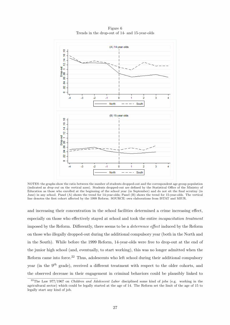
Figure 6Trends in the drop-out of 14- and 15-year-olds

NOTES: the graphs show the ratio between the number of students dropped-out and the correspondent age group population(indicated as drop-out on the vertical axes). Students dropped-out are defined by the Statistical Office of the Ministry ofEducation as those who enrolled at the beginning of the school year (in September) and do not sit the final scrutiny (inJune) in any school. Panel (A) shows the trend for 14-year-olds; Panel (B) shows the trend for 15-year-olds. The verticalline denotes the first cohort affected by the 1999 Reform. SOURCE: own elaborations from ISTAT and MIUR.

and increasing their concentration in the school facilities determined a crime increasing effect,

especially on those who effectively stayed at school and took the entire incapacitation treatment

imposed by the Reform. Differently, there seems to be a deterrence effect induced by the Reform

on those who illegally dropped-out during the additional compulsory year (both in the North and

in the South). While before the 1999 Reform, 14-year-olds were free to drop-out at the end of

the junior high school (and, eventually, to start working), this was no longer admitted when the

Reform came into force.22 Thus, adolescents who left school during their additional compulsory

year (in the 9th grade), received a different treatment with respect to the older cohorts, and

the observed decrease in their engagement in criminal behaviors could be plausibly linked to

22The Law 977/1967 on Children and Adolescent Labor disciplined some kind of jobs (e.g. working in theagricultural sector) which could be legally started at the age of 14. The Reform set the limit of the age of 15 tolegally start any kind of job.

27

their status of illegality determined by the introduction of the Reform, as a consequence of their

decision to drop-out. Finally, given that a larger fraction of students in the South (as compared

to the North of the country) dropped-out during the first year of implementation of the Reform,

this unintended effect of deterrence on the dropped-out was plausibly larger in the South.

6.3 The social interactions and the criminal network channels

Increasing the amount of time adolescents spend at school may have effects on their criminal

behavior which are ex ante undetermined, as they may strictly depend on the kind of peers they

are forced to interact with in the additional time they spend at school. If increasing the time

spent at school also increases the time an adolescent spends with bad peers, then the additional

time spent at school might have the unintended consequence of helping the individuals to create

criminal networks, or to get in contact more easily with organized criminal networks already

existent outside the school, or it might help to reduce the cost of coordination for committing

a crime with peers (Jacob and Lefgren, 2003). In this sense, additional time spent at school

could also contribute to create or accumulate a criminal capital (Bayer et al., 2009). In Table

7 (Panel A, column 9) we have already documented that the increasing effect on adolescent

offending rate in the South persists at older ages (i.e. 16 and 17). This can be interpreted as

an indirect evidence of an increased criminal capital for those who were forced to spend more

time at school. Italian Southern regions are also heavily influenced by the pervasive presence of

Mafia-type criminal organizations (Calderoni, 2011, Pinotti, 2014). In these areas, the presence

of criminal networks (inside and outside the school) could facilitate the engagement in criminal

behaviors of youths, increase the expected value of participating in criminal activities and reduce

its social costs (Damm and Dustmann, 2014). Criminal networks and criminal organizations offer

more opportunities to commit crimes, via social interactions mechanisms, but also they protect

their own affiliates, thus lowering the perceived probability of being caught by the police, and

guarantee a fixed amount of illegal rent which could be competitive with respect to the legal

labor market opportunities.

We identify areas where organized crime is more pervasive (and it is likely to heavily influence

everyday life and student behavior in the school and out of the school) on the basis of a simple

territorial rule such that we classify as Mafia regions all provinces located in the three regions

where mafia-type organizations were historically born and are still deeply rooted in the economic

and social networks, notably: Campania, Calabria and Sicily (Lupo, 1993, Pinotti, 2014). Then

we repeat our baseline analysis on the subsamples of provinces partitioned according to this

criterion. As a sensitivity check, we use as a second measure to identify areas where Mafia is

28

more pervasive, the Mafia Index taken from Calderoni (2011), which is a comprehensive measure

of the presence of organized crime in each province.

Figure 7Heterogeneous effects across macro-areas: focus on Mafia regions

NOTES: the graphs show the estimated coefficients and 95% confidence intervals of population weighted models on thesubsamples of provinces in the North-West, North-East, Center and South of Italy. Southern regions are divided intotwo groups: Mafia and non-Mafia regions. Mafia regions include the provinces in the Southern regions where Mafia-typeorganizations were historically born and developed (i.e. provinces in Campania, Calabria and Sicily); Non-Mafia regionsinclude the provinces in all the other Southern regions (Pinotti, 2014). Panel (A) shows results from the 2SLS model; Panel(B) from the crime reduced form model. SOURCE: own elaborations from ISTAT and MIUR.

Figure 7 plots the 2SLS and reduced form coefficients (i.e. the parameter θ1 of Eq. 1 and

β1 of Eq. 3, respectively), and the corresponding 95% confidence intervals, for the subsamples

of provinces defined as explained above. Figure 8 repeats the same exercise partitioning all

the provinces into the quartiles of the distribution of the Mafia Index. Focusing on Figure 7,

it can be noticed that while the crime reducing effect of education is prevalently associated to

the provinces in the North-West of the country, while the crime increasing effect is present in

Mafia-regions only.23

23In particular, the negative and statistically significant effects (both in the 2SLS and in reduced form models)arise from the two biggest regions in the North-West (Lombardy and Piedmont), while the positive and statisticallysignificant effects originate from two of the Mafia regions (Campania and Sicily). Detailed results are available

29

Figure 8Heterogeneous effects according to the Mafia Index

NOTES: the graphs show the estimated coefficients and 95% confidence intervals of population weighted models on thesubsamples of provinces in the four quartiles of the distribution of the Mafia Index (Calderoni, 2011). Panel (A) showsresults from the 2SLS model; Panel (B) from the crime reduced form model. SOURCE: own elaborations from ISTAT,MIUR and (Calderoni, 2011).

30

The increasing effects of education on juvenile crime documented in the literature are usually

linked to the differences in the types of offenses committed (Jacob and Lefgren, 2003, Luallen,

2006). To test whether the 1999 Reform had a differential impact on the types of crimes

in the South of the country, we take advantage of additional data which make it possible to

distinguish between violent, property and drug related crimes. A drawback of these data is

that, for confidentiality reasons, they allow to construct only region by year cells of the overall

offending rate of adolescents aged 14 to 17. Thus, while proving useful to our purposes, the

results must be interpreted with caution.24

Table 8Analysis by crime category

(1) (2) (3) (4) (5) (6)

Violent Property

Reform 0.18 0.08 0.10 -0.85 -1.45 -1.21(0.33) (0.35) (0.34) (0.85) (0.90) (0.77)

Reform * South 0.20 1.20*(0.26) (0.66)

Reform * Mafia regions 0.23 0.07(0.29) (0.69)

R. sq. 0.72 0.72 0.72 0.71 0.71 0.70N.Observations 178 178 178 178 178 178

Drug and economic related Total

Reform -0.65** -1.08*** -1.09*** -1.57 -2.82* -2.34(0.31) (0.32) (0.31) (1.36) (1.45) (1.42)

Reform * South 0.85*** 2.47**(0.24) (1.06)

Reform * Mafia regions 1.19*** 2.09*(0.26) (1.20)

R. sq. 0.53 0.56 0.58 0.64 0.65 0.65N.Observations 178 178 178 178 178 178

Region trends and year FE yes yes yes yes yes yesControl variables yes yes yes yes yes yes

NOTES: population weighted OLS estimated on region-year cells. The dependent variable of the 2SLS and reduced formmodels are the regional offending rates calculated for 14- to 17-year-olds. For the control variables included in the baselinespecification see Table 2. The specification also includes year fixed effects and regional linear trends. Robust standarderrors in parenthesis. Asterisks denote statistical significance at the * p < 0.1, ** p < 0.05, *** p < 0.01 levels.

We perform a reduced form analysis contrasting the adolescent offending rate before and

after the implementation of the Reform, estimating OLS regressions where we include year

fixed effects, regional-specific time trends, and the usual vector of time variant control variables

calculated at the regional level (Xjt).25

upon request.24Based on the regressions performed on 16- and 17-year-olds, we may expect these results to provide the lower

bound of the true effects, at least for the Northern provinces. We do not show the results for the residual category(Other crimes) as it does not display any statistically significant effect. They are available upon request.

25The sample of school years is the same used in the main analysis. Given that we cannot distinguish betweenthe adolescent aged 14 or 15, and given that in the school year 1999/00 the Reform only applied to 14-year-olds(and not to 15-year-olds), we drop the observations for this year.

31

In line with our baseline analysis, we do not find statistically significant effects overall.

To see whether a differential effect is present in the South, we interact the dummy Reform

with a dummy variable indicating the regions located in the South. First, the estimates on

the total offending rate confirm the findings in the main analysis: while the Reform has a

crime decreasing effect in the North, this effect is considerably mitigated in the South. Then,

while no statistically significant effects are found for violent crimes, drug and economic related

crimes decrease in the North more than in the South. Given that drug and economic related

crimes are especially sensitive to juvenile concentration and the creation and exploitation of

criminal networks (Damm and Gorinas, 2014), these findings are consistent with the idea that

the increase in the youth concentration and in the amount of time spent in school facilities,

increased adolescents interactions and widened their illegal market prospects for petty crimes,

such as smuggling and drug trafficking. Finally, in Table 8, columns 3 and 6, we also evaluate the

effects of the Reform on the different types of offenses focusing on Mafia regions, instead of on the

whole subsample of the Southern regions. The analysis confirms that the effects estimated for

the South prevalently originate from Mafia-related regions: the total offending rate significantly

increases in the Mafia regions as compared to the rest of the country, while drug and economic

related crimes significantly decrease in the rest of the country but marginally increase in the

Mafia regions.

7 Conclusions and policy implications

The causes of the territorial heterogeneity in the pattern of crime rates have long been debated

in the literature. Glaeser et al. (1996) show that only 30 percent of the patterns in crime rates

across areas are explained by observable area characteristics, and that social interactions may

play a substantive role in explaining such variations. Akomak and ter Weel (2012) show that

local institutions and social capital may explain an important part of the territorial variability

in crime rates. Concerning the causal relation between education and crime, only Luallen (2006)

finds that the incapacitation effect of school causes a statistically significant effects in the youth

crime rate in urban areas, while no effects are detected rural and sub-urban areas.

In this paper, we estimate the causal link between school attendance and adolescent offend-

ing rate, exploiting the implementation of a Reform, which has increased compulsory education

by one year. In our baseline analysis, by adopting a 2SLS estimation and by using the Reform

as an instrument, we find that a one percentage point increase in enrollment rate at high school

(grades 9 and 10) decreases the adolescent offending rate by 1.34 percent with respect to the

mean in the North of the country, while increasing it by almost 4 percent in the South. Edu-

32

cation might affect youth criminal behavior through several channels, which may play different

role across the territory and help to explain the observed regional divide. Extending the analysis

to the offending rates of older adolescents, we show that a human capital effect does not operate

in the short run. We find that the crime reducing effect of education uncovered in the North

of the country is mainly driven by the incapacitation channel, as typically shown in the recent

literature (Anderson, 2013, Bertheleon and Kruger, 2011). Conversely, the increase in the ado-

lescent offending rate observed in the South is consistent with a criminal capital accumulation

mechanism, mainly operating through the channels of the social interactions and the organized

criminal networks. Conducting the analysis by crime category also shows that drug and eco-

nomic related crimes are the more influenced by the increasing effect observed in the South,

consistently with the extension of the (illegal) market size for drug trafficking and smuggling

through an increased concentration of peers in the school facilities (Damm and Gorinas, 2014,

Jacob and Lefgren, 2003, Luallen, 2006).

Southern Italy is an area where Mafia-type criminal organizations deeply influence social

life and economic activities (Mete, 2009, Pinotti, 2014). Growing up and attending school in

such areas may have important effects on adolescent criminal behavior (Cederna, 2013, Damm

and Dustmann, 2014). Our results suggest that one additional year of schooling can have

different effects on adolescent offending rates depending on the quality of local institutions and

the pervasiveness of organized crime, so that spending additional time at school is not enough to

determine strong incapacitation effects in areas at risk. In fact, in these areas young criminals

might find illegal activities more easily and with higher reward and this seems to be even

exacerbated through the increase youth concentration in the school facilities which followed the

implementation of the Reform.

The evidence we present also points to the fact that keeping youths at school simply to

prevent them from staying on the street in areas characterized by pervasive organized crime is

not enough to ensure the same level of crime reduction as it could be reached in areas where

organized crime is not pervasive. Still, education policies should be aimed at stimulating a

role for the human capital effect to work, increasing the sense of civic duty and legality and

designing adequate school activities for students living in areas where illegal opportunities seem

more profitable than the legal activities. For example, Heller et al. (2013) analyze the effect of an

intervention targeted for disadvantaged male youth attending grades 7-10 in high-crime Chicago

neighborhoods. Interestingly, the intervention does not simply entail an increase of the time

spent at school; rather it was composed by a vast array of programs including regular interactions

with pro-social adults and in-school cognitive behavioral therapy.26 The authors show that

26Cognitive behavioral therapy (CBT) is psychological treatment designed to reduce common judgment and

33

program participation reduced violent-crime arrests during the program year 44 percent, a crime

reducing effect that more than doubles what the existing literature on the incapacitation effect

of schooling has generally found.

Further research is thus needed in order to disentangle the separate contribution of the inca-

pacitation and social interactions channels in determining their effects on adolescent crime, and

to understand how these channels might interact with the existing criminal networks and social

institutions. Indeed, a deeper understanding of these mechanisms might also be particularly

useful to design optimal behavioral policy interventions to counter adolescent crime.

decision-making problems related to automatic behavior and biased beliefs.

34

References

Akomak, S. I. and B. ter Weel (2012). The impact of social capital on crime: Evidence from the

Netherlands. Regional Science and Urban Economics 42 (2012), 323–340.

Anderson, M. D. (2013). In school and out of trouble? The minimum drop out age and juvenile

crime. The Review of Economics and Statistics forthcoming, doi: 10.1162/RESTa00360.

Anderson, M. D., B. Hansen, and M. B. Walker (2013). The minimum dropout age and student

victimization. Economics of Education Review 35, 66–74.

Barone, G. and S. Mocetti (2014). Natural disasters, growth and institutions: A tale of two

earthquakes. Journal of Urban Economics 84, 52–66.

Bayer, P., R. Hjalmarsson, and D. Pozen (2009). Building criminal capital behind bars: Peer

effects in juvenile corrections. The Quarterly Journal of Economics.

Benadusi, L. and O. Niceforo (2010). Obbligo scolastico o di istruzione: alla ricerca dell’equita.

FGA Working Paper No. 27/2010 .

Bertheleon, M. E. and D. I. Kruger (2011). Risky behavior among youth: Incapacitation effects

of school on adolescent motherhood and crime in Chile. Journal of Public Economics 95,

41–53.

Bianchi, M., P. Buonanno, and P. Pinotti (2012). Do immigrants cause crime? Journal of the

European Economic Association 10 (6), 1318–1347.

Calderoni, F. (2011). Where is the Mafia in Italy? Measuring the presence of the Mafia across

Italian provinces. Global Crime 12 (1), 41–69.

Card, D. and L. Giuliano (2013). Peer effects and multiple equilibria in the risky behavior of

friends. The Review of Economics and Statistics 95 (4), 1130–1149.

Cederna, G. (2013). Atlante dell’infanzia a rischio. Technical report, Save the Children, Italy.

Cohen, M. and A. Piquero (2009). New evidence on the monetary value of saving a high risk

youth. Journal of Quantitative Criminology 25 (1), 25–49.

Damm, A. P. and C. Dustmann (2014). Does growing up in a high crime neighborhood affect

youth criminal behavior? American Economic Review 104, 1806–1832.

Damm, A. P. and C. Gorinas (2014). Deal drugs once, deal drugs twice: Peer effects on recidivism

from prisonsl. Aahrus Unversity mimeo.

35

Dipartimento di Giustizia Minorile (2007). Minorenni denunciati alle Procure della Repubblica

presso i Tribunali per i Minorenni. Technical report, Dipartimento Giustizia Minorile, Rome.

Fougere, D., F. Kramarz, and J. Pouget (2009). Youth unemployment and crime in France.

Journal of the European Economic Association 7 (5), 909–938.

Glaeser, E., B. Sacerdote, and J. A.Scheinkman (1996). Crime and social interactions. The

Quarterly Journal of Economics 111(2), 507–548.

Guiso, L., P. Sapienza, and L. Zingales (2013). Long-term persistence. EIEF Working Paper

No. 23/2013 . Einaudi Institute Economics and Finance, Rome.

Heller, S., H. A. Pollack, R. Ander, and J. Ludwing (2013). Preventing youth violence and

dropout: a randomized field experiment. NBER Working Paper No. 19014 . National Bureau

of Economic Research.

Hjalmarsson, R. and L. Lochner (2012). The impact of education on crime: international

evidence. CEsifo DICE Report 2/2012 , 49–55.

Jacob, B. and L. Lefgren (2003). Are idle hands the devil’s workshop? Incapacitation, concen-

tration, and juvenile crime. American Economic Review 93, 1560–1577.

Lochner, L. (2011). Nonproduction benefits of education: Crime, health, and good citizenship.

In E. A. Hanushek, S. Machin, and L. Woessmann (Eds.), Handbook of The Economics of

Education. Elsevier Science B.V.

Lochner, L. and E. Moretti (2004). The effect of education on crime: Evidence from prison

inmates, arrests, and self-reports. American Economic Review 94(1), 155–189.

Luallen, J. (2006). School’s out...forever: a study of juvenile crime, at risk youths and teachers

strikes. Journal of Urban Economics 59, 75–103.

Lupo, S. (1993). Storia della Mafia: dalle origini ai giorni nostri (1 ed.). Roma: Donzelli.

Machin, S., O. Marie, and S. Vujic (2011). The crime reducing effect of education. The Economic

Journal 121 (May), 463–484.

Mete, V. (2009). Fuori dal comune. Lo scioglimento delle amministrazioni locali per infiltrazioni

mafiose (1 ed.). Roma: Bonanno.

Nagin, D. S. and K. Land (1993). Age, criminal careers, and population heterogeneity: Specifi-

cation and estimation of a nonparametric, mixed poisson model. Criminology 31(3), 327–362.

36

Osgood, W. (2000). Poisson-based regression analysis of aggregate crime rates. Journal of

Quantitative Criminology 16 (1), 21–43.

Oster, A. and J. Agell (2007). Crime and unemployment in turbolent times. Journal of the

European Economic Association 5 (4), 752–775.

Paccagnella, M. and P. Sestito (2014). School cheating and social capital. Bank of Italy Working

Paper No. 952/2014 .

Patacchini, E. and Y. Zenou (2009). Juvenile delinquency and conformism. The Journal of Law,

Economics, Organization 28(1), 1–31.

Pinotti, P. (2014). The economic costs of organized crime: evidence from Southern Italy. The

Economic Journal . forthcoming.

Stock, J. H. and M. Yogo (2005). Testing for weak instruments in linear IV regression. In

D. Andrews (Ed.), Identification and Inference for Econometric Models, pp. 80–108. New

York: Cambridge University Press.

UN (2003). Juvenile delinquency. Technical report, United Nations, New York.

37

A Juvenile delinquency in selected countries

Table A.1Characteristics of juvenile delinquency in selected countries

Suspected Prosecuted Incarcerated Incarceration rate

Juvenile Adult Juvenile Adult Juvenile Adult Juvenile Adult

Italy 53.03 1,228.75 32.89 906.62 1.6 100.82 3.03 8.20US 457.33 2,565.14Canada 265.65 1,666.35 174.37 1,156.30 6.91 99.54 2.60 5.97Spain 55.25 620.91Germany 344.15 2,329.71 93.01 814.02England and Wales 246.6 3,275.72 4.35 122.41Denmark 136.77 907.06 0.37 74.23 0.27 8.18Sweden 281.31 890.3 158.43 3.4 81.57 1.21 9.16Greece 26.96 1,847.87 0.73 88.2 2.71 4.77Japan 96.73 205.82 1.23 140.86 0.05 61.76 0.05 30.01Portugal 44.79 2,025.08 111.61 862.52 5.02 117.4 11.22 5.80

NOTES: figures are expressed as rates per 100,000 of total population. Suspected individuals are defined as persons broughtinto formal contact with the criminal justice system, regardless of the type of crime (where formal contact might includebeing suspected, arrested, cautioned); Incarcerated individuals are defined as persons held in prisons, penal institutionsor correctional institutions (including institutions for pretrial detention), regardless of the type of crime, in a selecteddate (June, 30); Incarceration rate is obtained as the percentage of incarcerated individuals over the total number ofsuspected individuals. Juveniles are defined as individuals under the age of 18 in all the selected countries except: Sweden(under 21), Portugal (under 20), Japan (under 19). SOURCE: United Nations Survey of Crime Trends and Operationsof Criminal Justice Systems (UN-CTS), United Nations Office for Drugs and Crime (UNODOC) (available at https:

//www.unodc.org/unodc/en/data-and-analysis/statistics/historic-data.html).

38

(*) Requests for copies should be sent to: Banca d’Italia – Servizio Struttura economica e finanziaria – Divisione Biblioteca e Archivio storico – Via Nazionale, 91 – 00184 Rome – (fax 0039 06 47922059). They are available on the Internet www.bancaditalia.it.

RECENTLY PUBLISHED “TEMI” (*)

N. 985 – Dif-in-dif estimators of multiplicative treatment effects, by Emanuele Ciani and Paul Fisher (October 2014).

N. 986 – An estimated DSGE model with search and matching frictions in the credit market, by Danilo Liberati (October 2014).

N. 987 – Large banks, loan rate markup and monetary policy, by Vincenzo Cuciniello and Federico M. Signoretti (October 2014).

N. 988 – The interest-rate sensitivity of the demand for sovereign debt. Evidence from OECD countries (1995-2011), by Giuseppe Grande, Sergio Masciantonio and Andrea Tiseno (October 2014).

N. 989 – The determinants of household debt: a cross-country analysis, by Massimo Coletta, Riccardo De Bonis and Stefano Piermattei (October 2014).

N. 990 – How much of bank credit risk is sovereign risk? Evidence from the Eurozone, by Junye Li and Gabriele Zinna (October 2014).

N. 991 – The scapegoat theory of exchange rates: the first tests, by Marcel Fratzscher, Dagfinn Rime, Lucio Sarno and Gabriele Zinna (October 2014).

N. 992 – Informed trading and stock market efficiency, by Taneli Mäkinen (October 2014).

N. 993 – Optimal monetary policy rules and house prices: the role of financial frictions, by Alessandro Notarpietro and Stefano Siviero (October 2014).

N. 994 – Trade liberalizations and domestic suppliers: evidence from Chile, by Andrea Linarello (November 2014).

N. 995 – Dynasties in professions: the role of rents, by Sauro Mocetti (November 2014).

N. 996 – Current account “core-periphery dualism” in the EMU, by Tatiana Cesaroni and Roberta De Santis (November 2014).

N. 997 – Macroeconomic effects of simultaneous implementation of reforms after the crisis, by Andrea Gerali, Alessandro Notarpietro and Massimiliano Pisani (November 2014).

N. 998 – Changing labour market opportunities for young people in Italy and the role of the family of origin, by Gabriella Berloffa, Francesca Modena and Paola Villa (January 2015).

N. 999 – Looking behind mortgage delinquencies, by Sauro Mocetti and Eliana Viviano (January 2015).

N. 1000 – Sectoral differences in managers’ compensation: insights from a matching model, by Emanuela Ciapanna, Marco Taboga and Eliana Viviano (January 2015).

N. 1001 – How does foreign demand activate domestic value added? A comparison among the largest euro-area economies, by Rita Cappariello and Alberto Felettigh (January 2015).

N. 1002 – Structural reforms and zero lower bound in a monetary union, by Andrea Gerali, Alessandro Notarpietro and Massimiliano Pisani (January 2015).

N. 1003 – You’ve come a long way, baby. Effects of commuting times on couples’ labour supply, by Francesca Carta and Marta De Philippis (March 2015).

N. 1004 – Ownership networks and aggregate volatility, by Lorenzo Burlon (March 2015).

N. 1005 – Strategy and tactics in public debt manamgement, by Davide Dottori and Michele Manna (March 2015).

N. 1006 – Inward foreign direct investment and innovation: evidence from Italian provinces, by Roberto Antonietti, Raffaello Bronzini and Giulio Cainelli (March 2015).

N. 1007 – The macroeconomic effects of the sovereign debt crisis in the euro area, by Stefano Neri and Tiziano Ropele (March 2015).

"TEMI" LATER PUBLISHED ELSEWHERE

2012

F. CINGANO and A. ROSOLIA, People I know: job search and social networks, Journal of Labor Economics, v. 30, 2, pp. 291-332, TD No. 600 (September 2006).

G. GOBBI and R. ZIZZA, Does the underground economy hold back financial deepening? Evidence from the italian credit market, Economia Marche, Review of Regional Studies, v. 31, 1, pp. 1-29, TD No. 646 (November 2006).

S. MOCETTI, Educational choices and the selection process before and after compulsory school, Education Economics, v. 20, 2, pp. 189-209, TD No. 691 (September 2008).

P. PINOTTI, M. BIANCHI and P. BUONANNO, Do immigrants cause crime?, Journal of the European Economic Association , v. 10, 6, pp. 1318–1347, TD No. 698 (December 2008).

M. PERICOLI and M. TABOGA, Bond risk premia, macroeconomic fundamentals and the exchange rate, International Review of Economics and Finance, v. 22, 1, pp. 42-65, TD No. 699 (January 2009).

F. LIPPI and A. NOBILI, Oil and the macroeconomy: a quantitative structural analysis, Journal of European Economic Association, v. 10, 5, pp. 1059-1083, TD No. 704 (March 2009).

G. ASCARI and T. ROPELE, Disinflation in a DSGE perspective: sacrifice ratio or welfare gain ratio?, Journal of Economic Dynamics and Control, v. 36, 2, pp. 169-182, TD No. 736 (January 2010).

S. FEDERICO, Headquarter intensity and the choice between outsourcing versus integration at home or abroad, Industrial and Corporate Chang, v. 21, 6, pp. 1337-1358, TD No. 742 (February 2010).

I. BUONO and G. LALANNE, The effect of the Uruguay Round on the intensive and extensive margins of trade, Journal of International Economics, v. 86, 2, pp. 269-283, TD No. 743 (February 2010).

A. BRANDOLINI, S. MAGRI and T. M SMEEDING, Asset-based measurement of poverty, In D. J. Besharov and K. A. Couch (eds), Counting the Poor: New Thinking About European Poverty Measures and Lessons for the United States, Oxford and New York: Oxford University Press, TD No. 755 (March 2010).

S. GOMES, P. JACQUINOT and M. PISANI, The EAGLE. A model for policy analysis of macroeconomic interdependence in the euro area, Economic Modelling, v. 29, 5, pp. 1686-1714, TD No. 770 (July 2010).

A. ACCETTURO and G. DE BLASIO, Policies for local development: an evaluation of Italy’s “Patti Territoriali”, Regional Science and Urban Economics, v. 42, 1-2, pp. 15-26, TD No. 789 (January 2006).

E. COCOZZA and P. PISELLI, Testing for east-west contagion in the European banking sector during the financial crisis, in R. Matoušek; D. Stavárek (eds.), Financial Integration in the European Union, Taylor & Francis, TD No. 790 (February 2011).

F. BUSETTI and S. DI SANZO, Bootstrap LR tests of stationarity, common trends and cointegration, Journal of Statistical Computation and Simulation, v. 82, 9, pp. 1343-1355, TD No. 799 (March 2006).

S. NERI and T. ROPELE, Imperfect information, real-time data and monetary policy in the Euro area, The Economic Journal, v. 122, 561, pp. 651-674, TD No. 802 (March 2011).

A. ANZUINI and F. FORNARI, Macroeconomic determinants of carry trade activity, Review of International Economics, v. 20, 3, pp. 468-488, TD No. 817 (September 2011).

M. AFFINITO, Do interbank customer relationships exist? And how did they function in the crisis? Learning from Italy, Journal of Banking and Finance, v. 36, 12, pp. 3163-3184, TD No. 826 (October 2011).

P. GUERRIERI and F. VERGARA CAFFARELLI, Trade Openness and International Fragmentation of Production in the European Union: The New Divide?, Review of International Economics, v. 20, 3, pp. 535-551, TD No. 855 (February 2012).

V. DI GIACINTO, G. MICUCCI and P. MONTANARO, Network effects of public transposrt infrastructure: evidence on Italian regions, Papers in Regional Science, v. 91, 3, pp. 515-541, TD No. 869 (July 2012).

A. FILIPPIN and M. PACCAGNELLA, Family background, self-confidence and economic outcomes, Economics of Education Review, v. 31, 5, pp. 824-834, TD No. 875 (July 2012).

2013

A. MERCATANTI, A likelihood-based analysis for relaxing the exclusion restriction in randomized

experiments with imperfect compliance, Australian and New Zealand Journal of Statistics, v. 55, 2, pp. 129-153, TD No. 683 (August 2008).

F. CINGANO and P. PINOTTI, Politicians at work. The private returns and social costs of political connections, Journal of the European Economic Association, v. 11, 2, pp. 433-465, TD No. 709 (May 2009).

F. BUSETTI and J. MARCUCCI, Comparing forecast accuracy: a Monte Carlo investigation, International Journal of Forecasting, v. 29, 1, pp. 13-27, TD No. 723 (September 2009).

D. DOTTORI, S. I-LING and F. ESTEVAN, Reshaping the schooling system: The role of immigration, Journal of Economic Theory, v. 148, 5, pp. 2124-2149, TD No. 726 (October 2009).

A. FINICELLI, P. PAGANO and M. SBRACIA, Ricardian Selection, Journal of International Economics, v. 89, 1, pp. 96-109, TD No. 728 (October 2009).

L. MONTEFORTE and G. MORETTI, Real-time forecasts of inflation: the role of financial variables, Journal of Forecasting, v. 32, 1, pp. 51-61, TD No. 767 (July 2010).

R. GIORDANO and P. TOMMASINO, Public-sector efficiency and political culture, FinanzArchiv, v. 69, 3, pp. 289-316, TD No. 786 (January 2011).

E. GAIOTTI, Credit availablility and investment: lessons from the "Great Recession", European Economic Review, v. 59, pp. 212-227, TD No. 793 (February 2011).

F. NUCCI and M. RIGGI, Performance pay and changes in U.S. labor market dynamics, Journal of Economic Dynamics and Control, v. 37, 12, pp. 2796-2813, TD No. 800 (March 2011).

G. CAPPELLETTI, G. GUAZZAROTTI and P. TOMMASINO, What determines annuity demand at retirement?, The Geneva Papers on Risk and Insurance – Issues and Practice, pp. 1-26, TD No. 805 (April 2011).

A. ACCETTURO e L. INFANTE, Skills or Culture? An analysis of the decision to work by immigrant women in Italy, IZA Journal of Migration, v. 2, 2, pp. 1-21, TD No. 815 (July 2011).

A. DE SOCIO, Squeezing liquidity in a “lemons market” or asking liquidity “on tap”, Journal of Banking and Finance, v. 27, 5, pp. 1340-1358, TD No. 819 (September 2011).

S. GOMES, P. JACQUINOT, M. MOHR and M. PISANI, Structural reforms and macroeconomic performance in the euro area countries: a model-based assessment, International Finance, v. 16, 1, pp. 23-44, TD No. 830 (October 2011).

G. BARONE and G. DE BLASIO, Electoral rules and voter turnout, International Review of Law and Economics, v. 36, 1, pp. 25-35, TD No. 833 (November 2011).

O. BLANCHARD and M. RIGGI, Why are the 2000s so different from the 1970s? A structural interpretation of changes in the macroeconomic effects of oil prices, Journal of the European Economic Association, v. 11, 5, pp. 1032-1052, TD No. 835 (November 2011).

R. CRISTADORO and D. MARCONI, Household savings in China, in G. Gomel, D. Marconi, I. Musu, B. Quintieri (eds), The Chinese Economy: Recent Trends and Policy Issues, Springer-Verlag, Berlin, TD No. 838 (November 2011).

A. ANZUINI, M. J. LOMBARDI and P. PAGANO, The impact of monetary policy shocks on commodity prices, International Journal of Central Banking, v. 9, 3, pp. 119-144, TD No. 851 (February 2012).

R. GAMBACORTA and M. IANNARIO, Measuring job satisfaction with CUB models, Labour, v. 27, 2, pp. 198-224, TD No. 852 (February 2012).

G. ASCARI and T. ROPELE, Disinflation effects in a medium-scale new keynesian model: money supply rule versus interest rate rule, European Economic Review, v. 61, pp. 77-100, TD No. 867 (April 2012).

E. BERETTA and S. DEL PRETE, Banking consolidation and bank-firm credit relationships: the role of geographical features and relationship characteristics, Review of Economics and Institutions, v. 4, 3, pp. 1-46, TD No. 901 (February 2013).

M. ANDINI, G. DE BLASIO, G. DURANTON and W. STRANGE, Marshallian labor market pooling: evidence from Italy, Regional Science and Urban Economics, v. 43, 6, pp.1008-1022, TD No. 922 (July 2013).

G. SBRANA and A. SILVESTRINI, Forecasting aggregate demand: analytical comparison of top-down and bottom-up approaches in a multivariate exponential smoothing framework, International Journal of Production Economics, v. 146, 1, pp. 185-98, TD No. 929 (September 2013).

A. FILIPPIN, C. V, FIORIO and E. VIVIANO, The effect of tax enforcement on tax morale, European Journal of Political Economy, v. 32, pp. 320-331, TD No. 937 (October 2013).

2014

G. M. TOMAT, Revisiting poverty and welfare dominance, Economia pubblica, v. 44, 2, 125-149, TD No. 651

(December 2007).

M. TABOGA, The riskiness of corporate bonds, Journal of Money, Credit and Banking, v.46, 4, pp. 693-713, TD No. 730 (October 2009).

G. MICUCCI and P. ROSSI, Il ruolo delle tecnologie di prestito nella ristrutturazione dei debiti delle imprese in crisi, in A. Zazzaro (a cura di), Le banche e il credito alle imprese durante la crisi, Bologna, Il Mulino, TD No. 763 (June 2010).

F. D’AMURI, Gli effetti della legge 133/2008 sulle assenze per malattia nel settore pubblico, Rivista di politica economica, v. 105, 1, pp. 301-321, TD No. 787 (January 2011).

R. BRONZINI and E. IACHINI, Are incentives for R&D effective? Evidence from a regression discontinuity approach, American Economic Journal : Economic Policy, v. 6, 4, pp. 100-134, TD No. 791 (February 2011).

P. ANGELINI, S. NERI and F. PANETTA, The interaction between capital requirements and monetary policy, Journal of Money, Credit and Banking, v. 46, 6, pp. 1073-1112, TD No. 801 (March 2011).

M. BRAGA, M. PACCAGNELLA and M. PELLIZZARI, Evaluating students’ evaluations of professors, Economics of Education Review, v. 41, pp. 71-88, TD No. 825 (October 2011).

M. FRANCESE and R. MARZIA, Is there Room for containing healthcare costs? An analysis of regional spending differentials in Italy, The European Journal of Health Economics, v. 15, 2, pp. 117-132, TD No. 828 (October 2011).

L. GAMBACORTA and P. E. MISTRULLI, Bank heterogeneity and interest rate setting: what lessons have we learned since Lehman Brothers?, Journal of Money, Credit and Banking, v. 46, 4, pp. 753-778, TD No. 829 (October 2011).

M. PERICOLI, Real term structure and inflation compensation in the euro area, International Journal of Central Banking, v. 10, 1, pp. 1-42, TD No. 841 (January 2012).

E. GENNARI and G. MESSINA, How sticky are local expenditures in Italy? Assessing the relevance of the flypaper effect through municipal data, International Tax and Public Finance, v. 21, 2, pp. 324-344, TD No. 844 (January 2012).

V. DI GACINTO, M. GOMELLINI, G. MICUCCI and M. PAGNINI, Mapping local productivity advantages in Italy: industrial districts, cities or both?, Journal of Economic Geography, v. 14, pp. 365–394, TD No. 850 (January 2012).

A. ACCETTURO, F. MANARESI, S. MOCETTI and E. OLIVIERI, Don't Stand so close to me: the urban impact of immigration, Regional Science and Urban Economics, v. 45, pp. 45-56, TD No. 866 (April 2012).

M. PORQUEDDU and F. VENDITTI, Do food commodity prices have asymmetric effects on euro area inflation, Studies in Nonlinear Dynamics and Econometrics, v. 18, 4, pp. 419-443, TD No. 878 (September 2012).

S. FEDERICO, Industry dynamics and competition from low-wage countries: evidence on Italy, Oxford Bulletin of Economics and Statistics, v. 76, 3, pp. 389-410, TD No. 879 (September 2012).

F. D’AMURI and G. PERI, Immigration, jobs and employment protection: evidence from Europe before and during the Great Recession, Journal of the European Economic Association, v. 12, 2, pp. 432-464, TD No. 886 (October 2012).

M. TABOGA, What is a prime bank? A euribor-OIS spread perspective, International Finance, v. 17, 1, pp. 51-75, TD No. 895 (January 2013).

L. GAMBACORTA and F. M. SIGNORETTI, Should monetary policy lean against the wind? An analysis based on a DSGE model with banking, Journal of Economic Dynamics and Control, v. 43, pp. 146-74, TD No. 921 (July 2013).

M. BARIGOZZI, CONTI A.M. and M. LUCIANI, Do euro area countries respond asymmetrically to the common monetary policy?, Oxford Bulletin of Economics and Statistics, v. 76, 5, pp. 693-714, TD No. 923 (July 2013).

U. ALBERTAZZI and M. BOTTERO, Foreign bank lending: evidence from the global financial crisis, Journal of International Economics, v. 92, 1, pp. 22-35, TD No. 926 (July 2013).

R. DE BONIS and A. SILVESTRINI, The Italian financial cycle: 1861-2011, Cliometrica, v.8, 3, pp. 301-334, TD No. 936 (October 2013).

D. PIANESELLI and A. ZAGHINI, The cost of firms’ debt financing and the global financial crisis, Finance Research Letters, v. 11, 2, pp. 74-83, TD No. 950 (February 2014).

A. ZAGHINI, Bank bonds: size, systemic relevance and the sovereign, International Finance, v. 17, 2, pp. 161-183, TD No. 966 (July 2014).

M. SILVIA, Does issuing equity help R&D activity? Evidence from unlisted Italian high-tech manufacturing firms, Economics of Innovation and New Technology, v. 23, 8, pp. 825-854, TD No. 978 (October 2014).

G. BARONE and S. MOCETTI, Natural disasters, growth and institutions: a tale of two earthquakes, Journal of Urban Economics, v. 84, pp. 52-66, TD No. 949 (January 2014).

2015

G. BULLIGAN, M. MARCELLINO and F. VENDITTI, Forecasting economic activity with targeted predictors,

International Journal of Forecasting, v. 31, 1, pp. 188-206, TD No. 847 (February 2012).

A. CIARLONE, House price cycles in emerging economies, Studies in Economics and Finance, v. 32, 1, TD No. 863 (May 2012).

G. BARONE and G. NARCISO, Organized crime and business subsidies: Where does the money go?, Journal of Urban Economics, v. 86, pp. 98-110, TD No. 916 (June 2013).

P. ALESSANDRI and B. NELSON, Simple banking: profitability and the yield curve, Journal of Money, Credit and Banking, v. 47, 1, pp. 143-175, TD No. 945 (January 2014).

R. AABERGE and A. BRANDOLINI, Multidimensional poverty and inequality, in A. B. Atkinson and F. Bourguignon (eds.), Handbook of Income Distribution, Volume 2A, Amsterdam, Elsevier, TD No. 976 (October 2014).

M. FRATZSCHER, D. RIMEC, L. SARNOB and G. ZINNA, The scapegoat theory of exchange rates: the first tests, Journal of Monetary Economics, v. 70, 1, pp. 1-21, TD No. 991 (November 2014).

FORTHCOMING

M. BUGAMELLI, S. FABIANI and E. SETTE, The age of the dragon: the effect of imports from China on firm-level prices, Journal of Money, Credit and Banking, TD No. 737 (January 2010).

G. DE BLASIO, D. FANTINO and G. PELLEGRINI, Evaluating the impact of innovation incentives: evidence from an unexpected shortage of funds, Industrial and Corporate Change, TD No. 792 (February 2011).

A. DI CESARE, A. P. STORK and C. DE VRIES, Risk measures for autocorrelated hedge fund returns, Journal of Financial Econometrics, TD No. 831 (October 2011).

D. FANTINO, A. MORI and D. SCALISE, Collaboration between firms and universities in Italy: the role of a firm's proximity to top-rated departments, Rivista Italiana degli economisti, TD No. 884 (October 2012).

M. MARCELLINO, M. PORQUEDDU and F. VENDITTI, Short-Term GDP Forecasting with a mixed frequency dynamic factor model with stochastic volatility, Journal of Business & Economic Statistics, TD No. 896 (January 2013).

M. ANDINI and G. DE BLASIO, Local development that money cannot buy: Italy’s Contratti di Programma, Journal of Economic Geography, TD No. 915 (June 2013).

J. LI and G. ZINNA, On bank credit risk: sytemic or bank-specific? Evidence from the US and UK, Journal of Financial and Quantitative Analysis, TD No. 951 (February 2015).