temi di discussione - banca d'italia · temi di discussione (working papers) evidence on the...
TRANSCRIPT

Temi di Discussione(Working Papers)
Evidence on the impact of R&D and ICT investment on innovation and productivity in Italian firms
by Bronwyn H. Hall, Francesca Lotti and Jacques Mairesse
Num
ber 874Ju
ly 2
012


Temi di discussione(Working papers)
Evidence on the impact of R&D and ICT investment on innovation and productivity in Italian firms
by Bronwyn H. Hall, Francesca Lotti and Jacques Mairesse
Number 874 - July 2012

The purpose of the Temi di discussione series is to promote the circulation of workingpapers prepared within the Bank of Italy or presented in Bank seminars by outside economists with the aim of stimulating comments and suggestions.
The views expressed in the articles are those of the authors and do not involve the responsibility of the Bank.
Editorial Board: Silvia Magri, Massimo Sbracia, Luisa Carpinelli, Emanuela Ciapanna, Francesco D’Amuri, Alessandro Notarpietro, Pietro Rizza, Concetta Rondinelli, Tiziano Ropele, Andrea Silvestrini, Giordano Zevi.Editorial Assistants: Roberto Marano, Nicoletta Olivanti.

EVIDENCE ON THE IMPACT OF R&D AND ICT INVESTMENT ON INNOVATION AND PRODUCTIVITY IN ITALIAN FIRMS
by Bronwyn H. Hall,# Francesca Lotti,§ and Jacques Mairesse
Abstract
The paper investigates R&D and ICT investment at firm level, assessing their relative importance and the extent to which they are complements or substitutes. We use data on a large unbalanced panel sample from four consecutive waves of a survey of Italian manufacturing firms, together with a version of the model developed by Crepon et al., 1998, modified to include ICT investment and R&D as the two main inputs of innovation and productivity. We find that R&D and ICT are both strongly associated with innovation and productivity, with R&D being more important for innovation and ICT for productivity. We explore their possible complementarity in innovation and production but find none, although there is complementarity between R&D and worker skill in innovation.
JEL Classification: L60, O31, O33. Keywords: R&D, ICT, innovation, productivity, complementarity, Italy.
Contents
1. Introduction................................................................................................................ 5 2. ICT and productivity: a micro perspective ................................................................ 7 3. The extended CDM model ....................................................................................... 10 4. Data and descriptive statistics .................................................................................. 14 5. Results and discussion ............................................................................................. 15 6. ICT and R&D: complements or substitutes? ........................................................... 23 7. Conclusions.............................................................................................................. 24 References...................................................................................................................... 26 Appendix........................................................................................................................ 28 Tables and figures .......................................................................................................... 30
# University of California at Berkeley, Maastricht University, NBER, and IFS. § Bank of Italy, Economic Research and International Relations. CREST (ENSAE, Paris), UNU-MERIT (Maastricht University), and NBER.

5
1. Introduction*
Both Research and Development (R&D) and Information and Communication
Technology (ICT) investment have been identified as areas of relative
underperformance in Europe vis-à-vis the United States. For example, Van Ark et al.
(2003) concluded the following in their study of the reasons for lower productivity
growth in Europe: “The results show that U.S. productivity has grown faster than in the
EU because of a larger employment share in the ICT producing sector and faster
productivity growth in services industries that make intensive use of ICT.” Moncada-
Paternò-Castello et al. (2009), Hall and Mairesse (2009), and O’Sullivan (2006) all
point to the differences in industrial structure, specifically the smaller ICT producing
sector as the main cause of lower R&D intensity in Europe.
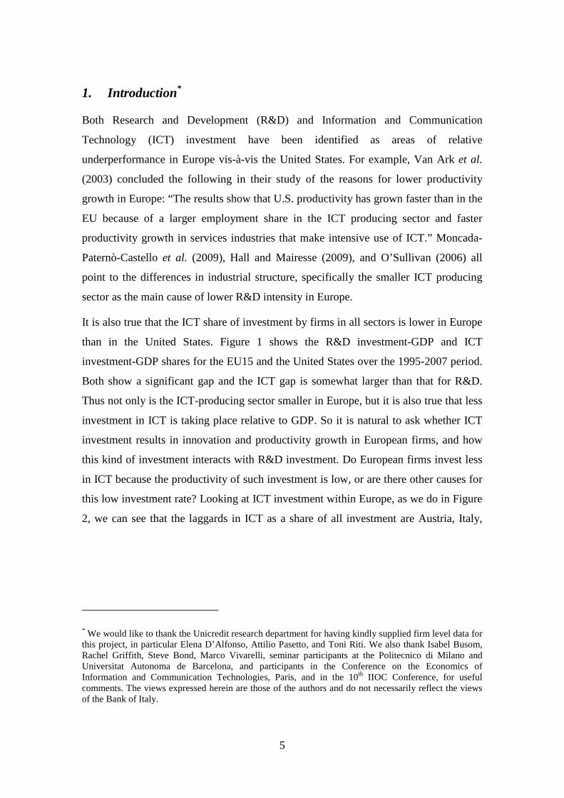
It is also true that the ICT share of investment by firms in all sectors is lower in Europe
than in the United States. Figure 1 shows the R&D investment-GDP and ICT
investment-GDP shares for the EU15 and the United States over the 1995-2007 period.
Both show a significant gap and the ICT gap is somewhat larger than that for R&D.
Thus not only is the ICT-producing sector smaller in Europe, but it is also true that less
investment in ICT is taking place relative to GDP. So it is natural to ask whether ICT
investment results in innovation and productivity growth in European firms, and how
this kind of investment interacts with R&D investment. Do European firms invest less
in ICT because the productivity of such investment is low, or are there other causes for
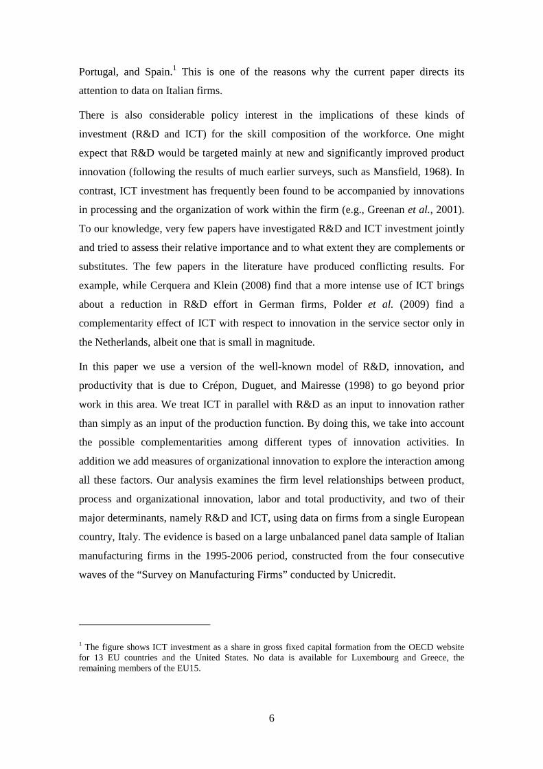
this low investment rate? Looking at ICT investment within Europe, as we do in Figure
2, we can see that the laggards in ICT as a share of all investment are Austria, Italy,
* We would like to thank the Unicredit research department for having kindly supplied firm level data for this project, in particular Elena D’Alfonso, Attilio Pasetto, and Toni Riti. We also thank Isabel Busom, Rachel Griffith, Steve Bond, Marco Vivarelli, seminar participants at the Politecnico di Milano and Universitat Autonoma de Barcelona, and participants in the Conference on the Economics of Information and Communication Technologies, Paris, and in the 10th IIOC Conference, for useful comments. The views expressed herein are those of the authors and do not necessarily reflect the views of the Bank of Italy.
6
Portugal, and Spain.1 This is one of the reasons why the current paper directs its
attention to data on Italian firms.
There is also considerable policy interest in the implications of these kinds of
investment (R&D and ICT) for the skill composition of the workforce. One might
expect that R&D would be targeted mainly at new and significantly improved product
innovation (following the results of much earlier surveys, such as Mansfield, 1968). In
contrast, ICT investment has frequently been found to be accompanied by innovations
in processing and the organization of work within the firm (e.g., Greenan et al., 2001).
To our knowledge, very few papers have investigated R&D and ICT investment jointly
and tried to assess their relative importance and to what extent they are complements or
substitutes. The few papers in the literature have produced conflicting results. For
example, while Cerquera and Klein (2008) find that a more intense use of ICT brings
about a reduction in R&D effort in German firms, Polder et al. (2009) find a
complementarity effect of ICT with respect to innovation in the service sector only in
the Netherlands, albeit one that is small in magnitude.
In this paper we use a version of the well-known model of R&D, innovation, and
productivity that is due to Crépon, Duguet, and Mairesse (1998) to go beyond prior
work in this area. We treat ICT in parallel with R&D as an input to innovation rather
than simply as an input of the production function. By doing this, we take into account
the possible complementarities among different types of innovation activities. In
addition we add measures of organizational innovation to explore the interaction among
all these factors. Our analysis examines the firm level relationships between product,
process and organizational innovation, labor and total productivity, and two of their
major determinants, namely R&D and ICT, using data on firms from a single European
country, Italy. The evidence is based on a large unbalanced panel data sample of Italian
manufacturing firms in the 1995-2006 period, constructed from the four consecutive
waves of the “Survey on Manufacturing Firms” conducted by Unicredit.
1 The figure shows ICT investment as a share in gross fixed capital formation from the OECD website for 13 EU countries and the United States. No data is available for Luxembourg and Greece, the remaining members of the EU15.

7
Taking advantage of our previous work (Hall, Lotti and Mairesse 2008 and 2009), and
in the spirit of Polder et al. (2009), we rely on an extension of a modified version of the
CDM model (Griffith et al., 2006) that includes ICT investment together with R&D as
two main inputs into innovation and productivity. This extension of the model
specification leads to augmented difficulties in estimation owing to the increased
number of equations with qualitative dependent variables: we bypass some of these
difficulties by estimating the different blocks of the model sequentially, while still
correcting for endogeneity and selectivity in firm R&D investment.2 We first consider a
model of R&D investment (consisting of a probit for the presence of the investment
and a regression that predicts its level). Next, we test different sets of (univariate and
quadrivariate) probit equations for binary indicators of product, process, and
organizational innovation with the levels of R&D and ICT investments as predictor
variables. Finally we estimate the productivity impacts of the different modes of
innovation in a production function, controlling for physical capital.
The next section of the paper reviews the micro-econometric evidence on the use of
information and communication technology to enhance the productivity of firms. This
is followed by a presentation of our model, data and the results of estimation. The final
section offers some preliminary conclusions.
2. ICT and productivity: a micro perspective
The earliest studies on the link between ICT and productivity at the macro level were
mainly aimed at understanding the so-called Solow Paradox, i.e. the fact that
“computers were visible everywhere except in the productivity statistics” (Solow,
1985).
In fact, measuring ICT correctly at the aggregate level is a non-trivial issue. The ideal
measure capturing the economic contribution of capital inputs in a production theory
context is the flow of capital services, but building this variable from raw data entails
non-trivial assumptions regarding the measurement of the investment flows in the
2 To correct for the use of sequential estimation, we estimate panel bootstrap standard errors for some of our models, and find relatively small increases in the standard errors on the coefficients of the instrumented (predicted) variables.

8
different assets and the aggregation over vintages of a given type of asset. Moreover,
deflators must be based on hedonic techniques given the rapid technical change in this
sector.
Availability of data at the firm level enables one to overcome some of the
aforementioned issues and at the same time to account for heterogeneity. In fact, many
studies find an impact on productivity that is greater than that for ordinary non-ICT
investment, measuring ICT with alternative proxies, like a measure of the stock of a
firm’s computer hardware at the establishment level (Brynjolfsson and Hitt 1995,
Brynjolfsson and Yang 1998, Brynjolfsson and Hitt 2000, Brynjolfsson et al. 2002),
ICT use at the firm level (number of PCs, the use of network, number of employees
using ICT; Greenan and Mairesse, 2000) and ICT investment expenditure. The latter
measure is clearly desirable, as it provides a direct measure of investment outlay that
can be easily used in a production function and we will rely on it in our empirical
analysis. Also, when working with cross section data, as we do here, such an
investment measure is highly correlated with the corresponding capital stock measure
at the firm level, and much easier to measure.
Even if based on different indicators, the relationship between ICT and productivity at
the firm level is generally positive (Black and Lynch (2001) and Bresnahan et al.
(2002) for the US, Greenan et al. (2001) for France, Bugamelli and Pagano (2004) and,
more recently, Castiglione (2009) on Italy), but ICT alone is not enough to affect
productivity. In fact, Black and Lynch (2001) and Bresnahan (2002) focus on the
interaction between ICT, human capital and organizational innovation. Ignoring these
complementarities may lead to overestimating the effect of ICT on productivity. In fact,
development of ICT projects requires reorganization of the firm around the new
technology, but reorganization needs time to be implemented and, more importantly, it
implies costs, like retraining of workers, consultants, management time. See also
Brynjolfsson et al. (2002) on the firm valuation effects of information technology
acquisition, which they show to be partly proxying for the costs of the organizational
change that accompanies such acquisition.
Therefore, we treat ICT as an input, both of the production function and, more
importantly, of the knowledge production function. In the first case, we reconcile with
a more traditional view: ICT enables “organizational” investments, mainly business
processes and new work practices which, in turns, lead to cost reductions and improved

9
output and, hence, productivity gains. In a less traditional view, ICT is an input for
producing new goods and services (like internet banking), new ways of doing business
(B2B) and new ways of producing goods and services (integrated management).
Consequently, in our modeling framework we treat ICT as a pervasive input rather than
an input of the production function only. By doing so, we take explicitly into account
possible complementarities with innovation activity, mainly R&D but also
organizational innovation.
We directly incorporate ICT expenditure into a structural model based on the “CDM”
framework (Crépon-Duguet-Mairesse, 1998). Crépon, Duguet and Mairesse (1998)
propose a model of the relationship among innovation input, innovation output and
productivity. The structural model allows a closer look at the black box of the
innovation process at the firm level: it not only analyzes the relationship between
innovation input and productivity, but it also sheds some light on the process in
between the two. The CDM approach is based on a three-step model following the
logic of firms’ decisions and outcomes in terms of innovation. In the first step, firms
decide whether to engage in R&D or not and the amount of resources to invest. Given
the firm’s decision to invest in innovation, the second step is characterized by a
knowledge production function (as in Pakes and Griliches, 1984) in which innovation
output stems from innovation input and other input factors. In the third step, an
innovation augmented Cobb-Douglas production function describes the effect of
innovative output on the firm’s labor productivity. We extend the CDM model to
include an equation for ICT as an enabler of innovation and organizational innovation
as an indicator of innovation output, as in Polder et al. (2009). Using data from
different sources (mainly surveys) at the Statistics Netherlands on firms belonging to
the manufacturing and services industries, Polder et al. find that ICT is an important
driver of innovation. While doing more R&D has a positive effect on product
innovation in manufacturing only, they find positive effects of product and process
innovation when combined with organizational innovation in both sectors.

10
3. The extended CDM model
The model we use has three blocks, as reported on Figure 3. The first consists of the
decision whether to invest in R&D, and how much to spend on the investment.3 The
second consists of a set of binary innovation outcomes during the previous three years:
introduction of a new or significantly improved process, introduction of a new or
significantly improved product, organizational change associated with process
innovation, or organizational change associated with product innovation. These
outcomes are presumed to be driven by the investment decisions of the firms with
respect to R&D, physical capital. The element of novelty is the inclusion of ICT
expenditure at this stage to explain innovation activity. The final equation is a
conventional labor productivity regression that includes the innovation outcomes as
well. All of the equations in the model are projected on a list of “exogenous” variables
that include a quadratic in the log of firm size, a quadratic in the log of firm age, year
dummies, survey wave dummies, 20 two-digit industry dummies, and 20 regional
dummies. The survey wave dummies are a set of indicators for the firm’s presence or
absence in the four waves of the survey.4 The left-out categories are the 1998 year, the
machinery industry, the Lombardy region (including Milan), and the first wave pattern.
To summarize, productivity is assumed to depend on innovation, and innovation to
depend on investment choices. Of necessity, our estimation is cross-sectional only, for
two reasons: first, we have few cases with more than one year per firm (the average
number of observations per firm is 1.4). Second, the timing of the questions of the
survey is such that we cannot really assume a direct causal relationship between
investment and innovation, since both are measured over the preceding three years in
the questionnaire. Therefore the results that we report should be viewed as associations
rather than as causal relationships. This use of a cross-sectional approach also means
3 We chose not to treat ICT investment in parallel to R&D because the problem of unobserved ICT investment is not likely to be of the same order of magnitude as that for R&D. Roughly 30 per cent of firms report that they did not invest in ICT during the past three years, and we included a dummy for these firms in the regressions where ICT is included on the right hand side. Note also that we dropped the few cases where total investment (ICT and non-ICT) was zero. 4 For example, a firm present in all the four waves will have a “1111” code, “1000” if present in the first only, “1100” if in the first and in the second only, and so forth. These codes are transformed into a set of fourteen dummies (24 = 16 minus the 0000 case and the exclusion restriction).

11
that the use of investment flows rather than stocks in the innovation equations is
inconsequential. The following subsections discuss the models estimated in more
detail.
3.1 The R&D decision
In this first stage, as in the standard CDM model, we treat the decision to invest in
R&D. A firm must decide whether to do R&D or not, then, given that the firm chooses
to do R&D, it must choose the investment intensity. This statement of the problem can
be modeled with a standard sample selection model. We use X to denote R&D
investment, and define the model as follows:
*
*
1
0i i i
i
i i i
if DX w cDX
if DX w c
α εα ε
= + >= = + ≤
(1)
DXi is an (observable) indicator function that takes value 1 if firm i has (or reports)
positive expenditures on X, DXi* is a latent indicator variable such that firm i decides to
perform (or to report) expenditures if it is above a given threshold c , wi is a set of
explanatory variables affecting the decision, and is the error term. For those firms doing
R&D, we observe the intensity of resources devoted to these activities:
* 1
0 0i i i i
i
i
X z e if DXX
if DX
β = + == =
(2)
where Xi* is the unobserved latent variable corresponding to the firm’s investment, and
zi is a set of determinants of the expenditure intensity. We measure expenditure
intensity as the logarithm of R&D spending per employee. Assuming that the error
terms in (1) and (2) are bivariate normal with zero mean and covariance matrix given
by
2
1
ε ερσ σ
(3)
the system of equations (1) and (2) can be estimated by maximum likelihood. In the
literature, this model is sometimes referred to as a Heckman selection model
(Heckman, 1979) or Tobit type II model (Amemiya, 1984).
Before estimating the selection model for R&D, we performed a semi-parametric test
for the presence of selection bias (see Das, Newey and Vella, 2003, and Vella, 1998 for

12
a survey). Results are in Table 3 in the Appendix. Unlike the case in Hall et al. (2009),
which used only small and medium-sized firms, we found significant bias in the R&D
equation from selection, so we included the selection model in our estimation strategy.
3.2 Innovation outcomes
In the second step, we estimate a knowledge production function but, unlike the
original CDM model, we add ICT investment as a possible determinant of innovation.
In order to account for that part of innovation activity that has not been formalized, we
do not restrict estimation to R&D or ICT performing firms only. This is likely to be
especially important for SMEs, which represent nearly 90% of our sample. The
outcomes of the knowledge production function are four types of innovation: product,
process, and organizational innovation associated with either of these:5
* 1, ..., 4j ICT Ii j i j i j i i j jiINNO RD ICT I x u jγ γ γ δ= + + + + = , (4)
where RDi* is the latent R&D effort, which is proxied by the predicted value of R&D
from the model in the first step, ICTi is ICT investment intensity, I i is physical
investment intensity6 (other than ICT) , and the error terms {uj} are distributed normally
with covariance matrix Σ.
We measure ICT and ordinary investment intensities as the log of annual expenditure
per employee. We argue that including the predicted R&D intensity in the regression
accounts for the fact that all firms may have some kind of innovative effort, but only
some of them report it (Griffith et al., 2006). Moreover, using the predicted value
instead of the realized value is a sensible way to instrument the innovative effort in the
knowledge production function in order to deal with simultaneity problem between
R&D and the expectation of innovative success. However, given the fact that the model
is estimated in sequential stages, conventional standard error estimates will be biased
5 We present the general form of the model here, with the four distinct types of innovation. In practice we found the effects difficult to identify separately and later on we explore various reductions of the model to 2 or 3 innovation variables only. 6 Since in the empirical specification we take the log of the ICT investment variable (and as a consequence firms with zero ICT investment would turn into missing observation), we add a dummy variable for non-zero ICT investment.

13
and we present standard errors computed via a panel bootstrap. In general, using a
bootstrap makes relatively little difference to the standard errors, except those for the
innovation probability in the productivity equation.
We also explored the use of our measures of skill in predicting innovative activity. We
have two types of measures available: the number of employees with diploma
superiore degrees (high school) and laurea degrees (college), and the number of
employees that are executives or white collar workers. It turns out that the degree
shares were much weaker predictors, so we chose to focus on the share of executives
and white collar workers as a proxy for the employee skills. There are several reasons
why the degree shares are not good predictors: first of all there are substantially more
missing values than for the other skill indicator. Nonetheless, looking at the raw
numbers, only 4.7 % of the employees in our sample have a college degree: too few for
a robust identification. Second, it is more plausible that the respondent has a clear idea
about the partitioning of the labor force in terms of share of executives and white collar
rather than for its level of education. Third, educational and skill mismatches are a very
common phenomenon, especially in smaller firms (Ferrante, 2010).
Equation (4) is estimated as a quadrivariate probit model using the GHK algorithm
(Greene 2003, Cappellari and Jenkins, 2006), assuming that the firm characteristics
which affect the various kinds of innovation are the same, although of course their
impact may differ. We also estimate a univariate, and various bivariate and trivariate
probit versions of the model, finally concluding that the various types of innovation and
their predictors are so correlated that it is not possible to extract more than one
dimension of innovation from them.
3.3 The productivity equation
In the third and final step of the model, production is modeled using a simple Cobb-
Douglas technology with labor, capital, and knowledge inputs:
*1 2i i i i iy k INNO Zπ π ψ ν= + + + (5)
where y is labor productivity (sales per employee, in logs), k is the log of capital per
worker, INNO* is the predicted probability of innovation from the second step, and the
Z are the controls included in all equations. Note that Z includes the log of employment
(size), so that this production equation does not impose constant returns to scale.

14
We tried to include in the productivity equation alternative combinations of the
predicted probabilities of process, product and organizational innovation, but the high
levels of correlation between them prevented us from obtaining stable results.
Therefore, in line with the results from Table 4, we decided to simply include the
probability of any kind of innovation instead.
4. Data and descriptive statistics
We use firm level data from the 7th, 8th, 9th and 10th waves of the “Survey on
Manufacturing Firms” conducted by Unicredit (an Italian commercial bank, formerly
known as Medicredito-Capitalia). These four surveys were carried out in 1998, 2001,
2004 and 2007 respectively, using questionnaires administered to a representative
sample of Italian manufacturing firms. Each survey covered the three years
immediately prior (1995-1997, 1998-2000, 2001-2003, and 2004-2006) and although
the survey questionnaires were not identical in all four of the surveys, they were very
similar in the sections used in this work. All firms with more than 500 employees were
included in the surveys, whereas smaller firms were selected using a sampling design
stratified by geographical area, industry, and firm size. We merged the data from these
four surveys, excluding firms with incomplete information or with extreme
observations for the variables of interest.7
Our final sample is an unbalanced panel of 14,294 observations on 9,850 firms, of
which only 96 are present in all four waves. Table 1 contains some descriptive statistics
for the unbalanced panel. Not surprisingly, the firm size distribution is skewed to the
right, with an average of 114 employees, but with a median of 35 only. In our sample,
two-thirds of the firms engage in some sort of innovation activity, but only 34% invest
in R&D, with an average of 3800 euros per employee. While nearly 70% of the firms in
the sample invest in ICT, the intensity with which they invest is much lower when
compared to R&D, less than one thousand euros per employee. Roughly 20 per cent of
7 In addition to requiring nonmissing data for everything except R&D and ICT investment, we require that sales per employee be between 5000 and 10 million euros, capital per employee between 200 and 10 million euros, growth rates of employment and sales between -150 per cent and 150 per cent, and investment, R&D, and ICT investment per employee less than 2 million euros. In addition, we restrict the sample by excluding the very few observations where the age of the firm or total investment (ICT and non-ICT) is missing. For further details, see Hall, Lotti and Mairesse (2008).

15
the employees at the median firm are white collar workers, and although the average
number of “executives” is 1.8 per cent, the median firm has none, which may reflect
some errors in reporting. We use the sum of white collar workers and executives as a
proxy for skill in the regressions.
Turning to the variables we will use to determine the R&D investment choice, 42% of
the firms in the sample report that they have national competitors, while 17% and 14%
have European and international competitors, respectively. A quarter of the firms
belong to an industrial group. Interestingly, 42% of the firms in our sample received a
subsidy of some kind (mainly for investment and R&D; we do not have more detailed
information on the subsidies received). Only one third of the sample consists of firms in
high-tech industries, reflecting the traditional sector orientation of Italian industry.
In Table 2 we look at some of the innovation indicators more closely. A firm that
invests in R&D is also slightly more likely to invest in ICT (compare 34%*68% = 23%
to 27%). For 27% of the firms product and process innovations go together, while 24%
are process innovators only. Only 30% of the firms report that they have undertaken
organizational change associated with innovation; not surprisingly organizational
change associated with either product or process innovation is more likely to
accompany the corresponding type of innovation.
In the last panel of Table 2 we show the distribution of the various combinations of
innovation activities: product, process, and organizational. There are 23 = 8 possible
combinations but only four account for three quarters of the observations: No
innovation (33%), only process innovation (15%), product and process together (15%),
and all together (12%). In general, as we saw above, process innovation is more likely
than product innovation for these firms, and either one more likely than organizational
innovation. The final two columns in the bottom panel of Table 2 also show that there
is some association between the various forms of innovation and both doing R&D and
investing in ICT, although the association is stronger for R&D.
5. Results and discussion
5.1 R&D, ICT, and investment equations
To test for selection in R&D reporting, we first estimated a probit model in which the
presence of positive R&D expenditures is regressed on a set of firm characteristics:

16
firm size and its square, firm age and its square, a set of dummies indicating
competitors’ size and location, dummy variables indicating (i) whether the firm
received government subsidies, and (ii) whether the firm belongs to an industrial group,
along with industry, region, time, and wave dummies; the results are reported in Table
A3 in the appendix. From this estimate, for each firm we recover the predicted
probability of having R&D and the corresponding Mills’ ratio. Then we estimate a
simple linear (OLS) for R&D intensity, adding to this equation the predicted
probabilities from the R&D decision equation, the Mills’ ratio, their squares and
interaction terms. The presence of selectivity bias is then tested for by looking at the
significance of those “probability terms”.8 The probability terms were jointly
significant, with a χ2(5) = 34.1. We therefore concluded that selection bias was present
and estimated the full two equation model by maximum likelihood (the final two
columns of Table A3). The results confirmed the presence of selection, with a highly
significant correlation coefficient of almost 0.4. The interpretation of this result is that
if we observe R&D for a firm for whom R&D was not expected, its R&D intensity will
be relatively high given its characteristics. Conversely, if we fail to observe R&D, its
R&D intensity is likely to have been low conditional on its characteristics.
Turning to the R&D intensity equation itself, we first observe that selection appears to
have biased the coefficients towards zero in general, but did not have much effect on
their significance (compare columns 2 and 4 of Table A3).9 R&D intensity falls with
size, reaching its minimum at about 380 employees and then rising again. It also falls
with age, but this is barely significant. Firms facing European or other international
competitors have much higher R&D intensities (by 20 or 30 per cent), as do firms that
are members of a group or who receive subsidies of some kind. These last two results
suggest that financial frictions may be important for these firms.
8 Note that this is a generalization of Heckman’s two step procedure for estimation when the error terms in the two equations are jointly normally distributed. The test here is a semi-parametric extension for non-normal distributions. 9 In the case of a single positive regressor and positive correlation between the disturbances, one can show that the effect of estimating without controlling for selection will indeed be downward bias to the coefficient.

17
For comparison to the R&D equation, we also estimated equations for ICT and non-
ICT physical investment using ordinary least squares. Table 3 presents the results,
along with our chosen specification for R&D investment. We do not expect that
reporting bias or selection is as an important an issue for these kinds of investment,
both because they are more easily tracked, and also because they do not exhibit the
same magnitude of threshold effects arising from intertemporal nonseparability and
sunk costs that cannot be recaptured.10 In general, we find that these kinds of
investment are somewhat harder to predict than R&D. Like R&D, ICT and non-ICT
intensities fall with size, but reach a minimum at smaller sizes of 100 to 200 employees
and then increase again. The nature of competition does not appear to have much
impact, but group membership and subsidies do. Being a member of a group boosts
ICT investment by 25 per cent and receiving subsidies (which are often investment
subsidies) increases non-ICT investment by 40 per cent. Interestingly, there is regional
variation in R&D and ICT investment, but not in ordinary investment.
Summarizing these results, we conclude that European or international competition is
only associated with higher R&D intensity, and not with higher tangible investment
intensity. Financial constraints to R&D and ordinary investment are more likely to be
mitigated by subsidies (which directly target these forms of investment), whereas ICT
investment is more likely to be encouraged by group membership, probably because the
costs are partly spread across the group, and also because the decision to install
communication networks and computerize various functions may be a group decision.
Based on the results of this exploration of selection issues in the reporting of the three
types of investment, in the next section of the paper we will use the predicted values of
R&D intensity (the expectation of R&D intensity conditional on the other firm
characteristics) and the reported values of ICT and non-ICT investment intensity to
explain the propensity for different kinds of innovation. This approach is justified both
by the evidence that there is reporting bias in R&D, but not in the other kinds of
investment and by the observation that R&D is more difficult to measure, especially in
10 In fact, we tested for selection in the ICT and non-ICT investment intensity equations, and found that there was a weak selection effect for the ICT equation and none for the non-ICT equation.

18
smaller firms, because it occurs as a byproduct of other activities and may not be
separately tracked.
5.2 The innovation equations
Table A4 in the appendix presents the results of estimating a quadrivariate probit
model for the four types of innovation as a function of predicted R&D investment, ICT
and non-ICT realized investment, and the size, age, and dummy variables. All four
innovation variables have similar relationships to the size and R&D intensity of the
firm, with the probability of innovation peaking somewhere between 500 and 1000
employees, and increasing strongly with R&D intensity. ICT investment intensity is
associated with product and organizational innovation, but not with process innovation,
although not having any ICT investment is strongly negative for process innovation.
Older firms are more likely to product-innovate, but the age of the firm is not
associated strongly to other types of innovation. Finally, the residual correlation of the
innovation variables after controlling for these factors is much higher than the raw
correlations (see table A5), suggesting that the firms have a strong idiosyncratic
tendency towards innovation.
The model estimated in Table 4 can be used to generate the predicted probabilities of
the 16 = 24 possible combinations of types of innovation, all of which exist in our data.
Unfortunately, we encountered considerable difficulty when we attempted to include
these predicted values in the labor productivity equation, in the form of coefficient
instability due to multicollinearity of the various predicted values. The upper panel of
table A5 in the appendix shows the correlation between the actual four types of
innovation dummies; as expected, organizational innovation related to process or
product innovation is highly correlated with the corresponding innovation type. The
middle panel shows the correlations between the predicted innovation dummies,
computed from the estimates of the quadrivariate probit model for innovation shown in
Table A4. As one can observe, correlations are nearly doubled with respect to the
actual values, ranging from 0.25 to a 0.86. For this reason, the estimates were also quite
sensitive to the inclusion and exclusion of other right hand side variables, and to the
exact form of the innovation equation. It appears that having only dummy variables for
four different types of innovation is simply not enough information to measure the
complex innovation profile of individual firms. Because we observe all 16 possible
combinations in fairly sizable numbers in the data, the problem is not merely that some

19
types of innovation are always accompanied by others, but more one of the substantial
measurement error introduced when translating innovative activity into a simple,
dichotomous “yes or no” question.
To mitigate this problem and to attempt to obtain more stable results for the
productivity equation, we considered collapsing the innovation indicators in all possible
ways to make 3, 2, or 1 indicators, and then estimated the appropriate trivariate,
bivariate, or univariate probit model on the resulting data (results are not shown for the
sake of clarity). We looked at the explanatory power of each model used by computing
twice the log of the likelihood ratio for the fitted model versus a baseline multinomial
model where the theoretical probability of each innovation combination is equal to the
actual probability. These chi-squared measures capture to degree to which the fit of the
model is improved by including the 64 regressors (size, age, R&D, ICT, investment
along with year, wave, region, and sector dummies) in each probability equation.
Using the criterion of highest chi-squared improvement per coefficient, the most
preferred specification turned out to be the simplest, where innovation is defined as
simply any one or more of process, product, or organizational innovation associated
with process or product, and the next most preferred combines the organizational
innovation variables with the corresponding process and product variables. Our
conclusion is that the answers to the four different innovation questions do not really
provide information on four completely different activities, but rather on aspects of one
or two kinds of innovative activity. That is, being innovative in the sense of introducing
something new to the market or firm practice manifests itself in several directions at
once, but the yes/no answer to the various ways the question is asked are sufficiently
noisy to obscure this fact. Moreover, it is very likely that firms that introduce one type
of innovation would naturally develop others to pursue efficiency in the production,
whether or not they report them. To explore this issue, we will perform possible
complementarity tests between the different kinds of innovation in a subsequent
section of the paper.
Table 4 shows the results for two versions of the innovation probability equation,
where innovation is defined as at least one of process, product, and organizational
innovation. The first equation shows that the most powerful predictor of innovation is
the firm’s R&D intensity, with a doubling of (predicted) R&D intensity leading to an
increase in the probability of some kind of innovation equal to 20 per cent. The other

20
types of investment have much weaker impacts. The likelihood that a firm has at least
one innovation increases strongly with firm size, reaching a maximum at about 400
employees. In this table, we also show standard errors obtained via 100 replications of
a panel bootstrap on the R&D model and the innovation equation. They are roughly the
same as the heteroskedastic-consistent standard errors computed by clustering on the
firm, sometimes smaller and sometimes larger, so we conclude that estimating the
model sequentially has not introduced much bias in the standard error estimates.
In the second column of Table 4, we show the results of predicting innovation when we
add a skills variable (the share of executives and white collar workers in the firm’s
employment) and its interaction with predicted R&D intensity. The other coefficients in
the equation are largely unchanged by the addition of these variables, with the obvious
exception of that for R&D intensity. The interaction term is quite significant and
implies that a one standard deviation increase in the skilled share at the mean R&D
intensity is associated with an increase in innovation probability of 4.4 per cent. We
also investigated the interaction of skills with ICT, finding no effect on innovation. So
we conclude that the share of white collar workers is complementary with R&D but not
with ICT in innovating.
5.3 The labor productivity equation
In the last part of the analysis we look at the productivity impacts of innovation
activities. Table 5 shows estimates of equation (5) with and without measures of R&D
and ICT investment, and for two alternative indicators of innovation activities: the
predicted probabilities of any innovation computed from the estimates in columns (1)
and (2) of Table 4. Conventional variables (capital, employment and the firm’s age) are
included in each specification and their estimates are usually not very affected by the
inclusion of the innovation variables.
There are two sets of three estimates each, first for the probability of innovation
predicted by R&D, ICT and investment, and the second where the skill share of
employment and its interaction with R&D has been added to the innovation prediction
equation. In regressions not reported, we found that the dummy variable for the actual
report by the firm of any kind of innovative activity would suggest that innovation has
no effect on productivity, even in the absence of R&D or ICT investment. However,
when we proxy innovation with the predicted probability of any innovation conditional

21
on R&D, ICT, and the other firm characteristics included in Table 4, we find a positive
effect: doing any kind of innovation increases productivity by 28 percent (column 1).
Using the predicted probability instead of the actual presence/absence of innovation is
more appropriate to account for possible endogeneity issues concerning knowledge
inputs. In effect, we have instrumented the very poorly measure innovation dummy
using inputs to innovation (R&D, ICT investment) and other firm characteristics.
Nevertheless, when we include R&D and/or ICT investment in the productivity
equation (columns 2 and 3), the predicted probability of innovation activity loses
(almost) all its significance. ICT investment per employee appears to be a much better
predictor of productivity gains than the probability of innovation predicted by ICT and
R&D investment. When we include both predicted R&D and ICT investment, the
innovation coefficient becomes negative, probably because of collinearity between
innovation that is predicted using predicted R&D and predicted R&D by itself (net of
the other variables in the regression). The interesting result is that when we use the skill
variable to help predict innovation (columns 4 to 6), the collinearity problem is
mitigated, and we find that innovative activity helps to explain productivity, unless we
also include the predicted R&D variable.
Columns 2, 3, and 6 of Table 5 also shows panel bootstrap standard errors, computed
by estimating the entire system (R&D selection and regression, the innovation probit,
and the labor productivity equation) on samples drawn from our data.11 This approach
takes account of the predicted nature of R&D and the probability of innovation, but as
can be seen in the table, the bootstrap standard errors are roughly the same as those
computed in the conventional way allowing for heteroskedasticity and firm-level
random effects.
The remaining variables in the productivity equations are fairly standard and not very
affected by the choice of innovation variables. Capital intensity has a somewhat low
11 The panel bootstrap is implemented by drawing repeated samples of the same size as our panel from
our data, using the firm (rather than the observation) as the unit drawn, estimating the entire model
recursively on each draw from the data, and averaging the resulting estimates. The number of
replications used for this procedure is shown in the tables.

22
coefficient, albeit reasonable in light of the included industry dummies, which will tend
to depress it. Productivity falls with size and age, and in the case of size it reaches a
minimum at around 120 to 160 employees, suggesting that the larger medium-sized
firms in Italy are less productive than the smallest or largest.
Our conclusion is that there is a substantial return to both R&D and ICT investment in
Italian firms, as they both help to predict innovation and have a large impact on
productivity. The median R&D-doing firm in our sample has an R&D-to-sales ratio of
one percent. An output elasticity of 0.1 therefore implies a return of approximately 10
to every euro spent on R&D. For ICT, the number is even higher: the median ICT-
investing firm has an ICT-to-sales ratio of 0.2 per cent, which corresponds to a return
of 45 for every euro invested in ICT. Given these numbers, it is hard to escape the
conclusion that Italian firms may be underinvesting in these activities.
5.4 Testing for complementarity of innovation strategies
Due to the high levels of correlation between the predicted probabilities of process,
product and organizational innovation, it was not possible to include them in the
productivity equation to get sensible results. Nevertheless, correlations as high as those
reported in Table A5 in the appendix, may suggest some degree of complementarity
between the different kinds of innovation, which is worth further exploration. To do
this, we run some tests of supermodularity on the production function (see Milgrom
and Roberts, 1990 for a definition of supermodularity). An important result we use for
our empirical analysis is that whenever the dimension of the set containing all the
combinations of the variables of interest is higher than 2, it is sufficient to check for
pairwise complementarity (Topkis, 1978 and 1998). Recall that in our data we have
four variables for innovation outcomes (process innovation, product innovation,
process related organizational innovation and product related organizational
innovation), all measured with a 0/1 dummy variable: therefore, each combination of
innovation outcome can be expressed with a four-element vector like (0,0,0,0),
(1,0,0,0),…, (1,1,1,1) for a total of 24=16 possibilities. Since we check pairwise
supermodularity, we must test 24 inequality constraints.12 Results, reported on Table 6,
12 For example to check whether process and product innovation are complementary we must look at 4 inequalities with all the possible combinations of presence/absence of process and product related

23
indicate that there is no overall complementarity between the four kinds of innovation.
If anything, some of the innovation strategies appear to be substitutes, although we are
reluctant to draw strong conclusions given the high level of correlation among the
predicted innovation dummies, and the fact that with 24 such tests, one would expect
that one or two might be significant at the 5 per cent level.
6. ICT and R&D: complements or substitutes?
Despite the difficulties in measuring innovative activity, what emerges from the
estimation of the modified CDM model is that both R&D (actual or predicted) and ICT
investment make a significant, positive contribution to the firms’ ability to innovate and
to their productivity. Of course, the channels through which two kinds of investment
exert their effects are not the same. As a consequence, the question whether R&D and
ICT are complements or substitutes is a legitimate one, especially for a country like
Italy where the presence of small firms is massive and innovation is often embedded in
machinery and in technology adoption. In this specific case, we would like to know
whether marginal returns to R&D increase as ICT investment increases and vice versa.
As we did in the previous section, we perform a supermodularity test to check whether
there is complementarity between R&D and ICT with regards to firms’ ability to
innovate and their productivity. We do this test in two ways: first, as in the previous
section we use dummy variables for the presence of R&D and ICT investment. Second,
we use predicted or actual log levels of R&D and ICT investment per employee. In the
first case, if the returns to ICT and R&D together are higher than the returns to the
R&D and ICT alone, we can conclude that they are complementary. In the second case
we merely check the sign and significance of an interaction term between R&D and
ICT intensity: if it is positive, the two types of investment are complements in
generating innovation or productivity, at least in our data (we cannot check that this
result holds everywhere, as would be required for supermodularity).
organizational innovation. For process and product innovation with process and product related organizational innovation the condition to be satisfied is: QP(1,1,1,1)-QP(1,0,1,1)-QP(0,1,1,1)+QP(0,0,1,1)≥0, where QP(.) is the coefficient corresponding to the predicted probability from the quadrivariate probit used as a dependent variable in the productivity equation. The remaining inequalities are analogous.

24
We first run a bivariate probit where the dependent variables are the presence/absence
of R&D and ICT, with a few firm-level control variables (Table A6, columns 1 and 2),
to recover the predicted probabilities of doing R&D, ICT and both, to be used later in
the complementarity tests. In the middle two columns of Table A6, the impact of the
presence of R&D and ICT investment (actual and predicted) on labor productivity is
estimated: the null of no complementarity cannot be rejected.
The same exercise for innovation is reported on Table A7. Again, using both actual and
predictions, R&D and ICT turn out to be neither complements nor substitutes, since the
value of the test is never significantly different from zero. Essentially, what the table
says is that the impact on innovation of adding ICT investment to a firm is not affected
whether it does R&D or not. Our interpretation is that while these two kinds of
investment are very different from each other – R&D is risky and leads to intangible
assets, ICT reflects more an investment and it is basically embodied technological
change – they both contribute to the development of innovations and to productivity,
but through different channels.
In the final three columns of Table A6, we report the results of the labor productivity
regression that includes both R&D and ICT investment, and their interaction. When we
use the actual levels of investment or our preferred model with predicted R&D and
actual ICT investment, the interaction term is clearly zero, implying no
complementarity or substitution. When we include the predicted values of both
variables, their coefficients are large and of opposite sign and the interaction term
becomes slightly negative. We interpret this result as another manifestation of the
limitations of instrumenting two somewhat similar variables using the same set of
predictors (as we saw in the case of the innovation variables), and conclude that R&D
and ICT are indeed unrelated in their impact on productivity.
7. Conclusions
In this paper we examine the firm level relationships between product, process and
organizational innovation, productivity, and two of their major determinants, namely
R&D and ICT, using data on firms from a single European country, Italy. The element
of novelty of our approach is that we treat ICT in parallel with R&D as an input to
innovation rather than simply as an input of the production function. By doing this, we
acknowledge the existence of possible complementarities among different types of

25
innovation inputs. Our empirical evidence is based on a large unbalanced panel data
sample of Italian manufacturing firms in the 1995-2006 period, constructed from the
four consecutive waves of the “Survey on Manufacturing Firms” conducted by
Unicredit. We extend the CDM model to include an equation for ICT as an enabler of
innovation and organizational innovation as an indicator of innovation output. We find
that R&D and ICT both contribute to innovation, even if to a different extent. R&D
seems to be the most relevant input for innovation, but if we keep in mind that 34 per
cent of the firms in our sample invest in R&D while 68 per cent have investment in
ICT, the role of technological change embodied in ICT should not be underestimated.
Importantly, ICT and R&D contribute to productivity both directly and indirectly
through the innovation equation, but they are neither complements nor substitutes.
However, individually they each appear to have large impacts on productivity,
suggesting some underinvestment in these activities by Italian firms.
Although we looked briefly at the role of skills in innovation, finding that a simple
measure of the white collar worker share had substantial predictive power and was
complementary with R&D, we have been unable to study the role of skills in detail due
to data constraints. There is some consensus in the literature about the enabling role of
skills with respect to organizational innovation and, in turns, to the effectiveness of ICT
investment (Greenan et al, 2001, Bugamelli and Pagano, 2004), but we found this
difficult to identify using the limited information on organizational innovation available
to us.
A relevant, more general result worth to be further explored in the future, is related to
the way innovation is measured. Although definitions of product, process and
organizational innovation are standardized, being binary variable (yes/no), on one side
they fail to measure the height of the innovation step, on the other they do not capture
the complexity of the innovation processes within the firm.

26
References
Black, S. E., and L. M. Lynch (2001). How to Compete: The Impact of Workplace Practices and Information Technology on Productivity, Review of Economics and Statistics 83(3), 434–45.
Bresnahan, T. F., E. Brynjolfsson, and L. M. Hitt (2002). Information Technology, Workplace Organization, and the Demand for Skilled Labor: Firm-Level Evidence, Quarterly Journal of Economics 117(1), 339–76.
Brynjolfsson, E., and L. M. Hitt (1995). Information Technology as a Factor of Production: The Role of Differences Among Firms, Economics of Innovation and New Technology 3 (January).
Brynjolfsson, E., and L. M. Hitt (2000). Beyond Computation: Information Technology, Organizational Transformation and Business Performance. Journal of Economic Perspectives 14 (4), 23-48.
Brynjolfsson, E., L. M. Hitt, and S. Yang (2002). Intangible Assets: Computers and Organizational Capital. Brookings Papers on Economic Activity 1, 137-199.
Brynjolfsson, E., and S. Yang (1998). The Intangible Benefits and Costs of Computer Investments: Evidence from the Financial Markets. MIT Sloan School and Stanford Graduate School of Business. Manuscript.
Bugamelli, M. and P. Pagano (2004), Barriers to Investment in ICT, Applied Economics, 36(20), pp. 2275-2286.
Cappellari, L., and S.P. Jenkins (2003), Multivariate Probit Regression Using Simulated Maximum Likelihood, Stata Journal, 3(3), pp. 278-294 (http://www.stata-journal.com/sjpdf.html?article=st0045)
Cappellari, L., and S.P. Jenkins (2006), Calculation of Multivariate Normal Probabilities by Simulation, with Applications to Maximum Simulated Likelihood Estimation, ISER Working Paper, n. 2006-16.
Castiglione C. (2009). ICT Investment and Firm Technical Efficiency, paper presented at EWEPA 2010, Pisa, June.
Cerquera D. and G. J. Klein (2008). Endogenous Firm Heterogeneity, ICT and R&D Incentives, ZEW Discussion Paper No. 08-126.
Crépon B., E. Duguet and J. Mairesse (1998). Research, Innovation and Productivity: An Econometric Analysis at the Firm Level, Economics of Innovation and New Technology, 7(2), 115-158.
Ferrante, F. (2010). Educational/skill mismatch dei laureati: cosa ci dicono i dati AlmaLaurea?, in XII Rapporto sulla condizione occupazionale dei laureati, Il Mulino 2010.
Greenan, N., and J. Mairesse (2000). Computers and productivity in France: Some evidence. Economics of Innovation and New Technology, 9(3), 275-315.
Greenan N., A. Topiol-Bensaid and J. Mairesse (2001). Information Technology and Research and Development Impacts on Productivity and Skills: Looking for Correlations on French Firm Level Data, in Information Technology, Productivity and Economic Growth, M. Pohjola ed., Oxford University Press, 119-148.
Greene, W.H. (2003). Econometric Analysis, 5th ed. Upper Saddle River, NJ: Prentice-Hall, pp. 931-933.
Griffith R., E. Huergo, B. Peters and J. Mairesse (2006). Innovation and Productivity across Four European Countries, Oxford Review of Economic Policy, 22(4), 483-498.

27
Hall B. H., F. Lotti and J. Mairesse (2008). Employment, Innovation and Productivity: Evidence from Italian MicroData, Industrial and Corporate Change, 17 (4), 813-839.
Hall B. H., F. Lotti and J. Mairesse (2009). Innovation and Productivity in SMEs: Empirical Evidence for Italy, Small Business Economics, 33, 13-33.
Hall B. H. and J. Mairesse (2009). Corporate R&D Returns, Knowledge Economists’ Policy Brief N° 6, DG Research, European Commission.
Mansfield, E. (1968), Industrial Research and Technological Innovation: an Econometric Analysis, W.W. Norton & Co, New York.
Milgrom, P. and J. Roberts (1990), The Economics of Modern Manufacturing, Technology, Strategy and Organizations, American Economic Review, 80, 511-528.
Moncada-Paternò-Castello, P., C. Ciupagea, K. Smith, A. Tübke and M. Tubbs (2009). Does Europe perform too little corporate R&D? A comparison of EU and non-EU corporate R&D performance, Seville, Spain: IPTS Working Paper on Corporate R&D and Innovation No. 11.
O’Sullivan, M. (2006). The EU’S R&D Deficit and Innovation Policy, Report of the Expert Group of Knowledge Economists, DG Research, European Commission.
Polder M., G. Van Leeuwen, P. Mohnen and W. Raymond (2009). Productivity Effects of Innovation Modes, Statistics Netherlands Discussion Paper n° 09033.
Topkis, D.M. (1978). Minimizing a Submodular Function on a Lattice, Operations Research, 26, 305–321.
Topkis, D.M. (1998), Supermodularity and complementarity, In: Kreps, D.M., Sargent, T.J., Klemperer, P. (Eds.), Frontiers of Economic Research Series. Princeton Univ. Press, Princeton.
Van Ark B., R. Inklaar and R. H. McGuckin (2003). ICT and productivity in Europe and the United States: Where do the differences come from?, CESifo Economic Studies, Vol. 49 (3), 295-318.

28
Appendix
Variable Definitions
R&D engagement: dummy variable that takes value 1 if the firm has positive R&D
expenditures over the three year of each wave of the survey.
R&D intensity: R&D expenditures per employee (thousand Euros), in real terms and in
logs.
Process innovation: dummy variable that takes value 1 if the firm declares to have
introduced a process innovation during the three years of the survey.
Product innovation: dummy variable that takes value 1 if the firm declares to have
introduced a product innovation during the three years of the survey.
Process related organizational innovation: dummy variable that takes value 1 if the
firm declares to have introduced a process related organizational innovation during the
three years of the survey.
Product related organizational innovation: dummy variable that takes value 1 if the
firm declares to have introduced a product related organizational innovation during the
three years of the survey.
Share of sales with new products: percentage of the sales in the last year of the survey
coming from new or significantly improved products (in percentage).
Labor productivity: real sales per employee (thousand Euros), in logs.
Investment intensity: investment in machinery per employee (thousand Euros), in logs
(ICT excluded).
ICT investment intensity: investment in ICT per employee (thousand Euros), in logs
(three year average).
Public support: dummy variable that takes value 1 if the firm has received a subsidy
during the three years of the survey.
Regional – National – European –International (non EU) competitors: dummy
variables to indicate the location of the firm’s competitors.
Large competitors: dummy variable that takes value 1 if the firm declares to have large
firms as competitors.

29
Employees: number of employees, headcount.
Share executive and white collar: number of executive and white collar employees,
divided by the number of employees.
Age: firm’s age (in years).
Industry dummies: a set of indicators for a 2-digits industry classification.
Time dummies: a set of indicators for the year of the survey.
Region dummies: a set of indicators for the region where the firm is located (20
variables).
Wave dummies: a set of indicators for firm’s presence or absence in the three waves of
the survey

30
Figure 1
0.0%
1.0%
2.0%
3.0%
4.0%
5.0%
6.0%
1995 1997 1999 2001 2003 2005 2007
R&D and ICT investment relative to GDP(whole economy)
ICT in EU15
ICT in US
R&D in EU15
R&D in US
Figure 2
0
5
10
15
20
25
30
35
1991 1993 1995 1997 1999 2001 2003 2005 2007
ICT investment share in Gross fixed capital formation (OECD data)
Italy
Austria
Portugal
Spain
Japan
Germany
France
Finland
Switzerland
Belgium
Netherlands
Denmark
United Kingdom
Sweden
United States

31
Figure 3 – Basic and Augmented CDM model
ICT
Productivity
Innovation(process, product, organizational)
R&D
Basic CDM model ICT augmented CDM model
ICT
Productivity
Innovation(process, product, organizational)
R&D
Basic CDM model ICT augmented CDM model

32
Period: 1995-2006
Num. of observations (firms)
14,294
(9,850)
Firms with large firms as
competitors 39.1%
N. of employees (mean/median) 114/ 35 Firms with regional competitors 16.1%
Age (mean/median) 27/ 22.5 Firms with national competitors 41.9%
Firms with non-ICT investment 86.7% Firms with EU competitors 17.4%
Firms with R&D 34.3%
Firms with international
competitors 14.0%
Firms with ICT 68.3% Firms within a group 24.7%
Share of executives in employees
(mean/median) 1.8% /0.0% Firms subsidies’ recipients 37.2%
Share of white collar workers in
employees (mean/median) 26.2%/ 21.7% Firms with product innovation 38.9%
non-ICT investment intensity for
firms that invest* (mean/median) 8.67/ 4.55 Firms with process innovation 50.9%
R&D intensity for R&D-doers*
(mean/median) 3.79/ 1.66
Firms with both product and
process innovation 26.9%
ICT intensity for ICT investors*
(mean/median) 0.79/ 0.34
Firms with organizational
innovation for product innovation 15.0%
Average capital intensity*
(mean/median) 52.0/ 25.8
Firms with organizational
innovation for process innovation 24.0%
Labor productivity*
(mean/median) 219.5/ 157.8 Firms with high skill intensity 39.0%
Table 1 - Descriptive statistics, unbalanced sample
*Units are real thousands of euros (base year=2000) per employee.

33
No Yes Total
No 24.8% 40.9% 65.7%
Yes 6.9% 27.4% 34.3%
Total 31.7% 68.3%
No Yes No Yes
No 37.1% 12.0% No 44.7% 4.4%
Yes 24.0% 26.9% Yes 31.3% 19.6%
No 59.1% 25.9% No 71.2% 13.8%
Yes 2.0% 13.0% Yes 4.8% 10.2%
Innovation dummy patterns Obs Share
Cum
share
R&D-
doers
ICT-
investors
None 4,683 32.8% 32.8% 13.8% 27.7%
Process only 2,199 15.4% 48.1% 12.1% 15.5%
Product and process 2,087 14.6% 62.7% 20.1% 14.6%
All (prod/proc/org) 1,755 12.3% 75.0% 22.1% 15.3%
Process and organizational 1,234 8.6% 83.7% 9.7% 10.3%
Product only 1,212 8.5% 92.1% 12.0% 7.7%
Organizational only 624 4.4% 96.5% 4.3% 4.6%
Product and organizational 500 3.5% 100.0% 5.8% 4.2%
Total 14,294 34.2% 64.1%
Any product innovation 5,554 38.9% 60.0% 41.8%
Any process innovation 7,275 50.9% 64.1% 55.7%
Any organizational change 4,113 28.8% 42.0% 34.4%
Table 2 - Innovation relationships across firms
Organizational change for
product innovation
Patterns of innovation
Investing in ICT
Doing R&D
Product innovation
Org change for
process innovation
Process innovation

34
Sample selection OLS OLS
Dependent variable Log R&D Log ICT Log investment
per employee per employee per employee
Log employment -0.242*** -0.126*** -0.050***
(0.029) (0.019) (0.017)
Log employment squared 0.060*** 0.045*** 0.037***
(0.012) (0.009) (0.007)
Log age -0.049 0.031 -0.025
(0.030) (0.021) (0.020)
Log age squared 0.011 0.007 0.009
(0.029) (0.020) (0.019)
D(Large firm competitors) 0.044 0.014 0.024
(0.039) (0.027) (0.026)
D(Regional competitors) -0.107 -0.080 0.028
(0.082) (0.057) (0.049)
D(National competitors) -0.081 -0.007 -0.018
(0.072) (0.050) (0.044)
D(European competitors) 0.225*** 0.067 0.029
(0.079) (0.056) (0.049)
D(International competitors) 0.329*** 0.086 0.017
(0.082) (0.058) (0.051)
D(Received subsidies) 0.398*** 0.089*** 0.451***
(0.043) (0.028) (0.026)
D(Member of a group) 0.241*** 0.239*** 0.092***
(0.047) (0.035) (0.032)
Employees at minimum 350 190 90
Chisq or F-test for competitor vars# 80.1*** 3.3*** 0.8
Chisq or F-test for industry dummies 277.7*** 7.3*** 31.7***
Chisq or F-test for regional dummies 68.7*** 3.6*** 1.7**
Chisq or F-test for time dummies 224.0*** 15.0*** 40.0***
Chisq or F-test for wave dummies 18.2 4.8*** 3.9***
Standard error 1.278 (0.022) 1.237 1.283
R-squared 0.175 0.059 0.100
Number of observations 14294 (4896=1) 9,678 12,034
* = significant at 10%, ** = significant at 5%, *** = significant at 1% .
Industry, wave, regional, and time dummies are included in all equations.
Reference groups: D(provincial competitors), Lombardia, 1997, first wave pattern.
Table 3 - R&D, ICT, and non-ICT investment per employee
Coefficients and their standard errors are shown. The standard errors are robust to heteroskedasticity and clustered at the
firm level.
# The first column shows a chi-squared test, and the others show F-tests.

35
Dependent variable
Coeff (s.e.)# Marginal Coeff (s.e.)# Marginal
Predicted R&D intensity 0.611*** 0.199 0.538*** 0.189
(in logs) (0.046,0.053) (0.052, 0.058)
Share of exec & white 0.118* 0.041
collar workers (0.067, 0.063)
Interaction of pred. R&D 0.221** 0.078
and skilled share (0.087, 0.094)
ICT inv. per employee 0.025** 0.015 0.022* 0.008
(in logs) (0.012,0.012) (0.012, 0.012)
D (no ICT investment) -0.374*** -0.128 -0.370*** -0.134
(0.029,0.028) (0.029, 0.028)
Investment per employee 0.105*** 0.023 0.106*** 0.037
(in logs) (0.010,0.009) (0.010, 0.009)
D (no investment) -0.176*** -0.097 -0.178*** -0.065
(0.037,0.032) (0.037, 0.032)
Log employment 0.299*** 0.095 0.304*** 0.107
(0.017,0.028) (0.017, 0.028)
Log employment squared -0.067*** -0.021 -0.069*** -0.024
(0.008,0.012) (0.007, 0.012)
Log age 0.031 0.010 0.031* 0.011
(0.019,0.022) (0.019, 0.022)
Log age squared -0.009 -0.003 -0.008 -0.003
(0.018.0.023) (0.018, 0.023)
Employees at max (s.e.)
Number of observations
Pseudo R-squared
Log likelihood
Bootstrap replications
425 (85)***
(1)
Any innovation
#The second s.e. in this column is a bootstrap estimate based on the R&D equations, with the number of replications
given.
Coefficients and their standard errors are shown. The standard errors are robust to heteroskedasticity and clustered
at the firm level.
* = significant at 10%, ** = significant at 5%, *** = significant at 1% .
438 (87)***
Table 4 - Probability of Innovating
A dummy for missing skill variables and its interaction with R&D intensity are included in column (2).
-8126.6 -8118.1
(2)
Any innovation
14294
0.102
100
Industry, wave, regional, and time dummies are included in all equations.
Reference groups: D(provincial competitors), Lombardia, 1997, first wave pattern.
14294
0.101
100

36
Dependent variable
Predicted probability of any 0.275*** 0.111 -0.310*** 0.372*** 0.285*** 0.055
innovation (0.057) (0.073,0.104)# (0.102, 0.109)# (0.057) (0.074) (0.101, 0.108)#
Predicted R&D intensity 0.166*** 0.095***
(in logs) (0.028, 0.038) (0.027, 0.039)
ICT inv. per employee 0.092*** 0.098*** 0.090*** 0.093***
(in logs) (0.006,0.005) (0.006, 0.006) (0.006) (0.006, 0.005)
D (no ICT investment) -0.097*** -0.152*** -0.070*** -0.101***
(0.018,0.020) (0.020, 0.021) (0.018) (0.020, 0.021)
Log (capital per employee) 0.150*** 0.140*** 0.147*** 0.146*** 0.134*** 0.138***
(0.006) (0.006,0.008) (0.006, 0.007) (0.006) (0.006) (0.006, 0.007)
Log employment -0.109*** -0.089*** -0.036*** -0.116*** -0.101*** -0.071***
(0.010) (0.010,0.009) (0.013, 0.013) (0.010) (0.010) (0.013, 0.013)
Log employment squared 0.043*** 0.038*** 0.023*** 0.044*** 0.040*** 0.031***
(0.004) (0.004,0.004) (0.005, 0.004) (0.004) (0.004) (0.005, 0.004)
Log age -0.028*** -0.029*** -0.021** -0.028*** -0.029*** -0.024**
(0.010) (0.010,0.010) (0.010,0.011) (0.010) (0.010) (0.010, 0.011)
Log age squared -0.005 -0.006 -0.008 -0.005 -0.006 -0.007
(0.009) (0.009,0.009) (0.009.0.009) (0.009) (0.009) (0.009, 0.009)
Employees at minimum (s.e.) 167 (15)*** 119 (14)*** 103 (17)*** 176 (15)*** 166 (15)*** 148 (17)***
Standard error 0.606 0.599 0.598 0.605 0.599 0.598
R-squared 0.238 0.256 0.257 0.239 0.256 0.257
Number of observations 14294 14294 14294 14294 14294 14294
Bootstrap replications 25 100 100
Table 5 - Labor productivity equation
Probability predicted by Table 4(1) Prob predicted by Table 4(2)
Labor productivity = Log(net sales per employee)
Coefficients and their standard errors are shown. The standard errors are robust to heteroskedasticity and clustered at the firm level.
* = significant at 10%, ** = significant at 5%, *** = significant at 1% .
#The second s.e. in this column is a panel bootstrap s.e. based on the R&D and innovation equations with the number of replications given.
Industry, wave, regional, and time dummies are included in all equations.
Reference groups: D(provincial competitors), Lombardia, 1997, first wave pattern.

37
Complementarity test
F-test t-test
p-value
of one-
tail t-
test
S.e.
org proc and org prod / without proc and prod 1.323 0.13 0.361 0.359 3.668
org proc and org prod / without proc, with prod -2.959 0.42 0.648 0.258 4.566
org proc and org prod / without prod, with proc -0.098 0.00 0.032 0.487 3.104
org proc and org prod / with proc and prod -0.495 0.18 0.424 0.336 1.166
prod and org prod / without proc and org proc -3.262 * 2.27 1.507 0.066 2.165
prod and org prod / without proc, with org proc -4.398 1.14 1.068 0.143 4.119
prod and org prod / without org proc, with proc -4.683 0.61 0.781 0.217 5.996
prod and org prod / with proc and org proc -1.934 1.18 1.086 0.139 1.780
prod and org proc / without proc and org prod 4.281 1.05 1.025 0.153 4.178
prod and org proc / without proc, with org prod -0.255 0.07 0.265 0.396 0.964
prod and org proc / without org prod, with proc 2.860 0.35 0.592 0.277 4.835
prod and org proc / with proc and org prod 2.209 0.24 0.490 0.312 4.509
proc and org prod / without prod and org proc 3.505 0.54 0.735 0.231 4.769
proc and org prod / without prod, with org proc 2.369 1.30 1.140 0.127 2.077
proc and org prod / without org proc, with prod -0.777 0.04 0.200 0.421 3.884
proc and org prod / with prod and org proc 1.972 0.19 0.436 0.331 4.524
proc and org proc / without prod and org prod -0.925 0.45 0.671 0.251 1.379
proc and org proc / without prod, with org prod -5.461 * 1.97 1.404 0.080 3.891
proc and org proc / without org prod, with prod -5.207 0.63 0.794 0.214 6.560
proc and org proc / with prod and org prod -5.858 ** 2.89 1.700 0.045 3.446
proc and prod / without org proc and org prod 0.707 0.90 0.949 0.171 0.745
proc and prod / without org proc, with org prod -3.830 0.83 0.911 0.181 4.204
proc and prod / without org prod. with org proc -0.429 0.01 0.100 0.460 4.293
proc and prod / with org proc and org prod -1.081 0.05 0.224 0.412 4.833
org proc and org prod 0.567 * 1.75 1.323 0.093 0.429
prod and org prod -1.913 ** 4.02 2.005 0.022 0.954
prod and org proc 0.007 0.001 0.032 0.487 0.221
proc and org prod -0.204 0.17 0.412 0.340 0.495
proc and org proc -1.500 *** 11.45 3.384 0.000 0.443
proc and prod 0.074 0.10 0.316 0.376 0.234
*E.g., the first value is p0011-p0010-p0001+p0000
Using Bivariate Model of innovation
Table 6 - Results of complementarity tests using four equation innovation
model (process, product, org process, org product)
Using Quadrivariate Model of innovation
Test value

38
Appendix
Sector Firms Observations
Share
nonzero
R&D
Share
nonzero
ICT
Median
R&D per
empl.*
Median
ICT per
empl.*
Food and beverage 984 1,397 27.8% 64.0% 1291.1 342.5
Textiles & apparel 829 1,215 33.0% 68.0% 1842.6 322.4
Leather & other 297 427 29.7% 69.6% 1125.9 326.0
Footwear 390 560 31.3% 63.6% 1294.1 196.5
Wood products 275 416 24.3% 65.6% 717.3 271.9
Paper products 295 430 18.1% 65.8% 1067.6 313.0
Publishing & printing 314 429 17.5% 71.1% 1291.1 598.6
Oil refining 43 59 32.2% 66.1% 1700.7 636.0
Chemicals 494 699 46.5% 65.4% 2646.8 438.4
Rubber & plastics 559 818 33.1% 66.6% 1597.4 329.8
Stone, clay, glass 644 927 27.3% 61.6% 1273.5 230.1
Primary metals 396 610 23.4% 66.2% 1320.1 302.3
Fabricated metals 1,217 1,756 26.5% 68.8% 1702.4 309.4
Machinery 1,423 2,142 47.4% 73.1% 1912.8 390.5
Electrical mach & com 419 576 47.7% 74.8% 2086.4 432.8
Electronics 205 293 53.6% 73.7% 2709.8 410.1
Scientific instrument 193 299 56.5% 72.2% 2885.2 499.9
Motor vehicles 204 275 41.5% 74.5% 1275.8 320.9
Rail and trams 94 131 41.2% 70.2% 1812.9 266.8
Misc manufacturing 575 835 34.6% 70.1% 1327.8 299.1
Total 9,850 14,294 34.2% 68.3% 1662.7 337.0
Year
Firms
starting
in year Observations
Share
nonzero
R&D
Share
nonzero
ICT
Median
R&D per
empl.*
Median
ICT per
empl.*
1997 4,006 4,006 29.8% 69.0% 1335.7 344.8
2000 2,887 4,065 35.6% 80.8% 1519.0 322.8
2003 1,460 3,451 41.2% 68.5% 1443.9 298.6
2006 1,497 2,772 30.0% 48.9% 3296.1 446.9
Total 9,850 14,294 34.2% 68.3% 1662.7 337.0
* in euros, for firms with nonzero values.
Industrial distribution of the sample
Distribution by year
Table A1

39
Area Code Regione 1998 2001 2004 2007 Total R&D doer ICT Innovator Org. innov
1 1 Piemonte 407 386 324 294 1411 39.1% 70.0% 64.4% 31.5%
1 2 Valle D'Aosta 4 4 5 2 15 60.0% 73.3% 60.0% 46.7%
1 3 Liguria 45 41 39 28 153 37.9% 73.9% 64.1% 25.5%
1 4 Lombardia 1,179 1,100 919 848 4,046 35.4% 69.4% 64.4% 30.2%
2 5 Trentino Alto Adige 40 49 55 32 176 39.8% 71.6% 69.9% 35.8%
2 6 Veneto 579 492 465 347 1883 34.3% 73.2% 65.5% 29.1%
2 7 Friuli Venezia 136 118 116 92 462 37.7% 70.1% 63.0% 32.9%
2 8 Emilia Romagna 429 486 464 340 1719 38.2% 66.6% 61.7% 27.9%
3 9 Marche 158 192 145 122 617 31.6% 69.5% 61.9% 25.4%
3 10 Toscana 408 481 327 224 1440 32.6% 64.0% 59.0% 26.3%
3 11 Umbria 34 59 51 52 196 40.3% 66.8% 65.8% 30.1%
3 12 Lazio 79 97 86 70 332 33.4% 66.6% 63.0% 34.9%
4 13 Campania 121 173 124 87 505 27.1% 68.9% 60.2% 23.6%
4 14 Abruzzo 85 93 109 60 347 28.2% 63.7% 60.2% 23.9%
4 15 Molise 15 10 11 7 43 30.2% 53.5% 55.8% 27.9%
4 16 Puglia 110 136 84 71 401 22.2% 60.3% 58.9% 23.9%
4 17 Basilicata 16 9 10 8 43 20.9% 62.8% 51.2% 30.2%
4 18 Calabria 9 17 14 12 52 19.2% 69.2% 57.7% 21.2%
4 19 Sicilia 105 84 69 39 297 18.5% 62.6% 56.9% 21.5%
4 20 Sardegna 47 38 34 37 156 19.9% 57.1% 62.2% 32.1%
Total 4006 4065 3451 2772 14294 34.3% 68.3% 62.9% 28.8%
1 Northwest 1635 1531 1287 1172 5625 36.5% 69.7% 64.4% 30.4%
2 Northeast 1184 1145 1100 811 4240 36.5% 70.1% 63.8% 29.3%
3 Central 679 829 609 468 2585 33.1% 65.9% 60.7% 27.5%
4 South 508 560 455 321 1844 24.0% 63.6% 59.2% 24.3%
Total 4006 4065 3451 2772 14294 34.3% 68.3% 62.9% 28.8%
Sample distribution by region and year
Sample distribution by broad area and year
Shares
Table A2

40
(1) (2) (3) (4)
Probit OLS
Dependent variable Prob Log R&D Prob Log R&D
R&D nonzero per employee R&D nonzero per employee
Log employment 0.232*** -0.326*** 0.233*** -0.242***
(0.016) (0.026) (0.016) (0.028)
Log employment squared -0.037*** 0.075*** -0.036*** 0.060***
(0.007) (0.011) (0.007) (0.011)
Log age 0.021 -0.056* 0.020 -0.050*
(0.018) (0.029) (0.018) (0.028)
Log age squared -0.003 0.012 -0.005 0.011
(0.018) (0.029) (0.018) (0.028)
D(Large firm competitors) 0.057** 0.024 0.058** 0.044
(0.025) (0.038) (0.025) (0.038)
D(Regional competitors) 0.031 -0.123 0.032 -0.108
(0.047) (0.080) (0.048) (0.082)
D(National competitors) 0.126*** -0.135* 0.125*** -0.083
(0.041) (0.070) (0.042) (0.071)
D(European competitors) 0.388*** 0.079 0.387*** 0.224***
(0.046) (0.075) (0.047) (0.079)
D(International competitors) 0.444*** 0.172** 0.447*** 0.330***
(0.048) (0.079) (0.049) (0.081)
D(Received subsidies) 0.307*** 0.293*** 0.309*** 0.400***
(0.026) (0.041) (0.026) (0.041)
D(Member of a group) 0.079** 0.218*** 0.081*** 0.243***
(0.030) (0.045) (0.030) (0.045)
Chi-squared (5) for selection 34.1***
(0.000)
Standard error 1.212
Correlation coefficient
Number of observations (nonzero)
Loglikelihood -8218.99 -7853.68
* = significant at 10%, ** = significant at 5%, *** = significant at 1% .
14294 (4896) 14294 (4896)
Estimates obtained using TSP 5.1
-16067.6
Coefficients and their standard errors are shown. The standard errors are robust to heteroskedasticity and clustered at the firm level.
Industry, wave, regional, and time dummies are included in all equations.
Reference groups: D(provincial competitors), Lombardia, 1997, first wave pattern.
# The first, third, and fourth columns show chi-squared tests, and the second shows F-tests.
Table A3 - R&D equation with selection
Sample selection model
1.279*** (0.021)
0.0 0.416*** (0.042)

41
Dependent variable
Process Product Process Product
Predicted R&D intensity 0.426*** 0.568*** 0.505*** 0.492***
(in logs) (0.043) (0.043) (0.045) (0.049)
ICT inv. per employee 0.000 0.030*** 0.012 0.061***
(in logs) (0.011) (0.011) (0.012) (0.013)
D (no ICT investment) -0.286*** -0.291** -0.372*** -0.383***
(0.028) (0.028) (0.031) (0.034)
Investment per employee 0.122*** 0.035*** 0.059*** 0.023**
(in logs) (0.010) (0.010) (0.011) (0.012)
D (no investment) -0.132*** -0.080*** -0.116*** -0.090***
(0.037) (0.038) (0.043) (0.047)
Log employment 0.236*** 0.280*** 0.255*** 0.255***
(0.016) (0.016) (0.017) (0.019)
Log employment squared -0.035*** -0.053*** -0.055*** -0.053***
(0.007) (0.007) (0.008) (0.008)
Log age 0.008 0.065*** 0.029 0.038*
(0.018) (0.019) (0.019) (0.022)
Log age squared 0.004 -0.011 -0.029 -0.031
(0.017) (0.018) (0.019) (0.020)
Employees at max (s.e.) 1246 660 477 521
Number of observations
Log likelihood
Table A4 - Probability of InnovatingQuadrivariate probit
Innovation Organizational innovation
-27,388.3
Coefficients and their standard errors are shown. The standard errors are robust to heteroskedasticity and
clustered at the firm level.
* = significant at 10%, ** = significant at 5%, *** = significant at 1% .
Industry, wave, regional, and time dummies are included in all equations.
Reference groups: D(provincial competitors), Lombardia, 1997, first wave pattern.
14,294

42
Process
innovation
Product
innovation
Process-
related org
change
Product-related
org change
Process innovation 1.000
Product innovation 0.292 1.000
Process-related org change 0.346 0.128 1.000
Product-related org change 0.163 0.412 0.433 1.000
Process innovation 1.000
Product innovation 0.400 1.000
Process-related org change 0.587 0.462 1.000
Product-related org change 0.466 0.893 0.719 1.000
Process innovation 1.000
Product innovation 0.396 1.000
Process-related org change 0.674 0.285 1.000
Product-related org change 0.446 0.859 0.544 1.000
Process innovation 1.000
Product innovation 0.449 1.000
Process-related org change 0.551 0.184 1.000
Product-related org change 0.295 0.624 0.640 1.000
*These are computed from the estimates of the quadrivariate probit model for innovation shown in Table 4.
Table A5 - Correlation of innovation variables
Predicted latent variables*
Predicted probabilities*
Estimated correlation of the disturbances*
Actual

43
Dependent variable R&D ICT
actual predicted actual predicted RD pred, ICT act
R&D investment 0.090*** 2.305*** 0.055*** -0.341*** 0.104***
(0.023) (0.400) (0.011) (0.057) (0.023)
ICT investment 0.005 -1.554*** 0.066*** 1.015*** 0.096***
(0.014) (0.195) (0.008) (0.088) (0.006)
R&D*ICT 0.072*** -0.557*** 0.009 -0.069** 0.009
(0.016) (0.119) (0.007) (0.035) (0.009)
Test for complementarity -0.023 -1.308***
(0.026) (0.358)
Log capital per employee 0.157*** 0.158*** 0.140*** 0.154*** 0.139***
(0.006) (0.006) (0.006) (0.006) (0.006)
Log employment 0.232*** 0.198*** -0.094*** -0.076*** -0.080*** -0.067*** -0.065***
(0.016) (0.016) (0.009) (0.012) (0.009) (0.009) (0.009)
Log employment squared -0.037*** -0.058*** 0.040*** 0.015*** 0.036*** 0.011*** 0.030***
(0.007) (0.007) (0.004) (0.005) (0.004) (0.004) (0.004)
Log age 0.020 0.040** -0.028*** -0.011 -0.028*** -0.067*** -0.023**
(0.018) (0.019) (0.010) (0.010) (0.010) (0.011) (0.010)
Log age squared -0.003 0.012 -0.005 0.003 -0.006 -0.012 -0.007
(0.018) (0.018) (0.009) (0.009) (0.009) (0.009) (0.009)
D(Large firm competitors) 0.057** 0.051**
(0.025) (0.025)
D(Regional competitors) 0.030 0.124***
(0.048) (0.044)
D(National competitors) 0.123*** 0.178***
(0.042) (0.039)
D(European competitors) 0.385*** 0.310***
(0.047) (0.046)
D(Intl competitors) 0.440*** 0.332***
(0.049) (0.049)
D(Received subsidies) 0.309*** 0.227***
(0.026) (0.027)
D(Member of a group) 0.079*** -0.014
(0.030) (0.031)
Rho
Log likelihood
Std. error (R-squared) 0.606 (0.239) 0.605 (0.241) 0.597 (0.261) 0.602 (0.248) 0.598 (0.258)
Number of obs nonzero 4,896 9,678 14,294 14,294 14,294 14,294 14,294
Labor productivity
R&D and ICT continuous
Table A6: Performing formal R&D and ICT investment:
complementarity tests for productivity
Bivariate probit Labor productivity
Industry, wave, regional, and time dummies are included in all equations.
Reference groups: D(provincial competitors), Lombardia, 1997, first wave pattern.
0.243*** (0.015)
-16239.9
R&D and ICT dummies
Coefficients and their standard errors are shown. The standard errors are robust to heteroskedasticity and clustered at the firm level.
* = significant at 10%, ** = significant at 5%, *** = significant at 1% .
The first two columns show the results of a bivariate probit for doing R&D and having ICT investment. The next two columns are complementarity
tests using the predicted and actual dummies for having R&D and ICT. The last two columns perform the test using the levels of R&D and ICT
together with dummies for their absence.

44
Dependent variable:
R&D and ICT dummies: actual predicted actual predicted actual predicted actual predicted actual predicted
R&D investment nonzero 0.469*** 0.377 0.737*** 1.229 0.350*** 2.660*** 0.466*** 1.065 0.825*** 1.952**
(0.048) (0.802) (0.048) (0.827) (0.054) (0.902) (0.058) (0.962) (0.053) (0.873)
ICT investment nonzero 0.243*** 1.215*** 0.191*** 0.051 0.337*** 1.034** 0.259*** 0.394 0.282*** 0.803*
(0.029) (0.402) (0.031) (0.414) (0.035) (0.452) (0.041) (0.508) (0.029) (0.415)
Both R&D & ICT nonzero 0.716*** 2.160*** 0.929*** 2.304*** 0.692*** 2.314*** 0.781*** 2.216*** 1.117*** 2.699***
(0.034) (0.250) (0.034) (0.255) (0.037) (0.278) (0.041) (0.309) (0.037) (0.260)
ICT inv. per employee 0.128*** 0.119*** 0.045*** 0.040*** 0.068*** .059*** 0.040*** 0.035*** 0.119*** 0.106***
(in logs) (0.009) (0.009) (0.009) (0.009) (0.010) (0.010) (0.011) (0.011) (0.010) (0.009)
D (no ICT investment) -0.113*** -0.210*** -0.027 -0.124*** -0.076* -0.180*** -0.030 -0.137*** -0.146*** -0.257***
(0.037) (0.034) (0.038) (0.037) (0.043) (0.043) (0.049) (0.047) (0.038) (0.034)
Log employment 0.136*** 0.009 0.139*** -0.009 0.154*** -0.007 0.139*** -0.011 0.149*** -0.021
(0.015) (0.022) (0.015) (0.023) (0.016) (0.024) (0.018) (0.027) (0.015) (0.023)
Log employment squared -0.007 0.020** -0.013* 0.005 -0.022*** 0.001 -0.011 0.01 -0.023*** 0.002
(0.006) (0.010) (0.007) (0.010) (0.007) (0.010) (0.007) (0.011) (0.007) (0.010)
Log age -0.019 -0.040** 0.032* 0.018 -0.003 -0.017 0.019 0.002 -0.007 -0.024
(0.018) (0.019) (0.019) (0.019) (0.020) (0.020) (0.022) (0.023) (0.019) (0.019)
Log age squared 0.010 0.005 -0.007 -0.008 -0.026 -0.026 -0.034 -0.037* -0.002 -0.005
(0.017) (0.017) (0.018) (0.018) (0.019) (0.019) (0.021) (0.021) (0.018) (0.018)
Test for complementarity 0.004 0.578 0.001 1.024 0.005 -1.380 0.056 0.757 0.010 -0.056
(standard error) (0.066) (0.931) (0.066) (0.959) (0.074) (1.047) (0.082) (1.131) (0.071) (1.001)
Log likelihood -8851.9 -9045.0 -8283.8 -8677.0 -7302.2 -7407.3 -5469.3 5617.4 -7753.6 -8209.3
Pseudo R-squared 0.106 0.087 0.133 0.091 0.073 0.059 0.094 0.069 0.142 0.092
Number of observations 14,294 14,294 14,294 14,294 14,294 14,294 14,294 14,294 14,294 14,294
Table A7: Innovation as a function of performing formal R&D and ICT investment:
complementarity tests
Probit for innovation
Org productProductProcess Org process
Coefficients and their standard errors are shown. The standard errors are robust to heteroskedasticity and clustered at the firm level.
* = significant at 10%, ** = significant at 5%, *** = significant at 1% .
Industry, wave, regional, and time dummies are included in all equations.
Reference groups: D(provincial competitors), Lombardia, 1997, first wave pattern.
Any innovation

(*) Requestsforcopiesshouldbesentto:Bancad’Italia–ServizioStudidistrutturaeconomicaefinanziaria–DivisioneBibliotecaeArchiviostorico–ViaNazionale,91–00184Rome–(fax00390647922059).TheyareavailableontheInternetwww.bancaditalia.it.
RECENTLYPUBLISHED“TEMI”(*)
N. 848 – Bank balance sheets and the transmission of financial shocks to borrowers: evidence from the 2007-2008 crisis,byEmiliaBonaccorsidiPattiandEnricoSette(January2012).
N. 849 – The role of financial investments in agricultural commodity derivatives markets,byAlessandroBorinandVirginiaDiNino(January2012).
N. 850 – Mapping local productivity advantages in Italy: industrial districts, cities or both?,byValterDiGiacinto,MatteoGomellini,GiacintoMicucciandMarcelloPagnini(January2012).
N. 851 – The impact of monetary policy shocks on commodity prices,byAlessioAnzuini,MarcoJ.LombardiandPatrizioPagano(February2012).
N. 852 – Statistical models for measuring job satisfaction, by Romina Gambacorta andMariaIannario(February2012).
N. 853 – Forecasting world output: the rising importance of emerging economies, byAlessandro Borin, Riccardo Cristadoro, Roberto Golinelli and Giuseppe Parigi(February2012).
N. 854 – Entry dynamics as a solution to the puzzling behaviour of real marginal costs in the Ghironi-Melitz model,byAlbertoFelettigh(February2012).
N. 855 – Trade openness and international fragmentation of production in the European Union: the new divide?,byPaoloGuerrieriandFilippoVergaraCaffarelli(February2012).
N. 856 – Optimal dynamic public communication,byMarcelloMiccoli(February2012).
N. 857 – Modelling loans to non-financial corporations in the euro area,byChristofferKokSørensen,DavidMarquésIbáñezandCarlottaRossi(February2012).
N. 858 – Economic (in)stability under monetary targeting,byLucaSessa(March2012).
N. 859 – Optimal fiscal policy when agents fear government default,byFrancescoCaprioli,PietroRizzaandPietroTommasino(March2012).
N. 860 – The effects of unemployment benefits in Italy: evidence from an institutional change,byAlfonsoRosoliaandPaoloSestito(March2012).
N. 861 – Monetary policy and the flow of funds in the euro area,byRiccardoBonci(March2012).
N. 862 – Does gender matter for public spending? Empirical evidence from Italian municipalities,byMassimilianoRigonandGiuliaM.Tanzi(April2012).
N. 863 – House price cycles in emerging economies,byAlessioCiarlone(April2012).
N. 864 – Measuring the underground economy with the currency demand approach: a reinterpretation of the methodology, with an application to Italy,byGuerinoArdizzi,CarmeloPetraglia,MassimilianoPiacenzaandGilbertoTurati(April2012).
N. 865 – Corporate geography in multi-plant firms,byRitaCappariello,StefanoFedericoandRobertaZizza(April2012).
N. 866 – Don’t stand so close to me: the urban impact of immigration,byAntonioAccetturo,FrancescoManaresi,SauroMocettiandElisabettaOlivieri(April2012).
N. 867 – Disinflation effects in a medium-scale New Keynesian model: money supply rule versus interest rate rule,byGuidoAscariandTizianoRopele(April2012).
N. 868 – The economic costs of organized crime: evidence from southern Italy, byPaoloPinotti(April2012).

"TEMI" LATER PUBLISHED ELSEWHERE
2009
F. PANETTA, F. SCHIVARDI and M. SHUM, Do mergers improve information? Evidence from the loan market, Journal of Money, Credit, and Banking, v. 41, 4, pp. 673-709, TD No. 521 (October 2004).
M. BUGAMELLI and F. PATERNÒ, Do workers’ remittances reduce the probability of current account reversals?, World Development, v. 37, 12, pp. 1821-1838, TD No. 573 (January 2006).
P. PAGANO and M. PISANI, Risk-adjusted forecasts of oil prices, The B.E. Journal of Macroeconomics, v. 9, 1, Article 24, TD No. 585 (March 2006).
M. PERICOLI and M. SBRACIA, The CAPM and the risk appetite index: theoretical differences, empirical similarities, and implementation problems, International Finance, v. 12, 2, pp. 123-150, TD No. 586 (March 2006).
R. BRONZINI and P. PISELLI, Determinants of long-run regional productivity with geographical spillovers: the role of R&D, human capital and public infrastructure, Regional Science and Urban Economics, v. 39, 2, pp.187-199, TD No. 597 (September 2006).
U. ALBERTAZZI and L. GAMBACORTA, Bank profitability and the business cycle, Journal of Financial Stability, v. 5, 4, pp. 393-409, TD No. 601 (September 2006).
F. BALASSONE, D. FRANCO and S. ZOTTERI, The reliability of EMU fiscal indicators: risks and safeguards, in M. Larch and J. Nogueira Martins (eds.), Fiscal Policy Making in the European Union: an Assessment of Current Practice and Challenges, London, Routledge, TD No. 633 (June 2007).
A. CIARLONE, P. PISELLI and G. TREBESCHI, Emerging Markets' Spreads and Global Financial Conditions, Journal of International Financial Markets, Institutions & Money, v. 19, 2, pp. 222-239, TD No. 637 (June 2007).
S. MAGRI, The financing of small innovative firms: the Italian case, Economics of Innovation and New Technology, v. 18, 2, pp. 181-204, TD No. 640 (September 2007).
V. DI GIACINTO and G. MICUCCI, The producer service sector in Italy: long-term growth and its local determinants, Spatial Economic Analysis, Vol. 4, No. 4, pp. 391-425, TD No. 643 (September 2007).
F. LORENZO, L. MONTEFORTE and L. SESSA, The general equilibrium effects of fiscal policy: estimates for the euro area, Journal of Public Economics, v. 93, 3-4, pp. 559-585, TD No. 652 (November 2007).
Y. ALTUNBAS, L. GAMBACORTA and D. MARQUÉS, Securitisation and the bank lending channel, European Economic Review, v. 53, 8, pp. 996-1009, TD No. 653 (November 2007).
R. GOLINELLI and S. MOMIGLIANO, The Cyclical Reaction of Fiscal Policies in the Euro Area. A Critical Survey of Empirical Research, Fiscal Studies, v. 30, 1, pp. 39-72, TD No. 654 (January 2008).
P. DEL GIOVANE, S. FABIANI and R. SABBATINI, What’s behind “Inflation Perceptions”? A survey-based analysis of Italian consumers, Giornale degli Economisti e Annali di Economia, v. 68, 1, pp. 25-52, TD No. 655 (January 2008).
F. MACCHERONI, M. MARINACCI, A. RUSTICHINI and M. TABOGA, Portfolio selection with monotone mean-variance preferences, Mathematical Finance, v. 19, 3, pp. 487-521, TD No. 664 (April 2008).
M. AFFINITO and M. PIAZZA, What are borders made of? An analysis of barriers to European banking integration, in P. Alessandrini, M. Fratianni and A. Zazzaro (eds.): The Changing Geography of Banking and Finance, Dordrecht Heidelberg London New York, Springer, TD No. 666 (April 2008).
A. BRANDOLINI, On applying synthetic indices of multidimensional well-being: health and income inequalities in France, Germany, Italy, and the United Kingdom, in R. Gotoh and P. Dumouchel (eds.), Against Injustice. The New Economics of Amartya Sen, Cambridge, Cambridge University Press, TD No. 668 (April 2008).
G. FERRERO and A. NOBILI, Futures contract rates as monetary policy forecasts, International Journal of Central Banking, v. 5, 2, pp. 109-145, TD No. 681 (June 2008).
P. CASADIO, M. LO CONTE and A. NERI, Balancing work and family in Italy: the new mothers’ employment decisions around childbearing, in T. Addabbo and G. Solinas (eds.), Non-Standard Employment and Qualità of Work, Physica-Verlag. A Sprinter Company, TD No. 684 (August 2008).
L. ARCIERO, C. BIANCOTTI, L. D'AURIZIO and C. IMPENNA, Exploring agent-based methods for the analysis of payment systems: A crisis model for StarLogo TNG, Journal of Artificial Societies and Social Simulation, v. 12, 1, TD No. 686 (August 2008).
A. CALZA and A. ZAGHINI, Nonlinearities in the dynamics of the euro area demand for M1, Macroeconomic Dynamics, v. 13, 1, pp. 1-19, TD No. 690 (September 2008).
L. FRANCESCO and A. SECCHI, Technological change and the households’ demand for currency, Journal of Monetary Economics, v. 56, 2, pp. 222-230, TD No. 697 (December 2008).

G. ASCARI and T. ROPELE, Trend inflation, taylor principle, and indeterminacy, Journal of Money, Credit and Banking, v. 41, 8, pp. 1557-1584, TD No. 708 (May 2007).
S. COLAROSSI and A. ZAGHINI, Gradualism, transparency and the improved operational framework: a look at overnight volatility transmission, International Finance, v. 12, 2, pp. 151-170, TD No. 710 (May 2009).
M. BUGAMELLI, F. SCHIVARDI and R. ZIZZA, The euro and firm restructuring, in A. Alesina e F. Giavazzi (eds): Europe and the Euro, Chicago, University of Chicago Press, TD No. 716 (June 2009).
B. HALL, F. LOTTI and J. MAIRESSE, Innovation and productivity in SMEs: empirical evidence for Italy, Small Business Economics, v. 33, 1, pp. 13-33, TD No. 718 (June 2009).
2010
A. PRATI and M. SBRACIA, Uncertainty and currency crises: evidence from survey data, Journal of Monetary Economics, v, 57, 6, pp. 668-681, TD No. 446 (July 2002).
L. MONTEFORTE and S. SIVIERO, The Economic Consequences of Euro Area Modelling Shortcuts, Applied Economics, v. 42, 19-21, pp. 2399-2415, TD No. 458 (December 2002).
S. MAGRI, Debt maturity choice of nonpublic Italian firms , Journal of Money, Credit, and Banking, v.42, 2-3, pp. 443-463, TD No. 574 (January 2006).
G. DE BLASIO and G. NUZZO, Historical traditions of civicness and local economic development, Journal of Regional Science, v. 50, 4, pp. 833-857, TD No. 591 (May 2006).
E. IOSSA and G. PALUMBO, Over-optimism and lender liability in the consumer credit market, Oxford Economic Papers, v. 62, 2, pp. 374-394, TD No. 598 (September 2006).
S. NERI and A. NOBILI, The transmission of US monetary policy to the euro area, International Finance, v. 13, 1, pp. 55-78, TD No. 606 (December 2006).
F. ALTISSIMO, R. CRISTADORO, M. FORNI, M. LIPPI and G. VERONESE, New Eurocoin: Tracking Economic Growth in Real Time, Review of Economics and Statistics, v. 92, 4, pp. 1024-1034, TD No. 631 (June 2007).
U. ALBERTAZZI and L. GAMBACORTA, Bank profitability and taxation, Journal of Banking and Finance, v. 34, 11, pp. 2801-2810, TD No. 649 (November 2007).
M. IACOVIELLO and S. NERI, Housing market spillovers: evidence from an estimated DSGE model, American Economic Journal: Macroeconomics, v. 2, 2, pp. 125-164, TD No. 659 (January 2008).
F. BALASSONE, F. MAURA and S. ZOTTERI, Cyclical asymmetry in fiscal variables in the EU, Empirica, TD No. 671, v. 37, 4, pp. 381-402 (June 2008).
F. D'AMURI, O. GIANMARCO I.P. and P. GIOVANNI, The labor market impact of immigration on the western german labor market in the 1990s, European Economic Review, v. 54, 4, pp. 550-570, TD No. 687 (August 2008).
A. ACCETTURO, Agglomeration and growth: the effects of commuting costs, Papers in Regional Science, v. 89, 1, pp. 173-190, TD No. 688 (September 2008).
S. NOBILI and G. PALAZZO, Explaining and forecasting bond risk premiums, Financial Analysts Journal, v. 66, 4, pp. 67-82, TD No. 689 (September 2008).
A. B. ATKINSON and A. BRANDOLINI, On analysing the world distribution of income, World Bank Economic Review , v. 24, 1 , pp. 1-37, TD No. 701 (January 2009).
R. CAPPARIELLO and R. ZIZZA, Dropping the Books and Working Off the Books, Labour, v. 24, 2, pp. 139-162 ,TD No. 702 (January 2009).
C. NICOLETTI and C. RONDINELLI, The (mis)specification of discrete duration models with unobserved heterogeneity: a Monte Carlo study, Journal of Econometrics, v. 159, 1, pp. 1-13, TD No. 705 (March 2009).
L. FORNI, A. GERALI and M. PISANI, Macroeconomic effects of greater competition in the service sector: the case of Italy, Macroeconomic Dynamics, v. 14, 5, pp. 677-708, TD No. 706 (March 2009).
V. DI GIACINTO, G. MICUCCI and P. MONTANARO, Dynamic macroeconomic effects of public capital: evidence from regional Italian data, Giornale degli economisti e annali di economia, v. 69, 1, pp. 29-66, TD No. 733 (November 2009).
F. COLUMBA, L. GAMBACORTA and P. E. MISTRULLI, Mutual Guarantee institutions and small business finance, Journal of Financial Stability, v. 6, 1, pp. 45-54, TD No. 735 (November 2009).
A. GERALI, S. NERI, L. SESSA and F. M. SIGNORETTI, Credit and banking in a DSGE model of the Euro Area, Journal of Money, Credit and Banking, v. 42, 6, pp. 107-141, TD No. 740 (January 2010).
M. AFFINITO and E. TAGLIAFERRI, Why do (or did?) banks securitize their loans? Evidence from Italy, Journal of Financial Stability, v. 6, 4, pp. 189-202, TD No. 741 (January 2010).

S. FEDERICO, Outsourcing versus integration at home or abroad and firm heterogeneity, Empirica, v. 37, 1, pp. 47-63, TD No. 742 (February 2010).
V. DI GIACINTO, On vector autoregressive modeling in space and time, Journal of Geographical Systems, v. 12, 2, pp. 125-154, TD No. 746 (February 2010).
L. FORNI, A. GERALI and M. PISANI, The macroeconomics of fiscal consolidations in euro area countries, Journal of Economic Dynamics and Control, v. 34, 9, pp. 1791-1812, TD No. 747 (March 2010).
S. MOCETTI and C. PORELLO, How does immigration affect native internal mobility? new evidence from Italy, Regional Science and Urban Economics, v. 40, 6, pp. 427-439, TD No. 748 (March 2010).
A. DI CESARE and G. GUAZZAROTTI, An analysis of the determinants of credit default swap spread changes before and during the subprime financial turmoil, Journal of Current Issues in Finance, Business and Economics, v. 3, 4, pp., TD No. 749 (March 2010).
P. CIPOLLONE, P. MONTANARO and P. SESTITO, Value-added measures in Italian high schools: problems and findings, Giornale degli economisti e annali di economia, v. 69, 2, pp. 81-114, TD No. 754 (March 2010).
A. BRANDOLINI, S. MAGRI and T. M SMEEDING, Asset-based measurement of poverty, Journal of Policy Analysis and Management, v. 29, 2 , pp. 267-284, TD No. 755 (March 2010).
G. CAPPELLETTI, A Note on rationalizability and restrictions on beliefs, The B.E. Journal of Theoretical Economics, v. 10, 1, pp. 1-11,TD No. 757 (April 2010).
S. DI ADDARIO and D. VURI, Entrepreneurship and market size. the case of young college graduates in Italy, Labour Economics, v. 17, 5, pp. 848-858, TD No. 775 (September 2010).
A. CALZA and A. ZAGHINI, Sectoral money demand and the great disinflation in the US, Journal of Money, Credit, and Banking, v. 42, 8, pp. 1663-1678, TD No. 785 (January 2011).
2011
S. DI ADDARIO, Job search in thick markets, Journal of Urban Economics, v. 69, 3, pp. 303-318, TD No. 605 (December 2006).
F. SCHIVARDI and E. VIVIANO, Entry barriers in retail trade, Economic Journal, v. 121, 551, pp. 145-170, TD No. 616 (February 2007).
G. FERRERO, A. NOBILI and P. PASSIGLIA, Assessing excess liquidity in the Euro Area: the role of sectoral distribution of money, Applied Economics, v. 43, 23, pp. 3213-3230, TD No. 627 (April 2007).
P. E. MISTRULLI, Assessing financial contagion in the interbank market: maximun entropy versus observed interbank lending patterns, Journal of Banking & Finance, v. 35, 5, pp. 1114-1127, TD No. 641 (September 2007).
E. CIAPANNA, Directed matching with endogenous markov probability: clients or competitors?, The RAND Journal of Economics, v. 42, 1, pp. 92-120, TD No. 665 (April 2008).
M. BUGAMELLI and F. PATERNÒ, Output growth volatility and remittances, Economica, v. 78, 311, pp. 480-500, TD No. 673 (June 2008).
V. DI GIACINTO e M. PAGNINI, Local and global agglomeration patterns: two econometrics-based indicators, Regional Science and Urban Economics, v. 41, 3, pp. 266-280, TD No. 674 (June 2008).
G. BARONE and F. CINGANO, Service regulation and growth: evidence from OECD countries, Economic Journal, v. 121, 555, pp. 931-957, TD No. 675 (June 2008).
R. GIORDANO and P. TOMMASINO, What determines debt intolerance? The role of political and monetary institutions, European Journal of Political Economy, v. 27, 3, pp. 471-484, TD No. 700 (January 2009).
P. ANGELINI, A. NOBILI e C. PICILLO, The interbank market after August 2007: What has changed, and why?, Journal of Money, Credit and Banking, v. 43, 5, pp. 923-958, TD No. 731 (October 2009).
L. FORNI, A. GERALI and M. PISANI, The Macroeconomics of Fiscal Consolidation in a Monetary Union: the Case of Italy, in Luigi Paganetto (ed.), Recovery after the crisis. Perspectives and policies, VDM Verlag Dr. Muller, TD No. 747 (March 2010).
A. DI CESARE and G. GUAZZAROTTI, An analysis of the determinants of credit default swap changes before and during the subprime financial turmoil, in Barbara L. Campos and Janet P. Wilkins (eds.), The Financial Crisis: Issues in Business, Finance and Global Economics, New York, Nova Science Publishers, Inc., TD No. 749 (March 2010).
A. LEVY and A. ZAGHINI, The pricing of government guaranteed bank bonds, Banks and Bank Systems, v. 6, 3, pp. 16-24, TD No. 753 (March 2010).

G. BARBIERI, C. ROSSETTI and P. SESTITO, The determinants of teacher mobility: evidence using Italian teachers' transfer applications, Economics of Education Review, v. 30, 6, pp. 1430-1444, TD No. 761 (June 2010).
G. GRANDE and I. VISCO, A public guarantee of a minimum return to defined contribution pension scheme members, The Journal of Risk, v. 13, 3, pp. 3-43, TD No. 762 (June 2010).
P. DEL GIOVANE, G. ERAMO and A. NOBILI, Disentangling demand and supply in credit developments: a survey-based analysis for Italy, Journal of Banking and Finance, v. 35, 10, pp. 2719-2732, TD No. 764 (June 2010).
G. BARONE and S. MOCETTI, With a little help from abroad: the effect of low-skilled immigration on the female labour supply, Labour Economics, v. 18, 5, pp. 664-675, TD No. 766 (July 2010).
A. FELETTIGH and S. FEDERICO, Measuring the price elasticity of import demand in the destination markets of italian exports, Economia e Politica Industriale, v. 38, 1, pp. 127-162, TD No. 776 (October 2010).
S. MAGRI and R. PICO, The rise of risk-based pricing of mortgage interest rates in Italy, Journal of Banking and Finance, v. 35, 5, pp. 1277-1290, TD No. 778 (October 2010).
M. TABOGA, Under/over-valuation of the stock market and cyclically adjusted earnings, International Finance, v. 14, 1, pp. 135-164, TD No. 780 (December 2010).
S. NERI, Housing, consumption and monetary policy: how different are the U.S. and the Euro area?, Journal of Banking and Finance, v.35, 11, pp. 3019-3041, TD No. 807 (April 2011).
V. CUCINIELLO, The welfare effect of foreign monetary conservatism with non-atomistic wage setters, Journal of Money, Credit and Banking, v. 43, 8, pp. 1719-1734, TD No. 810 (June 2011).
A. CALZA and A. ZAGHINI, welfare costs of inflation and the circulation of US currency abroad, The B.E. Journal of Macroeconomics, v. 11, 1, Art. 12, TD No. 812 (June 2011).
I. FAIELLA, La spesa energetica delle famiglie italiane, Energia, v. 32, 4, pp. 40-46, TD No. 822 (September 2011).
R. DE BONIS and A. SILVESTRINI, The effects of financial and real wealth on consumption: new evidence from OECD countries, Applied Financial Economics, v. 21, 5, pp. 409–425, TD No. 837 (November 2011).
F. CAPRIOLI, P. RIZZA and P. TOMMASINO, Optimal fiscal policy when agents fear government default, Revue Economique, v. 62, 6, pp. 1031-1043, TD No. 859 (March 2012).
2012
M. PERICOLI and M. TABOGA, Bond risk premia, macroeconomic fundamentals and the exchange rate, International Review of Economics and Finance, v. 22, 1, pp. 42-65, TD No. 699 (January 2009).
G. ASCARI and T. ROPELE, Disinflation in a DSGE perspective: sacrifice ratio or welfare gain ratio?, Journal of Economic Dynamics and Control, v. 36, 2, pp. 169-182, TD No. 736 (January 2010).
A. ACCETTURO and G. DE BLASIO, Policies for local development: an evaluation of Italy’s “Patti Territoriali”, Regional Science and Urban Economics, v. 42, 1-2, pp. 15-26, TD No. 789 (January 2011).
FORTHCOMING
M. BUGAMELLI and A. ROSOLIA, Produttività e concorrenza estera, Rivista di politica economica, TD No. 578 (February 2006).
F. CINGANO and A. ROSOLIA, People I know: job search and social networks, Journal of Labor Economics, TD No. 600 (September 2006).
M. BRATTI, D. CHECCHI and G. DE BLASIO, Does the expansion of higher education increase the equality of educational opportunities? evidence from Italy, Labour, TD No. 679 (June 2008).
S. MOCETTI, Educational choices and the selection process before and after compulsory school, Education Economics, TD No. 691 (September 2008).
P. SESTITO and E. VIVIANO, Reservation wages: explaining some puzzling regional patterns, Labour, TD No. 696 (December 2008).
P. PINOTTI, M. BIANCHI and P. BUONANNO, Do immigrants cause crime?, Journal of the European Economic Association, TD No. 698 (December 2008).
F. LIPPI and A. NOBILI, Oil and the macroeconomy: a quantitative structural analysis, Journal of European Economic Association, TD No. 704 (March 2009).

F. CINGANO and P. PINOTTI, Politicians at work. The private returns and social costs of political connections, Journal of the European Economic Association, TD No. 709 (May 2009).
Y. ALTUNBAS, L. GAMBACORTA, and D. MARQUÉS-IBÁÑEZ, Bank risk and monetary policy, Journal of Financial Stability, TD No. 712 (May 2009).
A. FINICELLI, P. PAGANO and M. SBRACIA, Ricardian selection, Journal of International Economics, TD No. 728 (October 2009).
G. BARONE and S. MOCETTI, Tax morale and public spending inefficiency, International Tax and Public Finance, TD No. 732 (November 2009).
I. BUONO and G. LALANNE, The effect of the Uruguay Round on the intensive and extensive margins of trade, Journal of International Economics, TD No. 835 (February 2011).
G. BARONE, R. FELICI and M. PAGNINI, Switching costs in local credit markets, International Journal of Industrial Organization, TD No. 760 (June 2010).
L. MONTEFORTE and G. MORETTI, Real-Time forecasts of inflation: the role of financial variables, Journal of Forecasting, TD No. 767 (July 2010).
E. COCOZZA and P. PISELLI, Testing for east-west contagion in the European banking sector during the financial crisis, in R. Matoušek; D. Stavárek (eds.), Financial Integration in the European Union, Taylor & Francis, TD No. 790 (February 2011).
S. NERI and T. ROPELE, Imperfect information, real-time data and monetary policy in the Euro area, The Economic Journal, TD No. 802 (March 2011).
M. AFFINITO, Do interbank customer relationships exist? And how did they function in the crisis? Learning from Italy, Journal of Banking and Finance, TD No. 826 (October 2011).
O. BLANCHARD and M. RIGGI, Why are the 2000s so different from the 1970s? A structural interpretation of changes in the macroeconomic effects of oil prices, Journal of the European Economic Association, TD No. 835 (November 2011).
R. CRISTADORO and D. MARCONI, Households Savings in China, Chinese Economic and Business Studies, TD No. 838 (November 2011).