technical documentation_integrated environmental control model
TRANSCRIPT

Integrated Environmental Control Model
Technical Documentation
Prepared for the Federal Energy Technology CenterU. S. Department of Energy
By Michael B. BerkenpasH. Christopher Frey
John J. FryJayant Kalagnanam
Edward S. RubinCenter for Energy and Environmental Studies
Carnegie Mellon UniversityPittsburgh, PA 15213
May 1999


AcknowledgementsThis report is the result of research sponsored by the U.S. Department of Energyunder Contract No. DE-AC22-92PC91346. The authors gratefully acknowledge thesupport and guidance of DOE throughout the course of this work. Many DOEcontractors, research personnel, and process developers helped immeasurably duringthe course of this work, and we gratefully acknowledge their assistance and interestin this project. In particular, we wish to thank our project managers Lori Gould, PatRawls, Tom Feeley, and Gerst Gibbon for their help, guidance, and enthusiasm.

iv •••• Contents Integrated Environmental Control Model
Contents
1. Introduction 1
2. Base Plant 22.1. ...........................................................................................................................Introduction 22.2. .............................................................................................................. Capital Cost Models 22.3. .......................................................................................Cost Data and Capital Cost Models 3
2.3.1............................................................................................Regional Cost Factors 42.3.2................................................................................................Effect of Plant Size 4
2.4. ................................................................................................................ O&M Cost Models 82.5. ........................................................................................................... A Numerical Example 9
2.5.1..........................................................................................................Capital Costs 92.5.2.................................................................................................Fixed O&M Costs: 102.5.3............................................................................................Variable O&M Costs: 112.5.4...................................................................................................... Electricity Cost 11
2.6. ............................................................................................................... Sensitivity Analysis 122.7. ............................................................................................................................. References 12
3. Selective Catalytic Reduction 133.1. ........................................................................................... Introduction to SCR Technology 133.2. .........................................................................................Process History and Development 133.3. .......................................................................................................................Process Design 15
3.3.1.......................................................................SCR Integration in the Power Plant 153.3.2...........................................................................................The SCR Process Area 17
3.4. ...............................................................................................................Technical Overview 193.4.1................................................................................................. Process Chemistry 193.4.2.......................................................................................................Catalyst Sizing 213.4.3............................................................................. Catalyst Fouling and Poisoning 223.4.4.......................................................................................................... Catalyst Life 253.4.5................................................................................................... Catalyst Disposal 253.4.6..................................................................... Impacts on Other Plant Components 253.4.7........................................................................................................SO2 Oxidation 273.4.8............................................................................................................... Ammonia 273.4.9..........................................................................................................U.S. Outlook 29
3.5. ..............................................................................................................Performance Models 293.5.1.............................................................................................Catalyst Requirement 293.5.2..........................................................................................Ammonia Requirement 383.5.3................................................................................................SO3 Oxidation Rate 393.5.4.............................................................................................. Downstream Effects 393.5.5........................................................................................................ Pressure Drop 413.5.6.................................................................................................... Energy Penalties 413.5.7........................................................................Flue Gas Reheat for Tail-End SCR 42
3.6. ....................................................................................................... SCR Capital Cost Model 453.6.1.................................................................................................... Reactor Housing 45
Integrated Environmental Control Model Contents •••• v
3.6.2..........................................................................Ammonia Handling and Injection 473.6.3............................................................................................................... Ductwork 483.6.4.................................................................................. Air Preheater Modifications 493.6.5.......................................................................................Gas-Gas Heat Exchanger 523.6.6............................................................................... ID Fan and Booster Fan Costs 523.6.7..................................................................................................Structural Support 533.6.8.............................................................Miscellaneous Other Direct Capital Costs 543.6.9................................................................................................... Total Direct Cost 553.6.10..............................................................................................Other Capital Costs 55
3.7. ............................................................................................................................O&M Costs 563.7.1........................................................................................... Fixed Operating Costs 563.7.2.......................................................................................Variable Operating Costs 56
3.8. .........................................................................................................................Nomenclature 573.8.1..............................................................................................Performance Models 573.8.2...........................................................................................................Cost Models 59
3.9. ............................................................................................................................. References 61
4. Electrostatic Precipitator 654.1. ...........................................................................................................................Introduction 654.2. ............................................................................................................................Background 654.3. ......................................................................................................ESP Performance Models 66
4.3.1.......................................................................................................Ash Resistivity 664.3.2.................................................................................Effective Migration Velocity 684.3.3...................................................................................... Default Ash Composition 70
4.4. ...................................................................................................................ESP Cost Models 704.4.1.............................................................................................. Capital Cost Models 714.4.2................................................................................................ O&M Cost Models 734.4.3........................................................................................... A Numerical Example 75
4.5. ............................................................................Analytica Model Code for Ash Resistivity 764.6. ...........................................................................................................Coal and Ash Analysis 814.7. ....................................................................................................Regression Analysis for wk 814.8. ............................................................................................................................. References 82
5. Fabric Filter 845.1. ...........................................................................................................................Introduction 845.2. ......................................................................................... Fabric Filters for Electric Utilities 845.3. ............................................................................................................... Fabric Filter Design 855.4. ...............................................................................................Cost Models for Fabric Filters 87
5.4.1.............................................................................................Reverse Gas Systems 875.4.2.................................................................................................. Pulse-Jet Systems 92
5.5. ............................................................................................................................. References 96
6. Flue Gas Desulfurization 986.1. ..................................................................................................Background to FGD Models 986.2. .....................................................................................................FGD Performance Models98
6.2.1................................................................................Wet Limestone FGD Systems 996.2.2......................................................................................... Wet Lime FGD System 1046.2.3..................................................................................... Lime Spray Dryer System 105
6.3. ..................................................................................................................FGD Cost Models 1086.3.1..........................................................................................................Capital Costs 1096.3.2.............................................................................. The Methodological Approach 114
6.4. ..................................................................................................... FGD Capital Cost Models 1166.4.1..................................................................Wet Limestone with Forced Oxidation 1176.4.2.............................................................................. Wet Limestone with Additives 118
vi •••• Contents Integrated Environmental Control Model
6.4.3..................................................................... Magnesium-Enhanced Lime System 1206.4.4.................................................................................................. Lime Spray Dryer 1216.4.5................................................................................................Sparing Philosophy 123
6.5. ..................................................................................................................Fixed O&M Costs 1246.6. .............................................................................................................Variable O&M Costs 125
6.6.1..........................................................................................................Reagent Cost 1256.6.2...................................................................................Solid Waste Disposal Costs 1266.6.3...........................................................................................................Power Costs 1266.6.4........................................................................................................... Steam Costs 1276.6.5.............................................................................................................DBA Costs 1286.6.6........................................................................................................... Water Costs 128
6.7. ........................................................................................................... A Numerical Example 1296.7.1........................................................................................................... Capital Cost 1296.7.2..................................................................................................Fixed O&M Costs 1316.7.3.............................................................................................Variable O&M Costs 1326.7.4..................................................................................................... Sparing Options 134
6.8. ............................................................................................................................. References 134
7. Fluidized Bed Copper Oxide Process 1377.1. ...........................................................................................................................Introduction 1377.2. ................................................................................................................. Process Chemistry 1397.3. ....................................................................................New Analytical Performance Models 141
7.3.1............................................................................................Sorbent Mass Balance 1417.3.2.................................................................................. Two-Stage Absorber Model 1497.3.3......................................................................... Regeneration Performance Model 1547.3.4..............................................................................................ByProduct Recovery 1617.3.5.................................................................................Energy Penalties and Credits 162
7.4. ............................................................................................................................ Cost Model 1637.4.1.............................................................................................. Capital Cost Models 1637.4.2.....................................................................................Total Capital Requirement 1707.4.3..........................................................................................................Annual Costs 172
7.5. ........................................ Sensitivity Analyses of the Fluidized Bed Copper Oxide Process 1737.5.1.................... Integration of copper oxide process and byproduct recovery system 1737.5.2.................................. Sorbent Bed Height: Single Stage Fluidized Bed Absorber 1777.5.3........................................................................................Sorbent Copper Loading 1817.5.4........................................................................................ Regeneration Efficiency 1827.5.5..............................................................................Regenerator Inlet Temperature 183
7.6. ............................................................................................................Probabilistic Analysis 1857.6.1............................................................................. Input Uncertainty Assumptions 1867.6.2............................................Characterizing Uncertainty in Performance and Cost 1917.6.3................................................................ Identifying Key Sources of Uncertainty 1957.6.4....................................................Evaluating Design Trade-Offs Probabilistically 198
7.7. ................................................................................................. Discussion and Future Work1997.8. .........................................................................................................................Nomenclature 200
7.8.1............................................................................................Greek Letter Symbols 2017.8.2.............................................................................................................. Subscripts 201
7.9. ............................................................................................................................. References 2027.10. ................................................... Appendix A. Technical Background on the CuO Process 2047.11. ... Appendix B. Questions About Performance Uncertainties in the Copper Oxide Process 205
7.11.1............................................................................................Design Assumptions 205
8. NOXSO Process 2118.1. ...........................................................................................................................Introduction 2118.2. .................................................................................................NOXSO Performance Model 212

Integrated Environmental Control Model Contents •••• vii
8.2.1........................................................................................ Organization of Chapter 2128.2.2............................................................................................... Process Description 2128.2.3..........................................................................................Fluidized Bed Reactors 2158.2.4....................................................................NOXSO Process Performance Model 218
8.3. ............................................................................................................ NOXSO Cost Models 2318.3.1....................................................................Overview of Cost Modeling Methods 2318.3.2................................................................................................Capital Cost Model 2328.3.3......................................................................................Annual O&M Cost model 2458.3.4.................................................................................. Total Levelized Cost Model 248
8.4. ............................................................................................................................. References 248
9. Appendix 2509.1.Introduction to “Integrated Environmental Control Modeling of Coal-Fired Power Systems” 2509.2. ..................................................................................................................................Abstract 2509.3. ...........................................................................................................................Introduction 2509.4. ...........................................................................................................................Implications 2519.5. ............................................................................................................ Modeling Framework 252
9.5.1........................................................................................Coal Cleaning Processes 2539.5.2...................................................................................................Base Power Plant 2539.5.3......................................................................................................... NOx Controls 2539.5.4................................................................................Particulate Emission Controls 2549.5.5.........................................................................Flue Gas Desulfurization Systems 2549.5.6............................................................... Combined SO2-NOx Removal Processes 2549.5.7..............................................Waste Disposal and By-Product Recovery Systems 254
9.6. ......................................................................................................... Probabilistic Capability 2559.7. ............................................................................................................... Model Applications 255
9.7.1...........................................................................Copper Oxide Process Overview 2569.7.2................................................................................................ Case Study Results 261
9.8. ..............................................................................................................................Discussion 2649.9. .............................................................................................................................Conclusion 2659.10. ............................................................................................................... Acknowledgments 2659.11. ........................................................................................................................... References 265
10. Glossary of Terms 267
11. Index 269

Integrated Environmental Control Model Introduction •••• 1
1. Introduction
The purpose of this contract is to develop and refine the Integrated EnvironmentalControl Model (IECM) created and enhanced by Carnegie Mellon University (CMU)for the U.S. Department of Energy, Federal Energy Technology Center (USDOEFETC) under contract Numbers DE-FG22-83PC60271 and DE-AC22-87PC79864.
In its current configuration, the IECM provides a capability to model variousconventional and advanced processes for controlling air pollutant emissions fromcoal-fired power plants before, during, or after combustion. The principal purpose ofthe model is to calculate the performance, emissions, and cost of power plantconfigurations employing alternative environmental control methods. The modelconsists of various control technology modules, which may be integrated into acomplete utility plant in any desired combination. In contrast to conventionaldeterministic models, the IECM offers the unique capability to assign probabilisticvalues to all model input parameters, and to obtain probabilistic outputs in the formof cumulative distribution functions indicating the likelihood of different costs andperformance results.
The previous version of the IECM, implemented on a Macintosh computer andcontaining a number of software and model enhancements, was delivered to USDOEFETC at the end of the previous contract in May 1991. The current contractcontinued the model development effort on the Macintosh to provide USDOE FETCwith improved model capabilities, including new software developments to facilitatemodel use and new technical capabilities for analysis of environmental controltechnologies and integrated environmental control systems involving pre-combustion, combustion, and post-combustion control methods. This new enhancedMacintosh version was delivered in May 1995.
The most recent version of the IECM, implemented for a computer using theWindows operating system was delivered to USDOE FETC at the end of the recentcontract in May 1999. Although the model capabilities remained the same, theWindows environment provides a better user interface, improved performance, andstability.
Future work will consider additional technical capabilities such as boiler NOx
controls, gasifiers, and mercury control technologies. Although the current IECMmodel is capable of configuring a wide variety of power plant configurations, it isonly capable of simulating one session at a time. Improved model capabilities beingconsidered would expand this limitation to include (1) optimization of user-specifiedmodel parameters to meet a user-defined objective and (2) synthesis of user-specifiedtechnologies into an optimized flow sheet based on user-specified objectives. Theseenhancements have been effective and powerful tools with related DOE projects.
2 •••• Base Plant Integrated Environmental Control Model
2. Base Plant
2.1. IntroductionThis chapter summarizes new economic models developed for pulverized coal -firedpower plants with subcritical steam cycles. The cost models described here apply tothe “base power plant” without any of the environmental control options that areseparately modeled in the IECM. While the purpose of the IECM is to model the costand performance of emission control systems, costs for the base plant are alsoneeded to properly account for pre-combustion control options that increase the costof fuel, and affect the characteristics or performance of the base plant. Base plantcosts are also needed to calculate the internal cost of electricity, which determinespollution control energy costs. Originally, a simple exponential scaling model wasused in the IECM to relate the base plant cost to plant size. The new modelsdescribed here provide additional parameters for estimating base plant cost variationswith key emission control design parameters based on more recent cost data.
The new cost models relate the capital costs to process parameters and the costs oflabor and materials. These models reflect the most recent EPRI cost estimates. Thecapital cost models developed have been disaggregated by process area. The mainfactors that affect the capital cost of the base plant are the plant size, the coal rank,and the geographic location of the plant. The capital cost models are anchored to thebase capital cost for a specific unit size and are adjusted to other sizes using scalingfactors based on cost data provided by EPRI (1993) for base plants of different sizesusing different coal types. The variable O&M costs are calculated from the variablecosts for fuel, water consumption and bottom ash disposal (from the furnace). Thefixed O&M costs are based on maintenance and labor costs.
This chapter is organized as follows: The first section provides the mathematicalform of the capital cost models used for parameterizing cost sensitivity to size andcoal type. The second section provides a description of the cost data used for thisstudy in terms of the main factors that affect the capital costs. It also provides thecosts models developed for the IECM. The third section provides the O&M costmodels. The final section provides a numerical example to illustrate the use of thesecost models.
2.2. Capital Cost ModelsThe three main factors that affect the capital cost of a base plant are its capacity, inMW, (also referred to as size), the coal type, and the location of the plant. Thecapacity of the plant determines the size of the (boiler) furnace and hence the capital

Integrated Environmental Control Model Base Plant •••• 3
cost. For a given capacity, the heating value and the ash content of the coal influencethe dimensions of the furnace and ash handling equipment, also affecting capitalcost.
The mathematical model used to describe the sensitivity of the capital cost models toparameter variations is normalized against the cost for a reference base case. Theeffect of coal type is treated discretely using coal rank (bituminous, sub-bituminous,or lignite) as another cost-related parameter. The cost models for each coal rank aredisaggregated by process area and are parameterized to scale with size for each coaltype. Table 2-1 provides a description of the process areas for the base power plants.
Table 2-1. Process Areas for Base Plant
Process Area Description
10 Steam Generator
20 Turbine Island
30 Coal Handling
40 Ash Handling
50 Water Treatment
60 Auxiliaries
The general form of the capital cost model for a given coal type is shown below:
if
i
i
MW
MW
PC
PC
=
//( 2-1 )
where
i process area
PCi process area capital (M$)
PCi/ reference base case process area capital (M$)
MW plant size (MW)
MW/ reference case plant size
fi scaling exponent, dependent on coal rank.
The cost models presented below provide the value for the scaling exponent, fi, foreach coal type.
2.3. Cost Data and Capital Cost ModelsThe cost data used for model development is based on a cost study conducted byEPRI (1993) that evaluated the capital costs of pulverized coal (PC) fired powerplants using supercritical and subcritical steam cycles. Since most commercial U.S.plants employ subcritical steam cycles, this chapter has excluded the study ofsupercritical and other advanced steam cycle designs. The EPRI data have also beenadjusted to remove the cost elements for systems or equipment that are modeledseparately in the IECM, such as flue gas desulfurization systems.
The first subsection provides a brief discussion of the regional factors used fornormalization when comparing costs of plants at different locations. The secondsubsection provides the derived cost models for the IECM showing the effect ofvarying unit size and coal type on the cost of PC plants with subcritical steam cycles.
4 •••• Base Plant Integrated Environmental Control Model
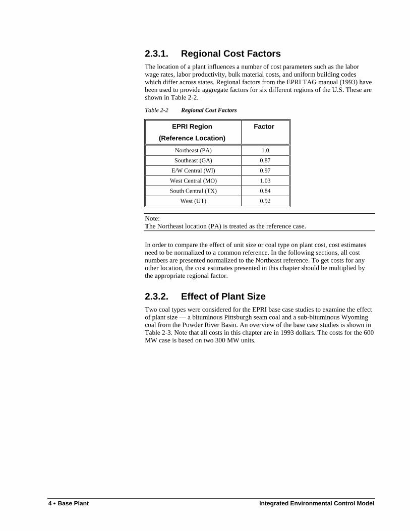
2.3.1. Regional Cost FactorsThe location of a plant influences a number of cost parameters such as the laborwage rates, labor productivity, bulk material costs, and uniform building codeswhich differ across states. Regional factors from the EPRI TAG manual (1993) havebeen used to provide aggregate factors for six different regions of the U.S. These areshown in Table 2-2.
Table 2-2 Regional Cost Factors
EPRI Region
(Reference Location)
Factor
Northeast (PA) 1.0
Southeast (GA) 0.87
E/W Central (WI) 0.97
West Central (MO) 1.03
South Central (TX) 0.84
West (UT) 0.92
Note:The Northeast location (PA) is treated as the reference case.
In order to compare the effect of unit size or coal type on plant cost, cost estimatesneed to be normalized to a common reference. In the following sections, all costnumbers are presented normalized to the Northeast reference. To get costs for anyother location, the cost estimates presented in this chapter should be multiplied bythe appropriate regional factor.
2.3.2. Effect of Plant SizeTwo coal types were considered for the EPRI base case studies to examine the effectof plant size — a bituminous Pittsburgh seam coal and a sub-bituminous Wyomingcoal from the Powder River Basin. An overview of the base case studies is shown inTable 2-3. Note that all costs in this chapter are in 1993 dollars. The costs for the 600MW case is based on two 300 MW units.
Integrated Environmental Control Model Base Plant •••• 5
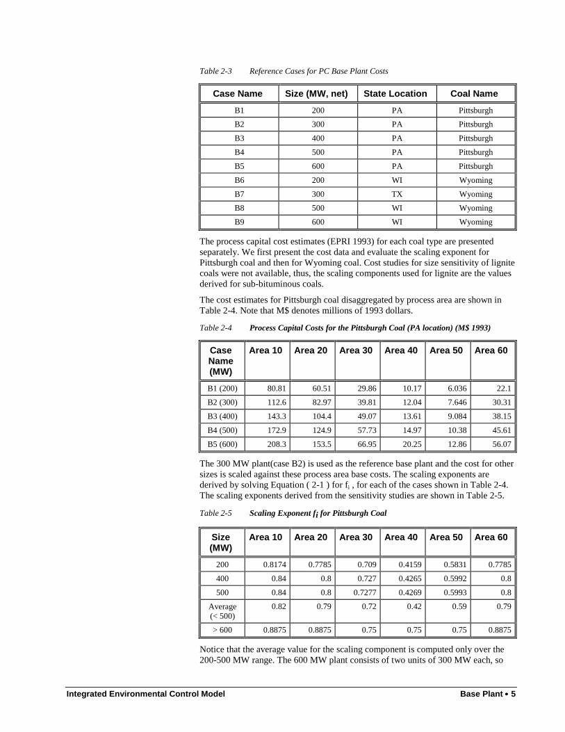
Table 2-3 Reference Cases for PC Base Plant Costs
Case Name Size (MW, net) State Location Coal Name
B1 200 PA Pittsburgh
B2 300 PA Pittsburgh
B3 400 PA Pittsburgh
B4 500 PA Pittsburgh
B5 600 PA Pittsburgh
B6 200 WI Wyoming
B7 300 TX Wyoming
B8 500 WI Wyoming
B9 600 WI Wyoming
The process capital cost estimates (EPRI 1993) for each coal type are presentedseparately. We first present the cost data and evaluate the scaling exponent forPittsburgh coal and then for Wyoming coal. Cost studies for size sensitivity of lignitecoals were not available, thus, the scaling components used for lignite are the valuesderived for sub-bituminous coals.
The cost estimates for Pittsburgh coal disaggregated by process area are shown inTable 2-4. Note that M$ denotes millions of 1993 dollars.
Table 2-4 Process Capital Costs for the Pittsburgh Coal (PA location) (M$ 1993)
CaseName(MW)
Area 10 Area 20 Area 30 Area 40 Area 50 Area 60
B1 (200) 80.81 60.51 29.86 10.17 6.036 22.1
B2 (300) 112.6 82.97 39.81 12.04 7.646 30.31
B3 (400) 143.3 104.4 49.07 13.61 9.084 38.15
B4 (500) 172.9 124.9 57.73 14.97 10.38 45.61
B5 (600) 208.3 153.5 66.95 20.25 12.86 56.07
The 300 MW plant(case B2) is used as the reference base plant and the cost for othersizes is scaled against these process area base costs. The scaling exponents arederived by solving Equation ( 2-1 ) for fi , for each of the cases shown in Table 2-4.The scaling exponents derived from the sensitivity studies are shown in Table 2-5.
Table 2-5 Scaling Exponent fi for Pittsburgh Coal
Size(MW)
Area 10 Area 20 Area 30 Area 40 Area 50 Area 60
200 0.8174 0.7785 0.709 0.4159 0.5831 0.7785
400 0.84 0.8 0.727 0.4265 0.5992 0.8
500 0.84 0.8 0.7277 0.4269 0.5993 0.8
Average(< 500)
0.82 0.79 0.72 0.42 0.59 0.79
> 600 0.8875 0.8875 0.75 0.75 0.75 0.8875
Notice that the average value for the scaling component is computed only over the200-500 MW range. The 600 MW plant consists of two units of 300 MW each, so
6 •••• Base Plant Integrated Environmental Control Model
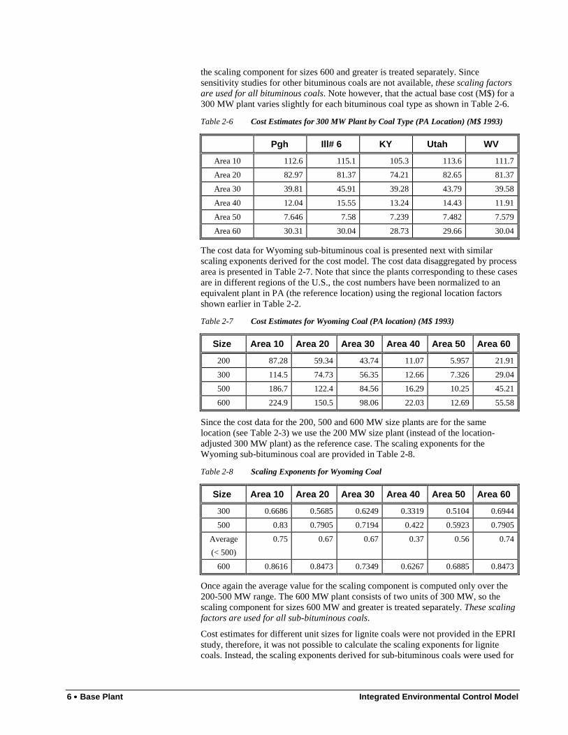
the scaling component for sizes 600 and greater is treated separately. Sincesensitivity studies for other bituminous coals are not available, these scaling factorsare used for all bituminous coals. Note however, that the actual base cost (M$) for a300 MW plant varies slightly for each bituminous coal type as shown in Table 2-6.
Table 2-6 Cost Estimates for 300 MW Plant by Coal Type (PA Location) (M$ 1993)
Pgh Ill# 6 KY Utah WV
Area 10 112.6 115.1 105.3 113.6 111.7
Area 20 82.97 81.37 74.21 82.65 81.37
Area 30 39.81 45.91 39.28 43.79 39.58
Area 40 12.04 15.55 13.24 14.43 11.91
Area 50 7.646 7.58 7.239 7.482 7.579
Area 60 30.31 30.04 28.73 29.66 30.04
The cost data for Wyoming sub-bituminous coal is presented next with similarscaling exponents derived for the cost model. The cost data disaggregated by processarea is presented in Table 2-7. Note that since the plants corresponding to these casesare in different regions of the U.S., the cost numbers have been normalized to anequivalent plant in PA (the reference location) using the regional location factorsshown earlier in Table 2-2.
Table 2-7 Cost Estimates for Wyoming Coal (PA location) (M$ 1993)
Size Area 10 Area 20 Area 30 Area 40 Area 50 Area 60
200 87.28 59.34 43.74 11.07 5.957 21.91
300 114.5 74.73 56.35 12.66 7.326 29.04
500 186.7 122.4 84.56 16.29 10.25 45.21
600 224.9 150.5 98.06 22.03 12.69 55.58
Since the cost data for the 200, 500 and 600 MW size plants are for the samelocation (see Table 2-3) we use the 200 MW size plant (instead of the location-adjusted 300 MW plant) as the reference case. The scaling exponents for theWyoming sub-bituminous coal are provided in Table 2-8.
Table 2-8 Scaling Exponents for Wyoming Coal
Size Area 10 Area 20 Area 30 Area 40 Area 50 Area 60
300 0.6686 0.5685 0.6249 0.3319 0.5104 0.6944
500 0.83 0.7905 0.7194 0.422 0.5923 0.7905
Average
(< 500)
0.75 0.67 0.67 0.37 0.56 0.74
600 0.8616 0.8473 0.7349 0.6267 0.6885 0.8473
Once again the average value for the scaling component is computed only over the200-500 MW range. The 600 MW plant consists of two units of 300 MW, so thescaling component for sizes 600 MW and greater is treated separately. These scalingfactors are used for all sub-bituminous coals.
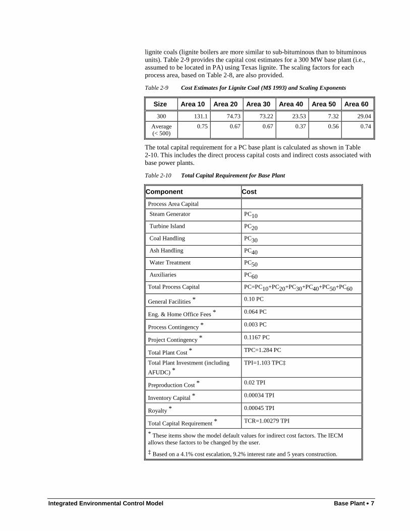
Cost estimates for different unit sizes for lignite coals were not provided in the EPRIstudy, therefore, it was not possible to calculate the scaling exponents for lignitecoals. Instead, the scaling exponents derived for sub-bituminous coals were used for
Integrated Environmental Control Model Base Plant •••• 7
lignite coals (lignite boilers are more similar to sub-bituminous than to bituminousunits). Table 2-9 provides the capital cost estimates for a 300 MW base plant (i.e.,assumed to be located in PA) using Texas lignite. The scaling factors for eachprocess area, based on Table 2-8, are also provided.
Table 2-9 Cost Estimates for Lignite Coal (M$ 1993) and Scaling Exponents
Size Area 10 Area 20 Area 30 Area 40 Area 50 Area 60
300 131.1 74.73 73.22 23.53 7.32 29.04
Average(< 500)
0.75 0.67 0.67 0.37 0.56 0.74
The total capital requirement for a PC base plant is calculated as shown in Table2-10. This includes the direct process capital costs and indirect costs associated withbase power plants.
Table 2-10 Total Capital Requirement for Base Plant
Component Cost
Process Area Capital
Steam Generator PC10
Turbine Island PC20
Coal Handling PC30
Ash Handling PC40
Water Treatment PC50
Auxiliaries PC60
Total Process Capital PC=PC10+PC20+PC30+PC40+PC50+PC60
General Facilities * 0.10 PC
Eng. & Home Office Fees * 0.064 PC
Process Contingency * 0.003 PC
Project Contingency * 0.1167 PC
Total Plant Cost * TPC=1.284 PC
Total Plant Investment (including
AFUDC) *TPI=1.103 TPC‡
Preproduction Cost * 0.02 TPI
Inventory Capital * 0.00034 TPI
Royalty * 0.00045 TPI
Total Capital Requirement * TCR=1.00279 TPI
* These items show the model default values for indirect cost factors. The IECMallows these factors to be changed by the user.
‡ Based on a 4.1% cost escalation, 9.2% interest rate and 5 years construction.
8 •••• Base Plant Integrated Environmental Control Model
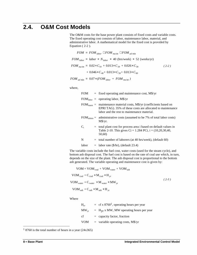
2.4. O&M Cost ModelsThe O&M costs for the base power plant consists of fixed costs and variable costs.The fixed operating cost consists of labor, maintenance labor, material, andadministrative labor. A mathematical model for the fixed cost is provided byEquation ( 2-2 ).
) + FOM(FOM. FOM
C.+ C.+ C.+
C. + C. + C. FOM
N labor FOM
FOMFOM FOMFOM
malaborad
ma
laborlabor
admalabor
intmin
605040
302010int
minint
070
013001300460
02600130020
(weeks/yr)52(hrs/week)40
×=
×××
×××=
×××=
++=
( 2-2 )
where,
FOM = fixed operating and maintenance cost, M$/yr
FOMlabor = operating labor, M$/yr
FOMmaint = maintenance material costs, M$/yr (coefficients based onEPRI TAG). 35% of these costs are allocated to maintenancelabor and the rest to maintenance material.
FOMadmin = administrative costs (assumed to be 7% of total labor costs)M$/yr.
Ci = total plant cost for process area i based on default values inTable 2-10. This gives Ci = 1.284 PCi, i = (10,20,30,40,50,60)
N = total number of laborers (at 40 hrs/week), (default 60)
labor = labor rate ($/hr), (default 23.4)
The variable costs include the fuel cost, water costs (used for the steam cycle), andbottom ash disposal cost. The fuel cost is based on the rate of coal use which, in turn,depends on the size of the plant. The ash disposal cost is proportional to the bottomash generated. The variable operating and maintenance cost is given by:
yrashashash
yrwaterwaterwater
yrcoalcoalcoal
ashwatercoal
HMC = VOM
MW M C = VOM
H M C = VOM
VOM +VOM + VOM = VOM
××
××
××( 2-3 )
Where
Hyr = cf x 87601, operating hours per year
MWyr = Hyr x MW, MW operating hours per year
cf = capacity factor, fraction
VOM = variable operating costs, M$/yr 1 8760 is the total number of hours in a year (24x365)
Integrated Environmental Control Model Base Plant •••• 9
VOMcoal = fuel (coal) costs, M$/yr
VOMwater = water consumption costs, M$/yr
VOMash = ash disposal costs, M$/yr
Mcoal = coal consumption, tons/hr
Mwater = water consumption, gallons/MWh (default = 1000)
Mash = bottom ash disposed, tons/hr
Ccoal = as-delivered coal cost, $/ton
Cash = bottom ash disposal cost, $/ton, (default 10.24)
Cwater = water cost, $/gallon, (default = 0.7 per 1000 gallons)
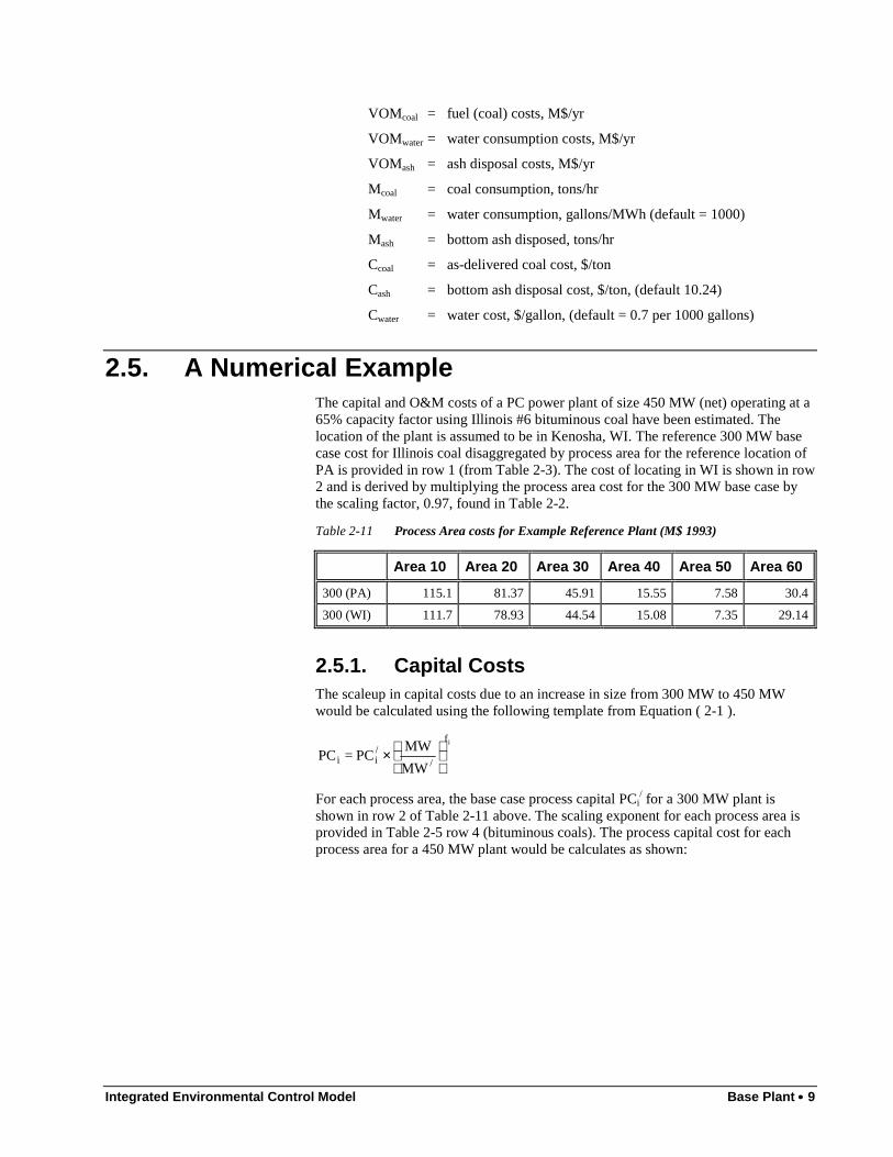
2.5. A Numerical ExampleThe capital and O&M costs of a PC power plant of size 450 MW (net) operating at a65% capacity factor using Illinois #6 bituminous coal have been estimated. Thelocation of the plant is assumed to be in Kenosha, WI. The reference 300 MW basecase cost for Illinois coal disaggregated by process area for the reference location ofPA is provided in row 1 (from Table 2-3). The cost of locating in WI is shown in row2 and is derived by multiplying the process area cost for the 300 MW base case bythe scaling factor, 0.97, found in Table 2-2.
Table 2-11 Process Area costs for Example Reference Plant (M$ 1993)
Area 10 Area 20 Area 30 Area 40 Area 50 Area 60
300 (PA) 115.1 81.37 45.91 15.55 7.58 30.4
300 (WI) 111.7 78.93 44.54 15.08 7.35 29.14
2.5.1. Capital CostsThe scaleup in capital costs due to an increase in size from 300 MW to 450 MWwould be calculated using the following template from Equation ( 2-1 ).
if
//ii
MW
MWPC = PC
×
For each process area, the base case process capital PCi/ for a 300 MW plant is
shown in row 2 of Table 2-11 above. The scaling exponent for each process area isprovided in Table 2-5 row 4 (bituminous coals). The process capital cost for eachprocess area for a 450 MW plant would be calculates as shown:

10 •••• Base Plant Integrated Environmental Control Model
M 40.14 = 300
450 M 29.14 = PC
M 9.34 = 300
450 M 7.35 = PC
M 17.88 = 300
450 M 15.08 = PC
M 59.64 = 300
450 M 44.54 = PC
M 108.73 = 300
450 M 78.93 = PC
M 155.76 = 300
450 M 111.7 = PC
79.0
60
59.0
50
42.0
40
72.0
30
79.0
20
82.0
10
×
×
×
×
×
×
( )
$/kW 1256 = M$ 565.85 =t Requiremen Capital Total
M$ 0.25 = TPI 0.00045 =Royalty
M$ 0.19 = TPI 0.00034 = CapitalInventory
M$ 11.09 = TPI 0.02 = Costsion Preproduct
M$ 554.32 = 502.56 1.03 = (TPI) InvestmentPlant Total
M$ 502.56 = C+C+EHO+GFC+PC = (TPC)Cost Plant Total
M$ 45.69= 391.49 0.1167 = )(Cy ContingencProject
M$ 1.17= 391.49 0.003 = )(Cy Contingenc Process
M$ 25.06= 391.49 0.064 = (EHO) Office Home&Eng.
M$ 39.15 = 391.49 0.10 = (GFC) Facilities General
M$ 391.49 = PC = (PC) Capital Process Total
projproc
proj
proc
i
×
×
×
×
×
×
×
×
∑
∑
2.5.2. Fixed O&M Costs:The fixed O&M costs are calculated using Equation ( 2-2 ). The formulae fromEquation ( 2-2 ) reproduced here with appropriate numeric values. Text is providedin brackets next to each number to explain the source of these numbers. Note that thetotal plant cost for each process area (denoted by Ci) is calculated as Ci = 1.284 PCi.
Integrated Environmental Control Model Base Plant •••• 11
M$/yr 13.49 =
)(FOM 0.88 )(FOM 9.69 )(FOM 2.92 = FOM
M$/yr 0.88 = ))(FOM 9.689 +)(FOM (2.920.07 =FOM
M$/yr 9.69 =
)(C 51.50.013 +)(C 11.990.013+
)(C 22.960.046 +)(C 76.6 0.026+
)(C 139.6 0.013 + )(C 199.9 0.02 =FOM
M$/yr 2.92 =
(weeks/yr) 52 (hrs/week) 40
laborers) (60 N $/hr) (23.4labor =FOM
adminmaintlabor
maintlaboradmin
6050
4030
2010maint
laborlabor
++
×
××
××
××
××
×
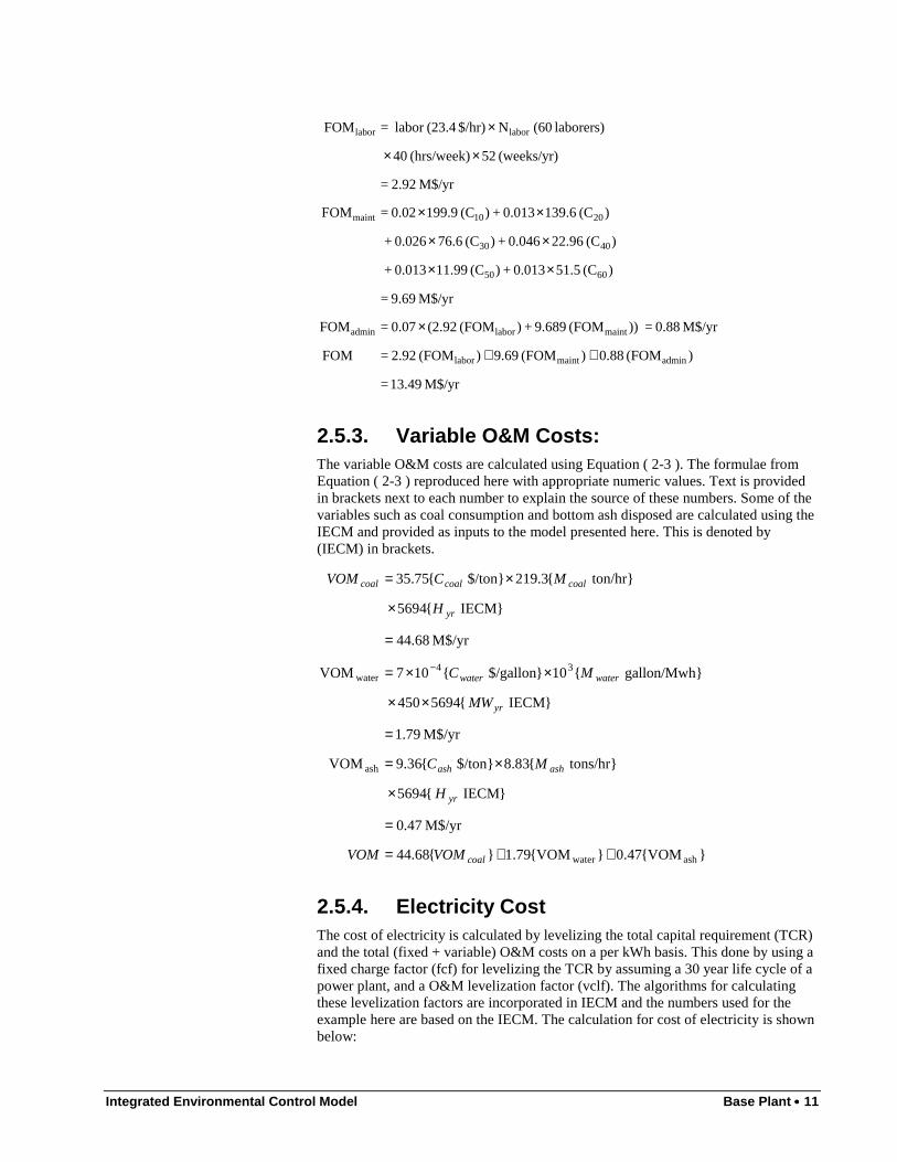
2.5.3. Variable O&M Costs:The variable O&M costs are calculated using Equation ( 2-3 ). The formulae fromEquation ( 2-3 ) reproduced here with appropriate numeric values. Text is providedin brackets next to each number to explain the source of these numbers. Some of thevariables such as coal consumption and bottom ash disposed are calculated using theIECM and provided as inputs to the model presented here. This is denoted by(IECM) in brackets.
}VOM{47.0}VOM{79.1}{68.44
M$/yr 47.0
}IECM {5694
} tons/hr{83.8}$/ton {36.9VOM
M$/yr 79.1
}IECM {5694450
}gallon/Mwh {10}$/gallon {107VOM
M$/yr 68.44
}IECM {5694
} ton/hr{3.219}$/ton {75.35
ashwater
ash
34water
++=
=
×
×=
=
××
××=
=
×
×=
−
coal
yr
ashash
yr
waterwater
yr
coalcoalcoal
VOMVOM
H
MC
MW
MC
H
MCVOM
2.5.4. Electricity CostThe cost of electricity is calculated by levelizing the total capital requirement (TCR)and the total (fixed + variable) O&M costs on a per kWh basis. This done by using afixed charge factor (fcf) for levelizing the TCR by assuming a 30 year life cycle of apower plant, and a O&M levelization factor (vclf). The algorithms for calculatingthese levelization factors are incorporated in IECM and the numbers used for theexample here are based on the IECM. The calculation for cost of electricity is shownbelow:
12 •••• Base Plant Integrated Environmental Control Model
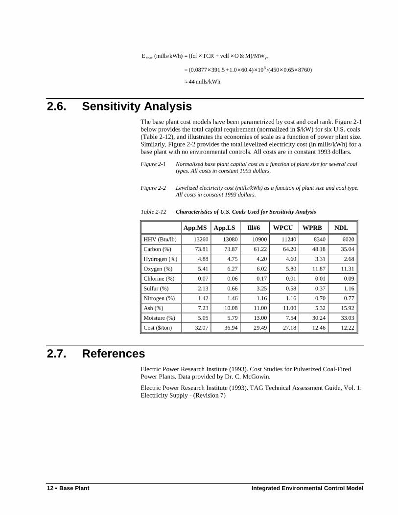
mills/kWh 44
8760)0.65/(4501060.4)1.0 + 391.5(0.0877 =
M)/MW&O vclf+ TCR(fcf =)(mills/kWh E
6
yrcost
≈
×××××
××
2.6. Sensitivity AnalysisThe base plant cost models have been parametrized by cost and coal rank. Figure 2-1below provides the total capital requirement (normalized in $/kW) for six U.S. coals(Table 2-12), and illustrates the economies of scale as a function of power plant size.Similarly, Figure 2-2 provides the total levelized electricity cost (in mills/kWh) for abase plant with no environmental controls. All costs are in constant 1993 dollars.
Figure 2-1 Normalized base plant capital cost as a function of plant size for several coaltypes. All costs in constant 1993 dollars.
Figure 2-2 Levelized electricity cost (mills/kWh) as a function of plant size and coal type.All costs in constant 1993 dollars.
Table 2-12 Characteristics of U.S. Coals Used for Sensitivity Analysis
App.MS App.LS Ill#6 WPCU WPRB NDL
HHV (Btu/lb) 13260 13080 10900 11240 8340 6020
Carbon (%) 73.81 73.87 61.22 64.20 48.18 35.04
Hydrogen (%) 4.88 4.75 4.20 4.60 3.31 2.68
Oxygen (%) 5.41 6.27 6.02 5.80 11.87 11.31
Chlorine (%) 0.07 0.06 0.17 0.01 0.01 0.09
Sulfur (%) 2.13 0.66 3.25 0.58 0.37 1.16
Nitrogen (%) 1.42 1.46 1.16 1.16 0.70 0.77
Ash (%) 7.23 10.08 11.00 11.00 5.32 15.92
Moisture (%) 5.05 5.79 13.00 7.54 30.24 33.03
Cost ($/ton) 32.07 36.94 29.49 27.18 12.46 12.22
2.7. ReferencesElectric Power Research Institute (1993). Cost Studies for Pulverized Coal-FiredPower Plants. Data provided by Dr. C. McGowin.
Electric Power Research Institute (1993). TAG Technical Assessment Guide, Vol. 1:Electricity Supply - (Revision 7)
Integrated Environmental Control Model Selective Catalytic Reduction •••• 13
3. Selective Catalytic Reduction
3.1. Introduction to SCR TechnologySelective catalytic reduction (SCR) is a process for the post-combustion removal ofNOx from the flue gas of fossil-fuel-fired power plants. SCR is capable of NOx
reduction efficiencies of up to 80 or 90 percent. SCR technology has been applied fortreatment of flue gases from a variety of emission sources, including natural gas- andoil-fired gas turbines, process steam boilers in refineries, and coal-fired power plants.SCR applications to coal-fired power plants have occurred in Japan and Germany.Full-scale SCR systems have not been applied to coal-fired power plants in the U.S.,although there have been small-scale demonstration projects.
Increasingly strict NOx control requirements are being imposed by various state andlocal regulatory agencies in the U. S. These requirements may lead to U.S. SCRapplications, particularly for plants burning low sulfur coals (Robie et al., 1991).Furthermore, implicit in Title IV of the 1990 Clean Air Act Amendment is a nationalNOx emission reduction of 2 million tons per year. Thus, there may be otherincentives to adapt SCR technology more generally to U.S. coal-fired power plantswith varying coal sulfur contents. However, concern remains over the applicabilityof SCR technology to U.S. plants burning high sulfur coals or coals withsignificantly different fly ash characteristics than those burned in Germany andJapan. There is also concern regarding the application of SCR to peaking units due topotential startup and shutdown problems (Lowe et al., 1991).
3.2. Process History and DevelopmentSCR was invented and patented in the U.S. in 1959. It was used originally inindustrial applications. In the 1970's, SCR was first applied in Japan for control ofNOx emissions from power plants. Japan was the first country to make widespreaduse of this technology in response to national emission standards for NOx. In Japan,SCR has been applied to gas, oil, and coal-fired power plants. There were over 200commercial SCR systems operating on all types of sources in Japan in 1985. TheJapanese SCR systems tend to run at moderate NOx removal efficiencies of 40 to 60percent (Gouker and Brundrett, 1991). By 1990, a total of 40 systems had beeninstalled on 10,852 MW of coal-fired power plants (Lowe et al., 1991).
Germany currently imposes more stringent NOx emission standards than Japan. Tomeet the emission requirements, SCR has been adopted and applied to many coal-fired power plants. SCR will be required as a retrofit technology on a total of 37,500MW of existing capacity. As of 1989, SCR had been applied in 70 pilot plants and

14 •••• Selective Catalytic Reduction Integrated Environmental Control Model
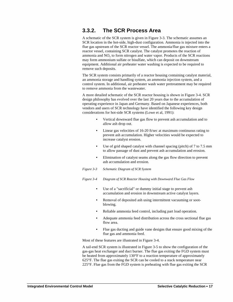
28 full scale retrofit installations, with the latter totaling 7,470 MW of hard coal-firedcapacity (Schönbucher, 1989). By 1990, more than 23,000 MW of capacity werefitted with SCR systems (Gouker and Brundrett, 1991). These plants typically burnlow sulfur coals (0.8 to 1.5 percent sulfur) with 0.1 to 0.3 percent chlorine. SCR hasbeen retrofitted to power plants with both wet and dry bottom boilers, with variationson the location of the SCR system. As of 1989, 18 installations involve placement ofthe SCR system between the economizer and air preheater, while the remaininginvolve "low dust" or "tail-end" placement of the SCR downstream of the FGDsystem. Two of the high-dust retrofits involve wet bottom boilers (Schönbucher,1989). In 1991, 129 systems were reported to have been installed on a total of 30,625MW of coal-fired capacity (Lowe et al., 1991). The recent German progress ininstalling retrofit SCR systems is shown graphically in Figure 3-1.
The process environment for SCR in Germany is typically more demanding than thatin Japan, with the requirement for higher NOx removal with higher flue gas sulfurand ash loadings (Gouker and Brundrett, 1991). In both Japan and Germany, theSCR systems are not operated during startup or shutdown (Lowe et al., 1991).
SCR is being applied in the U.S. for NOx control of natural gas and oil-fired gasturbine-based power generation systems. In 1990 SCR was installed at a total of 110gas turbine units totaling 3,600 MW (May et al, 1991). While the operatingenvironment for these systems is not as demanding as for coal-fired power plantapplications, some of these applications do provide experience with systems firingsulfur-bearing fuels that encounter problems analogous to those anticipated in coal-based applications. In particular, ammonium salt formation and downstream effectshave been studied (Johnson et al, 1990).
Recently, a number of U.S. projects for coal-fired applications of SCR technologyhave been initiated. These include, for example, a U.S. Department of Energy CleanCoal Program funded demonstration of SCR at Gulf Power Company's Plant Crist(DOE, 1992). SCR systems have also been permitted for two coal-fired cogenerationplants to be built in New Jersey (Fickett, 1993).
Since the 1970's, the cost of SCR has dropped substantially. For example, thelevelized cost of SCR dropped by a factor of 3 in Japan within a 6 year period, whilein recent years costs in Germany have dropped by an additional factor of 2. Theseimprovements are due in part to the international competition among catalystsuppliers. SCR catalysts are available from manufacturers in Japan, Germany, andthe U.S. U.S. manufacturers, such as Grace, expect improvements in catalysts tocontinue, resulting in potential further drops in capital and operating costs. Forexample, Grace is testing a new catalyst design that is expected to lead to a 50percent increase in catalyst activity while also increasing catalyst life (Gouker andBrundrett, 1991).
1989 1990 19910
10000
20000
30000
40000
���������������������������������������������������������������������������
������������������������������������������������������������������������������������������������������������������������������������������������������
��������������������������������������������������������������������������������������������������������������������������������������������������������������������������������������������������������
����Installed
37,500 MW
Year
Cap
acity
, M
W
Target
Capacity
Figure 3-1 Targeted and Actual Installed Retrofit SCR Capacity in Germany
Integrated Environmental Control Model Selective Catalytic Reduction •••• 15
SCR has not yet been used commercially on coal-fired power plants in the U.S. Theexperience in Germany, which includes boiler types similar to those in the U.S.,provides useful data for predicting SCR performance and cost in the U.S. However,U.S. coals, such as eastern bituminous coals, typically have a higher sulfur contentthan that of German coals. In addition, fly ash compositions may vary significantly.These differences lead to concerns about maintenance of catalyst activity andpotential difficulties downstream of SCR reactors, such as deposition of ammoniasalts.
The German experience is particularly useful for U.S. planners because German SCRsystems are subject to a more relevant range of flue gas conditions than typicalJapanese systems. For example, slagging wet bottom boilers produce different fluegas and flyash characteristics that can significantly affect catalyst performance(Offen et al, 1987).
3.3. Process DesignThe general design considerations for the SCR NOx control technology for coal-firedpower plants are described here. These include the placement of the SCR system in apower plant, and a description of equipment associated with the SCR process area.
3.3.1. SCR Integration in the Power PlantThe SCR system can be located in several places in the coal-fired power plant fluegas stream (Schönbucher, 1989; Behrens et al, 1991). A key limitation of SCRsystems is the operating temperature requirement. The operating temperaturewindow for SCR systems is typically from approximately 550 to 750°F. Severalpossible locations are illustrated inFigure 3-2. These are:
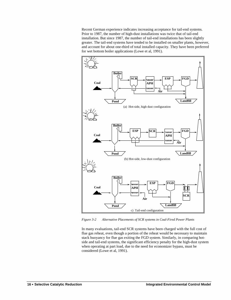
1. "Hot-side" and "high-dust" SCR, with the reactor located between theeconomizer and the air preheater. In this configuration, shown in Figure3-2a, the SCR is located upstream of a cold-side ESP and, hence, issubject to a high fly ash or "dust" loading. At full-load, the economizeroutlet temperature is typically around 700°F. An economizer bypass isrequired to supply hot gas to the SCR during part-load operatingconditions, in order to maintain the proper reaction temperatures (Loweet al, 1991).
2. "Hot-side, low-dust" SCR, which features placement of the SCRsystem downstream of a hot-side ESP and upstream of the air preheaterand FGD systems. This configuration has been employed in someJapanese coal-fired power plants, such as Takehara Power Station Unit1 in Hiroshima (Behrens et al, 1991). This configuration has theadvantage of minimizing the fly ash loading to the SCR catalyst, whichleads to degradation in catalyst performance.
3. "Cold-side" or "Tail-end" placement of the SCR system downstream ofthe air preheater, particulate collector, and FGD system. This systemminimizes the effects that flue gas contaminants have on SCR catalystdesign and operation, but requires a gas-gas flue gas heat exchangerand duct burners to bring the flue gas up to reaction temperature (Loweet al, 1991).
The most common configurations envisioned for U.S. power plants are the hot-sidehigh-dust and post-FGD tail-end systems (Robie et al, 1991), with high-dust systemspredominating. These are the two most common configurations employed in Germancoal-fired power plants retrofitted with SCR.
16 •••• Selective Catalytic Reduction Integrated Environmental Control Model
Recent German experience indicates increasing acceptance for tail-end systems.Prior to 1987, the number of high-dust installations was twice that of tail-endinstallation. But since 1987, the number of tail-end installations has been slightlygreater. The tail-end systems have tended to be installed on smaller plants, however,and account for about one-third of total installed capacity. They have been preferredfor wet bottom boiler applications (Lowe et al, 1991).
ESP FGD
��������������������������������������������
SCR
APH
Air
LandfillPond
Boiler
Coal
ESP FGD
LandfillPond
Boiler
Coal APH
Air
���������������������������������SCR
(a) Hot-side, high dust configuration
(b) Hot-side, low-dust configuration
c) Tail-end configuration
Pond
Boiler
FGD
APH
Air
CoalESP
Landfill
���������������������������������SCR
Figure 3-2 Alternative Placements of SCR systems in Coal-Fired Power Plants
In many evaluations, tail-end SCR systems have been charged with the full cost offlue gas reheat, even though a portion of the reheat would be necessary to maintainstack buoyancy for flue gas exiting the FGD system. Similarly, in comparing hot-side and tail-end systems, the significant efficiency penalty for the high-dust systemwhen operating at part load, due to the need for economizer bypass, must beconsidered (Lowe et al, 1991).
Integrated Environmental Control Model Selective Catalytic Reduction •••• 17
3.3.2. The SCR Process AreaA schematic of the SCR system is given in Figure 3-3. The schematic assumes anSCR location in the hot-side, high-dust configuration. Ammonia is injected into theflue gas upstream of the SCR reactor vessel. The ammonia/flue gas mixture enters areactor vessel, containing SCR catalyst. The catalyst promotes the reaction ofammonia and NOx to form nitrogen and water vapor. Products of the SCR reactionsmay form ammonium sulfate or bisulfate, which can deposit on downstreamequipment. Additional air preheater water washing is expected to be required toremove such deposits.
The SCR system consists primarily of a reactor housing containing catalyst material,an ammonia storage and handling system, an ammonia injection system, and acontrol system. In additional, air preheater wash water pretreatment may be requiredto remove ammonia from the wastewater.
A more detailed schematic of the SCR reactor housing is shown in Figure 3-4. SCRdesign philosophy has evolved over the last 20 years due to the accumulation ofoperating experience in Japan and Germany. Based on Japanese experiences, bothvendors and users of SCR technology have identified the following key designconsiderations for hot-side SCR systems (Lowe et al, 1991):
• Vertical downward flue gas flow to prevent ash accumulation and toallow ash drop out.
• Linear gas velocities of 16-20 ft/sec at maximum continuous rating toprevent ash accumulation. Higher velocities would be expected toincrease catalyst erosion.
• Use of grid shaped catalyst with channel spacing (pitch) of 7 to 7.5 mmto allow passage of dust and prevent ash accumulation and erosion.
• Elimination of catalyst seams along the gas flow direction to preventash accumulation and erosion.
Figure 3-3 Schematic Diagram of SCR System
Figure 3-4 Diagram of SCR Reactor Housing with Downward Flue Gas Flow
• Use of a "sacrificial" or dummy initial stage to prevent ashaccumulation and erosion in downstream active catalyst layers.
• Removal of deposited ash using intermittent vacuuming or soot-blowing.
• Reliable ammonia feed control, including part load operation.
• Adequate ammonia feed distribution across the cross sectional flue gasflow area.
• Flue gas ducting and guide vane designs that ensure good mixing of theflue gas and ammonia feed.
Most of these features are illustrated in Figure 3-4.
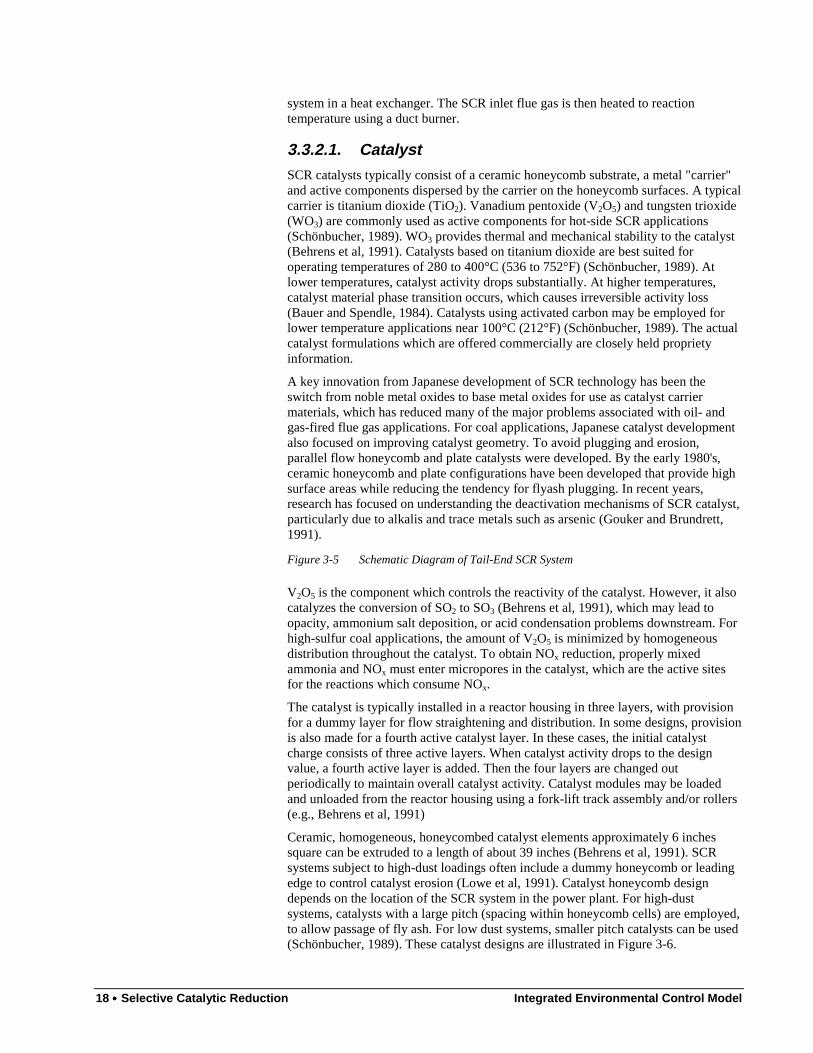
A tail-end SCR system is illustrated in Figure 3-5 to show the configuration of thegas-gas heat exchanger and duct burner. The flue gas exiting the FGD system mustbe heated from approximately 130°F to a reaction temperature of approximately625°F. The flue gas exiting the SCR can be cooled to a stack temperature near225°F. Flue gas from the FGD system is preheating with flue gas exiting the SCR
18 •••• Selective Catalytic Reduction Integrated Environmental Control Model
system in a heat exchanger. The SCR inlet flue gas is then heated to reactiontemperature using a duct burner.
3.3.2.1. CatalystSCR catalysts typically consist of a ceramic honeycomb substrate, a metal "carrier"and active components dispersed by the carrier on the honeycomb surfaces. A typicalcarrier is titanium dioxide (TiO2). Vanadium pentoxide (V2O5) and tungsten trioxide(WO3) are commonly used as active components for hot-side SCR applications(Schönbucher, 1989). WO3 provides thermal and mechanical stability to the catalyst(Behrens et al, 1991). Catalysts based on titanium dioxide are best suited foroperating temperatures of 280 to 400°C (536 to 752°F) (Schönbucher, 1989). Atlower temperatures, catalyst activity drops substantially. At higher temperatures,catalyst material phase transition occurs, which causes irreversible activity loss(Bauer and Spendle, 1984). Catalysts using activated carbon may be employed forlower temperature applications near 100°C (212°F) (Schönbucher, 1989). The actualcatalyst formulations which are offered commercially are closely held proprietyinformation.
A key innovation from Japanese development of SCR technology has been theswitch from noble metal oxides to base metal oxides for use as catalyst carriermaterials, which has reduced many of the major problems associated with oil- andgas-fired flue gas applications. For coal applications, Japanese catalyst developmentalso focused on improving catalyst geometry. To avoid plugging and erosion,parallel flow honeycomb and plate catalysts were developed. By the early 1980's,ceramic honeycomb and plate configurations have been developed that provide highsurface areas while reducing the tendency for flyash plugging. In recent years,research has focused on understanding the deactivation mechanisms of SCR catalyst,particularly due to alkalis and trace metals such as arsenic (Gouker and Brundrett,1991).
Figure 3-5 Schematic Diagram of Tail-End SCR System
V2O5 is the component which controls the reactivity of the catalyst. However, it alsocatalyzes the conversion of SO2 to SO3 (Behrens et al, 1991), which may lead toopacity, ammonium salt deposition, or acid condensation problems downstream. Forhigh-sulfur coal applications, the amount of V2O5 is minimized by homogeneousdistribution throughout the catalyst. To obtain NOx reduction, properly mixedammonia and NOx must enter micropores in the catalyst, which are the active sitesfor the reactions which consume NOx.
The catalyst is typically installed in a reactor housing in three layers, with provisionfor a dummy layer for flow straightening and distribution. In some designs, provisionis also made for a fourth active catalyst layer. In these cases, the initial catalystcharge consists of three active layers. When catalyst activity drops to the designvalue, a fourth active layer is added. Then the four layers are changed outperiodically to maintain overall catalyst activity. Catalyst modules may be loadedand unloaded from the reactor housing using a fork-lift track assembly and/or rollers(e.g., Behrens et al, 1991)
Ceramic, homogeneous, honeycombed catalyst elements approximately 6 inchessquare can be extruded to a length of about 39 inches (Behrens et al, 1991). SCRsystems subject to high-dust loadings often include a dummy honeycomb or leadingedge to control catalyst erosion (Lowe et al, 1991). Catalyst honeycomb designdepends on the location of the SCR system in the power plant. For high-dustsystems, catalysts with a large pitch (spacing within honeycomb cells) are employed,to allow passage of fly ash. For low dust systems, smaller pitch catalysts can be used(Schönbucher, 1989). These catalyst designs are illustrated in Figure 3-6.

Integrated Environmental Control Model Selective Catalytic Reduction •••• 19
3.3.2.2. Ammonia HandlingIn Germany, strict safety standards have been applied to the shipment and handlingof ammonia. Shipments by truck are not permitted if they are larger than 500 liters.Thus, anhydrous ammonia is shipped primarily by rail. A 15 to 30 day supply istypically stored at the plant in two double wall tanks. Double walled piping is alsotypically employed. The ammonia is diluted to an 8 percent mixture prior tointroduction to the flue gas. The ammonia is vaporized in German facilities usingwarm water. In many U.S. gas turbine installations, electrical heating is used (Loweet al, 1991).
3.4. Technical OverviewThis section presents a detailed technical overview of SCR NOx control technologyfor coal-fired power plants, with particular focus on the effects of flue gascomponents on catalyst performance and the effects of the SCR system on the powerplant.
������������������������������������������������������������������������������������������������������������������������������������������������������������������������������������������������
������������������������������������������������������������������������������������������������������������������������������������������������������������������������������������������������
������������������������������������������������������������������������������������������������������������������������������������������������������������������������������������������������
��������������������������������������������������������������������������������������������������������������������������������������������������������������������������������
7.5 mm, typ.
4 mm, typ.
(a) Monolith for High-Dust Application (b) Monolith for Tail-End Application
������������������������������������������������������������
������������������������������������������������������������
������������������������������������������������������������
������������������������������������������������������������
����������������������������������������������������������������������
����������������������������������������������������������������������
���������������������������������������������������������������������������������������������������
������������������������������������������������������������������������������������������������������������������������������������
������������������������������������������������������������������������������������������������������������������������������������
���������������������������������������������������������������������������������������������������
���������������������������������������������������������������������������������������������������
���������������������������������������������������������������������������������������������������
������������������������������������������������������������
������������������������������������������������������������
������������������������������������������������������������
������������������������������������������������������������
����������������������������������������������������������������������
����������������������������������������������������������������������
���������������������������������������������������������������������������������������������������
���������������������������������������������������������������������������������������������������
���������������������������������������������������������������������������������������������������
������������������������������������������������������������������������������������������������������������������������������������
������������������������������������������������������������������������������������������������������������������������������������
���������������������������������������������������������������������������������������������������
������������������������������������������������������������
������������������������������������������������������������
������������������������������������������������������������
����������������������������������������������������������������������
������������������������������������������������������������
������������������������������������������������������������
������������������������������������������������������������������������������������������������
��������������������������������������������������������������������������������������������������������������������������������
��������������������������������������������������������������������������������������������������������������������������������
������������������������������������������������������������������������������������������������
������������������������������������������������������������������������������������������������
������������������������������������������������������������������������������������������������
������������������������������������������������������������
������������������������������������������������������������
������������������������������������������������������������
����������������������������������������������������������������������
������������������������������������������������������������
��������������������������������������������������������������������������������������������������������������
������������������������������������������������������������������������������������������������
������������������������������������������������������������������������������������������������
������������������������������������������������������������������������������������������������
��������������������������������������������������������������������������������������������������������������������������������
��������������������������������������������������������������������������������������������������������������������������������
������������������������������������������������������������������������������������������������
������������������������������������������������������������������������������������������������������������������������������������������������������������������������������������������������������������������������������������������������������������������������������������������������������������������������������������������������������������������������������������������������������������������������������������������������������������������������������������������������������������������������������������������������������������������������������������������������������������������������������������������������������������������������������������������������������������������������������������������������������������������������������������������������������������������������������������������������������������������������������������������������������������������������������������������������������������������������������������������������������������������������������������������������������������������������������������������������������������������������������������������������������������������������������������������������������������������������������������������������
�������������������������������������������������������������������������������������������������������������������������������������������������������������������������������������������������������������������������������������������������������������������������������������������������������������������������������������
�������������������������������������������������������������������������������������������������������������������������������������������������������������������������������������������������������������������������������������������������������������������������������������������������������������������������������������
��������������������������������������������������������������������������������������������������������������������������������������������������������������������������������������������������������������������������������������������������������������������
��������������������������������������������������������������������������������������������������������������������������������������������������������������������������������������������������������������������������������������������������������������������
�������������������������������������������������������������������������������������������������������������������������������������������������������������������������������������������������������������������������������������������������������������������������������������������������������������������������������������
�������������������������������������������������������������������������������������������������������������������������������������������������������������������������������������������������������������������������������������������������������������������������������������������������������������������������������������
����������������������������������������������������������������������������������������������������������������������������������������������������������������������������������������������������������������������������������������������������������������������������������������������������������������������������������������������������������������������������������������������������������������������������������������������������������������������������������������������������������������������������������������������������������������������������������������������������������������������������������������������������������������������������������������������������������������������������������������������������������������������������������������������������������������������������������������������������������������������������������������������������������������������������������������������������������������������������������������������������������������������������������������������������������������������������������������������������������������������������������������������������������������������������������������������������������������������������������������������������������������
6.1 mm, typ.
Figure 3-6 SCR Honeycomb Catalyst Monolith Designs
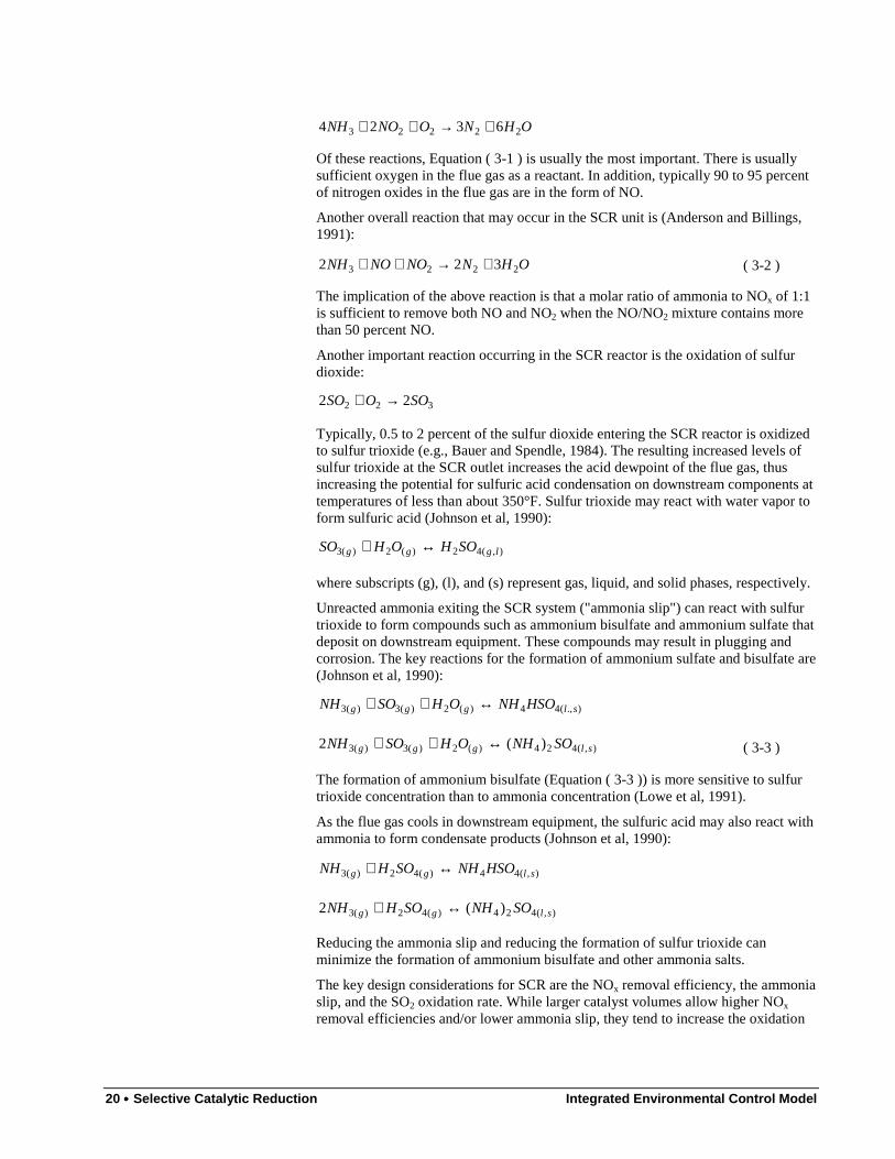
3.4.1. Process ChemistryNitrogen oxides in the flue gas are removed by reduction of NOx by ammonia tonitrogen and water. The reduction occurs in the presence of a catalyst. Ammonia isinjected in the flue gas upstream of the catalyst, as illustrated in Figure 3-3.
The principle reactions are:
OHNNONH 223 6564 +→+
OHNNONH 2223 12768 +→+
OHNONONH 2223 6444 +→++ ( 3-1 )
20 •••• Selective Catalytic Reduction Integrated Environmental Control Model
OHNONONH 22223 6324 +→++
Of these reactions, Equation ( 3-1 ) is usually the most important. There is usuallysufficient oxygen in the flue gas as a reactant. In addition, typically 90 to 95 percentof nitrogen oxides in the flue gas are in the form of NO.
Another overall reaction that may occur in the SCR unit is (Anderson and Billings,1991):
OHNNONONH 2223 322 +→++ ( 3-2 )
The implication of the above reaction is that a molar ratio of ammonia to NOx of 1:1is sufficient to remove both NO and NO2 when the NO/NO2 mixture contains morethan 50 percent NO.
Another important reaction occurring in the SCR reactor is the oxidation of sulfurdioxide:
322 22 SOOSO →+
Typically, 0.5 to 2 percent of the sulfur dioxide entering the SCR reactor is oxidizedto sulfur trioxide (e.g., Bauer and Spendle, 1984). The resulting increased levels ofsulfur trioxide at the SCR outlet increases the acid dewpoint of the flue gas, thusincreasing the potential for sulfuric acid condensation on downstream components attemperatures of less than about 350°F. Sulfur trioxide may react with water vapor toform sulfuric acid (Johnson et al, 1990):
),(42)(2)(3 lggg SOHOHSO ↔+
where subscripts (g), (l), and (s) represent gas, liquid, and solid phases, respectively.
Unreacted ammonia exiting the SCR system ("ammonia slip") can react with sulfurtrioxide to form compounds such as ammonium bisulfate and ammonium sulfate thatdeposit on downstream equipment. These compounds may result in plugging andcorrosion. The key reactions for the formation of ammonium sulfate and bisulfate are(Johnson et al, 1990):
).,(44)(2)(3)(3 slggg HSONHOHSONH ↔++
),(424)(2)(3)(3 )(2 slggg SONHOHSONH ↔++ ( 3-3 )
The formation of ammonium bisulfate (Equation ( 3-3 )) is more sensitive to sulfurtrioxide concentration than to ammonia concentration (Lowe et al, 1991).
As the flue gas cools in downstream equipment, the sulfuric acid may also react withammonia to form condensate products (Johnson et al, 1990):
),(44)(42)(3 slgg HSONHSOHNH ↔+
),(424)(42)(3 )(2 slgg SONHSOHNH ↔+
Reducing the ammonia slip and reducing the formation of sulfur trioxide canminimize the formation of ammonium bisulfate and other ammonia salts.
The key design considerations for SCR are the NOx removal efficiency, the ammoniaslip, and the SO2 oxidation rate. While larger catalyst volumes allow higher NOx
removal efficiencies and/or lower ammonia slip, they tend to increase the oxidation

Integrated Environmental Control Model Selective Catalytic Reduction •••• 21
of SO2. Furthermore, large catalyst volumes significantly increase the capital andannual costs of SCR.
3.4.2. Catalyst SizingA key performance issue associated with SCR systems is the required catalystvolume and the catalyst replacement schedule. One parameter often used to measurecatalyst volume is the space velocity, which is given by:
cFG VGSV /=
An alternative parameter is the area velocity, which is given by:
cFG VGAV /=
The relationship between the space velocity and area velocity depends on the"geometric ratio" of the catalyst, which is the unit surface area per unit volume of thecatalyst.
c
cg
V
AR =
For honeycomb monolith catalysts, the important design parameter that determinesthe geometric ratio is the "pitch," or spacing between the hollow cells through whichthe flue gas passes. As described earlier, the catalyst pitch depends primarily on thedust loading in the flue gas. Larger pitches are needed to accommodate high-dustloadings, resulting in a lower geometric ratio. Current catalysts for high-dustapplication typically have a pitch of around 7.5 mm, with a wall thickness of 1.4 mmand a channel thickness of 6.1 mm. For tail-end applications, pitches of around 4 mmare typical. For gas-fired applications, pitches of 3 mm are reported using ceramicplate-type catalysts. Catalyst using thin metal substrates may have a pitch as low as0.2 mm for clean flue gas applications (Gouker and Brundrett, 1991).
The space velocity is commonly used to describe the catalyst requirement. However,both the space velocity and area ratio, or the space and area velocities, are needed inorder to specify both the catalyst volume and the catalyst area in contact with the fluegas. For example, a high-dust SCR system typically requires a smaller space velocity(more catalyst) than a low-dust system, due primarily to the lower area ratio of thehigh-dust catalyst designs.
The space velocity is a function of the desired NOx removal efficiency and therequired ammonia slip. For example, one EPRI paper suggests a maximum spacevelocity of 2,500/hr for a NOx reduction efficiency of 80 percent and an ammoniaslip of 5 ppm (Damon et al, 1987).
Based on German experience, typical space velocities for high-dust SCR systemswith honeycomb catalysts of about 7 mm pitch are 2,000 to 3,000/hr, whereas fortail-end systems employing honeycomb catalysts with pitches of approximately 4mm space velocities are 4,000 to 6,500/hr. Thus, 50 to 60 percent smaller catalystvolumes per unit flue gas flow can be installed on tail-end systems for equivalentNOx removal performance. However, the flue gas volumetric flow rate may behigher for tail-end systems than for high-dust systems, partially offsetting thisadvantage (Lowe et al, 1991).
The actual required catalyst volume for a given application depends on a number ofsite-specific factors. The amount of plugging or catalyst poisoning will determine theeffective catalyst activity. The activity will decrease with operating time. Therefore,
22 •••• Selective Catalytic Reduction Integrated Environmental Control Model
the initial catalyst volume must be large enough so that at the end of the design lifethere is sufficient active catalyst to maintain design performance levels.
Most SCR designs have a three layer catalyst. Although most U.S. SCR studiesassume that all catalyst layers are changed out simultaneously, most Japanese andGerman designs are based on periodic replacement of only one catalyst layer at atime. Therefore, at any given time, there may be three layers with differing lengths ofservice and differing activity levels. In determining the initial catalyst charge, it isnecessary to account for the loss of catalyst activity at the design point in the catalystreplacement scheme. For a three layer catalyst, the design point is the fourth catalystchange out.
To determine the catalyst activity at the design point, it is necessary to estimate theloss of catalyst activity as a function of time. Catalyst activity loss is a function ofthe catalyst formulation and geometry, the operating conditions associated with theflue gas, including temperature and composition, and the loading and composition ofthe fly ash. Recent papers, such as those presented at the 1991 Symposium onStationary NOx Control, provide examples of catalyst activity loss curves for specificpower plant applications in Germany (e.g., Behrens et al, 1991; Gouker andBrundrett, 1991; Maier and Dahl, 1991).
3.4.3. Catalyst Fouling and PoisoningCommercial operating experience in both Germany and Japan have provided insightinto the mechanisms for catalyst fouling and poisoning. For coal-fired power plantapplications, the primary cause of loss of catalyst activity was attributed tointeractions between the catalyst and the flyash. As summarized by Gouker andBrundrett (1991), flyash has several effects on the catalyst, including:
• Fouling: Sub-micron ash particles may accumulate on the surfaces ofthe catalyst, and block the pores of the catalyst. This fouling ormasking prevents NOx and ammonia from reaching active catalystsites, thereby reducing the effective catalyst surface area. This leads toa reduction in the performance of the catalyst.
• Plugging: Bulk plugging of the catalyst occurs when largeaccumulations of dust occur. Dust plugging may occur, for example,when large pieces of flyash on upstream equipment "flake" off. Wirescreens located upstream of the catalyst help to break up these flakes.Soot blowing may also be required periodically to remove the flakesfrom the catalyst.
• Poisoning: Alkali metals from flyash are a source of catalyst poisoning.Water soluble alkali salts may be leached onto the catalyst due tomoisture present on fly ash during startup or shutdown of the SCR unit.Alkali salts have been shown to form inactive complexes withvanadium and tungsten in laboratory studies.
• Erosion: Erosion problems may arise due to flue gas flow distributionproblems. Flow straightening vanes and dummy "catalyst" layers havebeen employed in many installations to reduce this type of problem.
3.4.3.1. Japanese and German ExperienceDue to improvements in catalyst technology, catalysts in Germany are notexperiencing as much loss of activity as initially predicted based on Japanese high-dust, coal-fired applications (Gouker and Brundrett, 1991).

Integrated Environmental Control Model Selective Catalytic Reduction •••• 23
Behrens et al (1991) report that the typical levels of potential catalyst poisons in theflyash of Ruhr coal have "not appeared to significantly accelerate catalystdeterioration" of the hot-side high-dust SCR unit at the Reuter West power station.These contaminant levels include 4 to 5 percent K2O, 6.3 percent of CaO, 1.5 percentof MgO, and 0.6 percent of P2O5. However, data reported by them does indicate thatcatalyst activity decreased to 65 percent of the level of the fresh catalyst after 30,000hours.
At the Aichi 40 MW coal-fired boiler burning low sulfur coal, a hot-side high-dustSCR arrangement is employed. The catalyst has experienced low deterioration. After30,000 hours of operating, the catalyst activity is 75 percent of the fresh catalyst. Theprimary cause of deactivation is reported to be the deposition of CaSi on the catalystsurface (Behrens et al, 1991).
While arsenic is commonly cited as the most significant catalyst poison, small stickydust particles can cause more serious deactivation than arsenic. Furthermore, in somecases, SCR fires due to dust accumulations have occurred in Japan (Lowe et al,1991).
German experience with SCR catalyst indicates that catalyst "lifetimes" of 3 to 4years are possible and typical for high-dust systems. For tail-end systems, someoperators report no measurable catalyst degradation, and expect to achieve up to80,000 operating hours on a single catalyst charge. Japanese experience on clean fluegases has been similar (Lowe et al, 1991).
In many German wet bottom boilers, fly ash is recirculated to the boiler in order toslag the ash. Arsenic tends to concentrate preferentially in the fly ash during thisprocess by 10 to 100 times compared to cases where no fly ash recirculation is used.A study of 14 wet bottom plants indicates that the actual arsenic concentrationobtained in the flue gas is not monotonically proportional to the coal arsenicconcentration, but may depend also on the calcium content of the flyash. Calciumoxide in the fly ash tends to produce arsenic, leading to higher arsenic concentrationsin the fly ash and lower gaseous arsenic concentrations in the flue gas. This reducesthe effect of arsenic as a catalyst poison. However, calcium can also "blind" thecatalyst, if it does not react with arsenic (or perhaps other species). Hence, for fluegases where arsenic is not present, Japanese experience has been that fly ash calciumoxide contents of less than 1 percent permit long catalyst lives (e.g., 38,000 hours)while higher calcium contents of 5 to 8 percent result in shorter lives of less than25,000 hours. For high sulfur coals that yield a gypsum (CaSO4•2H2O) component inthe fly ash, the deactivation of catalyst is less pronounced (Lowe et al, 1991).
3.4.3.2. Laboratory Studies of PoisonsA laboratory study by Chen et al (1990) examined the effect of several catalystpoisons on a laboratory-manufactured sample of 5 percent V2O2 catalyst on a TiO2carrier. Both catalyst pellets and a ceramic substrate honeycomb catalyst wereevaluated. The specific catalyst poisons that were evaluated include five alkalioxides (Li2O, Na2O, K2O, Rb2O, and Cs2O) and four additional compounds CaO,PbO, P2O5, and As2O3. In the experimental work, maximum catalyst activity wasobserved in the 200 to 300°C (392 to 572°F) temperature range. Commercialcatalysts also include WO3 as a component, which allows increased catalyst activityat higher temperatures of 300 to 400°C (572 to 752°F).
U. S. coals, and especially eastern bituminous coals, contain relatively highconcentrations of alkali metals. Thus, the effects of alkali and alkaline earth metaloxides on catalyst are important in these applications. Catalyst activity was shown todecrease as the amount of alkali metal dopant was increased in the laboratory tests.The strength ordering of the alkali oxide poisons corresponds to their basicity, withCs2O having the most pronounced effect. The deactivation may occur due to acid-
24 •••• Selective Catalytic Reduction Integrated Environmental Control Model
base reactions forming alkali-vanadium compounds (e.g., NaVO3). The poisoningdue to CaO is weaker than that of the alkali metals. The basicity of CaO is alsoweaker than the weakest alkali oxide tested, Li2O. Lead oxide, although a strongpoison for automobile catalytic converters, is less important than the top three alkalimetal oxides in deactivating the catalyst.
Although arsenic is often cited as the major catalyst poison concern, theexperimental results of Chen et al (1990) indicate that As2O3 is a substantiallyweaker catalyst poison than the alkali metal oxides Na2O, K2O, Rb2O, and Cs2O.P2O5 was also found to be a relatively weak poison.
However, the poisoning effect of both As2O3 and P2O5 are temperature dependent,with increased catalyst deactivation at lower temperatures. P2O5 poisoning leads tothe formation of phosphate on the catalyst surface, which changes the catalystsurface active properties, and the blockage of surface area and pores. In spite of itsrelatively low poisoning activity, As2O3 may be a more notable poison because it isoften found in gaseous form, whereas many of the potentially stronger alkali metaloxides are contained in the molten coal ash.
SO2 entering the SCR reactor is a precursor to the formation of SO3, ammoniumsulfates, and sulfuric acid. Under certain conditions, ammonium sulfate may depositon the catalyst, leading to catalyst deactivation. However, SO2 alone has shown apromoting effect on catalyst activity. Formation of surface sulfates on the catalystmay promote the acidity of the surface. The work of Chen indicates that poisoning isassociated with increasing basicity of the catalyst due to other contaminants.
Chloride species may have either poisoning or promoting effects on the catalyst. Thepoisoning effects of chlorides are much weaker than those of the correspondingoxides of the same metals (e.g., NaCl and Na2O). In fact, the chlorine atom has apromoting effect, while the alkali metal atom has a poisoning effect, with a netpoisoning for NaCl and KCl. KCl is a stronger poison than NaCl, analogous to themetal oxide K2O being stronger than Na2O.
HCl appears to react with ammonia to form NH4Cl, which consumes ammonia andreduces ammonia available for NOx conversion. It also deposits on the catalyst attemperatures below 340°C (644°F). HCl also appears to react with lower vanadiumoxides, which are formed by reduction with ammonia, to form VCl4 and VCl2, whichare red-brown and green liquids, respectively. Some chlorides, such as Cu2Cl, act asan SCR catalyst, which may be attributable to its acidity.
In a later study, Chen et al (1991) also added WO3 to the catalyst formulation,yielding catalyst samples more representative of commercial offerings. Theyperformed a set of tests with the same poisons as described above. WO3 was found toimprove catalyst activity and the resistance of catalyst to poisoning. However,similar qualitative results were obtained. Alkali compounds had the most pronouncedeffect in proportion to their basicity. Lead, arsenic, and phosphorous were also foundto be weaker poisons than the strong alkali compounds tested. The addition of SO2
decreased the activity of the WO3 formulation catalyst, although when doped withalkali activity increased. Similar results were obtained for chloride related effects. Incases where vanadium chlorides form, catalyst activity will decrease.
The results of both studies (Chen et al, 1990; Chen et al, 1991) were not intended toidentify the interactive simultaneous effects of multiple catalyst poisons incombination with masking or plugging, such as would occur in an actual flue gas.The purpose was to identify purely chemical mechanisms for catalyst poisoning toprovide insight into actual deactivation mechanisms. Deactivation studies on actualflue gas slip streams will be conducted as part of a cooperative pilot plant programbetween EPRI and selected utilities (Flora et al, 1991).
Integrated Environmental Control Model Selective Catalytic Reduction •••• 25
3.4.4. Catalyst LifeCatalyst "life" is often reported as the number of operating hours between completereplacement of all catalyst in an SCR reactor. In many papers, catalyst life isdescribed as if it is a property of the catalyst. However, it is actually a designvariable. For example, there are trade-offs between catalyst life, space velocity, andcatalyst replacement scheduling. In actual installations in Germany and Japan, thecatalyst is installed in multiple layers and only one layer is replaced at a timeaccording to a schedule.
In earlier EPRI-sponsored studies (e.g., Bauer and Spendle, 1984), the implicitassumption was that all catalyst would be replaced simultaneously at the end of aspecified time interval. This leads to unnecessarily high operating costs. Japanesecatalyst vendors and German SCR operators have both reported on the economicbenefits of phased catalyst replacement schemes (e.g., Appendix B of Bauer andSpendle, 1984).
In a recent EPRI study, Robie et al (1991) assume that a catalyst life of four yearswill be realized for U.S. coal-fired high-dust applications. They also assume thesame life for tail-end applications even though there are clear differences inoperating environments for the two cases. This type of assumption mayunnecessarily penalize the tail-end configuration when in fact the major benefit ofthis configuration is a decrease in catalyst activity loss over time.
3.4.5. Catalyst DisposalIn Japan and Germany, spent catalyst is returned to the manufacturer. In Japan,catalyst manufacturers have not found it economical to regenerate the catalyst, andthe catalyst is often simply disposed of (Lowe et al, 1991). It is likely that spentcatalyst would be classified as a hazardous waste in the U.S.
3.4.6. Impacts on Other Plant ComponentsSCR has effects on other components of the power plant, particularly for high-dustdesigns. According to Robie et al (1991), the main impacts are on the boiler, airheater, and induced draft fan. Other components affected are the FGD process, FGDreheat system, waste disposal system, and water treatment system. These impacts aresummarized below.
• Air Preheater. Air preheater modifications are required due to thedeposition of ammonium sulfates and bisulfates. Heat transfer surfacesmust be replaced with heavier gauge metal and, in some cases,modified design surfaces. Additional water wash capability is requiredfor air preheater cleaning. High pressure soot blowers are also requiredat both the hot and cold ends of the air preheater. Air preheater leakagemay increase.
• Boiler. Loss of thermal efficiency results from air preheatermodifications and, at part load operation, from an economizer bypass,which is required to maintain the reaction temperature in the SCR unit.
• Induced Draft Fan. In a new plant, a larger ID fan is required toovercome the pressure drop in the SCR reactor and any otherincremental pressure drops associated with downstream effects. Thispressure drop may be up to 11 inches of water.
26 •••• Selective Catalytic Reduction Integrated Environmental Control Model
• Forced Draft Fan. The forced draft fan for the combustion inlet air tothe air preheater will have a higher mass flow rate due to increased airpreheater air leakage.
• Stack. The increase in the SO3 concentration of the flue gas could resultin increased opacity of the flue gas plume if the SO3 is not removed inthe FGD system. Acid condensation would also be a potential source ofconcern.
• ESP. Because of the lower operating pressure of the ESP due to thepressure drop of the SCR system, higher flue gas temperature, andincreased flue gas mass flow due to air preheater leakage and gasesintroduced for ammonia injection, the ESP will be required to handle ahigher volumetric flow rate. In a new plant, therefore, a larger ESP willbe required. The ESP may require additional reinforcement due to thelower, and negative, operating pressure. Although the SO3 content ofthe flue gas will increase, the beneficial effect of this on ESPperformance may be offset by the increase in flue gas temperature.Ammonium salt precipitation in the fly ash could improveagglomeration and reduce reentrainment.
• Ash Disposal/Reuse. Ammonia compounds contained in fly ashmaterial decompose and release ammonia at elevated pH. Even at lowerpH, ammonia fixation with alkaline species could result in an ammoniaodor problem. Flyash containing ammonia compounds may not besuitable for use in cement manufacturing.
• Water Treatment. Water treatment in addition to typical plant wastewater treatment is required to covert nitrogen species in the airpreheater wash water to free nitrogen.
• FGD/Reheat. Because of the higher flue gas inlet temperature and massflow rate, there will be an increase in the water evaporation rate for wetlimestone systems. In addition, steam would be required for reheat. TheFGD liquor recirculation rate may need to be increased to maintain thesame SO2 removal efficiency. Alternatively, reheat can beaccomplished using flue gas duct burners.
• Auxiliary Power Consumption. The net plant output will be decreasedby the electricity required to operate SCR process equipment. Inaddition, during times of soot blowing, the plant efficiency will bedecreased slightly due to the use of process steam. Steam is also usedfor ammonia vaporization, and dilution air for ammonia injection istaken from the discharge of the primary air fans.
The effects of the tail-end SCR system are not as significant as for the high-dustconfiguration. The tail-end SCR will result in auxiliary power consumption, flue gaspressure drop, water washing of the reheat gas/gas heat exchanger and associatedwash water treatment, increased requirement to eliminate mist carryover from theFGD system, and stack effects due to increased SO3 concentration and higher stacktemperatures. In addition, a duct burner may be required. Sootblowers and ashcollection hoppers are not required for the SCR system in the tail-end configuration.In the tail-end configurations, separate dedicated dilution air fans are used forammonia injection (Robie et al, 1991).
For tail-end systems, the leakage rate of the gas-gas heat exchanger used for reheathas been reported to be as high as 7 percent in German facilities. Such leakageallows untreated flue gas to leak into the treated gas prior to stack discharge, therebyeffectively bypassing the SCR system.
Integrated Environmental Control Model Selective Catalytic Reduction •••• 27
3.4.7. SO2 OxidationIn the U.S., flue gases have typically higher SO2 and SO3 concentrations thanexperienced in Japan and Germany due to the predominance of high sulfur coals inmany regions of the country. The oxidation of SO2 leads to downstream effects suchas ammonium sulfate and bisulfate formation and acid condensations as previouslydescribed. Sulfur trioxide and sulfuric acid formed downstream of the SCR can alsolead to attack of duct liners. The formation of these condensates and depositsdepends critically on the presence of ammonia and sulfur trioxide in the flue gas.However, to minimize this type of problem in U.S. applications may requireoptimization of catalysts for specific U.S. markets (Lowe et al, 1991).
According to data reported by Bauer and Spendle (1984), SO2 oxidation is primarilya function of catalyst formulation, space velocity, and operating temperature.
3.4.8. AmmoniaA portion of the ammonia injected into the SCR system may pass through the reactorunchanged. Ammonia in the flue gas may react chemically or physically with otherconstituents of the flue gas, including fly ash. This may lead to maintenance andoperational problems. Several key concerns are discussed further.
3.4.8.1. Ammonia InjectionIn commercial SCR systems, a critical design issue is the injection of ammonia intothe flue gas upstream of the SCR reactor. A key difficulty in ammonia injection isobtaining a uniform mixture of ammonia in the flue gas. Failure to achieve properammonia injection and mixing can lead to channeling of ammonia through the SCRsystem, resulting in high levels of ammonia slip through the SCR reactor and todownstream components in the flue gas path.
Obtaining a uniform distribution of the injected ammonia in the flue gas upstream ofthe SCR catalyst is often difficult. Flue gas flow modeling and flow straighteningdevices are often needed to understand and achieve proper flow distribution.Ammonia injection systems typically consist of 30 to 40 injection points per squaremeter. These injection nozzles are controlled either singly or in groups of several,and the flow of ammonia through them can be optimized to achieve a reasonablyuniform ammonia distribution (±10-30 percent) in the flue gas. However, dustdeposits on or around the nozzles can lead to plugging of some or alteration of theflue gas flow pattern. Thus, the flow patterns may change over time and requireperiodic checking and adjustment (Lowe et al, 1991).
3.4.8.2. Ammonia Retention in CatalystSome SCR catalysts may retain ammonia during operation. The ammonia is thenreleased during transients or shut downs. This desorption process may take up toeight hours, based on currently known experience. The ammonia injection rateduring low temperature operation should be adjusted to compensate for offgasing ofammonia from the catalyst to maintain ammonia slip within tolerable levels. Becauseof the absorption/desorption phenomena, changes in NOx emissions may lag changesin the ammonia injection rate by 30 minutes (Lowe et al, 1991).
Control problems under load swing conditions, exacerbated by the time-lagphenomena, remain an issue, particularly for potential U.S. high sulfur coalapplications (Lowe et al, 1991).
28 •••• Selective Catalytic Reduction Integrated Environmental Control Model
3.4.8.3. Effects on Air PreheaterThe most common effect of ammonia slip that is discussed in the literature is thedeposition of ammonium sulfates on downstream equipment. However, commercialoperation has not always substantiated this concern. For example, in the TakeharePower Station Unit 1, featuring hot-side SCR downstream of a hot side ESP, noadditional air preheater washings have been necessary during 34,000 hours of SCRoperation. The SCR operates at 80 percent removal efficiency with a NOx loading of300 ppm. The lack of plugging of the air preheater by ammonium salts, even in spiteof SCR inlet SO2 concentrations of 1,000 to 1,500 ppm, is attributed to low NH3 sliplevels. These have been 0.2 ppm or less. SO3 conversion was typically 0.08 to 0.21percent (Behrens et al, 1991).
The high-dust hot-side SCR system in the Reuter West power station in Berlin,Germany has operated over 15,000 hours on coals with sulfur contents up to 1.2percent. The typical NOx removal efficiency is 85 percent with an ammonia slip of1.5 ppmvd and an SO2 conversion rate to SO3 of about 0.5 percent (Behrens et al,1991). No plugging of the air preheater is reported and no washing of the airpreheater has been necessary since SCR startup. The SCR catalyst layers receive aweekly sootblowing.
In one German power plant, Neckar (1989) reports that approximately 5 percent ofthe ammonia leaving the SCR system is deposited as an ammonium salt in the airpreheater, with typically about 50 percent of the ammonia absorbed onto fly ash. Theammonium salts are easily soluble in water, and can be washed. As water washing inthe air preheater proceeds, the concentration of ammonia in the exiting water streamdecreases. Wash water with a high ammonia concentration must be treated to removethe ammonia prior to entering the regular plant wastewater treatment system. Neckarsuggests that the initial wash water with a high ammonia concentration can bepretreated separately from the larger volume of water with a low ammoniaconcentration, which may be suitable for direct feed to the existing waste watertreatment plant.
In pilot plant testing of an SCR system, Shiomoto and Muzio (1986) report thatammonia entering the preheater tends to deposit on air preheater surfaces as solidammonium compounds or to be absorbed onto fly ash. Furthermore, SO3 in the fluegas is consumed in the formation of ammonium sulfate or bisulfate, and also wasabsorbed onto fly ash. The investigators report that essentially all of the gaseous SO3
entering the air preheater during testing was removed from the flue gas.
The effects of deposits include fouling of heat transfer surfaces and increase ofpressure drop in flue gas paths. These types of effects may be more pronouncedduring process upsets (Lowe et al, 1991).
3.4.8.4. Ammonia Absorption by FlyashAnother concern regarding ammonia slip has emerged in Germany. Germanexperience has been that the typical Japanese criteria of 5 ppm maximum ammoniaslip is often not stringent enough to permit commercial use of fly ash as a byproduct.Therefore, in many German installations ammonia slip must be limited to 3 or even 1ppm (Lowe et al, 1991). Schönbucher (1989) reports that ammonia slip must belimited to 2 ppm to produce a byproduct fly ash acceptable to the cement industry.
Although ammonia does not alter the physical properties of concrete made from flyash, ammonia captured in the fly ash is released during concrete mixing and mayresult in a noticeable odor. For ammonia concentrations of less than 60 mg per kg offly ash, the odor is not noticeable. For the Altback/Deizisau power station Unit 5 inGermany, it appears that 20 to 80 percent of the ammonia slip is captured in the flyash, with a mean value near 50 percent (Neckar, 1989).
Integrated Environmental Control Model Selective Catalytic Reduction •••• 29
Experimental studies by Shiomoto and Muzio (1986) indicate that most of theammonia leaving the SCR system exits as a gas, with very little in the form of solidcompounds or absorbed by fly ash. However, a portion of the gaseous ammonia isabsorbed by flyash downstream of the SCR reactor, with higher ammonia partialpressures leading to increased absorption.
3.4.8.5. Ammonia Slip and Tail-End SystemsFor tail-end systems, ammonia slip is not a significant concern because of the lowconcentration of sulfur in the flue gas. Therefore, the constraints on catalystperformance are less severe, allowing potentially greater degradation in catalystactivity (and associated increase in ammonia slip) before replacement is required.Ammonia slip constraints for tail-end systems are typically imposed by air emissionsregulations, as opposed to downstream process requirements. Ammonia slip as largeas 20 to 30 ppm is not expected to lead to operational problems in tail-end systems.Ammonia odor and plumes become noticeable when the ammonia concentrationexceeds 50 ppm (Lowe et al, 1991). Ammonium salt deposition is expected to occurin the gas-gas heat exchanger used for flue gas reheat in tail-end SCR systems. Thus,heat exchanger water washing is also required in this case.
3.4.9. U.S. OutlookBecause the German and Japanese experiences cannot be directly applied to U.S.applications, EPRI and others are involved in pilot testing of SCR systems onselected slipstreams, analogous to the German testing of over 70 SCR pilot systems.These tests will provide additional data regarding cost and technical feasibility ofSCR applied to plants firing domestic medium and high sulfur coals. EPRI willconduct as many as 14 separate tests (Lowe et al, 1991).
In the short term, low-dust tail-end SCR systems hold the most promise of reliableperformance for high sulfur coal applications. This type of system would avoid thepotentially excessive rate of air preheater fouling and catalyst deactivation that mightotherwise be experienced in a high-dust configuration in high sulfur service (Lowe etal, 1991).
There are 105 operating cyclone units in the U.S. totaling over 26,000 MW. Theseare high NOx emission technologies which are not easily amenable to combustionNOx control. The typical NOx emission rates for these units ranges from 0.8 to 1.8lb/MMBtu, corresponding to flue gas concentrations of 500 to 1,100 ppm. Many ofthese units are also located in the Midwestern U.S., which is the major source ofutility acid rain emissions. Thus, these boilers would appear to be a prime target forapplication of tail-end SCR systems (Lowe et al, 1991).
3.5. Performance ModelsIn this section, analytical performance models of SCR systems are presented. Theseinclude performance models for high-dust, hot-side and tail-end, low-dust SCRsystems. For the hot-side system, downstream effects on the power plant airpreheater are modeled. For the tail-end system, a gas-gas heat exchanger and ductburner used for flue gas reheat are modeled.
3.5.1. Catalyst RequirementThe catalyst requirement is a complex function of the physical and chemicalproperties of the catalyst, catalyst geometry, catalyst replacement philosophy,

30 •••• Selective Catalytic Reduction Integrated Environmental Control Model
reaction temperature, flue gas volumetric flow rate, flue gas characteristics such asNOx concentration, ash concentration, ash composition, SO2 concentration, gaseouspoisonous species concentration (e.g., As2O3), the desired NOx removal efficiency,allowable flue gas pressure drop, and the desired ammonia slip. The latter in turnaffects downstream precipitation of solids, such as ammonium sulfate and bisulfate,and, hence, affects air preheater design in hot-side SCR systems.
Although a catalyst requirement model ideally would be sensitive to all of the abovefactors, insufficient data are available to support the development of such a model.For example, the interactive poisoning effects of multiple flyash constituents is notwell-understood. Therefore, the approach taken here is to develop a model ofintermediate detail that captures the key functional dependencies between catalystrequirement and process conditions. The model is based on empirical and designassumptions supplied by the user and power plant performance parameters calculatedfrom the power plant performance model.
A number of theoretical models were reviewed as a possible basis for modeldevelopment. In most cases, these models were not adopted directly here, but wereused to identify key functional dependencies that could be modeled based onempirical data.
3.5.1.1. Factors Affecting Catalyst RequirementIn a report prepared by Shiomoto and Muzio (1986), there is an appendix containingcomments by Kawasaki Heavy Industries, a Japanese manufacturer of SCR systems.KHI presents the development of a simplified equation for estimating catalyst spacevelocities based on NOx removal efficiency, ammonia slip, linear velocity, reactiontemperature, and catalyst activity. The functional form of this equation is a basis forthe performance model developed here.
The simplest model of an SCR system for the purpose of determining catalystrequirement is based on a rate model for the chemical reaction of NO with NH3,which is the predominate reaction occurring in the SCR reactor. Under the conditionof an NH3/NOx molar ratio of 1.0, pilot plant testing in Japan has shown that a firstorder reaction occurs:
[ ] [ ]xx NOk
dt
NOd−=
Integration of this equation yields the following relation between flue gas residencetime in the catalyst and NOx removal efficiency:
kt xNO )1ln( η−−
=
The catalyst space velocity is related to flue gas residence time in the catalyst by thefollowing:
(sec)
sec/ 600,3)/1(
t
hrhrSV =
Therefore, the catalyst space velocity is given by:
)-ln(1-
k 3600
xNOη=SV ( 3-4 )
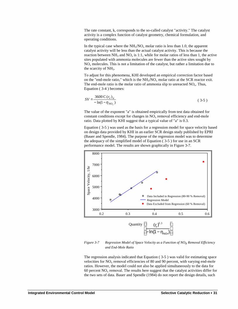
Integrated Environmental Control Model Selective Catalytic Reduction •••• 31
The rate constant, k, corresponds to the so-called catalyst "activity." The catalystactivity is a complex function of catalyst geometry, chemical formulation, andoperating conditions.
In the typical case where the NH3/NOx molar ratio is less than 1.0, the apparentcatalyst activity will be less than the actual catalyst activity. This is because thereaction between NH3 and NOx is 1:1, while for molar ratios of less than 1, the activesites populated with ammonia molecules are fewer than the active sites sought byNOx molecules. This is not a limitation of the catalyst, but rather a limitation due tothe scarcity of NH3.
To adjust for this phenomena, KHI developed an empirical correction factor basedon the "end-mole ratio," which is the NH3/NOx molar ratio at the SCR reactor exit.The end-mole ratio is the molar ratio of ammonia slip to unreacted NOx. Thus,Equation ( 3-4 ) becomes:
)1ln(
)( C 3600
xNO
aerSVη−−
= ( 3-5 )
The value of the exponent "a" is obtained empirically from test data obtained forconstant conditions except for changes in NOx removal efficiency and end-moleratio. Data plotted by KHI suggest that a typical value of "a" is 0.3.
Equation ( 3-5 ) was used as the basis for a regression model for space velocity basedon design data provided by KHI in an earlier SCR design study published by EPRI(Bauer and Spendle, 1984). The purpose of the regression model was to determinethe adequacy of the simplified model of Equation ( 3-5 ) for use in an SCRperformance model. The results are shown graphically in Figure 3-7.
0.60.50.40.30.23000
4000
5000
6000
7000
8000
Data Included in Regression (80-90 % Removal)Regression ModelData Excluded from Regression (60 % Removal)
Spa
ce V
eloc
ity, 1
/hr
Quantity
(re)0.3
− ln(1− ηNOx)
Figure 3-7 Regression Model of Space Velocity as a Function of NOx Removal Efficiency
and End-Mole Ratio
The regression analysis indicated that Equation ( 3-5 ) was valid for estimating spacevelocities for NOx removal efficiencies of 80 and 90 percent, with varying end-moleratios. However, the model could not also be applied simultaneously to the data for60 percent NOx removal. The results here suggest that the catalyst activities differ forthe two sets of data. Bauer and Spendle (1984) do not report the design details, such
32 •••• Selective Catalytic Reduction Integrated Environmental Control Model
as linear velocity; therefore it is possible that design conditions were not the same forthe two sets of data. Thus, it appears that the simple model of Equation ( 3-5 ) is areasonable basis for correcting space velocity for differences in NOx removalefficiency and end-mole ratio when all other factors are held constant.
To compare catalysts under different operating conditions, KHI suggests thefollowing model:
3.0
1
2
1
2
)1ln(
)1ln(
=
−−
m
mQWfHC rrrrrr β
ηη
( 3-6 )
From Equation ( 3-6 ), the performance of a specific catalyst may be estimated basedon ratios of key performance parameters, assuming a reference catalyst. Thisformulation suggests that space velocity can be estimated based on a referencecatalyst using multiplicative correction factors to adjust for differences in operatingconditions.
Other models are possible, such as that reported by Chen et al (1991). The NOx
removal efficiency is estimated in this model based on detailed design informationregarding the SCR catalyst, including catalyst geometry, film mass transfercoefficient, effective diffusivity, and reaction rate constant. However, data to supportthis detailed model are often not reported in published literature.
3.5.1.2. Model FormThe modeling approach adopted here is to assume a reference catalyst and to apply aseries of multiplicative correction factors to adjust space velocity for different designconditions. The general formulation is:
ii
ref fSVSV4
1=Π=
Each correction factor, fi, is a ratio that reflects the difference in space velocity fromthe reference to design conditions due to differences in certain design parameters. Ifthe reference and design conditions are the same, these correction factors have avalue of unity. A total of four correction factors have been developed, based on: (1)NOx removal efficiency; (2) end-mole ratio; (3) catalyst activity; and (4) reactiontemperature.
Default reference conditions are included in the model. The reference parametersrequired include space velocity, NOx removal efficiency, NOx inlet concentration,ammonia slip concentration, a catalyst activity curve, a catalyst life, and an operatingtemperature.
NOx Removal Efficiency
The correction factor for NOx removal efficiency is based on the model formulationsuggested by KHI. This correction factor is:
)1ln(
)1ln(1 η
η−
−== ref
effff
As the NOx removal efficiency increases, the catalyst space velocity decreases,leading to a larger catalyst volume.
For tail-end SCR, a portion of the flue gas exiting the FGD system leaks across thegas-gas heat exchanger used for flue gas reheat. Therefore, a portion of the NOx inthe flue gas will also pass across the heat exchanger and into the stack gas. Because
Integrated Environmental Control Model Selective Catalytic Reduction •••• 33
of this, the NOx removal efficiency in the SCR unit must be increased to compensatefor the NOx that bypasses the SCR system due to leakage. The required NOx removalefficiency for the SCR system is calculated based on the overall NOx removalefficiency required and the flue gas leakage rate across the gas-gas heat exchanger:
)1( i
overall
f−=
ηη
To satisfy this equation, the following constraint must be met:
1≤+ ioverall fη
This model assumes no additional NOx formation in the duct burner.
End-Mole Ratio
The correction factor for end-mole ratio is based on the design ammonia slip, thedesign inlet NOx concentration, and the design NOx removal efficiency. The end-mole ratio is given by:
)1(][
][ 3
η−=
inx
oute NO
NHr
The correction factor for end-mole ratio is given by:
3.0
,2
==
refe
er r
rff
e
Catalyst Activity
Experimental and commercial SCR operating data indicate that catalyst activitydecreases with time, due to physical and chemical changes to the catalyst aspreviously discussed. The actual rate of catalyst activity deterioration depends on theoperating conditions for the SCR reactor, and is usually not constant with time.Typically, there is an initial period of relative rapid catalyst deactivation, followedby a period of gradual activity change. A typical catalyst activity curve is shownschematically in Figure 3-8.
Schönbucher (1989) presents several curves for catalyst activity as a function of timefor high-dust and tail-end SCR systems. For wet-bottom boilers with high-dust SCR,catalyst activity loss may range from 25 to 45 percent during the first 2,000 hours ofoperation, with less rapid changes during subsequent operation. For otherapplications, such as tail-end systems on wet or dry bottom boilers, catalyst activityloss is slight (e.g., 5 percent) over 10,000 hours of operation and appears to decreaseat a relatively constant rate.
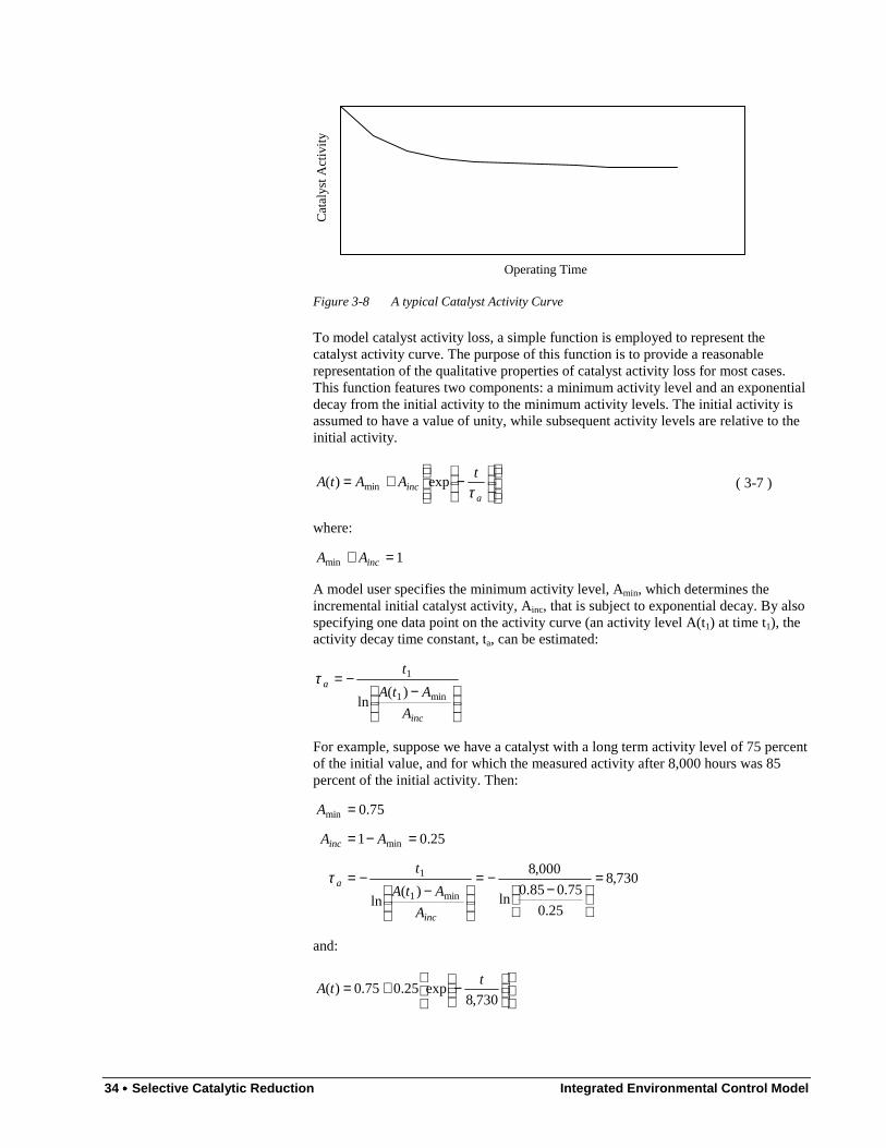
34 •••• Selective Catalytic Reduction Integrated Environmental Control Model
Operating Time
Cat
alys
t A
ctiv
ity
Figure 3-8 A typical Catalyst Activity Curve
To model catalyst activity loss, a simple function is employed to represent thecatalyst activity curve. The purpose of this function is to provide a reasonablerepresentation of the qualitative properties of catalyst activity loss for most cases.This function features two components: a minimum activity level and an exponentialdecay from the initial activity to the minimum activity levels. The initial activity isassumed to have a value of unity, while subsequent activity levels are relative to theinitial activity.
−+=
ainc
tAAtA
τexp)( min ( 3-7 )
where:
1min =+ incAA
A model user specifies the minimum activity level, Amin, which determines theincremental initial catalyst activity, Ainc, that is subject to exponential decay. By alsospecifying one data point on the activity curve (an activity level A(t1) at time t1), theactivity decay time constant, ta, can be estimated:
−−=
inc
a
A
AtA
t
min1
1
)(ln
τ
For example, suppose we have a catalyst with a long term activity level of 75 percentof the initial value, and for which the measured activity after 8,000 hours was 85percent of the initial activity. Then:
730,8
25.0
75.085.0ln
000,8
)(ln
25.01
75.0
min1
1
min
min
=
−
−=
−−=
=−=
=
inc
a
inc
A
AtA
t
AA
A
τ
and:
−+=
730,8exp25.075.0)(
ttA
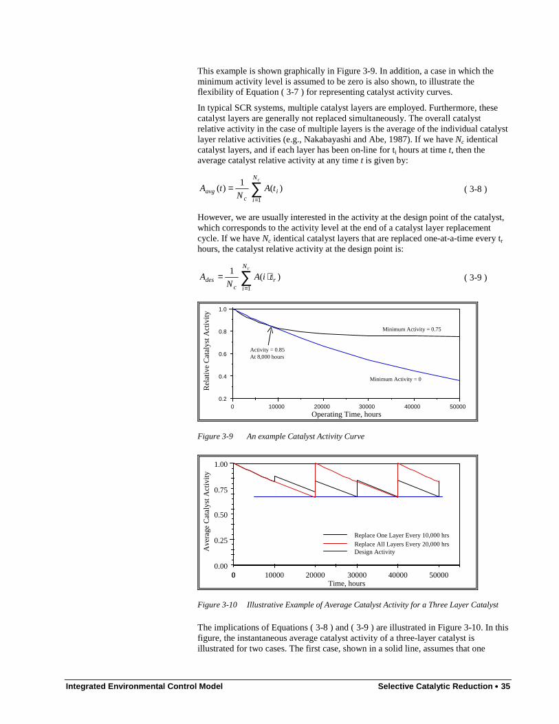
Integrated Environmental Control Model Selective Catalytic Reduction •••• 35
This example is shown graphically in Figure 3-9. In addition, a case in which theminimum activity level is assumed to be zero is also shown, to illustrate theflexibility of Equation ( 3-7 ) for representing catalyst activity curves.
In typical SCR systems, multiple catalyst layers are employed. Furthermore, thesecatalyst layers are generally not replaced simultaneously. The overall catalystrelative activity in the case of multiple layers is the average of the individual catalystlayer relative activities (e.g., Nakabayashi and Abe, 1987). If we have Nc identicalcatalyst layers, and if each layer has been on-line for ti hours at time t, then theaverage catalyst relative activity at any time t is given by:
∑=
=cN
ii
cavg tA
NtA
1
)(1
)( ( 3-8 )
However, we are usually interested in the activity at the design point of the catalyst,which corresponds to the activity level at the end of a catalyst layer replacementcycle. If we have Nc identical catalyst layers that are replaced one-at-a-time every tr
hours, the catalyst relative activity at the design point is:
∑=
⋅=cN
ir
cdes tiA
NA
1
)(1
( 3-9 )
500004000030000200001000000.2
0.4
0.6
0.8
1.0
Operating Time, hours
Rel
ativ
e C
atal
yst A
ctiv
ity
Minimum Activity = 0.75
Minimum Activity = 0
Activity = 0.85At 8,000 hours
Figure 3-9 An example Catalyst Activity Curve
5000040000300002000010000000.00
0.25
0.50
0.75
1.00
Replace One Layer Every 10,000 hrs
Design ActivityReplace All Layers Every 20,000 hrs
Time, hours
Ave
rage
Cat
alys
t Act
ivity
Figure 3-10 Illustrative Example of Average Catalyst Activity for a Three Layer Catalyst
The implications of Equations ( 3-8 ) and ( 3-9 ) are illustrated in Figure 3-10. In thisfigure, the instantaneous average catalyst activity of a three-layer catalyst isillustrated for two cases. The first case, shown in a solid line, assumes that one
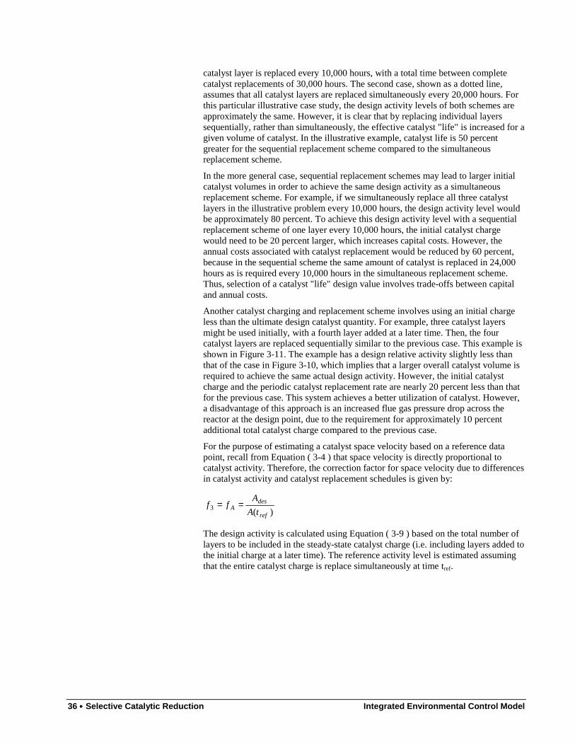
36 •••• Selective Catalytic Reduction Integrated Environmental Control Model
catalyst layer is replaced every 10,000 hours, with a total time between completecatalyst replacements of 30,000 hours. The second case, shown as a dotted line,assumes that all catalyst layers are replaced simultaneously every 20,000 hours. Forthis particular illustrative case study, the design activity levels of both schemes areapproximately the same. However, it is clear that by replacing individual layerssequentially, rather than simultaneously, the effective catalyst "life" is increased for agiven volume of catalyst. In the illustrative example, catalyst life is 50 percentgreater for the sequential replacement scheme compared to the simultaneousreplacement scheme.
In the more general case, sequential replacement schemes may lead to larger initialcatalyst volumes in order to achieve the same design activity as a simultaneousreplacement scheme. For example, if we simultaneously replace all three catalystlayers in the illustrative problem every 10,000 hours, the design activity level wouldbe approximately 80 percent. To achieve this design activity level with a sequentialreplacement scheme of one layer every 10,000 hours, the initial catalyst chargewould need to be 20 percent larger, which increases capital costs. However, theannual costs associated with catalyst replacement would be reduced by 60 percent,because in the sequential scheme the same amount of catalyst is replaced in 24,000hours as is required every 10,000 hours in the simultaneous replacement scheme.Thus, selection of a catalyst "life" design value involves trade-offs between capitaland annual costs.
Another catalyst charging and replacement scheme involves using an initial chargeless than the ultimate design catalyst quantity. For example, three catalyst layersmight be used initially, with a fourth layer added at a later time. Then, the fourcatalyst layers are replaced sequentially similar to the previous case. This example isshown in Figure 3-11. The example has a design relative activity slightly less thanthat of the case in Figure 3-10, which implies that a larger overall catalyst volume isrequired to achieve the same actual design activity. However, the initial catalystcharge and the periodic catalyst replacement rate are nearly 20 percent less than thatfor the previous case. This system achieves a better utilization of catalyst. However,a disadvantage of this approach is an increased flue gas pressure drop across thereactor at the design point, due to the requirement for approximately 10 percentadditional total catalyst charge compared to the previous case.
For the purpose of estimating a catalyst space velocity based on a reference datapoint, recall from Equation ( 3-4 ) that space velocity is directly proportional tocatalyst activity. Therefore, the correction factor for space velocity due to differencesin catalyst activity and catalyst replacement schedules is given by:
)(3ref
desA tA
Aff ==
The design activity is calculated using Equation ( 3-9 ) based on the total number oflayers to be included in the steady-state catalyst charge (i.e. including layers added tothe initial charge at a later time). The reference activity level is estimated assumingthat the entire catalyst charge is replace simultaneously at time tref.
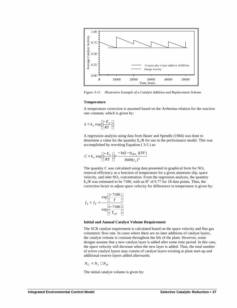
Integrated Environmental Control Model Selective Catalytic Reduction •••• 37
5000040000300002000010000000.00
0.25
0.50
0.75
1.00
3 Layers plus 1 layer added at 10,000 hrs
Design Activity
Time, hours
Ave
rage
Cat
alys
t Act
ivity
Figure 3-11 Illustrative Example of a Catalyst Addition and Replacement Scheme
Temperature
A temperature correction is assumed based on the Arrhenius relation for the reactionrate constant, which is given by:
−
=RT
Ekk a
o exp
A regression analysis using data from Bauer and Spendle (1984) was done todetermine a value for the quantity Ea/R for use in the performance model. This wasaccomplished by rewriting Equation ( 3-5 ) as:
ae
NOao
r
SV
RT
EkC x
)(3600
))(1ln(exp
η−−=
−=
The quantity C was calculated using data presented in graphical form for NOx
removal efficiency as a function of temperature for a given ammonia slip, spacevelocity, and inlet NOx concentration. From the regression analysis, the quantityEa/R was estimated to be 7180, with an R2 of 0.77 for 18 data points. Thus, thecorrection factor to adjust space velocity for differences in temperature is given by:
−
−
==
ref
T
T
Tff
7180exp
7180exp
4
Initial and Annual Catalyst Volume Requirement
The SCR catalyst requirement is calculated based on the space velocity and flue gasvolumetric flow rate. In cases where there are no later additions of catalyst layers,the catalyst volume is constant throughout the life of the plant. However, somedesigns assume that a new catalyst layer is added after some time period. In this case,the space velocity will decrease when the new layer is added. Thus, the total numberof active catalyst layers may consist of catalyst layers existing at plant start-up andadditional reserve layers added afterwards:
RIC NNN +=
The initial catalyst volume is given by:
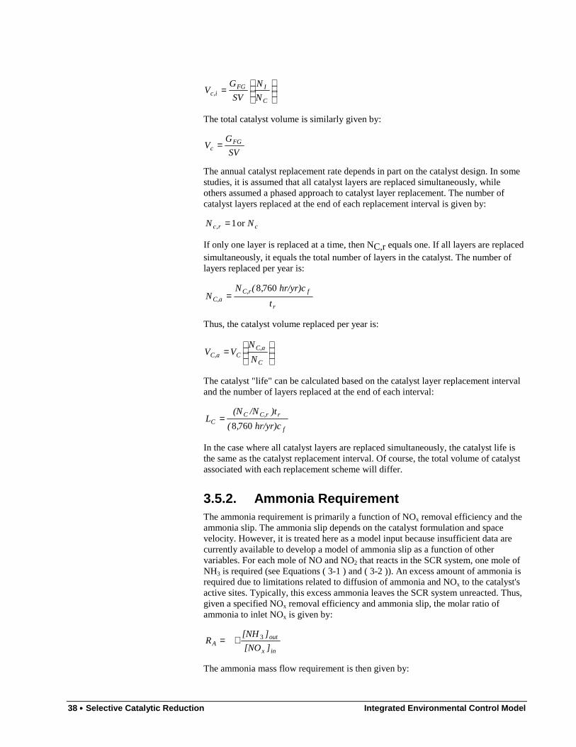
38 •••• Selective Catalytic Reduction Integrated Environmental Control Model
=
C
IFGic N
N
SV
GV ,
The total catalyst volume is similarly given by:
SV
GV FG
c =
The annual catalyst replacement rate depends in part on the catalyst design. In somestudies, it is assumed that all catalyst layers are replaced simultaneously, whileothers assumed a phased approach to catalyst layer replacement. The number ofcatalyst layers replaced at the end of each replacement interval is given by:
crc NN or 1, =
If only one layer is replaced at a time, then NC,r equals one. If all layers are replacedsimultaneously, it equals the total number of layers in the catalyst. The number oflayers replaced per year is:
r
fC,rC,a t
hr/yr)c,(NN
7608=
Thus, the catalyst volume replaced per year is:
=
C
C,aCC,a N
NVV
The catalyst "life" can be calculated based on the catalyst layer replacement intervaland the number of layers replaced at the end of each interval:
f
rC,rCC hr/yr)c,(
)t/N(NL
7608=
In the case where all catalyst layers are replaced simultaneously, the catalyst life isthe same as the catalyst replacement interval. Of course, the total volume of catalystassociated with each replacement scheme will differ.
3.5.2. Ammonia RequirementThe ammonia requirement is primarily a function of NOx removal efficiency and theammonia slip. The ammonia slip depends on the catalyst formulation and spacevelocity. However, it is treated here as a model input because insufficient data arecurrently available to develop a model of ammonia slip as a function of othervariables. For each mole of NO and NO2 that reacts in the SCR system, one mole ofNH3 is required (see Equations ( 3-1 ) and ( 3-2 )). An excess amount of ammonia isrequired due to limitations related to diffusion of ammonia and NOx to the catalyst'sactive sites. Typically, this excess ammonia leaves the SCR system unreacted. Thus,given a specified NOx removal efficiency and ammonia slip, the molar ratio ofammonia to inlet NOx is given by:
inx
outA ][NO
][NHR 3+=
The ammonia mass flow requirement is then given by:
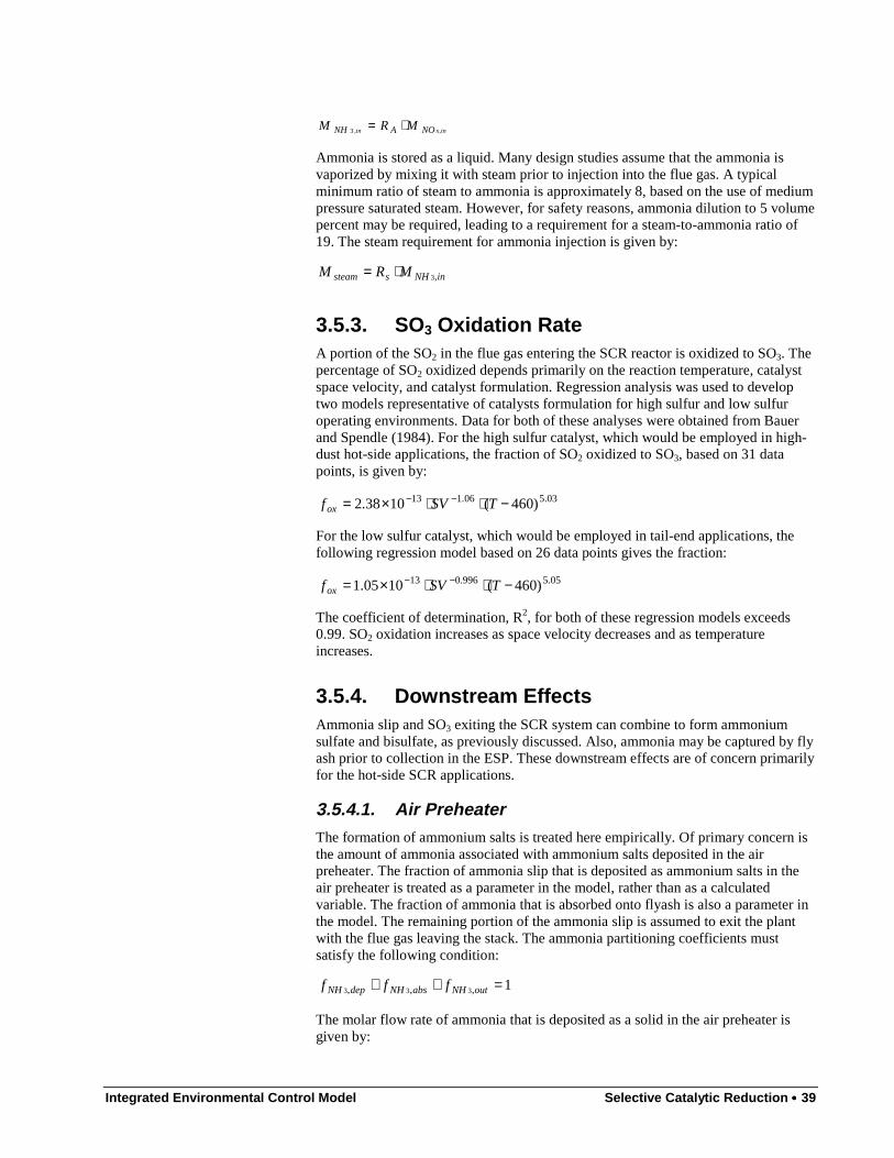
Integrated Environmental Control Model Selective Catalytic Reduction •••• 39
x,in,in NOANH MRM ⋅=3
Ammonia is stored as a liquid. Many design studies assume that the ammonia isvaporized by mixing it with steam prior to injection into the flue gas. A typicalminimum ratio of steam to ammonia is approximately 8, based on the use of mediumpressure saturated steam. However, for safety reasons, ammonia dilution to 5 volumepercent may be required, leading to a requirement for a steam-to-ammonia ratio of19. The steam requirement for ammonia injection is given by:
inNHssteam MRM ,3⋅=
3.5.3. SO3 Oxidation RateA portion of the SO2 in the flue gas entering the SCR reactor is oxidized to SO3. Thepercentage of SO2 oxidized depends primarily on the reaction temperature, catalystspace velocity, and catalyst formulation. Regression analysis was used to developtwo models representative of catalysts formulation for high sulfur and low sulfuroperating environments. Data for both of these analyses were obtained from Bauerand Spendle (1984). For the high sulfur catalyst, which would be employed in high-dust hot-side applications, the fraction of SO2 oxidized to SO3, based on 31 datapoints, is given by:
03.506.113 )460(1038.2 −⋅⋅×= −− TSVfox
For the low sulfur catalyst, which would be employed in tail-end applications, thefollowing regression model based on 26 data points gives the fraction:
05.5996.013 )460(1005.1 −⋅⋅×= −− TSVfox
The coefficient of determination, R2, for both of these regression models exceeds0.99. SO2 oxidation increases as space velocity decreases and as temperatureincreases.
3.5.4. Downstream EffectsAmmonia slip and SO3 exiting the SCR system can combine to form ammoniumsulfate and bisulfate, as previously discussed. Also, ammonia may be captured by flyash prior to collection in the ESP. These downstream effects are of concern primarilyfor the hot-side SCR applications.
3.5.4.1. Air PreheaterThe formation of ammonium salts is treated here empirically. Of primary concern isthe amount of ammonia associated with ammonium salts deposited in the airpreheater. The fraction of ammonia slip that is deposited as ammonium salts in theair preheater is treated as a parameter in the model, rather than as a calculatedvariable. The fraction of ammonia that is absorbed onto flyash is also a parameter inthe model. The remaining portion of the ammonia slip is assumed to exit the plantwith the flue gas leaving the stack. The ammonia partitioning coefficients mustsatisfy the following condition:
1,,, 333 =++ outNHabsNHdepNH fff
The molar flow rate of ammonia that is deposited as a solid in the air preheater isgiven by:
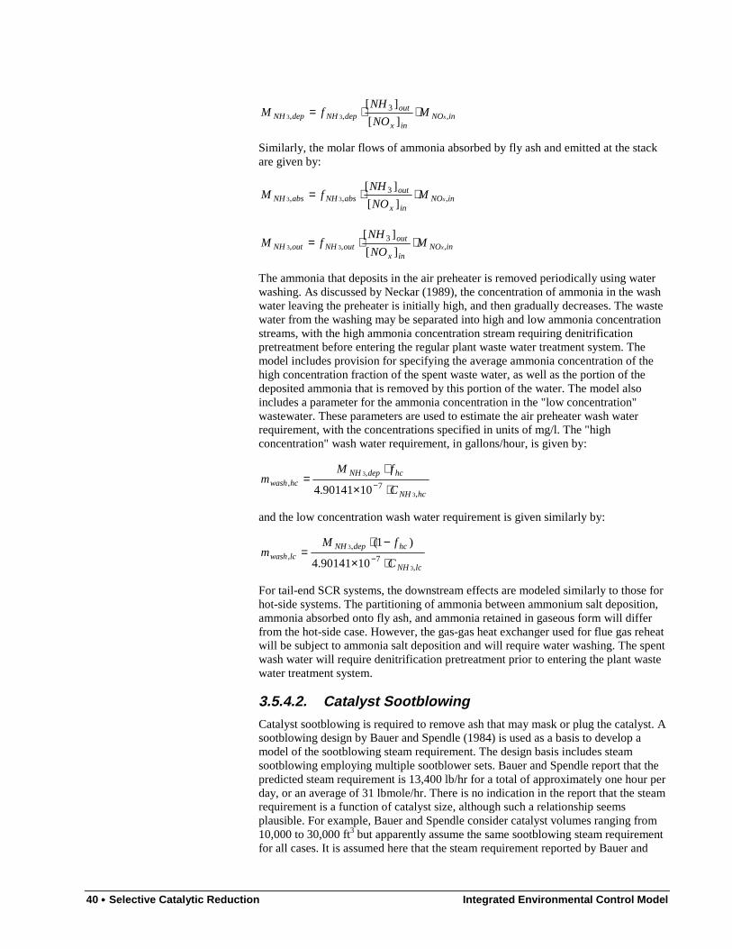
40 •••• Selective Catalytic Reduction Integrated Environmental Control Model
inNOinx
outdepNHdepNH xM
NO
NHfM ,
3,, ][
][33 ⋅⋅=
Similarly, the molar flows of ammonia absorbed by fly ash and emitted at the stackare given by:
inNOinx
outabsNHabsNH xM
NO
NHfM ,
3,, ][
][33 ⋅⋅=
inNOinx
outoutNHoutNH xM
NO
NHfM ,
3,, ][
][33 ⋅⋅=
The ammonia that deposits in the air preheater is removed periodically using waterwashing. As discussed by Neckar (1989), the concentration of ammonia in the washwater leaving the preheater is initially high, and then gradually decreases. The wastewater from the washing may be separated into high and low ammonia concentrationstreams, with the high ammonia concentration stream requiring denitrificationpretreatment before entering the regular plant waste water treatment system. Themodel includes provision for specifying the average ammonia concentration of thehigh concentration fraction of the spent waste water, as well as the portion of thedeposited ammonia that is removed by this portion of the water. The model alsoincludes a parameter for the ammonia concentration in the "low concentration"wastewater. These parameters are used to estimate the air preheater wash waterrequirement, with the concentrations specified in units of mg/l. The "highconcentration" wash water requirement, in gallons/hour, is given by:
hcNH
hcdepNHhcwash
C
fMm
,7
,,
3
3
1090141.4 ⋅×
⋅=
−
and the low concentration wash water requirement is given similarly by:
lcNH
hcdepNHlcwash
C
fMm
,7
,,
3
3
1090141.4
)1(
⋅×
−⋅=
−
For tail-end SCR systems, the downstream effects are modeled similarly to those forhot-side systems. The partitioning of ammonia between ammonium salt deposition,ammonia absorbed onto fly ash, and ammonia retained in gaseous form will differfrom the hot-side case. However, the gas-gas heat exchanger used for flue gas reheatwill be subject to ammonia salt deposition and will require water washing. The spentwash water will require denitrification pretreatment prior to entering the plant wastewater treatment system.
3.5.4.2. Catalyst SootblowingCatalyst sootblowing is required to remove ash that may mask or plug the catalyst. Asootblowing design by Bauer and Spendle (1984) is used as a basis to develop amodel of the sootblowing steam requirement. The design basis includes steamsootblowing employing multiple sootblower sets. Bauer and Spendle report that thepredicted steam requirement is 13,400 lb/hr for a total of approximately one hour perday, or an average of 31 lbmole/hr. There is no indication in the report that the steamrequirement is a function of catalyst size, although such a relationship seemsplausible. For example, Bauer and Spendle consider catalyst volumes ranging from10,000 to 30,000 ft3 but apparently assume the same sootblowing steam requirementfor all cases. It is assumed here that the steam requirement reported by Bauer and
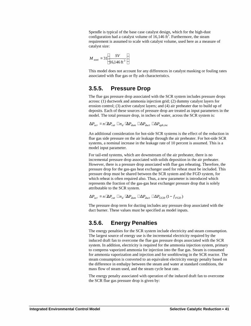
Integrated Environmental Control Model Selective Catalytic Reduction •••• 41
Spendle is typical of the base case catalyst design, which for the high-dustconfiguration had a catalyst volume of 16,146 ft3. Furthermore, the steamrequirement is assumed to scale with catalyst volume, used here as a measure ofcatalyst size:
=
3ft 146,1631
SVM soot
This model does not account for any differences in catalyst masking or fouling ratesassociated with flue gas or fly ash characteristics.
3.5.5. Pressure DropThe flue gas pressure drop associated with the SCR system includes pressure dropsacross: (1) ductwork and ammonia injection grid; (2) dummy catalyst layers forerosion control; (3) active catalyst layers; and (4) air preheater due to build up ofdeposits. Each of these sources of pressure drop are treated as input parameters in themodel. The total pressure drop, in inches of water, across the SCR system is:
incaphductdumdcatscr PPPnPnP ,∆+∆+∆⋅+∆⋅=∆
An additional consideration for hot-side SCR systems is the effect of the reduction influe gas side pressure on the air leakage through the air preheater. For hot-side SCRsystems, a nominal increase in the leakage rate of 10 percent is assumed. This is amodel input parameter.
For tail-end systems, which are downstream of the air preheater, there is noincremental pressure drop associated with solids deposition in the air preheater.However, there is a pressure drop associated with flue gas reheating. Therefore, thepressure drop for the gas-gas heat exchanger used for reheat must be included. Thispressure drop must be shared between the SCR system and the FGD system, forwhich reheat is often required also. Thus, a new parameter is introduced whichrepresents the fraction of the gas-gas heat exchanger pressure drop that is solelyattributable to the SCR system.
)1( FGDGGHductdumdcatscr fPPPnPnP −∆+∆+∆⋅+∆⋅=∆
The pressure drop term for ducting includes any pressure drop associated with theduct burner. These values must be specified as model inputs.
3.5.6. Energy PenaltiesThe energy penalties for the SCR system include electricity and steam consumption.The largest source of energy use is the incremental electricity required by theinduced draft fan to overcome the flue gas pressure drops associated with the SCRsystem. In addition, electricity is required for the ammonia injection system, primaryto compress vaporized ammonia for injection into the flue gas. Steam is consumedfor ammonia vaporization and injection and for sootblowing in the SCR reactor. Thesteam consumption is converted to an equivalent electricity energy penalty based onthe difference in enthalpy between the steam and water at standard conditions, themass flow of steam used, and the steam cycle heat rate.
The energy penalty associated with operation of the induced draft fan to overcomethe SCR flue gas pressure drop is given by:
42 •••• Selective Catalytic Reduction Integrated Environmental Control Model
scrscr,inscr,fan PGOin Hcfm
MW.E
⋅
×= −
2
610381
The fan equation here assumes a fan efficiency of 85 percent. This equation alsorepresents the energy penalty associated with a forced draft booster fan used in tail-end SCR systems.
The energy penalty associated with ammonia compression is calculated assuming a100 psi differential compression with an 85 percent compression efficiency:
inNHNHscr Mlbmole
lb
hrlb
MWE ,
5, 33
03.17
/1047.3 ⋅
⋅
×= −
The energy penalty for steam use in the SCR system is calculated based on the steammass flows, the enthalpy added to the steam by the steam cycle, and the steam cycleheat rate:
( )( )( )s
MWlbmole
lbsootsteam
steamscr HR
MME kW 000,1lb
BTU 000,118
,
)( +=
The total energy penalty for the high-dust SCR system is:
scr,steamscr,NHscr,fanscr EEEE ++= 3
For the tail-end SCR system, natural gas used to fire the duct burner represents anadditional energy loss. Natural gas is a fuel that could be used to generate electricity.Therefore, the energy penalty is calculated based upon the gross plant heat rate toestimate the equivalent electricity energy penalty associated with natural gas firing:
( )g
MWNGNG
NGscr HR
HHVmE kW 000,1
, =
The total energy penalty for the tail-end SCR system is:
NGscr,steamscr,NHscr,fanscr EEEEE +++= 3
3.5.7. Flue Gas Reheat for Tail-End SCRFor the tail-end SCR system, the temperature of the flue gas exiting the FGD systemmust be raised to the reaction temperature required by the SCR system. Furthermore,the temperature of the gas exiting the SCR system can be reduce prior to entering thestack. Therefore, a gas-gas heat exchanger (GGHX) and a duct burner are employedfor heating and cooling the flue gas, as shown in Figure 3-12.
Typically, a Ljungstrum type heat exchanger would be used for the flue gas reheatand cooling system. A portion of the higher pressure flue gas entering from the FGDsystem will leak into the flue gas stream exiting the heat exchanger to the stack.Therefore, an air leakage stream is modeled. For simplicity, it is assumed that theleakage flue gas is at the FGD system exit temperature. The flue gas leakage massflow is estimated based on a leakage fraction as follows:
oFGDlleak MfM ,=
and the flue gas fraction entering the GGHX is given by:
Integrated Environmental Control Model Selective Catalytic Reduction •••• 43
oFGDliGGH MfM ,, )1( −=
In the GGHX, the untreated flue gas is heated from the FGD exit temperature to anintermediate temperature by cooling the treated flue gas exiting the SCR system. Theheat transferred across the heat exchanger is given by:
))()(( int, FGDfgfgiGGHGGH ThThMQ −=
In the SCR computer model, the enthalpy of the flue gas is estimated usingregression models for the enthalpy of each flue gas constituent at the giventemperature.
The untreated flue gas must be heated an additional amount to reach the SCRreaction temperature. This additional heating is accomplished by use of a ductburner, which also introduces additional mass streams to the flue gas. The massbalance equation is:
airNGiDBiSCR mmmm ++= ,,
Assuming that natural gas consists only of methane, the combustion reaction is:
2222
224
)1(52.72CO
)1(52.7)1(2
NrOrOH
NrOrCH
eaea
eaea
++++
→++++

44 •••• Selective Catalytic Reduction Integrated Environmental Control Model
Flue Gasfrom
FGD System
Flue Gasto
Stack
Gas-GasHeat
Exchanger
SCR
DuctBurner
Natural Gas
Air
MDB,i Tint MSCR,o TSCR
MGGH,o Tunc
Mout Tout
MGGH,i
MFGD,o TFGD
MSCR,i TSCR
MLeak
MNGMAir
Figure 3-12 Schematic of Gas-Gas Heat Exchanger Performance Model
For each pound of methane consumed, 3.6 pounds of air are consumed atstoichiometric conditions. If excess air is also considered, the air mass flow is thengiven by:
NGeaair mrm )1(6.3 +=
The energy balance equation for the duct burner may be written as:
rNGairairNGea
NGNGNGfgiDBSCRfgiscr
HmThmr
ThmTHmThm
∆+++
+=
)()1(6.3
)()()( int,,
The heat of reaction for methane is 345,700 BTU/lbmole. In Equation ( 3-10 ), allvariables are specified except for the natural gas mass flow rate. Therefore, thisequation can be used to solve for the natural gas requirement:
rairaireaNGNG
fgiDBSCRfgiSCRNG HvThrTh
ThmThmm
∆+++
−=
)()1(6.3)(
)()( int,,( 3-10 )
In the SCR system, ammonia and steam are added to the flue gas, and the flue gascomposition changes due to chemical reactions occurring in the reactor vessel. TheSCR exit temperature is assumed to be the same as the inlet temperature. The flue
Integrated Environmental Control Model Selective Catalytic Reduction •••• 45
gas exiting the SCR unit is cooled in the GGHX. The uncorrected temperature of thetreated flue gas exiting the GGHX is estimated from the following relationship:
oGGH
GGHSCRfguncfg m
QThTh
,
)()( −=
This equation is solved using an iterative technique to determine the flue gastemperature.
The treated flue gas from the SCR system is mixed with the flue gas leaking acrossthe GGHX prior to entering the stack. The flue gas temperature entering the stack,corrected for the thermal mixing with the leakage air, is estimated using thefollowing equation:
out
FGDfgleakuncfgoGGHoutfg m
ThmThmTh
)()()(
, +=
where:
leakoGGHout mmm += ,
3.6. SCR Capital Cost ModelThe major equipment cost items for hot-side SCR systems include: (1) reactorhousing; (2) catalyst; (3) ammonia storage and injection; (4) ductwork; (5) airpreheater modifications; (6) induced draft fan modifications; (7) ash handling; and(8) water treatment. Additional costs may be incurred for flow modeling to properlydesign the ammonia injection system. For a tail-end system, there are no costsassociated with air preheater modifications or ash handling. However, there areadditional costs associated with the gas-gas heat exchanger and duct-burner used forflue gas reheat.
3.6.1. Reactor HousingA reactor housing cost model was developed by Frey (1988). This model was laterincorporated into the Integrated Air Pollution Control System (IAPCS) Version 4.0computer program (Maibodi et al., 1990). The model was based on a statisticalanalysis of data from TVA (Maxwell and Humphries, 1985). The reactor housingcosts include carbon steel reactor vessel with six inches of mineral wool insulation,vessel internals and supports, steam sootblowers, reactor crane and hoist, installationlabor, foundations, structures, piping, and electrical equipment. The costs for thereactor housing exclude catalyst. The direct capital cost for the reactor housing isgiven by:
+=
TOT
TOTR N
VDC 9.316800,145)1982(
This model was based on regression analysis of 12 data points and has a coefficientof determination (R2) of 0.998. The catalyst volume per housing ranged from 5,000to 17,000 ft3.
A similar analysis was done for data reported by EPRI (Bauer and Spendle, 1984). Atotal of 18 cost estimates were reported with catalyst volumes ranging from roughly4,000 to 14,000 ft3. However, the nature of the model was substantially differentfrom the TVA model. It appears that the TVA model is predicated on the assumption
46 •••• Selective Catalytic Reduction Integrated Environmental Control Model
of a simple linear relationship between reactor cost and catalyst volume. The EPRIdata indicate a non-linear relationship, in which larger volumes yield a substantialeconomy of scale.
A more recent EPRI study is used here as a basis for developing a reactor cost model(Robie and Ireland, 1991). A total of 14 cost estimates are reported. However, two ofthese are for oil-fired power plants. All of the remaining 12 data points are for coal-fired power plants. The two oil-fired SCR applications appear to have substantiallyhigher costs than for the coal-fired systems of similar catalyst volume; however, thebasis for the difference is not reported. Of the dozen data points for coal-firedsystems, one value is a duplicate. Therefore, 11 data points were used to develop aregression model of reactor housing cost versus total catalyst volume. The reactorhousing includes flanged gas inlet and outlet, a single vertical downflow reactor,casing, ash hoppers, structural supports for catalyst modules, rectifying plate, baffles,turning vanes, walkways, stairs, monorails, hoists, and sootblowers. The catalystvolume includes both active and spare catalyst layers.
Robie and Ireland (1991) did not report the actual catalyst volumes for all 11 datapoints used in the regression model. Therefore, the catalyst volume was estimatedbased on the reported flue gas mass flow and flue gas molecular weight (which wereused to calculated flue gas volumetric flow rate), active catalyst space velocity, andthe ratio of the number of active plus spare catalyst layers to the number of activelayers. Thus, the estimated total catalyst volume is given by:
+
=
act
spact
oact
ofg
TOT N
NN
SV
GV
where:
ofg
fgMW
m
ofg
PG
fg
fg oT R
=
The space velocity is referenced to a standard temperature and pressure, which inthis case is 32 °F and 1 atm. Therefore, the flue gas volumetric flow rate is calculatedat standard temperature and pressure. The active catalyst space velocity is adjustedbased on the ratio of total to active catalyst layers for the purpose of determining thetotal catalyst volume for the reactor housing. For the cases where the actual catalystvolumes were reported, these estimates were often in very close agreement and neverdiverged by more than five percent.
The cost data reported by Robie and Ireland (1991) are based on subcontract costsfor the process area to which additional costs have been added. These additionalcosts are not documented or discussed in the EPRI report, but appear to have beenapplied consistently for every cost reactor cost estimate. They may reflectinstallation and integration costs not covered by the subcontract costs. The multiplierfor these additional costs is a function of whether the SCR is for a new or retrofitapplication. The multipliers are substantially larger for retrofit applications,presumably reflecting site access difficulty and congestion impeding equipmentinstallation. All reactor housing costs were normalized to a new plant basis forpurposes of the regression analysis. This was done by estimating the multiplierbetween subcontractor cost and total direct cost for a new plant based on the twocase studies for a new installation. The direct costs for the remaining cases were thenestimated on a new installation basis by multiplying the subcontract costs with thenew installation direct cost factor. The relationship between direct cost and thecatalyst volume per reactor housing was evaluated using regression analysis.
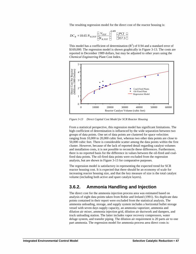
Integrated Environmental Control Model Selective Catalytic Reduction •••• 47
The resulting regression model for the direct cost of the reactor housing is:
=
3.357 65.18
489.0
,,
PCI
N
VNDC
TOTR
TOTTOTRR
This model has a coefficient of determination (R2) of 0.94 and a standard error of$169,000. The regression model is shown graphically in Figure 3-13. The costs arereported in December 1989 dollars, but may be adjusted to other years using theChemical Engineering Plant Cost Index.
60000500004000030000200001000000
1
2
3
4
5
Oil-Fired PlantCoal-Fired Plants
Regression Model
Reactor Catalyst Volume (cubic feet)
Dire
ct C
ost P
er R
eact
or(M
illio
ns 1
989
Dol
lars
)
Figure 3-13 Direct Capital Cost Model for SCR Reactor Housing
From a statistical perspective, this regression model has significant limitations. Thehigh coefficient of determination is influenced by the wide separation between twogroups of data points. One set of data points are clustered for space velocitiesranging from 10,000 to 20,000 cubic feet, whereas two other data points are close to50,000 cubic feet. There is considerable scatter among the data points within the firstcluster. However, because of the lack of reported detail regarding catalyst volumesand installation costs, it is not possible to reconcile these differences. Furthermore,there is no reported basis for the difference in values between the oil-fired and coal-fired data points. The oil-fired data points were excluded from the regressionanalysis, but are shown in Figure 3-13 for comparative purposes.
The regression model is satisfactory in representing the expected trend for SCRreactor housing cost. It is expected that there should be an economy of scale forincreasing reactor housing size, and that the key measure of size is the total catalystvolume (including both active and spare catalyst layers).
3.6.2. Ammonia Handling and InjectionThe direct cost for the ammonia injection process area was estimated based onanalysis of eight data points taken from Robie and Ireland (1991). Six duplicate datapoints contained in their report were excluded from the statistical analysis. Theammonia unloading, storage, and supply system includes a horizontal bullet storagevessel with seven days supply capacity, an ammonia vaporizer, ammonia anddilution air mixer, ammonia injection grid, dilution air ductwork and dampers, andtruck unloading station. The latter includes vapor recovery compressors, waterdeluge system, and transfer piping. The dilution air requirement is 20 parts air to onepart ammonia. The regression model for ammonia process area direct costs is:
48 •••• Selective Catalytic Reduction Integrated Environmental Control Model
=
3.357)( 8.50 482.0
,33
PCImDC iNHNH
This model has a coefficient of determination (R2) of 0.87 and a standard error of$285,000. The regression model is shown graphically in Figure 3-14. Also shown inthe figure is a regression model developed from data reported in an earlier EPRIreport (Bauer and Spendle, 1984). The newer model yields costs that are lower thanthe previous model by a factor of approximately two. The reasons for the differenceare not immediately clear. The earlier report used generally more conservativeassumptions, reflecting higher levels of uncertainty perceived at that time for thistechnology.
Like the reactor housing direct cost model, the coefficient of determination for theammonia injection system direct cost model benefits from the separation betweenclusters of data points. In this case, however, there is only one data point at the highend of the range of values for the predictive variable, ammonia flow rate. However,the model is satisfactory in reflecting economies of scale for larger sized systems.
3.6.3. DuctworkDuctwork costs are considered both for hot-side and tail-end SCR applications.
3.6.3.1. Hot-Side SCR ApplicationsFor a new hot-side SCR application, the ductwork associated with the SCR processincludes economizer bypass ducts, economizer outlet duct, SCR inlet duct, SCR inletcontrol dampers, SCR outlet duct, SCR air preheater inlet plenum, various expansionjoints in the ductwork, and dampers associated with the economizer bypass and airpreheater cross-over ducting. Of the six major case studies reported by Robie andIreland (1991), only two are for a new coal-fired power plant with hot-side SCR.Although these two case studies include five separate performance and cost estimatesbased on sensitivity analysis of key SCR performance characteristics, they arepredicated on just two flue gas flow rates. Therefore, three of these estimates areduplicates. Because only two data points are available from this study to estimateduct costs as a function of flue gas flow, regression modeling was not employed todevelop a direct cost model. Instead, a capacity-exponent model of direct cost versusflue gas volume flow rate was assumed as an appropriate function form. Thisformulation reflects the expected increase in cost that is associated with increases influe gas volume flow rates. However, it implies that duct runs would be similar fordifferently sized systems. The parameters of this model, which include amultiplicative constant and an exponential coefficient, were estimated from the twodata points. The resulting model is:
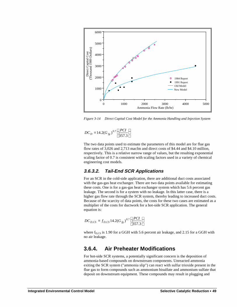
Integrated Environmental Control Model Selective Catalytic Reduction •••• 49
5000400030002000100000
1000
2000
3000
4000
5000
6000
1991 ReportOld Model
1984 Report
New Model
Ammonia Flow Rate (lb/hr)
D
irect
Cap
ital C
ost
(Tho
usan
d 19
89 D
olla
rs)
Figure 3-14 Direct Capital Cost Model for the Ammonia Handling and Injection System
=
3.357)(2.14 7.0 PCI
GDC fgD
The two data points used to estimate the parameters of this model are for flue gasflow rates of 3,026 and 2,713 macfm and direct costs of $4.44 and $4.10 million,respectively. This is a relative narrow range of values, but the resulting exponentialscaling factor of 0.7 is consistent with scaling factors used in a variety of chemicalengineering cost models.
3.6.3.2. Tail-End SCR ApplicationsFor an SCR in the cold-side application, there are additional duct costs associatedwith the gas-gas heat exchanger. There are two data points available for estimatingthese costs. One is for a gas-gas heat exchanger system which has 5.6 percent gasleakage. The second is for a system with no leakage. In this latter case, there is ahigher gas flow rate through the SCR system, thereby leading to increased duct costs.Because of the scarcity of data points, the costs for these two cases are estimated as amultiplier of the costs for ductwork for a hot-side SCR application. The generalequation is:
=
3.357)(2.14 7.0
,,PCI
GfDC fgCSDCSD
where fD,CS is 1.90 for a GGH with 5.6 percent air leakage, and 2.15 for a GGH withno air leakage.
3.6.4. Air Preheater ModificationsFor hot-side SCR systems, a potentially significant concern is the deposition ofammonia-based compounds on downstream components. Unreacted ammoniaexiting the SCR system ("ammonia slip") can react with sulfur trioxide present in theflue gas to form compounds such as ammonium bisulfate and ammonium sulfate thatdeposit on downstream equipment. These compounds may result in plugging and
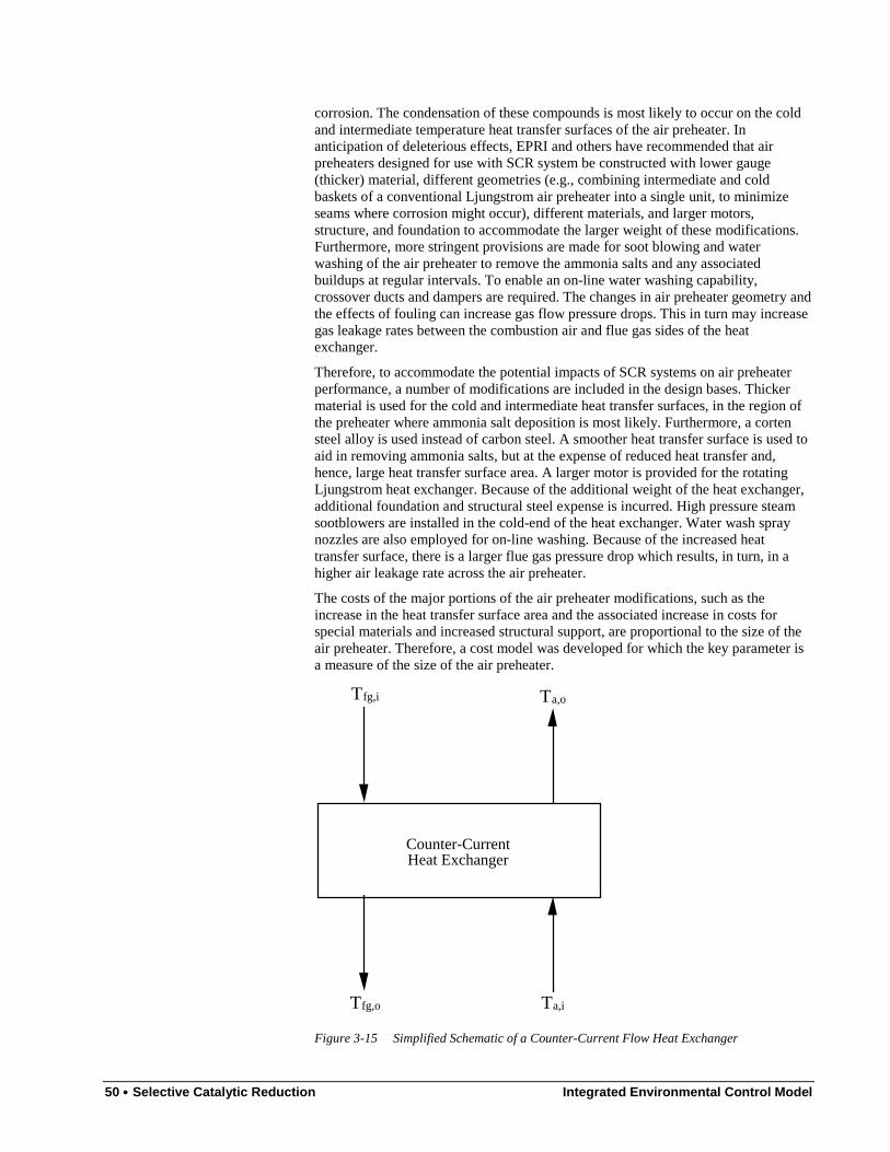
50 •••• Selective Catalytic Reduction Integrated Environmental Control Model
corrosion. The condensation of these compounds is most likely to occur on the coldand intermediate temperature heat transfer surfaces of the air preheater. Inanticipation of deleterious effects, EPRI and others have recommended that airpreheaters designed for use with SCR system be constructed with lower gauge(thicker) material, different geometries (e.g., combining intermediate and coldbaskets of a conventional Ljungstrom air preheater into a single unit, to minimizeseams where corrosion might occur), different materials, and larger motors,structure, and foundation to accommodate the larger weight of these modifications.Furthermore, more stringent provisions are made for soot blowing and waterwashing of the air preheater to remove the ammonia salts and any associatedbuildups at regular intervals. To enable an on-line water washing capability,crossover ducts and dampers are required. The changes in air preheater geometry andthe effects of fouling can increase gas flow pressure drops. This in turn may increasegas leakage rates between the combustion air and flue gas sides of the heatexchanger.
Therefore, to accommodate the potential impacts of SCR systems on air preheaterperformance, a number of modifications are included in the design bases. Thickermaterial is used for the cold and intermediate heat transfer surfaces, in the region ofthe preheater where ammonia salt deposition is most likely. Furthermore, a cortensteel alloy is used instead of carbon steel. A smoother heat transfer surface is used toaid in removing ammonia salts, but at the expense of reduced heat transfer and,hence, large heat transfer surface area. A larger motor is provided for the rotatingLjungstrom heat exchanger. Because of the additional weight of the heat exchanger,additional foundation and structural steel expense is incurred. High pressure steamsootblowers are installed in the cold-end of the heat exchanger. Water wash spraynozzles are also employed for on-line washing. Because of the increased heattransfer surface, there is a larger flue gas pressure drop which results, in turn, in ahigher air leakage rate across the air preheater.
The costs of the major portions of the air preheater modifications, such as theincrease in the heat transfer surface area and the associated increase in costs forspecial materials and increased structural support, are proportional to the size of theair preheater. Therefore, a cost model was developed for which the key parameter isa measure of the size of the air preheater.
Counter-Current Heat Exchanger
Tfg,i Ta,o
Tfg,o Ta,i
Figure 3-15 Simplified Schematic of a Counter-Current Flow Heat Exchanger
Integrated Environmental Control Model Selective Catalytic Reduction •••• 51
For a counter-current heat exchanger (see Figure 3-15), the heat transfer is given by:
aphLMaphaphaph TAUq ,∆=
where
−
−
−−−=∆
iaofg
oaifg
iaofgoaifgaphLM
TT
TT
TTTTT
,,
,,
,,,,,
ln
)()(
is the log-mean temperature difference (LMTD). The product of the universal heattransfer coefficient, U, and the heat exchanger surface area, A, is assumed here to beconstant for an air preheater before and after modification for use with SCR. Prior tomodification, the air preheater has a higher heat transfer coefficient and a lowersurface area than after modification. However, the heat exchanger is designed ineither case to accommodate the same inlet and outlet conditions and, hence, the sameLMTD. The product UA is calculated based on the known flue gas and air inlet andoutlet temperatures, the flue gas molar flow rate, and the average specific heat of fluegas. A typical value for the latter is 7.9 BTU/(lbmole-°R). Thus,
aphLM
aphaph T
qUA
,
)(∆
= ( 3-11 )
)( ,,, ifgofgfgpfgaph TTcMq −=
There are only two data points from the EPRI study which are directly relevant toestimating a reference basis for the product UA. These are the two cases involvinginstallation of a new SCR system involving Ljungstrom air preheaters (Cases 1.0 and2.0 in the EPRI report). Other cases reported are for modifications to shell and tubeheat exchangers or for retrofit modification to Ljungstrom heat exchangers.
For the first case (Case 1.0), the inlet and outlet air temperatures are not given. Theamount of heat transfer is estimated based on the flue gas cooling from 725°F to270°F. Assuming an inlet air temperature of 80°F, and accounting for air leakageacross the air preheater, the boiler air outlet temperature is estimated to beapproximately 600°F. Using these values, the LMTD is estimated to be 155°F andthe amount of heat transferred through the heat exchanger is 680 million BTU/hr.Therefore, the UA product in this case is 4.4 x 10⁶ BTU/°F. Using a similar approachfor Case 2.0 yields a UA product of 2.3 x 10⁶. In this latter case, the reported primaryair temperature (air preheater air-side outlet temperature) is inconsistent with theamount of heat transfer obtained from flue gas cooling, assuming an inlet airtemperature of 80°F. Therefore, an independently calculated value of approximately510°F was used.
The costs of air preheater modifications for the two cases are $1.37 million and$0.81 million, respectively (in December 1989 dollars). Assuming that the cost of themodification is proportional the UA product, then from these two cost estimates thefollowing capacity-exponent cost model is obtained:
=
3.357104.4N 1370
8.0
,6
,,mod,
PCI
Nx
UADC
aphT
aphTaphTaph
While this model is based on only two data points, it nonetheless appears to providea qualitatively reasonable relationship between air preheater modification costs based
52 •••• Selective Catalytic Reduction Integrated Environmental Control Model
on the size of the air preheater. The model suggests a modest economy of scale formodifications to larger air preheaters.
3.6.5. Gas-Gas Heat ExchangerThe cost model for the gas-gas heat exchanger (GGH) used for cold-side SCRapplications was developed in a manner similar to that for air preheatermodifications. The GGH is a Ljungstrom heat exchanger, and typically there is oneGGH per SCR reactor. Thus, in a typical 500 MW power plant, there would be twoGGHs.
A simplified schematic of the GGH is shown in Figure 3-16. Gas exiting the flue gasdesulfurization (FGD) system is heated by counter-current heat exchange with hightemperature gas exiting the SCR reactor. The "untreated" gas entering the SCRsystem is heated by a duct burner.
There is only one case study in the EPRI report by Robie and Ireland which dealswith a cold-side SCR. The UA product described in Equation ( 3-11 ) is assumedhere as the key measure of heat exchanger size. Based on reported gas temperaturesand flow rates, and correcting for gas leakage through the heat exchanger, the directcost model is:
=
3.357104.4 9100
8.0
,6
,,
PCI
Nx
UANDC
GGHT
GGHTGGHTGGH ( 3-12 )
This model is based on a GGH design with 5.6 percent gas leakage, on a mass basis.For a system with no leakage, multiply the cost given in Equation ( 3-12 ) by a factorof 2.4.
The cost of the duct burner is proportional to the amount of natural gas required toraise the flue gas temperature. The duct burners include combustion air fans, processcontrols, and a flame safeguard system. The capacity of the duct burners is expressedbased on the heating value of the natural gas. The direct cost is given by:
=
3.357N 90 264
6.0
DBT,,
PCIQNDC NG
DBTDB
where
610NGNG
NGHHVm
Q =
3.6.6. ID Fan and Booster Fan CostsFor a new SCR installation, the ID fans must be sized to deal with the increased fluegas pressure drop resulting from the additional ductwork and the SCR reactor.Typically, the increase in flue gas pressure drop is approximately 11 inches of water.The size of an ID fan and motor is proportional both to the flue gas flow rate and tothe pressure drop. Therefore, the cost of the ID fan modifications is assumed here tobe proportional to the difference in flue gas energy requirement necessary toovercome the flue gas pressure drop. This energy requirement is given by:
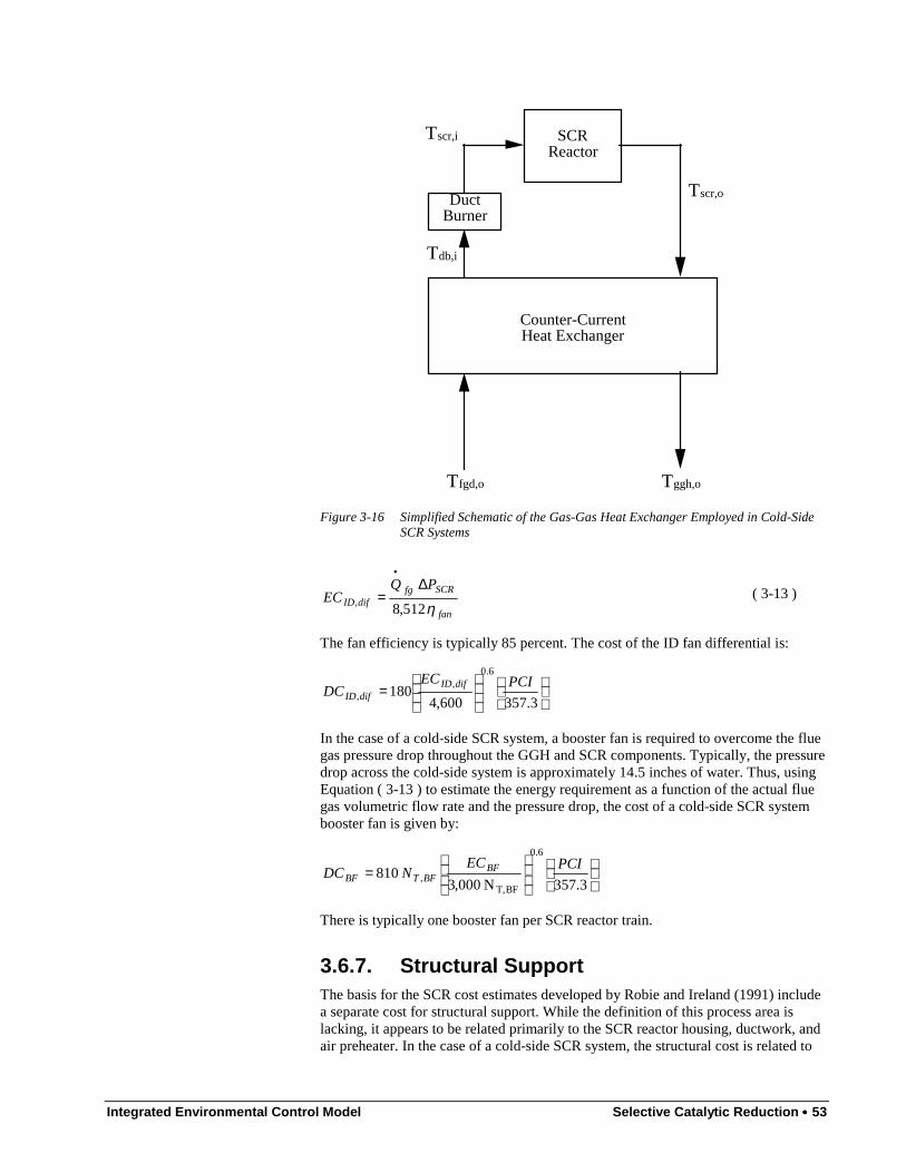
Integrated Environmental Control Model Selective Catalytic Reduction •••• 53
Counter-Current Heat Exchanger
Tscr,o
Tdb,i
Tggh,oTfgd,o
Duct Burner
SCR Reactor
Tscr,i
Figure 3-16 Simplified Schematic of the Gas-Gas Heat Exchanger Employed in Cold-SideSCR Systems
fan
SCRfgdifID
PQEC
η 512,8,
∆=
•
( 3-13 )
The fan efficiency is typically 85 percent. The cost of the ID fan differential is:
=
3.357600,4180
6.0,
,PCIEC
DCdifID
difID
In the case of a cold-side SCR system, a booster fan is required to overcome the fluegas pressure drop throughout the GGH and SCR components. Typically, the pressuredrop across the cold-side system is approximately 14.5 inches of water. Thus, usingEquation ( 3-13 ) to estimate the energy requirement as a function of the actual fluegas volumetric flow rate and the pressure drop, the cost of a cold-side SCR systembooster fan is given by:
=
3.357N 000,3 810
6.0
BFT,,
PCIECNDC BF
BFTBF
There is typically one booster fan per SCR reactor train.
3.6.7. Structural SupportThe basis for the SCR cost estimates developed by Robie and Ireland (1991) includea separate cost for structural support. While the definition of this process area islacking, it appears to be related primarily to the SCR reactor housing, ductwork, andair preheater. In the case of a cold-side SCR system, the structural cost is related to
54 •••• Selective Catalytic Reduction Integrated Environmental Control Model
the gas-gas heat exchanger, rather than the air preheater. As part of the data analysis,the structural cost was expressed as a percentage of the direct costs for the reactorhousing, ductwork, and air preheater modifications for hot-side applications, and as apercentage of the direct costs for the reactor housing, ductwork, and gas-gas heatexchanger costs for cold-side applications. Of the 14 data points from the EPRIstudy, 12 of them yielded structural costs as a relatively narrow range of percentagesof the appropriate direct costs. The mean value was 18.7 percent, with a range from16.2 to 20.8 percent and a standard deviation of 1.4 percent. For one retrofit casewith a high site congestion, the structural costs were 50 percent of the other selecteddirect costs. For a new SCR hot-side application, the structural costs are estimatedas:
)( APHDRss DCDCDCfDC ++=
and for a cold-side application the structural costs are estimated as:
)( GGHDRss DCDCDCfDC ++=
where fs has a mean value of 0.187. For a retrofit application, a value of fs of as highas 0.5 may be appropriate.
3.6.8. Miscellaneous Other Direct Capital CostsOther capital costs may be incurred for ash handling addition, water treatmentaddition, and flow modeling for a hot-side SCR system. For a cold-side system, costsare incurred for water treatment and flow modeling.
Flow modeling costs are similar for all systems and typically represent a flat fee fordesigning the ammonia injection system to assure proper mixing of ammonia andflue gas. The value used in the EPRI study was $100,000.
Ash handling addition is required for hot side systems to remove ash deposited in thebottom of the SCR reactor to existing ash piping or to an ash silo. This cost is smallcompared to the costs of reactors, ammonia injection, heat exchangers, and fans.Here, it is assumed to have a value of approximately $150,000 for a 550 MW powerplant.
For hot-side applications, there is additional waste water burden associated withsoot-blowing and water washing in the SCR system. In the cold-side system,additional equipment is required to collect GGH wastewater. For hot-side systems,the additional cost associated with water treatment are less than $150,000. For cold-side systems, they are approximately $500,000. These numbers are representative ofa typical 550 MW power plant.
The direct cost for miscellaneous expenses of flow modeling, ash handling addition,and water treatment addition for a hot-side SCR system are:
+=
3.357
550300100
6.0PCIMW
DC emisc
For a cold-side SCR system, the direct cost is:
+=
3.357
550650100
6.0
,PCIMW
DC eCSmisc

Integrated Environmental Control Model Selective Catalytic Reduction •••• 55
3.6.9. Total Direct CostThe total direct cost is the sum of all of the direct costs. The cost of the initialcatalyst charge is also included here in the total direct cost, because it is such a largeand integral part of the SCR system. One component of the direct cost not estimatedin any of the above sections is the cost of general facilities associated with the SCRprocess area. Based on the estimates reported by Robie and Ireland, it appears thatgeneral facilities cost is approximately 4 percent of the sum of all other direct costs.The total direct cost for the hot-side SCR system is therefore:
++= ∑
=
7
1
)1(i
icatactGFHS DCUCVfTDC
where there are seven direct cost components (reactor housing, ammonia injection,ductwork, air preheater modifications, ID fan differential, structural, andmiscellaneous).
For a cold-side system, the total direct cost is given by:
++= ∑
=
8
1
)1(i
icatactGFCS DCUCVfTDC
where there are eight direct cost components (reactor housing, ammonia injectionsystem, ductwork, gas-gas heat exchanger, duct burner, booster fan, structural, andmiscellaneous).
3.6.10. Other Capital CostsOther capital costs include various indirect capital costs, as well as preproductioncosts associated with startup and inventory costs associated with providing initialstocks of chemicals and fuels.
Engineering and home office fees are typically estimated as a percentage of the totaldirect cost. In this case, a value of 10 percent is assumed as the default.
TDCfC EHOEHO =
Project contingency costs are also approximately 10 percent, as assumed by Robieand Ireland. Usually, project contingency is assigned as a multiplier of the totaldirect cost (e.g., EPRI, 1986). For example:
TDCfC ojCojC PrPr =
Process contingency costs are typically evaluated separately for each process area.The total process contingency is given by:
∑=i
iojCocC DCfC PrPr
Typical values of the process contingency are: five percent for reactor, catalyst,structural support, and fans; ten percent for ammonia storage, ductwork, air preheatermodifications, and gas-gas heat exchanger; fifteen percent for water treatmentaddition, and twenty percent for ash handling addition.
The total plant cost, or overnight construction cost, is given by:
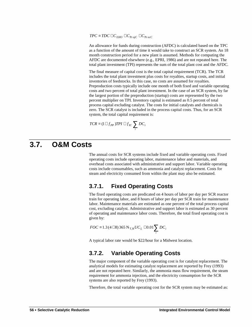
56 •••• Selective Catalytic Reduction Integrated Environmental Control Model
ocCojCEHO CCCTDCTPC PrPr +++=
An allowance for funds during construction (AFDC) is calculated based on the TPCas a function of the amount of time it would take to construct an SCR system. An 18month construction period for a new plant is assumed. Methods for computing theAFDC are documented elsewhere (e.g., EPRI, 1986) and are not repeated here. Thetotal plant investment (TPI) represents the sum of the total plant cost and the AFDC.
The final measure of capital cost is the total capital requirement (TCR). The TCRincludes the total plant investment plus costs for royalties, startup costs, and initialinventories of feedstocks. In this case, no costs are assumed for royalties.Preproduction costs typically include one month of both fixed and variable operatingcosts and two percent of total plant investment. In the case of an SCR system, by farthe largest portion of the preproduction (startup) costs are represented by the twopercent multiplier on TPI. Inventory capital is estimated as 0.5 percent of totalprocess capital excluding catalyst. The costs for initial catalysts and chemicals iszero. The SCR catalyst is included in the process capital costs. Thus, for an SCRsystem, the total capital requirement is:
∑++=i
iICPP DCfTPIfTCR )1(
3.7. O&M CostsThe annual costs for SCR systems include fixed and variable operating costs. Fixedoperating costs include operating labor, maintenance labor and materials, andoverhead costs associated with administrative and support labor. Variable operatingcosts include consumables, such as ammonia and catalyst replacement. Costs forsteam and electricity consumed from within the plant may also be estimated.
3.7.1. Fixed Operating CostsThe fixed operating costs are predicated on 4 hours of labor per day per SCR reactortrain for operating labor, and 8 hours of labor per day per SCR train for maintenancelabor. Maintenance materials are estimated as one percent of the total process capitalcost, excluding catalyst. Administrative and support labor is estimated as 30 percentof operating and maintenance labor costs. Therefore, the total fixed operating cost isgiven by:
∑++=i
iL DCUCFOC 01.0N 365 )84( 3.1 RT,
A typical labor rate would be $22/hour for a Midwest location.
3.7.2. Variable Operating CostsThe major component of the variable operating cost is for catalyst replacement. Theanalytical models for estimating catalyst replacement are reported by Frey (1993)and are not repeated here. Similarly, the ammonia mass flow requirement, the steamrequirement for ammonia injection, and the electricity consumption for the SCRsystems are also reported by Frey (1993).
Therefore, the total variable operating cost for the SCR system may be estimated as:

Integrated Environmental Control Model Selective Catalytic Reduction •••• 57
+
+
+= elecscrsteam
steamNH
iANHfcataC UCEUC
MUC
McUCVVOC
000,1
18
6.117760,8 3
3 ,,,
The unit cost for catalyst is highly variable. Robie and Ireland (1991) used a value of$660/ft3, but noted that at the time of their study, catalyst costs in Europe were aslow as $330/ft3. The unit cost of ammonia is typically $150/ton. The unit cost ofsteam is approximately $3.00/1,000 lb. The cost of power is often assumed to be 5cents per kWh.
3.8. Nomenclature
3.8.1. Performance Models
3.8.1.1. English Letter Symbolsa = Constant
Ac = Catalyst area, ft2
Amin = Minimum catalyst activity level
Ainc = Incremental catalyst activity subject to exponential decay (1-Amin)
AV = Area velocity, ft/hr
cf = Annual plant capacity factor, fraction of year
C = Constant representing catalyst activity for a given operatingcondition (e.g., temperature, inlet NOx concentration) withNH3/NOx ratio equal to 1.0
Ci = Vector of concentrations of trace species in stream i, ppmw
CNH3,hc = Concentration of ammonia in "high concentration" washwater, mg/l
CNH3,k = Concentration of ammonia in "low concentration" wash water,mg/l
Cr = Ratio of catalyst activities for two catalysts.
Ea = Activation energy
Ei = Energy penalty for system i, MW
fFGD = Fraction of gas-gas heat exchanger pressure drop that isnormally associated with FGD flue gas reheat.
fhc = Fraction of ammonia deposited on air preheater surfacesremoved in high concentration wash water.
fi = Generic correction factor
F1 = Fraction of flue gas exiting FGD system that leaks across gas-gas heat exchanger in tail-end SCR system
fNH3= Fraction of ammonia slip partitioned to fate i (e.g.,
"dep"=deposition on air preheater surfaces, "abs"=absorbed byflyash, "out"=emitted with flue gas)
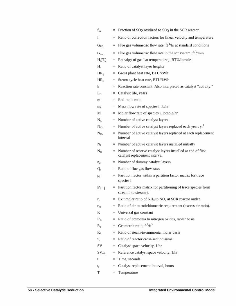
58 •••• Selective Catalytic Reduction Integrated Environmental Control Model
fox = Fraction of SO2 oxidized to SO3 in the SCR reactor.
fr = Ratio of correction factors for linear velocity and temperature
GFG = Flue gas volumetric flow rate, ft3/hr at standard conditions
Gscr = Flue gas volumetric flow rate in the scr system, ft3/min
Hi(Tj) = Enthalpy of gas i at temperature j, BTU/lbmole
Hr = Ratio of catalyst layer heights
HRg = Gross plant heat rate, BTU/kWh
HRs = Steam cycle heat rate, BTU/kWh
k = Reaction rate constant. Also interpreted as catalyst "activity."
LC = Catalyst life, years
m = End-mole ratio
mi = Mass flow rate of species i, lb/hr
Mi = Molar flow rate of species i, lbmole/hr
NC = Number of active catalyst layers
NC,a = Number of active catalyst layers replaced each year, yr1
NC,r = Number of active catalyst layers replaced at each replacementinterval
NI = Number of active catalyst layers installed initially
NR = Number of reserve catalyst layers installed at end of firstcatalyst replacement interval
nd = Number of dummy catalyst layers
Qr = Ratio of flue gas flow rates
pi = Partition factor within a partition factor matrix for tracespecies i
Pi � j = Partition factor matrix for partitioning of trace species fromstream i to stream j.
re = Exit molar ratio of NH3 to NOx at SCR reactor outlet.
rea = Ratio of air to stoichiometric requirement (excess air ratio).
R = Universal gas constant
RA = Ratio of ammonia to nitrogen oxides, molar basis
Rg = Geometric ratio, ft2/ft3
RS = Ratio of steam-to-ammonia, molar basis
Sr = Ratio of reactor cross-section areas
SV = Catalyst space velocity, 1/hr
SVref = Reference catalyst space velocity, 1/hr
t = Time, seconds
tr = Catalyst replacement interval, hours
T = Temperature
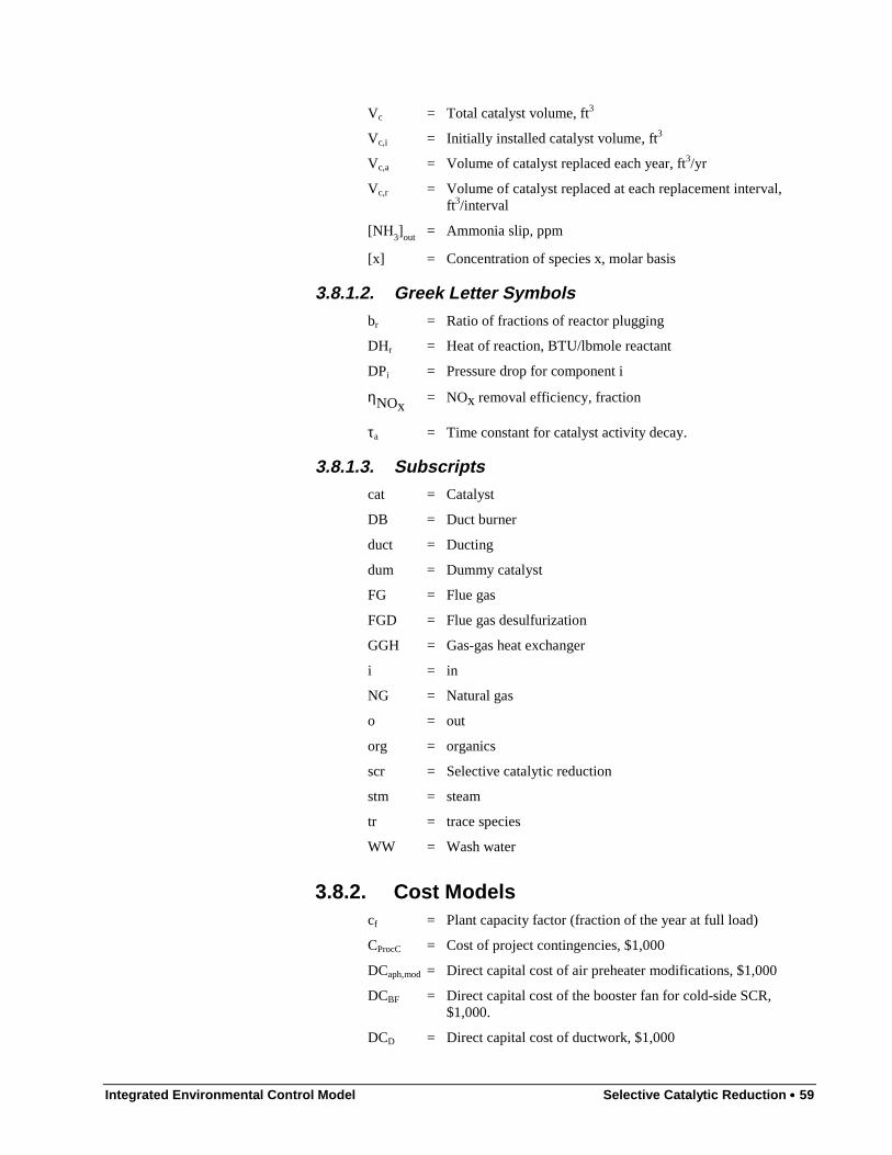
Integrated Environmental Control Model Selective Catalytic Reduction •••• 59
Vc = Total catalyst volume, ft3
Vc,i = Initially installed catalyst volume, ft3
Vc,a = Volume of catalyst replaced each year, ft3/yr
Vc,r = Volume of catalyst replaced at each replacement interval,ft3/interval
[NH3]out = Ammonia slip, ppm
[x] = Concentration of species x, molar basis
3.8.1.2. Greek Letter Symbolsbr = Ratio of fractions of reactor plugging
DHr = Heat of reaction, BTU/lbmole reactant
DPi = Pressure drop for component i
ηNOx = NOx removal efficiency, fraction
τa = Time constant for catalyst activity decay.
3.8.1.3. Subscriptscat = Catalyst
DB = Duct burner
duct = Ducting
dum = Dummy catalyst
FG = Flue gas
FGD = Flue gas desulfurization
GGH = Gas-gas heat exchanger
i = in
NG = Natural gas
o = out
org = organics
scr = Selective catalytic reduction
stm = steam
tr = trace species
WW = Wash water
3.8.2. Cost Modelscf = Plant capacity factor (fraction of the year at full load)
CProcC = Cost of project contingencies, $1,000
DCaph,mod = Direct capital cost of air preheater modifications, $1,000
DCBF = Direct capital cost of the booster fan for cold-side SCR,$1,000.
DCD = Direct capital cost of ductwork, $1,000
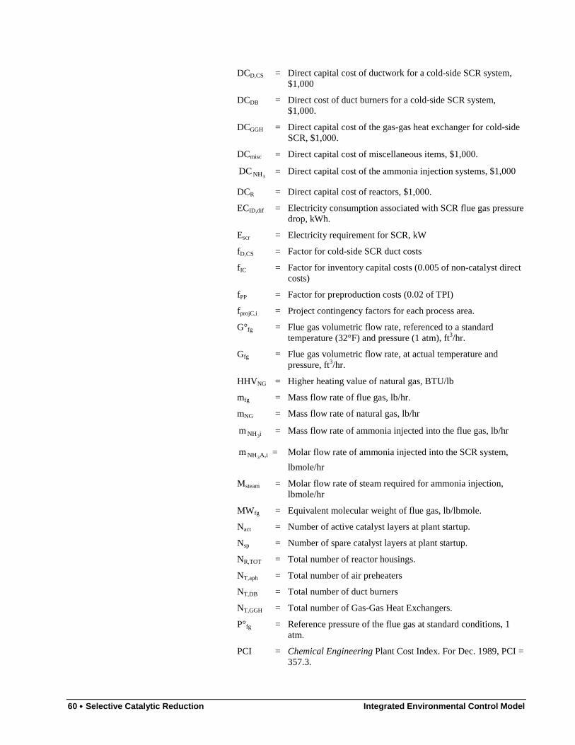
60 •••• Selective Catalytic Reduction Integrated Environmental Control Model
DCD,CS = Direct capital cost of ductwork for a cold-side SCR system,$1,000
DCDB = Direct cost of duct burners for a cold-side SCR system,$1,000.
DCGGH = Direct capital cost of the gas-gas heat exchanger for cold-sideSCR, $1,000.
DCmisc = Direct capital cost of miscellaneous items, $1,000.
3NHDC = Direct capital cost of the ammonia injection systems, $1,000
DCR = Direct capital cost of reactors, $1,000.
ECID,dif = Electricity consumption associated with SCR flue gas pressuredrop, kWh.
Escr = Electricity requirement for SCR, kW
fD,CS = Factor for cold-side SCR duct costs
fIC = Factor for inventory capital costs (0.005 of non-catalyst directcosts)
fPP = Factor for preproduction costs (0.02 of TPI)
fprojC,i = Project contingency factors for each process area.
G°fg = Flue gas volumetric flow rate, referenced to a standardtemperature (32°F) and pressure (1 atm), ft3/hr.
Gfg = Flue gas volumetric flow rate, at actual temperature andpressure, ft3/hr.
HHVNG = Higher heating value of natural gas, BTU/lb
mfg = Mass flow rate of flue gas, lb/hr.
mNG = Mass flow rate of natural gas, lb/hr
iNH3m = Mass flow rate of ammonia injected into the flue gas, lb/hr
iA,NH3m = Molar flow rate of ammonia injected into the SCR system,
lbmole/hr
Msteam = Molar flow rate of steam required for ammonia injection,lbmole/hr
MWfg = Equivalent molecular weight of flue gas, lb/lbmole.
Nact = Number of active catalyst layers at plant startup.
Nsp = Number of spare catalyst layers at plant startup.
NR,TOT = Total number of reactor housings.
NT,aph = Total number of air preheaters
NT,DB = Total number of duct burners
NT,GGH = Total number of Gas-Gas Heat Exchangers.
P°fg = Reference pressure of the flue gas at standard conditions, 1atm.
PCI = Chemical Engineering Plant Cost Index. For Dec. 1989, PCI =357.3.
Integrated Environmental Control Model Selective Catalytic Reduction •••• 61
fgQ•
= Flue gas volumetric flow rate, actual ft3/min.
QNG = Heating value of natural gas used in duct burners, BTU/hr.
R = Ideal Gas Constant, 0.730 (fte3 atm)/(lbmole °R).
SV°act = Active catalyst space velocity, referenced to a flue gastemperature of 32°F, 1/hr.
Ta,i = Temperature of air entering a heat exchanger, °R.
Ta,o = Temperature of air exiting a heat exchanger, °R.
T°fg = Reference temperature of the flue gas at standard conditions,32°F.
Tfg,i = Temperature of flue gas entering a heat exchanger, °R.
Tfg,o = Temperature of flue gas exiting a heat exchanger, °R.
UA = Product of universal heat transfer coefficient and heatexchanger surface area, BTU/°R
UCcat = Unit cost of catalyst, $/ft3.
UCelec = Unit cost of electricity, $/kWh
UCL = Unit cost of labor, $/hour
3NHUC = Unit cost of ammonia, $/ton
UCsteam = Unit cost of steam, $/1,000 lb
VC,A = Volume of catalyst replaced annually, ft3/yr.
VTOT = Total volume of the catalyst, including active and spare layers,ft3.
3.9. ReferencesAnderson, C. M., and J. A. Billings. "Simple Calculation Measures NH3 Slip forCogeneration Units," Power Engineering, April 1991, pp. 42-44.
Balling, L., and D. Hein. "DeNOx Catalytic Converters for Various Types ofFurnaces and Fuels--Development, Testing, and Operation," in 1989 Symposium onStationary Combustion Nitrogen Oxide Control, Volume 2. Electric Power ResearchInstitute. Palo Alto, California. Report No. GS-6423. July 1989. pp. 7A-27 to 7A-40.
Bauer, T.K., and R.G. Spendle (1984), "Selective Catalytic Reduction for Coal-FiredPower Plants: Feasibility and Economics," CS-3603, Electric Power ResearchInstitute, Palo Alto, CA, October.
Behrens, E. S., S. Ikeda, T. Yamashita, G. Mittelbach, and M. Yanai. "SCROperating Experience on Coal-Fired Boilers and Recent Progress," presented at the1991 Symposium on Stationary Combustion Nitrogen Oxide Control, Washington,DC, March 25-28, 1991.
Chen, J. P., M. A. Buzanowski, R.T. Yang, and J.E. Chicanowicz, "Deactivation ofthe Vanadia Catalyst in the Selective Catalytic Reduction Process," JAWMA40(10):1403-1409 (December 1990).

62 •••• Selective Catalytic Reduction Integrated Environmental Control Model
Chen, J., R.T. Yang, and J.E. Chicanowicz. "Poisoning of SCR Catalysts," presentedat the 1991 Symposium on Stationary Combustion Nitrogen Oxide Control,Washington, DC, March 25-28, 1991.
CMU (1993), "Development of the Integrated Environmental Control Model:Performance Models of Selective Catalytic Reduction (SCR) NOx Control Systems,"Quarterly Progress Report prepared by Carnegie Mellon University for U.S.Department of Energy, June 1993.
EPA. Integrated Air Pollution Control System, Version 4.0, Volume 2: TechnicalDocumentation Manual.
EPRI (1986). TAG - Technical Assessment Guide. Vol 1. P-4463-SR. Electric PowerResearch Institute. Palo Alto, CA. December.
Fickett, K.L., "Clean Coal-NOx for the 21st Century: Managing Permit Risk withSelective Catalytic Reduction (SCR) Technology," Paper 43a presented at theAIChE 1993 Summer National Meeting, Seattle, WA, August 14-18, 1993.
Flora, H., J. Barkely, G.Janik, B. Marker, and J.E. Chicanowicz, "Status of 1 MWSCR Pilot Plant Tests at Tennessee Valley Authority and New York State Electricand Gas," presented at the 1991 Symposium on Stationary Combustion NitrogenOxide Control, Washington, DC, March 25-28, 1991.
Frey, H. C. (1988), "Selective Catalytic Reduction Cost Algorithm for the AdvancedUtility Simulation Model", Technical Memorandum to J. A. Martinez, RadianCorporation, July 8.
Gouker, T.R., and C.P. Brundrett. "SCR Catalyst Developments for the U.S.Market," presented at the 1991 Symposium on Stationary Combustion NitrogenOxide Control, Washington, DC, March 25-28, 1991.
Johnson, K.L., G.S. Shareef, and P.A. May. Evaluation of Oil-Fired Gas TurbineSelective Catalytic Reduction (SCR) NOx Control. Prepared by Radian Corporationfor the Gas Research Institute and Electric Power Research Institute. EPRI ReportNo. GS-7056. December 1990.
Koppius-Odink, J.M., et al. "The First DE-NOx Installation in the Netherlands: ADemonstration Project at Epon-Nijmegen Power Station," in 1989 Symposium onStationary Combustion Nitrogen Oxide Control, Volume 2. Electric Power ResearchInstitute. Palo Alto, California. Report No. GS-6423. July 1989. pp. 6A-57 to 6A-83.
Kuroda, H., et al. "Recent Developments in the SCR System and Its OperationalExperience," in 1989 Symposium on Stationary Combustion Nitrogen OxideControl, Volume 2. Electric Power Research Institute. Palo Alto, California. ReportNo. GS-6423. July 1989. pp. 6A-39 to 6A-55.
Lowe, P.A., W. Ellison, and M. Perlsweig (1991), "Understanding the German andJapanese Coal-Fired SCR Experience," presented at the 1991 Symposium onStationary Combustion Nitrogen Oxide Control, Washington, DC, March 25-28,1991.
Maibodi, M., A. L. Blackard, and R. J. Page (1990), "Integrated Air PollutionControl System Version 4.0, Volume 2: Technical Documentation Manual,"Prepared by Radian Corporation for U.S. Environmental Protection Agency, EPA-600/7-90-022b, December.
Maier, H., and P. Dahl, "Operating Experience With Tail-End and High-Dust Denox-Technics at the Power Plant of Heilbronn," presented at the 1991 Symposium onStationary Combustion Nitrogen Oxide Control, Washington, DC, March 25-28,1991.

Integrated Environmental Control Model Selective Catalytic Reduction •••• 63
Maxwell, J. D., and L.R. Humphries (1985), "Economics of Nitrogen Oxides, SulfurOxides, and Ash Control Systems for Coal-Fired Utility Power Plants," Prepared forU.S. Environmental Protection Agency, EPA-600/7-85-006, February.
May, P.A., L.M. Campbell, and K.L. Johnson. "Environmental and EconomicEvaluation of Gas Turbine SCR NOx Control," presented at the 1991 Symposium onStationary Combustion Nitrogen Oxide Control, Washington, DC, March 25-28,1991.
Mori, T., and N. Shimizu. "Operating Experience of SCR Systems at EPDC's Coal-Fired Power Station," in 1989 Symposium on Stationary Combustion NitrogenOxide Control, Volume 2. Electric Power Research Institute. Palo Alto, California.Report No. GS-6423. July 1989. pp. 6A-85 to 6A-104.
Nakabayashi, Y., and R. Abe, "Current Status of SCR in Japan," in 1987 Symposiumon Stationary Combustion Nitrogen Oxide Control, Volume 2. Electric PowerResearch Institute. Palo Alto, California. Report No. CS-5361. August 1987. pp. 25-1 to 25-29
Necker, I.P. "Experience Gained by Neckarwerke from Operation of SCR DeNOxUnits," in 1989 Symposium on Stationary Combustion Nitrogen Oxide Control,Volume 2. Electric Power Research Institute. Palo Alto, California. Report No. GS-6423. July 1989. pp. 6A-19 to 6A-38.
Novak, M., and H.G. Rych. "Design and Operation of the SCR-Type NOx ReductionPlants at the Dürnrohr Power Station in Austria," in 1989 Symposium on StationaryCombustion Nitrogen Oxide Control, Volume 2. Electric Power Research Institute.Palo Alto, California. Report No. GS-6423. July 1989. pp. 7A-1 to 7A-26.
Offen, G.R., D.Eskanazi, M.W. McElroy, and J.S. Maulbetsch, "StationaryCombustion NOx Control," JAPCA 37(7):864-871.
Robie, C.P., and P.A. Ireland (1991), "Technical Feasibility and Cost of SelectiveCatalytic Reduction (SCR) NOx Control," GS-7266, Prepared by United Engineersand Constructors, Inc. for the Electric Power Research Institute, Palo Alto, CA, May.
Robie, C.P., P.A. Ireland, and J.E. Chicanowicz. "Technical Feasibility andEconomics of SCR NOx Control in Utility Applications," in 1989 Symposium onStationary Combustion Nitrogen Oxide Control, Volume 2. Electric Power ResearchInstitute. Palo Alto, California. Report No. GS-6423. July 1989. pp. 6A-105 to 6A-124.
Robie, C.P., P.A. Ireland, and J.E. Chicanowicz. "Technical Feasibility and Cost ofSCR for U.S. Utility Application," presented at the 1991 Symposium on StationaryCombustion Nitrogen Oxide Control, Washington, DC, March 25-28, 1991.
Rubin, E.S., J.S. Salmento, J.G. Barrett, C.N. Bloyd, and H.C. Frey, Modeling andAssessment of Advanced Processes for Integrated Environmental Control of Coal-Fired Power Plants, prepared by Carnegie-Mellon University for the U.S.Department of Energy, Pittsburgh, Pennsylvania, NTIS DE86014713, July 1986.
Rubin, E.S., J.S. Salmento, H.C. Frey, A. Abu-Baker, and M. Berkenpas, Modelingof Integrated Environmental Control Systems for Coal-Fired Power Plants, FinalReport, Prepared by Carnegie-Mellon University for the U.S. Department of Energy,Pittsburgh, Pennsylvania, DOE Contract No. DE-AC22-87PC79864, April 1991,214p.
Schönbucher, B. "Reduction of Nitrogen Oxides from Coal-Fired Power Plants byUsing the SCR Process: Experiences in the Federal Republic of Germany with Pilotand Commercial Scale DeNOx Plants," in 1989 Symposium on Stationary

64 •••• Selective Catalytic Reduction Integrated Environmental Control Model
Combustion Nitrogen Oxide Control, Volume 2. Electric Power Research Institute.Palo Alto, California. Report No. GS-6423. July 1989. pp. 6A-1 to 6A-17.
Shiomoto, G.H., and L.J. Muzio, "Selective Catalytic Reduction for Coal-FiredPower Plants: Pilot Plant Results," Prepared by KVB, Inc. for the Electric PowerResearch Institute, Palo Alto, CA, Report No. CS-4386, April 1986.
U.S. Department of Energy, "Clean Coal Technology Demonstration Program:Program Update 1991", DOE/FE-0247P, February 1992.

Integrated Environmental Control Model Electrostatic Precipitator •••• 65
4. Electrostatic Precipitator
4.1. IntroductionThis chapter describes the development of analytical models for the performance andcosts of high-performance particulate control technologies, focusing on electrostaticprecipitators. Special attention is paid to developing models which can be used toestimate costs for systems whose performance is up to a factor of three below thepresent NSPS standards of 0.03 lb/MMBtu. Typically, the cost models relate thecapital costs and the operating and maintenance (O&M) costs to process parametersand the costs of labor and materials. The capital cost models are anchored to a basecapital cost for a specific size unit and adjusted according to the actual or designparameters. The performance models are constructed to estimate the processparameters for a desired level of emissions control. The primary motivation for thesemodels is to estimate the costs of complying with environmental standards on a basiswhich reflects recent advances in control technology. Finally, we incorporate theuncertainties in various process parameters and inputs costs so as to allow a morerational and robust basis for comparing different technologies.
The development of the performance and cost models for electrostatic precipitators isdiscussed, followed by a numerical example which illustrates the use of these newmodels.
4.2. BackgroundESPs have long been the work horse of particulate collection at coal-fired powerplants. A large number of electrostatic precipitators were installed in power plants inthe 1950's and 60's when 30-40% stack plume opacity was considered adequate.However, these ESP's were inadequate as the regulations in the 70's forced utilities tomove to low sulfur coals with high resistivity ash. As a result it was not unusual forcoal-fired power plants to suffer reductions in capacity due to excessive stackopacity. However, since the 80s due to a tremendous improvement in the technology,ESPs have demonstrated performance that is at least as good as modern day fabricfilters. Older vintage ESPs (of 50s and 60s) performed at 0.1 lbs/MBtu for highsulfur coals. The ESPs in the 80s are almost twice the size1 of the older ones (400-450 SCA today) and have demonstrated outlet emissions consistently well below 0.1lbs/MBtu. In the utility industry (Kumar & Feldman, 1994), (Mastropietro, 1994a),the improved performance of ESPs has reduced the emissions of particulate matterfrom 0.1 lbs/MBtu to 0.01 lbs/MBtu over the last 15 years. In applications in thechemical industry (Kumar & Feldman, 1994), ESPs with SCA of 550-650 have been
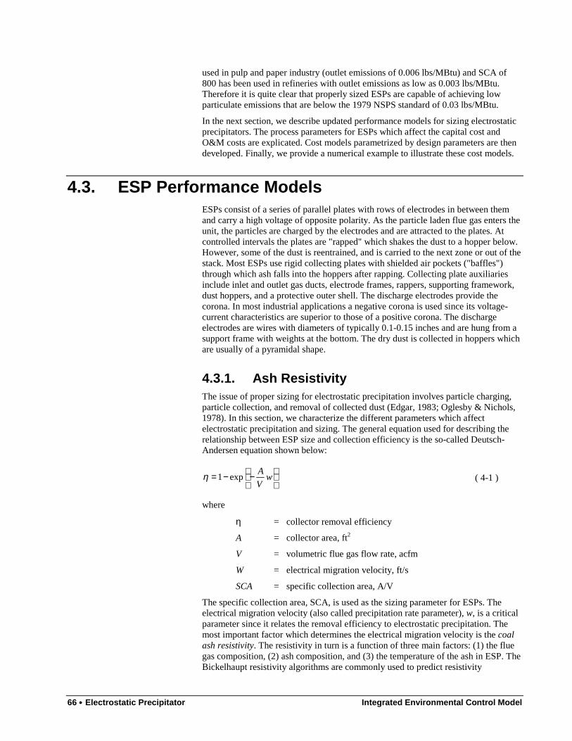
66 •••• Electrostatic Precipitator Integrated Environmental Control Model
used in pulp and paper industry (outlet emissions of 0.006 lbs/MBtu) and SCA of800 has been used in refineries with outlet emissions as low as 0.003 lbs/MBtu.Therefore it is quite clear that properly sized ESPs are capable of achieving lowparticulate emissions that are below the 1979 NSPS standard of 0.03 lbs/MBtu.
In the next section, we describe updated performance models for sizing electrostaticprecipitators. The process parameters for ESPs which affect the capital cost andO&M costs are explicated. Cost models parametrized by design parameters are thendeveloped. Finally, we provide a numerical example to illustrate these cost models.
4.3. ESP Performance ModelsESPs consist of a series of parallel plates with rows of electrodes in between themand carry a high voltage of opposite polarity. As the particle laden flue gas enters theunit, the particles are charged by the electrodes and are attracted to the plates. Atcontrolled intervals the plates are "rapped" which shakes the dust to a hopper below.However, some of the dust is reentrained, and is carried to the next zone or out of thestack. Most ESPs use rigid collecting plates with shielded air pockets ("baffles")through which ash falls into the hoppers after rapping. Collecting plate auxiliariesinclude inlet and outlet gas ducts, electrode frames, rappers, supporting framework,dust hoppers, and a protective outer shell. The discharge electrodes provide thecorona. In most industrial applications a negative corona is used since its voltage-current characteristics are superior to those of a positive corona. The dischargeelectrodes are wires with diameters of typically 0.1-0.15 inches and are hung from asupport frame with weights at the bottom. The dry dust is collected in hoppers whichare usually of a pyramidal shape.
4.3.1. Ash ResistivityThe issue of proper sizing for electrostatic precipitation involves particle charging,particle collection, and removal of collected dust (Edgar, 1983; Oglesby & Nichols,1978). In this section, we characterize the different parameters which affectelectrostatic precipitation and sizing. The general equation used for describing therelationship between ESP size and collection efficiency is the so-called Deutsch-Andersen equation shown below:
−−= w
V
A exp1η ( 4-1 )
where
η = collector removal efficiency
A = collector area, ft2
V = volumetric flue gas flow rate, acfm
W = electrical migration velocity, ft/s
SCA = specific collection area, A/V
The specific collection area, SCA, is used as the sizing parameter for ESPs. Theelectrical migration velocity (also called precipitation rate parameter), w, is a criticalparameter since it relates the removal efficiency to electrostatic precipitation. Themost important factor which determines the electrical migration velocity is the coalash resistivity. The resistivity in turn is a function of three main factors: (1) the fluegas composition, (2) ash composition, and (3) the temperature of the ash in ESP. TheBickelhaupt resistivity algorithms are commonly used to predict resistivity

Integrated Environmental Control Model Electrostatic Precipitator •••• 67
(Bickelhaupt, 1986; Bickelhaupt & Altman, 1984). The algorithms are based on aresistivity-reciprocal absolute temperature curve which is derived from three separateeffects discussed below.
1. Volume resistivity, ρv, can be described as the resistivity of flyash
excluding the influence of flue gas composition. Ash composition,temperature, and physical characteristics of the particulate layerprincipally affect it.
2. Surface resistivity, ρs, results from the interaction of ash surface with
adsorbed water vapor. Ash composition, gas temperature, gas moistureconcentration and physical characteristics of ash affect it.
3. Acid resistivity, ρa, represents the conduction mechanism associated
with adsorbed sulfuric acid vapor. It is affected by the sulfur content ofcoal.
The overall resistivity (ρvsa) is calculated by treating these individual resistances in
parallel and is provided in the equation below:
sasvva
svavsa pppppp
pppp
×+×+×××
= ( 4-2 )
We have implemented this algorithm for calculating coal ash resistivity in IECM andis shown in “Analytica Model Code for Ash Resistivity” on page 76. However, thereis some discrepancy in the predictions of this model and values used in industrialpractice especially for western coals (Mastropietro, 1994b; Sloat, 1994). As shown inTable 4-1, we introduce correction factors (Mastropietro, 1994b) for the Bickelhauptmodels where appropriate. “Coal and Ash Analysis” on page 81 provides an ultimateanalysis and the coal ash composition for each coal type (based on literature).
Table 4-1 Coal Resistivity
Coal Type * IndustryExperience
Bickelhauptalgorithm
Correctionfactors
App.MS E8-E10 1.3E9 1
WPCU E9 - E10 7.6E10 1
Ill#6 E8 - E10 3E8 1
NDL E8 - E10 3E8 1
WPRB (low)
(high)
E9 - E11
E13
9E10 (low)
2E12(high)
1 (low)
10 (high)
App.LS E12 1.2E12 1
* The coals used for comparison have the following attributes or properties:
App.MS = Appalachian Medium Sulfur (12.7 KBtu/lb. 2% S, 8% ash)
App.LS = Appalachian Low Sulfur (12.2 KBtu/lb, 0.5% S, 11.4% ash)
WPCU = Wasatch Plateau (Central Utah) (11.24 KBtu/lb, 0.6% S, 11%ash)
Ill#6 = East Central Illinois #6 (10.1 KBtu/lb, 4% S, 16% ash)
NDL = North Dakota Lignite (6.6 KBtu/lb, 0.7% S, 7.8 % ash)

68 •••• Electrostatic Precipitator Integrated Environmental Control Model
WPRB = Wyoming Powder River Basin, (8.0 KBtu/lb, 0.5% S, 6.4%ash) the Na2O content in ash varies 0.1-0.5%, 0.5%corresponds to low resistivity and 0.1% to high resistivity
4.3.2. Effective Migration VelocityThe next step in developing performance models involves correlating the totalresistivity ρsva to the electrical migration velocity w. It is possible to develop a
theoretical model which relates w to resistivity, which involves solving for theelectric field and current density in the gas space between the collecting plates. Thisrequires numerically solving for a set of partial differential equations which describethe electric field in between the plates (McLean, 1988; Oglesby & Nichols, 1978;White, 1977). Various computer-based theoretical models have been developedwhich represent in greater detail the electrical properties of ash and its particle sizedistribution (Lawless & Altman, 1989; Lawless & Plaks, 1989). However in practice,such idealized calculations often do not match experimental data well due to non-uniformities in gas flow distribution, gas sneakage, and rapping reentrainment.Moreover, it is desirable, especially in preliminary design, to have models that arerelatively simple to use. In this report, we derive correlations between w andresistivity ρsva by deriving "effective" values for w corresponding to empirical data
for SCA values for different coals and different emission limits. A modified versionof the Deutsch equation, discussed below, is used to derive the effective values for w.These values are then correlated to the coal ash resistivity derived from the correctedBickelhaupt algorithms.
The Deutsch-Anderson Equation (see ( 4-1 )) is accurate only up to 95% removalefficiencies. Various empirical models have been developed to describe the "tailingoff" of the efficiency curve at higher efficiencies (η > 95%). One such empiricallybased performance model that has found widespread use and is able to effectivelydescribe the efficiency curve for high A/V values was developed by White (White,1977) and is provided in the following equation:
k
kwV
A
−−= exp1η ( 4-3 )
This equation is the so-called modified Deutsch equation. Typically, a value of6.0≈k (Mastropietro, 1994b) is used in industrial practice today. In Table 4-2,
typical SCA values for different removal efficiencies and coals are provided. Themodified Deutsch equation ( 4-3 ) is used to derive the values for precipitation rateparameter wk (column 5) corresponding to two sets of empirical SCA values. It isimportant to remember that when we use the modified-Deutsch equation ( 4-3 ), therate parameter wk ceases to have a physical interpretation (such as precipitationvelocity for Equation ( 4-2 )) and only provides a way to parameterize the effect ofresistivity.

Integrated Environmental Control Model Electrostatic Precipitator •••• 69
Table 4-2 Estimation of wk
Coal η %η %η %η % SCA1 wk1 SCA2 wk
2 wk(aver)
App. MS
98
99.4
99.8
205
295
415
0.0474
0.0515
0.0506
175
270
370
0.0555
0.0563
0.0568
0.053
WPCU
98.7
99.6
99.87
255
385
520
0.0453
0.0448
0.0452
285
425
575
0.0406
0.0406
0.0409
0.043
Ill #6
99.2
99.76
99.92
220
320
425
0.0627
0.0625
0.0622
230
335
440
0.06
0.0597
0.06
0.061
NDL
98.9
99.68
99.89
220
310
420
0.056
0.0556
0.0583
230
335
440
0.0535
0.0515
0.0556
0.055
WPRB
(low resist)
98
99.5
99.8
280
405
550
0.0347
0.0398
0.0382
0.037
WPRB
(high resist)
98
99.5
99.8
540
835
1055
0.018
0.0193
0.0199
0.019
App.LS
98.65
99.6
99.87
320
490
665
0.0356
0.0352
0.0353
355
540
735
0.0321
0.0319
0.032
0.034
1 SCA values are based on typical values suggested by vendors (Gaikwad & Sloat,1992)2 SCA values used by Research-Cottrell (Mastropietro, 1994b)
The effective values calculated for wk and the corresponding resistivities for eachcoal type (shown in Table 4-2) are summarized in Table 4-3.
Table 4-3 Summary of Resistivity and wk
Coal Resistivity
(ohm-cm)
Wk
App.MS 1.3E9 0.053
WPCU 7.6E10 0.043
Ill #6 3E8 0.0612
NDL 3E8 0.055
WPRB (low) 9E10 0.037
WPRB (high) 2E13 0.019
App.LS 1.2E12 0.034
We now derive a regression model to develop a functional relation betweenresistivity and the parameter wk. We find that a log-linear relationship (resistivity on
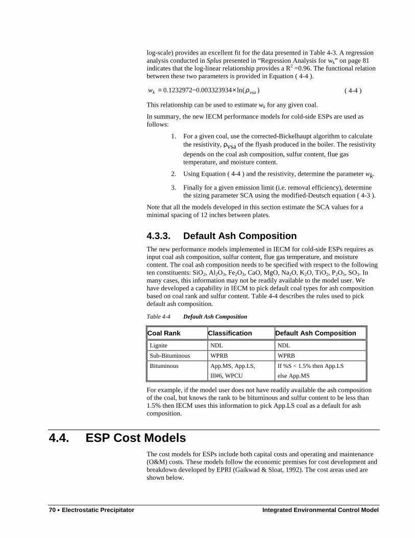
70 •••• Electrostatic Precipitator Integrated Environmental Control Model
log-scale) provides an excellent fit for the data presented in Table 4-3. A regressionanalysis conducted in Splus presented in “Regression Analysis for wk” on page 81indicates that the log-linear relationship provides a R2 =0.96. The functional relationbetween these two parameters is provided in Equation ( 4-4 ).
)(ln003323934.01232972.0 vsakw ρ×−= ( 4-4 )
This relationship can be used to estimate wk for any given coal.
In summary, the new IECM performance models for cold-side ESPs are used asfollows:
1. For a given coal, use the corrected-Bickelhaupt algorithm to calculatethe resistivity, ρvsa of the flyash produced in the boiler. The resistivity
depends on the coal ash composition, sulfur content, flue gastemperature, and moisture content.
2. Using Equation ( 4-4 ) and the resistivity, determine the parameter wk.
3. Finally for a given emission limit (i.e. removal efficiency), determinethe sizing parameter SCA using the modified-Deutsch equation ( 4-3 ).
Note that all the models developed in this section estimate the SCA values for aminimal spacing of 12 inches between plates.
4.3.3. Default Ash CompositionThe new performance models implemented in IECM for cold-side ESPs requires asinput coal ash composition, sulfur content, flue gas temperature, and moisturecontent. The coal ash composition needs to be specified with respect to the followingten constituents: SiO2, Al2O3, Fe2O3, CaO, MgO, Na2O, K2O, TiO2, P2O5, SO3. Inmany cases, this information may not be readily available to the model user. Wehave developed a capability in IECM to pick default coal types for ash compositionbased on coal rank and sulfur content. Table 4-4 describes the rules used to pickdefault ash composition.
Table 4-4 Default Ash Composition
Coal Rank Classification Default Ash Composition
Lignite NDL NDL
Sub-Bituminous WPRB WPRB
Bituminous App.MS, App.LS,
Ill#6, WPCU
If %S < 1.5% then App.LS
else App.MS
For example, if the model user does not have readily available the ash compositionof the coal, but knows the rank to be bituminous and sulfur content to be less than1.5% then IECM uses this information to pick App.LS coal as a default for ashcomposition.
4.4. ESP Cost ModelsThe cost models for ESPs include both capital costs and operating and maintenance(O&M) costs. These models follow the economic premises for cost development andbreakdown developed by EPRI (Gaikwad & Sloat, 1992). The cost areas used areshown below.
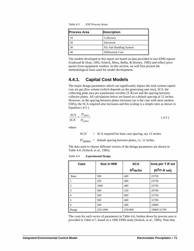
Integrated Environmental Control Model Electrostatic Precipitator •••• 71
Table 4-5 ESP Process Areas
Process Area Description
10 Collectors
20 Ductwork
30 Fly Ash Handling System
40 Differential Cost
The models developed in this report are based on data provided in two EPRI reports(Gaikwad & Sloat, 1992; Scheck, Mora, Belba, & Horney, 1985) and reflect pricequotes from equipment vendors. In this section, we will first present themethodological basis used for model development.
4.4.1. Capital Cost ModelsThe major design parameters which can significantly impact the total system capitalcost are gas flow volume (which depends on the generating unit size), SCA, thecollecting plate area per transformer-rectifier (T-R) set and the spacing betweencollector plates. All calculations below are based on a default spacing of 12 inches.However, as the spacing between plates increases (as is the case with most modernESPs), the SCA required also increases and this scaling is a simple ratio as shown inEquation ( 4-5 ).
//plates
plates
D
D
SCA
SCA = ( 4-5 )
where
SCA/ = SCA required for base case spacing, say 12 inches
D/plates = default spacing between plates, i.e. 12 inches
The data used to choose different vectors of the design parameters are shown inTable 4-6. (Scheck, et al., 1985).
Table 4-6 Experimental Design
Case Size in MW SCA
ft2/acfm
Area per T-R set
(ft2/T-R set)
Base 500 400 23750
1 250 400 23750
2 1000 400 23750
3 500 250 29700
4 500 800 23750
5 500 400 31700
6 500 400 19000
Range 250-1000 250-800 19000-31700
The costs for each vector of parameters in Table 4-6, broken down by process area isprovided in Table 4-7, based on a 1985 EPRI study (Scheck, et al., 1985). Note that
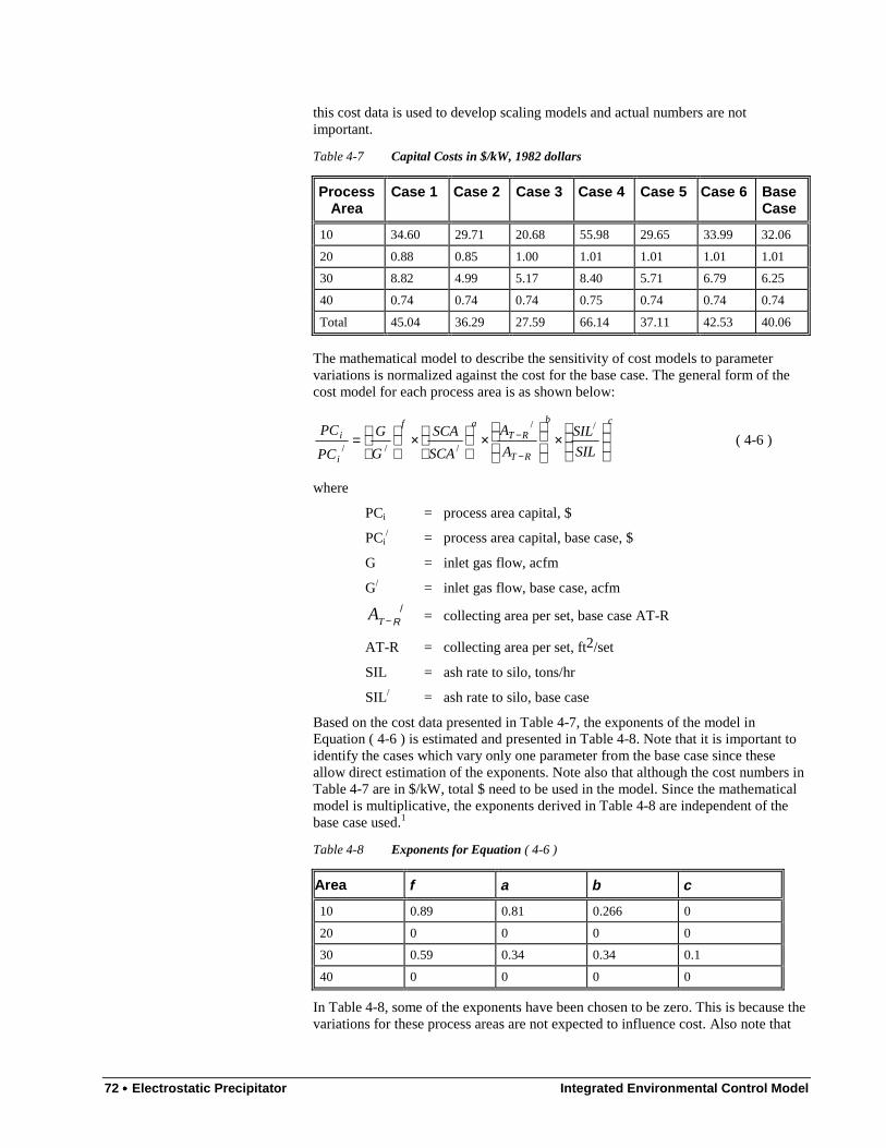
72 •••• Electrostatic Precipitator Integrated Environmental Control Model
this cost data is used to develop scaling models and actual numbers are notimportant.
Table 4-7 Capital Costs in $/kW, 1982 dollars
ProcessArea
Case 1 Case 2 Case 3 Case 4 Case 5 Case 6 BaseCase
10 34.60 29.71 20.68 55.98 29.65 33.99 32.06
20 0.88 0.85 1.00 1.01 1.01 1.01 1.01
30 8.82 4.99 5.17 8.40 5.71 6.79 6.25
40 0.74 0.74 0.74 0.75 0.74 0.74 0.74
Total 45.04 36.29 27.59 66.14 37.11 42.53 40.06
The mathematical model to describe the sensitivity of cost models to parametervariations is normalized against the cost for the base case. The general form of thecost model for each process area is as shown below:
cb
RT
RTaf
i
i
SIL
SIL
A
A
SCA
SCA
G
G
PC
PC
×
×
×
=
−
−//
///( 4-6 )
where
PCi = process area capital, $
PCi/ = process area capital, base case, $
G = inlet gas flow, acfm
G/ = inlet gas flow, base case, acfm
AT− R/
= collecting area per set, base case AT-R
AT-R = collecting area per set, ft2/set
SIL = ash rate to silo, tons/hr
SIL/ = ash rate to silo, base case
Based on the cost data presented in Table 4-7, the exponents of the model inEquation ( 4-6 ) is estimated and presented in Table 4-8. Note that it is important toidentify the cases which vary only one parameter from the base case since theseallow direct estimation of the exponents. Note also that although the cost numbers inTable 4-7 are in $/kW, total $ need to be used in the model. Since the mathematicalmodel is multiplicative, the exponents derived in Table 4-8 are independent of thebase case used.1
Table 4-8 Exponents for Equation ( 4-6 )
Area f a b c
10 0.89 0.81 0.266 0
20 0 0 0 0
30 0.59 0.34 0.34 0.1
40 0 0 0 0
In Table 4-8, some of the exponents have been chosen to be zero. This is because thevariations for these process areas are not expected to influence cost. Also note that
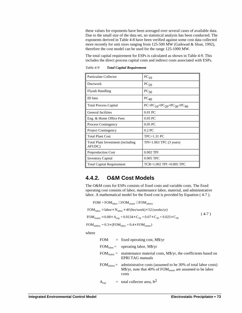
Integrated Environmental Control Model Electrostatic Precipitator •••• 73
these values for exponents have been averaged over several cases of available data.Due to the small size of the data set, no statistical analysis has been conducted. Theexponents derived in Table 4-8 have been verified against some cost data collectedmore recently for unit sizes ranging from 125-500 MW (Gaikwad & Sloat, 1992),therefore the cost model can be used for the range 125-1000 MW.
The total capital requirement for ESPs is calculated as shown in Table 4-9. Thisincludes the direct process capital costs and indirect costs associated with ESPs.
Table 4-9 Total Capital Requirement
Particulate Collector PC10
Ductwork PC20
Flyash Handling PC30
ID fans PC40
Total Process Capital PC=PC10+PC20+PC30+PC40
General facilities 0.01 PC
Eng. & Home Office Fees 0.05 PC
Process Contingency 0.05 PC
Project Contingency 0.2 PC
Total Plant Cost TPC=1.31 PC
Total Plant Investment (includingAFUDC)
TPI=1.063 TPC (3 years)
Preproduction Cost 0.002 TPI
Inventory Capital 0.005 TPC
Total Capital Requirement TCR=1.002 TPI +0.005 TPC
4.4.2. O&M Cost ModelsThe O&M costs for ESPs consists of fixed costs and variable costs. The fixedoperating cost consists of labor, maintenance labor, material, and administrativelabor. A mathematical model for the fixed cost is provided by Equation ( 4-7 ).
)FOM 0.4 + (FOM0.3 =FOM
C0.025 + C0.07 + C0.0134 + A0.08 FOM
(weeks/yr) 52 (hrs/week) 40 N labor FOM
FOMFOMFOM =FOM
maintlaboradmin
403020espmaint
laborlabor
adminmaintlabor
××
××××=
×××=
++
( 4-7 )
where
FOM = fixed operating cost, M$/yr
FOMlabor = operating labor, M$/yr
FOMmaint. = maintenance material costs, M$/yr, the coefficients based onEPRI TAG manuals
FOMadmin = administrative costs (assumed to be 30% of total labor costs)M$/yr, note that 40% of FOMmaint. are assumed to be laborcosts
Aesp = total collector area, ft2

74 •••• Electrostatic Precipitator Integrated Environmental Control Model
labor = labor rate, $/hour
Nlabor = number of laborers at 40 hrs/week
Ci = capital for process area i (20,30,40)
Notice that the model has been developed analytically except that the dependence onunit size is based on process area costs.
Table 4-10 O&M costs in 1990 $/kW-yr
O&M 125 MW 250 MW 500 MW
Ash 2.23 2.23 2.23
Power 1.41 1.31 1.23
Table 4-10 provides the variation in fixed and variable costs as a function of plantsize (assuming a capacity factor of 65%). The variable cost includes the power costand ash disposal cost. The ash disposal cost is proportional to the ash generated. Thepower costs are calculated based on the T-R set power and the other auxiliary powerrequirements. The variable operating cost is given by
}{8760 =VOM
8760= VOM
VOM + VOM =VOM
//
//
power
ash
powerash
q
power
ash
G
GAR
G
GTRCcf
TC cf
×+
××××
×××( 4-8 )
where G, G/ are as before and
VOM = variable operating costs, M$/yr
VOMash = ash disposal costs, M$/yr
VOMpower = power costs (includes T-R power and auxiliary power due topressure drop etc), M$/yr
cf = capacity factor
T = ash disposal rate, tons/hr
Cash = ash disposal cost, $/ton, (default 10.24)
Cpower = power cost, cents/KWh, (5.54 c/kWh)
TR/ = T-R set power as a function of efficiency, as shown inEquation ( 4-9 )
AR/ = Auxiliary power other than T-R set (includes energy penaltyfor pressure drop), 522 kW base case
q = 0.65, exponent derived from data in Table 4-9
Notice that Equation ( 4-8 ) is such that the base case cannot be changedarbitrarily . The T-R set power consumption is a function of removal efficiency andis given by Equation ( 4-9 ).
r
ATR
−×=
1001/ η
( 4-9 )
where

Integrated Environmental Control Model Electrostatic Precipitator •••• 75
A = constant in T-R set power
η = particle removal efficiency
r = exponent in Equation ( 4-9 )
The values of constants A, r were determined based on quotes from various vendors(Gaikwad & Sloat, 1992), and are provided in Table 4-11.
Table 4-11 Parameters for Equation ( 4-9 )
Coal A r
App.MS 78 -0.375
WPCU 81 -0.371
Ill.#6 95 -0.34
NDL 108 -0.353
WPRB (low) 102 -0.36
WPRB (high) 57 -0.39
App.LS 67 -0.40
4.4.3. A Numerical ExampleWe will use a base case of unit size 250 MW (0.95 Macfm), with a SCA of400ft2/acfm, 23750 ft2/per T-R set, using Appalachian Medium Sulfur coal (ash content8%, ash rate to silo =10.44 tons/hr). We estimate the cost of a unit with the followingdesign parameters:
Size = 500 MW net(1.9 Macfm), SCA = 415 ft2/acfm,
30000 ft2/per T-R set, Capacity factor =65%,
Emission limit = 0.01 lb/MMBtu (99.86%), Ash disposal rate = 10.441 tons/hr
4.4.3.1. Capital Costs
$19.0
$68.322.5
44.10
23750
30000
400
415
95.0
9.10825.2
$835.0
$86.2123750
30000
400
415
95.0
9.153.8
40
1.034.034.059.0
30
20
266.081.089.0
10
MPC
MPC
MPC
MPC
=
=
×
×
×
×=
=
=
×
×
×=
73.78/kW) ($M$ 36.89 =t Requiremen Capital Total
M$ 0.18 = CapitalInventory
M$ 0.07 = costsion Preproduct
M$ 36.64 = TPI
M$ 34.47 = (TPC)Cost Plant Total
M$ 5.2 =y ContingencProject
M$ 1.33 =y Contingenc Process
M$ 0.96 = Office Home&Engg.
M$ 0.26 = Facilities General
M$ 26.6 = (PC) Capital Process Total
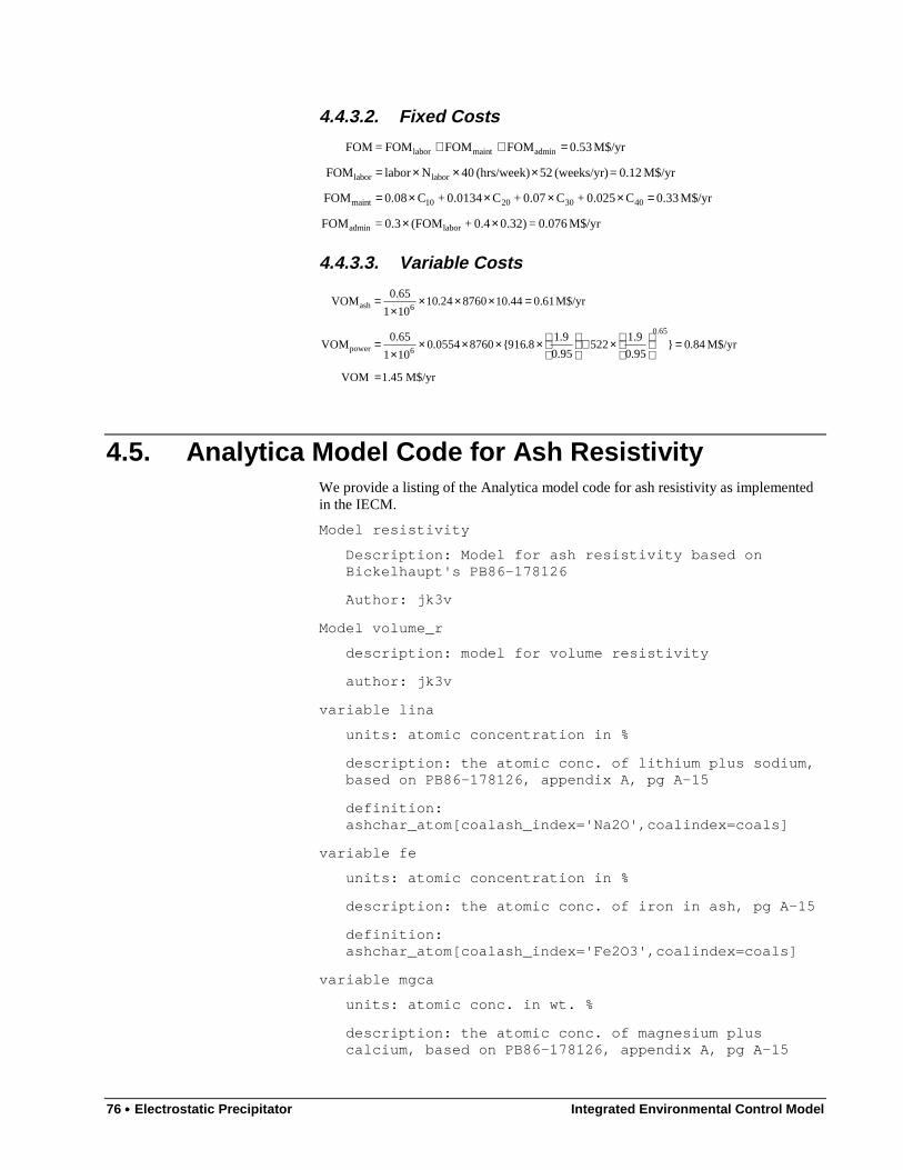
76 •••• Electrostatic Precipitator Integrated Environmental Control Model
4.4.3.2. Fixed Costs
M$/yr 0.076 = 0.32) 0.4 + (FOM0.3 =FOM
M$/yr 0.33 C0.025 + C0.07 + C0.0134 + C0.08 FOM
M$/yr 0.12 = (weeks/yr) 52 (hrs/week) 40 N labor FOM
M$/yr 0.53 FOMFOMFOM = FOM
laboradmin
40302010maint
laborlabor
adminmaintlabor
××
=××××=
×××=
=++
4.4.3.3. Variable Costs
M$/yr 45.1 VOM
M$/yr 84.0}95.0
9.1522
95.0
9.18.916{87600554.0
101
65.0VOM
M$/yr 61.044.10876024.10101
65.0 VOM
65.0
6power
6ash
=
=
×+
××××
×=
=××××
=
4.5. Analytica Model Code for Ash ResistivityWe provide a listing of the Analytica model code for ash resistivity as implementedin the IECM.
Model resistivity
Description: Model for ash resistivity based onBickelhaupt's PB86-178126
Author: jk3v
Model volume_r
description: model for volume resistivity
author: jk3v
variable lina
units: atomic concentration in %
description: the atomic conc. of lithium plus sodium,based on PB86-178126, appendix A, pg A-15
definition:ashchar_atom[coalash_index='Na2O',coalindex=coals]
variable fe
units: atomic concentration in %
description: the atomic conc. of iron in ash, pg A-15
definition:ashchar_atom[coalash_index='Fe2O3',coalindex=coals]
variable mgca
units: atomic conc. in wt. %
description: the atomic conc. of magnesium pluscalcium, based on PB86-178126, appendix A, pg A-15
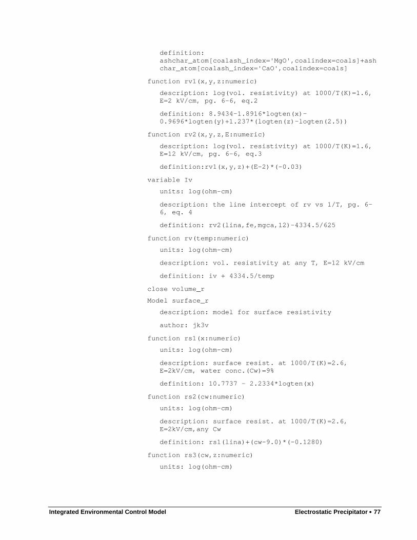
Integrated Environmental Control Model Electrostatic Precipitator •••• 77
definition:ashchar_atom[coalash_index='MgO',coalindex=coals]+ashchar_atom[coalash_index='CaO',coalindex=coals]
function rv1(x,y,z:numeric)
description: log(vol. resistivity) at 1000/T(K)=1.6,E=2 kV/cm, pg. 6-6, eq.2
definition: 8.9434-1.8916*logten(x)-0.9696*logten(y)+1.237*(logten(z)-logten(2.5))
function rv2(x,y,z,E:numeric)
description: log(vol. resistivity) at 1000/T(K)=1.6,E=12 kV/cm, pg. 6-6, eq.3
definition:rv1(x,y,z)+(E-2)*(-0.03)
variable Iv
units: log(ohm-cm)
description: the line intercept of rv vs 1/T, pg. 6-6, eq. 4
definition: rv2(lina,fe,mgca,12)-4334.5/625
function rv(temp:numeric)
units: log(ohm-cm)
description: vol. resistivity at any T, E=12 kV/cm
definition: iv + 4334.5/temp
close volume_r
Model surface_r
description: model for surface resistivity
author: jk3v
function rs1(x:numeric)
units: log(ohm-cm)
description: surface resist. at 1000/T(K)=2.6,E=2kV/cm, water conc.(Cw)=9%
definition: 10.7737 - 2.2334*logten(x)
function rs2(cw:numeric)
units: log(ohm-cm)
description: surface resist. at 1000/T(K)=2.6,E=2kV/cm,any Cw
definition: rs1(lina)+(cw-9.0)*(-0.1280)
function rs3(cw,z:numeric)
units: log(ohm-cm)
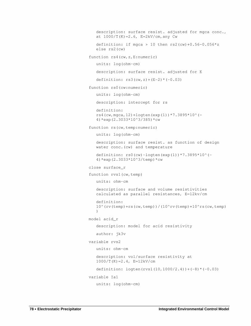
78 •••• Electrostatic Precipitator Integrated Environmental Control Model
description: surface resist. adjusted for mgca conc.,at 1000/T(K)=2.6, E=2kV/cm,any Cw
definition: if mgca > 10 then rs2(cw)+0.56-0.056*zelse rs2(cw)
function rs4(cw,z,E:numeric)
units: log(ohm-cm)
description: surface resist. adjusted for E
definition: rs3(cw,z)+(E-2)*(-0.03)
function rs0(cw:numeric)
units: log(ohm-cm)
description: intercept for rs
definition:rs4(cw,mgca,12)+logten(exp(1))*7.3895*10^(-4)*exp(2.3033*10^3/385)*cw
function rs(cw,temp:numeric)
units: log(ohm-cm)
description: surface resist. as function of designwater conc.(cw) and temperature
definition: rs0(cw)-logten(exp(1))*7.3895*10^(-4)*exp(2.3033*10^3/temp)*cw
close surface_r
function rvs1(cw,temp)
units: ohm-cm
description: surface and volume resistivitiescalculated as parallel resistances, E=12kv/cm
definition:10^(rv(temp)+rs(cw,temp))/(10^rv(temp)+10^rs(cw,temp))
model acid_r
description: model for acid resistivity
author: jk3v
variable rvs2
units: ohm-cm
description: vol/surface resistivity at1000/T(K)=2.4, E=12kV/cm
definition: logten(rvs1(10,1000/2.4))+(-8)*(-0.03)
variable Ia1
units: log(ohm-cm)

Integrated Environmental Control Model Electrostatic Precipitator •••• 79
description: intercept for ra1 based on mgca, feconc.
definition: if mgca < 5 and fe < 1 then 2.6354 else0.2915
variable ra1
units: log(ohm-cm)
description: acid resist. at 4ppm SO3, 10% H2O, 417K,4kV/cm
definition: ia1 + 0.7669*rvs2
variable sa
units:
description: coefficient for ra2
definition: if mgca < 5 and fe < 1 then -5.0 else -2.0502
variable ia2
units
description: intercept for ra2
definition: ra1 - sa*logten(4)
function ra2(ca:numeric)
units: log(ohm-cm)
description: acid resist. at 4kV/cm,10%H2O, 417K, andany ca
definition: ia2 + sa*logten(ca)
Index acid_i
description: index for sa1 based on so3 conc.
definition: ['1','2','3']
variable atom_i
description: index for sa1 based on lina, mgca, andfe conc.
definition: ['1','2','3']
variable acid_v
description: value of sa1 index based on so3 conc.
definition: if so3ppm(esp_gasin) < 2.75 then '1' elseif so3ppm(esp_gasin) > 6.5 then '3' else '2'
variable atom_v
description: value of sa1 based on mgca etc conc.
definition: if lina > 1 and mgca > 5 then '1' else iffe < 1 and mgca < 3 then '2' else '3'
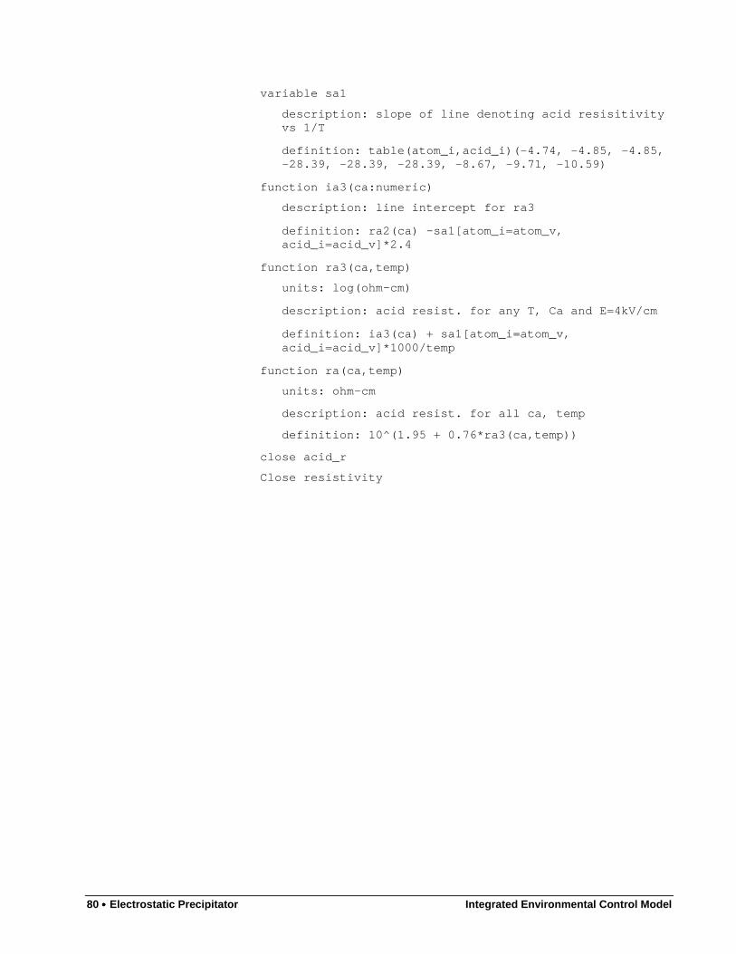
80 •••• Electrostatic Precipitator Integrated Environmental Control Model
variable sa1
description: slope of line denoting acid resisitivityvs 1/T
definition: table(atom_i,acid_i)(-4.74, -4.85, -4.85,-28.39, -28.39, -28.39, -8.67, -9.71, -10.59)
function ia3(ca:numeric)
description: line intercept for ra3
definition: ra2(ca) -sa1[atom_i=atom_v,acid_i=acid_v]*2.4
function ra3(ca,temp)
units: log(ohm-cm)
description: acid resist. for any T, Ca and E=4kV/cm
definition: ia3(ca) + sa1[atom_i=atom_v,acid_i=acid_v]*1000/temp
function ra(ca,temp)
units: ohm-cm
description: acid resist. for all ca, temp
definition: 10^(1.95 + 0.76*ra3(ca,temp))
close acid_r
Close resistivity
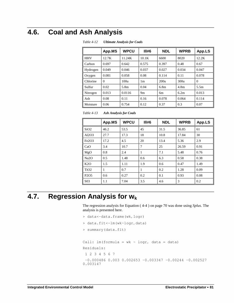
Integrated Environmental Control Model Electrostatic Precipitator •••• 81
4.6. Coal and Ash AnalysisTable 4-12 Ultimate Analysis for Coals
App.MS WPCU Ill#6 NDL WPRB App.LS
HHV 12.7K 11.24K 10.1K 6600 8020 12.2K
Carbon 0.697 0.642 0.575 0.397 0.48 0.67
Hydrogen 0.049 0.046 0.037 0.027 0.034 0.047
Oxygen 0.081 0.058 0.08 0.114 0.11 0.078
Chlorine 0 100u 1m 200u 300u 0
Sulfur 0.02 5.8m 0.04 6.8m 4.8m 5.5m
Nitrogen 0.013 0.0116 9m 6m 6.2m 0.013
Ash 0.08 0.11 0.16 0.078 0.064 0.114
Moisture 0.06 0.754 0.12 0.37 0.3 0.07
Table 4-13 Ash Analysis for Coals
App.MS WPCU Ill#6 NDL WPRB App.LS
SiO2 46.2 53.5 45 31.5 36.85 61
Al2O3 27.7 17.3 18 10.8 17.84 30
Fe2O3 17.2 4.5 20 13.4 5.36 2.9
CaO 3.4 10.7 7 25 26.59 0.91
MgO 0.8 2.4 1 7.1 5.48 0.76
Na2O 0.5 1.48 0.6 6.3 0.58 0.38
K2O 1.5 1.11 1.9 0.6 0.47 1.49
TiO2 1 0.7 1 0.2 1.28 0.09
P2O5 0.6 0.27 0.2 0.1 0.93 0.08
S03 1.1 7.04 3.5 4.6 3 0.2
4.7. Regression Analysis for w k
The regression analysis for Equation ( 4-4 ) on page 70 was done using Splus. Theanalysis is presented here.
> data<-data.frame(wk,logr)
> data.fit<-lm(wk~logr,data)
> summary(data.fit)
Call: lm(formula = wk ~ logr, data = data)
Residuals:
1 2 3 4 5 6 7
-0.000486 0.003 0.002653 -0.003347 -0.00244 -0.0025270.003147
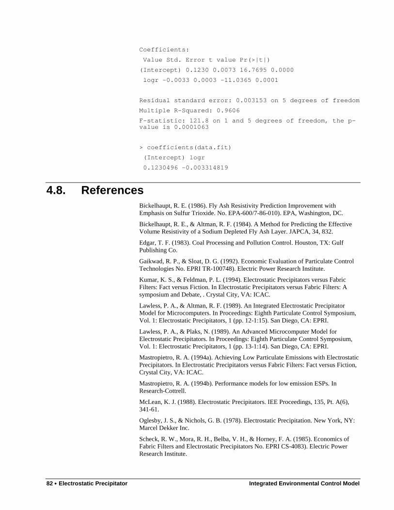
82 •••• Electrostatic Precipitator Integrated Environmental Control Model
Coefficients:
Value Std. Error t value Pr(>|t|)
(Intercept) 0.1230 0.0073 16.7695 0.0000
logr -0.0033 0.0003 -11.0365 0.0001
Residual standard error: 0.003153 on 5 degrees of freedom
Multiple R-Squared: 0.9606
F-statistic: 121.8 on 1 and 5 degrees of freedom, the p-value is 0.0001063
> coefficients(data.fit)
(Intercept) logr
0.1230496 -0.003314819
4.8. ReferencesBickelhaupt, R. E. (1986). Fly Ash Resistivity Prediction Improvement withEmphasis on Sulfur Trioxide. No. EPA-600/7-86-010). EPA, Washington, DC.
Bickelhaupt, R. E., & Altman, R. F. (1984). A Method for Predicting the EffectiveVolume Resistivity of a Sodium Depleted Fly Ash Layer. JAPCA, 34, 832.
Edgar, T. F. (1983). Coal Processing and Pollution Control. Houston, TX: GulfPublishing Co.
Gaikwad, R. P., & Sloat, D. G. (1992). Economic Evaluation of Particulate ControlTechnologies No. EPRI TR-100748). Electric Power Research Institute.
Kumar, K. S., & Feldman, P. L. (1994). Electrostatic Precipitators versus FabricFilters: Fact versus Fiction. In Electrostatic Precipitators versus Fabric Filters: Asymposium and Debate, . Crystal City, VA: ICAC.
Lawless, P. A., & Altman, R. F. (1989). An Integrated Electrostatic PrecipitatorModel for Microcomputers. In Proceedings: Eighth Particulate Control Symposium,Vol. 1: Electrostatic Precipitators, 1 (pp. 12-1:15). San Diego, CA: EPRI.
Lawless, P. A., & Plaks, N. (1989). An Advanced Microcomputer Model forElectrostatic Precipitators. In Proceedings: Eighth Particulate Control Symposium,Vol. 1: Electrostatic Precipitators, 1 (pp. 13-1:14). San Diego, CA: EPRI.
Mastropietro, R. A. (1994a). Achieving Low Particulate Emissions with ElectrostaticPrecipitators. In Electrostatic Precipitators versus Fabric Filters: Fact versus Fiction,Crystal City, VA: ICAC.
Mastropietro, R. A. (1994b). Performance models for low emission ESPs. InResearch-Cottrell.
McLean, K. J. (1988). Electrostatic Precipitators. IEE Proceedings, 135, Pt. A(6),341-61.
Oglesby, J. S., & Nichols, G. B. (1978). Electrostatic Precipitation. New York, NY:Marcel Dekker Inc.
Scheck, R. W., Mora, R. H., Belba, V. H., & Horney, F. A. (1985). Economics ofFabric Filters and Electrostatic Precipitators No. EPRI CS-4083). Electric PowerResearch Institute.

Integrated Environmental Control Model Electrostatic Precipitator •••• 83
Sloat, D. G. (1994). Coal Ash Resistivity. In Sargent & Lundy.
White, H. J. (1977). Electrostatic Precipitation of Fly Ash. JAPCA, 27(3), 206.
84 •••• Fabric Filter Integrated Environmental Control Model
5. Fabric Filter
5.1. IntroductionThis chapter describes the development of analytical models for the performance andcosts of high-performance particulate control technologies, focusing on fabric filters.Special attention is paid to developing models which can be used to estimate costsfor systems whose performance is up to a factor of three below the present NSPSstandards of 0.03 lb/MMBtu. Typically, the cost models relate the capital costs andthe operating and maintenance (O&M) costs to process parameters and the costs oflabor and materials. The capital cost models are anchored to a base capital cost for aspecific size unit and adjusted according to the actual or design parameters. Theperformance models are constructed to estimate the process parameters for a desiredlevel of emissions control. The primary motivation for these models is to estimatethe costs of complying with environmental standards on a basis which reflects recentadvances in control technology. Finally, we incorporate the uncertainties in variousprocess parameters and inputs costs so as to allow a more rational and robust basisfor comparing different technologies.
The initial development of the performance and cost models for fabric filters isdiscussed followed by a numerical example which illustrates the use of these newmodels. The next quarterly report will provide a similar update of the IECMelectrostatic precipitator models, plus a brief discussion of the comparativeadvantages of different particulate control.
5.2. Fabric Filters for Electric UtilitiesFabric filters have been very effective in achieving the 1979 NSPS limits for coal-fired power plants. As a result, over 100 baghouses associated with 20,000 MW ofgenerating capacity are in operation in the U.S. utility industry (Cushing, Bush, &Synder, 1990; Kumar & Feldman, 1994; Puille, 1985). These units routinely performat efficiencies above 99.9% and produce clear stack plumes with less than 1%opacity. These fabric filters have been in operation with pulverized coal-fired boilersof various designs including some which are installed on fluidized bed combustionboilers. Operating experience in the U.S. has been predominantly with reverse gascleaning (about 90%) with low air-to-cloth ratio baghouses. Bag failure rate hasstabilized at about 1% per year through the 1980s and four-year bag life is now fairlycommon. In particular, there has been virtually no reduction in boiler availability dueto baghouse malfunction since any target compartment can be brought off-line forbaghouse replacement.
Integrated Environmental Control Model Fabric Filter •••• 85
In this chapter, we will first discuss the important design parameters for fabric filtersand their effects on capital and O&M costs. The design parameters are dependent onthe bag cleaning method and this will be explicated. Cost models parameterized bydesign parameters are developed, along with a numerical example to illustrate thecost models.
5.3. Fabric Filter DesignFabric filters are essentially huge vacuum cleaners consisting of a large number oflong tubular filter bags arranged in parallel flow paths. As the ash-laden flue gaspasses through these filters, almost all of the particulate matter is removed. Ash thataccumulates on the bags is removed periodically by cleaning. For properly designedfabric filters, the size of the system is independent of the removal efficiency. Thus,efficiency can be improved without an associated increase in capital costs. The issueof a proper design is characterized by a number of parameters which we now discussin some detail. We also provide the default operating values used in the industrytoday with an estimate of uncertainty to bound the variation observed in practice(Belba, Grubb, & Chang, 1992; Carr & Smith, 1984; Cushing, et al., 1990; Scheck,Mora, Belba, & Horney, 1985; Sloat, Gaikwad, & Chang, 1993).
There are various bag cleaning techniques that are used and this influences otherprocess parameters in a non-trivial way. There are four available bag cleaningmethods:
1. Reverse Gas Cleaning (RG): This is an off-line bag cleaning techniquein which an auxiliary fan forces a relatively gentle flow of filtered fluegas backwards through the bags causing them to partially collapse anddislodge the dustcake. Over 90% of the U.S. utility baghouses usereverse-gas cleaning.
2. Reverse Gas/sonic cleaning (RG/S): A variation of RG in which lowfrequency pneumatic horns sound simultaneously with the flow ofreverse gas to add energy to the dustcake removal process.
3. Shake/Deflate Cleaning (S/D): A method for offline cleaning. The bagsare mechanically shaken immediately after or while a small quantity offiltered gas is forced back to relax the bags. The amount of filtered gasused is smaller than that used in RG cleaning.
4. Pulse-Jet Cleaning (PJ): A method for on-line cleaning in which pulsesof compressed air are blown down inside and through the bags toremove dustcake while the bags are filtering flue gas. Wire supportcages are used to prevent bag collapse during filtration and ash iscollected outside of the bags.
The choice of the bag cleaning method is usually based on the type of coal beingused (hence the filterability of the ash) and the historical experience with filtering theparticular kind of ash. The choice of the bag cleaning method is a design decisionand for the purposes of our models we assume that this is specified by the user.While reverse gas cleaning has been dominant in the past, studies have shown that itis not as effective as other methods in achieving low capital and O&M costs (Scheck,et al., 1985). RG/S and S/D impart more cleaning energy to the bags which results inthinner dustcakes and lower pressure drop. Such systems also can be at higher air-to-cloth (A/C) ratios, reducing costs. It appears that more recently, RG/S is emerging asa method of choice for full-scale, low A/C ratio utility baghouses on pulverized coal-fired boilers (Cushing, et al., 1990).

86 •••• Fabric Filter Integrated Environmental Control Model
The most critical parameter in the operation of a baghouse is the relative system sizewhich is characterized in terms of air-to-cloth ratio, defined as the volumetric flowrate of flue gas divided by the total bag cloth area. This ratio has the units ofacfm/ft2. The A/C ratio is determined based on the bag cleaning method, whichcontrols the residual quantity of the material remaining on the bags. This in turnaffects the resistance to gas flow and determines the pressure drop. Utility baghousestypically use A/C ratios of 1.5-4.0 acfm/ft2 (net-net)1 depending on the bag cleaningmethod. The cost of a baghouse is determined by the unit size which in turn dependson the gross A/C ratio and the volumetric flow rate. Given that the A/C ratio is theprimary determinant of the unit size, and hence the capital and operating costs, it isdesirable to operate at the highest A/C ratio that comfortably meets the performancespecifications. Table 5-1 provides the typical values used for A/C ratio for variousbaghouse types based on industry experience (Belba, et al., 1992; Bustard, Cushing,& Chang, 1992; Cushing, et al., 1990; Puille, 1985; Sloat, et al., 1993).
Baghouse pressure drop is caused by pressure losses in gas flow as it moves throughthe bag fabric and dustcake. The pressure drop is usually measured in inches of watergauge or column (iwg or iwc) and is a measure of the energy required to move fluegas through the baghouse structure and bags. Flange-to-flange pressure drop is thepressure difference measured between the baghouse inlet and outlet flanges. It is thesum of ductwork and tubesheet pressure drops. Tubesheet pressure drop is measuredacross the tubesheet in a single compartment and consists largely of the pressuredrop across the dustcake. Tubesheet pressure drop is the largest component of theflange-to-flange pressure drop and is useful since it can be controlled by theoperator. However, it is the flange-to-flange pressure drop that is used in terms of aunit's energy consumption during operation and is used for sizing the ID fan.Baghouses are generally designed for a flange-to-flange pressure drop of about 6 -8in. H2O regardless of the cleaning method as a result of constraints from induceddraft fans, ductwork stiffening, and other design details. Typical values for tubesheetpressure drop for given values of A/C ratios based on industry experience are alsoprovided in Table 5-1.
Table 5-1 Typical Fabric Filter Design Parameters
Baghouse Type A/C Ratio net-net(acfm/ft 2)
Averagetubesheet ∆∆∆∆P (in.
H2O)
Average BagLife (years)
Reverse Gas 1.7 -2.0 3 x (A/C) +/- 20% 3-5
Reverse Gas Sonic 1.7 -2.0 2.5 x (A/C) +/- 20% 3-5
Shake-Deflate 2.5 - 3.0 2 x (A/C) +/- 15% 2-4
Pulse Jet 4.0 - 4.5 1.3 x (A/C) +/- 50% 2-4
U.S. utilities largely use woven fiberglass bag fabric because of high flue gastemperatures. Fiberglass can withstand temperatures up to 500 F and can be texturedto control dustcake formation. But it is also susceptible to abrasion wear. The choiceof the bag fabric affects the cost of the bag. Bags generally fall into two sizecategories: 30-36 ft in length and 1 ft in diameter, and 20 -22 ft in length and 8 in. indiameter. Bag life is generally not an issue (except for manufacturing defects andimproper installation) and is usually between 3-5 years. All these parametersinfluence both the capital and operating costs. Once again, for the purposes of themodels developed here these parameters are treated as design variables to bespecified by the user. The effect of these choices on the cost of the baghouse hasbeen modeled.

Integrated Environmental Control Model Fabric Filter •••• 87
5.4. Cost Models for Fabric FiltersThe cost models for the four types of fabric filters are developed for both capitalcosts and operation and maintenance (O&M) costs. These models follow theeconomic premises for cost development and breakdown developed by EPRI. Thecapital costs are developed on a process area by process area basis and the O&M aredeveloped to reflect the fixed and the variable operating costs. The cost areas areshown in Table 5-2.
Table 5-2 Process Areas for Fabric Filter cost Models
Process Area Description
10 Collectors
20 Ductwork
30 Fly Ash Handling System
40 Differential Cost
The models developed in this report are based on price quotes from equipmentvendors obtained for EPRI (Gaikwad & Sloat, 1992; Scheck, et al., 1985). The maindifference in our treatment of these costs is that we have developed cost modelsparametrized by operating design parameters on a process area basis. In contrast, theEPRI models use aggregate costs (such as total capital requirement) for thedevelopment of parametrized models. In this subsection, we first present themethodological basis used for model development and then present the cost models.
In the development of cost models, we have treated the Reverse-Gas, ReverseGas/Sonic and the Shake-Deflate baghouses as one class of systems and the Pulse-Jetfabric filter separately as another class. Engineering experience suggests that thedifference in the economics between RG, RG/S, and SD baghouses can be treatedparametrically through the operating design parameters A/C, ∆P, and bag life(Scheck, et al., 1985). This implies that the difference in costs between a RGbaghouse and a RG/S baghouse is largely accounted by the difference in the designparameters and can be described by one set of cost models. The cost models forPulse-Jet baghouses have been developed separately since it is a new technology andthere is not sufficient experience to treat it parametrically in the context of the RGmodels.
The major design parameters which can significantly impact the total system cost ofthe fabric filter are gas flow volume (which depends on the generating unit size), A/Cratio, the flange-to-flange pressure drop in the baghouse, bag life and the bag fabricthat is used for filtering. The costs of baghouses for different unit sizes and withvariations in the above parameters are reflected in the models. The sensitivity ofbaghouse costs to variations in these parameters is analyzed to parameterize the costmodels. We will now discuss in detail the experimental design and development thecost models for each system of baghouses separately.
5.4.1. Reverse Gas SystemsThe experimental design used to choose different vectors of the design parametersfor capital cost estimation (Scheck, et al., 1985) is shown in Table 5-3.

88 •••• Fabric Filter Integrated Environmental Control Model
Table 5-3 Range of Model Design Parameters
Case Size in MW(acfm)
A/C Ratio(gross) cfm/ft 2
Bags per Compartment(No. of Compartments)
Base 500 MW (1.9 M) 2.0 360 (28)
1 250 MW (0.95 M) 2.0 360 (14)
2 1000 MW (3.8 M) 2.0 360 (56)
3 500 MW (1.9M) 1.6 396 (32)
4 500 MW (1.9M) 3.6 396 (14)
5 500 MW (1.9M) 2.0 648 (16)
6 500 MW (1.9M) 2.0 252 (40)
Range 250-1000 MW 1.6-3.6 252-648
The costs for each vector of parameters in Table 5-3, broken down by process area isprovided in Table 5-4 based on a 1984 EPRI study (Scheck, et al. 1984). These costsare used only to obtain an exponential scaling factor for each process area. Theactual cost-models are based on 1990 dollars.
Table 5-4 Process Area Capital Costs Used for Scaling Parameter Estimation (1982$/kW)
ProcessArea
Case 1 Case 2 Case 3 Case 4 Case 5 Case 6 BaseCase
10 39.51 32.51 43.23 22.16 32.87 37.84 35.86
20 0.85 0.60 0.71 0.72 0.71 0.71 0.71
30 8.90 4.75 6.45 5.24 5.26 6.73 6.01
40 1.85 1.85 1.50 4.02 4.02 1.85 1.85
Total 51.11 39.71 51.89 32.14 40.69 47.13 44.43
The mathematical model to describe the sensitivity of cost models to parametervariations is normalized against the cost for the base case. The general form of thecost model for each process area is as shown below:
cbaf
i
i
SIL
SIL
B
B
CA
CA
G
G
PC
PC
×
×
×
=
/
//
// /
/ ( 5-1 )
where
PCi = process area capital, 1990 $
PCi/ = process area capital, base case, 1990 $
G = inlet gas flow, acfm
G/ = inlet gas flow, base case, acfm
A/C = air-to-cloth ratio, acfm/ft2
A/C/ = air-to-cloth ratio, base case, acfm/ft2
B = bags per compartment
B/ = bags per compartment, base case
SIL = ash rate to silo, tons/hr
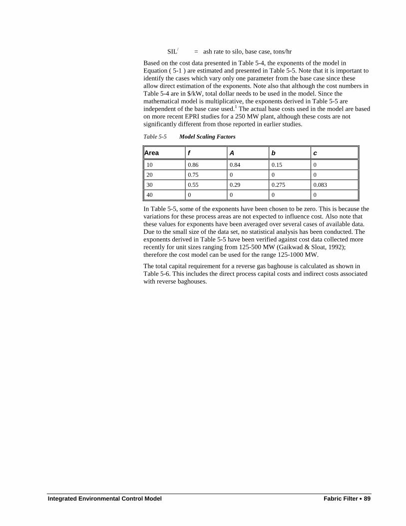
Integrated Environmental Control Model Fabric Filter •••• 89
SIL/ = ash rate to silo, base case, tons/hr
Based on the cost data presented in Table 5-4, the exponents of the model inEquation ( 5-1 ) are estimated and presented in Table 5-5. Note that it is important toidentify the cases which vary only one parameter from the base case since theseallow direct estimation of the exponents. Note also that although the cost numbers inTable 5-4 are in $/kW, total dollar needs to be used in the model. Since themathematical model is multiplicative, the exponents derived in Table 5-5 areindependent of the base case used.1 The actual base costs used in the model are basedon more recent EPRI studies for a 250 MW plant, although these costs are notsignificantly different from those reported in earlier studies.
Table 5-5 Model Scaling Factors
Area f A b c
10 0.86 0.84 0.15 0
20 0.75 0 0 0
30 0.55 0.29 0.275 0.083
40 0 0 0 0
In Table 5-5, some of the exponents have been chosen to be zero. This is because thevariations for these process areas are not expected to influence cost. Also note thatthese values for exponents have been averaged over several cases of available data.Due to the small size of the data set, no statistical analysis has been conducted. Theexponents derived in Table 5-5 have been verified against cost data collected morerecently for unit sizes ranging from 125-500 MW (Gaikwad & Sloat, 1992);therefore the cost model can be used for the range 125-1000 MW.
The total capital requirement for a reverse gas baghouse is calculated as shown inTable 5-6. This includes the direct process capital costs and indirect costs associatedwith reverse baghouses.
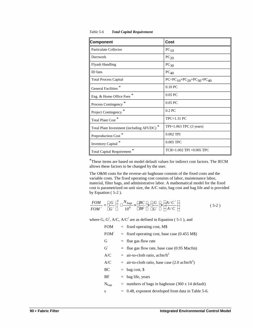
90 •••• Fabric Filter Integrated Environmental Control Model
Table 5-6 Total Capital Requirement
Component Cost
Particulate Collector PC10
Ductwork PC20
Flyash Handling PC30
ID fans PC40
Total Process Capital PC=PC10+PC20+PC30+PC40
General Facilities * 0.10 PC
Eng. & Home Office Fees * 0.05 PC
Process Contingency * 0.05 PC
Project Contingency * 0.2 PC
Total Plant Cost * TPC=1.31 PC
Total Plant Investment (including AFUDC) * TPI=1.063 TPC (3 years)
Preproduction Cost * 0.002 TPI
Inventory Capital * 0.005 TPC
Total Capital Requirement * TCR=1.002 TPI +0.005 TPC
*These items are based on model default values for indirect cost factors. The IECMallows these factors to be changed by the user.
The O&M costs for the reverse-air baghouse consists of the fixed costs and thevariable costs. The fixed operating cost consists of labor, maintenance labor,material, filter bags, and administrative labor. A mathematical model for the fixedcost is parametrized on unit size, the A/C ratio, bag cost and bag life and is providedby Equation ( 5-2 ).
×
×
×+
=
CA
CA
G
G
BF
BCN
G
G
FOM
FOM bagss
/
/
10
/
/6// ( 5-2 )
where G, G/, A/C, A/C/ are as defined in Equation ( 5-1 ), and
FOM = fixed operating cost, M$
FOM/ = fixed operating cost, base case (0.455 M$)
G = flue gas flow rate
G/ = flue gas flow rate, base case (0.95 Macfm)
A/C = air-to-cloth ratio, acfm/ft2
A/C = air-to-cloth ratio, base case (2.0 acfm/ft2)
BC = bag cost, $
BF = bag life, years
Nbags = numbers of bags in baghouse (360 x 14 default)
s = 0.48, exponent developed from data in Table 5-6.
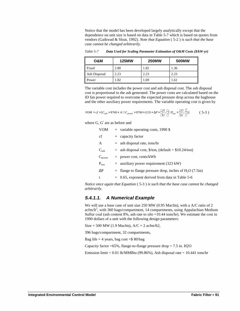
Integrated Environmental Control Model Fabric Filter •••• 91
Notice that the model has been developed largely analytically except that thedependence on unit size is based on data in Table 5-7 which is based on quotes fromvendors (Gaikwad & Sloat, 1992). Note that Equation ( 5-2 ) is such that the basecase cannot be changed arbitrarily.
Table 5-7 Data Used for Scaling Parameter Estimation of O&M Costs ($/kW-yr)
O&M 125MW 250MW 500MW
Fixed 2.80 1.82 1.36
Ash Disposal 2.23 2.23 2.23
Power 1.82 1.69 1.61
The variable cost includes the power cost and ash disposal cost. The ash disposalcost is proportional to the ash generated. The power costs are calculated based on theID fan power required to overcome the expected pressure drop across the baghouseand the other auxiliary power requirements. The variable operating cost is given by
)]135(87608760[//
t
auxpowerashG
GP
G
GPCACcfVOM
×+
×∆×××+×××= ( 5-3 )
where G, G/ are as before and
VOM = variable operating costs, 1990 $
cf = capacity factor
A = ash disposal rate, tons/hr
Cash = ash disposal cost, $/ton, (default = $10.24/ton)
Cpower = power cost, cents/kWh
Paux = auxiliary power requirement (323 kW)
∆P = flange to flange pressure drop, inches of H2O (7.5in)
t = 0.65, exponent derived from data in Table 5-6
Notice once again that Equation ( 5-3 ) is such that the base case cannot be changedarbitrarily.
5.4.1.1. A Numerical ExampleWe will use a base case of unit size 250 MW (0.95 Macfm), with a A/C ratio of 2acfm/ft2, with 360 bags/compartment, 14 compartments, using Appalachian MediumSulfur coal (ash content 8%, ash rate to silo =10.44 tons/hr). We estimate the cost in1990 dollars of a unit with the following design parameters:
Size = 500 MW (1.9 Macfm), A/C = 2 acfm/ft2,
396 bags/compartment, 32 compartments,
Bag life = 4 years, bag cost =$ 80/bag
Capacity factor =65%, flange-to-flange pressure drop = 7.5 in. H2O
Emission limit = 0.01 lb/MMBtu (99.86%), Ash disposal rate = 10.441 tons/hr
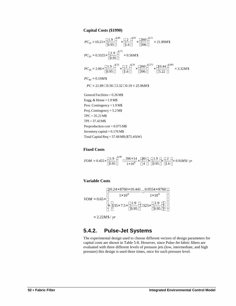
92 •••• Fabric Filter Integrated Environmental Control Model
Capital Costs ($1990)
$96.2519.032.356.089.21
$19.0
$32.322.5
44.10
396
360
6.1
2
95.0
9.106.2
$56.095.0
9.13325.0
$89.21396
360
6.1
2
95.0
9.121.10
40
083.0275.029.055.0
30
75.0
20
15.081.086.0
10
MPC
MPC
MPC
MPC
MPC
=+++=
=
=
×
×
×
×=
=
×=
=
×
×
×=
($75.4/kW) M$ 37.68 = Req Capital Total
M$ 0.176 = capitalInventory
M$ 0.075 =cost ion Preproduct
M$ 37.43 = TPI
M$ 35.21 = TPC
M$ 5.2 =y Contingenc Proj.
M$ 1.9 =y Contingenc Proc.
M$ 1.9 = Home & Engg.
M$ 0.26 = Facilities General
Fixed Costs
yrMFOM /$91.06.1
2
95.0
9.1
4
80
101
14396
95.0
9.1455.0
6
48.0
=
×
×
×
××+
×=
Variable Costs
yrM
VOM
/$22.2
95.0
9.1323
95.0
9.15.7135
101
87600554.0
101
441.10876024.10
65.0
66
=
×+
×××
××+
×××
×=
5.4.2. Pulse-Jet SystemsThe experimental design used to choose different vectors of design parameters forcapital costs are shown in Table 5-8. However, since Pulse-Jet fabric filters areevaluated with three different levels of pressure jets (low, intermediate, and highpressure) this design is used three times, once for each pressure level.
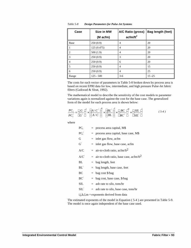
Integrated Environmental Control Model Fabric Filter •••• 93
Table 5-8 Design Parameters for Pulse-Jet Systems
Case Size in MW
(M acfm)
A/C Ratio (gross)
acfm/ft 2
Bag length (feet)
Base 250 (0.9) 4 20
1 125 (0.475) 4 20
2 500 (1.9) 4 20
3 250 (0.9) 3 20
4 250 (0.9) 6 20
5 250 (0.9) 4 15
6 250 (0.9) 4 25
Range 125 - 500 3-6 15 -25
The costs for each vector of parameters in Table 5-8 broken down by process area isbased on recent EPRI data for low, intermediate, and high pressure Pulse-Jet fabricfilters (Gaikwad & Sloat, 1992).
The mathematical model to describe the sensitivity of the cost models to parametervariations again is normalized against the cost for the base case. The generalizedform of the model for each process area is shown below:
imlkj
i
i
SIL
SIL
BC
BC
BL
BL
CA
CA
G
G
PC
PC
×
×
×
×
=
//
//
// /
/ ( 5-4 )
where
PCi = process area capital, M$
PCi/ = process area capital, base case, M$
G = inlet gas flow, acfm
G/ = inlet gas flow, base case, acfm
A/C = air-to-cloth ratio, acfm/ft2
A/C/ = air-to-cloth ratio, base case, acfm/ft2
BL = bag length, feet
BL/ = bag length, base case, feet
BC = bag cost $/bag
BC/ = bag cost, base case, $/bag
SIL = ash rate to silo, tons/hr
SIL/ = ash rate to silo, base case, tons/hr
i,j,k,l,m = exponents derived from data
The estimated exponents of the model in Equation ( 5-4 ) are presented in Table 5-9.The model is once again independent of the base case used.
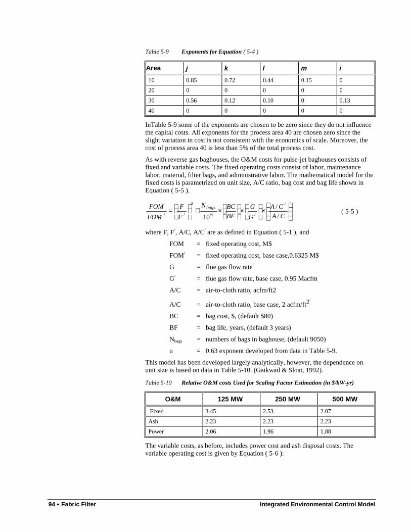
94 •••• Fabric Filter Integrated Environmental Control Model
Table 5-9 Exponents for Equation ( 5-4 )
Area j k l m i
10 0.85 0.72 0.44 0.15 0
20 0 0 0 0 0
30 0.56 0.12 0.10 0 0.13
40 0 0 0 0 0
InTable 5-9 some of the exponents are chosen to be zero since they do not influencethe capital costs. All exponents for the process area 40 are chosen zero since theslight variation in cost is not consistent with the economics of scale. Moreover, thecost of process area 40 is less than 5% of the total process cost.
As with reverse gas baghouses, the O&M costs for pulse-jet baghouses consists offixed and variable costs. The fixed operating costs consist of labor, maintenancelabor, material, filter bags, and administrative labor. The mathematical model for thefixed costs is parametrized on unit size, A/C ratio, bag cost and bag life shown inEquation ( 5-5 ).
×
×
×+
=
CA
CA
G
G
BF
BCN
F
F
FOM
FOM bagsu
/
/
10
/
/6// ( 5-5 )
where F, F/, A/C, A/C/ are as defined in Equation ( 5-1 ), and
FOM = fixed operating cost, M$
FOM/ = fixed operating cost, base case,0.6325 M$
G = flue gas flow rate
G/ = flue gas flow rate, base case, 0.95 Macfm
A/C = air-to-cloth ratio, acfm/ft2
A/C = air-to-cloth ratio, base case, 2 acfm/ft2
BC = bag cost, $, (default $80)
BF = bag life, years, (default 3 years)
Nbags = numbers of bags in baghouse, (default 9050)
u = 0.63 exponent developed from data in Table 5-9.
This model has been developed largely analytically, however, the dependence onunit size is based on data in Table 5-10. (Gaikwad & Sloat, 1992).
Table 5-10 Relative O&M costs Used for Scaling Factor Estimation (in $/kW-yr)
O&M 125 MW 250 MW 500 MW
Fixed 3.45 2.53 2.07
Ash 2.23 2.23 2.23
Power 2.06 1.96 1.88
The variable costs, as before, includes power cost and ash disposal costs. Thevariable operating cost is given by Equation ( 5-6 ):
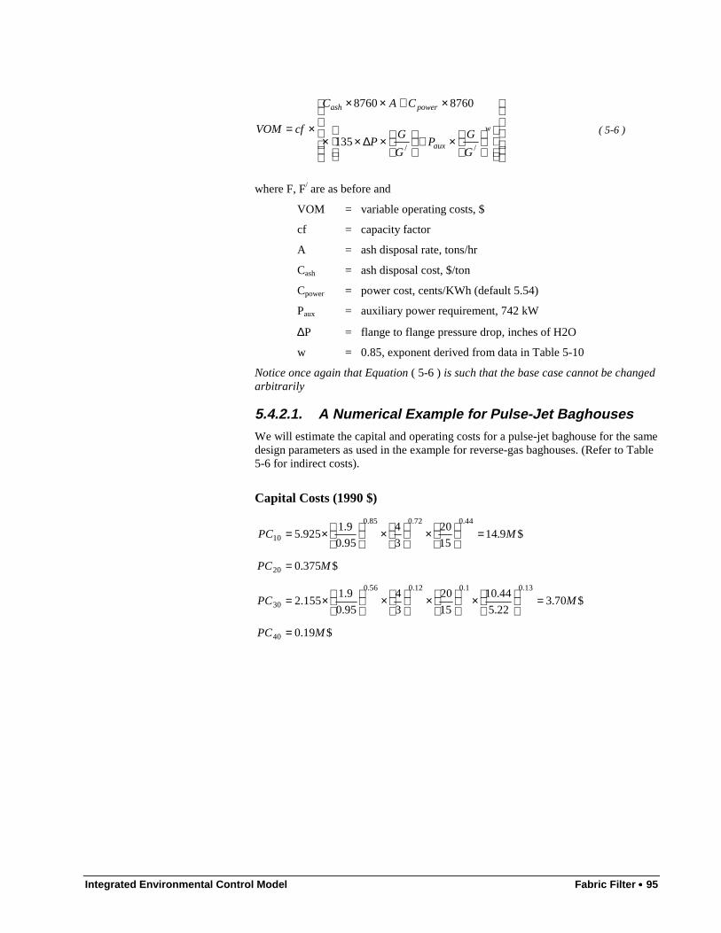
Integrated Environmental Control Model Fabric Filter •••• 95
×+
×∆××
×+××
×= w
aux
powerash
G
GP
G
GP
CAC
cfVOM
//135
87608760
( 5-6 )
where F, F/ are as before and
VOM = variable operating costs, $
cf = capacity factor
A = ash disposal rate, tons/hr
Cash = ash disposal cost, $/ton
Cpower = power cost, cents/KWh (default 5.54)
Paux = auxiliary power requirement, 742 kW
∆P = flange to flange pressure drop, inches of H2O
w = 0.85, exponent derived from data in Table 5-10
Notice once again that Equation ( 5-6 ) is such that the base case cannot be changedarbitrarily
5.4.2.1. A Numerical Example for Pulse-Jet BaghousesWe will estimate the capital and operating costs for a pulse-jet baghouse for the samedesign parameters as used in the example for reverse-gas baghouses. (Refer to Table5-6 for indirect costs).
Capital Costs (1990 $)
$19.0
$70.322.5
44.10
15
20
3
4
95.0
9.1155.2
$375.0
$9.1415
20
3
4
95.0
9.1925.5
40
13.01.012.056.0
30
20
44.072.085.0
10
MPC
MPC
MPC
MPC
=
=
×
×
×
×=
=
=
×
×
×=
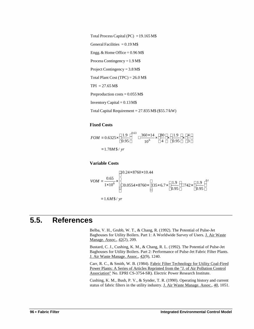
96 •••• Fabric Filter Integrated Environmental Control Model
($55.7/kW) M$ 27.835 =t Requiremen Capital Total
M$ 0.13 = CapitalInventory
M$ 0.055 = costsion Preproduct
M$ 27.65 = TPI
M$ 26.0 = (TPC)Cost Plant Total
M$ 3.8 =y ContingencProject
M$ 1.9 =y Contingenc Process
M$ 0.96 = Office Home&Engg.
M$ 0.19 = Facilities General
M$ 19.165 = (PC) Capital Process Total
Fixed Costs
yrM
FOM
/$78.1
3
4
95.0
9.1
4
80
10
14360
95.0
9.16325.0
6
63.0
=
×
×
××+
×=
Variable Costs
yrM
VOM
/$6.1
95.0
9.1742
95.0
9.17.613587600554.0
44.10876024.10
101
65.08.0
6
=
×+
××××+
××
××
=
5.5. ReferencesBelba, V. H., Grubb, W. T., & Chang, R. (1992). The Potential of Pulse-JetBaghouses for Utility Boilers. Part 1: A Worldwide Survey of Users. J. Air WasteManage. Assoc., 42(2), 209.
Bustard, C. J., Cushing, K. M., & Chang, R. L. (1992). The Potential of Pulse-JetBaghouses for Utility Boilers. Part 2: Performance of Pulse-Jet Fabric Filter Plants.J. Air Waste Manage. Assoc., 42(9), 1240.
Carr, R. C., & Smith, W. B. (1984). Fabric Filter Technology for Utility Coal-FiredPower Plants: A Series of Articles Reprinted from the "J. of Air Pollution ControlAssociation" No. EPRI CS-3754-SR). Electric Power Research Institute.
Cushing, K. M., Bush, P. V., & Synder, T. R. (1990). Operating history and currentstatus of fabric filters in the utility industry. J. Air Waste Manage. Assoc., 40, 1051.
Integrated Environmental Control Model Fabric Filter •••• 97
Gaikwad, R. P., & Sloat, D. G. (1992). Economic Evaluation of Particulate ControlTechnologies No. EPRI TR-100748). Electric Power Research Institute.
Kumar, K. S., & Feldman, P. L. (1994). Electrostatic Precipitators versus FabricFilters: Fact versus Fiction. In Electrostatic Precipitators versus Fabric Filters: ASymposium and Debate, . Crystal City, VA: ICAC.
Puille, W. (1985). 1985 Update, Operating History and Current Status in the UtilityIndustry. In Third Conference on Fabric Filter Technology for Coal Fired PowerPlants, . Scottsdale, AZ:
Scheck, R. W., Mora, R. H., Belba, V. H., & Horney, F. A. (1985). Economics ofFabric Filters and Electrostatic Precipitators No. EPRI CS-4083). Electric PowerResearch Institute.
Sloat, D. G., Gaikwad, R. P., & Chang, R. L. (1993). The Potential of Pulse-JetBaghouses for Utility Boilers. Part 3: Comparative Economics of Pulse-JetBaghouse, Precipitators and Reverse-Gas Baghouses. J. Air Waste Manage. Assoc.,43, 120.
98 •••• Flue Gas Desulfurization Integrated Environmental Control Model
6. Flue Gas Desulfurization
6.1. Background to FGD ModelsIn this chapter we describe the use of systematic sensitivity analysis and multivariateregression for the development of analytical models for the performance and cost ofhigh-performance wet lime/limestone FGD systems and dry lime sprayer systems.Special attention has been paid to FGD systems whose performance with respect tosulfur removal efficiency lies in the 90-98% range. The cost of using additives suchas dibasic acid (DBA) as a design option for achieving high performance is alsoexamined. The cost models developed relates the capital costs and the operating andmaintenance costs to input variables describing performance parameters and thecosts of labor and materials. Systematic sensitivity analysis is used to select and rankthe set of input variables and multivariate regression is used for the development offunctional relations between the input variables and costs (outputs). This systematicapproach along with engineering judgment is used to develop aggregate models forcosting high performance FGD systems. These aggregate models are appropriate insize and form for conducting uncertainty analysis using Monte Carlo methods in theIECM.
The chapter is organized as follows. Section 6.2 below describes the development ofnew FGD performance models. Based on a review of the literature, someapproximate functional relations to describe FGD performance are presented.Section 6.3 on page 108 provides an overview of the methodological approach usedto derive capital cost models. Four FGD systems are analyzed: (1) wet limestonewith forced oxidation (LSFO), (2) dibasic acid enhanced wet limestone (LS/DBA),(3) a magnesium-enhanced wet lime system, and (4) a spray dryer with lime. Therelations for direct process capital cost models are derived for each process area inSection 6.4 on page 116. The effects of different sparing philosophies on the capitalcost are also examined. Cost models are then developed for the fixed operating andmaintenance costs associated with operating a FGD system in Section 6.5 on page124. Section 6.6 on page 125 develops models for the variable costs of reagent use,power use, waste disposal, energy consumption etc. Section 6.7 on page 129provides a numerical example to illustrate the new models.
6.2. FGD Performance ModelsIn this section we describe the performance models used to provide key parameterinputs to the cost models described later. We begin with a brief survey of FGD
Integrated Environmental Control Model Flue Gas Desulfurization •••• 99
performance literature. Based on the literature, approximate functional relationsbetween performance parameters are developed.
The analysis in this chapter is geared towards developing updated performance andcost models for four commercial FGD processes:
1. Limestone with Forced Oxidation (LSFO): A limestone slurry is usedin an open spray tower with in-situ oxidation to remove SO2 and form agypsum sludge. The main advantages as compared to conventionalsystems is easier dewatering, more economical disposal of scrubberproducts, and decreased scaling on tower walls.
2. Limestone with Dibasic Acid Additive (LS/DBA): A modification toLSFO where dibasic acid (DBA) is added to act as a buffer/catalyst inthe open spray tower. The main advantages are increased SO2 removaland decreased liquid to gas ratio.
3. Magnesium Enhanced Lime System: A magnesium sulfite and limeslurry (maglime) is used to remove SO2 and form a precipitate high incalcium sulfite. The high alkalinity of the maglime slurry allows veryhigh SO2 removal. However, the reagent cost is also higher and solidwaste is not easily disposed.
4. Lime Spray Dryer: An atomized spray of a mixture of lime slurry andrecycled solids is brought into contact with the hot flue gas. The waterin the slurry evaporates leaving dry reaction products and flyash whichdrops out of the scrubber. A particulate control device such as abaghouse is also used to remove the rest of the dry products from theflue gas before releasing it. The SO2 removal efficiency is the total ofSO2 removed in the scrubber and the baghouse.
6.2.1. Wet Limestone FGD SystemsAdvanced wet limestone FGD systems are now designed to achieve SO2 removalefficiencies in excess of 95%. The single loop countercurrent spray tower is the mostcommonly used device for the removal of SO2. The design of spray towers for highefficiency without additives is achieved by using high liquid-to-gas (L/G) ratios andimproving gas/liquid contact by spray nozzle design (Bhat, et al., 1993; Rader &Bakke, 1991) On the other hand, organic acids such as dibasic acid or adipic acid areadded as buffers to improve performance (Blythe, et al., 1993; Moser & Owens,1990; Smolenski, et al., 1993; Stevens, et al., 1993) In this section, brief descriptionsand approximate relations for high performance LSFO and LS/DBA systems areprovided. The approximate relations are gleaned from the literature to reflect USexperience with high performance wet limestone FGD systems (Benson, 1993; Dene,et al., 1991; Johnson, 1993; Klingspor, 1993; Laslow, 1993; Moser & Owens, 1990;Noblett Jr., et al., 1990; Noblett Jr., 1993; Rader, 1993; Rader & Bakke, 1991;Smolenski, et al., 1993; Stevens, et al., 1993; Stevens, et al., 1991; Weilert, 1993;Weilert & Ratliff, 1990). The paragraph below provides some background (Corbett,et al., 1977; Noblett Jr., et al., 1990) for the scrubbing process, which is useful inunderstanding the bases for the relations, provided later.
The removal of SO2 from flue gas in a lime/limestone scrubber depends on a gas-liquid-solid mass transfer process. The sulfur dioxide is transferred from the flue gasto the slurry liquid in the scrubber and subsequently precipitated as calcium salts. Inthis section we provide a very brief discussion of the key factors that affect the SO2
removal efficiency from a theoretical standpoint. Against this backdrop we examineempirical data, which reflects the recent experience with high efficiency scrubbers,and develop an approximate response surface parameterized on the key variables.
100 •••• Flue Gas Desulfurization Integrated Environmental Control Model
The basis for the analysis of vapor-liquid mass transfer phenomena is the two-filmtheory in which the total resistance to mass transfer is expressed as the sum ofindividual resistances in the vapor and liquid phases near the interface. Based onexpressions for molar flux in the gas and liquid films and assuming that the liquid-vapor interface is at equilibrium (Corbett, et al., 1977; Mehta & Rochelle, 1983;Rochelle, 1981; Rochelle, 1981), the overall mass transfer coefficient is written as:
11
−
×+=
lgg ke
H
kK ( 6-1 )
where kg (mole/cm2-sec-atm) and kl (cm/sec) are individual gas and liquid phasemass transfer coefficients, H is a physical constant (atm/mol-liter) from Henry's Lawand e is an enhancement factor to account for chemical reactions that permit SO2 todiffuse through the liquid film as sulfite or bisulfite ions rather than as undissociatedSO2 (Chang and Rochelle 1980). The amount of SO2 transferred from gas phase perunit time is the integral of the molar flux and the interfacial area for mass transfer.This leads to an expression for SO2 removal efficiency as shown in Equation ( 6-2 ):
×××−−=
G
VPaK gSO exp1
2η ( 6-2 )
where
a = interfacial mass transfer area per unit volume
V = scrubber volume
P = total pressure in scrubber
G = molar gas flow rate
Kg = mass transfer coefficient
The interfacial area is determined by the contractor design, gas distribution in thescrubber and the gas and liquid flow rates (or residence time in the scrubber). V/G isthe residence time of flue gas in the scrubber and it depends on superficial velocityand size of the scrubber. The mass transfer coefficient, Kg is influenced by processvariables. Any process variable which affects the physical or chemical properties ofthe two films may affect Kg. The individual mass transfer coefficients kg and kl
describe the diffusion rates across two hypothetically stagnant films. In the followingparagraphs we discuss the effect of various process parameters on the SO2 removalefficiency and develop a response surface using the exponential form. All therelations developed in this section are based on a log-linear approximation, assuggested by Equation ( 6-1 ), and are developed as follows:
∑ ×+=
−−=
iii
SO
xbaRTU
RTU )1ln( 2η
( 6-3 )
where a and bi parameters which represent the linear slope of the effect of processparameters xi.
L/G is a key variable since it affects SO2 removal by increasing the available liquidphase alkalinity and the interfacial mass transfer area. Increasing the L/G ratio bringsmore alkaline materials into the scrubber per mole of SO2 scrubbed thus decreasingthe liquid film mass transfer resistance and improving the SO2 removal. This effect ismagnified by an associated increase in the interfacial mass transfer area which

Integrated Environmental Control Model Flue Gas Desulfurization •••• 101
improves efficiency. Industry practice is based on a log-linear relation between ηSO2
and L/G ratio (Benson, 1993; Bhat, et al., 1993; Dene, et al., 1991; Klingspor, 1993;Rader, 1993). Typical values for ηSO2
and L/G are provided in the table below.
Table 6-1 Typical Values for SO2 Removal and L/G.
ηSO2L/G(gpm/Kacfm)
90% 90
95% 130
Based on the values in the table above, an approximate relation2 between sulfurremoval efficiency and L/G is:
{ })/0175.0725.0(exp12
GLSO ×+−−=η ( 6-4 )
where L/G is measured in gpm/1000 acfm. The effect of lime/limestone scrubbingchemistry on SO2 removal can be understood by considering the mass transferresistance from the gas and liquid film separately.
6.2.1.1. Liquid Film Limited Mass TransferLimestone systems are generally at least partially liquid film mass transfer limited.The liquid film mass transfer resistance is a strong function of liquid phasealkalinity. When SO2 is absorbed by an aqueous scrubbing liquor, sulfurous acid isformed. Increasing the liquid phase or solid phase concentrations of alkalinematerials (such as CaCO3, CaSO3, Mg++) increases the liquid phase alkalinity whichin turn improves SO2 removal efficiency. Increasing the liquid phase alkalinitydecreases the Henry's Law constant which in turn decreases the mass transferresistance H/(e kl). The enhancement factor depends on the inlet SO2 concentrationand it decreases with increasing SO2 concentrations thus increasing the mass transferresistance. The kl portion of the mass transfer resistance is a function of thehydraulics of the scrubber and depends on gas distribution and the geometry ofscrubber.
Increasing the limestone stoichiometry (φ) improves liquid phase alkalinity and SO2
removal. However the effect saturates and little improvement in SO2 removal isobserved over 1.1. Limestone utilization varies inversely with the pH and is a criticalfactor for the operating costs of SO2 scrubbing. Most modern scrubbers are designedfor high utilization of about 95% or higher. Therefore stoichiometry affects theperformance in opposite ways. A detailed quantification of the effect ofstoichiometry on pH is not straightforward and needs the development of processsimulators (Agrawal & Rochelle, 1993; Noblett Jr., et al., 1990). It is possible to getan approximate idea of how SO2 removal is affected by pH and in turn by φ based onempirical data (Klingspor, 1993; Noblett Jr., et al., 1990; Rader, 1993; Stevens, etal., 1991) as shown in Table 6-2 below:
2 All relations developed in this section are based on a wet limestone/lime FGD tower with four spray headers per tower.The default process parameters are as follows: pH=5.3, φ=1.03, L/G=90, inlet SO2=1750 ppm (2.6% S coal), Cl =25,000ppm (in the slurry) and superficial velocity in tower=10 fps.
102 •••• Flue Gas Desulfurization Integrated Environmental Control Model
Table 6-2 Stoichiometry and Alkalinity Approximations
ηSO2 pH φφφφ
90% 5.3 1.03
95% 6.0 1.1
Based on these numbers a linear approximation for the effect of stoichiometry can berepresented by an additional term in Equation ( 6-4 ) as follows:
{ })]3.100.10(/0175.0725.0[exp12 −×+×+−−= φη GLSO ( 6-5 )
Notice that the effect of stoichiometry is represented as an increase in SO2 removaldue to an increase in pH (caused by increasing φ) over the default value of 5.3.
An increase in the inlet SO2 concentrations beyond 1000 ppm decreases theenhancement factor e which in turn increases the mass transfer resistance. Theenhancement factor is a function of gas and solution composition (Chang &Rochelle, 1983) which affects the conversion of SO2 to bisulfite. Typical values ofSO2 removal for different inlet SO2 concentrations are provided below based onindustry experience (Moser & Owens, 1990; Noblett Jr., et al., 1990; Stevens, et al.,1991).
Table 6-3 Inlet SO2 Concentration
ηSO2SO2 ppm
90% 2000 (2.8% S)
84% 4000 (4% S)
This can be represented by an additional term in Equation ( 6-5 ) which accounts forthe loss of removal efficiency as the inlet SO2 concentration increases over 2000ppm.
−×−
−×+×+−−=
− )]2000(105.2
)3.100.10(/0175.0725.0[exp1
24
2SO
GLSO
φη ( 6-6 )
Similarly calcium chloride accumulation in the slurry leads to a decrease in SO2
removal. Chloride accumulation suppresses the desirable effects of alkali salts bypermitting their accumulation as chloride salts rather than sulfate salts. The effect ofaccumulated Cl concentrations in the scrubber slurry on the SO2 removal based onindustry experience (Klingspor, 1993; Moser & Owens, 1990; Noblett Jr., et al.,1990; Rader, 1993; Stevens, et al., 1991) is provided below:
Table 6-4 Calcium Chloride Accumulation
ηSO2Cl ppm
86% 10000
80% 80000
This is represented by a term which represents the loss in removal efficiency as thechloride concentration in slurry increases above 25,000 ppm.
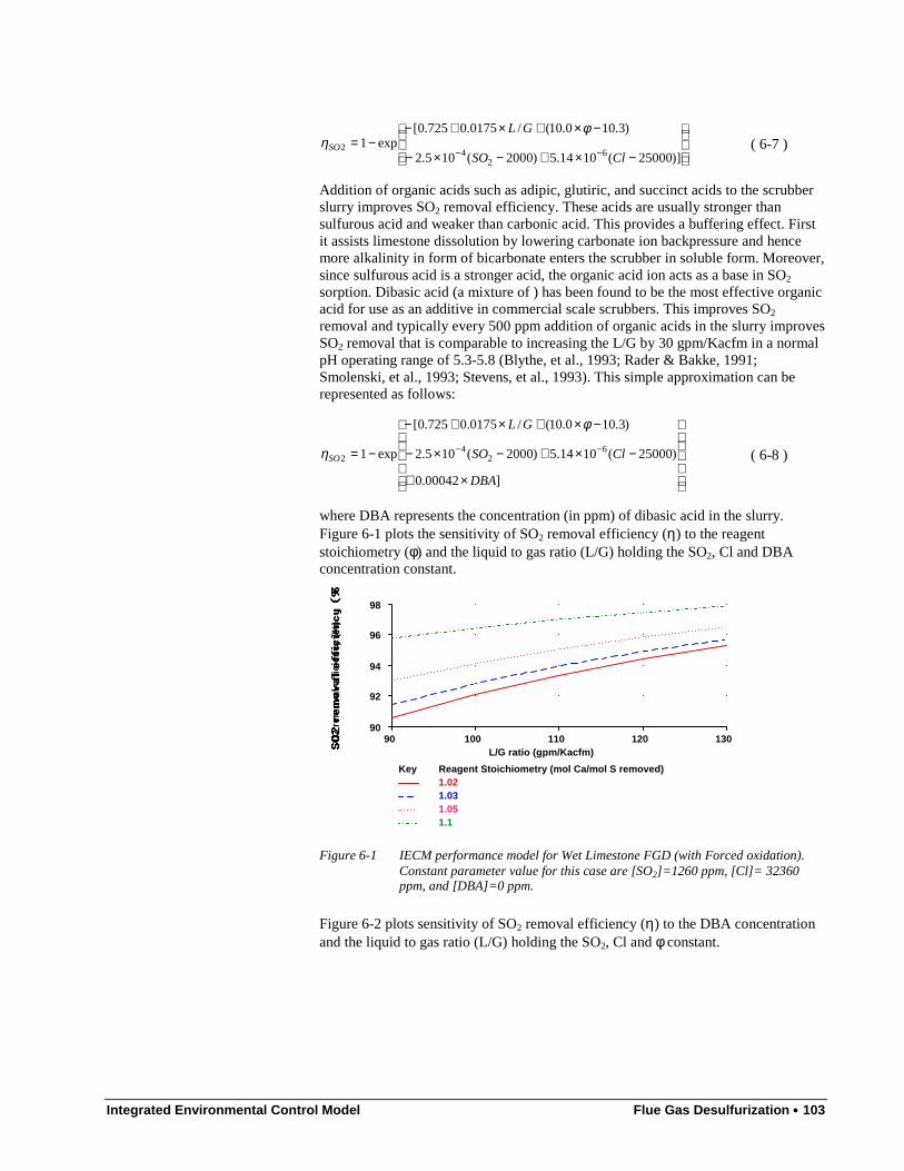
Integrated Environmental Control Model Flue Gas Desulfurization •••• 103
−×+−×−
−×+×+−−=
−− )]25000(1014.5)2000(105.2
)3.100.10(/0175.0725.0[exp1
62
42
ClSO
GLSO
φη ( 6-7 )
Addition of organic acids such as adipic, glutiric, and succinct acids to the scrubberslurry improves SO2 removal efficiency. These acids are usually stronger thansulfurous acid and weaker than carbonic acid. This provides a buffering effect. Firstit assists limestone dissolution by lowering carbonate ion backpressure and hencemore alkalinity in form of bicarbonate enters the scrubber in soluble form. Moreover,since sulfurous acid is a stronger acid, the organic acid ion acts as a base in SO2
sorption. Dibasic acid (a mixture of ) has been found to be the most effective organicacid for use as an additive in commercial scale scrubbers. This improves SO2
removal and typically every 500 ppm addition of organic acids in the slurry improvesSO2 removal that is comparable to increasing the L/G by 30 gpm/Kacfm in a normalpH operating range of 5.3-5.8 (Blythe, et al., 1993; Rader & Bakke, 1991;Smolenski, et al., 1993; Stevens, et al., 1993). This simple approximation can berepresented as follows:
×+
−×+−×−
−×+×+−
−= −−
]00042.0
)25000(1014.5)2000(105.2
)3.100.10(/0175.0725.0[
exp1 62
42
DBA
ClSO
GL
SO
φ
η ( 6-8 )
where DBA represents the concentration (in ppm) of dibasic acid in the slurry.Figure 6-1 plots the sensitivity of SO2 removal efficiency (η) to the reagentstoichiometry (φ) and the liquid to gas ratio (L/G) holding the SO2, Cl and DBAconcentration constant.
SO
2 re
mov
al e
ffici
ency
(%
)
L/G ratio (gpm/Kacfm)90 100 110 120 130
90
92
94
96
98
Key Reagent Stoichiometry (mol Ca/mol S removed)1.021.031.051.1
Figure 6-1 IECM performance model for Wet Limestone FGD (with Forced oxidation).Constant parameter value for this case are [SO2]=1260 ppm, [Cl]= 32360ppm, and [DBA]=0 ppm.
Figure 6-2 plots sensitivity of SO2 removal efficiency (η) to the DBA concentrationand the liquid to gas ratio (L/G) holding the SO2, Cl and φ constant.
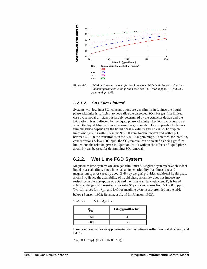
104 •••• Flue Gas Desulfurization Integrated Environmental Control Model
SO
2 re
mov
al e
ffici
ency
(%
)
L/G ratio (gpm/Kacfm)90 100 110 120 130
94
95
96
97
98
99
Key Dibasic Acid Concentration (ppmw)1000150020003000
Figure 6-2 IECM performance model for Wet Limestone FGD (with Forced oxidation).Constant parameter value for this case are [SO2]=1260 ppm, [Cl]= 32360ppm, and φ =1.03.
6.2.1.2. Gas Film LimitedSystems with low inlet SO2 concentrations are gas film limited, since the liquidphase alkalinity is sufficient to neutralize the dissolved SO2. For gas film limitedcase the removal efficiency is largely determined by the contactor design and theL/G ratio; it is not affected by the liquid phase alkalinity. The SO2 concentration atwhich the liquid film resistance becomes large enough to be comparable to the gasfilm resistance depends on the liquid phase alkalinity and L/G ratio. For typicallimestone systems with L/G in the 90-130 gpm/Kacfm interval and with a pHbetween 5.3-5.8 the transition is in the 500-1000 ppm range. Therefore, for inlet SO2
concentrations below 1000 ppm, the SO2 removal can be treated as being gas filmlimited and the relation given in Equation ( 6-1 ) without the effects of liquid phasealkalinity can be used for determining SO2 removal.
6.2.2. Wet Lime FGD SystemMagnesium lime systems are also gas film limited. Maglime systems have abundantliquid phase alkalinity since lime has a higher solubility than limestone andmagnesium species (usually about 2-4% by weight) provides additional liquid phasealkalinity. Hence the availability of liquid phase alkalinity does not impose anyresistance in the absorption of SO2 and the mass transfer coefficient Kg is basedsolely on the gas film resistance for inlet SO2 concentrations from 500-5000 ppm.Typical values for ηSO2
and L/G for maglime systems are provided in the table
below (Benson, 1993; Benson, et al., 1991; Johnson, 1993).
Table 6-5 L/G for Mg-Lime
ηSO2L/G(gpm/Kacfm)
95% 40
98% 56
Based on these values an approximate relation between sulfur removal efficiency andL/G is:
)}/07.02.0(exp{12
GLSO ×+−−=η
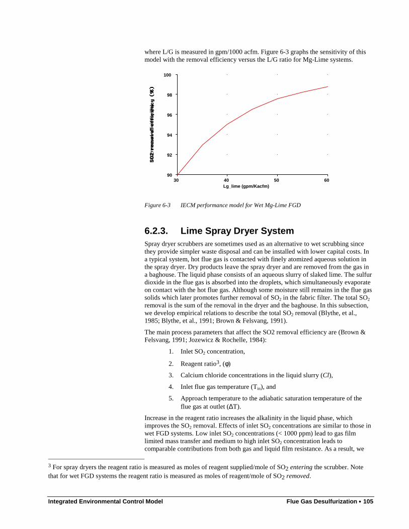
Integrated Environmental Control Model Flue Gas Desulfurization •••• 105
where L/G is measured in gpm/1000 acfm. Figure 6-3 graphs the sensitivity of thismodel with the removal efficiency versus the L/G ratio for Mg-Lime systems.
SO
2 re
mov
al e
ffici
ency
(%
)
Lg_lime (gpm/Kacfm)30 40 50 60
90
92
94
96
98
100
Figure 6-3 IECM performance model for Wet Mg-Lime FGD
6.2.3. Lime Spray Dryer SystemSpray dryer scrubbers are sometimes used as an alternative to wet scrubbing sincethey provide simpler waste disposal and can be installed with lower capital costs. Ina typical system, hot flue gas is contacted with finely atomized aqueous solution inthe spray dryer. Dry products leave the spray dryer and are removed from the gas ina baghouse. The liquid phase consists of an aqueous slurry of slaked lime. The sulfurdioxide in the flue gas is absorbed into the droplets, which simultaneously evaporateon contact with the hot flue gas. Although some moisture still remains in the flue gassolids which later promotes further removal of SO2 in the fabric filter. The total SO2removal is the sum of the removal in the dryer and the baghouse. In this subsection,we develop empirical relations to describe the total SO2 removal (Blythe, et al.,1985; Blythe, et al., 1991; Brown & Felsvang, 1991).
The main process parameters that affect the SO2 removal efficiency are (Brown &Felsvang, 1991; Jozewicz & Rochelle, 1984):
1. Inlet SO2 concentration,
2. Reagent ratio3, (φ)
3. Calcium chloride concentrations in the liquid slurry (Cl),
4. Inlet flue gas temperature (Tin), and
5. Approach temperature to the adiabatic saturation temperature of theflue gas at outlet (∆T).
Increase in the reagent ratio increases the alkalinity in the liquid phase, whichimproves the SO2 removal. Effects of inlet SO2 concentrations are similar to those inwet FGD systems. Low inlet SO2 concentrations (< 1000 ppm) lead to gas filmlimited mass transfer and medium to high inlet SO2 concentration leads tocomparable contributions from both gas and liquid film resistance. As a result, we
3 For spray dryers the reagent ratio is measured as moles of reagent supplied/mole of SO2 entering the scrubber. Notethat for wet FGD systems the reagent ratio is measured as moles of reagent/mole of SO2 removed.
106 •••• Flue Gas Desulfurization Integrated Environmental Control Model
develop different response surfaces to describe the removal efficiency for low andhigh inlet SO2 concentrations. Increasing the inlet temperature allows more water tobe added to the spray dryer to achieve the same approach temperature. This in turnleads to a higher recycle ratio and increased mass transfer area thus improving theremoval efficiency.
In order to understand the effect of the other parameters one has to consider the heattransfer characteristics of the spray dryer. The evaporation time, t, for a given dropletis also the time available for a droplet to absorb SO2. As the approach to saturationtemperature increases, the evaporation time decreases thereby decreasing removalefficiency. The addition of chlorides in the slurry improves the SO2 removalefficiency of the spray dryer. This is due to the deliquescent properties of chlorides,which helps the droplet to retain water and hence increase the evaporation time.Hence chlorides are often used as additives to reduce the lime consumption. We nowdevelop response surfaces to describe the overall SO2 removal efficiency in spraydryers using data from pilot studies conducted by EPRI (1985, 1991) and Joy/Niro(Svend, et al. 1983). We use the log-linear form shown in Equation ( 6-3 ) to developthese response surfaces.
The reagent ratio is a key process variable and it affects the removal efficiencysignificantly. Typical value of SO2 removal for different stochiometries are presentedin Table 6-6 below:
Table 6-6 Reagent Stoichiometry
ηSO2φφφφ
80% 0.9
90% 1.1
These values are representative of both low and high inlet SO2 concentrations. Basedon these numbers the log-linear approximation for the effect of reagent ratio is asfollows:
{ })45.3495.1(exp12 φη ×+−−−=SO ( 6-9 )
This relation can be used for reagent ratios in the range of 0.9-1.8. Now we developthe response surface for low and high SO2 concentrations separately.
6.2.3.1. Low Inlet SO 2 Concentrations ( ≤ 1000 ppm)
The data presented in this section was collected against baseline conditions of 1000ppm inlet SO2, approach temperature of 20°F, and inlet temperature of 280°F. Forlow inlet SO2 concentrations, the inlet temperatures in the range of 280-325°F hasbeen observed to have no effect on the removal efficiency. However increasing theapproach temperature to saturation from 20 to 40°F results in the requirement ofhigher stochiometries for the same removal efficiencies as shown in Table 6-7:
Table 6-7 Effect of 40°F Approach Temperature to Saturation
ηSO2φφφφ
80% 1.1
85% 1.3
Averaging the effects of these values an additional term to describe this effect isadded to Equation ( 6-6 ) as follows:
Integrated Environmental Control Model Flue Gas Desulfurization •••• 107
{ })]20(05.045.3495.1[exp12 −∆×−×+−−−= TSO φη
As discussed earlier the deliquescent properties of calcium chloride improves theremoval efficiency. A presence in the slurry resulting in 0.6% calcium chloride byweight in solids collected in the fabric filter results in higher removal efficiencies forthe same stoichiometry as shown below:
Table 6-8 Effect of 0.6% Calcium Chloride
ηSO2φφφφ
90% 1.0
95% 1.2
Averaging the effects based on these values can be accomplished with additionalterms being added to Equation ( 6-7 ). Thus, the effect of the approach to saturationtemperature and calcium chlorides can be described by Equation ( 6-10 ):
{ }]58.0)20(05.045.3495.1[exp12 ClTSO ×+−∆×−×+−−−= φη ( 6-10 )
This is the final form of the response surface for low SO2 inlet concentrations.
6.2.3.2. Medium to High SO 2 Concentrations (> 1000 ppm)
The data presented in this section was collected against baseline conditions of thefollowing values: 2000 ppm inlet SO2, approach temperature of 20°F, and inlettemperature of 325°F. For inlet SO2 concentrations greater than 1000 ppm, theremoval efficiency increases with increases in inlet temperatures from 280-325°F.Decreasing the inlet temperature to 280°F decreases the removal efficiency to 80%for a given stoichiometry of 1.1. This effect is represented by an additional term toEquation ( 6-9 ) as follows:
{ })]325(015.045.3495.1[exp12 −×+×+−−−= TSO φη
The presence of 0.4% by weight of calcium chloride in the fabric filter solidsprovides an improved efficiency of 90% for a reagent ratio of 1.0. This is describedin by an additional term as follows:
{ }]86.0)325(015.045.3495.1[exp12 ClTSO ×+−×+×+−−−= φη
Increasing the approach temperature to 30°F reduces the removal efficiency to 75%for a reagent ratio of 1.05. On the other hand increasing the inlet SO2 concentrationto 3000 ppm reduces removal efficiency to 80% at a reagent ratio of 1.1. Theseeffects are included as shown below:
−∆×+−×−×+−×+×+−−
−=)]20(08475.0)2000(0007.0
86.0)325(015.045.3495.1[exp1
22 TSO
ClTSO
φη
This is the final form of the response surface for high SO2 inlet concentrations.Figure 6-4 plots the removal efficiency as a function of the inlet flue gas temperaturefor different stochiometries.
Figure 6-5 graphs the sensitivity of the removal efficiency as a function of theapproach temperature for different stochiometries.

108 •••• Flue Gas Desulfurization Integrated Environmental Control Model
SO
2 re
mov
al e
ffici
ency
(%
)
Temp280 290 300 310 320
75
80
85
90
95
Key Msr_dryfgd11.051.11.151.2
Figure 6-4 IECM performance model for Lime Spray Dryer. Constant parameter value forthis case are [Cl]=0.4% wt., [∆T]=28 F, and [SO2]= 1260 ppm
SO
2 re
mov
al e
ffici
ency
(%
)
Dt20 22 24 26 28 30
60
70
80
90
100
Key Msr_dryfgd11.051.11.151.2
Figure 6-5 IECM performance model for Lime Spray Dryer. Constant parameter value forthis case are [Cl]=0.4% wt., [T]=300 F, and [SO2]= 1260 ppm
6.3. FGD Cost ModelsThe FGD cost models originally developed for the IECM were derived from adetailed FGD computer program developed in the late 1970’s and early 1980’s bythe Tennessee Valley Authority (TVA). The TVA model was subjected to anextensive set of parametric runs, and the results were used to derive statistical“response surface” models which accurately represented the results of the TVAmodel in terms of a smaller number of key site-specific plant and design parameters.We follow a similar procedure in developing the new models reported here.
Changes in the design, performance and cost of FGD systems in the mid-to-late1980’s left the TVA model outdated as a basis for performance and cost estimation.The TVA modeling team also was disbanded during this period, and no furtherupdates to the model were made. Instead, the most reliable and widely used estimatesof FGD cost came from a new modeling effort sponsored by the Electric PowerResearch Institute (EPRI). This effort led to the development of a computer modelcalled FGDCOST, which has become the new industry standard in the area.FGDCOST, however, does not contain any FGD performance models (all
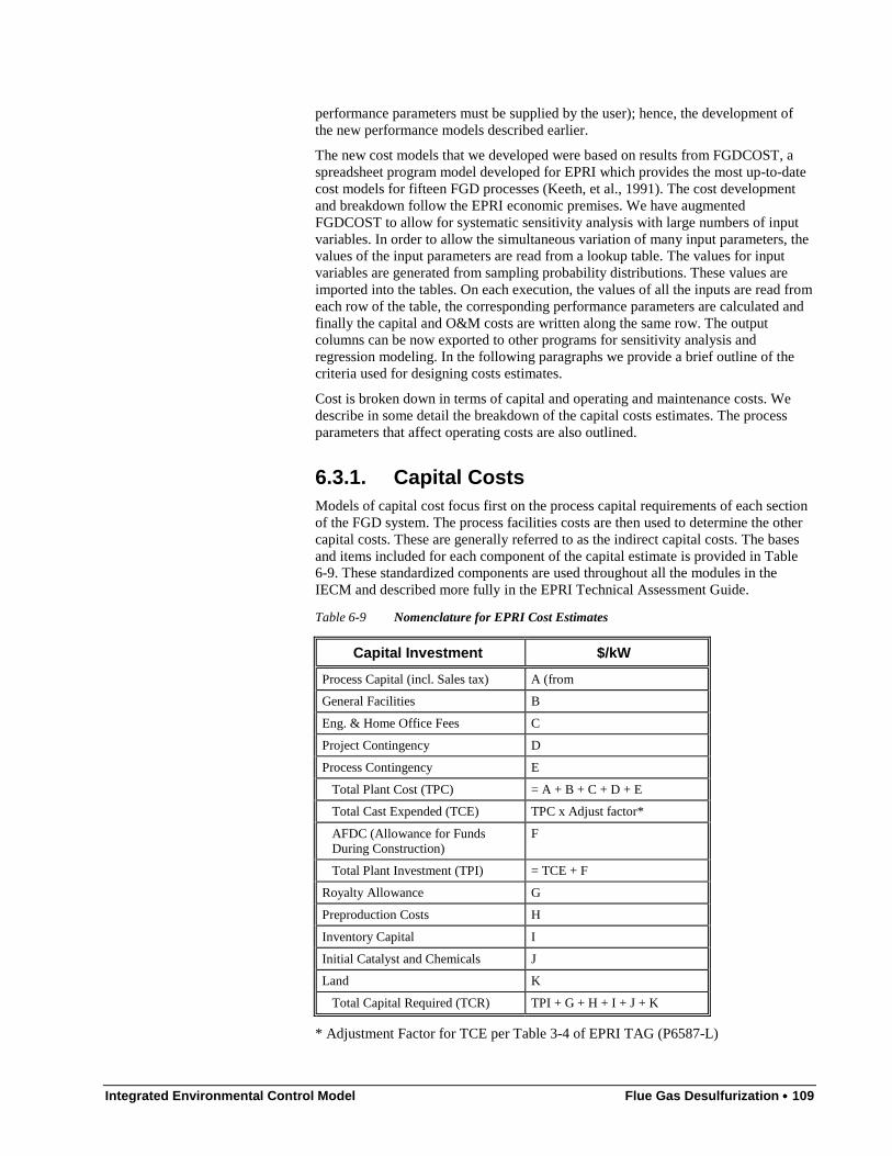
Integrated Environmental Control Model Flue Gas Desulfurization •••• 109
performance parameters must be supplied by the user); hence, the development ofthe new performance models described earlier.
The new cost models that we developed were based on results from FGDCOST, aspreadsheet program model developed for EPRI which provides the most up-to-datecost models for fifteen FGD processes (Keeth, et al., 1991). The cost developmentand breakdown follow the EPRI economic premises. We have augmentedFGDCOST to allow for systematic sensitivity analysis with large numbers of inputvariables. In order to allow the simultaneous variation of many input parameters, thevalues of the input parameters are read from a lookup table. The values for inputvariables are generated from sampling probability distributions. These values areimported into the tables. On each execution, the values of all the inputs are read fromeach row of the table, the corresponding performance parameters are calculated andfinally the capital and O&M costs are written along the same row. The outputcolumns can be now exported to other programs for sensitivity analysis andregression modeling. In the following paragraphs we provide a brief outline of thecriteria used for designing costs estimates.
Cost is broken down in terms of capital and operating and maintenance costs. Wedescribe in some detail the breakdown of the capital costs estimates. The processparameters that affect operating costs are also outlined.
6.3.1. Capital CostsModels of capital cost focus first on the process capital requirements of each sectionof the FGD system. The process facilities costs are then used to determine the othercapital costs. These are generally referred to as the indirect capital costs. The basesand items included for each component of the capital estimate is provided in Table6-9. These standardized components are used throughout all the modules in theIECM and described more fully in the EPRI Technical Assessment Guide.
Table 6-9 Nomenclature for EPRI Cost Estimates
Capital Investment $/kW
Process Capital (incl. Sales tax) A (from
General Facilities B
Eng. & Home Office Fees C
Project Contingency D
Process Contingency E
Total Plant Cost (TPC) = A + B + C + D + E
Total Cast Expended (TCE) TPC x Adjust factor*
AFDC (Allowance for Funds During Construction)
F
Total Plant Investment (TPI) = TCE + F
Royalty Allowance G
Preproduction Costs H
Inventory Capital I
Initial Catalyst and Chemicals J
Land K
Total Capital Required (TCR) TPI + G + H + I + J + K
* Adjustment Factor for TCE per Table 3-4 of EPRI TAG (P6587-L)
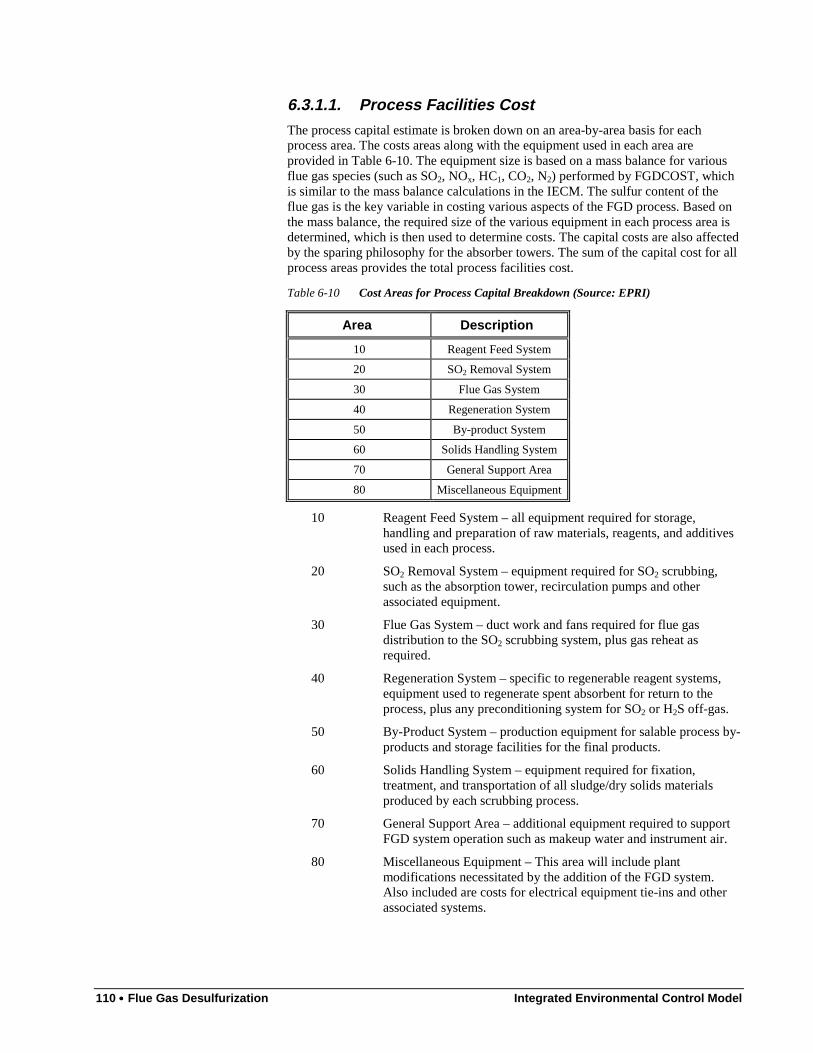
110 •••• Flue Gas Desulfurization Integrated Environmental Control Model
6.3.1.1. Process Facilities CostThe process capital estimate is broken down on an area-by-area basis for eachprocess area. The costs areas along with the equipment used in each area areprovided in Table 6-10. The equipment size is based on a mass balance for variousflue gas species (such as SO2, NOx, HC1, CO2, N2) performed by FGDCOST, whichis similar to the mass balance calculations in the IECM. The sulfur content of theflue gas is the key variable in costing various aspects of the FGD process. Based onthe mass balance, the required size of the various equipment in each process area isdetermined, which is then used to determine costs. The capital costs are also affectedby the sparing philosophy for the absorber towers. The sum of the capital cost for allprocess areas provides the total process facilities cost.
Table 6-10 Cost Areas for Process Capital Breakdown (Source: EPRI)
Area Description
10 Reagent Feed System
20 SO2 Removal System
30 Flue Gas System
40 Regeneration System
50 By-product System
60 Solids Handling System
70 General Support Area
80 Miscellaneous Equipment
10 Reagent Feed System – all equipment required for storage,handling and preparation of raw materials, reagents, and additivesused in each process.
20 SO2 Removal System – equipment required for SO2 scrubbing,such as the absorption tower, recirculation pumps and otherassociated equipment.
30 Flue Gas System – duct work and fans required for flue gasdistribution to the SO2 scrubbing system, plus gas reheat asrequired.
40 Regeneration System – specific to regenerable reagent systems,equipment used to regenerate spent absorbent for return to theprocess, plus any preconditioning system for SO2 or H2S off-gas.
50 By-Product System – production equipment for salable process by-products and storage facilities for the final products.
60 Solids Handling System – equipment required for fixation,treatment, and transportation of all sludge/dry solids materialsproduced by each scrubbing process.
70 General Support Area – additional equipment required to supportFGD system operation such as makeup water and instrument air.
80 Miscellaneous Equipment – This area will include plantmodifications necessitated by the addition of the FGD system.Also included are costs for electrical equipment tie-ins and otherassociated systems.
Integrated Environmental Control Model Flue Gas Desulfurization •••• 111
6.3.1.2. Other Capital Costs:Besides the process capital costs, a series of additional indirect costs are included inthe IECM cost models. Following the EPRI format, these are represented as simpleparameters whose values are user-specified. Their relationship to each other and tothe direct facilities cost are shown in Table 6-9.
General Facilities: The general facilities costs include roads, office buildings,shops, laboratories etc. A cost factor (fgf) of 5 - 20% of the processcapital cost is used to evaluate this cost. A cost factor of fgf=10% isused as default value in the FGDCOST models.
Engineering & Home Office Fees: An estimate of engineering, home officeoverhead and fees is included in capital costs estimates. A costfactor (feho) of about 10 -15% is used to estimate this expense.FGDCOST uses a value of f eho=10% of the process facilities cost.
Project Contingency: Project contingency costs covers additional equipment andother costs that would arise from a more detailed design. Projectcontingency factors (fcproj) range from 10 - 20% of process capitalcosts. An average value of about 15% is used in FGDCOST.
Process Contingency: A process contingency is applied to a new technology inan attempt to quantify the design uncertainty and the cost of acommercial scale system. The contingency factor (fcproc) can rangefrom 2-50% of the process capital costs. For FGD processes acontingency factor of 2% is used.
Total Plant Cost: The total plant cost (tpc) is the sum of process capital, generalfacilities, engineering and home office fees, and contingencies.
Total Cash Expended: The total cash expended is an estimate of the cashexpected to be spend during the construction duration of the FGDsystem. This estimate accounts only for the escalation of costs upto the date of expenditure.
Allowance for Funds During Construction (AFUDC): The schedule forengineering procurement and construction is assumed to be twoyears for installation. For example, for an escalation of 5% a year,the total plant costs is multiplied by 0.0548 to calculate theallowance for interest expenses during a two year constructionperiod. The IECM has general function which calculates theescalation costs given the escalation rate and the time forinstallation.
Total Plant Investment: The total plant investment is the sum of the total cashexpended and the allowance for interest during construction.
Royalty Allowance: Royalties paid are 0.5% of the process capital.
Preproduction Costs: Preproduction costs are intended to cover operatortraining, equipment checkout, major changes in plant equipment,extra maintenance, and inefficient use of materials during plantstartup. It is a sum of one-month fixed operating costs, one-monthvariable operating costs at full capacity and 2% of the total plantinvestment.
Inventory Capital: The inventory costs includes the expense of raw materialsand other consumables based on a 100% capacity operation for 60days.

112 •••• Flue Gas Desulfurization Integrated Environmental Control Model
Land: FGD system land requirements include the plant site area anddisposal area. Land has not been included as a line item.
Total Capital Requirement: The total capital requirement is calculated as thetotal of all the costs enumerated above.
6.3.1.3. Operating & Maintenance CostsOperating costs for FGD systems are separated into fixed and variable operatingcosts. Fixed costs include operating and maintenance labor, maintenance materialsand administrative/support labor. Various factors based on EPRI premises are usedto estimate these costs many of which are based on capital cost estimates. Variableoperating costs include consumables such as fuel, water, power, chemicals, andsolids disposal. Error! Not a valid bookmark self-reference. provides theoperating cost criteria used. The fixed and variable O&M costs depend on the feedrate of reagent, sludge disposal costs, power for pumping, labor and other operations.Table 6-12 provides the default process design criteria used in our models.
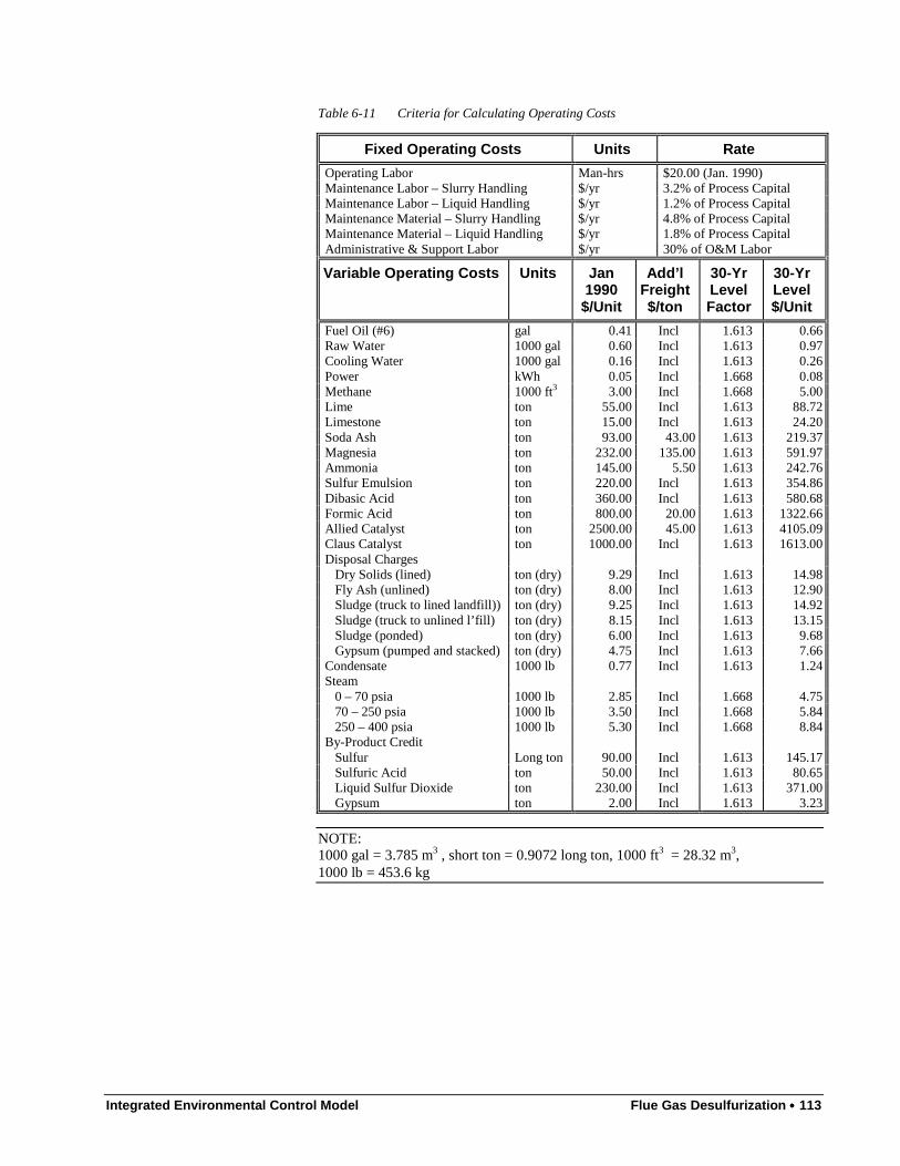
Integrated Environmental Control Model Flue Gas Desulfurization •••• 113
Table 6-11 Criteria for Calculating Operating Costs
Fixed Operating Costs Units Rate
Operating Labor Man-hrs $20.00 (Jan. 1990)Maintenance Labor – Slurry Handling $/yr 3.2% of Process CapitalMaintenance Labor – Liquid Handling $/yr 1.2% of Process CapitalMaintenance Material – Slurry Handling $/yr 4.8% of Process CapitalMaintenance Material – Liquid Handling $/yr 1.8% of Process CapitalAdministrative & Support Labor $/yr 30% of O&M Labor
Variable Operating Costs Units Jan1990$/Unit
Add’lFreight$/ton
30-YrLevelFactor
30-YrLevel$/Unit
Fuel Oil (#6) gal 0.41 Incl 1.613 0.66Raw Water 1000 gal 0.60 Incl 1.613 0.97Cooling Water 1000 gal 0.16 Incl 1.613 0.26Power kWh 0.05 Incl 1.668 0.08Methane 1000 ft3 3.00 Incl 1.668 5.00Lime ton 55.00 Incl 1.613 88.72Limestone ton 15.00 Incl 1.613 24.20Soda Ash ton 93.00 43.00 1.613 219.37Magnesia ton 232.00 135.00 1.613 591.97Ammonia ton 145.00 5.50 1.613 242.76Sulfur Emulsion ton 220.00 Incl 1.613 354.86Dibasic Acid ton 360.00 Incl 1.613 580.68Formic Acid ton 800.00 20.00 1.613 1322.66Allied Catalyst ton 2500.00 45.00 1.613 4105.09Claus Catalyst ton 1000.00 Incl 1.613 1613.00Disposal Charges Dry Solids (lined) ton (dry) 9.29 Incl 1.613 14.98 Fly Ash (unlined) ton (dry) 8.00 Incl 1.613 12.90 Sludge (truck to lined landfill)) ton (dry) 9.25 Incl 1.613 14.92 Sludge (truck to unlined l’fill) ton (dry) 8.15 Incl 1.613 13.15 Sludge (ponded) ton (dry) 6.00 Incl 1.613 9.68 Gypsum (pumped and stacked) ton (dry) 4.75 Incl 1.613 7.66Condensate 1000 lb 0.77 Incl 1.613 1.24Steam 0 – 70 psia 1000 lb 2.85 Incl 1.668 4.75 70 – 250 psia 1000 lb 3.50 Incl 1.668 5.84 250 – 400 psia 1000 lb 5.30 Incl 1.668 8.84By-Product Credit Sulfur Long ton 90.00 Incl 1.613 145.17 Sulfuric Acid ton 50.00 Incl 1.613 80.65 Liquid Sulfur Dioxide ton 230.00 Incl 1.613 371.00 Gypsum ton 2.00 Incl 1.613 3.23
NOTE:1000 gal = 3.785 m3 , short ton = 0.9072 long ton, 1000 ft3 = 28.32 m3,1000 lb = 453.6 kg

114 •••• Flue Gas Desulfurization Integrated Environmental Control Model
Table 6-12 Description of Default Criteria used in the Model
Variablename
Units Description DefaultValue
gas Kacfm flue gas flow rate 971MW 106 MW Net plant capacity 300
L/G gpm/Kacfm liquid to gas ratio 90/55/30a
%S % % sulfur in coal by weight 2.6%1750 ppm
stoichiometry(φ)
moles of Ca per mole of SO2 removed 1.03/1.02/ 1.1b
labor $/hr FGD operating labor rate 20reag $/ton reagent (CaCO3/CaO) cost 15/55d
solid $/ton sludge disposal cost 8.15stack $/ton sludge disposal - stacking cost 4.75power mills/kWh power cost 50steam $/1000 lbs steam cost 3.5waterf $/1000 gallons fresh water cost 0.6waterc $/1000 gallons cooling water cost 0.16
DBAppm* ppm scrubber slurry DBA concentration 1500
DBAfeed* lbs DBA/ton
SO2 removedDBA feed rate 20
DBAcostc $/ton DBA additive cost 360
∆P inches of H2O total system pressure drop 10
∆T •F temperature increase of scrubbed fluegas due to reheat
25
a the default values are: 90 gpm/Kacfm for LSFO and 55 gpm/Kacfm for LSDBA and 30for Mg-lime System for a 90% removal efficiency.
B the stoichiometry for limestone systems is 1.03, for lime systems is 1.02, and for limespray dryer is 1.1(note that for lime spray dryer the reported stoichiometry is moles of Caper mole of inlet SO2).
C these input variables for LS/DBA only
d limestone cost is 15 and lime cost is 55 $/ton
6.3.2. The Methodological ApproachResponse surface construction is the central objective of the sensitivity analysistechniques presented in this section. Sensitivity analysis seeks to identify the set ofinput variables that have significant effect on the model output and to rank orderthem according to the magnitude of their effects. Once the relevant variables areidentified regression methods can be used to develop adequate response surfacereplacements for the models. Subsequently probability distributions on the inputvariables can be used in conjunction with the response surface to derive theprobability distributions of the model outputs. In this section, we briefly describe theuse of Latin hypercube sampling (LHS) (Iman, et al., 1980) along with partial rankcorrelation coefficients (PRCC) to examine the influence of individual variables onthe model output (Iman, et al., 1981a; Iman, et al., 1981b). Finally the use ofregression analysis with log-linear transformations for developing response surfacesis described (Ang & Tang, 1975; Draper & Smith, 1966; Neter, et al., 1983).

Integrated Environmental Control Model Flue Gas Desulfurization •••• 115
6.3.2.1. Sampling and Ranking MethodsIn order to perform sensitivity analysis it is necessary to obtain model output forvarious values of input variables. Latin hypercube sampling is used to select valuesfor input variables. The LHS technique to select n different values from k differentinput variables operates in the following manner. For each variable, the range isdivided into n non-overlapping intervals of equal probability. One value from eachinterval is selected at random with respect to the probability density in the interval.The n values for variable x1 are paired at random with the n values of x2 and these npairs are paired at random with n values of x3 and so on to generate n k-tuples. Thisis the Latin hypercube sample used as input to the model. The model is thenexercised at each of these n input values to generate n l-tuples for l output variablesof interest. This data set of n k-tuples of input values and n l-tuple of output valuesforms the basis for the rest of the analysis.
The importance of an input variable is derived by assessing its influence on theoutput variable. For linear relationships this can be assessed by the use of partialcorrelation coefficients (PCC) which measure the correlation between an input andoutput variable when the effects of all the other variables is removed. For nonlinearrelations it becomes more difficult to assess the importance of individual variables.However, if the model output is a monotonic function of the input then it is possibleto linearize the relationship by using rank transformations on the input and outputvalues. A rank transformation involves replacing each value of a variable by its rank.Now the partial correlation coefficient on the rank transformed variables (PRCC) canbe used to assess the importance of the input variables.
6.3.2.2. Regression AnalysisOnce the important input variables are chosen, multivariate linear regressionapproaches can be used with the data set to construct response surfaces. If k inputvariables are chosen as relevant, a linear regression model is written as:
ε+++++= kki xbxbxbay ...2211
where, ε is an error term which represents the variance in yi unexplained by themodel. The linear fit is obtained by selecting a, bi so as to minimize the sum ofsquares between the model predictions and the data for yi. Often the relationshipsbetween input and output variables are nonlinear. In this case it is often possible touse some data transformation to linearize the relationship. A commonly usedtransformation for exponential nonlinearities is the logarithm transform. Thereforean exponential relationship such as:
kbk
bbi xxxay ×××= ...21
21
is transformed to:
)ln(...)ln()ln()ln( 11 kki xbxbay +++=
which has a linear relationship.
Common statistical tests are used to determine the adequacy of the regression model.The most common measure is the coefficient of multiple correlation (R2) which is aratio of the variation explained by the regression to the total variation in yi. Values ofR2 near 1 represent good fits. R2 however is not a sufficient measure of the goodnessof fit of a model. The t-statistic is used to test if the partial regression coefficients a,bi are significantly different from zero. Moreover an F-statistic can be used to checkif any of the partial correlation coefficients are different from zero. This statisticprovides an idea of the lack of fit of a regression model as a whole. However, for
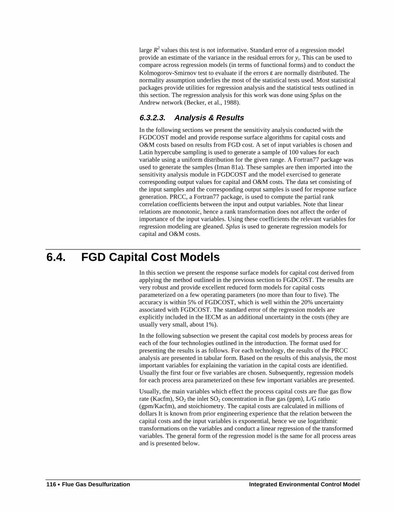
116 •••• Flue Gas Desulfurization Integrated Environmental Control Model
large R2 values this test is not informative. Standard error of a regression modelprovide an estimate of the variance in the residual errors for yi. This can be used tocompare across regression models (in terms of functional forms) and to conduct theKolmogorov-Smirnov test to evaluate if the errors ε are normally distributed. Thenormality assumption underlies the most of the statistical tests used. Most statisticalpackages provide utilities for regression analysis and the statistical tests outlined inthis section. The regression analysis for this work was done using Splus on theAndrew network (Becker, et al., 1988).
6.3.2.3. Analysis & ResultsIn the following sections we present the sensitivity analysis conducted with theFGDCOST model and provide response surface algorithms for capital costs andO&M costs based on results from FGD cost. A set of input variables is chosen andLatin hypercube sampling is used to generate a sample of 100 values for eachvariable using a uniform distribution for the given range. A Fortran77 package wasused to generate the samples (Iman 81a). These samples are then imported into thesensitivity analysis module in FGDCOST and the model exercised to generatecorresponding output values for capital and O&M costs. The data set consisting ofthe input samples and the corresponding output samples is used for response surfacegeneration. PRCC, a Fortran77 package, is used to compute the partial rankcorrelation coefficients between the input and output variables. Note that linearrelations are monotonic, hence a rank transformation does not affect the order ofimportance of the input variables. Using these coefficients the relevant variables forregression modeling are gleaned. Splus is used to generate regression models forcapital and O&M costs.
6.4. FGD Capital Cost ModelsIn this section we present the response surface models for capital cost derived fromapplying the method outlined in the previous section to FGDCOST. The results arevery robust and provide excellent reduced form models for capital costsparameterized on a few operating parameters (no more than four to five). Theaccuracy is within 5% of FGDCOST, which is well within the 20% uncertaintyassociated with FGDCOST. The standard error of the regression models areexplicitly included in the IECM as an additional uncertainty in the costs (they areusually very small, about 1%).
In the following subsection we present the capital cost models by process areas foreach of the four technologies outlined in the introduction. The format used forpresenting the results is as follows. For each technology, the results of the PRCCanalysis are presented in tabular form. Based on the results of this analysis, the mostimportant variables for explaining the variation in the capital costs are identified.Usually the first four or five variables are chosen. Subsequently, regression modelsfor each process area parameterized on these few important variables are presented.
Usually, the main variables which effect the process capital costs are flue gas flowrate (Kacfm), SO2 the inlet SO2 concentration in flue gas (ppm), L/G ratio(gpm/Kacfm), and stoichiometry. The capital costs are calculated in millions ofdollars It is known from prior engineering experience that the relation between thecapital costs and the input variables is exponential, hence we use logarithmictransformations on the variables and conduct a linear regression of the transformedvariables. The general form of the regression model is the same for all process areasand is presented below.
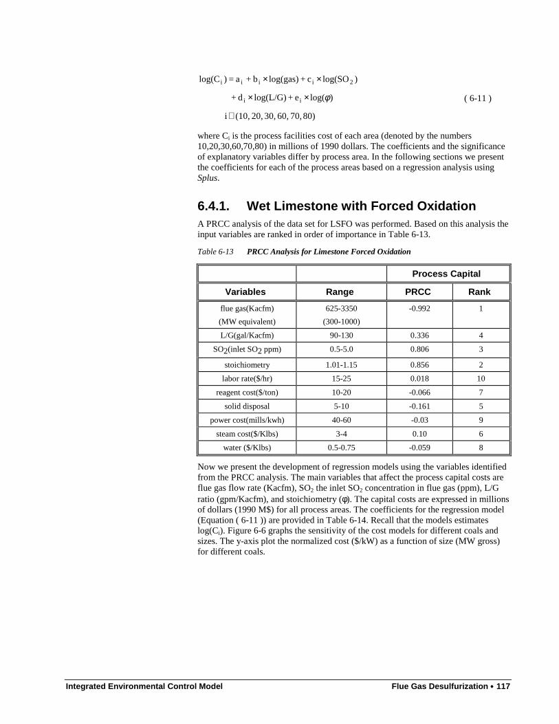
Integrated Environmental Control Model Flue Gas Desulfurization •••• 117
80) 70, 60, 30, 20, (10, i
)log(e + log(L/G)d +
)log(SOc + log(gas)b + a = )log(C
ii
2iiii
∈
××
××
φ ( 6-11 )
where Ci is the process facilities cost of each area (denoted by the numbers10,20,30,60,70,80) in millions of 1990 dollars. The coefficients and the significanceof explanatory variables differ by process area. In the following sections we presentthe coefficients for each of the process areas based on a regression analysis usingSplus.
6.4.1. Wet Limestone with Forced OxidationA PRCC analysis of the data set for LSFO was performed. Based on this analysis theinput variables are ranked in order of importance in Table 6-13.
Table 6-13 PRCC Analysis for Limestone Forced Oxidation
Process Capital
Variables Range PRCC Rank
flue gas(Kacfm)
(MW equivalent)
625-3350
(300-1000)
-0.992 1
L/G(gal/Kacfm) 90-130 0.336 4
SO2(inlet SO2 ppm) 0.5-5.0 0.806 3
stoichiometry 1.01-1.15 0.856 2
labor rate($/hr) 15-25 0.018 10
reagent cost($/ton) 10-20 -0.066 7
solid disposal 5-10 -0.161 5
power cost(mills/kwh) 40-60 -0.03 9
steam cost($/Klbs) 3-4 0.10 6
water ($/Klbs) 0.5-0.75 -0.059 8
Now we present the development of regression models using the variables identifiedfrom the PRCC analysis. The main variables that affect the process capital costs areflue gas flow rate (Kacfm), SO2 the inlet SO2 concentration in flue gas (ppm), L/Gratio (gpm/Kacfm), and stoichiometry (φ). The capital costs are expressed in millionsof dollars (1990 M$) for all process areas. The coefficients for the regression model(Equation ( 6-11 )) are provided in Table 6-14. Recall that the models estimateslog(Ci). Figure 6-6 graphs the sensitivity of the cost models for different coals andsizes. The y-axis plot the normalized cost ($/kW) as a function of size (MW gross)for different coals.
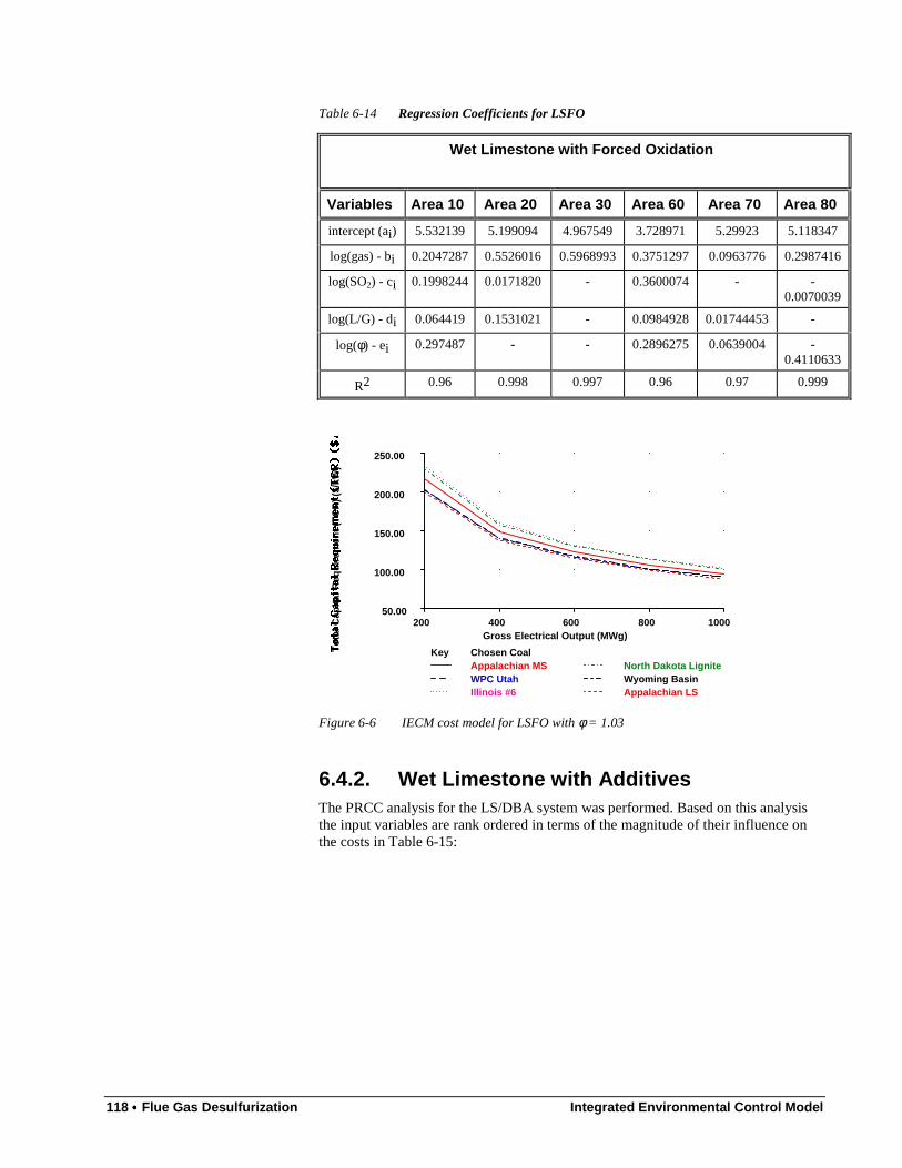
118 •••• Flue Gas Desulfurization Integrated Environmental Control Model
Table 6-14 Regression Coefficients for LSFO
Wet Limestone with Forced Oxidation
Variables Area 10 Area 20 Area 30 Area 60 Area 70 Area 80
intercept (ai) 5.532139 5.199094 4.967549 3.728971 5.29923 5.118347
log(gas) - bi 0.2047287 0.5526016 0.5968993 0.3751297 0.0963776 0.2987416
log(SO2) - ci 0.1998244 0.0171820 - 0.3600074 - -0.0070039
log(L/G) - di 0.064419 0.1531021 - 0.0984928 0.01744453 -
log(φ) - ei 0.297487 - - 0.2896275 0.0639004 -0.4110633
R2 0.96 0.998 0.997 0.96 0.97 0.999
Tot
al C
apita
l Req
uire
men
t (T
CR
) ($
/kW
)
Gross Electrical Output (MWg)200 400 600 800 1000
50.00
100.00
150.00
200.00
250.00
Key Chosen CoalAppalachian MSWPC UtahIllinois #6
North Dakota LigniteWyoming BasinAppalachian LS
Figure 6-6 IECM cost model for LSFO with φ = 1.03
6.4.2. Wet Limestone with AdditivesThe PRCC analysis for the LS/DBA system was performed. Based on this analysisthe input variables are rank ordered in terms of the magnitude of their influence onthe costs in Table 6-15:

Integrated Environmental Control Model Flue Gas Desulfurization •••• 119
Table 6-15 PRCC analysis for Wet Limestone with Dibasic Acid
Capital Costs
Variables Range PRCC Rank
flue gas(Kacfm)
size (MW)
625-3350
(300-1000)
-0.991 1
L/G(gpm/Kacfm) 50-90 0.293 4
%S(weight) 0.5-5.0 0.803 3
stoichiometry 1.01-1.15 0.852 2
labor rate($/hr) 15-25 0.071 9
reagent cost($/ton) 10-20 -0.031 11
solid disposal 5-10 -0.173 6
power cost(mills/kwh) 40-60 0.056 10
steam cost($/Klbs) 3-4 0.192 5
water fresh($/Klbs) 0.5-0.75 -0.073 8
DBA ppm 1-2K 0 12
DBA feed (lbs/ton of SO2) 15-25 -0.147 7
DBA cost($/ton) 300-400 0 12
Now we present the development of regression models using the variables identifiedby the PRCC analysis. The regression analysis is parallel to the one presented forLSFO with a data set that is different, i.e. generated using a cost model for LS/DBA.The main variables which affect the process capital costs (expressed in 1990 M$) areflue gas flow rate (Kacfm), SO2 in inlet flue gas, L/G ratio (gpm/Kacfm), andstoichiometry (φ). Note that the range of L/G for LS/DBA is between 60-90. Onceagain using logarithmic transformations, linear regressions (Equation ( 6-11 )) areused for each process area. We provide highlights for each process area in Table6-16. Figure 6-7 graphs the sensitivity of the normalized cost ($/kW) for differentcoals and sizes (MW gross).
Table 6-16 Regression Coefficients for Wet Limestone with DBA
Wet Limestone with DBA
ModelParameter
Area 10 Area 20 Area 30 Area 60 Area 70 Area 80
intercept (ai) 5.656823 5.283843 4.967474 3.914778 5.33193 5.118347
log(gas) - bi 0.2116698 0.5487767 0.5969214 0.3830471 0.0932564 0.2987416
log(SO2) - ci 0.1965567 0.0182601 - 0.3528121 0.0033284 -0.0070039
log(L/G) - di - 0.1124185 - - - -
log(φ) - ei 0.3971839 - - 0.6173974 0.0825347 -0.4110633
R2 0.96 0.998 0.997 0.95 0.98 0.999

120 •••• Flue Gas Desulfurization Integrated Environmental Control Model
Tot
al C
apita
l Req
uire
men
t (T
CR
) ($
/kW
)
Gross Electrical Output (MWg)200 400 600 800 1000
50.00
100.00
150.00
200.00
250.00
Key Chosen CoalAppalachian MSWPC UtahIllinois #6
North Dakota LigniteWyoming BasinAppalachian LS
Figure 6-7 IECM cost model for Wet Limestone FGD with 1500 ppm of DBA as additive.
6.4.3. Magnesium-Enhanced Lime SystemA PRCC analysis of the data set for Mg-Lime system was performed. Based on thisanalysis the input variables are ranked in order of importance in Table 6-17.
Table 6-17 PRCC Analysis for Mg-Lime
Process Capital
Variables Range PRCC Rank
flue gas(Kacfm)
(MW equivalent)
625-3350
(300-1000)
-0.986 1
L/G(gal/Kacfm) 30-56 0.149 4
SO2(inlet SO2 ppm) 0.5-5.0 0.890 2
stoichiometry 1.01-1.15 0.801 3
labor rate($/hr) 15-25 0.13 6
reagent cost($/ton) 50-60 -0.069 8
solid disposal 5-10 -0.133 5
power cost(mills/kwh) 40-60 -0.051 10
steam cost($/Klbs) 3-4 0.064 9
water ($/Klbs) 0.5-0.75 -0.097 7
Now we present the development of regression models using the variables identifiedfrom the PRCC analysis. The main variables which affect the process capital costsare flue gas flow rate (Kacfm), SO2 the inlet SO2 concentration in flue gas (ppm),L/G ratio (gpm/Kacfm), and stoichiometry. The results are deduced from aregression analysis based on Equation ( 6-11 ) using Splus. The highlights arepresented in Table 6-18. Figure 6-8 graphs the sensitivity of the normalized cost($/kW) for different coals and sizes (MW gross).

Integrated Environmental Control Model Flue Gas Desulfurization •••• 121
Table 6-18 Regression Coefficients for Process Facilities Capital Cost
Wet Limestone with Mg-Lime
Area 10 Area 20 Area 30 Area 60 Area 70 Area 80
intercept (ai) 4.18205 5.343637 4.985706 3.805031 5.406733 5.118347
log(gas) - bi 0.4287465 0.5571364 0.5965417 0.4408358 0.0859990 0.2987416
log(SO2) - ci 0.3973585 -0.0031376 -0.0057330 0.4067988 -0.0042571 -0.0070039
log(L/G) - di - 0.0865696 - - - -
log(φ) - ei - - - - 0.0711735 -0.4110633
R2 0.96 0.999 0.999 0.97 0.98 0.999
Tot
al C
apita
l Req
uire
men
t (T
CR
) ($
/kW
)
Gross Electrical Output (MWg)200 400 600 800 1000
75.00
100.00
125.00
150.00
175.00
200.00
Key Chosen CoalAppalachian MSWPC UtahIllinois #6
North Dakota LigniteWyoming BasinAppalachian LS
Figure 6-8 IECM cost model for Mg-enhanced Lime FGD with φ = 1.02
6.4.4. Lime Spray DryerA PRCC analysis of the data set for the Lime Spray Dryer was performed. Based onthis analysis the input variables are ranked in order of importance in the table below.Note however, that some of the key operating parameters are different for the LimeSpray Dryer. The water entering with the slurry spray vaporizes and the flue gas(along with the fly ash) carries the dried reaction products. These particles are thenremoved in the baghouse (downstream of the FGD) and a portion of the collectedsolids is recycled back to the absorber. The amount of recycle (lb of dry solidsrecycled/lb of lime added) is based on the sulfur content of the flue gas. The totalslurry that is recycled to the absorber (gpm) depends on the recycle ratio (rr),stoichiometric ratio (φ) and the flue gas flow rate (gas). In order to determine thegpm we need to solve the process flowsheet of the LSD iteratively. In order to avoidthis computational burden for the IECM we have developed a regression equation forthe slurry flow rate as a function the recycle ratio, stoichiometry and the flue gasflow rate as shown below.
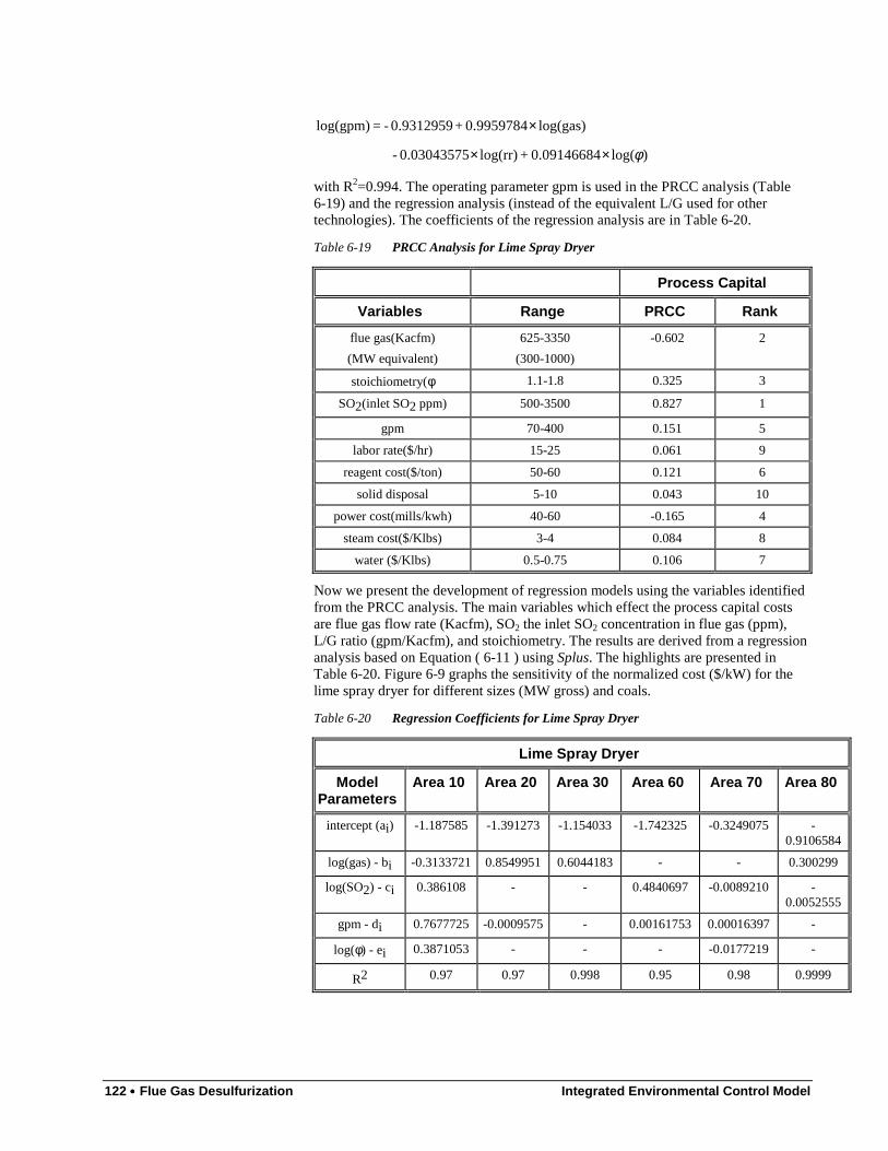
122 •••• Flue Gas Desulfurization Integrated Environmental Control Model
)log(0.09146684 + log(rr)0.03043575 -
log(gas)0.9959784+0.9312959- = log(gpm)
φ××
×
with R2=0.994. The operating parameter gpm is used in the PRCC analysis (Table6-19) and the regression analysis (instead of the equivalent L/G used for othertechnologies). The coefficients of the regression analysis are in Table 6-20.
Table 6-19 PRCC Analysis for Lime Spray Dryer
Process Capital
Variables Range PRCC Rank
flue gas(Kacfm)
(MW equivalent)
625-3350
(300-1000)
-0.602 2
stoichiometry(φ 1.1-1.8 0.325 3
SO2(inlet SO2 ppm) 500-3500 0.827 1
gpm 70-400 0.151 5
labor rate($/hr) 15-25 0.061 9
reagent cost($/ton) 50-60 0.121 6
solid disposal 5-10 0.043 10
power cost(mills/kwh) 40-60 -0.165 4
steam cost($/Klbs) 3-4 0.084 8
water ($/Klbs) 0.5-0.75 0.106 7
Now we present the development of regression models using the variables identifiedfrom the PRCC analysis. The main variables which effect the process capital costsare flue gas flow rate (Kacfm), SO2 the inlet SO2 concentration in flue gas (ppm),L/G ratio (gpm/Kacfm), and stoichiometry. The results are derived from a regressionanalysis based on Equation ( 6-11 ) using Splus. The highlights are presented inTable 6-20. Figure 6-9 graphs the sensitivity of the normalized cost ($/kW) for thelime spray dryer for different sizes (MW gross) and coals.
Table 6-20 Regression Coefficients for Lime Spray Dryer
Lime Spray Dryer
ModelParameters
Area 10 Area 20 Area 30 Area 60 Area 70 Area 80
intercept (ai) -1.187585 -1.391273 -1.154033 -1.742325 -0.3249075 -0.9106584
log(gas) - bi -0.3133721 0.8549951 0.6044183 - - 0.300299
log(SO2) - ci 0.386108 - - 0.4840697 -0.0089210 -0.0052555
gpm - di 0.7677725 -0.0009575 - 0.00161753 0.00016397 -
log(φ) - ei 0.3871053 - - - -0.0177219 -
R2 0.97 0.97 0.998 0.95 0.98 0.9999

Integrated Environmental Control Model Flue Gas Desulfurization •••• 123
Tot
al C
apita
l Req
uire
men
t (T
CR
) ($
/kW
)
Gross Electrical Output (MWg)200 400 600 800 1000
50.00
75.00
100.00
125.00
150.00
175.00
Key Chosen CoalAppalachian MSWPC UtahIllinois #6
North Dakota LigniteWyoming BasinAppalachian LS
Figure 6-9 IECM cost model for Lime Spray Dryer for φ = 1.1
6.4.5. Sparing PhilosophyThe models developed in the previous subsections are based on the assumption oftwo operating absorber towers (each rated at 50% of the plant capacity, with amaximum of 650MW) and one spare absorber tower. With the recent development ofadvanced absorber towers of near 100% reliability it is possible to eliminate thespare tower and reduce capital costs significantly (no significant changes in variablecosts). Another approach to reducing capital cost exploits the economy of scale byusing single absorber towers of large capacity. In this subsection we develop scalingfactors to estimate the reduction in capital costs for different FGD systems bychanging the sparing philosophy. Note that in all the factors developed below, thescaling factors are derived by a regression of the capital cost of various sparingphilosophies against the capital cost of the default system, i.e. an FGD with twooperating towers and one spare absorber.
In order to estimate the reduction in capital costs from eliminating the spare tower,we set the number of spare towers in FGDCOST to zero and exercise the model forvarious values of input for the relevant variables such as flue gas flow rate (gas), SO2
in flue gas, L/G, and stoichiometry (φ). The capital costs for system with no spares(C') is then regressed against the capital cost for the system with one spare tower (C)and correlation coefficient (si) of this regression provides us with the scaling factorwe desire:
30) (20, i ,C s = C ii/i ∈×
where Ci is the process area (denoted by 20, 30) cost. The capital cost of the SO2
removal system (includes absorber towers) and the flue gas system (includes pipingto absorber towers) is affected by the sparing philosophy. We present results forthose process areas whose capital cost is affected in Table 6-21. The columns under"Zero Sparing" characterize the reduction in capital cost by dropping the spareabsorber. The columns under "One Absorber" characterize the reduction in capitalcost by reducing the number of absorbers from two (rated @50% each) to one (rated@100% of capacity).
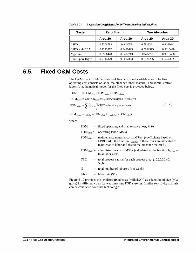
124 •••• Flue Gas Desulfurization Integrated Environmental Control Model
Table 6-21 Regression Coefficients for Different Sparing Philosophies
System Zero Sparing One Absorber
Area 20 Area 30 Area 20 Area 30
LSFO 0.7306793 0.943658 0.5818281 0.9449641
LSFO with DBA 0.7213572 0.9436423 0.5692575 0.9316498
Mg-Lime 0.6926448 0.9437713 0.525391 0.9316498
Lime Spray Dryer 0.7114379 0.8002883 0.5126236 0.64543523
6.5. Fixed O&M CostsThe O&M costs for FGD consists of fixed costs and variable costs. The fixedoperating cost consists of labor, maintenance labor, material, and administrativelabor. A mathematical model for the fixed cost is provided below.
( )
)FOMf + (FOMf =FOM
area process = i whereTPCf FOM
(weeks/yr) 52 (hrs/week) 40 N labor FOM
FOMFOMFOM = FOM
maintmaintlablaboradminadmin
imaintmaint
laborlabor
adminmaintlabor
××
×=
×××=
++
∑ii
( 6-12 )
where
FOM = fixed operating and maintenance cost, M$/yr
FOMlabor = operating labor, M$/yr
FOMmaint = maintenance material costs, M$/yr, (coefficients based onEPRI TAG, the fraction fmaintlab of these costs are allocated tomaintenance labor and rest to maintenance material).
FOMadmin = administrative costs, M$/yr (calculated as the fraction f2admin oftotal labor costs)
TPCi = total process capital for each process area, (10,20,30,40,50,60)
N = total number of laborers (per week)
labor = labor rate ($/hr)
Figure 6-10 provides the levelized fixed costs (mills/kWh) as a function of size (MWgross) for different coals for wet limestone FGD systems. Similar sensitivity analysiscan be conducted for other technologies.
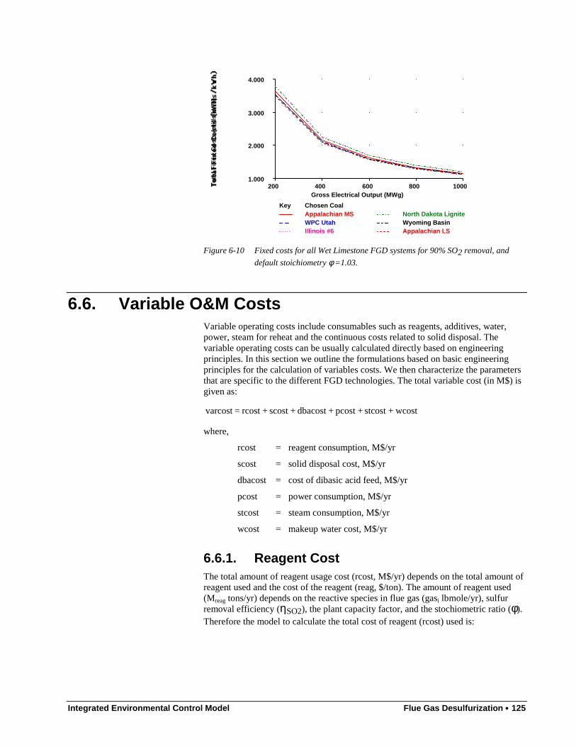
Integrated Environmental Control Model Flue Gas Desulfurization •••• 125
Tot
al F
ixed
Cos
ts (
mill
s/kW
h)
Gross Electrical Output (MWg)200 400 600 800 1000
1.000
2.000
3.000
4.000
Key Chosen CoalAppalachian MSWPC UtahIllinois #6
North Dakota LigniteWyoming BasinAppalachian LS
Figure 6-10 Fixed costs for all Wet Limestone FGD systems for 90% SO2 removal, and
default stoichiometry φ =1.03.
6.6. Variable O&M CostsVariable operating costs include consumables such as reagents, additives, water,power, steam for reheat and the continuous costs related to solid disposal. Thevariable operating costs can be usually calculated directly based on engineeringprinciples. In this section we outline the formulations based on basic engineeringprinciples for the calculation of variables costs. We then characterize the parametersthat are specific to the different FGD technologies. The total variable cost (in M$) isgiven as:
wcost+stcost +pcost +dbacost +scost +rcost =varcost
where,
rcost = reagent consumption, M$/yr
scost = solid disposal cost, M$/yr
dbacost = cost of dibasic acid feed, M$/yr
pcost = power consumption, M$/yr
stcost = steam consumption, M$/yr
wcost = makeup water cost, M$/yr
6.6.1. Reagent CostThe total amount of reagent usage cost (rcost, M$/yr) depends on the total amount ofreagent used and the cost of the reagent (reag, $/ton). The amount of reagent used(Mreag tons/yr) depends on the reactive species in flue gas (gasi lbmole/yr), sulfurremoval efficiency (ηSO2), the plant capacity factor, and the stochiometric ratio (φ).Therefore the model to calculate the total cost of reagent (rcost) used is:

126 •••• Flue Gas Desulfurization Integrated Environmental Control Model
purityCaCOiireag
reag
R/8766cfMW)rgas( 2000
1= M
Mreag =rcost
3
××××××
×
∑i
ii φη( 6-13 )
where
i ∈ (SO2, SO3, HCl)
ri = moles of reagent required per mole of species, I
ri ∈ (1, 1, ½)
3CaCOMW = molecular weight of CaCO3
Rpurity = reagent purity (weight fraction of CaCO3)
6.6.2. Solid Waste Disposal CostsThe solid waste disposal cost (scost, M$/yr) depends on the amount of solid wasteand the unit cost of disposal (disposal, in $/ton). The amount of solid waste produceddepends on the amount of reactive species scrubbed from the flue gas (Mdisposal
tons/yr), the total amount of inerts in the slurry (Minerts, tons/yr) and the amount ofunused reagent in the slurry (Munused reagent, tons/yr). Therefore the model to calculatethe total cost of waste disposal (scost) is:
( )
( )
( )( )
∑
∑
−
×××−×××
×=
××−×=
×××××××=
++×=
8766)1(
2000
1
876612000
87662000
1
3
cos
cfR
MrgasM
cfRM
M
cfMWrgasM
MMMdisposals
purity
CaCOiiiireagunused
purityreag
inerts
iiiiiidisposal
gunused reainertsdisposalt
φη
φη
( 6-14 )
where,
i ∈ (SO2, SO3, HCl)
ri = moles of reagent required per mole of species
ri ∈ (1, 1, ½)
MWi =( )( )
••
••
System Lime ,,
System Limestone ,,
22323
22424
55
22
CaClOHCaSOOHCaSO
CaClOHCaSOOHCaSO
MWMWMW
MWMWMW
6.6.3. Power CostsThe power costs (pcost, M$/yr) depends on the unit cost of power (power, $/MWh),and power consumption in the reagent handling (P20, MW) and flue gas handlingsystems (P30, MW). Slurry is injected into the absorber towers at four levels toremove SO2 and a pump serves each level. The power consumption for these pumpsis proportional to the amount of slurry being pumped (Q, gallons/hr) and the total
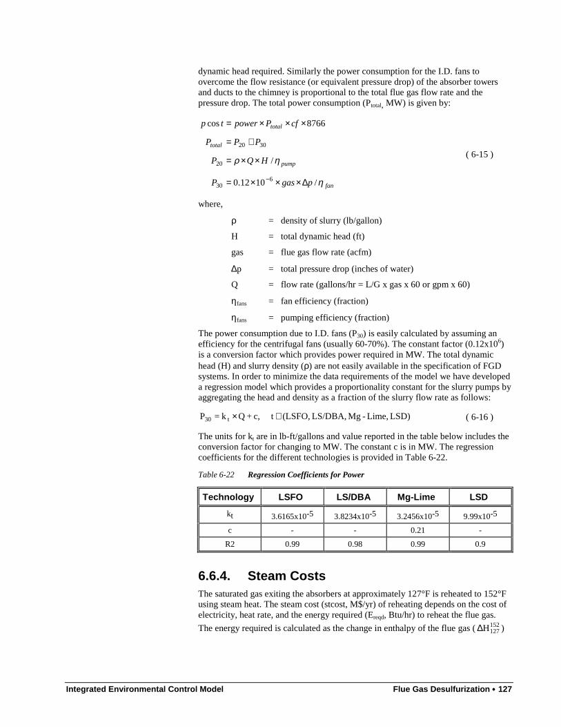
Integrated Environmental Control Model Flue Gas Desulfurization •••• 127
dynamic head required. Similarly the power consumption for the I.D. fans toovercome the flow resistance (or equivalent pressure drop) of the absorber towersand ducts to the chimney is proportional to the total flue gas flow rate and thepressure drop. The total power consumption (Ptotal, MW) is given by:
fan
pump
total
total
pgasP
HQP
PPP
cfPpowertp
η
ηρ
/1012.0
/
8766cos
630
20
3020
∆×××=
××=
+=
×××=
−
( 6-15 )
where,
ρ = density of slurry (lb/gallon)
H = total dynamic head (ft)
gas = flue gas flow rate (acfm)
∆p = total pressure drop (inches of water)
Q = flow rate (gallons/hr = L/G x gas x 60 or gpm x 60)
ηfans = fan efficiency (fraction)
ηfans = pumping efficiency (fraction)
The power consumption due to I.D. fans (P30) is easily calculated by assuming anefficiency for the centrifugal fans (usually 60-70%). The constant factor (0.12x10⁶)is a conversion factor which provides power required in MW. The total dynamichead (H) and slurry density (ρ) are not easily available in the specification of FGDsystems. In order to minimize the data requirements of the model we have developeda regression model which provides a proportionality constant for the slurry pumps byaggregating the head and density as a fraction of the slurry flow rate as follows:
LSD) Lime,-Mg LS/DBA, (LSFO, tc, + Qk = P t30 ∈× ( 6-16 )
The units for kt are in lb-ft/gallons and value reported in the table below includes theconversion factor for changing to MW. The constant c is in MW. The regressioncoefficients for the different technologies is provided in Table 6-22.
Table 6-22 Regression Coefficients for Power
Technology LSFO LS/DBA Mg-Lime LSD
kt 3.6165x10⁻⁵ 3.8234x10⁻⁵ 3.2456x10⁻⁵ 9.99x10⁻⁵
c - - 0.21 -
R2 0.99 0.98 0.99 0.9
6.6.4. Steam CostsThe saturated gas exiting the absorbers at approximately 127°F is reheated to 152°Fusing steam heat. The steam cost (stcost, M$/yr) of reheating depends on the cost ofelectricity, heat rate, and the energy required (Ereqd, Btu/hr) to reheat the flue gas.
The energy required is calculated as the change in enthalpy of the flue gas (152127H∆ )

128 •••• Flue Gas Desulfurization Integrated Environmental Control Model
and the heat of vaporization for the water removed (vaporH∆ ). IECM calculates all
the necessary thermodynamic relationships and properties.
vapor152127reqd H + H = E ∆∆ ( 6-17 )
The cost of reheating is calculated by estimating the cost of the equivalent electricitythat could have been generated if the steam had not been used for reheating:
8766cfpower/hrE =stcost reqd ××× ( 6-18 )
where hr is the steam cycle heat rate (Btu/kWh) and power is the cost of electricity($/kWh).
6.6.5. DBA CostsFor systems that use organic acid additives (LS/DBA), the cost of replacing DBAwhich degrades on a yearly basis (dbacost, M$/yr) depends on the replacement costof Dibasic Acid (CDBA, $/ton), and the amount of DBA degradation (FDBA, tons/yr),which depends on the amount of SO2 removed (MSO2, tons/yr) and the degradation ofDBA per ton of SO2 removed (DDBA, lb of DBA/ton of SO2 removed). This ischaracterized as follows:
8766cfTD2000
1 = F
8766cf)Mgas( 2000
1 = M
FC =dbacost
2
2222
SODBADBA
SOSOSOSO
DBADBA
××××
×××××
×
η
6.6.6. Water CostsWater from the scrubbing slurry is lost due to evaporation in the scrubber. The watercosts pertain to the supply needed to replenish this loss. The water cost (wcost,M$/yr) depends on the cost of fresh water (waterf, $/Kgallons), and the total amountof water used (Wtotal, Kgallons). The water costs are characterized as:
lhoursannuaMW60 W= W
W00 waterf/10=wcost
grossMWtotal
total
×××
×( 6-19 )
where WMW is the water consumed (gallons/min) per MW gross. This consumptiondiffers for different technologies. Nominal values used for model development areshown in Table 6-23.
Table 6-23 Water Consumption for FGD Systems
Technology LSFO LS/DBA Mg-Lime LSD
WMW (gpm/MW) 0.098 0.098 1.08 -
Figure 6-11 graphs the total levelized variable O&M costs (mills/kWh) as a functionof size (MW gross) and coal type for Wet Limestone FGD. Similar analysis can beconducted for different technologies.
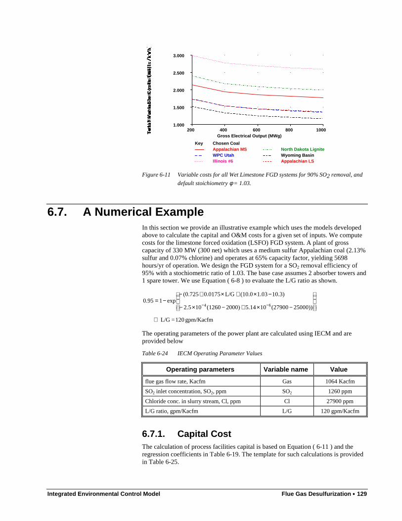
Integrated Environmental Control Model Flue Gas Desulfurization •••• 129
Tot
al V
aria
ble
Cos
ts (
mill
s/kW
h)
Gross Electrical Output (MWg)200 400 600 800 1000
1.000
1.500
2.000
2.500
3.000
Key Chosen CoalAppalachian MSWPC UtahIllinois #6
North Dakota LigniteWyoming BasinAppalachian LS
Figure 6-11 Variable costs for all Wet Limestone FGD systems for 90% SO2 removal, and
default stoichiometry φ = 1.03.
6.7. A Numerical ExampleIn this section we provide an illustrative example which uses the models developedabove to calculate the capital and O&M costs for a given set of inputs. We computecosts for the limestone forced oxidation (LSFO) FGD system. A plant of grosscapacity of 330 MW (300 net) which uses a medium sulfur Appalachian coal (2.13%sulfur and 0.07% chlorine) and operates at 65% capacity factor, yielding 5698hours/yr of operation. We design the FGD system for a SO2 removal efficiency of95% with a stochiometric ratio of 1.03. The base case assumes 2 absorber towers and1 spare tower. We use Equation ( 6-8 ) to evaluate the L/G ratio as shown.
gpm/Kacfm 120 =L/G
25000))(27900105.142000)(1260102.5
10.3)1.03(10.0L/G0.0175(0.725exp195.0
64
⇒
−×+−×−
−×+×+−−=
−−
The operating parameters of the power plant are calculated using IECM and areprovided below
Table 6-24 IECM Operating Parameter Values
Operating parameters Variable name Value
flue gas flow rate, Kacfm Gas 1064 Kacfm
SO2 inlet concentration, SO2, ppm SO2 1260 ppm
Chloride conc. in slurry stream, Cl, ppm Cl 27900 ppm
L/G ratio, gpm/Kacfm L/G 120 gpm/Kacfm
6.7.1. Capital CostThe calculation of process facilities capital is based on Equation ( 6-11 ) and theregression coefficients in Table 6-19. The template for such calculations is providedin Table 6-25.
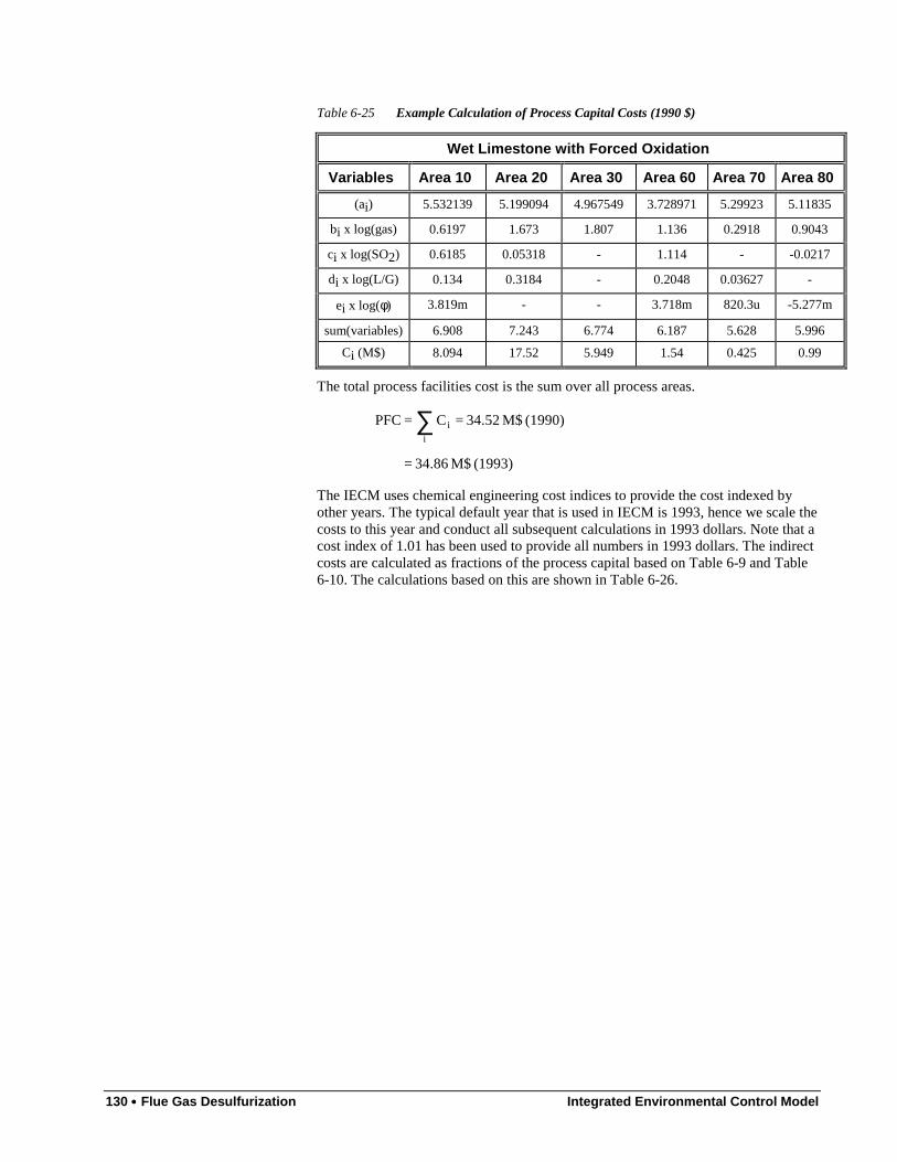
130 •••• Flue Gas Desulfurization Integrated Environmental Control Model
Table 6-25 Example Calculation of Process Capital Costs (1990 $)
Wet Limestone with Forced Oxidation
Variables Area 10 Area 20 Area 30 Area 60 Area 70 Area 80
(ai) 5.532139 5.199094 4.967549 3.728971 5.29923 5.11835
bi x log(gas) 0.6197 1.673 1.807 1.136 0.2918 0.9043
ci x log(SO2) 0.6185 0.05318 - 1.114 - -0.0217
di x log(L/G) 0.134 0.3184 - 0.2048 0.03627 -
ei x log(φ) 3.819m - - 3.718m 820.3u -5.277m
sum(variables) 6.908 7.243 6.774 6.187 5.628 5.996
Ci (M$) 8.094 17.52 5.949 1.54 0.425 0.99
The total process facilities cost is the sum over all process areas.
(1993) M$ 34.86 =
(1990) M$ 34.52 = C = PFCi
i∑
The IECM uses chemical engineering cost indices to provide the cost indexed byother years. The typical default year that is used in IECM is 1993, hence we scale thecosts to this year and conduct all subsequent calculations in 1993 dollars. Note that acost index of 1.01 has been used to provide all numbers in 1993 dollars. The indirectcosts are calculated as fractions of the process capital based on Table 6-9 and Table6-10. The calculations based on this are shown in Table 6-26.
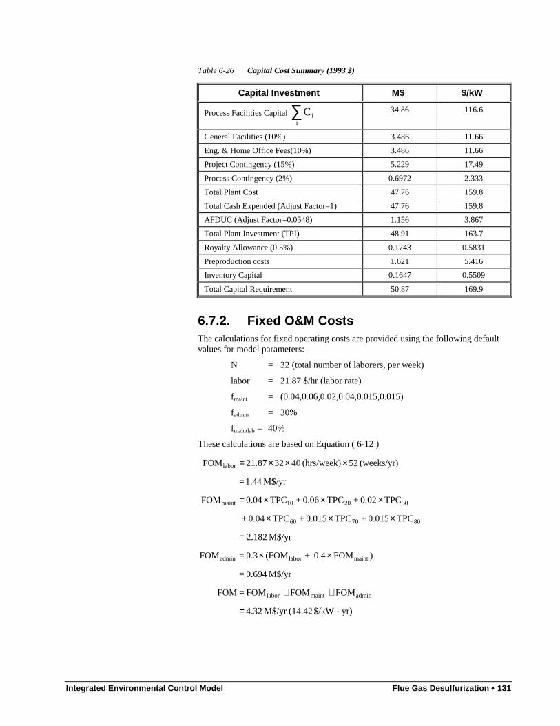
Integrated Environmental Control Model Flue Gas Desulfurization •••• 131
Table 6-26 Capital Cost Summary (1993 $)
Capital Investment M$ $/kW
Process Facilities Capital Cii
∑ 34.86 116.6
General Facilities (10%) 3.486 11.66
Eng. & Home Office Fees(10%) 3.486 11.66
Project Contingency (15%) 5.229 17.49
Process Contingency (2%) 0.6972 2.333
Total Plant Cost 47.76 159.8
Total Cash Expended (Adjust Factor=1) 47.76 159.8
AFDUC (Adjust Factor=0.0548) 1.156 3.867
Total Plant Investment (TPI) 48.91 163.7
Royalty Allowance (0.5%) 0.1743 0.5831
Preproduction costs 1.621 5.416
Inventory Capital 0.1647 0.5509
Total Capital Requirement 50.87 169.9
6.7.2. Fixed O&M CostsThe calculations for fixed operating costs are provided using the following defaultvalues for model parameters:
N = 32 (total number of laborers, per week)
labor = 21.87 $/hr (labor rate)
fmaint = (0.04,0.06,0.02,0.04,0.015,0.015)
fadmin = 30%
fmaintlab = 40%
These calculations are based on Equation ( 6-12 )
yr)-$/kW (14.42M$/yr 4.32
FOMFOMFOM = FOM
M$/yr 0.694 =
)FOM0.4 + (FOM0.3 =FOM
M$/yr 182.2
TPC0.015 +TPC0.015 +TPC0.04 +
TPC0.02 + TPC0.06 + TPC0.04 FOM
M$/yr 1.44=
(weeks/yr) 52 (hrs/week) 40 23 21.87 FOM
admin maintlabor
maintlaboradmin
807060
302010maint
labor
=
++
××
=
×××
×××=
×××=

132 •••• Flue Gas Desulfurization Integrated Environmental Control Model
6.7.3. Variable O&M CostsThe calculations for variable operating costs are providing using the followingdefault values for model parameters:
η = 95% (SO2 removal efficiency)
φ = 1.03 (reagent stoichiometry)
gasSO2 = 140.8 (lb moles/hr, IECM calculation)
gasSO3 = 1.63 (lb moles/hr, IECM calculation)
gasHCl = 8.67 (lb moles/hr, IECM calculation)
152127H∆ = 19.7 MBtu/hr (IECM calculation)
vaporH∆ = 1.24 MBtu/hr (IECM calculation)
reag = 15 $/ton (reagent cost)
cf = 65% (capacity factor)
Rpurity = 94% (reagent purity, wt. fraction)
3CaCOMW = 100 (molecular weight)
O2HCaSO 24MW • =172 (molecular weight)
2CaClMW = 112 (molecular weight)
6.7.3.1. Reagent CostThis calculation is based on Equation ( 6-13 )
M$ 0.671 = T15.15 =rcost
K26.44
94.0/5698001
)0.5(HCl) 67.80.195.0(
+ )1)(SO 1.630.195.0(
+ )1)(SO 140.803.195.0(
2000
1= T
reag
3
2
reag
×
=
××
×××
×××
×××
∑i
6.7.3.2. Solid Waste Disposal CostsThis calculation is based on Equation ( 6-14 )
Integrated Environmental Control Model Flue Gas Desulfurization •••• 133
( ) M$ 0.605 =
M + M +M8.15 =scost
(tons/yr)K 1.238 =
94.0/5698001
)0.5(HCl) 67.80.1)0.10.1(9.0(
+ )1)(SO 1.63)0.10.1(9.0(
+ )1)(SO 140.8)103.1(9.0(
2000
1 = M
(tons/yr)3.365K =
)/200094.01(44.26K = M
(tons/yr)69.63K
5698
)1120.5(HCl) 67.80.19.0(
+ )1721)(SO 1.630.19.0(
+ )1721)(SO 140.803.19.0(
2000
1 = M
reagent unusedinertsdisposal
3
2
reagent unused
inerts
3
2
disposal
×
××
××−×
××−×
××−×
×
−×
=
×
××××
××××
××××
×
∑
∑
i
i
6.7.3.3. Power CostsThis calculation is based on Equations ( 6-15 ) and ( 6-16 )
M$ 1.78 = 5698P43.45 =pcost
MW 5.73 = P + P = P
MW 2.56 = /0.5101064100.12 = P
MW 3.34 = 0 + 1064120103.62 = P
total
3020total
6-30
-520
××
×××
×××
6.7.3.4. Steam CostsThis calculation is based on Equations ( 6-17 ) and ( 6-18 )
M$ 0.665 = 698545.431K/788020.94 =stcost
(MBtu/hr) 20.94 =
MBtu/hr) ,H( 1.24 + MBtu/hr) ,H( 19.7 = E vapor152127reqd
×××
∆∆
6.7.3.5. Water CostsThis calculation is based on Equation ( 6-19 )
mills/kWh) 10(4.53$/yr 7721 =
Wgallons)($/K 0.7 =wcost
earKgallons/y 11.06 = 6985603030.098 = W
3-
total
total
×
×
×××
6.7.3.6. Total Variable Operating CostsThe total variable costs (mills/kWh) are derived as the sum of the reagent, solidwaste disposal, power and steam costs as follows:
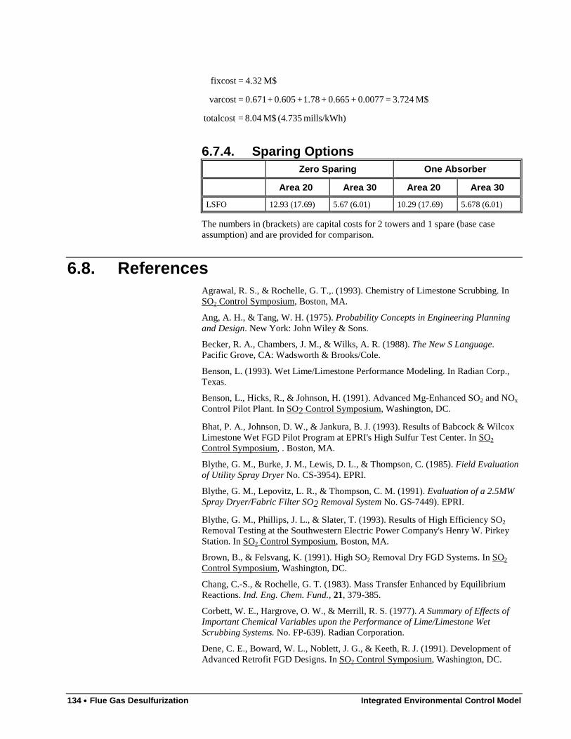
134 •••• Flue Gas Desulfurization Integrated Environmental Control Model
mills/kWh) (4.735 M$ 8.04 =totalcost
M$ 3.724 = 0.0077 + 0.665 + 1.78 + 0.605 + 0.671 =varcost
M$ 4.32 =fixcost
6.7.4. Sparing OptionsZero Sparing One Absorber
Area 20 Area 30 Area 20 Area 30
LSFO 12.93 (17.69) 5.67 (6.01) 10.29 (17.69) 5.678 (6.01)
The numbers in (brackets) are capital costs for 2 towers and 1 spare (base caseassumption) and are provided for comparison.
6.8. ReferencesAgrawal, R. S., & Rochelle, G. T.,. (1993). Chemistry of Limestone Scrubbing. InSO2 Control Symposium, Boston, MA.
Ang, A. H., & Tang, W. H. (1975). Probability Concepts in Engineering Planningand Design. New York: John Wiley & Sons.
Becker, R. A., Chambers, J. M., & Wilks, A. R. (1988). The New S Language.Pacific Grove, CA: Wadsworth & Brooks/Cole.
Benson, L. (1993). Wet Lime/Limestone Performance Modeling. In Radian Corp.,Texas.
Benson, L., Hicks, R., & Johnson, H. (1991). Advanced Mg-Enhanced SO2 and NOx
Control Pilot Plant. In SO2 Control Symposium, Washington, DC.
Bhat, P. A., Johnson, D. W., & Jankura, B. J. (1993). Results of Babcock & WilcoxLimestone Wet FGD Pilot Program at EPRI's High Sulfur Test Center. In SO2
Control Symposium, . Boston, MA.
Blythe, G. M., Burke, J. M., Lewis, D. L., & Thompson, C. (1985). Field Evaluationof Utility Spray Dryer No. CS-3954). EPRI.
Blythe, G. M., Lepovitz, L. R., & Thompson, C. M. (1991). Evaluation of a 2.5MWSpray Dryer/Fabric Filter SO2 Removal System No. GS-7449). EPRI.
Blythe, G. M., Phillips, J. L., & Slater, T. (1993). Results of High Efficiency SO2
Removal Testing at the Southwestern Electric Power Company's Henry W. PirkeyStation. In SO2 Control Symposium, Boston, MA.
Brown, B., & Felsvang, K. (1991). High SO2 Removal Dry FGD Systems. In SO2
Control Symposium, Washington, DC.
Chang, C.-S., & Rochelle, G. T. (1983). Mass Transfer Enhanced by EquilibriumReactions. Ind. Eng. Chem. Fund., 21, 379-385.
Corbett, W. E., Hargrove, O. W., & Merrill, R. S. (1977). A Summary of Effects ofImportant Chemical Variables upon the Performance of Lime/Limestone WetScrubbing Systems. No. FP-639). Radian Corporation.
Dene, C. E., Boward, W. L., Noblett, J. G., & Keeth, R. J. (1991). Development ofAdvanced Retrofit FGD Designs. In SO2 Control Symposium, Washington, DC.
Integrated Environmental Control Model Flue Gas Desulfurization •••• 135
Draper, N. R., & Smith, H. (1966). Applied Regression Analysis. New York: JohnWiley & Sons.
Iman, R. L., Davenport, J. M., & Zeigler, D. K. (1980). Latin Hypercube Sampling(A Program User's Guide). No. SAND79-1473). Sandia National Laboratories.
Iman, R. L., Helton, J. C., & Campbell, J. E. (1981a). An Approach to SensitivityAnalysis of Computer Models: Part I - Introduction, Input Variable Selection andPreliminary Variable Assessment. Journal of Quality Technology, 13(3), 174-183.
Iman, R. L., Helton, J. C., & Campbell, J. E. (1981b). An Approach to SensitivityAnalysis of Computer Models: Part II - Ranking of Input Variables, ResponseSurface Validation, Distribution Effect and Technique Synopsis. Journal of QualityTechnology, 13(4), 232-40.
Johnson, H. (1993). Advanced Mg-Enhanced Wet FGDs. In
Jozewicz, W., & Rochelle, G. T. (1984). Modeling of SO2 Removal by Spray Dryers.In Pittsburgh Coal Technology Conference, Pittsburgh, PA.
Keeth, R. J., Baker, D. L., Tracy, P. E., Ogden, G. E., & Ireland, P. A. (1991).Economic Evaluation of Flue Gas Desulfurization Systems No. GS-7193, ResearchProject 1610-6.). EPRI, Palo Alto, CA.
Klingspor, J. (1993). Wet Limestone Modeling. In ABB Environmental Systems.
Laslow, D. (1993). Wet Lime/Limestone Performance Modeling. In GeneralElectric, Connecticut.
Mehta, R. R., & Rochelle, G. T. (1983). Modeling of SO2 Removal and LimestoneUtilization in Slurry Scrubbing with Forced Oxidation. In AIChE National Meeting,Houston, TX.
Moser, R. E., & Owens, D. R. (1990). Overview on the Use of Additives in WetFGD Systems. In SO2 Control Symposium, New Orleans, LA.
Neter, J., Wasserman, W., & Kutner, M. H. (1983). Applied Linear Regression.Homewood, ILL: R.D. Irwin.
Noblett Jr., G. E., DeKraker, D. P., & Moser, R. E. (1990). FGDPRISM, EPRI'sFGD Process Model -- Recent Applications. In SO2 Control Symposium, NewOrleans, LA.
Noblett Jr., G. E., Hebets, M. J., & Moser, R. E. (1990). EPRI's FGD Process Model(FGDPRISM). In 1990 SO2 Control Symposium, Washington, DC.
Noblett Jr., J. (1993). Wet Lime/Limestone Performance Modeling. In Radian Corp.,Texas.
Rader, P. (1993). Wet Limestone Modeling. In ABB Environmental Systems.
Rader, P. C., & Bakke, E. (1991). Incorporating Full-Scale Experience intoAdvanced Limestone Wet FGD Designs. In 1991 SO2 Control Symposium,Washington, DC.
Rochelle, G. T. (1981). Appendix A: Chemistry of Limestone Scrubbing. In R. H.Borgwardt (Eds.), Limestone FGD Scrubbers: Users Handbook EPA.
Rochelle, G. T. (1981). Appendix B: Operational Factors of Limestone Scrubbing. InR. H. Borgwardt (Eds.), Limestone FGD Scrubbers: Users Handbook EPA.
Smolenski, J., Phillips, J. L., Epsenscheid, A. P., & Shires, T. M. (1993). HighEfficiency SO2 Removal Tests at Tampa Electric Company's Big Bend Unit 4. InSO2 Control Symposium, Boston, MA.

136 •••• Flue Gas Desulfurization Integrated Environmental Control Model
Stevens, G. E., Horton, W. M., Hargrove, O. W., & Owens, D. R. (1993). Evaluationof High SO2 Removal Efficiency Upgrade Options: EPRI High Sulfur Test Center.In SO2 Control Symposium, Boston, MA.
Stevens, G. E., Sitkiewitz, S. S., Phillips, J. L., & Owens, D. R. (1991). Results ofHigh SO2 Removal Efficiency Tests at EPRI's High Sulfur Test Center. In SO2
Control Symposium, Washington, DC.
Weilert, C. (1993). Wet Lime/Limestone Performance Modeling. In Burns andMcDonnell, Missouri.
Weilert, C. V., & Ratliff, J. (1990). Development and Use of Site-Specific FGDSystem Performance and Economic Models. In SO2 Control Symposium, NewOrleans, LA: EPRI/EPA.
Integrated Environmental Control Model Fluidized Bed Copper Oxide Process •••• 137
7. Fluidized Bed Copper OxideProcess
7.1. IntroductionThe fluidized bed copper oxide process is an advanced technology for controllingSO2 and NOx emissions from coal-fired power plants. The development of thisprocess has been sponsored by the U.S. Department of Energy, Federal EnergyTechnology Center (USDOE FETC). Testing of the copper oxide process began atFETC in 1975 and has progressed through several stages in three different test units(Demski et al, 1982; Yeh et al, 1984; Plantz et al, 1986; Williamson et al, 1987).Key features of the copper oxide process are that it: (1) combines SO2 and NOx
removal in a single reactor vessel; (2) is regenerative (i.e. the reagent is reused ratherthan disposed of); and (3) produces a saleable sulfur or sulfuric acid byproduct, incontrast to the sludge produced by conventional flue gas desulfurization systems(Drummond et al, 1985). Conceptual designs of commercial scale copper oxidesystems were developed in the early 1980's (SMC, 1983a, b and c; 1984).
Based on mass and energy balances, FETC test results, and the conceptual designstudies, a detailed performance and cost model of the copper oxide process wasdeveloped (Frey, 1987). The copper oxide process is in an early phase ofdevelopment, with limited test data and no commercial operating experience.Uncertainties in system performance at the commercial scale lead to uncertainties incapital and operating costs. Furthermore, even if process performance were knownwith certainty, uncertainties regarding the costs of equipment and reagents wouldremain. To explicitly characterize these uncertainties, and to evaluate the overalluncertainty in process costs, a probabilistic engineering modeling framework hasbeen developed.
Analytic models for a conventional pulverized coal (PC) power plant, coal cleaningprocesses, and selected conventional and advanced post-combustion pollutioncontrol systems are available in the Integrated Environmental Control Model(IECM), developed by Rubin et al. (1986, 1991, 1992). Details of the IECM's copperoxide process, power plant air preheater, sulfur recovery, and sulfuric acid recoveryplant models are described elsewhere (Frey, 1987; Rubin et al., 1991; Frey andRubin, 1991).
The models characterize mass and energy balances for key process equipment. Thecapital cost models are based on equipment cost estimates from the literature,adjusted for plant size using key process stream flow rates and exponential scaling

138 •••• Fluidized Bed Copper Oxide Process Integrated Environmental Control Model
factors. Indirect capital costs, and variable and fixed operating costs, are alsocalculated using a standard approach (EPRI, 1986)
To characterize uncertainties in advanced emission control systems, the IECM isimplemented in a probabilistic modeling environment (Henrion and Wishbow,1987). Uncertainties in process parameters can therefore be characterized using avariety of user-specified probability distribution functions. The resulting uncertaintydistributions for model outputs are calculated using median Latin hypercubesampling, a variant of Monte Carlo simulation.
Probabilistic modeling has several advantages over traditional sensitivity analysis. Inprobabilistic analysis, the values of any number of parameters may varysimultaneously, and the likelihood of obtaining particular results is explicitlyestimated. Furthermore, statistical analysis on the model input and output data can beused to identify trends (e.g., key input uncertainties affecting output uncertainties)without need to re-run the analysis. This permits the identification of key inputparameters when many other parameters are simultaneously uncertain.
The probabilistic performance and cost model of the copper oxide process has beenapplied in a number of case studies to evaluate uncertainty in process costs, payoffsfrom process design improvements, the dependence of system cost on process designconditions and the availability of byproduct markets, and the likelihood that theadvanced process will yield cost savings relative to conventional technology (Frey etal., 1989; Frey and Rubin, 1991; Frey and Rubin, 1992; Rubin et al., 1988; Rubin etal., 1989).
In this study, the performance model for the copper oxide process is updated toaccount for a recent study of the kinetics of sorbent regeneration (Harriott andMarkussen, 1992). New models developed by Harriott (1992a,b,c) are employed tocharacterize the kinetics of both the sulfation and regeneration reactions.Furthermore, the mass and energy balances for the sorbent are modified to accountfor the formation of copper sulfite in the regenerator. Estimates of uncertainty in keyprocess parameters form the basis for a probabilistic analysis of the fluidized bedcopper oxide process.
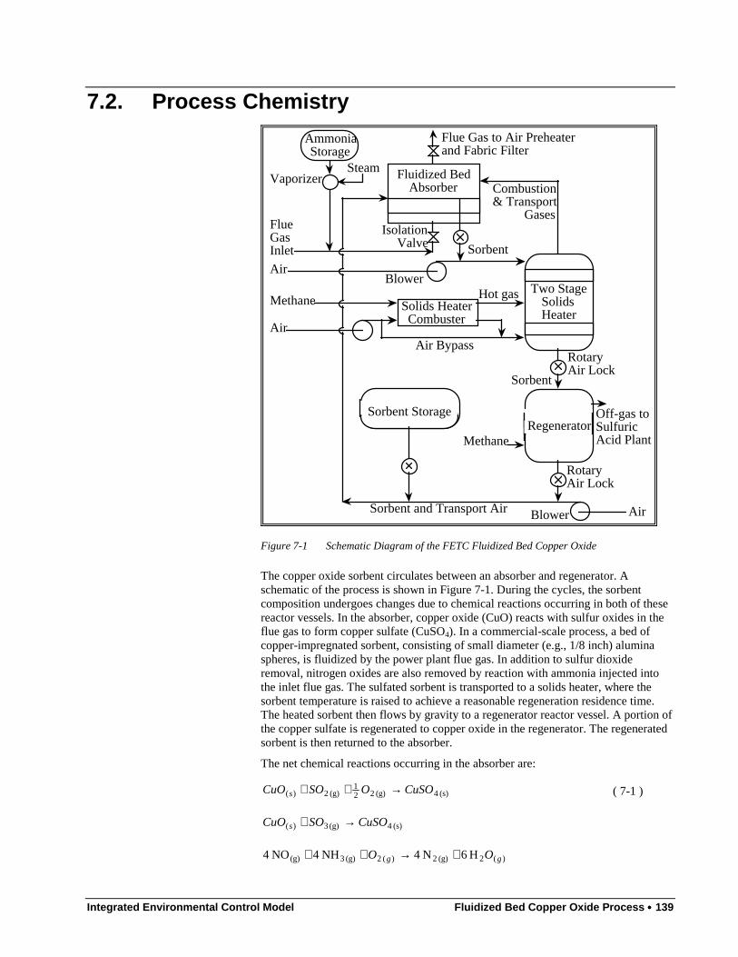
Integrated Environmental Control Model Fluidized Bed Copper Oxide Process •••• 139
7.2. Process Chemistry
Fluidized Bed Absorber�����������������������������������������
�����������������������������������������
Flue Gas Inlet
Isolation Valve Sorbent
Flue Gas to Air Preheater and Fabric Filter
Air
Solids Heater Combuster
Air
Methane
Air Bypass
Hot gas
Air
Vaporizer
Blower
Blower
Sorbent and Transport Air
Combustion & Transport
Gases
Methane
Sorbent
Off-gas to Sulfuric Acid Plant
Rotary Air Lock
������������������������������������������������������������������������������������������������������������������������
������������������������������������������������������������������������������������������������������������������������Regenerator
������������������������������������������������������������
Two Stage Solids Heater������������������������������
������������������������������
Rotary Air Lock
Ammonia Storage
Steam
���������������������������������������������������������������������������������������������������������������������������������
��������������������������������������������������������������������������������������Sorbent Storage
Figure 7-1 Schematic Diagram of the FETC Fluidized Bed Copper Oxide
The copper oxide sorbent circulates between an absorber and regenerator. Aschematic of the process is shown in Figure 7-1. During the cycles, the sorbentcomposition undergoes changes due to chemical reactions occurring in both of thesereactor vessels. In the absorber, copper oxide (CuO) reacts with sulfur oxides in theflue gas to form copper sulfate (CuSO4). In a commercial-scale process, a bed ofcopper-impregnated sorbent, consisting of small diameter (e.g., 1/8 inch) aluminaspheres, is fluidized by the power plant flue gas. In addition to sulfur dioxideremoval, nitrogen oxides are also removed by reaction with ammonia injected intothe inlet flue gas. The sulfated sorbent is transported to a solids heater, where thesorbent temperature is raised to achieve a reasonable regeneration residence time.The heated sorbent then flows by gravity to a regenerator reactor vessel. A portion ofthe copper sulfate is regenerated to copper oxide in the regenerator. The regeneratedsorbent is then returned to the absorber.
The net chemical reactions occurring in the absorber are:
(s) 4(g) 221
(g) 2)( CuSOOSOCuO s →++ ( 7-1 )
(s) 4(g) 3)( CuSOSOCuO s →+
)(2(g) 2)( 2(g) 3(g) H 6N 4NH 4NO 4 gg OO +→++
140 •••• Fluidized Bed Copper Oxide Process Integrated Environmental Control Model
)(2(g) 2)( 2(g) 3(g) 2 H 6N 3NH 4NO 2 gg OO +→++
During sorbent regeneration, an offgas containing sulfur dioxide (SO2) is evolved. Inthe regenerator, the sorbent flows downward in a moving bed, countercurrent to theregeneration off-gases. Copper oxide contained in the sorbent entering theregenerator may react rapidly with SO2 in the exiting off-gas to form copper sulfite(CuSO3) (Harriott and Markussen, 1992):
(s) 3(g) 2)( CuSOSOCuO s →+ ( 7-2 )
Thus, just inside the regenerator, the sorbent may consist of copper oxide, coppersulfite and copper sulfate. Some tests have also indicated the presence of compoundssuch as Cu2O and Cu2SO3 within the regenerator (Harriott and Markussen, 1992).However, pending further studies to provide a design basis, these species areexcluded from consideration in this model.
It is assumed that copper sulfite, copper sulfate, and copper oxide are regenerated tocopper with efficiencies ηr1, ηr2, and ηr3, respectively. The regeneration reactions
are:
)(2(g) 221
(g) 2)((g) 421
(s) 4 gs OHCOSOCuCHCuSO +++→+ ( 7-3 )
)(221
(g) 241
(g) 2)((g) 441
(s) 3 gs OHCOSOCuCHCuSO +++→+ ( 7-4 )
)(221
(g) 241
)((g) 441
(s) gs OHCOCuCHCuO ++→+ ( 7-5 )
The regenerated copper is rapidly oxidized to copper oxide upon contact withoxygen in solids transport air or the flue gas:
)((g) 221
)( ss CuOOCu →+
Similarly, any unregenerated copper sulfite is also assumed to completely oxidize tocopper sulfate upon contact with oxygen:
)( 4(g) 221
)( 3 ss CuSOOCuSO →+
Thus, the sorbent entering the absorber is assumed to contain only copper oxide andcopper sulfate.
The regeneration offgas is sent to a byproduct recovery plant. Here, it is assumedthat elemental sulfur is recovered in a Claus plant. The Claus reaction is:
)(2(l)(g) 2)(2 H 2S 3H 2 gg OSOS +→+
However, because the regeneration offgas contains no hydrogen sulfide, a portion ofthe SO2 must be reduced with natural gas to produce the required quantity ofhydrogen sulfide.
)(2(g) 2)(2)((g) 2(g) 4 H 2CO 2H 2SO 3CH 2 ggl OSS +++→+
Thus, some elemental sulfur is obtained via the reducing reaction, while theremainder is obtained via the Claus reaction. The overall reaction is:
)( 2)(2(l)(g) 2(g) 4 H 2S 2SO 2 gg COOCH ++→+
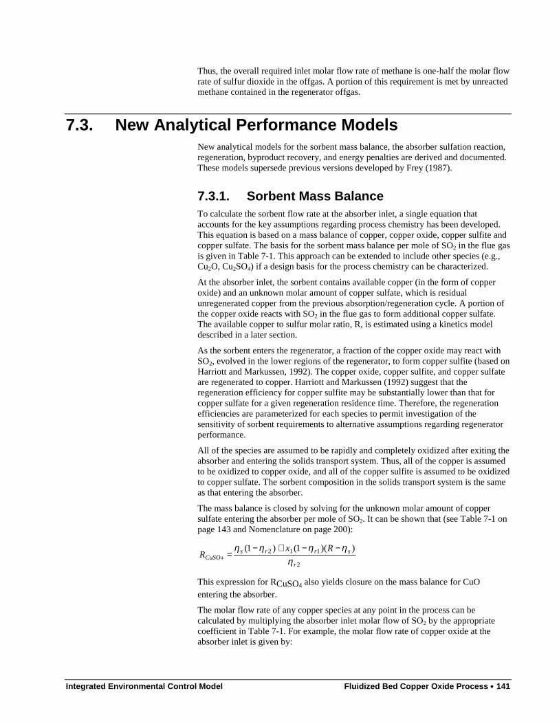
Integrated Environmental Control Model Fluidized Bed Copper Oxide Process •••• 141
Thus, the overall required inlet molar flow rate of methane is one-half the molar flowrate of sulfur dioxide in the offgas. A portion of this requirement is met by unreactedmethane contained in the regenerator offgas.
7.3. New Analytical Performance ModelsNew analytical models for the sorbent mass balance, the absorber sulfation reaction,regeneration, byproduct recovery, and energy penalties are derived and documented.These models supersede previous versions developed by Frey (1987).
7.3.1. Sorbent Mass BalanceTo calculate the sorbent flow rate at the absorber inlet, a single equation thataccounts for the key assumptions regarding process chemistry has been developed.This equation is based on a mass balance of copper, copper oxide, copper sulfite andcopper sulfate. The basis for the sorbent mass balance per mole of SO2 in the flue gasis given in Table 7-1. This approach can be extended to include other species (e.g.,Cu2O, Cu2SO4) if a design basis for the process chemistry can be characterized.
At the absorber inlet, the sorbent contains available copper (in the form of copperoxide) and an unknown molar amount of copper sulfate, which is residualunregenerated copper from the previous absorption/regeneration cycle. A portion ofthe copper oxide reacts with SO2 in the flue gas to form additional copper sulfate.The available copper to sulfur molar ratio, R, is estimated using a kinetics modeldescribed in a later section.
As the sorbent enters the regenerator, a fraction of the copper oxide may react withSO2, evolved in the lower regions of the regenerator, to form copper sulfite (based onHarriott and Markussen, 1992). The copper oxide, copper sulfite, and copper sulfateare regenerated to copper. Harriott and Markussen (1992) suggest that theregeneration efficiency for copper sulfite may be substantially lower than that forcopper sulfate for a given regeneration residence time. Therefore, the regenerationefficiencies are parameterized for each species to permit investigation of thesensitivity of sorbent requirements to alternative assumptions regarding regeneratorperformance.
All of the species are assumed to be rapidly and completely oxidized after exiting theabsorber and entering the solids transport system. Thus, all of the copper is assumedto be oxidized to copper oxide, and all of the copper sulfite is assumed to be oxidizedto copper sulfate. The sorbent composition in the solids transport system is the sameas that entering the absorber.
The mass balance is closed by solving for the unknown molar amount of coppersulfate entering the absorber per mole of SO2. It can be shown that (see Table 7-1 onpage 143 and Nomenclature on page 200):
2
112 ))(1()1(4
r
srrsCuSO
RxR
ηηηηη −−+−
=
This expression for RCuSO4 also yields closure on the mass balance for CuOentering the absorber.
The molar flow rate of any copper species at any point in the process can becalculated by multiplying the absorber inlet molar flow of SO2 by the appropriatecoefficient in Table 7-1. For example, the molar flow rate of copper oxide at theabsorber inlet is given by:

142 •••• Fluidized Bed Copper Oxide Process Integrated Environmental Control Model
iASOiACuO xMRM ,,, ,⋅= ( 7-6 )
where:
iASOiASOiASO MMM ,,,,,, 324 +=
The sorbent copper sulfate loading at the absorber entrance is given by:
iASOCuSOiACuSO xMRM ,,,, 44 ⋅= ( 7-7 )
Note that the total molar amount of copper entering the absorber is greater than theavailable molar amount. The available copper to sulfur molar ratio is defined as R,and the total copper to sulfur molar ratio is given by:
4CuSOtot RRR +=
A general formula is developed for calculating the sorbent mass flow as a function ofthe sorbent composition. Consider fresh sorbent, which contains copper only ascopper oxide. The convention used in previous studies has been to define the sorbentcomposition based on the weight percent of copper, assuming that all of the copper isin the form of copper oxide. Therefore, the sorbent mass flow rate on an equivalentfresh sorbent basis is given by:
)( 43, CuSOCuSOCuOCuCu
Cufreshs MMMM
W
MWm +++
=
However, in general, the sorbent may consist of other copper species as well. Whilethe total molar amount of copper is not affected by the speciation, the mass flow is.Thus, factors must be included to account for the effect of different copper specieson the sorbent mass flow rate. For example, for each mole of copper sulfate presentin the sorbent, there is an incremental increase in sorbent mass flow rate due to themass differential between a mole of copper oxide and a mole of copper sulfate. Thisdifference must be calculated on a copper basis:
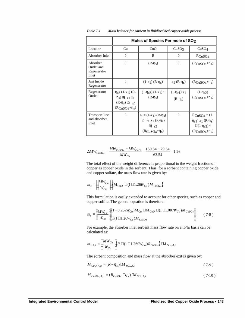
Integrated Environmental Control Model Fluidized Bed Copper Oxide Process •••• 143
Table 7-1 Mass balance for sorbent in fluidized bed copper oxide process
Moles of Species Per mole of SO 2
Location Cu CuO CuSO3 CuSO4
Absorber Inlet 0 R 0 RCuSO4
AbsorberOutlet andRegeneratorInlet
0 (R-ηs) 0 (RCuSO4+ηs)
Just InsideRegenerator
0 (1-x1) (R-ηs) x1 (R-ηs) (RCuSO4+ηs)
RegeneratorOutlet
ηr3 (1-x1) (R-
ηs) + ηr1 x1(R-ηs) + ηr2
(RCuSO4+ηs)
(1-ηr3) (1-x1) •
(R-ηs)
(1-ηr1) x1
(R-ηs)
(1-ηr2)
(RCuSO4+ηs)
Transport lineand absorberinlet
0 R = (1-x1) (R-ηs)
+ ηr1 x1 (R-ηs)
+ ηr2(RCuSO4+ηs)
0 RCuSO4 = (1-
ηr1) x1 (R-ηs)
+ (1-ηr2) •
(RCuSO4+ηs)
26.154.63
54.7954.15944 =−=
−=∆
Cu
CuOCuSOCuSO MW
MWMWMW
The total effect of the weight difference is proportional to the weight fraction ofcopper as copper oxide in the sorbent. Thus, for a sorbent containing copper oxideand copper sulfate, the mass flow rate is given by:
{ }4)26.11(M CuO CuSOCuCu
Cus MW
W
MWm ++
=
This formulation is easily extended to account for other species, such as copper andcopper sulfite. The general equation is therefore:
++
+++−=
4
3
)26.11(
)007.11()252.01(
CuSOCu
CuSOCuCuOCuCu
Cu
Cus
MW
MWMMW
W
MWm ( 7-8 )
For example, the absorber inlet sorbent mass flow rate on a lb/hr basis can becalculated as:
{ } iASOCuSOCuCu
CuiAs xMRWR
W
MWm ,,,, 4)260.11( ⋅++
=
The sorbent composition and mass flow at the absorber exit is given by:
iASOsoACuO xMRM ,,,, )( ⋅−= η ( 7-9 )
iASOsCuSOoACuSO xMRM ,,,, )( 44 ⋅+= η ( 7-10 )
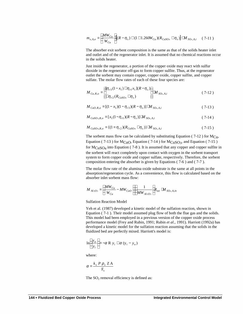
144 •••• Fluidized Bed Copper Oxide Process Integrated Environmental Control Model
{ } iASOsCuSOCusCu
CuoAs xMRWR
W
MWm ,,,, ))(260.11()( 4 ⋅+++−
= ηη ( 7-11 )
The absorber exit sorbent composition is the same as that of the solids heater inletand outlet and of the regenerator inlet. It is assumed that no chemical reactions occurin the solids heater.
Just inside the regenerator, a portion of the copper oxide may react with sulfurdioxide in the regenerator off-gas to form copper sulfite. Thus, at the regeneratoroutlet the sorbent may contain copper, copper oxide, copper sulfite, and coppersulfate. The molar flow rates of each of these four species are:
iASO
sCuSOr
srr
oRCu xMR
RxxM ,,
2
1113
,,)(
)]()1([
4
⋅
++
−+−=
ηη
ηηη( 7-12 )
iASOsroRCuO xMRxM ,,31,, )])(1)(1[( ⋅−−−= ηη ( 7-13 )
iASOsroRCuSO xMRxM ,,11,, )])(1([3 ⋅−−= ηη ( 7-14 )
iASOsCuSOroRCuSO xMRM ,,2,, )})(1{( 44 ⋅+== ηη ( 7-15 )
The sorbent mass flow can be calculated by substituting Equation ( 7-12 ) for MCu,Equation ( 7-13 ) for MCuO, Equation ( 7-14 ) for MCuSO3, and Equation ( 7-15 )
for MCuSO4 into Equation ( 7-8 ). It is assumed that any copper and copper sulfite in
the sorbent will react completely upon contact with oxygen in the sorbent transportsystem to form copper oxide and copper sulfate, respectively. Therefore, the sorbentcomposition entering the absorber is given by Equations ( 7-6 ) and ( 7-7 ).
The molar flow rate of the alumina oxide substrate is the same at all points in theabsorption/regeneration cycle. As a convenience, this flow is calculated based on theabsorber inlet sorbent mass flow:
inASOtotOAl
CuOCu
CuOAl xMR
MWMW
W
MWM ,,
32
32
1 ⋅
−=
Sulfation Reaction Model
Yeh et al. (1987) developed a kinetic model of the sulfation reaction, shown inEquation ( 7-1 ). Their model assumed plug flow of both the flue gas and the solids.This model had been employed in a previous version of the copper oxide processperformance model (Frey and Rubin, 1991; Rubin et al., 1991). Harriott (1992a) hasdeveloped a kinetic model for the sulfation reaction assuming that the solids in thefluidized bed are perfectly mixed. Harriott's model is:
)(y R ln i oii
o yyy
y−+−=
αα
where:
sF
A Z ss Pk ρα =
The SO2 removal efficiency is defined as:
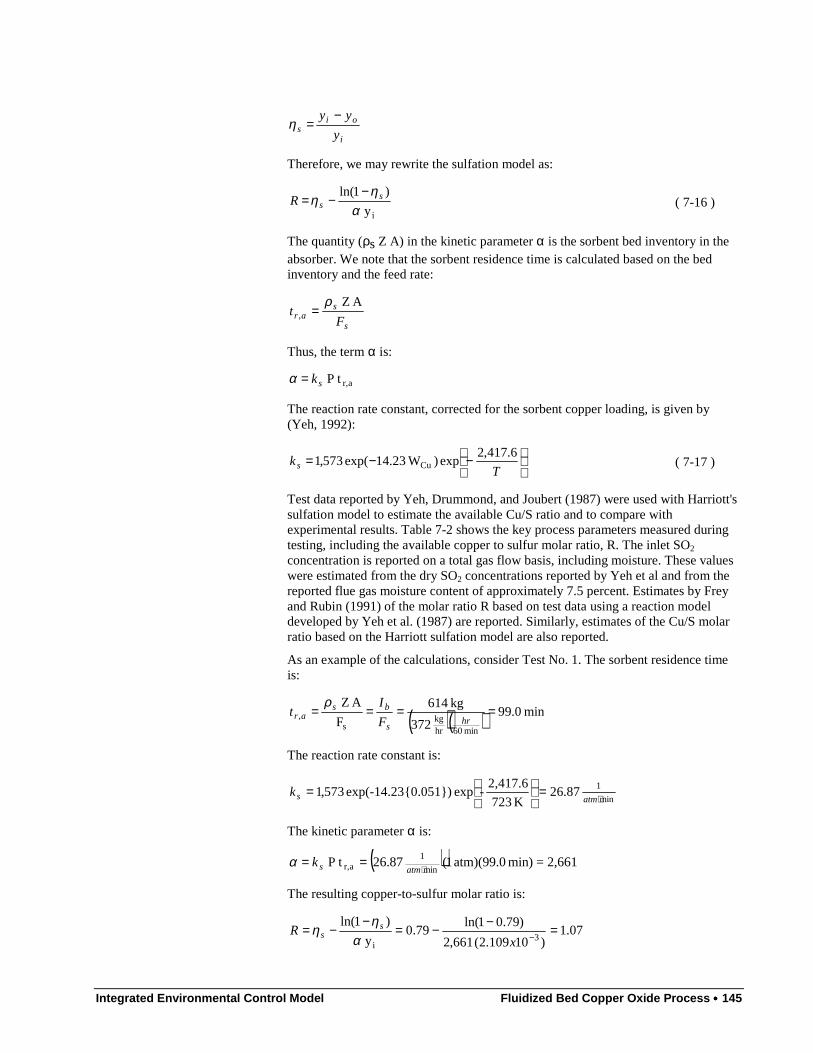
Integrated Environmental Control Model Fluidized Bed Copper Oxide Process •••• 145
i
ois y
yy −=η
Therefore, we may rewrite the sulfation model as:
iy
)1ln(
αη
η ssR
−−= ( 7-16 )
The quantity (ρs Z A) in the kinetic parameter α is the sorbent bed inventory in theabsorber. We note that the sorbent residence time is calculated based on the bedinventory and the feed rate:
s
sar F
tA Z
,ρ
=
Thus, the term α is:
ar, tP sk=α
The reaction rate constant, corrected for the sorbent copper loading, is given by(Yeh, 1992):
−−=
Tks
6.417,2exp) W23.14exp( 573,1 Cu ( 7-17 )
Test data reported by Yeh, Drummond, and Joubert (1987) were used with Harriott'ssulfation model to estimate the available Cu/S ratio and to compare withexperimental results. Table 7-2 shows the key process parameters measured duringtesting, including the available copper to sulfur molar ratio, R. The inlet SO2
concentration is reported on a total gas flow basis, including moisture. These valueswere estimated from the dry SO2 concentrations reported by Yeh et al and from thereported flue gas moisture content of approximately 7.5 percent. Estimates by Freyand Rubin (1991) of the molar ratio R based on test data using a reaction modeldeveloped by Yeh et al. (1987) are reported. Similarly, estimates of the Cu/S molarratio based on the Harriott sulfation model are also reported.
As an example of the calculations, consider Test No. 1. The sorbent residence timeis:
( )( ) min 0.99372
kg 614
F
A Z
min 60hrkg
s, ====
hrs
bsar F
It
ρ
The reaction rate constant is:
min
187.26K 723
2,417.6-exp {0.051}) exp(-14.23 573,1
⋅=
=
atmsk
The kinetic parameter α is:
( ) 2,661=min) atm)(99.0 1(87.26 tP min
1ar, ⋅
==atmskα
The resulting copper-to-sulfur molar ratio is:
07.1)10109.2( 661,2
)79.01ln(79.0
y
)1ln(3
i
=−−=−
−= −xR s
s αη
η

146 •••• Fluidized Bed Copper Oxide Process Integrated Environmental Control Model
Figure 7-2 shows a comparison of the Cu/S ratio estimated using the FETC modelversus experimental results. Figure 7-3 shows a similar comparison using theHarriott model.
The comparison of the Harriott and FETC sulfation models with experimental dataindicates that Harriott's model provides generally better estimates of the Cu/S ratiothan the FETC model. Although both models yield estimates typically within ± 10percent of the experimentally measured values, the estimates from Harriott's modeltend to be less scattered from the parity line. Harriott's model appears to besomewhat conservative in predicting Cu/S ratios slightly higher than theexperimentally measured results. The model results diverge most noticeable for thehigh Cu/S ratios, which represents testing with low (18-inch) fluidized bed heights.Such bed heights are unlikely for commercial scale designs, and the experimentalresults themselves are considered less certain than the ones reported for higher bedheights. Therefore, Harriott's model is employed here.
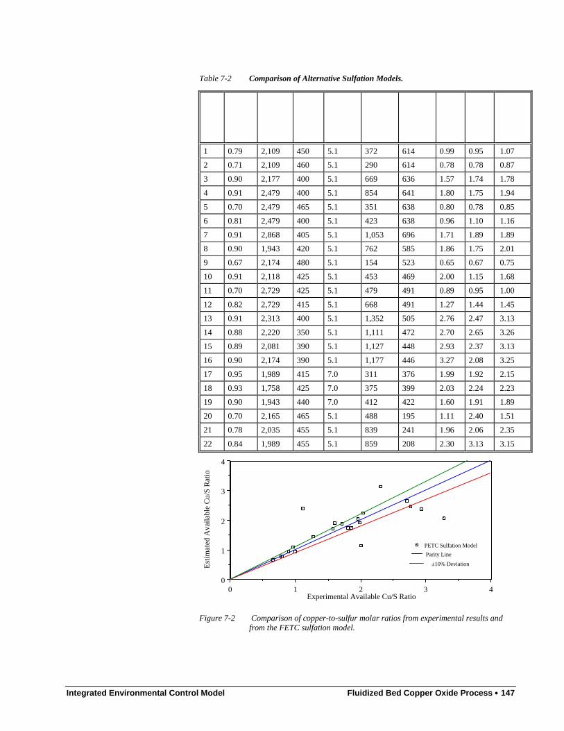
Integrated Environmental Control Model Fluidized Bed Copper Oxide Process •••• 147
Table 7-2 Comparison of Alternative Sulfation Models.
� � � �� � �
� � �� � � � �� � � � � � �
� � � � �� � �
� � � � �� � � �
� � �� � � � �� � � �
� �� � � � � � �� � � � � �
� � � � � � �� � � �� � � � � �
� � �� � � � � � ��
� � � �
� � � � � �� � � �� � � � �
� � � �� � � � �� � � �
� � � � � � � �� � � � �� � � �
1 0.79 2,109 450 5.1 372 614 0.99 0.95 1.07
2 0.71 2,109 460 5.1 290 614 0.78 0.78 0.87
3 0.90 2,177 400 5.1 669 636 1.57 1.74 1.78
4 0.91 2,479 400 5.1 854 641 1.80 1.75 1.94
5 0.70 2,479 465 5.1 351 638 0.80 0.78 0.85
6 0.81 2,479 400 5.1 423 638 0.96 1.10 1.16
7 0.91 2,868 405 5.1 1,053 696 1.71 1.89 1.89
8 0.90 1,943 420 5.1 762 585 1.86 1.75 2.01
9 0.67 2,174 480 5.1 154 523 0.65 0.67 0.75
10 0.91 2,118 425 5.1 453 469 2.00 1.15 1.68
11 0.70 2,729 425 5.1 479 491 0.89 0.95 1.00
12 0.82 2,729 415 5.1 668 491 1.27 1.44 1.45
13 0.91 2,313 400 5.1 1,352 505 2.76 2.47 3.13
14 0.88 2,220 350 5.1 1,111 472 2.70 2.65 3.26
15 0.89 2,081 390 5.1 1,127 448 2.93 2.37 3.13
16 0.90 2,174 390 5.1 1,177 446 3.27 2.08 3.25
17 0.95 1,989 415 7.0 311 376 1.99 1.92 2.15
18 0.93 1,758 425 7.0 375 399 2.03 2.24 2.23
19 0.90 1,943 440 7.0 412 422 1.60 1.91 1.89
20 0.70 2,165 465 5.1 488 195 1.11 2.40 1.51
21 0.78 2,035 455 5.1 839 241 1.96 2.06 2.35
22 0.84 1,989 455 5.1 859 208 2.30 3.13 3.15
432100
1
2
3
4
PETC Sulfation Model
Parity Line
Experimental Available Cu/S Ratio
Est
imat
ed A
vaila
ble
Cu/
S R
atio
±10% Deviation
Figure 7-2 Comparison of copper-to-sulfur molar ratios from experimental results andfrom the FETC sulfation model.
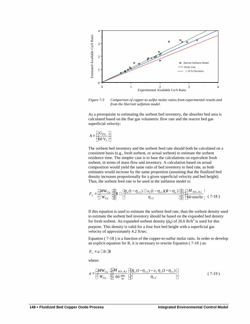
148 •••• Fluidized Bed Copper Oxide Process Integrated Environmental Control Model
432100
1
2
3
4
Harriott Sulfation Model
Parity Line
Experimental Available Cu/S RatioE
stim
ated
Ava
ilabl
e C
u/S
Rat
io
± 10 % Deviation
Figure 7-3 Comparison of copper-to-sulfur molar ratios from experimental results andfrom the Harriott sulfation model.
As a prerequisite to estimating the sorbent bed inventory, the absorber bed area iscalculated based on the flue gas volumetric flow rate and the reactor bed gassuperficial velocity:
=
sV 60FGG
A
The sorbent bed inventory and the sorbent feed rate should both be calculated on aconsistent basis (e.g., fresh sorbent, or actual sorbent) to estimate the sorbentresidence time. The simpler case is to base the calculations on equivalent freshsorbent, in terms of mass flow and inventory. A calculation based on actualcomposition would yield the same ratio of bed inventory to feed rate, as bothestimates would increase by the same proportion (assuming that the fluidized beddensity increases proportionally for a given superficial velocity and bed height).Thus, the sorbent feed rate to be used in the sulfation model is:
⋅
−−+−+
=
min/hr 60
))(1()1( ,,
2
112 iASO
r
srrs
Cu
Cus
xMRxR
W
MWF
ηηηηη
( 7-18 )
If this equation is used to estimate the sorbent feed rate, than the sorbent density usedto estimate the sorbent bed inventory should be based on the expanded bed densityfor fresh sorbent. An expanded sorbent density (ρs) of 26.6 lb/ft3 is used for thispurpose. This density is valid for a four foot bed height with a superficial gasvelocity of approximately 4.2 ft/sec.
Equation ( 7-18 ) is a function of the copper-to-sulfur molar ratio. In order to developan explicit equation for R, it is necessary to rewrite Equation ( 7-18 ) as:
RbaFs ⋅+=
where:
−−−
=
2
112min
,, )1( )1(
60 r
rsrs
hr
iASO
Cu
Cu xM
W
MWa
x
ηηηηη
( 7-19 )
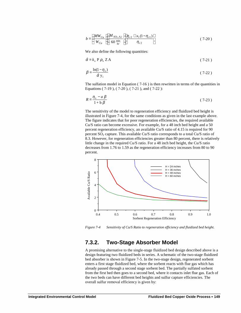
Integrated Environmental Control Model Fluidized Bed Copper Oxide Process •••• 149
−+
=
2
112min
,, )1(
60 r
rr
hr
iASO
Cu
Cu xM
W
MWb
x
ηηη
( 7-20 )
We also define the following quantities:
A Z P ˆ sρα sk= ( 7-21 )
iy ˆ
)1ln(
αη
β s−= ( 7-22 )
The sulfation model in Equation ( 7-16 ) is then rewritten in terms of the quantities inEquations ( 7-19 ), ( 7-20 ), ( 7-21 ), and ( 7-22 ):
ββη
b+1
aR s −
= ( 7-23 )
The sensitivity of the model to regeneration efficiency and fluidized bed height isillustrated in Figure 7-4, for the same conditions as given in the last example above.The figure indicates that for poor regeneration efficiencies, the required availableCu/S ratio can become excessive. For example, for a 48 inch bed height and a 50percent regeneration efficiency, an available Cu/S ratio of 4.15 is required for 90percent SO2 capture. This available Cu/S ratio corresponds to a total Cu/S ratio of8.3. However, for regeneration efficiencies greater than 80 percent, there is relativelylittle change in the required Cu/S ratio. For a 48 inch bed height, the Cu/S ratiodecreases from 1.76 to 1.59 as the regeneration efficiency increases from 80 to 90percent.
1.00.90.80.70.60.50.40
2
4
6
8
H = 24 inchesH = 36 inchesH = 48 inchesH = 60 inches
Sorbent Regeneration Efficiency
Ava
ilabl
e C
u/S
Rat
io
Figure 7-4 Sensitivity of Cu/S Ratio to regeneration efficiency and fluidized bed height.
7.3.2. Two-Stage Absorber ModelA promising alternative to the single-stage fluidized bed design described above is adesign featuring two fluidized beds in series. A schematic of the two-stage fluidizedbed absorber is shown in Figure 7-5. In the two-stage design, regenerated sorbententers a first stage fluidized bed, where the sorbent reacts with flue gas which hasalready passed through a second stage sorbent bed. The partially sulfated sorbentfrom the first bed then goes to a second bed, where it contacts inlet flue gas. Each ofthe two beds can have different bed heights and sulfur capture efficiencies. Theoverall sulfur removal efficiency is given by:
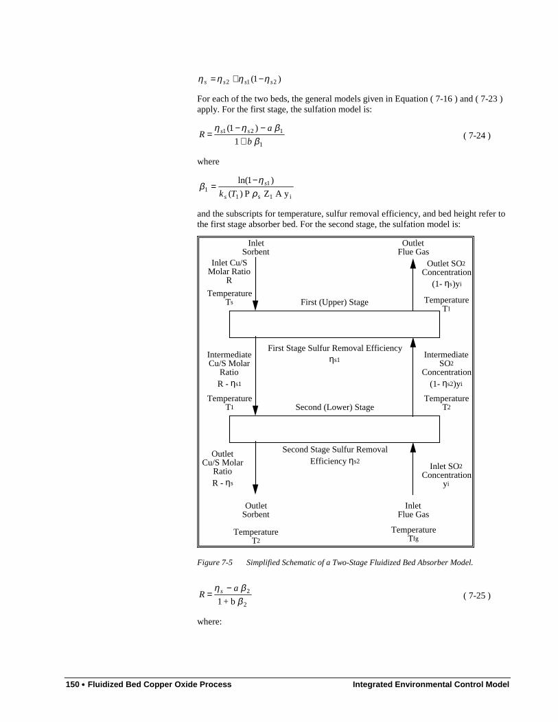
150 •••• Fluidized Bed Copper Oxide Process Integrated Environmental Control Model
)1( 212 ssss ηηηη −+=
For each of the two beds, the general models given in Equation ( 7-16 ) and ( 7-23 )apply. For the first stage, the sulfation model is:
1
121
1
)1(
ββηη
b
aR ss
+−−
= ( 7-24 )
where
i1s1
11 yA Z P )(
)1ln(
ρη
βTks
s−=
and the subscripts for temperature, sulfur removal efficiency, and bed height refer tothe first stage absorber bed. For the second stage, the sulfation model is:
����������������������������������������������������������������������������������������������������������������������������������������������������������������������������������������������������������������������������������������������������������������������������������������������������������������������������������������������������������������������������������������������������������������������������������������������������������������������������������������������������
����������������������������������������������������������������������������������������������������������������������������������������������������������������������������������������������������������������������������������������������������������������������������������������������������������������������������������������������������������������������������������������������������������������������������������������������������������������������������������������������������
First (Upper) Stage
Second (Lower) Stage
Inlet Sorbent
Outlet Flue Gas
Outlet Sorbent
Inlet Flue Gas
Inlet Cu/S Molar Ratio
R
Intermediate Cu/S Molar
Ratio R - ηs1
Outlet Cu/S Molar
Ratio R - ηs
Inlet SO2 Concentration
yi
Intermediate SO2
Concentration (1- ηs2)yi
Outlet SO2 Concentration
(1- ηs)yi
First Stage Sulfur Removal Efficiency ηs1
Second Stage Sulfur Removal Efficiency ηs2
Temperature T2
Temperature Tfg
Temperature T2
Temperature T1
Temperature T1
Temperature Ts
Figure 7-5 Simplified Schematic of a Two-Stage Fluidized Bed Absorber Model.
2
2
b+1
ββη a
R s −= ( 7-25 )
where:
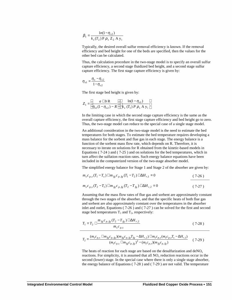
Integrated Environmental Control Model Fluidized Bed Copper Oxide Process •••• 151
i2s2
21 yA Z P )(
)1(1
ρη
βTk
n
s
s−=
Typically, the desired overall sulfur removal efficiency is known. If the removalefficiency and bed height for one of the beds are specified, then the values for theother bed can be calculated.
Thus, the calculation procedure in the two-stage model is to specify an overall sulfurcapture efficiency, a second stage fluidized bed height, and a second stage sulfurcapture efficiency. The first stage capture efficiency is given by:
2
21 1 s
sss η
ηηη
−−
=
The first stage bed height is given by:
−
−−
+=is1
1
2s11 yA )(
)1ln(
)1(
R
ρη
ηη PTkR
baZ
s
s
s
In the limiting case in which the second stage capture efficiency is the same as theoverall capture efficiency, the first stage capture efficiency and bed height go to zero.Thus, the two-stage model can reduce to the special case of a single stage model.
An additional consideration in the two-stage model is the need to estimate the bedtemperatures for both stages. To estimate the bed temperature requires developing amass balance for the sorbent and flue gas in each stage. The energy balance is afunction of the sorbent mass flow rate, which depends on R. Therefore, it isnecessary to iterate on solutions for R obtained from the kinetic-based models inEquations ( 7-24 ) and ( 7-25 ) and on solutions for the bed temperatures, which inturn affect the sulfation reaction rates. Such energy balance equations have beenincluded in the computerized version of the two-stage absorber model.
The simplified energy balance for Stage 1 and Stage 2 of the absorber are given by:
0)()( 1,21,1, =∆+−+− rfgpfgssps HTTcmTTcm ( 7-26 )
0)()( 2,2,12, =∆+−+− rfgfgpfgsps HTTcmTTcm ( 7-27 )
Assuming that the mass flow rates of flue gas and sorbent are approximately constantthrough the two stages of the absorber, and that the specific heats of both flue gasand sorbent are also approximately constant over the temperatures in the absorberinlet and outlet, Equations ( 7-26 ) and ( 7-27 ) can be solved for the first and secondstage bed temperatures T1 and T2, respectively:
sps
rfgfgpfg
cm
HTTcmTT
,
2,2,21
)( ∆+−+= ( 7-28 )
))(()(
)()()(
,,2
,,
1,,,2,,,,2
fgpfgspsfgpfgsps
rsspsspsrfgfgpfgfgpfgsps
cmcmcmcm
HTcmcmHTcmcmcmT
−+∆−+∆−+
= ( 7-29 )
The heats of reaction for each stage are based on the desulfurization and deNOx
reactions. For simplicity, it is assumed that all NOx reduction reactions occur in thesecond (lower) stage. In the special case where there is only a single stage absorber,the energy balance of Equations ( 7-28 ) and ( 7-29 ) are not valid. The temperature
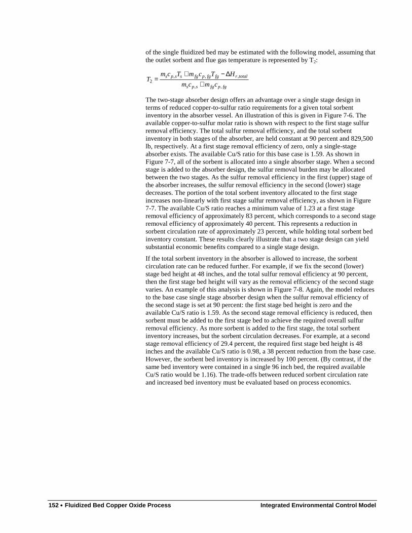
152 •••• Fluidized Bed Copper Oxide Process Integrated Environmental Control Model
of the single fluidized bed may be estimated with the following model, assuming thatthe outlet sorbent and flue gas temperature is represented by T2:
fgpfgsps
totalrfgfgpfgssps
cmcm
HTcmTcmT
,,
,,,2 +
∆−+=
The two-stage absorber design offers an advantage over a single stage design interms of reduced copper-to-sulfur ratio requirements for a given total sorbentinventory in the absorber vessel. An illustration of this is given in Figure 7-6. Theavailable copper-to-sulfur molar ratio is shown with respect to the first stage sulfurremoval efficiency. The total sulfur removal efficiency, and the total sorbentinventory in both stages of the absorber, are held constant at 90 percent and 829,500lb, respectively. At a first stage removal efficiency of zero, only a single-stageabsorber exists. The available Cu/S ratio for this base case is 1.59. As shown inFigure 7-7, all of the sorbent is allocated into a single absorber stage. When a secondstage is added to the absorber design, the sulfur removal burden may be allocatedbetween the two stages. As the sulfur removal efficiency in the first (upper) stage ofthe absorber increases, the sulfur removal efficiency in the second (lower) stagedecreases. The portion of the total sorbent inventory allocated to the first stageincreases non-linearly with first stage sulfur removal efficiency, as shown in Figure7-7. The available Cu/S ratio reaches a minimum value of 1.23 at a first stageremoval efficiency of approximately 83 percent, which corresponds to a second stageremoval efficiency of approximately 40 percent. This represents a reduction insorbent circulation rate of approximately 23 percent, while holding total sorbent bedinventory constant. These results clearly illustrate that a two stage design can yieldsubstantial economic benefits compared to a single stage design.
If the total sorbent inventory in the absorber is allowed to increase, the sorbentcirculation rate can be reduced further. For example, if we fix the second (lower)stage bed height at 48 inches, and the total sulfur removal efficiency at 90 percent,then the first stage bed height will vary as the removal efficiency of the second stagevaries. An example of this analysis is shown in Figure 7-8. Again, the model reducesto the base case single stage absorber design when the sulfur removal efficiency ofthe second stage is set at 90 percent: the first stage bed height is zero and theavailable Cu/S ratio is 1.59. As the second stage removal efficiency is reduced, thensorbent must be added to the first stage bed to achieve the required overall sulfurremoval efficiency. As more sorbent is added to the first stage, the total sorbentinventory increases, but the sorbent circulation decreases. For example, at a secondstage removal efficiency of 29.4 percent, the required first stage bed height is 48inches and the available Cu/S ratio is 0.98, a 38 percent reduction from the base case.However, the sorbent bed inventory is increased by 100 percent. (By contrast, if thesame bed inventory were contained in a single 96 inch bed, the required availableCu/S ratio would be 1.16). The trade-offs between reduced sorbent circulation rateand increased bed inventory must be evaluated based on process economics.
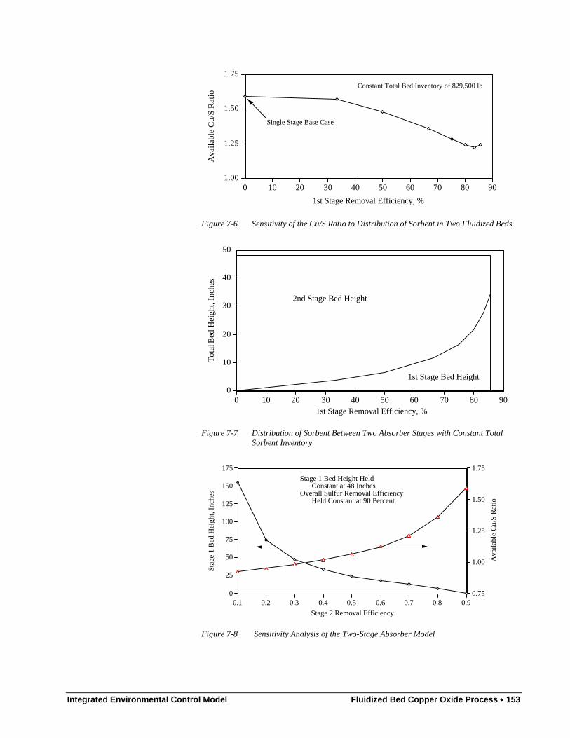
Integrated Environmental Control Model Fluidized Bed Copper Oxide Process •••• 153
1.00
1.25
1.50
1.75
Ava
ilabl
e C
u/S
Rat
io
0 10 20 30 40 50 60 70 80 90
1st Stage Removal Efficiency, %
Constant Total Bed Inventory of 829,500 lb
Single Stage Base Case
Figure 7-6 Sensitivity of the Cu/S Ratio to Distribution of Sorbent in Two Fluidized Beds
��������������������������������������������������������������������������������������������������������������������������������������������������������������������������������������������������������������������������������������������������������������������������������������������������������������������������������������������������������������������������������������������������������������������������������������������������������������������������������������������������������������������������������������������������������������������������������������������������������������������������������������������������������������������������������������������������������������������������������������������������������������������������������������������������������������������������������������������������������������������������������������������������������������������������������������������������������������������������������������������������������������������������������������������������������������������������������������������������������������������������������������������������������������������������������������������������������������������������������������������������������������������������������������������������������������������������������������������������������������������������������������������������������������������������������������������������������������������������������������
�����������������������������������������������������������������������������������������������������������������������������������������������������������������������������������������������������������������������������������������������������������������������������������������������������������������������������������������������������������������������������������������������������������������������������������������������������������������������������������������������������������������������������������������������������������������������������������������������������������������������������������������������������������������������������������������������������������������������������������������������������������������������������������������������������������������������������������������������������������������������������������������������������������������������������������������������������������������������������������������������������������������������������������������������������������������������������������������������������������������������������������������������������������������������������������������������������������������������������������������������������������������������������������������������������������������������������������������������������������������������������������������������������������������������������������������������������������������������������������������������������������������������������������������������������������������������������������������������������������������������������������������������������������������������������������������������������������������������������������������������������������������������������������������������������������������������������������������������������������������������������������������������������������������������������������
0
10
20
30
40
50
Tot
al B
ed H
eigh
t, I
nche
s
0 10 20 30 40 50 60 70 80 901st Stage Removal Efficiency, %
2nd Stage Bed Height
1st Stage Bed Height
Figure 7-7 Distribution of Sorbent Between Two Absorber Stages with Constant TotalSorbent Inventory
0.75
1.00
1.25
1.50
1.75
Ava
ilabl
e C
u/S
Rat
io
0
25
50
75
100
125
150
175
Sta
ge 1
Bed
Hei
ght,
Inch
es
0.1 0.2 0.3 0.4 0.5 0.6 0.7 0.8 0.9
Stage 2 Removal Efficiency
Stage 1 Bed Height Held Constant at 48 Inches
Overall Sulfur Removal Efficiency Held Constant at 90 Percent
Figure 7-8 Sensitivity Analysis of the Two-Stage Absorber Model
154 •••• Fluidized Bed Copper Oxide Process Integrated Environmental Control Model
7.3.3. Regeneration Performance ModelThe key chemical equations governing the performance of the regenerator are givenby Equations ( 7-2 ) to ( 7-5 ). The regenerator mass and energy balance for thecopper oxide model developed by Frey (1987) is revised here based on the need toaccount for the potential formation of copper sulfite in the regenerator (Harriott,1992c; Harriott and Markussen, 1992). Furthermore, a kinetic model developed byHarriott is used to estimate regenerator residence time associated with regenerationof copper sulfate.
7.3.3.1. Regenerator Mass BalanceThe mass balance for sorbent in the regenerator is given by Equations ( 7-9 ) to (7-15 ). At the regenerator inlet, the molar fraction of total copper in the sorbentwhich is in the form of copper sulfate is given by:
tot
sCuSOCuSO R
Rx
)( 44
η+=
The mass balance for gaseous species in the regenerator includes methane at theregenerator inlet, and regeneration off-gas containing methane, sulfur dioxide,carbon dioxide, and water vapor.
The total amount of methane required for regeneration is estimated per Harriott(1992c) based on the minimum requirement for 100 percent regeneration and amultiplier for excess methane. For each mole of copper sulfate, one-half mole ofmethane is required, and for each mole of copper oxide or copper sulfite, one-quartermole of methane is required, as indicated by equations ( 7-4 ) and ( 7-5 ). Thus, thetotal methane requirement is:
xSOtotCuSOCuSOCHiRCH MRxxRM ,, )]1(25.05.0[ 4444 −+=
The amount of sulfur dioxide produced depends on the fraction of copper oxideconverted to copper sulfite and the actual regeneration efficiencies for copper sulfiteand copper sulfate. Sulfur dioxide is consumed by the conversion of copper oxide tocopper sulfite, while it is produced by the regeneration of both copper sulfite andcopper sulfate. The net production of sulfur dioxide is given by:
x442 SOtot112,, M R )]1()1([ CuSOrCuSOroRSO xxxM −−+= ηη ( 7-30 )
Water vapor is produced in all three of the assumed regeneration reactions. Thus, thetotal amount of water vapor produced is:
{ }
x
442
SOtot
1311CuSO2,,
M R
)]1([)1(5.0
×
−+×−+×= xxxM rrCuSOroROH ηηη( 7-31 )
For each mole of water vapor produced, one-half mole of carbon dioxide is producedas shown in Equations ( 7-3 ), ( 7-4 ) and ( 7-5 ). Therefore, the total molar amountof carbon dioxide produced is:
oROHoRCOM ,,,, 22 M 5.0= ( 7-32 )
The molar amount of methane consumed in the regenerator is the same as the molaramount of carbon dioxide produced. Therefore, the net amount of methane exitingthe regenerator is given by:
oRCOiRCHoRCH MMM ,,,,,, 244 −=

Integrated Environmental Control Model Fluidized Bed Copper Oxide Process •••• 155
7.3.3.2. Regenerator Energy BalanceThe regenerator energy balance is calculated based on the sorbent and gas massbalance given above, and the energy released or absorbed by the chemical reactionsoccurring in the regenerator. A total of four chemical reactions are assumed to occurwithin the regenerator and each has an associated heat of reaction.
For the reaction of copper oxide to form copper sulfite (Equation ( 7-2 )), a heat ofreaction cannot be calculated based on heats of formation because thermodynamicdata for copper sulfite are not available in the standard reference literature (e.g.,Barin and Knacke, 1973; Barin, I., O. Knacke, and O. Kubaschewski, 1977; Chase etal., 1985). Harriott (1992c) estimated a heat of reaction based on data for SO2
oxidation and CuSO4 formation. The estimated heat of reaction is ∆H1 = -93,240Btu/lbmole CuO.
Heats of reaction for the regeneration of copper sulfate and copper oxide (Equations( 7-3 ) and ( 7-5 ), respectively) were estimated by Frey (1987) and are ∆H2 = 30,700Btu/lbmole CuSO4 and ∆H3 = -19,380 Btu/lbmole CuO, respectively. The heat ofreaction for the regeneration of copper sulfite was estimated based on the heats ofreaction for the regeneration of copper oxide and the conversion of copper oxide tocopper sulfite:
(s) (g)(s) CuSOSOCuO 32 →+ 240,931 −=∆H
Btu/lbmole CuO
(g) (g)
(g)(s) (g) (s)
OHCO
SOCuCHCuSO
22
243
21
41
41
++
+→+?4 =∆H
(g) (g)(s) (g)(s) OHCOCuCHCuO 224 21
41
41 ++→+ 413 HHH ∆+∆=∆
Thus:
4134 CuSO Btu/lbmole 680,73=∆−∆=∆ HHH
The total heat of reaction for all chemical reactions in the regenerator is given by:
411313
2211,
)1( )1)(1(
)1(
44
44
HxxHxx
HxHxxH
CuSOrCuSO
CuSOrCuSOtotr
∆−+∆−−+
∆+∆−=∆
ηη
η
The total molar flow of solids entering the regenerator is:
iROAliRCuSOiRCuSOiRCuOiRCuiRs MMMMMM ,,,,,,,,,,,, 3243 ++++=
The solids enter at a specified temperature TR,i, which is the same as the solids heateroutlet temperature. The enthalpy of the solids entering the regenerator is given by:
∑∑
=
==
3243
3243
,,,,,,
,,,,,,,
,
)(ˆ
)(ˆ
OAlCuSOCuSOCuOCujiRj
iRjOAlCuSOCuSOCuOCuj
iRj
iRsM
ThM
Th
The total molar flow and enthalpy of the solids at the regenerator outlet are similarlycalculated.
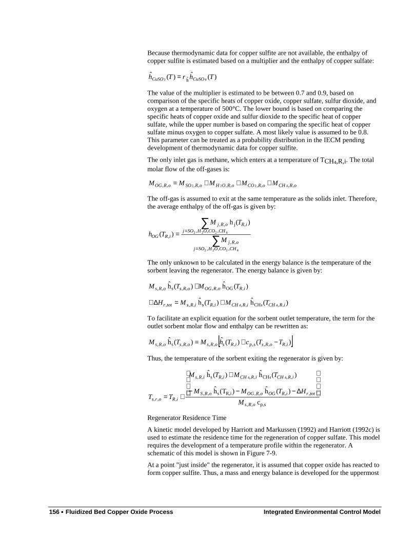
156 •••• Fluidized Bed Copper Oxide Process Integrated Environmental Control Model
Because thermodynamic data for copper sulfite are not available, the enthalpy ofcopper sulfite is estimated based on a multiplier and the enthalpy of copper sulfate:
)(ˆ)(ˆ43 h
ThrTh CuSOCuSO =
The value of the multiplier is estimated to be between 0.7 and 0.9, based oncomparison of the specific heats of copper oxide, copper sulfate, sulfur dioxide, andoxygen at a temperature of 500°C. The lower bound is based on comparing thespecific heats of copper oxide and sulfur dioxide to the specific heat of coppersulfate, while the upper number is based on comparing the specific heat of coppersulfate minus oxygen to copper sulfate. A most likely value is assumed to be 0.8.This parameter can be treated as a probability distribution in the IECM pendingdevelopment of thermodynamic data for copper sulfite.
The only inlet gas is methane, which enters at a temperature of TCH4,R,i. The totalmolar flow of the off-gases is:
oRCHoRCOoROHoRSOoROG MMMMM ,,,,,,,,,, 4222 +++=
The off-gas is assumed to exit at the same temperature as the solids inlet. Therefore,the average enthalpy of the off-gas is given by:
∑∑
=
==
4222
4222
,,,,,
,,,,j,,
,
)(h
)(
CHCOOHSOjoRj
CHCOOHSOjiRoRj
iROGM
TM
Th
The only unknown to be calculated in the energy balance is the temperature of thesorbent leaving the regenerator. The energy balance is given by:
)(h )(h
)(h )(h
,,CH,,,s,,,
,OG,,,,s,,
444 iRCHiRCHiRiRstotr
iRoROGoRsoRs
TMTMH
TMTM
+=∆+
+
To facilitate an explicit equation for the sorbent outlet temperature, the term for theoutlet sorbent molar flow and enthalpy can be rewritten as:
[ ])()(ˆ)(h ,,,,,,,,,s,, iRoRsspiRsoRsoRsoRs TTcThMTM −+=
Thus, the temperature of the sorbent exiting the regenerator is given by:
sp,,,
,,,,iR,s,,
,,CH,,,s,,
,,, c
)(h )(Th
)(h )(h 444
oRs
totriROGoROGoRS
iRCHiRCHiRiRs
iRors M
HTMM
TMTM
TT
∆−−−
+
+=
Regenerator Residence Time
A kinetic model developed by Harriott and Markussen (1992) and Harriott (1992c) isused to estimate the residence time for the regeneration of copper sulfate. This modelrequires the development of a temperature profile within the regenerator. Aschematic of this model is shown in Figure 7-9.
At a point "just inside" the regenerator, it is assumed that copper oxide has reacted toform copper sulfite. Thus, a mass and energy balance is developed for the uppermost
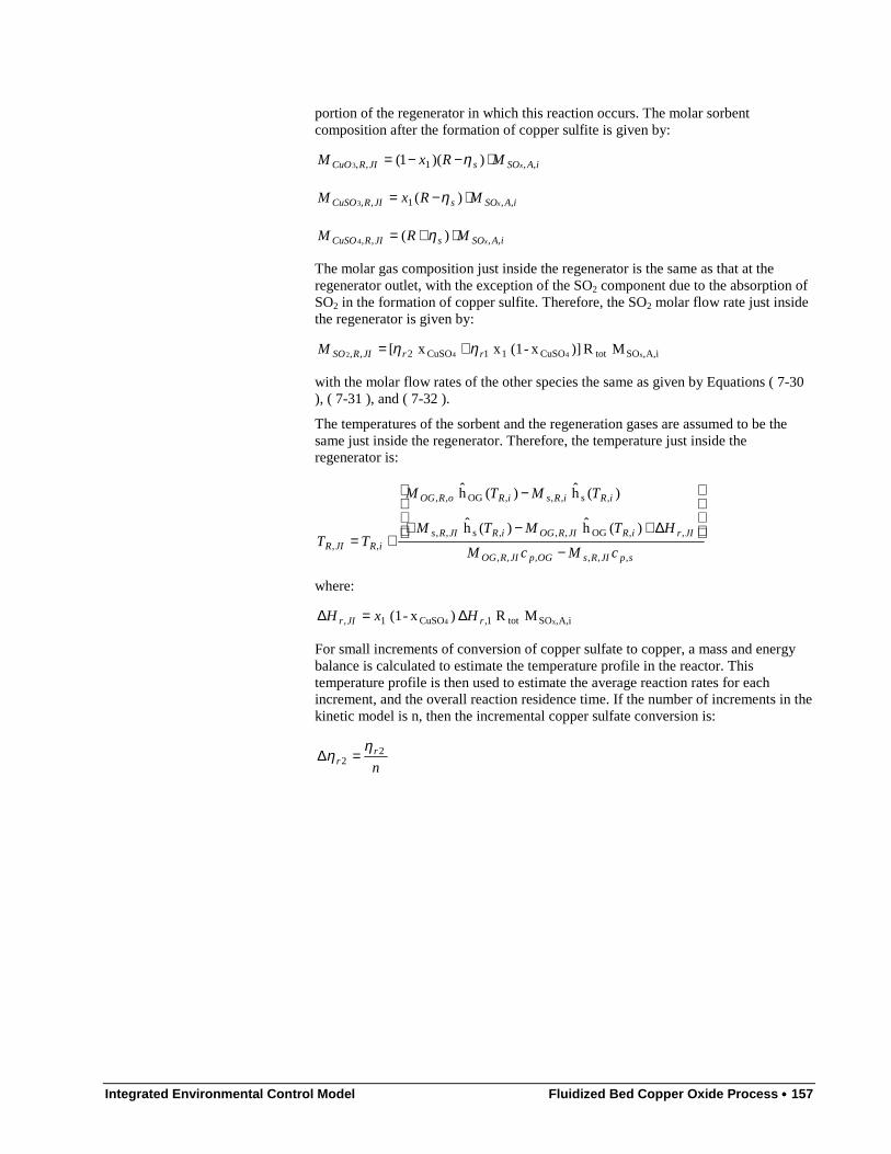
Integrated Environmental Control Model Fluidized Bed Copper Oxide Process •••• 157
portion of the regenerator in which this reaction occurs. The molar sorbentcomposition after the formation of copper sulfite is given by:
iASOsJIRCuO xMRxM ,,1,, ))(1(3 ⋅−−= η
iASOsJIRCuSO xMRxM ,,1,, )(3 ⋅−= η
iASOsJIRCuSO xMRM ,,,, )(4 ⋅+= η
The molar gas composition just inside the regenerator is the same as that at theregenerator outlet, with the exception of the SO2 component due to the absorption ofSO2 in the formation of copper sulfite. Therefore, the SO2 molar flow rate just insidethe regenerator is given by:
iA,,SOtotCuSO11CuSO2,, x442 M R )]x-(1 x x[ rrJIRSOM ηη +=
with the molar flow rates of the other species the same as given by Equations ( 7-30), ( 7-31 ), and ( 7-32 ).
The temperatures of the sorbent and the regeneration gases are assumed to be thesame just inside the regenerator. Therefore, the temperature just inside theregenerator is:
spJIRsOGpJIROG
JIriRJIROGiRJIRs
iRiRsiRoROG
iRJIR cMcM
HTMTM
TMTM
TT,,,,,,
,,OG,,,s,,
,s,,,OG,,
,,
)(h )(h
)(h )(h
−
∆+−+
−
+=
where:
iA,,SOtot1,CuSO1, x4 M R )x-(1 rJIr HxH ∆=∆
For small increments of conversion of copper sulfate to copper, a mass and energybalance is calculated to estimate the temperature profile in the reactor. Thistemperature profile is then used to estimate the average reaction rates for eachincrement, and the overall reaction residence time. If the number of increments in thekinetic model is n, then the incremental copper sulfate conversion is:
nr
r2
2η
η =∆

158 •••• Fluidized Bed Copper Oxide Process Integrated Environmental Control Model
������������������������������������������������������������������������������������������������������������������������������������������������������������������������������������������������������������������������������������������������
������������������������������������������������������������������������������������������������������������������������������������������������������������������������������������������������������������������������������������������������
SPENT SORBENT
METHANEREGENERATED SORBENT
OFF-GAS
����������������������������������������������������������������
����������������������������������������������������������������
������������������������������������������������������������������������
����������������������������������������������������������������
MCH4,R,i
TCH4,R,iMs,R,oT s,R,o
Ms,R,i
TR,i
MOG,R,i
TR,i
����������������������������������������������������������������������������������������������������������������������������������������������������������������������������������������������������������������������������������������������������������������������������������������������������������������������������������������������������������������������������������������������������������������������������������������������������������������������������������������������������������������������������������������������������������������������������������������������������������������������������������������������������������������������������������������������������������������������������������������������������������������������������������������������������������������������������������������������������������������������������������������������������������������������������������������������������������������������������������������������������������������������������������������������������������������������������������������������������������������������������������������������������������������
Just Inside
Step 1
Step 2
Step 3
Step n
• • •
TR,JI
TR,1
TR,2
TR,3
TR,n-1
M ,R,JIs
M ,R,1s
M ,R,2s
M ,R,3s
M ,R,n-1s
,R,JIMOG
,R,1MOG
,R,2MOG
,R,3MOG
,R,n-1MOG
Conversion of:
CuO to CuSO3
CuSO to Cu
4
x1
0
0
0
0
• • •
• • •
∆ηr2
∆ηr2
∆ηr2
0
2
3
ηr2
CuSO to Cu
3 CuO to Cu
0 0
∆ηr1 ∆ηr3
∆ηr1
∆ηr3
2 2
∆ηr1 ∆ηr33 3
ηr1 ηr3
• • •
• • •
Figure 7-9 Schematic of Regenerator Residence Time Model
Similarly, the conversion increments for regeneration of copper sulfite and copperoxide are assumed to be:
nr
r1
1η
η =∆
nr
r3
3η
η =∆
There are n regeneration increments. At the end of each regeneration increment, k(k=1,n), the sorbent composition is:
iASO
sCuSOr
srr
kRCu xMR
RxkM ,,
2
1113
,,)(
)]( x)1([
4
⋅
+∆+
−∆+−∆=
ηη
ηηη
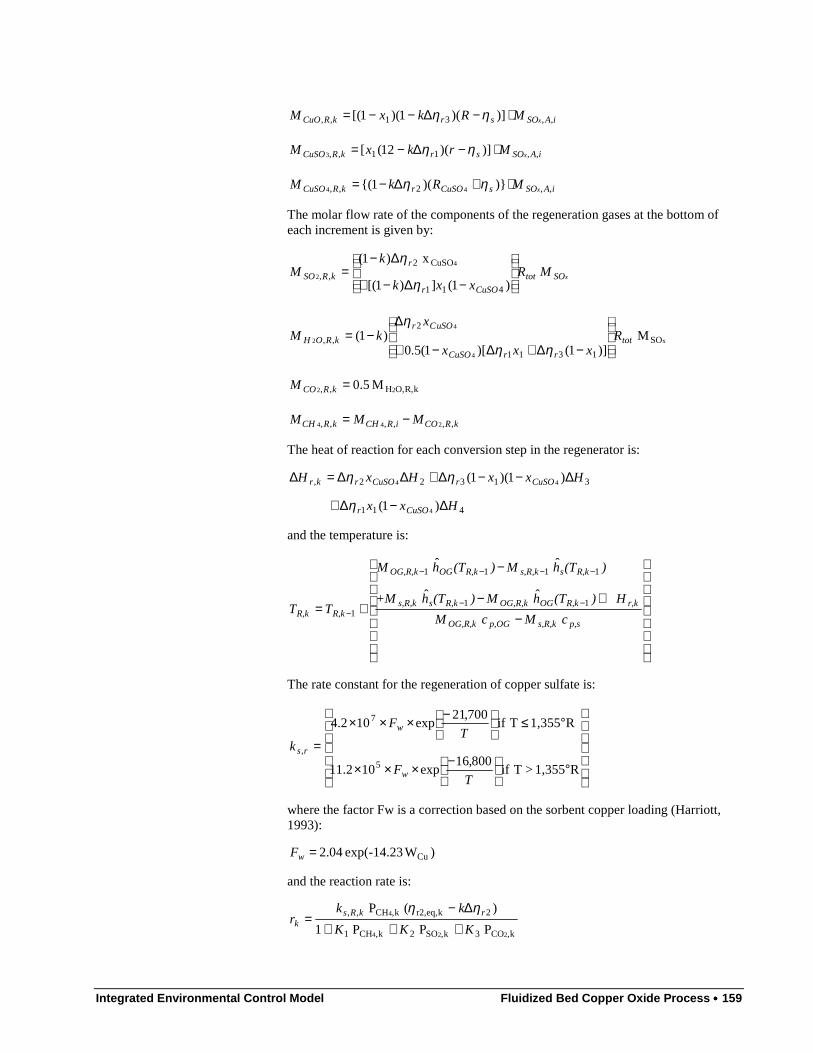
Integrated Environmental Control Model Fluidized Bed Copper Oxide Process •••• 159
iASOsrkRCuO xMRkxM ,,31,, )])(1)(1[( ⋅−∆−−= ηη
iASOsrkRCuSO xMrkxM ,,11,, )])(12([3 ⋅−∆−= ηη
iASOsCuSOrkRCuSO xMRkM ,,2,, )})(1{( 44 ⋅+∆−= ηη
The molar flow rate of the components of the regeneration gases at the bottom ofeach increment is given by:
xSOtot
CuSOr
r
kRSO MRxxk
kM
411
CuSO2
,,)1(])1[(
x)1( 4
2
−∆−+
∆−=
η
η
x
4
4
2 SO
1311
2
,, M )]1()[1(5.0
)1( tot
rrCuSO
uSOCr
kROH Rxxx
xkM
−∆+∆−+
∆−=
ηη
η
kR,O,H,, 22 M 5.0=kRCOM
kRCOiRCHkRCH MMM ,,,,,, 244 −=
The heat of reaction for each conversion step in the regenerator is:
411
31322,
)1(
)1)(1(
4
44
Hxx
HxxHxH
CuSOr
CuSOrCuSOrkr
∆−∆+
∆−−∆+∆∆=∆
η
ηη
and the temperature is:
−+−
−
+= −−
−−−−
−p,ss,R,kp,OGOG,R,k
r,kR,kOGOG,R,kR,kss,R,k
R,kss,R,kR,kOGOG,R,k
R,kR,k cM cM
H)(Th M)(Th +M
)(Th M)(Th M
TT 11
1111
1
ˆˆ
ˆˆ
The rate constant for the regeneration of copper sulfate is:
°
−×××
°≤
−×××
=
R1,355>T if 800,16
exp1011.2
R1,355T if 700,21
exp102.4
5
7
,
TF
TF
k
w
w
rs
where the factor Fw is a correction based on the sorbent copper loading (Harriott,1993):
) Wexp(-14.23 04.2 Cu=wF
and the reaction rate is:
k,CO3k,SO2k,CH1
2keq,r2,k,CH,,
224
4
P P P 1
)( P
KKK
kkr
rkRsk +++
∆−=
ηη
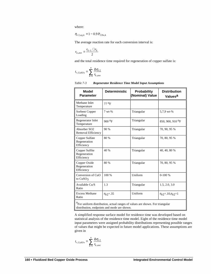
160 •••• Fluidized Bed Copper Oxide Process Integrated Environmental Control Model
where:
k,CH,,2 4P 9.01−=keqrη
The average reaction rate for each conversion interval is:
21
,kk
avekrr
r+
= −
and the total residence time required for regeneration of copper sulfate is:
∑=
∆=n
k avek
rCuSOr r
t1 ,
2, 4
η
Table 7-3 Regenerator Residence Time Model Input Assumptions
ModelParameter
Deterministic Probability(Nominal) Value
DistributionValues a
Methane InletTemperature
77 oF
Sorbent CopperLoading
7 wt-% Triangular 5,7,9 wt-%
Regenerator InletTemperature
900 oF Triangular 850, 900, 910 oF
Absorber SO2Removal Efficiency
90 % Triangular 70, 90, 95 %
Copper SulfateRegenerationEfficiency
80 % Triangular 70, 80, 95 %
Copper SulfiteRegenerationEfficiency
40 % Triangular 40, 40, 80 %
Copper OxideRegenerationEfficiency
80 % Triangular 70, 80, 95 %
Conversion of CuOto CuSO3
100 % Uniform 0-100 %
Available Cu/SRatio
1.3 Triangular 1.5, 2.0, 3.0
Excess MethaneRatio
ηr2+.35 Uniform ηr2+.10,ηr2+1
aFor uniform distribution, actual ranges of values are shown. For triangular
distribution, endpoints and mode are shown.
A simplified response surface model for residence time was developed based onstatistical analysis of the residence time model. Eight of the residence time modelinput parameters were assigned probability distributions representing possible rangesof values that might be expected in future model applications. These assumptions aregiven in
∑=
∆=n
k avek
rCuSOr r
t1 ,
2, 4
η

Integrated Environmental Control Model Fluidized Bed Copper Oxide Process •••• 161
Table 7-3. These distributions were sampled using Latin Hypercube sampling, avariant of Monte Carlo simulation, and the paired sets of sample values were used tocalculate the corresponding residence times. A total of 100 sets of calculations weremade. Linear regression analysis was used to correlated the resulting distribution ofresidence time values to each of the input distributions. The simplified model forregenerator residence time is:
}03.139.044.076.3
90.0009.010.031.8exp{01.1
412
,,4,
CHr
siRsCuCuSOr
RRx
tWt
−−−+
+−+⋅=
η
η( 7-33 )
This regression model has a coefficient of determination (R2) of 0.95. The standarderror of the estimate of residence time is 1 minute. This model should not beextrapolated.
7.3.4. ByProduct RecoveryThe regenerator off-gas is sent to a byproduct recovery plant for processing. Aspreviously noted, elemental sulfur recovery using a Claus plant is the design basisfor this study. A two-stage Allied Chemical design is assumed, based on previousstudies (Ratafia-Brown, 1983; Rubin et al., 1991). The sulfur recovery efficiency forthis design is estimated to be 95 percent, with the unconverted sulfur emitted as SO2
in the Claus plant tailgas. Thus, the overall sulfur removal efficiency if the copperoxide process removes 90 percent of sulfur oxides from the flue gas would be only85.5 percent. Such a design is likely to be unacceptable compared to conventionalflue gas desulfurization systems, which are capable of 90 percent or greater sulfurcapture.
Three approaches are possible to improve the overall system SOx removal efficiency.These are: (1) increase the copper oxide removal efficiency to compensate for theClaus plant tailgas emissions; (2) recycle the tailgas emissions to the flue gasupstream of the fluidized bed absorber, and adjust the copper oxide removalefficiency; or (3) increase the sulfur capture efficiency of the Claus plant. The thirdoption is not considered here, due to the need to obtain detailed design informationthat is not readily available. However, the first two options are considered in thecopper oxide process performance model.
The first approach is easily modeled by adjusting the copper oxide sulfur oxidescapture efficiency based on the sulfur recovery plant efficiency:
Claus
overallss η
ηη ,=
For example, if an overall removal efficiency of 90 percent is required, and if theClaus plant recovers only 95 percent of the sulfur in the regenerator offgas, then thecopper oxide process sulfur removal efficiency must be 94.7 percent. Such anincrease in removal efficiency will substantially increase the sorbent requirement.Depending on the design assumptions, an increase sorbent circulation rate of over 40percent may be required. Therefore, it is unlikely that this is the lowest costapproach.
The second approach is modeled by injecting into the flue gas just upstream of thefluidized bed absorber an amount of SO2 equivalent to the sulfur molar flow in theClaus plant tailgas:
FGSOsClaus
sClausrecycleSO MM ,, 22 )1(1
)1(
−−−
=ηη
ηη
162 •••• Fluidized Bed Copper Oxide Process Integrated Environmental Control Model
The required absorber sulfur removal efficiency is given by:
overallsClausClaus
overallss
,
,
)1( ηηηη
η−+
=
In contrast to the example given above, the sulfur removal efficiency in the absorberis only 90.45 percent. Combined with the increased sulfur loading to the absorber,the tailgas recycle approach results in a modest increase in the sorbent circulationrate of typically less than 10 percent.
As part of process integration, the regeneration offgas must be dried and cooled priorto entering the sulfur recovery plant (Ratafia-Brown, 1983). A typical regeneratoroffgas is at a temperature of 875 to 910°F, with a moisture content of 40 to 45percent. The design basis for gas inlet to the Claus plant calls for a temperature of500°F with a moisture content of only 6 percent. The net effect of the gas treatmentand cooling is to generate superheated steam, which may be used elsewhere in thepower plant.
7.3.5. Energy Penalties and CreditsThe copper oxide process consumes electrical energy to operate blowers andcompressors associated with the pneumatic solids transport system and thecombustor for the sorbent heater. Due to the flue gas pressure drop across thefluidized bed absorber, additional electrical energy is required to operate the powerplant induced draft fan. The sulfur recovery system consumes a relatively smallamount of power.
The electrical requirements of the various fans are estimated using the "fan equation"(McQuiston and Parker, 1982):
fanfan
PQEC
η512,8
∆=
The fan efficiencies are assumed to be 85 percent. For the induced draft fan, theincremental pressure drop is estimated based on the fluidized bed height. For a 48inch bed height, the pressure drop is approximately 28 inches of water (Frey, 1987).For the dense phase solids transport system between the regenerator and theabsorber, the pressure drop is 22 psi (Roberts and Schaeffer, 1992). The pressuredrop across the sorbent transport system between the absorber and the solids heater isestimated at 4.3 psi (Ratafia-Brown, 1983). The pressure drop across the solidsheater combustor is estimated at 90 inches of water (Ratafia-Brown, 1983).
The copper oxide process and the sulfur recovery plant utilize methane for solidsheating, sorbent regeneration, and regenerator offgas reduction. The methanerepresents an energy input into the power plant system.
Due to the exothermic reactions occurring in the fluidized bed absorber, as well as tothe thermal energy added to the sorbent during solids heating, the temperature of theflue gas exiting the absorber is substantially higher than the inlet temperature. Thetemperature increase is typically on the order of 100°F. This additional energy maybe recovered by the power plant air preheater, and used to increase the temperatureof the combustion air entering the boiler. The calculation of this energy credit isdescribed by Rubin et al. (1991, pp. 27, 44-46).
The copper oxide process uses steam for ammonia vaporization and injection.However, the offgas pretreatment section of the sulfur recovery plant producessteam, as previously described. Typically, the net effect is an energy credit. Thethermal value of the steam is converted to an electricity equivalent basis using the

Integrated Environmental Control Model Fluidized Bed Copper Oxide Process •••• 163
power plant gross steam cycle heat rate (excluding the boiler, see Rubin et al., 1991,p. 45 for details).
7.4. Cost ModelThis section presents the economic model developed for the fluidized bed copperoxide process. The source of economic data for this model includes previous workby Frey (1987; 1991) as well as new data developed by A.E. Roberts and Associates(1994). The cost model is comprised of a capital cost model and an annual costmodel.
7.4.1. Capital Cost ModelsThe capital cost of a complete fluidized bed copper oxide system includes thefollowing major equipment items:
• Fluidized bed absorbers
• Ammonia Injection System
• Regenerator
• Solids Heater
• Sorbent Transport System
• Byproduct Recovery System
For each of these major systems, a direct capital cost model is developed.
7.4.1.1. Fluidized Bed AbsorbersThe direct capital cost of the fluidized bed absorbers includes the absorber vessel,structural supports, dampers and isolation valves, refractory lining for the inside ofthe absorber, ductwork, instrumentation and control, and installation costs.
The absorber vessels are refractory-lined carbon steel of minimum one-half inchthickness. Each absorber vessel may be approximated as a cylinder. The internaldiameter of the absorber vessel is determined based on the superficial gas velocityrequirement. The materials cost of the absorber are proportional to the surface areaof the absorber vessel.
The absorber vessel internal radius is given by:
Oas
FGa NV
Gr
, 60π=
The diameter of the absorber vessel must be larger than this internal radius toaccommodate the thickness of refractory lining. The design basis developed by A. E.Roberts and Associates (AERA) for the absorber includes a two-inch thick base orinner refractory covering the internal surface of the absorber vessel. A second "hotbase" refractory layer approximately six inches thick is placed over the first layer.Thus, the vessel internal diameter is:
hriraav ttrr ++=,
The surface area of the absorber vessel is approximated by the following equation forthe surface area of a cylinder:

164 •••• Fluidized Bed Copper Oxide Process Integrated Environmental Control Model
aavava hrrSA ,2
, 2)(2 ππ +=
The design height of the absorber vessel is approximately 70 feet, based on theAERA design basis. The total height of the absorber assembly is larger when flue gasoutlet ductwork is taken into consideration. The straight wall portion of the absorbervessel that is covered with refractory lining is approximately 35 feet.
The direct cost for the steel absorber vessel is estimated based on the ratio of surfaceareas referenced to a base case design. The AERA design is predicated on a flue gasvolumetric flow rate of 500,000 scfm at 705°F and a superficial gas velocity of 4.5ft/sec. Therefore, the required internal radius is 36.4 feet. Accounting for the 8 inchtotal thickness of the refractory, the steel vessel's internal diameter must be 37 feet.Therefore, the approximate surface area of the absorber vessel is 24,875 ft2. The basecost estimate is $1,434,000 (in 1993 dollars) for a single absorber vessel of this size.Therefore, the direct cost model for the cost of the steel absorber vessel is given by:
PCI 1993
PCI
ft 875,24N 434,1
2Ta,,
= SA
DC va
Typically, there will be two 50% capacity absorber vessels with no spares. The costof refractory is given by the refractory surface area, required to cover the sides of theabsorber vessel, and a unit cost for refractory per square foot:
rTaswaara UCNhrDC ,,, 2π=
In 1993, the unit cost of the total of 8 inches of refractory required for the absorberwas approximately $55/ft2.
Each absorber requires structural supports. In the base case design, these areestimated at $100,000 per vessel. The structural support is assumed here to havesome economy of scale with respect to size. As a default assumption, a six-tenthsscaling rule is assumed:
PCI 1993
PCI
ft 875,24N 100
0.6
2Ta,,
= a
saSA
DC
The surface area of the absorber vessel is used as a surrogate variable for the size ofthe absorber system and, hence, the proportional size of the structural supports.
The costs for flue gas ductwork, flue gas isolation valves, and dampers are assumedto be proportional to the flue gas volumetric flow rate. Moreover, economies of scaleare assumed. In the absence of more detailed information, the following direct costmodel was developed:
×=
Oa,36Ta,,
N min/101.1N 300
ft
GDC FG
da
In this model, the cost of ductwork, isolation valves, and dampers is estimated for asingle absorber vessel, and is multiplied by the total number of absorber vessels.
The total direct cost for the absorber process area is given by:
))(1( ,,,,, dasaravaaica DCDCDCDCfDC ++++=
where fic,a is an installation cost factor for the absorber process area. A default valueof 0.45 is suggested.
Integrated Environmental Control Model Fluidized Bed Copper Oxide Process •••• 165
In addition to these direct costs, there is an incremental cost associated withincreasing the pressure drop of the flue gas. The differential cost required to"modify" a new induced draft fan has been modeled by Frey (1994). The energyrequirement required to overcome the absorber flue gas pressure drop is:
Oa,, N 512,8 fan
CuOFGdifID
PGEC
η∆
=
The fan efficiency is typically 85 percent. The cost of the ID fan differential is:
=
3.357600,4 N 180
6.0,
Ta,,PCIEC
DCdifID
difID
7.4.1.2. Ammonia Injection SystemAmmonia is injected into the flue gas upstream of the absorber vessel. The ammoniainjection system is comprised of the following equipment, based on the AERAdesign basis:
• One ammonia storage tank per absorber vessel, plus one common sparetank
• One air compressor per storage tank
• One vaporizer per absorber vessel
• Injection probes and nozzles for each absorber inlet
• Control panels
The cost of the ammonia injection system is most sensitive to the ammonia flow raterequirement for each absorber vessel. The ammonia flow rate requirement dependson the NOx loading into the absorbers and the ammonia-to-NOx molar ratio requiredto achieve a given level of NOx control. The total ammonia mass flow rate is givenby:
xNONHNHNH MRMWm 333 =
Storage to provide 30 days supply of ammonia is required under the design basis.The total ammonia storage requirement is distributed among several tanks,depending on how many absorber vessels are used. Therefore, the storage capacity ofeach tank is given by:
)1(N lb/gallon) (8.34
D 24
Oa,
NH333 +
= NHNH
mC
Based on Perry's Chemical Engineer's Handbook (6th Ed., p. 25-69), the exponentialfactor appropriate for horizontal tanks is 0.57. Based on a previous cost estimatedeveloped by AERA, the cost of an 80,000 gallon ammonia storage tank isapproximately $235,000. Therefore, the storage tank cost is given by:
PCI 1993
PCI
80,000
C )1(N 235 )1(
57.0NH
,,,3
++= OaaiicSai fDC
The detailed costs for other components of the ammonia injection system are notdisaggregated in the AERA cost estimate. However, based on a previous AERAestimate, the total cost of the ammonia injection system was estimated as $2.3million. This estimate was for an ammonia flow rate of 1,751 lb/hr, but involved
166 •••• Fluidized Bed Copper Oxide Process Integrated Environmental Control Model
three 80,000 gallon storage tanks. Assuming an installation cost factor of 45 percentfor the storage tanks, the net installed cost of the ammonia vaporization and injectionsystem is $1.28 million. This cost should scale with the ammonia flow rate. Frey(1994) developed a direct cost model of an ammonia injection system for selectivecatalytic reduction (SCR) in which the scaling exponent was found to be 0.482.Therefore, the direct cost for the ammonia vaporization and injection components isestimated as:
PCI 1993
PCI ))((5.17 482.0
,, 3NHTavai mNDC −
The direct cost of the ammonia injection system is therefore:
vaiSaiai DCDCDC ,, +=
7.4.1.3. RegeneratorThe regenerator is a carbon steel cylindrical vessel. The regenerator is sized toaccommodate sorbent storage for a specified sorbent residence time. In the base case,AERA has designed a regenerator with a sorbent hold-up volume of 8,800 ft3. Theregenerator design features a 28 foot straight wall height. Here, it is assumed that thestraight wall height is held fixed, and the radius is adjusted to accommodate variousresidence times.
The required regenerator radius is therefore given by:
swR
RiRsR h
tmr
,OR,s
,,
N 60 πρ=
The total height of the regenerator is the straight wall height plus inlet and outletclearances for gas flows. These clearances add approximately 17 feet to the straightwall height. The inside of the regenerator vessel walls are covered with two layers ofrefractory totaling 8 inches in thickness. Therefore, the steel vessel diameter is
hrirRRv ttrr ++=,
The surface area of the regenerator vessel is approximated by the surface area of acylinder:
RRvRvR hrrSA ,2
, 2)(2 ππ +=
In the base case, the regenerator has an equivalent overall height of 78 feet and aradius of 10 feet. The direct cost of the regenerator vessel is:
PCI 1993
PCI
ft 530,5N 475
2Ra,,
= R
vRSA
DC
The direct cost of refractory is given by:
rTRRRrR UCNhrDC ,, 2π=
Each regenerator requires structural supports. In the base case design, these areestimated at $42,500 per vessel. The structural support is assumed here to have someeconomy of scale with respect to size. As a default assumption, a six-tenths scalingrule is assumed:
Integrated Environmental Control Model Fluidized Bed Copper Oxide Process •••• 167
PCI 1993ft 530,5N 5.42
0.6
2Ta,,PCISA
DC asR
=
The surface area of the absorber vessel is used as a surrogate variable for the size ofthe regenerator system and, hence, the proportional size of the structural supports.
The costs for ductwork, isolation valves, and dampers are assumed to be proportionalto the regenerator offgas volume flow rate. Moreover, economies of scale areassumed. In the base case analysis, approximately 1,300 lbmole/hour of offgas is
evolved from the regenerator. At 900 oF, the volumetric flow rate is 21,900 ft3/min.Thus, in the absence of more detailed information, the following direct cost modelwas developed:
PCI 1993
PCI
Nlbmole/hr 626N 350
6.0
OR,TR,,
= OG
dRG
DC
In this model, the cost of ductwork, isolation valves, and dampers is estimated for asingle absorber vessel, multiplied by the total number of absorber vessels.
A methane feed system and a booster compressor and motor is required for the inletmethane to overcome the pressure drop through the regenerator. The boostercompressor cost is assumed to be proportional to the methane flow rate. The costequation is thus:
PCI 1993Nlbmole/hr 187N 350
6.0
OR,
,,TR,,
4 PCIMDC
iRCHbfR
=
The total direct cost for the absorber process area is given by:
))(1( ,,,,,, bfRdRsRrRvRRicR DCDCDCDCDCfDC +++++=
where fic,R is an installation cost factor for the absorber process area. A defaultvalue of 0.45 is suggested.
7.4.1.4. Solids HeaterThe solids heater is a carbon steel cylindrical vessel. In the base case, AERA hasdesigned a solids heater with an internal radius of 10 feet and a height of 50 feet. Theside walls of the heater are lined with refractory material. The internal diameter ofthe solids heater is proportional to the mass flow of sorbent entering the vessel. Thevessel contains two sorbent beds in which hot combustion gases from a methanecombustor contact the sorbent in counter-current flow. Thus, for fixed bed heights ineach stage, the solids heater internal radius varies with the sorbent mass flow rate asfollows:
OSH,
,,
N 000,40010 iSHs
SH
mr =
The inside of the solids heater vessel walls are covered with two layers of refractorytotaling 8 inches in thickness. Therefore, the steel vessel diameter is
hrirSHSHv ttrr ++=,
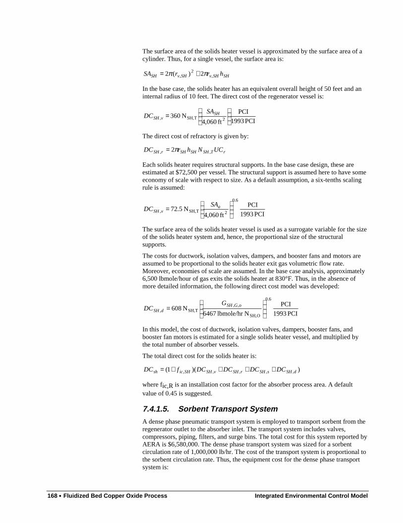
168 •••• Fluidized Bed Copper Oxide Process Integrated Environmental Control Model
The surface area of the solids heater vessel is approximated by the surface area of acylinder. Thus, for a single vessel, the surface area is:
SHSHvSHvSH hrrSA ,2
, 2)(2 ππ +=
In the base case, the solids heater has an equivalent overall height of 50 feet and aninternal radius of 10 feet. The direct cost of the regenerator vessel is:
PCI 1993
PCI
ft 060,4N 360
2TSH,,
= SH
vSHSA
DC
The direct cost of refractory is given by:
rTSHSHSHrSH UCNhrDC ,, 2π=
Each solids heater requires structural supports. In the base case design, these areestimated at $72,500 per vessel. The structural support is assumed here to have someeconomy of scale with respect to size. As a default assumption, a six-tenths scalingrule is assumed:
PCI 1993
PCI
ft 060,4N 5.72
0.6
2TSH,,
= a
vSHSA
DC
The surface area of the solids heater vessel is used as a surrogate variable for the sizeof the solids heater system and, hence, the proportional size of the structuralsupports.
The costs for ductwork, isolation valves, dampers, and booster fans and motors areassumed to be proportional to the solids heater exit gas volumetric flow rate.Moreover, economies of scale are assumed. In the base case analysis, approximately6,500 lbmole/hour of gas exits the solids heater at 830°F. Thus, in the absence ofmore detailed information, the following direct cost model was developed:
PCI 1993
PCI
Nlbmole/hr 6467N 608
0.6
OSH,
,,TSH,,
= oGSH
dSH
GDC
In this model, the cost of ductwork, isolation valves, dampers, booster fans, andbooster fan motors is estimated for a single solids heater vessel, and multiplied bythe total number of absorber vessels.
The total direct cost for the solids heater is:
))(1( ,,,,, dSHsSHrSHvSHSHicsh DCDCDCDCfDC ++++=
where fic,R is an installation cost factor for the absorber process area. A defaultvalue of 0.45 is suggested.
7.4.1.5. Sorbent Transport SystemA dense phase pneumatic transport system is employed to transport sorbent from theregenerator outlet to the absorber inlet. The transport system includes valves,compressors, piping, filters, and surge bins. The total cost for this system reported byAERA is $6,580,000. The dense phase transport system was sized for a sorbentcirculation rate of 1,000,000 lb/hr. The cost of the transport system is proportional tothe sorbent circulation rate. Thus, the equipment cost for the dense phase transportsystem is:
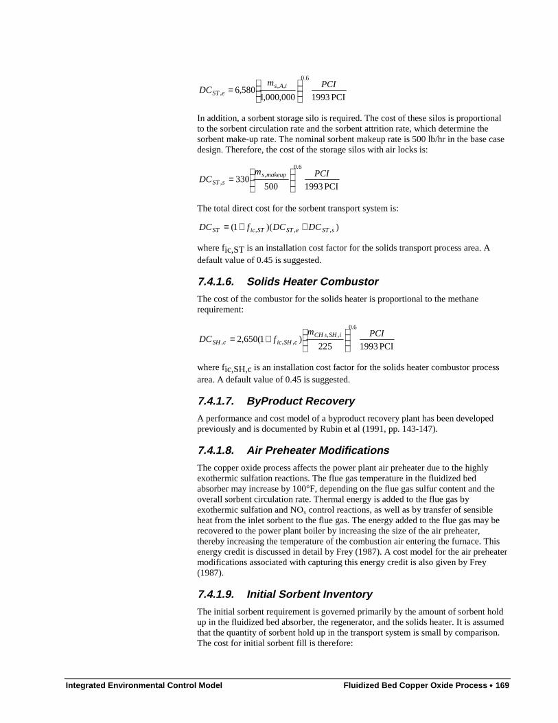
Integrated Environmental Control Model Fluidized Bed Copper Oxide Process •••• 169
PCI 1993000,000,1580,6
6.0,,
,PCIm
DC iAseST
=
In addition, a sorbent storage silo is required. The cost of these silos is proportionalto the sorbent circulation rate and the sorbent attrition rate, which determine thesorbent make-up rate. The nominal sorbent makeup rate is 500 lb/hr in the base casedesign. Therefore, the cost of the storage silos with air locks is:
PCI 1993500330
6.0,
,PCIm
DCmakeups
sST
=
The total direct cost for the sorbent transport system is:
))(1( ,,, sSTeSTSTicST DCDCfDC ++=
where fic,ST is an installation cost factor for the solids transport process area. Adefault value of 0.45 is suggested.
7.4.1.6. Solids Heater CombustorThe cost of the combustor for the solids heater is proportional to the methanerequirement:
PCI 1993225)1(650,2
6.0,,
,,,4 PCIm
fDCiSHCH
cSHiccSH
+=
where fic,SH,c is an installation cost factor for the solids heater combustor processarea. A default value of 0.45 is suggested.
7.4.1.7. ByProduct RecoveryA performance and cost model of a byproduct recovery plant has been developedpreviously and is documented by Rubin et al (1991, pp. 143-147).
7.4.1.8. Air Preheater ModificationsThe copper oxide process affects the power plant air preheater due to the highlyexothermic sulfation reactions. The flue gas temperature in the fluidized bedabsorber may increase by 100°F, depending on the flue gas sulfur content and theoverall sorbent circulation rate. Thermal energy is added to the flue gas byexothermic sulfation and NOx control reactions, as well as by transfer of sensibleheat from the inlet sorbent to the flue gas. The energy added to the flue gas may berecovered to the power plant boiler by increasing the size of the air preheater,thereby increasing the temperature of the combustion air entering the furnace. Thisenergy credit is discussed in detail by Frey (1987). A cost model for the air preheatermodifications associated with capturing this energy credit is also given by Frey(1987).
7.4.1.9. Initial Sorbent InventoryThe initial sorbent requirement is governed primarily by the amount of sorbent holdup in the fluidized bed absorber, the regenerator, and the solids heater. It is assumedthat the quantity of sorbent hold up in the transport system is small by comparison.The cost for initial sorbent fill is therefore:
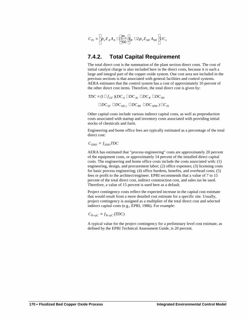
170 •••• Fluidized Bed Copper Oxide Process Integrated Environmental Control Model
sSHSHsRs
AAsIS UCAZtm
AZC
+
+= ρρ 260
7.4.2. Total Capital RequirementThe total direct cost is the summation of the plant section direct costs. The cost ofinitial catalyst charge is also included here in the direct costs, because it is such alarge and integral part of the copper oxide system. One cost area not included in theprevious sections is that associated with general facilities and control systems.AERA estimates that the control system has a cost of approximately 10 percent ofthe other direct cost items. Therefore, the total direct cost is given by:
ISAPHBYcSHST
SHRAIAGF
CDCDCDCDC
DCDCDCDCfTDC
+++++
++++=
)
)(1(
,
Other capital costs include various indirect capital costs, as well as preproductioncosts associated with startup and inventory costs associated with providing initialstocks of chemicals and fuels.
Engineering and home office fees are typically estimated as a percentage of the totaldirect cost:
TDCfC EHOEHO =
AERA has estimated that "process engineering" costs are approximately 20 percentof the equipment costs, or approximately 14 percent of the installed direct capitalcosts. The engineering and home office costs include the costs associated with: (1)engineering, design, and procurement labor; (2) office expenses; (3) licensing costsfor basic process engineering; (4) office burdens, benefits, and overhead costs; (5)fees or profit to the architect/engineer. EPRI recommends that a value of 7 to 15percent of the total direct cost, indirect construction cost, and sales tax be used.Therefore, a value of 15 percent is used here as a default.
Project contingency costs reflect the expected increase in the capital cost estimatethat would result from a more detailed cost estimate for a specific site. Usually,project contingency is assigned as a multiplier of the total direct cost and selectedindirect capital costs (e.g., EPRI, 1986). For example:
)(PrPr TDCfC ojCojC =
A typical value for the project contingency for a preliminary level cost estimate, asdefined by the EPRI Technical Assessment Guide, is 20 percent.
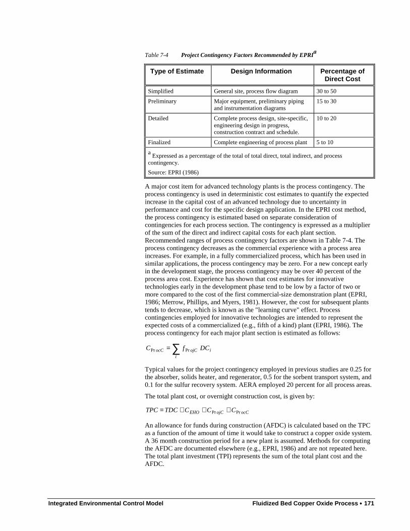
Integrated Environmental Control Model Fluidized Bed Copper Oxide Process •••• 171
Table 7-4 Project Contingency Factors Recommended by EPRIa
Type of Estimate Design Information Percentage ofDirect Cost
Simplified General site, process flow diagram 30 to 50
Preliminary Major equipment, preliminary pipingand instrumentation diagrams
15 to 30
Detailed Complete process design, site-specific,engineering design in progress,construction contract and schedule.
10 to 20
Finalized Complete engineering of process plant 5 to 10
a Expressed as a percentage of the total of total direct, total indirect, and process
contingency.
Source: EPRI (1986)
A major cost item for advanced technology plants is the process contingency. Theprocess contingency is used in deterministic cost estimates to quantify the expectedincrease in the capital cost of an advanced technology due to uncertainty inperformance and cost for the specific design application. In the EPRI cost method,the process contingency is estimated based on separate consideration ofcontingencies for each process section. The contingency is expressed as a multiplierof the sum of the direct and indirect capital costs for each plant section.Recommended ranges of process contingency factors are shown in Table 7-4. Theprocess contingency decreases as the commercial experience with a process areaincreases. For example, in a fully commercialized process, which has been used insimilar applications, the process contingency may be zero. For a new concept earlyin the development stage, the process contingency may be over 40 percent of theprocess area cost. Experience has shown that cost estimates for innovativetechnologies early in the development phase tend to be low by a factor of two ormore compared to the cost of the first commercial-size demonstration plant (EPRI,1986; Merrow, Phillips, and Myers, 1981). However, the cost for subsequent plantstends to decrease, which is known as the "learning curve" effect. Processcontingencies employed for innovative technologies are intended to represent theexpected costs of a commercialized (e.g., fifth of a kind) plant (EPRI, 1986). Theprocess contingency for each major plant section is estimated as follows:
∑=i
iojCocC DCfC PrPr
Typical values for the project contingency employed in previous studies are 0.25 forthe absorber, solids heater, and regenerator, 0.5 for the sorbent transport system, and0.1 for the sulfur recovery system. AERA employed 20 percent for all process areas.
The total plant cost, or overnight construction cost, is given by:
ocCojCEHO CCCTDCTPC PrPr +++=
An allowance for funds during construction (AFDC) is calculated based on the TPCas a function of the amount of time it would take to construct a copper oxide system.A 36 month construction period for a new plant is assumed. Methods for computingthe AFDC are documented elsewhere (e.g., EPRI, 1986) and are not repeated here.The total plant investment (TPI) represents the sum of the total plant cost and theAFDC.
172 •••• Fluidized Bed Copper Oxide Process Integrated Environmental Control Model
The final measure of capital cost is the total capital requirement (TCR). The TCRincludes the total plant investment plus costs for royalties, startup costs, and initialinventories of feed stocks. In this case, no costs are assumed for royalties.Preproduction costs typically include one month of both fixed and variable operatingcosts and two percent of total plant investment. Inventory capital is estimated as 0.5percent of total process capital excluding catalyst. The costs for initial catalysts andchemicals is zero. The copper oxide initial sorbent requirement is included in theprocess capital costs. Thus, for a copper oxide system, the total capital requirementis:
∑++++=i
iICPP DCfTPIfFOCVOC
TCR )1(12
7.4.3. Annual CostsThe annual costs for copper oxide systems include fixed and variable operating costs.Fixed operating costs include operating labor, maintenance labor and materials, andoverhead costs associated with administrative and support labor. Variable operatingcosts include consumables, such as ammonia and sorbent replacement. Costs forsteam and electricity consumed from within the plant may also be estimated.
7.4.3.1. Fixed Operating CostsFixed operating costs include operating labor, maintenance labor and materials, andoverhead costs associated with administrative and support labor. The operating laborcost is based on an estimate of the number of personnel hours required to operate theplant multiplied by an average labor rate. It is common to assume that four shifts perday are required for plant operation, allowing two hours overlap for transitionbetween shifts. Furthermore, an allowance for personnel on sick leave or vacationcan be incorporated into the "shift factor." A shift factor of 4.75 is assumed as adefault in this study, based on Bechtel (1988).
The number of operators required per shift for the copper oxide process is estimatedby AERA to be five. The total operating labor cost is estimated by summing thenumber of plant operators per shift for all process areas, applying the shift factor, andapplying the average labor rate as follows:
)N 21(yr
080,2OA,+= SF
hrsALROCL
The cost for maintenance material and labor for new technologies is typicallyestimated as a percentage of the installed capital cost for each process section. Thetotal maintenance cost for the plant is given by:
TPCfOC MM =
where a typical value of the maintenance cost multiplier, fM, is 0.045 for a solidshandling system. The total maintenance operating cost may be disaggregated intomaterial and labor components using the following approach:
MOC 60.0=MMOC
MOC 40.0=MLOC
The administrative and support labor cost is assumed to be 30 percent of theoperating and maintenance labor cost:

Integrated Environmental Control Model Fluidized Bed Copper Oxide Process •••• 173
)( 30.0 MLLAS OCOCOC +=
7.4.3.2. Variable Operating CostsThe variable operating costs include all consumable materials required for operationof the plant. These include the costs of sorbent for makeup of attrition losses, the costof ammonia for injection into the fluidized bed absorber, and the cost of methanerequired for regeneration and solids heating. In addition, the electricity and steamconsumption of the copper oxide process results in an energy penalty. However, theincreased flue gas temperature in the fluidized bed absorber results in an energycredit.
The annual costs for sorbent makeup, ammonia, and methane consumption are givenby:
smakeupss UCmVOC ,fc 760,8=
333 ,,fc 760,8 NHiANHNH UCmVOC =
44444 )(c 760,8 ,,,f CHBYCHRCHSHCHCH UCmmmVOC ++=
Note that methane is required for solids heating, as a reducing gas for theregeneration reactions, and also as a reducing gas for off-gas pretreatment in theClaus plant.
The variable operating costs also include a byproduct credit for the sale of elementalsulfur produced by the Claus plant. The amount of this credit is given by:
SBYBY UCVOC
=
000,2
M 32c 760,8 oR,,SO
f2η
A variable operating cost credit is also taken for a reduction in coal consumptionassociated with the increased combustion air inlet temperature, which in turn resultsfrom the higher flue gas temperature entering the air preheater. This credit isdiscussed by Frey (1987).
7.5. Sensitivity Analyses of the Fluidized Bed CopperOxide Process
The copper oxide process performance and economic models are applied to severalcase studies to identify key process sensitivities and to identify potentially robustdesign configurations. These analysis are predicated on "deterministic" analyses, inwhich point-estimates are used for all model input parameters. In the followingchapter, uncertainties in the copper oxide process will be quantified and evaluated.
7.5.1. Integration of copper oxide process andbyproduct recovery system
The copper oxide process performance model is applied here to three case studies tocompare alternative approaches for dealing with the Claus plant tailgas. The designbasis is a 500 MW power plant. The coal composition and the calculated flow rateare given in Table 7-5, the calculated flue gas composition and flow upstream of thecopper oxide process are given in Table 7-6, and the key design assumptions and
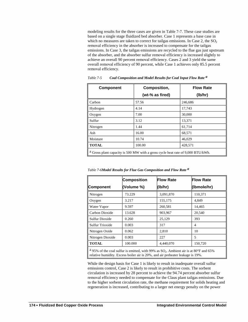
174 •••• Fluidized Bed Copper Oxide Process Integrated Environmental Control Model
modeling results for the three cases are given in Table 7-7. These case studies arebased on a single stage fluidized bed absorber. Case 1 represents a base case inwhich no measures are taken to correct for tailgas emissions. In Case 2, the SO2
removal efficiency in the absorber is increased to compensate for the tailgasemissions. In Case 3, the tailgas emissions are recycled to the flue gas just upstreamof the absorber, and the absorber sulfur removal efficiency is increased slightly toachieve an overall 90 percent removal efficiency. Cases 2 and 3 yield the sameoverall removal efficiency of 90 percent, while Case 1 achieves only 85.5 percentremoval efficiency.
Table 7-5 Coal Composition and Model Results for Coal Input Flow Rate a
Component Composition,
(wt-% as fired)
Flow Rate
(lb/hr)
Carbon 57.56 246,686
Hydrogen 4.14 17,743
Oxygen 7.00 30,000
Sulfur 3.12 13,371
Nitrogen 1.44 61,714
Ash 16.00 68,571
Moisture 10.74 46,029
TOTAL 100.00 428,571
a Gross plant capacity is 500 MW with a gross cycle heat rate of 9,000 BTU/kWh.
Table 7-6Model Results for Flue Gas Composition and Flow Rate a
Component
Composition
(Volume %)
Flow Rate
(lb/hr)
Flow Rate
(lbmole/hr)
Nitrogen 73.229 3,091,870 110,371
Oxygen 3.217 155,175 4,849
Water Vapor 9.597 260,581 14,465
Carbon Dioxide 13.628 903,967 20,540
Sulfur Dioxide 0.260 25,129 393
Sulfur Trioxide 0.003 317 4
Nitrogen Oxide 0.062 2,810 10
Nitrogen Dioxide 0.003 227 5
TOTAL 100.000 4,440,070 150,720
a 95% of the coal sulfur is emitted, with 99% as SO2. Ambient air is at 80°F and 65%relative humidity. Excess boiler air is 20%, and air preheater leakage is 19%.
While the design basis for Case 1 is likely to result in inadequate overall sulfuremissions control, Case 2 is likely to result in prohibitive costs. The sorbentcirculation is increased by 28 percent to achieve the 94.74 percent absorber sulfurremoval efficiency needed to compensate for the Claus plant tailgas emissions. Dueto the higher sorbent circulation rate, the methane requirement for solids heating andregeneration is increased, contributing to a larger net energy penalty on the power

Integrated Environmental Control Model Fluidized Bed Copper Oxide Process •••• 175
plant. In contrast, Case 3 achieves an overall sulfur removal efficiency of 90 percentwith a modest increase in sorbent circulation rate of only six percent. Thus, Case 3 isclearly preferred over Case 2 for 90 percent overall sulfur control. The design basisfor Case 3 is employed here for sensitivity analyses regarding absorber bed height,sorbent copper loading, and regeneration efficiency.
A detailed economic evaluation of the three Claus plant integration schemes isshown in Table 7-8. The total capital cost for the tailgas recycle approach isapproximately 3 percent higher than an approach in which the tailgas is emitted withrecycle or any type of compensation for SO2 in the tailgas. The total capital costincreases by approximately 10 percent if the removal efficiency of the copper oxideprocess is substantially increased as a means to compensate for Claus plant tailgasemissions. The differences in total operating and maintenance (O&M) costs amongthe three schemes are even more pronounced. The recycle approach increases O&Mcosts by three percent, but the compensation approach leads to a 17 percent increasein O&M costs. Therefore, the tailgas recycle scheme appears to have relativelymodest cost impacts while ensuring that overall sulfur control targets are achieved.
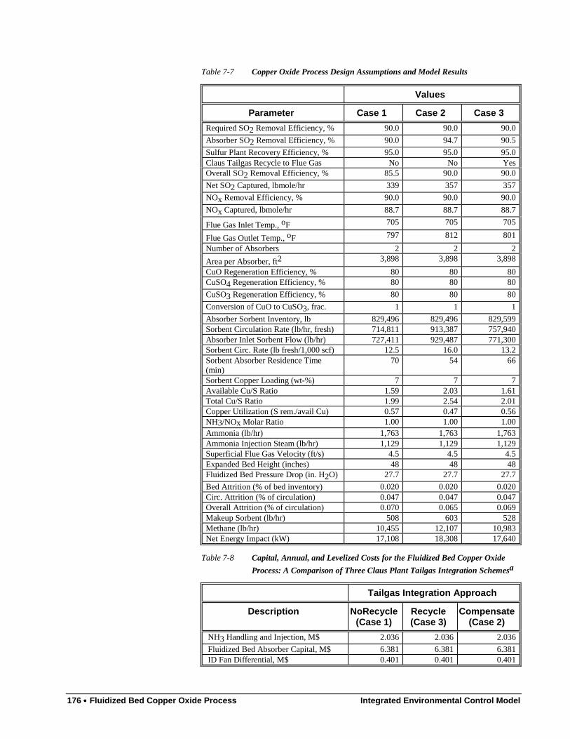
176 •••• Fluidized Bed Copper Oxide Process Integrated Environmental Control Model
Table 7-7 Copper Oxide Process Design Assumptions and Model Results
Values
Parameter Case 1 Case 2 Case 3
Required SO2 Removal Efficiency, % 90.0 90.0 90.0
Absorber SO2 Removal Efficiency, % 90.0 94.7 90.5
Sulfur Plant Recovery Efficiency, % 95.0 95.0 95.0Claus Tailgas Recycle to Flue Gas No No YesOverall SO2 Removal Efficiency, % 85.5 90.0 90.0
Net SO2 Captured, lbmole/hr 339 357 357
NOx Removal Efficiency, % 90.0 90.0 90.0
NOx Captured, lbmole/hr 88.7 88.7 88.7
Flue Gas Inlet Temp., oF 705 705 705
Flue Gas Outlet Temp., oF 797 812 801
Number of Absorbers 2 2 2
Area per Absorber, ft2 3,898 3,898 3,898
CuO Regeneration Efficiency, % 80 80 80CuSO4 Regeneration Efficiency, % 80 80 80
CuSO3 Regeneration Efficiency, % 80 80 80
Conversion of CuO to CuSO3, frac. 1 1 1
Absorber Sorbent Inventory, lb 829,496 829,496 829,599Sorbent Circulation Rate (lb/hr, fresh) 714,811 913,387 757,940Absorber Inlet Sorbent Flow (lb/hr) 727,411 929,487 771,300Sorbent Circ. Rate (lb fresh/1,000 scf) 12.5 16.0 13.2Sorbent Absorber Residence Time(min)
70 54 66
Sorbent Copper Loading (wt-%) 7 7 7Available Cu/S Ratio 1.59 2.03 1.61Total Cu/S Ratio 1.99 2.54 2.01Copper Utilization (S rem./avail Cu) 0.57 0.47 0.56NH3/NOx Molar Ratio 1.00 1.00 1.00Ammonia (lb/hr) 1,763 1,763 1,763Ammonia Injection Steam (lb/hr) 1,129 1,129 1,129Superficial Flue Gas Velocity (ft/s) 4.5 4.5 4.5Expanded Bed Height (inches) 48 48 48Fluidized Bed Pressure Drop (in. H2O) 27.7 27.7 27.7
Bed Attrition (% of bed inventory) 0.020 0.020 0.020Circ. Attrition (% of circulation) 0.047 0.047 0.047Overall Attrition (% of circulation) 0.070 0.065 0.069Makeup Sorbent (lb/hr) 508 603 528Methane (lb/hr) 10,455 12,107 10,983Net Energy Impact (kW) 17,108 18,308 17,640
Table 7-8 Capital, Annual, and Levelized Costs for the Fluidized Bed Copper Oxide
Process: A Comparison of Three Claus Plant Tailgas Integration Schemesa
Tailgas Integration Approach
Description NoRecycle(Case 1)
Recycle(Case 3)
Compensate(Case 2)
NH3 Handling and Injection, M$ 2.036 2.036 2.036
Fluidized Bed Absorber Capital, M$ 6.381 6.381 6.381 ID Fan Differential, M$ 0.401 0.401 0.401
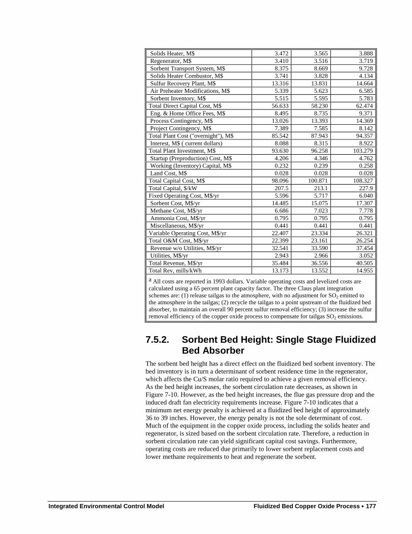
Integrated Environmental Control Model Fluidized Bed Copper Oxide Process •••• 177
Solids Heater, M$ 3.472 3.565 3.888 Regenerator, M$ 3.410 3.516 3.719 Sorbent Transport System, M$ 8.375 8.669 9.728 Solids Heater Combustor, M$ 3.741 3.828 4.134 Sulfur Recovery Plant, M$ 13.316 13.831 14.664 Air Preheater Modifications, M$ 5.339 5.623 6.585 Sorbent Inventory, M$ 5.515 5.595 5.783Total Direct Capital Cost, M$ 56.633 58.230 62.474 Eng. & Home Office Fees, M$ 8.495 8.735 9.371 Process Contingency, M$ 13.026 13.393 14.369 Project Contingency, M$ 7.389 7.585 8.142Total Plant Cost ("overnight"), M$ 85.542 87.943 94.357 Interest, M$ ( current dollars) 8.088 8.315 8.922Total Plant Investment, M$ 93.630 96.258 103.279 Startup (Preproduction) Cost, M$ 4.206 4.346 4.762 Working (Inventory) Capital, M$ 0.232 0.239 0.258 Land Cost, M$ 0.028 0.028 0.028Total Capital Cost, M$ 98.096 100.871 108.327Total Capital, $/kW 207.5 213.1 227.9Fixed Operating Cost, M$/yr 5.596 5.717 6.040 Sorbent Cost, M$/yr 14.485 15.075 17.307 Methane Cost, M$/yr 6.686 7.023 7.778 Ammonia Cost, M$/yr 0.795 0.795 0.795 Miscellaneous, M$/yr 0.441 0.441 0.441Variable Operating Cost, M$/yr 22.407 23.334 26.321Total O&M Cost, M$/yr 22.399 23.161 26.254 Revenue w/o Utilities, M$/yr 32.541 33.590 37.454 Utilities, M$/yr 2.943 2.966 3.052Total Revenue, M$/yr 35.484 36.556 40.505Total Rev, mills/kWh 13.173 13.552 14.955
a All costs are reported in 1993 dollars. Variable operating costs and levelized costs arecalculated using a 65 percent plant capacity factor. The three Claus plant integrationschemes are: (1) release tailgas to the atmosphere, with no adjustment for SO2 emitted tothe atmosphere in the tailgas; (2) recycle the tailgas to a point upstream of the fluidized bedabsorber, to maintain an overall 90 percent sulfur removal efficiency; (3) increase the sulfurremoval efficiency of the copper oxide process to compensate for tailgas SO2 emissions.
7.5.2. Sorbent Bed Height: Single Stage FluidizedBed Absorber
The sorbent bed height has a direct effect on the fluidized bed sorbent inventory. Thebed inventory is in turn a determinant of sorbent residence time in the regenerator,which affects the Cu/S molar ratio required to achieve a given removal efficiency.As the bed height increases, the sorbent circulation rate decreases, as shown inFigure 7-10. However, as the bed height increases, the flue gas pressure drop and theinduced draft fan electricity requirements increase. Figure 7-10 indicates that aminimum net energy penalty is achieved at a fluidized bed height of approximately36 to 39 inches. However, the energy penalty is not the sole determinant of cost.Much of the equipment in the copper oxide process, including the solids heater andregenerator, is sized based on the sorbent circulation rate. Therefore, a reduction insorbent circulation rate can yield significant capital cost savings. Furthermore,operating costs are reduced due primarily to lower sorbent replacement costs andlower methane requirements to heat and regenerate the sorbent.
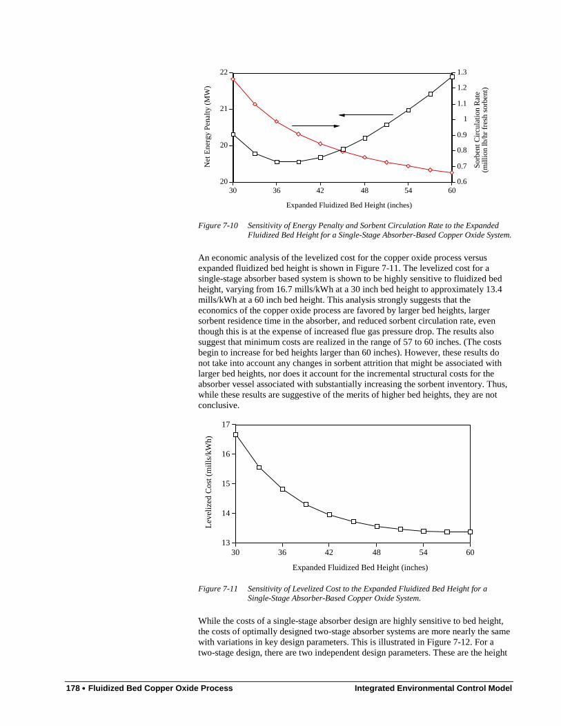
178 •••• Fluidized Bed Copper Oxide Process Integrated Environmental Control Model
0.6
0.7
0.8
0.9
1
1.1
1.2
1.3
Sor
bent
Circ
ulat
ion
Rat
e(m
illio
n lb
/hr
fres
h so
rben
t)
20
20
21
22
Net
Ene
rgy
Pen
alty
(M
W)
30 36 42 48 54 60
Expanded Fluidized Bed Height (inches)
Figure 7-10 Sensitivity of Energy Penalty and Sorbent Circulation Rate to the ExpandedFluidized Bed Height for a Single-Stage Absorber-Based Copper Oxide System.
An economic analysis of the levelized cost for the copper oxide process versusexpanded fluidized bed height is shown in Figure 7-11. The levelized cost for asingle-stage absorber based system is shown to be highly sensitive to fluidized bedheight, varying from 16.7 mills/kWh at a 30 inch bed height to approximately 13.4mills/kWh at a 60 inch bed height. This analysis strongly suggests that theeconomics of the copper oxide process are favored by larger bed heights, largersorbent residence time in the absorber, and reduced sorbent circulation rate, eventhough this is at the expense of increased flue gas pressure drop. The results alsosuggest that minimum costs are realized in the range of 57 to 60 inches. (The costsbegin to increase for bed heights larger than 60 inches). However, these results donot take into account any changes in sorbent attrition that might be associated withlarger bed heights, nor does it account for the incremental structural costs for theabsorber vessel associated with substantially increasing the sorbent inventory. Thus,while these results are suggestive of the merits of higher bed heights, they are notconclusive.
13
14
15
16
17
Leve
lized
Cos
t (m
ills/
kWh)
30 36 42 48 54 60
Expanded Fluidized Bed Height (inches)
Figure 7-11 Sensitivity of Levelized Cost to the Expanded Fluidized Bed Height for aSingle-Stage Absorber-Based Copper Oxide System.
While the costs of a single-stage absorber design are highly sensitive to bed height,the costs of optimally designed two-stage absorber systems are more nearly the samewith variations in key design parameters. This is illustrated in Figure 7-12. For atwo-stage design, there are two independent design parameters. These are the height
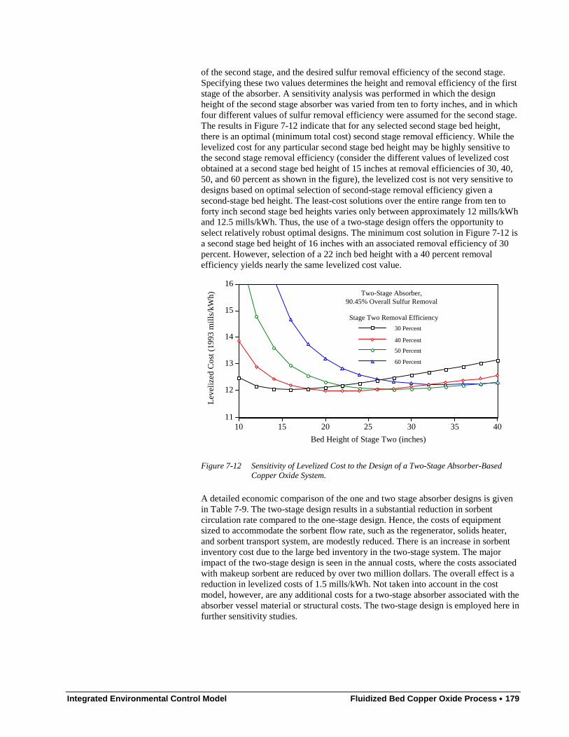
Integrated Environmental Control Model Fluidized Bed Copper Oxide Process •••• 179
of the second stage, and the desired sulfur removal efficiency of the second stage.Specifying these two values determines the height and removal efficiency of the firststage of the absorber. A sensitivity analysis was performed in which the designheight of the second stage absorber was varied from ten to forty inches, and in whichfour different values of sulfur removal efficiency were assumed for the second stage.The results in Figure 7-12 indicate that for any selected second stage bed height,there is an optimal (minimum total cost) second stage removal efficiency. While thelevelized cost for any particular second stage bed height may be highly sensitive tothe second stage removal efficiency (consider the different values of levelized costobtained at a second stage bed height of 15 inches at removal efficiencies of 30, 40,50, and 60 percent as shown in the figure), the levelized cost is not very sensitive todesigns based on optimal selection of second-stage removal efficiency given asecond-stage bed height. The least-cost solutions over the entire range from ten toforty inch second stage bed heights varies only between approximately 12 mills/kWhand 12.5 mills/kWh. Thus, the use of a two-stage design offers the opportunity toselect relatively robust optimal designs. The minimum cost solution in Figure 7-12 isa second stage bed height of 16 inches with an associated removal efficiency of 30percent. However, selection of a 22 inch bed height with a 40 percent removalefficiency yields nearly the same levelized cost value.
11
12
13
14
15
16
Le
veliz
ed
Co
st (
19
93
mill
s/kW
h)
10 15 20 25 30 35 40
Bed Height of Stage Two (inches)
60 Percent
50 Percent
40 Percent
30 Percent
Stage Two Removal Efficiency
Two-Stage Absorber,90.45% Overall Sulfur Removal
Figure 7-12 Sensitivity of Levelized Cost to the Design of a Two-Stage Absorber-BasedCopper Oxide System.
A detailed economic comparison of the one and two stage absorber designs is givenin Table 7-9. The two-stage design results in a substantial reduction in sorbentcirculation rate compared to the one-stage design. Hence, the costs of equipmentsized to accommodate the sorbent flow rate, such as the regenerator, solids heater,and sorbent transport system, are modestly reduced. There is an increase in sorbentinventory cost due to the large bed inventory in the two-stage system. The majorimpact of the two-stage design is seen in the annual costs, where the costs associatedwith makeup sorbent are reduced by over two million dollars. The overall effect is areduction in levelized costs of 1.5 mills/kWh. Not taken into account in the costmodel, however, are any additional costs for a two-stage absorber associated with theabsorber vessel material or structural costs. The two-stage design is employed here infurther sensitivity studies.
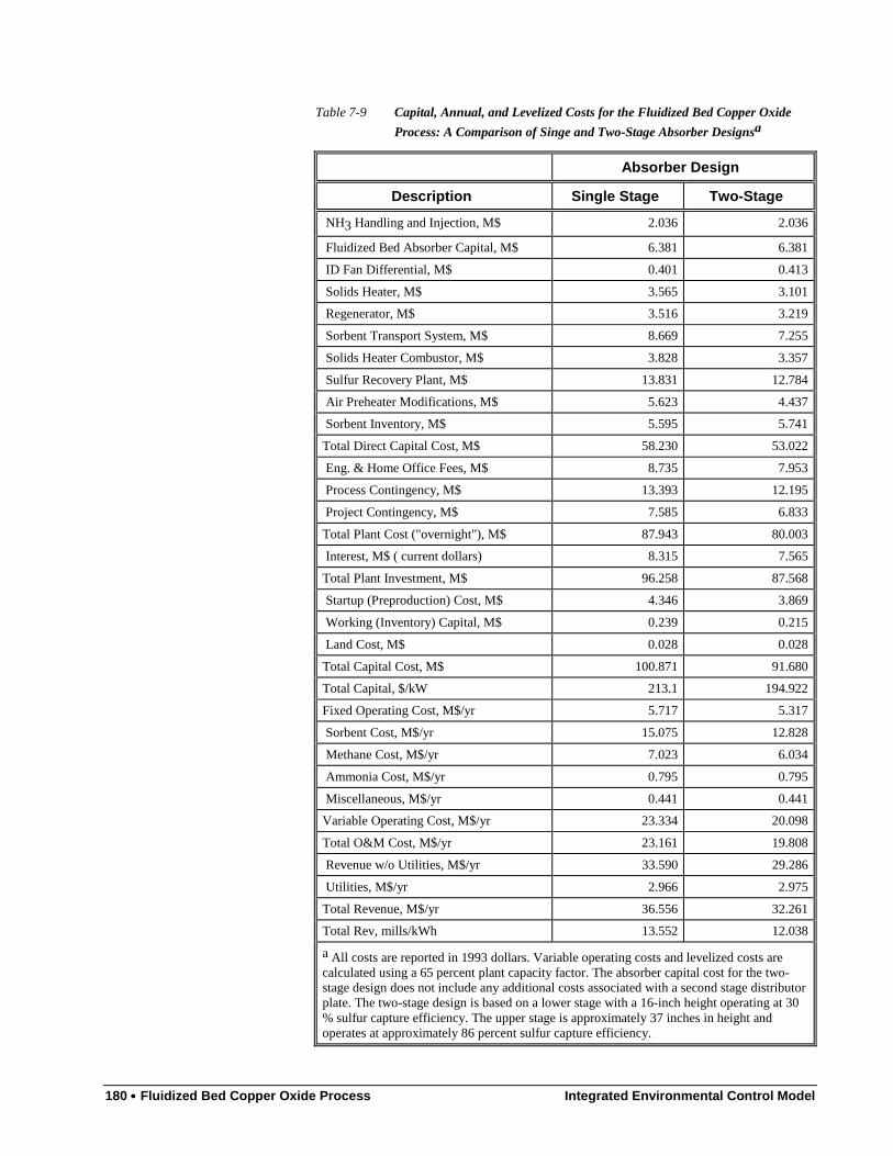
180 •••• Fluidized Bed Copper Oxide Process Integrated Environmental Control Model
Table 7-9 Capital, Annual, and Levelized Costs for the Fluidized Bed Copper Oxide
Process: A Comparison of Singe and Two-Stage Absorber Designsa
Absorber Design
Description Single Stage Two-Stage
NH3 Handling and Injection, M$ 2.036 2.036
Fluidized Bed Absorber Capital, M$ 6.381 6.381
ID Fan Differential, M$ 0.401 0.413
Solids Heater, M$ 3.565 3.101
Regenerator, M$ 3.516 3.219
Sorbent Transport System, M$ 8.669 7.255
Solids Heater Combustor, M$ 3.828 3.357
Sulfur Recovery Plant, M$ 13.831 12.784
Air Preheater Modifications, M$ 5.623 4.437
Sorbent Inventory, M$ 5.595 5.741
Total Direct Capital Cost, M$ 58.230 53.022
Eng. & Home Office Fees, M$ 8.735 7.953
Process Contingency, M$ 13.393 12.195
Project Contingency, M$ 7.585 6.833
Total Plant Cost ("overnight"), M$ 87.943 80.003
Interest, M$ ( current dollars) 8.315 7.565
Total Plant Investment, M$ 96.258 87.568
Startup (Preproduction) Cost, M$ 4.346 3.869
Working (Inventory) Capital, M$ 0.239 0.215
Land Cost, M$ 0.028 0.028
Total Capital Cost, M$ 100.871 91.680
Total Capital, $/kW 213.1 194.922
Fixed Operating Cost, M$/yr 5.717 5.317
Sorbent Cost, M$/yr 15.075 12.828
Methane Cost, M$/yr 7.023 6.034
Ammonia Cost, M$/yr 0.795 0.795
Miscellaneous, M$/yr 0.441 0.441
Variable Operating Cost, M$/yr 23.334 20.098
Total O&M Cost, M$/yr 23.161 19.808
Revenue w/o Utilities, M$/yr 33.590 29.286
Utilities, M$/yr 2.966 2.975
Total Revenue, M$/yr 36.556 32.261
Total Rev, mills/kWh 13.552 12.038
a All costs are reported in 1993 dollars. Variable operating costs and levelized costs arecalculated using a 65 percent plant capacity factor. The absorber capital cost for the two-stage design does not include any additional costs associated with a second stage distributorplate. The two-stage design is based on a lower stage with a 16-inch height operating at 30% sulfur capture efficiency. The upper stage is approximately 37 inches in height andoperates at approximately 86 percent sulfur capture efficiency.
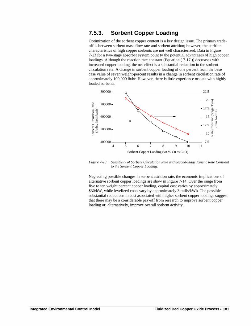
Integrated Environmental Control Model Fluidized Bed Copper Oxide Process •••• 181
7.5.3. Sorbent Copper LoadingOptimization of the sorbent copper content is a key design issue. The primary trade-off is between sorbent mass flow rate and sorbent attrition; however, the attritioncharacteristics of high copper sorbents are not well characterized. Data in Figure7-13 for a two-stage absorber system point to the potential advantages of high copperloadings. Although the reaction rate constant (Equation ( 7-17 )) decreases withincreased copper loading, the net effect is a substantial reduction in the sorbentcirculation rate. A change in sorbent copper loading of one percent from the basecase value of seven weight-percent results in a change in sorbent circulation rate ofapproximately 100,000 lb/hr. However, there is little experience or data with highlyloaded sorbents.
7.5
10
12.5
15
17.5
20
22.5
Rat
e C
onst
ant (
Sta
ge T
wo)
(min
-1-a
tm-1
)
400000
500000
600000
700000
800000S
orbe
nt C
ircul
atio
n R
ate
(lb/h
r, fr
esh
basi
s)
4 5 6 7 8 9 10 11
Sorbent Copper Loading (wt-% Cu as CuO)
Figure 7-13 Sensitivity of Sorbent Circulation Rate and Second-Stage Kinetic Rate Constantto the Sorbent Copper Loading.
Neglecting possible changes in sorbent attrition rate, the economic implications ofalternative sorbent copper loadings are show in Figure 7-14. Over the range fromfive to ten weight percent copper loading, capital cost varies by approximately$30/kW, while levelized costs vary by approximately 3 mills/kWh. The possiblesubstantial reductions in cost associated with higher sorbent copper loadings suggestthat there may be a considerable pay-off from research to improve sorbent copperloading or, alternatively, improve overall sorbent activity.
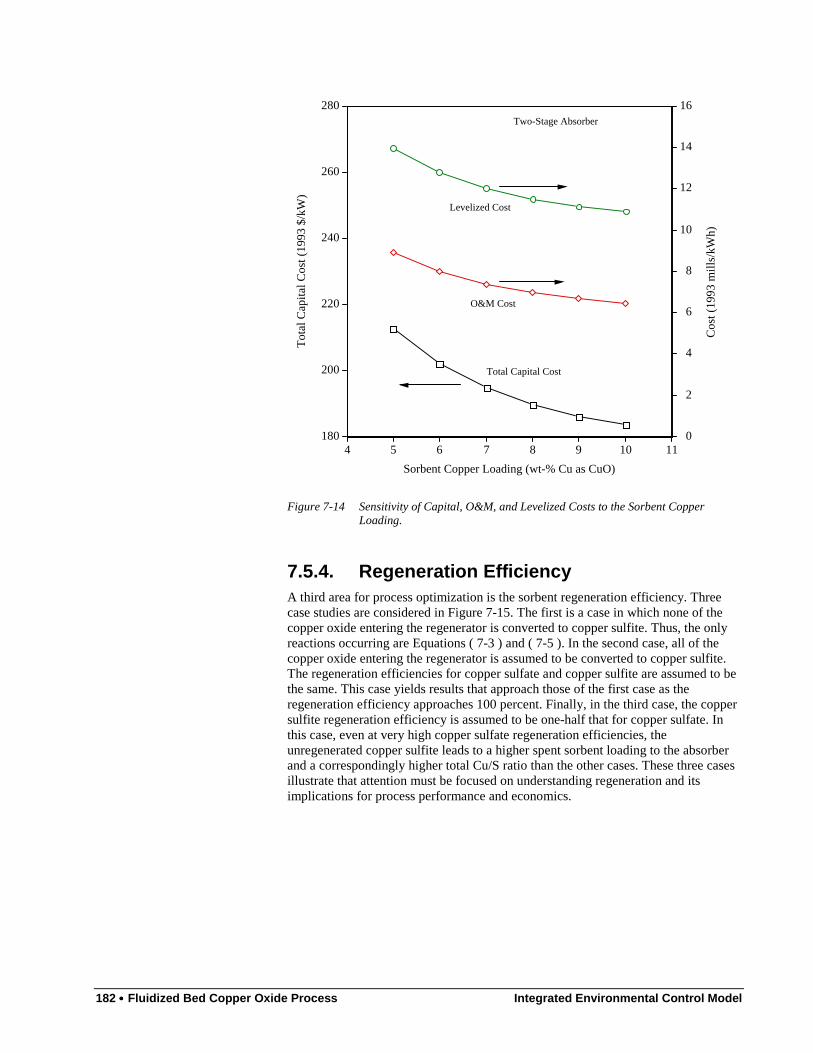
182 •••• Fluidized Bed Copper Oxide Process Integrated Environmental Control Model
0
2
4
6
8
10
12
14
16
Co
st (
19
93
mill
s/kW
h)
180
200
220
240
260
280
To
tal C
ap
ital C
ost
(1
99
3 $
/kW
)
4 5 6 7 8 9 10 11
Sorbent Copper Loading (wt-% Cu as CuO)
Total Capital Cost
Levelized Cost
O&M Cost
Two-Stage Absorber
Figure 7-14 Sensitivity of Capital, O&M, and Levelized Costs to the Sorbent CopperLoading.
7.5.4. Regeneration EfficiencyA third area for process optimization is the sorbent regeneration efficiency. Threecase studies are considered in Figure 7-15. The first is a case in which none of thecopper oxide entering the regenerator is converted to copper sulfite. Thus, the onlyreactions occurring are Equations ( 7-3 ) and ( 7-5 ). In the second case, all of thecopper oxide entering the regenerator is assumed to be converted to copper sulfite.The regeneration efficiencies for copper sulfate and copper sulfite are assumed to bethe same. This case yields results that approach those of the first case as theregeneration efficiency approaches 100 percent. Finally, in the third case, the coppersulfite regeneration efficiency is assumed to be one-half that for copper sulfate. Inthis case, even at very high copper sulfate regeneration efficiencies, theunregenerated copper sulfite leads to a higher spent sorbent loading to the absorberand a correspondingly higher total Cu/S ratio than the other cases. These three casesillustrate that attention must be focused on understanding regeneration and itsimplications for process performance and economics.

Integrated Environmental Control Model Fluidized Bed Copper Oxide Process •••• 183
0
1
2
3
4
5
To
tal C
u/S
Ra
tio
0
1
2
3
4
5
To
tal C
u/S
Ra
tio0.40 0.50 0.60 0.70 0.80 0.90 1.00
Regeneration Efficiency for CuO and CuSO4
Plus CuSO3 Regenerated at Only Half the
Efficiency of CuO and CuSO4
All CuO forms CuSO3
No CuSO3 Formed in Regenerator
Results are for a Two-Stage Absorber Design
Figure 7-15 Sensitivity of the Total Cu/S Molar Ratio to Regeneration Efficiencies.
The economic implications of poor regeneration are shown in Figure 7-16. At lowregeneration efficiencies, typical of those believed to have occurred in life cycletesting, the levelized costs may be as much as double or more the costs based on basecase assumptions of 80 percent regeneration.
10
15
20
25
30
Le
veliz
ed
Co
st (
19
93
mill
s/kW
h)
10
15
20
25
30
Le
veliz
ed
Co
st (
19
93
mill
s/kW
h)
0.40 0.50 0.60 0.70 0.80 0.90 1.00
Regeneration Efficiency for CuO and CuSO4
Plus CuSO3 Regenerated at Only Half the
Efficiency of CuO and CuSO4
No CuSO3 Formed in Regenerator
All CuO forms CuSO3
Results are for a Two-Stage Absorber Design
Figure 7-16 Sensitivity of Levelized Cost to Regeneration Efficiencies.
7.5.5. Regenerator Inlet TemperatureThe regenerator sorbent residence required to achieve a given regeneration efficiencyis a function of the temperature of the inlet sorbent. This sensitivity is shown inFigure 7-17, together with a sensitivity analysis for the total methane required for thecopper oxide process. As the sorbent inlet temperature is reduced, the kinetics of theregeneration reactions slow, leading to a requirement for a longer sorbent residencetime to achieve a given copper sulfate conversion efficiency to copper. Astemperature is reduced, however, less methane is required in the solids heatercombustor to provide hot gases for sorbent heating.
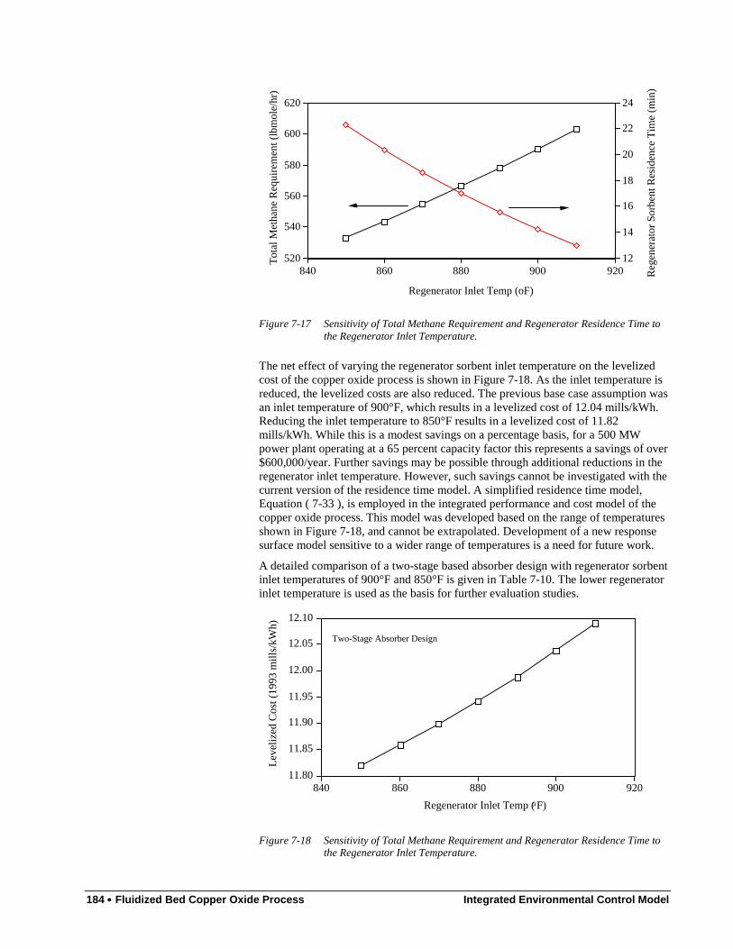
184 •••• Fluidized Bed Copper Oxide Process Integrated Environmental Control Model
12
14
16
18
20
22
24
Reg
ener
ator
Sor
bent
Res
iden
ce T
ime
(min
)
520
540
560
580
600
620
Tot
al M
etha
ne R
equi
rem
ent
(lbm
ole/
hr)
840 860 880 900 920
Regenerator Inlet Temp (oF)
Figure 7-17 Sensitivity of Total Methane Requirement and Regenerator Residence Time tothe Regenerator Inlet Temperature.
The net effect of varying the regenerator sorbent inlet temperature on the levelizedcost of the copper oxide process is shown in Figure 7-18. As the inlet temperature isreduced, the levelized costs are also reduced. The previous base case assumption wasan inlet temperature of 900°F, which results in a levelized cost of 12.04 mills/kWh.Reducing the inlet temperature to 850°F results in a levelized cost of 11.82mills/kWh. While this is a modest savings on a percentage basis, for a 500 MWpower plant operating at a 65 percent capacity factor this represents a savings of over$600,000/year. Further savings may be possible through additional reductions in theregenerator inlet temperature. However, such savings cannot be investigated with thecurrent version of the residence time model. A simplified residence time model,Equation ( 7-33 ), is employed in the integrated performance and cost model of thecopper oxide process. This model was developed based on the range of temperaturesshown in Figure 7-18, and cannot be extrapolated. Development of a new responsesurface model sensitive to a wider range of temperatures is a need for future work.
A detailed comparison of a two-stage based absorber design with regenerator sorbentinlet temperatures of 900°F and 850°F is given in Table 7-10. The lower regeneratorinlet temperature is used as the basis for further evaluation studies.
11.80
11.85
11.90
11.95
12.00
12.05
12.10
Leve
lized
Cos
t (19
93 m
ills/
kWh)
840 860 880 900 920
Regenerator Inlet Temp (oF)
Two-Stage Absorber Design
Figure 7-18 Sensitivity of Total Methane Requirement and Regenerator Residence Time tothe Regenerator Inlet Temperature.

Integrated Environmental Control Model Fluidized Bed Copper Oxide Process •••• 185
Table 7-10 Capital, Annual, and Levelized Costs for the Fluidized Bed Copper Oxide
Process: Effect of Regeneration Temperature on Costsa
Regenerator Temperature
Description 900oF 850oF
NH3 Handling and Injection, M$ 2.036 2.036 Fluidized Bed Absorber Capital, M$ 6.381 6.381 ID Fan Differential, M$ 0.413 0.414 Solids Heater, M$ 3.101 2.756 Regenerator, M$ 3.219 3.540 Sorbent Transport System, M$ 7.255 7.258 Solids Heater Combustor, M$ 3.357 2.668 Sulfur Recovery Plant, M$ 12.784 12.785 Air Preheater Modifications, M$ 4.437 3.784 Sorbent Inventory, M$ 5.741 6.170Total Direct Capital Cost, M$ 53.022 51.956 Eng. & Home Office Fees, M$ 7.953 7.793 Process Contingency, M$ 12.195 11.950 Project Contingency, M$ 6.833 6.626Total Plant Cost ("overnight"), M$ 80.003 78.326 Interest, M$ ( current dollars) 7.565 7.406Total Plant Investment, M$ 87.568 85.732 Startup (Preproduction) Cost, M$ 3.869 3.782 Working (Inventory) Capital, M$ 0.215 0.208 Land Cost, M$ 0.028 0.028Total Capital Cost, M$ 91.680 89.749Total Capital, $/kW 194.922 191.428Fixed Operating Cost, M$/yr 5.317 5.232 Sorbent Cost, M$/yr 12.828 12.884 Methane Cost, M$/yr 6.034 5.451 Ammonia Cost, M$/yr 0.795 0.795 Miscellaneous, M$/yr 0.441 0.441Variable Operating Cost, M$/yr 20.098 19.571Total O&M Cost, M$/yr 19.808 19.345 Revenue w/o Utilities, M$/yr 29.286 28.624 Utilities, M$/yr 2.975 2.954Total Revenue, M$/yr 32.261 31.578Total Rev, mills/kWh 12.038 11.821
a All costs are reported in 1993 dollars. Variable operating costs and levelized costs arecalculated using a 65 percent plant capacity factor. The absorber capital cost for the two-stage design does not include any additional costs associated with a second stage distributorplate. The two-stage design is based on a lower stage with a 16-inch height operating at 30% sulfur capture efficiency. The upper stage is approximately 37 inches in height andoperates at approximately 86 percent sulfur capture efficiency. The first case is for aregenerator sorbent inlet temperature of 900°F. The second case is for a regenerator sorbentinlet temperature of 850°F.
7.6. Probabilistic AnalysisA probabilistic analysis was performed to evaluate uncertainties in the copper oxideprocess. This technology has been tested on only a small-scale, with no large-scalecommercial experience that is required to verify expectations of performance andcost. Therefore, any estimate of performance or cost for this technology is subject touncertainty.
186 •••• Fluidized Bed Copper Oxide Process Integrated Environmental Control Model
A probabilistic analysis requires input assumptions or data regarding theuncertainties in key process and economic parameters. There are several types ofuncertainty in trying to predict the commercial-scale performance and cost of a newprocess technology. These include statistical error, systematic error, variability, andlack of an empirical basis for concepts that have not been tested. Uncertainties mayapply to different aspects of the process, including performance variables, equipmentsizing parameters, process area capital costs, requirements for initial catalysts andchemicals, indirect capital costs, process area maintenance costs, requirements forconsumables during plant operation, and the unit costs of consumables, byproducts,wastes, and fuel. Model parameters in any or all of these areas may be uncertain,depending on the state of development of the technology, the level of detail of theperformance and cost estimates, and future market conditions for new chemicals,catalysts, byproducts, wastes, and other process components.
It may not always be possible to develop estimates of uncertainty based on classicalstatistical analysis, nor would such an approach be appropriate in many cases.Particularly for new process technologies, data may be lacking regarding some typesof uncertainty. For example, the effect of scale-up on process performance may notbe fully understood. Thus, analysis of bench-scale test data alone may be aninsufficient basis for estimating the total uncertainty in a variable. When data arelacking, estimates of uncertainty must rely on the informed judgments of technicalexperts. Judgments regarding uncertainties can be encoded as probabilitydistributions, using techniques discussed elsewhere (see Appendix A for anoverview).
7.6.1. Input Uncertainty AssumptionsUncertainties in specific performance and cost parameters were explicitlycharacterized using probability distributions. Identification of parameters that shouldbe treated probabilistically, and the estimates of uncertainties for these parameters,were based on literature review, data analysis, and elicitation of expert judgmentsfrom USDOE FETC process engineers involved in technology development. Thisapproach has also been applied by Frey et al. (1994) for evaluating an integratedgasification combined cycle (IGCC) system.
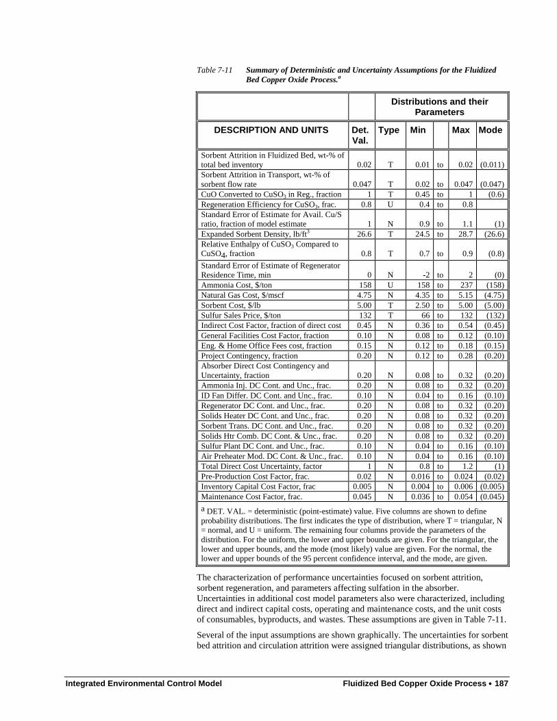
Integrated Environmental Control Model Fluidized Bed Copper Oxide Process •••• 187
Table 7-11 Summary of Deterministic and Uncertainty Assumptions for the FluidizedBed Copper Oxide Process.a
Distributions and theirParameters
DESCRIPTION AND UNITS Det.Val.
Type Min Max Mode
Sorbent Attrition in Fluidized Bed, wt-% oftotal bed inventory 0.02 T 0.01 to 0.02 (0.011)Sorbent Attrition in Transport, wt-% ofsorbent flow rate 0.047 T 0.02 to 0.047 (0.047)CuO Converted to CuSO3 in Reg., fraction 1 T 0.45 to 1 (0.6)Regeneration Efficiency for CuSO3, frac. 0.8 U 0.4 to 0.8Standard Error of Estimate for Avail. Cu/Sratio, fraction of model estimate 1 N 0.9 to 1.1 (1)Expanded Sorbent Density, lb/ft3 26.6 T 24.5 to 28.7 (26.6)Relative Enthalpy of CuSO3 Compared toCuSO4, fraction 0.8 T 0.7 to 0.9 (0.8)
Standard Error of Estimate of RegeneratorResidence Time, min 0 N -2 to 2 (0)Ammonia Cost, $/ton 158 U 158 to 237 (158)Natural Gas Cost, $/mscf 4.75 N 4.35 to 5.15 (4.75)Sorbent Cost, $/lb 5.00 T 2.50 to 5.00 (5.00)Sulfur Sales Price, $/ton 132 T 66 to 132 (132)Indirect Cost Factor, fraction of direct cost 0.45 N 0.36 to 0.54 (0.45)General Facilities Cost Factor, fraction 0.10 N 0.08 to 0.12 (0.10)Eng. & Home Office Fees cost, fraction 0.15 N 0.12 to 0.18 (0.15)Project Contingency, fraction 0.20 N 0.12 to 0.28 (0.20)Absorber Direct Cost Contingency andUncertainty, fraction 0.20 N 0.08 to 0.32 (0.20)Ammonia Inj. DC Cont. and Unc., frac. 0.20 N 0.08 to 0.32 (0.20)ID Fan Differ. DC Cont. and Unc., frac. 0.10 N 0.04 to 0.16 (0.10)Regenerator DC Cont. and Unc., frac. 0.20 N 0.08 to 0.32 (0.20)Solids Heater DC Cont. and Unc., frac. 0.20 N 0.08 to 0.32 (0.20)Sorbent Trans. DC Cont. and Unc., frac. 0.20 N 0.08 to 0.32 (0.20)Solids Htr Comb. DC Cont. & Unc., frac. 0.20 N 0.08 to 0.32 (0.20)Sulfur Plant DC Cont. and Unc., frac. 0.10 N 0.04 to 0.16 (0.10)Air Preheater Mod. DC Cont. & Unc., frac. 0.10 N 0.04 to 0.16 (0.10)Total Direct Cost Uncertainty, factor 1 N 0.8 to 1.2 (1)Pre-Production Cost Factor, frac. 0.02 N 0.016 to 0.024 (0.02)Inventory Capital Cost Factor, frac 0.005 N 0.004 to 0.006 (0.005)Maintenance Cost Factor, frac. 0.045 N 0.036 to 0.054 (0.045)
a DET. VAL. = deterministic (point-estimate) value. Five columns are shown to defineprobability distributions. The first indicates the type of distribution, where T = triangular, N= normal, and U = uniform. The remaining four columns provide the parameters of thedistribution. For the uniform, the lower and upper bounds are given. For the triangular, thelower and upper bounds, and the mode (most likely) value are given. For the normal, thelower and upper bounds of the 95 percent confidence interval, and the mode, are given.
The characterization of performance uncertainties focused on sorbent attrition,sorbent regeneration, and parameters affecting sulfation in the absorber.Uncertainties in additional cost model parameters also were characterized, includingdirect and indirect capital costs, operating and maintenance costs, and the unit costsof consumables, byproducts, and wastes. These assumptions are given in Table 7-11.
Several of the input assumptions are shown graphically. The uncertainties for sorbentbed attrition and circulation attrition were assigned triangular distributions, as shown
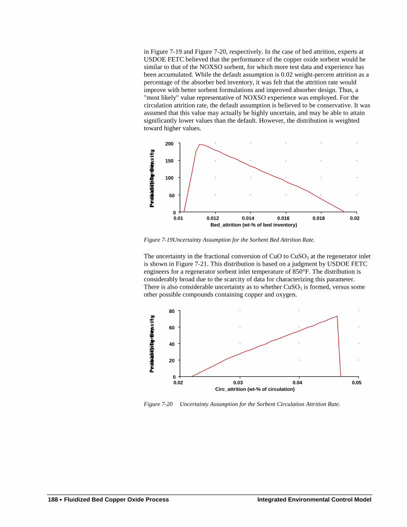
188 •••• Fluidized Bed Copper Oxide Process Integrated Environmental Control Model
in Figure 7-19 and Figure 7-20, respectively. In the case of bed attrition, experts atUSDOE FETC believed that the performance of the copper oxide sorbent would besimilar to that of the NOXSO sorbent, for which more test data and experience hasbeen accumulated. While the default assumption is 0.02 weight-percent attrition as apercentage of the absorber bed inventory, it was felt that the attrition rate wouldimprove with better sorbent formulations and improved absorber design. Thus, a"most likely" value representative of NOXSO experience was employed. For thecirculation attrition rate, the default assumption is believed to be conservative. It wasassumed that this value may actually be highly uncertain, and may be able to attainsignificantly lower values than the default. However, the distribution is weightedtoward higher values.
Pro
babi
lity
Den
sity
Bed_attrition (wt-% of bed inventory)0.01 0.012 0.014 0.016 0.018 0.020
50
100
150
200
Figure 7-19Uncertainty Assumption for the Sorbent Bed Attrition Rate.
The uncertainty in the fractional conversion of CuO to CuSO3 at the regenerator inletis shown in Figure 7-21. This distribution is based on a judgment by USDOE FETCengineers for a regenerator sorbent inlet temperature of 850°F. The distribution isconsiderably broad due to the scarcity of data for characterizing this parameter.There is also considerable uncertainty as to whether CuSO3 is formed, versus someother possible compounds containing copper and oxygen.
Pro
babi
lity
Den
sity
Circ_attrition (wt-% of circulation)0.02 0.03 0.04 0.050
20
40
60
80
Figure 7-20 Uncertainty Assumption for the Sorbent Circulation Attrition Rate.

Integrated Environmental Control Model Fluidized Bed Copper Oxide Process •••• 189
Pro
babi
lity
Den
sity
X1 (fraction)0.4 0.6 0.8 1
0
1
2
3
4
Figure 7-21 Uncertainty Assumption for the Fractional Conversion of CuO to CuSO3 at the
Regenerator Inlet.
The uncertainty in the regeneration efficiency for CuSO3 is characterized as uniformdistribution (see Figure 7-22), based on a judgment by USDOE FETC personnel.The lower end of the range represents a tentative observation in some preliminaryexperimental work on the kinetics of copper oxide sorbent regeneration. The upperend represents expectations for the regeneration of copper sulfate in a commercialscale regenerator.
The sorbent expanded density has exhibited considerable variability in previousexperimental work. This variability is represented by the triangular distributionshown in Figure 7-23.
The uncertainty in sorbent unit cost is shown in Figure 7-24. USDOE FETCpersonnel believe that the sorbent cost will be reduced from its nominal value of$5/lb with commercialization of the technology and mass production of the sorbent.
Pro
babi
lity
Den
sity
Hr1 (fraction)0.4 0.5 0.6 0.7 0.8
0
0.5
1
1.5
2
2.5
Figure 7-22 Uncertainty Assumption for the Regeneration Efficiency of CuSO3.
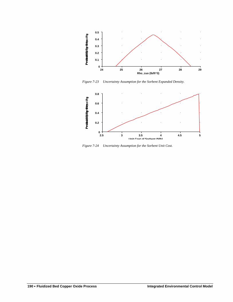
190 •••• Fluidized Bed Copper Oxide Process Integrated Environmental Control Model
Pro
babi
lity
Den
sity
Rho_cuo (lb/ft^3)24 25 26 27 28 29
0
0.1
0.2
0.3
0.4
0.5
Figure 7-23 Uncertainty Assumption for the Sorbent Expanded Density.
Pro
babi
lity
Den
sity
Unit Cost of Sorbent ($/lb)2.5 3 3.5 4 4.5 5
0
0.2
0.4
0.6
0.8
Figure 7-24 Uncertainty Assumption for the Sorbent Unit Cost.
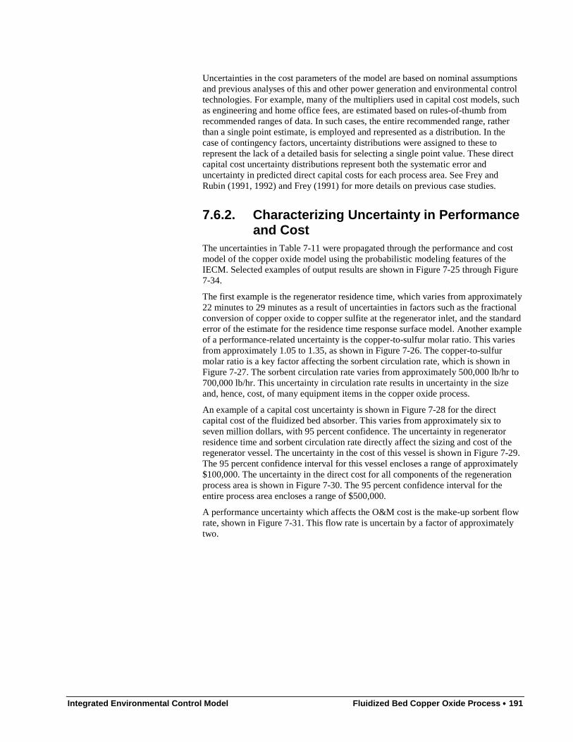
Integrated Environmental Control Model Fluidized Bed Copper Oxide Process •••• 191
Uncertainties in the cost parameters of the model are based on nominal assumptionsand previous analyses of this and other power generation and environmental controltechnologies. For example, many of the multipliers used in capital cost models, suchas engineering and home office fees, are estimated based on rules-of-thumb fromrecommended ranges of data. In such cases, the entire recommended range, ratherthan a single point estimate, is employed and represented as a distribution. In thecase of contingency factors, uncertainty distributions were assigned to these torepresent the lack of a detailed basis for selecting a single point value. These directcapital cost uncertainty distributions represent both the systematic error anduncertainty in predicted direct capital costs for each process area. See Frey andRubin (1991, 1992) and Frey (1991) for more details on previous case studies.
7.6.2. Characterizing Uncertainty in Performanceand Cost
The uncertainties in Table 7-11 were propagated through the performance and costmodel of the copper oxide model using the probabilistic modeling features of theIECM. Selected examples of output results are shown in Figure 7-25 through Figure7-34.
The first example is the regenerator residence time, which varies from approximately22 minutes to 29 minutes as a result of uncertainties in factors such as the fractionalconversion of copper oxide to copper sulfite at the regenerator inlet, and the standarderror of the estimate for the residence time response surface model. Another exampleof a performance-related uncertainty is the copper-to-sulfur molar ratio. This variesfrom approximately 1.05 to 1.35, as shown in Figure 7-26. The copper-to-sulfurmolar ratio is a key factor affecting the sorbent circulation rate, which is shown inFigure 7-27. The sorbent circulation rate varies from approximately 500,000 lb/hr to700,000 lb/hr. This uncertainty in circulation rate results in uncertainty in the sizeand, hence, cost, of many equipment items in the copper oxide process.
An example of a capital cost uncertainty is shown in Figure 7-28 for the directcapital cost of the fluidized bed absorber. This varies from approximately six toseven million dollars, with 95 percent confidence. The uncertainty in regeneratorresidence time and sorbent circulation rate directly affect the sizing and cost of theregenerator vessel. The uncertainty in the cost of this vessel is shown in Figure 7-29.The 95 percent confidence interval for this vessel encloses a range of approximately$100,000. The uncertainty in the direct cost for all components of the regenerationprocess area is shown in Figure 7-30. The 95 percent confidence interval for theentire process area encloses a range of $500,000.
A performance uncertainty which affects the O&M cost is the make-up sorbent flowrate, shown in Figure 7-31. This flow rate is uncertain by a factor of approximatelytwo.

192 •••• Fluidized Bed Copper Oxide Process Integrated Environmental Control Model
Cum
ulat
ive
Pro
babi
lity
Regenerator Residence Time (min)20 22 24 26 28 30
0
0.2
0.4
0.6
0.8
1
Figure 7-25 Uncertainty Result for Regenerator Residence Time.
Cum
ulat
ive
Pro
babi
lity
Available Cu/S Molar Ratio (lbmole CuO/lbmole SOx)1 1.1 1.2 1.3 1.4
0
0.2
0.4
0.6
0.8
1
Figure 7-26 Uncertainty Result for Available Copper-to-Sulfur Molar Ratio.
Cum
ulat
ive
Pro
babi
lity
Msorbfresh (lb/hr)450K 500K 550K 600K 650K 700K0
0.2
0.4
0.6
0.8
1
Figure 7-27 Uncertainty Result for Sorbent Circulation Rate (on a Fresh Basis).
Cum
ulat
ive
Pro
babi
lity
DCC Absorber ($M)5.75 6 6.25 6.5 6.75 70
0.2
0.4
0.6
0.8
1
Figure 7-28 Uncertainty Result for the Direct Cost of the Absorber Process Area.
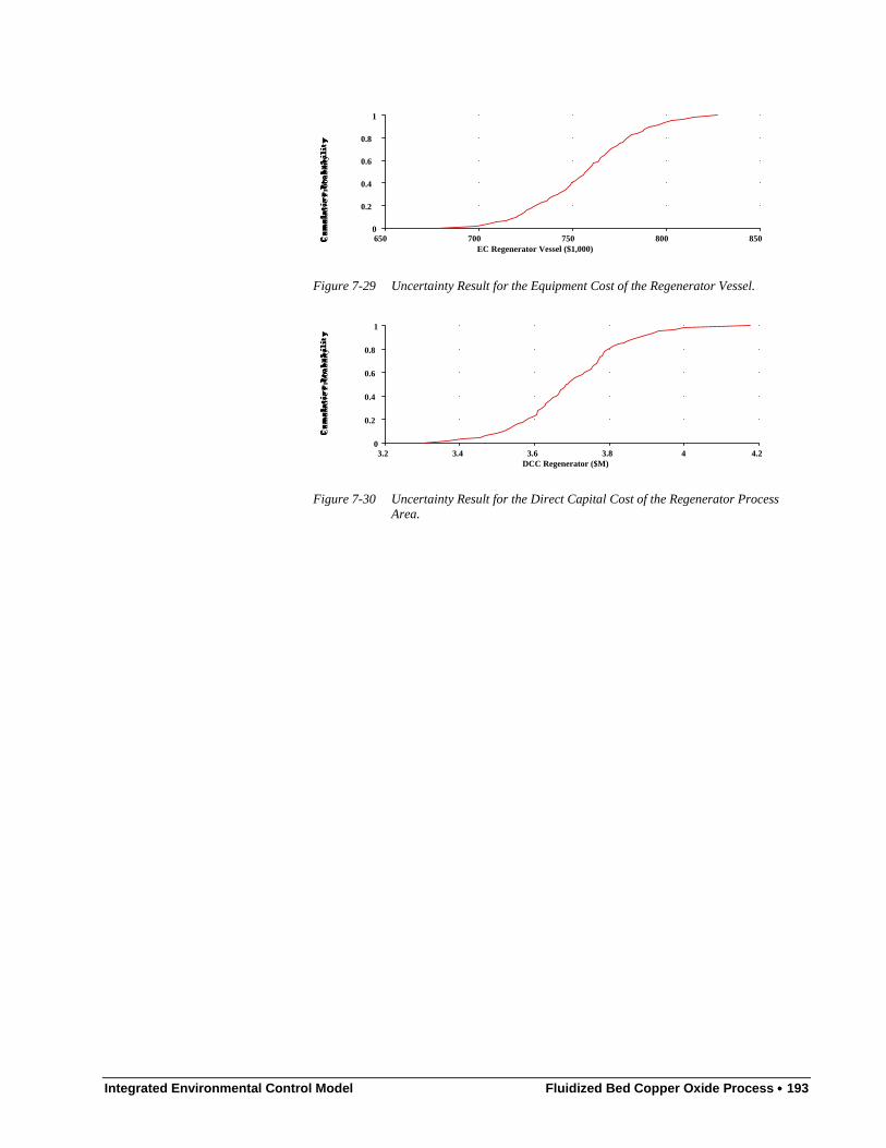
Integrated Environmental Control Model Fluidized Bed Copper Oxide Process •••• 193
Cum
ulat
ive
Pro
babi
lity
EC Regenerator Vessel ($1,000)650 700 750 800 8500
0.2
0.4
0.6
0.8
1
Figure 7-29 Uncertainty Result for the Equipment Cost of the Regenerator Vessel.
Cum
ulat
ive
Pro
babi
lity
DCC Regenerator ($M)3.2 3.4 3.6 3.8 4 4.2
0
0.2
0.4
0.6
0.8
1
Figure 7-30 Uncertainty Result for the Direct Capital Cost of the Regenerator ProcessArea.
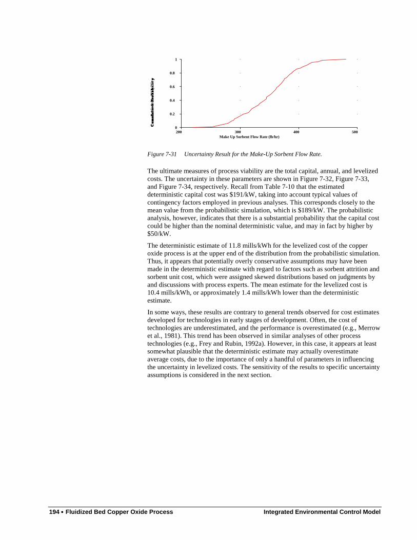
194 •••• Fluidized Bed Copper Oxide Process Integrated Environmental Control Model
Cum
ulat
ive
Pro
babi
lity
Make Up Sorbent Flow Rate (lb/hr)200 300 400 5000
0.2
0.4
0.6
0.8
1
Figure 7-31 Uncertainty Result for the Make-Up Sorbent Flow Rate.
The ultimate measures of process viability are the total capital, annual, and levelizedcosts. The uncertainty in these parameters are shown in Figure 7-32, Figure 7-33,and Figure 7-34, respectively. Recall from Table 7-10 that the estimateddeterministic capital cost was $191/kW, taking into account typical values ofcontingency factors employed in previous analyses. This corresponds closely to themean value from the probabilistic simulation, which is $189/kW. The probabilisticanalysis, however, indicates that there is a substantial probability that the capital costcould be higher than the nominal deterministic value, and may in fact by higher by$50/kW.
The deterministic estimate of 11.8 mills/kWh for the levelized cost of the copperoxide process is at the upper end of the distribution from the probabilistic simulation.Thus, it appears that potentially overly conservative assumptions may have beenmade in the deterministic estimate with regard to factors such as sorbent attrition andsorbent unit cost, which were assigned skewed distributions based on judgments byand discussions with process experts. The mean estimate for the levelized cost is10.4 mills/kWh, or approximately 1.4 mills/kWh lower than the deterministicestimate.
In some ways, these results are contrary to general trends observed for cost estimatesdeveloped for technologies in early stages of development. Often, the cost oftechnologies are underestimated, and the performance is overestimated (e.g., Merrowet al., 1981). This trend has been observed in similar analyses of other processtechnologies (e.g., Frey and Rubin, 1992a). However, in this case, it appears at leastsomewhat plausible that the deterministic estimate may actually overestimateaverage costs, due to the importance of only a handful of parameters in influencingthe uncertainty in levelized costs. The sensitivity of the results to specific uncertaintyassumptions is considered in the next section.
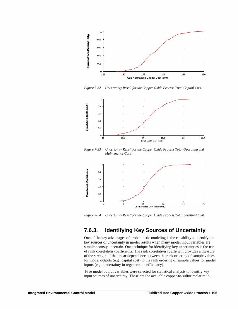
Integrated Environmental Control Model Fluidized Bed Copper Oxide Process •••• 195
Cum
ulat
ive
Pro
babi
lity
Cuo Normalized Capital Cost ($/kW)125 150 175 200 225 250
0
0.2
0.4
0.6
0.8
1
Figure 7-32 Uncertainty Result for the Copper Oxide Process Total Capital Cost.C
umul
ativ
e P
roba
bilit
y
Total O&M Cost ($M)10 12.5 15 17.5 20 22.5
0
0.2
0.4
0.6
0.8
1
Figure 7-33 Uncertainty Result for the Copper Oxide Process Total Operating andMaintenance Cost.
Cum
ulat
ive
Pro
babi
lity
Cuo Levelized Cost (mills/kWh)6 8 10 12 14 16
0
0.2
0.4
0.6
0.8
1
Figure 7-34 Uncertainty Result for the Copper Oxide Process Total Levelized Cost.
7.6.3. Identifying Key Sources of UncertaintyOne of the key advantages of probabilistic modeling is the capability to identify thekey sources of uncertainty in model results when many model input variables aresimultaneously uncertain. One technique for identifying key uncertainties is the useof rank correlation coefficients. The rank correlation coefficient provides a measureof the strength of the linear dependence between the rank ordering of sample valuesfor model outputs (e.g., capital cost) to the rank ordering of sample values for modelinputs (e.g., uncertainty in regeneration efficiency).
Five model output variables were selected for statistical analysis to identify keyinput sources of uncertainty. These are the available copper-to-sulfur molar ratio,
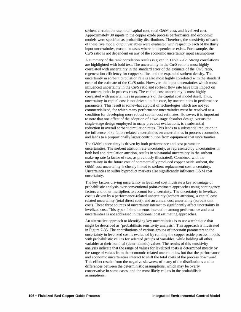
196 •••• Fluidized Bed Copper Oxide Process Integrated Environmental Control Model
sorbent circulation rate, total capital cost, total O&M cost, and levelized cost.Approximately 30 inputs to the copper oxide process performance and economicmodels were specified as probability distributions. Therefore, the sensitivity of eachof these five model output variables were evaluated with respect to each of the thirtyinput uncertainties, except in cases where no dependence exists. For example, theCu/S ratio is not dependent on any of the economic uncertainty input assumptions.
A summary of the rank correlation results is given in Table 7-12. Strong correlationsare highlighted with bold text. The uncertainty in the Cu/S ratio is most highlycorrelated with uncertainty in the standard error of the estimate of the Cu/S ratio,regeneration efficiency for copper sulfite, and the expanded sorbent density. Theuncertainty in sorbent circulation rate is also most highly correlated with the standarderror of the estimate of the Cu/S ratio. However, the input uncertainties which mostinfluenced uncertainty in the Cu/S ratio and sorbent flow rate have little impact onthe uncertainties in process costs. The capital cost uncertainty is most highlycorrelated with uncertainties in parameters of the capital cost model itself. Thus,uncertainty in capital cost is not driven, in this case, by uncertainties in performanceparameters. This result is somewhat atypical of technologies which are not yetcommercialized, for which many performance uncertainties must be resolved as acondition for developing more robust capital cost estimates. However, it is importantto note that one effect of the adoption of a two-stage absorber design, versus thesingle-stage design employed in many previous evaluations, is a substantialreduction in overall sorbent circulation rates. This leads to a substantial reduction inthe influence of sulfation-related uncertainties on uncertainties in process economics,and leads to a proportionally larger contribution from equipment cost uncertainties.
The O&M uncertainty is driven by both performance and cost parameteruncertainties. The sorbent attrition rate uncertainty, as represented by uncertainties inboth bed and circulation attrition, results in substantial uncertainty in the sorbentmake-up rate (a factor of two, as previously illustrated). Combined with theuncertainty in the future cost of commercially produced copper oxide sorbent, theO&M cost uncertainty is closely linked to sorbent replacement cost uncertainty.Uncertainties in sulfur byproduct markets also significantly influence O&M costuncertainty.
The key factors driving uncertainty in levelized cost illustrate a key advantage ofprobabilistic analysis over conventional point-estimate approaches using contingencyfactors and other multipliers to account for uncertainty. The uncertainty in levelizedcost is driven by a performance-related uncertainty (sorbent attrition), a capital costrelated uncertainty (total direct cost), and an annual cost uncertainty (sorbent unitcost). These three sources of uncertainty interact to significantly affect uncertainty inlevelized cost. This type of simultaneous interaction among performance and costuncertainties is not addressed in traditional cost estimating approaches.
An alternative approach to identifying key uncertainties is to use a technique thatmight be described as "probabilistic sensitivity analysis". This approach is illustratedin Figure 7-35. The contributions of various groups of uncertain parameters to theuncertainty in levelized cost is evaluated by running the copper oxide process modelswith probabilistic values for selected groups of variables, while holding all othervariables at their nominal (deterministic) values. The results of this sensitivityanalysis indicate that the range of values for levelized costs is determined mostly bythe range of values from the economic-related uncertainties, but that the performanceand economic uncertainties interact to shift the total costs of the process downward.This effect results from the negative skewness of many of the distributions and todifferences between the deterministic assumptions, which may be overlyconservative in some cases, and the most likely values in the probabilisticassumptions.
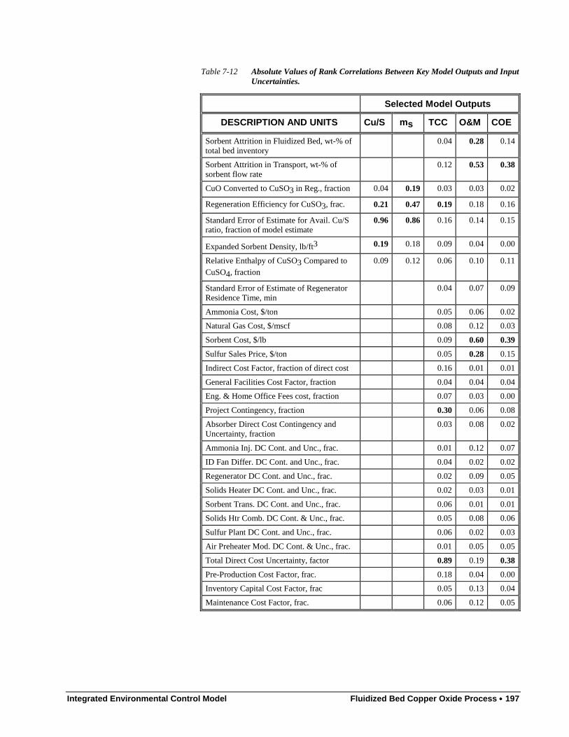
Integrated Environmental Control Model Fluidized Bed Copper Oxide Process •••• 197
Table 7-12 Absolute Values of Rank Correlations Between Key Model Outputs and InputUncertainties.
Selected Model Outputs
DESCRIPTION AND UNITS Cu/S ms TCC O&M COE
Sorbent Attrition in Fluidized Bed, wt-% oftotal bed inventory
0.04 0.28 0.14
Sorbent Attrition in Transport, wt-% ofsorbent flow rate
0.12 0.53 0.38
CuO Converted to CuSO3 in Reg., fraction 0.04 0.19 0.03 0.03 0.02
Regeneration Efficiency for CuSO3, frac. 0.21 0.47 0.19 0.18 0.16
Standard Error of Estimate for Avail. Cu/Sratio, fraction of model estimate
0.96 0.86 0.16 0.14 0.15
Expanded Sorbent Density, lb/ft3 0.19 0.18 0.09 0.04 0.00
Relative Enthalpy of CuSO3 Compared toCuSO4, fraction
0.09 0.12 0.06 0.10 0.11
Standard Error of Estimate of RegeneratorResidence Time, min
0.04 0.07 0.09
Ammonia Cost, $/ton 0.05 0.06 0.02
Natural Gas Cost, $/mscf 0.08 0.12 0.03
Sorbent Cost, $/lb 0.09 0.60 0.39
Sulfur Sales Price, $/ton 0.05 0.28 0.15
Indirect Cost Factor, fraction of direct cost 0.16 0.01 0.01
General Facilities Cost Factor, fraction 0.04 0.04 0.04
Eng. & Home Office Fees cost, fraction 0.07 0.03 0.00
Project Contingency, fraction 0.30 0.06 0.08
Absorber Direct Cost Contingency andUncertainty, fraction
0.03 0.08 0.02
Ammonia Inj. DC Cont. and Unc., frac. 0.01 0.12 0.07
ID Fan Differ. DC Cont. and Unc., frac. 0.04 0.02 0.02
Regenerator DC Cont. and Unc., frac. 0.02 0.09 0.05
Solids Heater DC Cont. and Unc., frac. 0.02 0.03 0.01
Sorbent Trans. DC Cont. and Unc., frac. 0.06 0.01 0.01
Solids Htr Comb. DC Cont. & Unc., frac. 0.05 0.08 0.06
Sulfur Plant DC Cont. and Unc., frac. 0.06 0.02 0.03
Air Preheater Mod. DC Cont. & Unc., frac. 0.01 0.05 0.05
Total Direct Cost Uncertainty, factor 0.89 0.19 0.38
Pre-Production Cost Factor, frac. 0.18 0.04 0.00
Inventory Capital Cost Factor, frac 0.05 0.13 0.04
Maintenance Cost Factor, frac. 0.06 0.12 0.05

198 •••• Fluidized Bed Copper Oxide Process Integrated Environmental Control Model
6 8 10 12 14 16
Levelized Cost (1993 mills/kWh)
0.00
0.25
0.50
0.75
1.00
Cum
ulat
ive
Pro
babi
lity
Performance Only
O&M Cost Only
Capital Cost Only
All Economic
All Uncertainties
Figure 7-35 Uncertainty Result for the Copper Oxide Process Total Levelized Cost.
7.6.4. Evaluating Design Trade-OffsProbabilistically
The significant levels of uncertainty identified in key measures of processperformance suggest that comparisons of design alternatives should be evaluatedtaking into account uncertainties. For example, a key result from the deterministicsensitivity analyses in the previous chapter was that the cost of a two-stage absorber-based system would offer substantial cost savings compared to a single-stageabsorber based system. A nominal cost savings of 1.4 mills/kWh was estimated. Thisresult is revisited using probabilistic assumptions.
The results of a comparison based on the difference in levelized cost for a one-stageabsorber system versus a two-stage absorber system is shown in Figure 7-36. Thedifference is carefully calculated by pairing samples values from two probabilisticsimulations, one for each design option. Because the input uncertainties arecorrelated between the two systems, this pairing is required. The sample values fromthe two-stage simulation were subtracted from the corresponding paired samplevalues for the one-stage system.
The results show considerable uncertainty in the total savings, ranging by a factor ofapproximately four from 0.7 to 2.8 mills/kWh. However, these results do illustratethat there is certain to be a cost savings, and that the cost savings may besubstantially higher than the deterministic estimate.
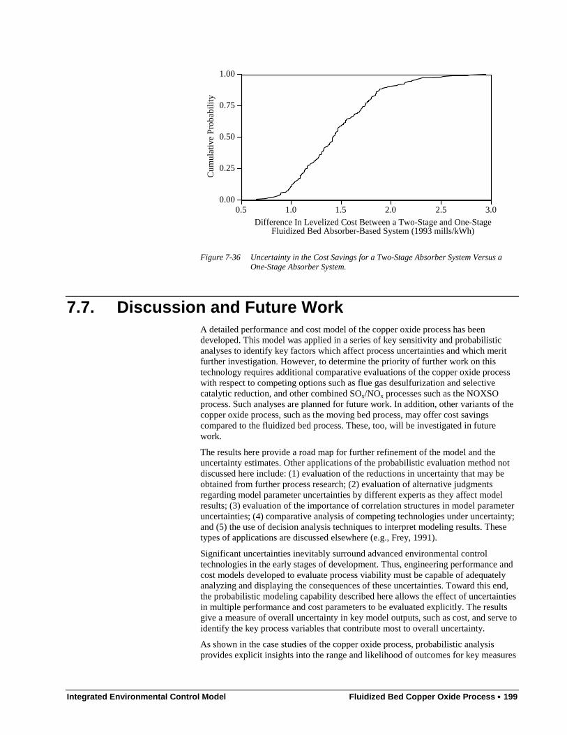
Integrated Environmental Control Model Fluidized Bed Copper Oxide Process •••• 199
0.00
0.25
0.50
0.75
1.00
Cu
mu
lativ
e P
rob
ab
ility
0.5 1.0 1.5 2.0 2.5 3.0
Difference In Levelized Cost Between a Two-Stage and One-Stage Fluidized Bed Absorber-Based System (1993 mills/kWh)
Figure 7-36 Uncertainty in the Cost Savings for a Two-Stage Absorber System Versus aOne-Stage Absorber System.
7.7. Discussion and Future WorkA detailed performance and cost model of the copper oxide process has beendeveloped. This model was applied in a series of key sensitivity and probabilisticanalyses to identify key factors which affect process uncertainties and which meritfurther investigation. However, to determine the priority of further work on thistechnology requires additional comparative evaluations of the copper oxide processwith respect to competing options such as flue gas desulfurization and selectivecatalytic reduction, and other combined SOx/NOx processes such as the NOXSOprocess. Such analyses are planned for future work. In addition, other variants of thecopper oxide process, such as the moving bed process, may offer cost savingscompared to the fluidized bed process. These, too, will be investigated in futurework.
The results here provide a road map for further refinement of the model and theuncertainty estimates. Other applications of the probabilistic evaluation method notdiscussed here include: (1) evaluation of the reductions in uncertainty that may beobtained from further process research; (2) evaluation of alternative judgmentsregarding model parameter uncertainties by different experts as they affect modelresults; (3) evaluation of the importance of correlation structures in model parameteruncertainties; (4) comparative analysis of competing technologies under uncertainty;and (5) the use of decision analysis techniques to interpret modeling results. Thesetypes of applications are discussed elsewhere (e.g., Frey, 1991).
Significant uncertainties inevitably surround advanced environmental controltechnologies in the early stages of development. Thus, engineering performance andcost models developed to evaluate process viability must be capable of adequatelyanalyzing and displaying the consequences of these uncertainties. Toward this end,the probabilistic modeling capability described here allows the effect of uncertaintiesin multiple performance and cost parameters to be evaluated explicitly. The resultsgive a measure of overall uncertainty in key model outputs, such as cost, and serve toidentify the key process variables that contribute most to overall uncertainty.
As shown in the case studies of the copper oxide process, probabilistic analysisprovides explicit insights into the range and likelihood of outcomes for key measures

200 •••• Fluidized Bed Copper Oxide Process Integrated Environmental Control Model
of plant performance and cost. In many cases, there is a probability of obtainingextreme outcomes, such as low performance or high cost, that would result intechnology failure. The characterization of uncertainties in performance and costresults from the simultaneous interaction of uncertainties in many input parameters.These types of insights cannot be obtained from deterministic analysis.
Case studies for the fluidized bed copper oxide process illustrated potentialapplications of an integrated environmental control system framework for processdesign and comparative analyses. Interactions among various components of theenvironmental control system, which are frequently overlooked in many processstudies, were found to significantly influence overall system costs. This is true, forexample, in the case of air preheater modifications to capture the energy released tothe flue gas in the absorber for use in heating the boiler combustion air. Probabilisticcomparisons between advanced and conventional technologies can also providequantitative assessments of the potential benefits and risks of new technology invarious market situations. The potential payoff from process research anddevelopment also may be evaluated using the methods described here.
Of course, as with any other modeling approach, probabilistic methods rely on dataand judgments that must be provided by the user. To be sure, different judgments orassumptions can alter the results. But forcing process developers and evaluators toconsider uncertainties explicitly (rather than ignore them) in probabilisticengineering models can help improve research planning and management byallowing the implications of alternative judgments to be tested. Indeed, experience todate suggests that the process of thinking about key parameter uncertainties, asinputs to a model, often is the most valuable component of this approach that fostersimproved understanding of the systems being modeled.
7.8. NomenclatureA = Fluidized bed area, ft2
Fs = Sorbent feed rate at absorber inlet, fresh sorbent basis, lb/min
GFG = Volumetric flue gas flow rate at absorber inlet, ft3/min
Ib = Bed inventory, lb
ks = Reaction rate constant, 1/(min•atm)
ms = Sorbent mass flow rate, lb/hr
Mi = Molar flow rate of species i, lbmole/hr
Mi,j,k = Molar flow rate of species i at process area j's inlet or outlet k(e.g., MSO2,a,i = molar flow of SO2 at the absorber inlet),lbmole/hr
MWCu = Molecular weight of copper, 63.54 lb/lbmole
MWCuO = Molecular weight of copper oxide, 79.54 lb/lbmole
MWCuSO3 = Molecular weight of copper sulfite, 143.54 lb/lbmole
MWCuSO4 = Molecular weight of copper sulfate, 159.54 lb/lbmole
P = Absorber inlet pressure, atm
rabs = Internal radius of absorber, feet
rves = Radius of steel absorber vessel, feet
Integrated Environmental Control Model Fluidized Bed Copper Oxide Process •••• 201
R = Absorber Inlet Available Cu to inlet SO2 molar ratio, lbmoleCuO/lbmole SO2
thr = Thickness of hot refractory, feet
tir = Thickness of inner or base refractory, feet
tr,a = Absorber solids residence time, min
T = Absorber bed temperature, K
Vs = Superficial flue gas velocity at absorber inlet, ft/sec
WCu = Weight fraction Cu as CuO in fresh sorbent, lb Cu/lb sorbent
x = molar fraction of copper as copper sulfate at the regeneratorinlet
x1 = molar fraction of copper oxide converted to copper sulfite justinside regenerator
yi = SO2 inlet flue gas concentration, lbmoles SO2/lbmole flue gas
yo = SO2 outlet flue gas concentration, lbmoles SO2/lbmole flue gas
Z = Fluidized bed height, ft
7.8.1. Greek Letter Symbolsα = Kinetic parameter (dimensionless)
ηr = Overall sorbent regeneration efficiency, fraction
ηr1 = Regeneration efficiency for copper sulfite, fraction
ηr2 = Regeneration efficiency for copper sulfate, fraction
ηr3 = Regeneration efficiency for copper oxide, fraction
ηs = SO2 removal efficiency, fraction
ρs = Sorbent density (expanded bed), lb/ft3
7.8.2. SubscriptsA = Absorber
Cu = Copper
CuO = Copper Oxide
CuSO3 = Copper Sulfite
CuSO4 = Copper Sulfate
fresh = Sorbent on a fresh basis
i = Inlet
o = Outlet
R = Regenerator
s = Sorbent
SO2 = Sulfur dioxide
202 •••• Fluidized Bed Copper Oxide Process Integrated Environmental Control Model
SO3 = Sulfur trioxide
SOx = All sulfur oxide species
7.9. ReferencesA. E. Roberts and Associates, Inc. (1994). Conceptual Design and EconomicEvaluation of the Fluidized Bed Copper Oxide Process. Prepared for UOP, Inc. andthe U.S. Department of Energy. March.
Barin, I., and O. Knacke (1973). Thermochemical Properties of InorganicSubstances. Springer-Verlag, New York.
Barin, I., O. Knacke, and O. Kubaschewski (1977). Thermochemical Properties ofInorganic Substances: Supplement. Springer-Verlag, New York.
Chase., M.W., et al. (1985). "JANAF Thermochemical Tables, Third Edition, Part11, Cr-Zr," Journal of Physical and Chemical Reference Data, Vol. 14, SupplementNo. 1.
Demski, R. J., S.J. Gasior, E. R. Bauer, Jr., J. T. Yeh, J.P. Strakey, and J.I. Joubert(1982). "Simultaneous Removal of SO2 and NOx From Flue Gas Employing aFluidized-Bed Copper Oxide Process," 1982 Summer Session of AIChE, August 29to September 1.
Drummond, C. J., J. T. Yeh, J.I. Joubert, and J. A. Ratafia-Brown (1985). TheDesign of a Dry, Regenerative Fluidized Bed Copper Oxide Process for the Removalof Sulfur Dioxide and Nitrogen Oxides from Coal-Fired Boilers. Presented at the78th Annual Meeting of the Air Pollution Control Association, June 16-21.
Frey, H. C. (1987). Performance and Economic Model of the Fluidized Bed CopperOxide Process. Master's Thesis. Department of Mechanical Engineering, Carnegie-Mellon University. Pittsburgh, PA. May.
Frey, H. C., E.S. Rubin, and J.S. Salmento (1989), "Evaluation of the Fluidized BedCopper Oxide Process Using A Probabilistic Engineering Model," Proceedings ofthe Sixth Annual International Pittsburgh Coal Conference, Pittsburgh,Pennsylvania, p. 356-365.
Frey, H. C., and E.S. Rubin (1991), "Probabilistic Evaluation of Advanced SO2/NOxControl Technology," Journal of the Air and Waste Management Association,41(12):1585-1593 (December).
Frey, H. C., and E.S. Rubin (1992), "An Evaluation Method for Advanced Acid RainCompliance Technology," Journal of Energy Engineering, 118(1):38-55 (April).
Frey, H. C., and E.S. Rubin (1992a), "Evaluation of Advanced Coal GasificationCombined-Cycle Systems Under Uncertainty," Industrial and EngineeringChemistry Research, 31(5):1299-1307.
Frey, H. C., E.S. Rubin, and U.M. Diwekar (1994), "Modeling Uncertainties inAdvanced Technologies: Application to a Coal Gasification System with Hot GasCleanup," Energy 19(4):449-463.
Harriott, P. (1992a). Personal Communication to D. Henzel, June 3.
Harriott, P. (1992b). Personal Communication to D. Henzel, August 4.
Harriott, P. (1992c). Personal Communication to C. Frey, August 14.
Integrated Environmental Control Model Fluidized Bed Copper Oxide Process •••• 203
Harriott, P., and J.M. Markussen (1992), "Kinetics of Sorbent Regeneration in theCopper Oxide Process for Flue Gas Cleanup," Industrial and Engineering ChemistryResearch, 31(1):373-379.
Merrow, E.W., K.E. Phillips, and C.W. Myers (1981). Understanding Cost Growthand Performance Shortfalls in Pioneer Process Plants. Prepared by Rand Corporationfor U.S. Department of Energy.
Plantz, A. R., C. J. Drummond, S. W. Hedges, and F.N. Gromicko (1986).Performance of the Fluidized Bed Copper Oxide Process in an Integrated TestFacility. Presented at the 79th Annual Meeting of the Air Pollution ControlAssociation, Minneapolis, Minnesota. June 22-27.
Rubin, E.S., J.S. Salmento, J.G. Barrett, C.N. Bloyd, and H. C. Frey (1986).Modeling and Assessment of Advanced Processes for Integrated EnvironmentalControl of Coal-Fired Power Plants. Prepared by the Center for Energy andEnvironmental Studies, Carnegie-Mellon University, for the U.S. Department ofEnergy. July.
Rubin, E.S., J.S. Salmento, and H. C. Frey (1988). Cost-Effective Emission Controlsfor Coal-Fired Power Plants. Chemical Engineering Communications, 74. pp. 155-167. December
Rubin, E.S., J.S. Salmento, and H. C. Frey (1989), "Evaluating Combined SO2/NO2
Processes," Proceedings: Fourth Symposium on Integrated Environmental Control,Electric Power Research Institute, Palo Alto, California, EPRI Report No. GS-6519,September, p. 6-1 to 6-15.
Rubin, E.S., J.S. Salmento, H. C. Frey, A. Abu-Baker, and M. Berkenpas (1991),Modeling of Integrated Environmental Control Systems for Coal-Fired PowerPlants, Final Report (draft), submitted by Carnegie-Mellon University to the U.S.Department of Energy, Pittsburgh, Pennsylvania, DOE Contract No. DE-AC22-87PC79864, April, 214p.
Rubin, E.S., H. C. Frey, and M. B. Berkenpas (1992), "Development of theIntegrated Environmental Control Model," Proceedings, Eighth Annual CoalPreparation, Utilization, and Environmental Control Contractor's Conference, U.S.Department of Energy, Pittsburgh, Pennsylvania, July 27-30, pp. 619-626.
SMC (1983a). Technical and Economic Evaluation of the Fluidized Bed CopperOxide Flue Gas Treatment Process and Integrated Sulfur-Producing Plants. Preparedby Science Management Corporation for the U.S. Department of Energy, PittsburghEnergy Technology Center, Pittsburgh, PA. June.
SMC (1983b). Technical and Economic Evaluation of Design Optimization IssuesAssociated With the Fluidized Bed Copper Oxide Flue Gas Treatment Process.Prepared by Science Management Corporation for the U.S. Department of Energy,Pittsburgh, PA. November.
SMC (1983c). Economic Evaluation of the Fluidized Bed Copper Oxide Flue GasTreatment Process and Integrated Sulfuric Acid Plant. Prepared by ScienceManagement Corporation for the U.S. Department of Energy, Pittsburgh, PA. April.
SMC (1984). Modeling of the Regenerator Reactor for the Fluidized Bed CopperOxide Flue Gas Treatment Process. Prepared by Science Management Corporationfor the U.S. Department of Energy, Pittsburgh, PA. May.
Williamson, R.R., J. A. Morici, and T.L LaCosse (1987). Sorbent Life CycleTesting, Fluidized Bed Copper Oxide Process. Prepared by UOP, Inc., for the U.S.Department of Energy, Pittsburgh, PA.

204 •••• Fluidized Bed Copper Oxide Process Integrated Environmental Control Model
Yeh, J. T., C. J. Drummond, and J.I. Joubert (1987), "Process Simulation of theFluidized-Bed Copper Oxide Process Sulfation Reaction," Environmental Progress,6(2):44-50.
Yeh, J. T., R. J. Demski, J.P. Strakey, and J.I. Joubert (1984). "PETC Fluidized-BedCopper Oxide Process for Combined SO2/NOx Removal from Flue Gas," AIChE1984 Winter National Meeting, Atlanta, March 11-14.
7.10. Appendix A. Technical Background on the CuOProcess
This section provides a brief overview of the fluidized bed copper oxide process tofamiliarize you with the system we are modeling and to help ensure that we all havea common framework for discussing uncertainties in the process. More detail aboutthe process and the models we employ can be found in the following papers andreports, which you may already have:
6. Frey, H. C., "Performance Model of the Fluidized Bed Copper OxideProcess for SO2/NOx Control," Paper 93-WA-79.01 presented at the86th Annual Meeting of the Air & Waste Management Association,Denver, CO, June 13-18, 1993.
7. Frey, H. C., and E.S. Rubin, "An Evaluation Method for AdvancedAcid Rain Compliance Technology," Journal of Energy Engineering,118(1):38-55 (April 1992).
8. Frey, H. C., and E.S. Rubin, "Probabilistic Evaluation of AdvancedSO2/NOx Control Technology," Journal of the Air and WasteManagement Association, 41(12):1585-1593 (December 1991).
9. Rubin, E.S., M. B. Berkenpas, and H. C. Frey, "Development of theIntegrated Environmental Control Model," Proceedings, Ninth AnnualCoal Preparation, Utilization, and Environmental Control Contractor'sConference, U.S. Department of Energy, Pittsburgh, Pennsylvania, July19-22, 1993, pp. 447-454.
10. Rubin, E.S., J.S. Salmento, H. C. Frey, A. Abu-Baker, and M.Berkenpas, Modeling of Integrated Environmental Control Systems forCoal-Fired Power Plants, Final Report, Prepared by Carnegie-MellonUniversity for the U.S. Department of Energy, Pittsburgh,Pennsylvania, DOE Contract No. DE-AC22-87PC79864, April 1991,214p.
11. Rubin, E.S., J.S. Salmento, J.G. Barrett, C.N. Bloyd, and H. C. Frey,Modeling and Assessment of Advanced Processes for IntegratedEnvironmental Control of Coal-Fired Power Plants, prepared byCarnegie-Mellon University for the U.S. Department of Energy,Pittsburgh, Pennsylvania, NTIS DE86014713, July 1986.
Of these, the first paper cited here is the most relevant. It contains documentation ofthe newest version of the copper oxide performance model, and several illustrativedeterministic case studies. It is assumed here that you are already thoroughly familiarwith the fluidized bed copper oxide. Furthermore, it is also assumed that you haveaccess to the first paper referenced above and can review it to familiarize yourselfwith the performance model.
A process schematic is included on the following page. Some key designassumptions are given in the next section.
Integrated Environmental Control Model Fluidized Bed Copper Oxide Process •••• 205
7.11. Appendix B. Questions About PerformanceUncertainties in the Copper Oxide Process
Here, you are asked to provide technically-informed judgments about probabilitydistributions for parameters of a performance model for the fluidized bed copperoxide process. You are asked to consider the possibilities of potentially poorperformance as well as the probability of obtaining favorable performance, based oncurrent information about the system. The preceding sections provide an overview ofuncertainty analysis and sources of technical information about the process and themodels we employ.
We are interested in your technically-based judgments about uncertainties in keyperformance parameters related primarily to absorption, regeneration, sorbenttransport and attrition, and process design. We intend to model the uncertainty inperformance and cost associated with a fifth-of-a-kind, or mature, system. Thus, weare asking you to make predictions about systems that have not yet been built oroperated. We are asking you to express the range of possible outcomes for thesesystems using probability distributions, as discussed in Part 1.
Several questions follow. These are the types of questions which we will discuss onFriday. If you would like, you may respond to the questions on these pages, or useadditional paper as needed. Alternatively, you could provide your responses moreinformally during our meeting on Friday. See the Introduction for examples of howyou might estimate uncertainty in each parameter.
7.11.1. Design AssumptionsA number of key design assumptions for the fluidized bed copper oxide process areshown in Table 7-13.
In previous work reported by Frey at the last AWMA meeting, three integrationstrategies are considered for the copper oxide process and a sulfuric acid plant. Case1 represents a base case in which no measures are taken to correct for Claus planttailgas emissions. In Case 2, the SO2 removal efficiency in the absorber is increasedto compensate for the tailgas emissions. In Case 3, the tailgas emissions are recycledto the flue gas just upstream of the absorber, and the absorber sulfur removalefficiency is increased slightly to achieve an overall 90 percent removal efficiency.Cases 2 and 3 yield the same overall removal efficiency of 90 percent, while Case 1achieves only 85.5 percent removal efficiency. The design assumptions for SO2
removal efficiencies in Table 7-13 are based on Case 3.

206 •••• Fluidized Bed Copper Oxide Process Integrated Environmental Control Model
Table 7-13 Key Copper Oxide Process Design Assumptions
Parameter Value
Absorber Process Area
Required SO2 Removal Efficiency, % 90.0
Absorber SO2 Removal Efficiency, % 90.5
Sulfur Plant Recovery Efficiency, % 95.0
Claus Tailgas Recycle to Flue Gas Yes
Overall SO2 Removal Efficiency, % 90.0
NOx Removal Efficiency, % 90.0
Flue Gas Inlet Temp., oF 705
Number of Absorbers 2
NH3/NOx Molar Ratio 1.00
Superficial Flue Gas Velocity (ft/s) 4.5
Expanded Bed Height (inches) 48
Expanded Sorbent Density, lb/ft3 26.6
Fluidized Bed Pressure Drop (in. H2O) 27.7
Regenerator Process Area
CuO Regeneration Efficiency, % 80
CuSO4 Regeneration Efficiency, % 80
CuSO3 Regeneration Efficiency, % 80
Conversion of CuO to CuSO3, frac. 1
Regenerator Inlet Temperature, °F 900
Regenerator Methane/CuSO4 Ratio 1.15
Methane Inlet Temperature, °F. 77
System Parameters
Sorbent Copper Loading (wt-%) 7
Bed Attrition (%/hr of bed inventory) 0.020
Circulation Attrition (% of circulation) 0.047
Key Coal Properties
Sulfur Content, wt-% 3.12
7.11.1.1. Question #1: Comments on Default AssumptionsDo the default assumptions seem reasonable? If not, adjust accordingly and explainthe basis for the changes. Are there additional assumptions that should be specifiedfor these systems? If so, please add these assumptions and explain why they areneeded. Use your updated set of assumptions as the basis for answering thefollowing questions.
7.11.1.2. Question #2. Uncertain Parameter IdentificationThe following is a list of the specific parameters for which uncertainty distributionsare desired.
Absorber-Related Uncertainties
• Sulfation Rate Constant Model Error
Integrated Environmental Control Model Fluidized Bed Copper Oxide Process •••• 207
• Cu/S Model Error
• Fluidized Bed Sorbent Density
• Fluidized Bed Flue Gas Pressure Drop
• Dependency on fluidized bed height (over a range of 36 to 72 inches)
• Ammonia Stoichiometry and Ammonia Slip
Regeneration-Related Uncertainties
• Formation of CuSO3 in the regenerator
• Regeneration Efficiencies for Different Copper Species
12. • Copper Oxide
13. • Copper Sulfite
14. • Copper Sulfate
• Regenerator Residence Time Model Error
• Regenerator Rate Constant for CuSO4
• Regenerator Reaction Rate for CuSO4
Other Uncertainties
• Sorbent Attrition Rate
15. • dependency on sorbent copper loading (over a range of 5to 10 wt-% Cu as CuO)
16. • dependency on fluidized bed height (over a range of 36 to72 inches)
• Sorbent Unit Cost
Are you comfortable making estimates of uncertainty for these parameters?
Are there other parameters which you believe also should be treated probabilistically(whether or not you feel comfortable making the judgment yourself) that are notincluded in the above list? If so, please specify what these parameters are and supplyyour judgments about them if you are comfortable doing so (see the followingquestions for examples of the types of judgments we are looking for). If not, who canwe ask to estimate uncertainties for these additional parameters?
Absorber-Related Uncertainties
Uncertainty in Sulfation Rate Constant Model
The expression used in the model to calculate the rate constant is:
ks =1,573 exp(-14.23 WCu)exp −2,417.6
T
where ks is the reaction rate constant (1/(min*atm)), WCu is the sorbent copperloading (wt-fraction Cu as CuO), and T is the absorber bed temperature (K). Clearly,this model provides an estimate of the actual rate constant under different conditionsof sorbent copper loading and temperature. How accurate and precise is the model?Accuracy refers to random error in predicting the rate constant, whereas precisionrefers to any biases (e.g., a systematic tendency to under-predict or over-predict).How likely is it that the rate constant could be higher than the estimated value? How
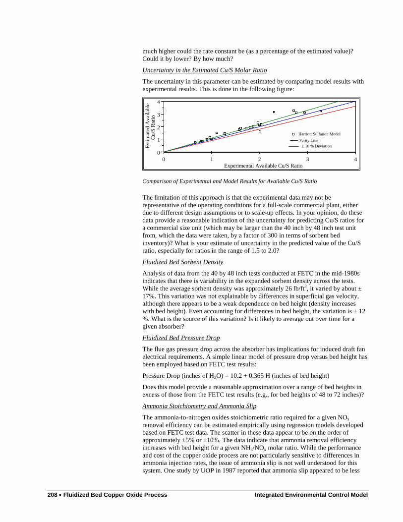
208 •••• Fluidized Bed Copper Oxide Process Integrated Environmental Control Model
much higher could the rate constant be (as a percentage of the estimated value)?Could it by lower? By how much?
Uncertainty in the Estimated Cu/S Molar Ratio
The uncertainty in this parameter can be estimated by comparing model results withexperimental results. This is done in the following figure:
432100
1
2
3
4
Harriott Sulfation Model
Parity Line
Experimental Available Cu/S Ratio
Est
imat
ed A
vaila
ble
C
u/S
Ra
tio± 10 % Deviation
Comparison of Experimental and Model Results for Available Cu/S Ratio
The limitation of this approach is that the experimental data may not berepresentative of the operating conditions for a full-scale commercial plant, eitherdue to different design assumptions or to scale-up effects. In your opinion, do thesedata provide a reasonable indication of the uncertainty for predicting Cu/S ratios fora commercial size unit (which may be larger than the 40 inch by 48 inch test unitfrom, which the data were taken, by a factor of 300 in terms of sorbent bedinventory)? What is your estimate of uncertainty in the predicted value of the Cu/Sratio, especially for ratios in the range of 1.5 to 2.0?
Fluidized Bed Sorbent Density
Analysis of data from the 40 by 48 inch tests conducted at FETC in the mid-1980sindicates that there is variability in the expanded sorbent density across the tests.While the average sorbent density was approximately 26 lb/ft3, it varied by about ±17%. This variation was not explainable by differences in superficial gas velocity,although there appears to be a weak dependence on bed height (density increaseswith bed height). Even accounting for differences in bed height, the variation is ± 12%. What is the source of this variation? Is it likely to average out over time for agiven absorber?
Fluidized Bed Pressure Drop
The flue gas pressure drop across the absorber has implications for induced draft fanelectrical requirements. A simple linear model of pressure drop versus bed height hasbeen employed based on FETC test results:
Pressure Drop (inches of H2O) = 10.2 + 0.365 H (inches of bed height)
Does this model provide a reasonable approximation over a range of bed heights inexcess of those from the FETC test results (e.g., for bed heights of 48 to 72 inches)?
Ammonia Stoichiometry and Ammonia Slip
The ammonia-to-nitrogen oxides stoichiometric ratio required for a given NOx
removal efficiency can be estimated empirically using regression models developedbased on FETC test data. The scatter in these data appear to be on the order ofapproximately ±5% or ±10%. The data indicate that ammonia removal efficiencyincreases with bed height for a given NH3/NOx molar ratio. While the performanceand cost of the copper oxide process are not particularly sensitive to differences inammonia injection rates, the issue of ammonia slip is not well understood for thissystem. One study by UOP in 1987 reported that ammonia slip appeared to be less
Integrated Environmental Control Model Fluidized Bed Copper Oxide Process •••• 209
than 50 ppmv. However, such levels could be excessive. For 90 percent NOx
removal, what is your best estimate as to best case, worst case, and most likelyammonia slip levels?
Regenerator-Related Uncertainties
Formation of CuSO3 in the Regenerator
Some studies have suggested that potentially many other copper species besides Cu,CuO, and CuSO4 may play an important role, particularly with regard toregeneration. For example, CuSO3 may be formed by the reaction of SO2 in theexiting off-gas with CuO in the incoming sorbent. The question here is: how much(if any) CuSO3 is formed in this manner?
Regeneration Efficiencies
A key input to the regenerator kinetic model used to estimate required sorbentresidence time is the regeneration efficiency of CuSO4. This parameter is assumed tohave a value of 80 percent in the default design basis.
What is the relationship between the regeneration efficiency of CuSO3 and that ofCuSO4? For example, Harriott and Markussen (IECR, 31:1, p.378) indicate that theregeneration efficiency of CuSO3 could be substantially less than that of CuSO4.
What is the relationship between the regeneration of CuO and CuSO4? What arereasonable assumptions to make? What ranges of values can be used? For example,is the regeneration efficiency for CuO the same as for CuSO4?
Regenerator Residence Time Model
How accurate and precise are predictions made by the regenerator residence timemodel described in Frey's paper (the model itself was developed by Harriott based onexperimental work done by Harriott and Markussen). Assuming that all inputs to themodel were known with certainty, how much scatter could we expect to see betweenmodel predictions and actual process performance? What are some sources ofdiscrepancies (e.g., channeling of flow with the regenerator bed, masking bycontaminants, unaccounted for chemical reactions, etc.)? How much longer could theresidence time be, as a percentage of the model estimate? How much lower?
Regenerator Rate Constant
How accurate and precise are the predictions of the rate constant for the regenerationof copper sulfate? These predictions are given by the following model:
°
−×××
°≤
−×××
=
R1,355>T if 800,16
exp1011.2
R1,355T if 700,21
exp102.4
5
7
,
TF
TF
k
w
w
rs
where the factor Fw is a correction based on the sorbent copper loading:
) W23.14exp(04.2 Cu−=wF
For example, as a percentage of the value estimated by the model, how much highermight the actual rate constant be? How much lower might it be?
Regenerator Reaction Rate
The copper sulfate regeneration reaction rate is estimated using the followingexpression, based on a memo by Harriott. The reaction rate is estimated for each of a
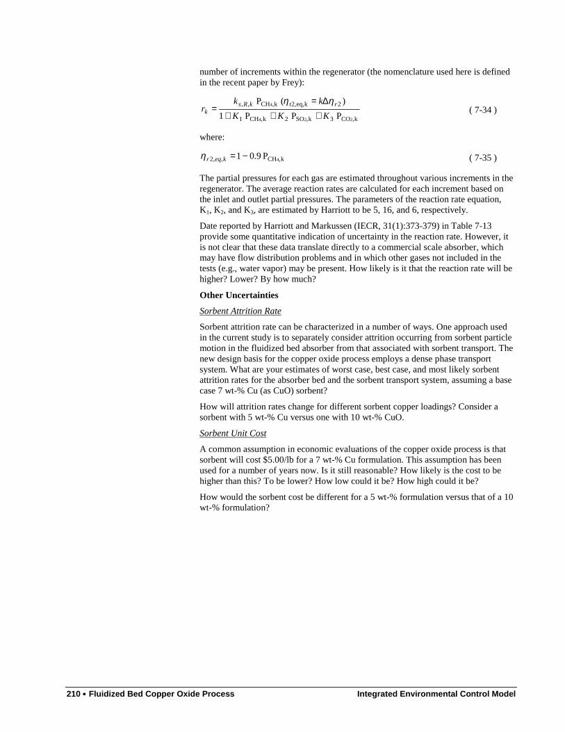
210 •••• Fluidized Bed Copper Oxide Process Integrated Environmental Control Model
number of increments within the regenerator (the nomenclature used here is definedin the recent paper by Frey):
k,CO3k,SO2k,CH1
2keq,r2,k,CH,,
224
4
P P P 1
)( P
KKK
kkr
rkRsk +++
∆==
ηη( 7-34 )
where:
k,CH,,2 4P 9.01−=keqrη ( 7-35 )
The partial pressures for each gas are estimated throughout various increments in theregenerator. The average reaction rates are calculated for each increment based onthe inlet and outlet partial pressures. The parameters of the reaction rate equation,K1, K2, and K3, are estimated by Harriott to be 5, 16, and 6, respectively.
Date reported by Harriott and Markussen (IECR, 31(1):373-379) in Table 7-13provide some quantitative indication of uncertainty in the reaction rate. However, itis not clear that these data translate directly to a commercial scale absorber, whichmay have flow distribution problems and in which other gases not included in thetests (e.g., water vapor) may be present. How likely is it that the reaction rate will behigher? Lower? By how much?
Other Uncertainties
Sorbent Attrition Rate
Sorbent attrition rate can be characterized in a number of ways. One approach usedin the current study is to separately consider attrition occurring from sorbent particlemotion in the fluidized bed absorber from that associated with sorbent transport. Thenew design basis for the copper oxide process employs a dense phase transportsystem. What are your estimates of worst case, best case, and most likely sorbentattrition rates for the absorber bed and the sorbent transport system, assuming a basecase 7 wt-% Cu (as CuO) sorbent?
How will attrition rates change for different sorbent copper loadings? Consider asorbent with 5 wt-% Cu versus one with 10 wt-% CuO.
Sorbent Unit Cost
A common assumption in economic evaluations of the copper oxide process is thatsorbent will cost $5.00/lb for a 7 wt-% Cu formulation. This assumption has beenused for a number of years now. Is it still reasonable? How likely is the cost to behigher than this? To be lower? How low could it be? How high could it be?
How would the sorbent cost be different for a 5 wt-% formulation versus that of a 10wt-% formulation?

Integrated Environmental Control Model NOXSO Process •••• 211
8. NOXSO Process
8.1. IntroductionThe NOXSO process is an advanced technology that removes both SO2 and NOx
simultaneously using a sorbent prepared by spraying sodium carbonate on thesurface of γ-alumina spheres. It is designed to achieve SO2 removal efficienciesabove 90% and NOx removal at levels above 80%. The main features of this processare:
• Simultaneous SO2 and NOx removal in a single absorber vessel
• Regenerative use of sorbent, thereby avoiding the production of liquidor solid waste
• Production of a saleable byproduct in the form of sulfur or sulfuric acid
The NOXSO process was developed in the early 1980s and successfullydemonstrated at the small-scale (0.17 MW) in 1983-85 at TVA’s Shawnee SteamPlant facility (Haslbeck & Neal, 1985; Yates, 1983). This was followed by ProcessDevelopment Unit (PDU) tests on a slightly larger scale (0.75 MW) in cooperationwith USDOE FETC in the mid-eighties. A Life-Cycle Test Unit (LCTU) was built(0.06 MW) in 1988 to examine the NOXSO process in an integrated continuousmode operation (Yeh, Drummond, Haslbeck, & Neal, 1987; Yeh, Ma, Pennline,Haslbeck, & Gromicko, 1990). Finally a Proof-of-Concept (POC) unit was built inthe early 1990s at a 5 MW scale as the last test before full-scale demonstration(Black, Woods, Friedrich, & Leonard, 1993; Ma, 1994-95; Ma, Haslbeck, et. al.,1993). Based on these tests, conceptual designs of commercial scale units are nowbeing developed.
There are several similarities between the NOXSO process and the fluidized bedcopper oxide process another integrated emission control technology supported byUSDOE FETC and modeled in the IECM. The key differences between theseprocesses are twofold:
1. NOXSO uses a sorbent that consists of sodium carbonate sprayed onthe surface of γ-alumina spheres while the CuO process uses copperoxide as a sorbent. The latter requires operation at high temperaturesupstream of the air preheater, where the NOXSO catalyst operates atlower temperatures downstream of the preheater.
2. NOXSO recycles the NOx removed from the flue gas back to thefurnace along with combustion air. By injecting it into the fuel-richhigh temperature combustion zone it is decomposed to N2 and O2. The
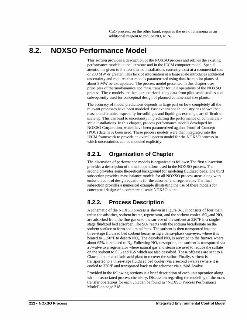
212 •••• NOXSO Process Integrated Environmental Control Model
CuO process, on the other hand, requires the use of ammonia as anadditional reagent to reduce NOx to N2.
8.2. NOXSO Performance ModelThis section provides a description of the NOXSO process and refines the existingperformance models in the literature and in the IECM computer model. Specialattention is given to the fact that no installations currently exist at a commercial sizeof 200 MW or greater. This lack of information at a large scale introduces additionaluncertainty and requires that models parametrized using data from pilot plants ofabout 5 MW be extrapolated. The process model presented in this chapter usesprinciples of thermodynamics and mass transfer for unit operations of the NOXSOprocess. These models are then parametrized using data from pilot scale studies andsubsequently used for conceptual design of planned commercial size plants.
The accuracy of model predictions depends in large part on how completely all therelevant processes have been modeled. Past experience in industry has shown thatmass transfer units, especially for solid-gas and liquid-gas exchange, are difficult toscale up. This can lead to uncertainty in predicting the performance of commercial-scale installations. In this chapter, process performance models developed byNOXSO Corporation, which have been parametrized against Proof-of-Concept(POC) data have been used. These process models were then integrated into theIECM framework to provide an overall system model for the NOXSO process inwhich uncertainties can be modeled explicitly.
8.2.1. Organization of ChapterThe discussion of performance models is organized as follows: The first subsectionprovides a description of the unit operations used in the NOXSO process. Thesecond provides some theoretical background for modeling fluidized beds. The thirdsubsection provides mass balance models for all NOXSO process areas along withemission control design equations for the adsorber and regenerator. The finalsubsection provides a numerical example illustrating the use of these models forconceptual design of a commercial scale NOXSO plant.
8.2.2. Process DescriptionA schematic of the NOXSO process is shown in Figure 8-1. It consists of four mainunits: the adsorber, sorbent heater, regenerator, and the sorbent cooler. SO2 and NOx
are adsorbed from the flue gas onto the surface of the sorbent at 320°F in a single-stage fluidized bed adsorber. The SO2 reacts with the sodium bicarbonate on thesorbent surface to form sodium sulfates. The sorbent is then transported into thethree-stage fluidized bed sorbent heater using a dense-phase conveyer, where it isheated to 1150°F to desorb NOx. The desorbed NOx is recycled to the furnace whereabout 65% is reduced to N2. Following NOx desorption, the sorbent is transported viaa J-valve to a regenerator where natural gas and steam are used to reduce the sulfateon the sorbent to SO2 and H2S which are also desorbed. These offgases are sent to aClaus plant or a sulfuric acid plant to recover the sulfur. Finally, sorbent istransported to a three-stage fluidized bed cooler (via a second J-valve) where it iscooled to 320°F and transported back to the adsorber via a third J-valve.
Provided in the following sections is a brief description of each unit operation alongwith its associated process chemistry. Discussion regarding the modeling of the masstransfer operations for each unit can be found in "NOXSO Process PerformanceModel" on page 218.

Integrated Environmental Control Model NOXSO Process •••• 213
8.2.2.1. AdsorberThe adsorber consists of a single-stage fluidized bed containing the Na2CO3 coveredγ-alumina beads of 1/16 inch diameter. The operating temperature of the bed is320°F at which temperature Na2CO3 is reduced to Na2O. If necessary, the flue gas isfirst cooled to 320°F by spraying water into the flue gas ducts. It then passes throughthe adsorber at a superficial velocity at least as large as the minimum fluidizationvelocity. The SO2 and NOx in the flue gas are adsorbed onto the surface of thealumina beads via solid-gas mass transfer.
���������������������� ���������������������������� ����������������������������������
������������������������������������������
�������������������������������������������������������������
������������������������������������������������
water
������������������������������������������������������������������
�������������������� ��
��������������������������������������
Combustion AirCoal
���������������������
��������
����������������
�����������������������������������������������������������������������������������������
�������������
#6 Fuel Oil (Oil_airheater) Air (Air_airheater)
Air
����������
��������
����
������
�����������������������������������������
������������ ���������������������� ������������������������������������������������������������������������������������������������������������������������������������������������������������������������������������������������������������������������������������������������������������������������������������������������������������������������������������������������������������������������������������������������������������������������������������������������������������������������������������������������������������������������������������������������������������������������������������������������������������������������������������������������������������������������������������������������
Sulfuric Acid (sul_acid)
Steam (msteam_sul, Temo_steam)
Methane (Mch4rin)
Low Pressure Steam (Mh2orin)
Acid Plant
Air Heater
Sorbent Heater
RegeneratorSorbent Cooler
Air Preheater
Adsorber
Sorbent
Flue Gas
Regenerator Off-Gas (Gasregout, Trout, Prout)
Boiler
���
��������
��
Makeup Sorbent (Makeup_sorbent)
Sor
bent
(M
saou
t, T
aout
)
Heater Gas (Gas_to_furnace, 620F)
(Gasnoxsoin, Noxso_temp, Noxsoinsolids)
(Air_sorbent, 610F)
(Gascool, Tain)
(Gasnoxsoout, Taout, Noxsooutsolids)
Tshout, Mso2rin
Figure 8-1 A Schematic of the NOXSO Process Flowsheet
Based on laboratory experiments and the results obtained from the POC tests theproposed mechanism for the SO2/NOx adsorption is as follows:
3222 SONa SO +ONa ⇔ ( 8-1 )
4232 NaSO O 1/2 + SONa ⇔ ( 8-2 )
242222 NO + SONa O + NO + SO + ONa ⇔ ( 8-3 )
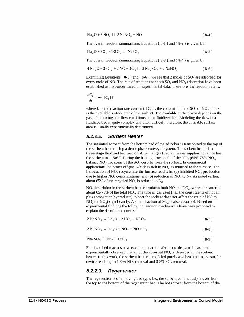
214 •••• NOXSO Process Integrated Environmental Control Model
NO + NaNO 2 NO 3 + ONa 322 ⇔ ( 8-4 )
The overall reaction summarizing Equations ( 8-1 ) and ( 8-2 ) is given by:
4222 NaSO O 1/2+ SO + ONa ⇔ ( 8-5 )
The overall reaction summarizing Equations ( 8-3 ) and ( 8-4 ) is given by:
342222 NaNO 2 + SONa 3 O 3 + NO 2 + SO 3 + ONa 4 ⇔ ( 8-6 )
Examining Equations ( 8-5 ) and ( 8-6 ), we see that 2 moles of SO2 are adsorbed forevery mole of NO. The rate of reactions for both SO2 and NOx adsorption have beenestablished as first-order based on experimental data. Therefore, the reaction rate is:
SCkdt
dCii
i ][−=
where ki is the reaction rate constant, [Ci] is the concentration of SO2 or NOx, and Sis the available surface area of the sorbent. The available surface area depends on thegas-solid mixing and flow conditions in the fluidized bed. Modeling the flow in afluidized bed is quite complex and often difficult, therefore, the available surfacearea is usually experimentally determined.
8.2.2.2. Sorbent HeaterThe saturated sorbent from the bottom bed of the adsorber is transported to the top ofthe sorbent heater using a dense phase conveyor system. The sorbent heater is athree-stage fluidized bed reactor. A natural gas fired air heater supplies hot air to heatthe sorbent to 1150°F. During the heating process all of the NOx (65%-75% NO2,balance NO) and some of the SO2 desorbs from the sorbent. In commercialapplications the heater off-gas, which is rich in NOx, is returned to the furnace. Theintroduction of NOx recycle into the furnace results in: (a) inhibited NOx productiondue to higher NOx concentrations, and (b) reduction of NOx to N2. As noted earlier,about 65% of the recycled NOx is reduced to N2.
NOx desorbtion in the sorbent heater produces both NO and NO2, where the latter isabout 65-75% of the total NOx. The type of gas used (i.e., the constituents of hot airplus combustion byproducts) to heat the sorbent does not affect the ratio of NO toNO2 (in NOx) significantly. A small fraction of SO2 is also desorbed. Based onexperimental findings the following reaction mechanisms have been proposed toexplain the desorbtion process:
2223 O 1/2+ NO 2+ ONa NaNO 2 → ( 8-7 )
2223 O+ NO + NO + ONa NaNO 2 → ( 8-8 )
2232 SO + ONa SONa ⇔ ( 8-9 )
Fluidized bed reactors have excellent heat transfer properties, and it has beenexperimentally observed that all of the adsorbed NOx is desorbed in the sorbentheater. In this work, the sorbent heater is modeled purely as a heat and mass transferdevice resulting in 100% NOx removal and 0-5% SO2 removal.
8.2.2.3. RegeneratorThe regenerator is of a moving bed type, i.e., the sorbent continuously moves fromthe top to the bottom of the regenerator bed. The hot sorbent from the bottom of the
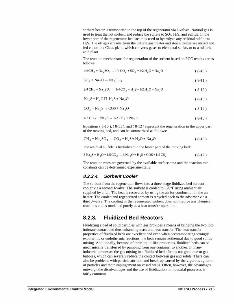
Integrated Environmental Control Model NOXSO Process •••• 215
sorbent heater is transported to the top of the regenerator via J-valves. Natural gas isused to treat the hot sorbent and reduce the sulfate to SO2, H2S, and sulfide. In thelower part of the regenerator bed steam is used to hydrolyze any residual sulfide toH2S. The off-gas streams from the natural gas treater and steam treater are mixed andfed either to a Claus plant, which converts gases to elemental sulfur, or to a sulfuricacid plant.
The reaction mechanisms for regeneration of the sorbent based on POC results are asfollows:
ONa + OH 1/2+ SO + CO 1/4 SONa + CH 1/4 2222424 → ( 8-10 )
3222 SONa ONa + SO → ( 8-11 )
ONa + OH 1/2 + SH + CO 3/4 SONa + CH 3/4 2222324 → ( 8-12 )
ONa + SH OH + SNa 2222 ⇔ ( 8-13 )
ONa + COS SNa + CO 222 → ( 8-14 )
ONa + CS 1/2 SNa + CO 1/2 2222 → ( 8-15 )
Equations ( 8-10 ), ( 8-11 ), and ( 8-12 ) represent the regeneration in the upper partof the moving bed, and can be summarized as follows:
ONa +OH + SH + CO SONa + CH 2222424 → ( 8-16 )
The residual sulfide is hydrolized in the lower part of the moving bed:
222222 CS 1/2+ COS + SH + ONa 3 CO 1.5 + OH + SNa 3 → ( 8-17 )
The reaction rates are governed by the available surface area and the reaction rateconstants can be determined experimentally.
8.2.2.4. Sorbent CoolerThe sorbent from the regenerator flows into a three-stage fluidized bed sorbentcooler via a second J-valve. The sorbent is cooled to 320°F using ambient airsupplied by a fan. The heat is recovered by using the air for combustion in the airheater. The cooled and regenerated sorbent is recycled back to the adsorber via athird J-valve. The cooling of the regenerated sorbent does not involve any chemicalreactions and is modelled purely as a heat transfer operation.
8.2.3. Fluidized Bed ReactorsFluidizing a bed of solid particles with gas provides a means of bringing the two intointimate contact and thus enhancing mass and heat transfer. The heat transferproperties of fluidized beds are excellent and even when accommodating stronglyexothermic or endothermic reactions, the beds remain isothermal due to good solidsmixing. Additionally, because of their liquid-like properties, fluidized beds can bemechanically transferred by pumping from one container to another. In manyindustrial processes the gas mixing in a fluidized bed often is not good due to gasbubbles, which can severely reduce the contact between gas and solids. There canalso be problems with particle attrition and break-up caused by the vigorous agitationof particles and their impingement on vessel walls. Often, however, the advantagesoutweigh the disadvantages and the use of fluidization in industrial processes isfairly common.
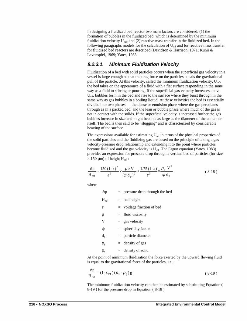
216 •••• NOXSO Process Integrated Environmental Control Model
In designing a fluidized bed reactor two main factors are considered: (1) theformation of bubbles in the fluidized bed, which is determined by the minimumfluidization velocity Umf, and (2) reactive mass transfer in the fluidized bed. In thefollowing paragraphs models for the calculation of Umf and for reactive mass transferfor fluidized bed reactors are described (Davidson & Harrison, 1971; Kunii &Levenspiel, 1969; Yates, 1983.
8.2.3.1. Minimum Fluidization VelocityFluidization of a bed with solid particles occurs when the superficial gas velocity in avessel is large enough so that the drag force on the particles equals the gravitationalpull of the particle. At this velocity, called the minimum fluidization velocity, Umf,the bed takes on the appearance of a fluid with a flat surface responding in the sameway as a fluid to stirring or pouring. If the superficial gas velocity increases aboveUmf, bubbles form in the bed and rise to the surface where they burst through in thesame way as gas bubbles in a boiling liquid. At these velocities the bed is essentiallydivided into two phases — the dense or emulsion phase where the gas percolatesthrough as in a packed bed, and the lean or bubble phase where much of the gas isnot in contact with the solids. If the superficial velocity is increased further the gasbubbles increase in size and might become as large as the diameter of the containeritself. The bed is then said to be "slugging" and is characterized by considerableheaving of the surface.
The expressions available for estimating Umf in terms of the physical properties ofthe solid particles and the fluidizing gas are based on the principle of taking a gasvelocity-pressure drop relationship and extending it to the point where particlesbecome fluidized and the gas velocity is Umf. The Ergun equation (Yates, 1983)provides an expression for pressure drop through a vertical bed of particles (for size> 150 µm) of height Hmf :
p
2
32p
3
2
mf d
V )-(1 1.75 +
)d (
V)-(1 150 =
H
p
ψρ
εε
ψµ
εε g×
××
∆( 8-18 )
where
p∆ = pressure drop through the bed
Hmf = bed height
ε = voidage fraction of bed
µ = fluid viscosity
V = gas velocity
ψ = sphericity factor
dp = particle diameter
ρg = density of gas
ρs = density of solid
At the point of minimum fluidization the force exerted by the upward flowing fluidis equal to the gravitational force of the particles, i.e.,
g ) - ( )-(1 = H
pmf
mfgs ρρε∆
( 8-19 )
The minimum fluidization velocity can then be estimated by substituting Equation (8-19 ) for the pressure drop in Equation ( 8-18 ):
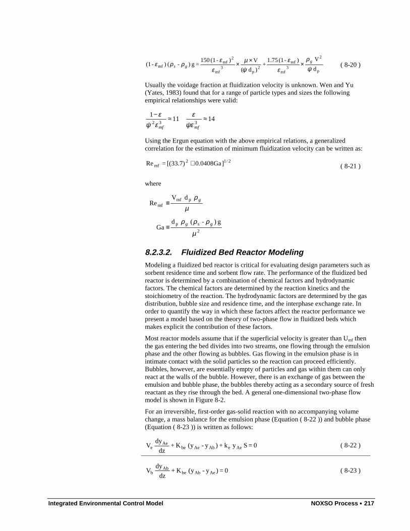
Integrated Environmental Control Model NOXSO Process •••• 217
p
2
3mf
mf2
p3
mf
2mf
mf d
V )-(1 1.75 +
)d (
V)-(1 150 = g ) - ( )-(1
ψρ
εε
ψµ
εε
ρρε ggs ××× ( 8-20 )
Usually the voidage fraction at fluidization velocity is unknown. Wen and Yu(Yates, 1983) found that for a range of particle types and sizes the followingempirical relationships were valid:
111
32≈−
mfεψε
143
≈mfψε
ε
Using the Ergun equation with the above empirical relations, a generalizedcorrelation for the estimation of minimum fluidization velocity can be written as:
2/12mf ]Ga0408.0[(33.7) = Re + ( 8-21 )
where
2
p
pmfmf
g ) - ( d Ga
d V Re
µ
ρρρ
µρ
gsg
g
≡
≡
8.2.3.2. Fluidized Bed Reactor ModelingModeling a fluidized bed reactor is critical for evaluating design parameters such assorbent residence time and sorbent flow rate. The performance of the fluidized bedreactor is determined by a combination of chemical factors and hydrodynamicfactors. The chemical factors are determined by the reaction kinetics and thestoichiometry of the reaction. The hydrodynamic factors are determined by the gasdistribution, bubble size and residence time, and the interphase exchange rate. Inorder to quantify the way in which these factors affect the reactor performance wepresent a model based on the theory of two-phase flow in fluidized beds whichmakes explicit the contribution of these factors.
Most reactor models assume that if the superficial velocity is greater than Umf thenthe gas entering the bed divides into two streams, one flowing through the emulsionphase and the other flowing as bubbles. Gas flowing in the emulsion phase is inintimate contact with the solid particles so the reaction can proceed efficiently.Bubbles, however, are essentially empty of particles and gas within them can onlyreact at the walls of the bubble. However, there is an exchange of gas between theemulsion and bubble phase, the bubbles thereby acting as a secondary source of freshreactant as they rise through the bed. A general one-dimensional two-phase flowmodel is shown in Figure 8-2.
For an irreversible, first-order gas-solid reaction with no accompanying volumechange, a mass balance for the emulsion phase (Equation ( 8-22 )) and bubble phase(Equation ( 8-23 )) is written as follows:
0 = S k + ) - ( K + AeeAbAebe yyydz
dy V Ae
e ( 8-22 )
0 = ) - ( K + AeAbbe yydz
dy V Ab
b ( 8-23 )
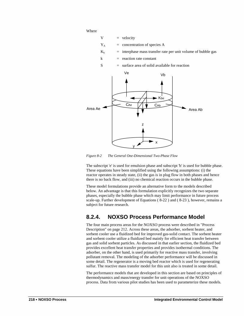
218 •••• NOXSO Process Integrated Environmental Control Model
Where
V = velocity
YA = concentration of species A
Kb = interphase mass transfer rate per unit volume of bubble gas
k = reaction rate constant
S = surface area of solid available for reaction
xy
z
Area AbArea Ae
Ve Vb
CAe CAb
Kbe
Figure 8-2 The General One-Dimensional Two-Phase Flow
The subscript 'e' is used for emulsion phase and subscript 'b' is used for bubble phase.These equations have been simplified using the following assumptions: (i) thereactor operates in steady state, (ii) the gas is in plug flow in both phases and hencethere is no back flow, and (iii) no chemical reaction occurs in the bubble phase.
These model formulations provide an alternative form to the models describedbelow. An advantage is that this formulation explicitly recognizes the two separatephases, especially the bubble phase which may limit performance in future processscale-up. Further development of Equations ( 8-22 ) and ( 8-23 ), however, remains asubject for future research.
8.2.4. NOXSO Process Performance ModelThe four main process areas for the NOXSO process were described in "ProcessDescription" on page 212. Across these areas, the adsorber, sorbent heater, andsorbent cooler use a fluidized bed for improved gas-solid contact. The sorbent heaterand sorbent cooler utilize a fluidized bed mainly for efficient heat transfer betweengas and solid sorbent particles. As discussed in that earlier section, the fluidized bedprovides excellent heat transfer properties and provides isothermal conditions. Theadsorber, on the other hand, is used primarily for reactive mass transfer, involvingpollutant removal. The modeling of the adsorber performance will be discussed insome detail. The regenerator is a moving bed reactor which is used for regeneratingsulfur. The reactive mass transfer model for this unit also is treated in some detail.
The performance models that are developed in this section are based on principles ofthermodynamics and mass/energy transfer for unit operations of the NOXSOprocess. Data from various pilot studies has been used to parameterize these models.
Integrated Environmental Control Model NOXSO Process •••• 219
8.2.4.1. Fluid Bed Adsorber ModelA mathematical model based on first principles has been developed by NOXSOCorporation for the design of future commercial installations (Ma and Haslbeck,1993). The reaction rate constants for SO2 and NOx sorption were derived using datafrom the process development unit (PDU), life cycle-test unit (LCTU), and proof ofconcept (POC) tests. The rate constants have been lumped to treat thehydrodynamics of the gas-solid contact and the reaction kinetics in one variable. Themain purpose of this model is to provide design equations for calculating key designparameters such as sorbent inventory and sorbent residence time for a desired levelof SO2 and NOx removal. We have rewritten the equations developed by NOXSOCorporation to provide explicit relations for the design variables. Since the equationsare quite detailed, and it is easy to get lost in the nomenclature, we first provide anoverview of the equations.
Equations ( 8-24 ) to ( 8-28 ) express the pollutant removal efficiency in terms of theoperating parameters of the fluidized bed (W, Fs) and physical constants (Ki, ρ, etc).The main objective here is to progressively rewrite the equations in terms ofvariables and functions which are readily measured and can be provided as inputs tothe model. Equation ( 8-29 ) and ( 8-30 ) provide a set of equations for removalefficiencies, operating parameters and physical constants. Equations ( 8-31 ) to (8-34 ) provide a set of relations for the physical constants determined fromexperimental data. Finally, Equations ( 8-35 ) and ( 8-36 ) provide the designequations for the operating parameters of the fluidized bed absorber.
The fluid bed mass balance in the vertical direction is derived using the followingassumptions: (i) there is no bubbling in the fluidized bed, (ii) the gas is in plug flow,(iii) the solids are in mixed flow, and (iv) SO2 and NOx absorption are first-orderreactions with respect to their concentrations. Therefore the mass balance is writtenas follows:
H )X-(1 y P Kn = )y - (y C V - iifioi0 iλρ ( 8-24 )
Notice that unlike Equation ( 8-22 ), the mass balance has been written for the totalbed by using a mean value for the concentration of gas species 'i'.
Defining the removal fraction as:
oi
fi
y
y-1 = iφ
Equation ( 8-24 ) can be rewritten as follows:
)X-(1 y
y P Kn
F
W =
oi
ii
gii λφ ( 8-25 )
When sorption takes place in the adsorber, both SO2 and NOx compete for activesites on the sorbent. A mass balance on the sorbent material in a mixed flow reactorresults in:
)X - (1 )y K+ y (K P W = )X - X( F 22110s ( 8-26 )
Combining Equations ( 8-25 ) and ( 8-26 ), the removal efficiency for the ith gasspecies can be rewritten as:
220 •••• NOXSO Process Integrated Environmental Control Model
)y K+ y (K P F
W + 1
1
y
y P K
F
EW =
2211s
oi
ii
g
iiφ
( 8-27 )
where
)X - (1n = E 0i iλ
Since the alumina substrate also adsorbs SO2 and NOx from the flue gas, thestochiometric ratio of reactant gas to active sorbent must include contributions fromboth sodium and alumina. In order to avoid having to make this distinction, anempirical relationship has been developed to calculate the stoichiometry as a ratio ofadsorber temperature:
a2
x
a1
2
T 075.0789.41
:NO
T 0052.03761.01
:SO
+−=
+=
λ
λ
For
For
( 8-28 )
where Ta is in degrees Celcius.
Since the gas flow in the fluidized bed is assumed to be plug flow and the reaction isfirst-order, y i can be taken as the logarithmic mean expressed in terms of theremoval efficiency as follows:
)-ln(1
-y = y oi
ii
i
φφ
Substituting for y i in Equation ( 8-27 ), the removal efficiencies can be written asfollows:
For SO2:
0K F
E
)1ln(
)1lny y )1ln(
1g
1
1 1
1
2
2 022011
01
=+
−−
+−−
o
s
A
AP
W
KKA
AP
F
W φφ
φφ(
φφ
( 8-29 )
For NOx:
0K F
E
)1ln(
)1lny y )1ln(
2g
2
2 2
2
1
1 011022
02
=+
−−
+−−
o
s
A
AP
W
KKA
AP
F
W φφ
φφ(
φφ
( 8-30 )
Note that since removal is a sorption reaction, the rate constant is proportional tosorbent surface area which has been introduced into the equations (refer to"Adsorber" on page 213). Equations ( 8-29 ) and ( 8-30 ) can be solvedsimultaneously for the removal efficiencies in terms of the following exogenouslyspecified variables :
1. The key operating parameters of the fluidized bed, i.e., sorbentresidence time (W/Fs) and sorbent inventory (W),
Integrated Environmental Control Model NOXSO Process •••• 221
2. Key inlet conditions including the mole fractions of SO2 and NOx (yoi)entering the adsorber, and the flue gas flow rate (Fg),
3. Key physical constants including the lumped kinetic constants (Ki), theavailable surface area (A/Ao), and the available unused sorbent capacity(Ei).
The physical constants have been determined by NOXSO Corporation usingexperimental data from the PDU, LCTU, and POC tests. In the following paragraphswe describe the parametrizations used for solving the above equations.
The sorbent's SO2 and NOx capacities are calculated as follows:
0
r112 A
A
3200
S - 0.8 +n = E :SOFor
λ ( 8-31 )
1
2r22x 3200
S - 0.8 +n = E :NOFor
λλλ
( 8-32 )
where
6000
n -
2300
n =n 2SiONa
Typically the sorbent contains 3.5-5% sodium and 6-7% silicon by weight.
The factor 0.8 in Equations ( 8-31 ) and ( 8-32 ) is the average sulfur content (% wt)of the regenerated sorbent in the PDU tests used as a reference for the aboveparameterization. The temperature dependent rate constants were derived byNOXSO Corporation by using PDU data along with Equations ( 8-29 ) and ( 8-30 )to solve for Ki at different temperatures. A least squares fit was used to obtain thefollowing relations:
273 + T
1840.2-exp 52.15 = K :SOFor
a12 ( 8-33 )
273 + T
912.14-exp 14.75 = K :NOFor
a2x ( 8-34 )
The available surface area A/Ao has a value of 0.6 based on PDU test data collectedafter sorbent surface area had stabilized.
For designing the adsorber, we need to estimate the operating parameters of thefluidized bed for given removal efficiencies for SO2 and NOx. The key parametersare the sorbent circulation rate, sorbent inventory, sorbent residence time andfluidized bed height. Equations ( 8-29 ) and ( 8-30 ) can be solved for sorbentinventory and sorbent circulation rate. Note that sorbent residence time also can becalculated from these two variables. The result is:
)b (
) ()b (
b
23323
1331223321
2332
1331
abab
bababababW
aba
baba
F
W
s
++−+
=
++
=
( 8-35 )
where
222 •••• NOXSO Process Integrated Environmental Control Model
a1 = ln(1 - 1φ )
b1 = (ln(1 - 2φ );
a2 = ;)-ln(1
)-ln(1
y K+ y K
A
AP
1
1
2
2022011
0
φ
φφ
φ
b2 = ;)-ln(1
)-ln(1
y K+ y K
A
AP
2
2
1
1011022
0
φ
φφ
φ
a3 =0
1g
1
A
AK P
F
E
b3 =0
2g
2
A
AK P
F
E
The height of the fluidized bed is calculated as follows:
aA
W = Hρ ( 8-36 )
The total sorbent inventory is calculated by adding the sorbent in the regenerator andthe solids heater and cooler as follows:
( ) ρSH/SCSH/SCOHCHsinv HA2 + t+ tF + W = S24
where ASH/SC is the cross-sectional area of the sorbent heater/cooler and HSH/SC is theheight of the sorbent. It has been assumed that the cross-sectional area for solidsheater and the solids cooler is the same. The total pressure drop in the fluidized bedis easily calculated by considering the total weight of sorbent that is fluidized by theflue gas, i.e.
aA
W = p∆
Sorbent attrition is caused by physical and thermal stresses that the sorbentexperiences as it is transported through the processing loop. These stresses canfracture the sorbent beads and erode the surface of the beads. Sorbent makeup is thenrequired to maintain a constant sorbent inventory. The attrition rate has beenmeasured experimentally at the pilot plant and is equivalent to 0.026% of theinventory per hour. The makeup sorbent is calculated as follows:
invsorbentmakeup SAR = m ×
where ARsorbent is the sorbent attrition rate.
Figure 8-3 and Figure 8-4 graph the sensitivity of the two design variables (W andW/Fs) to different SO2 and NOx removal efficiencies. These sensitivities are plottedfor a medium sulfur (2.6%S) Appalachian coal. The sorbent residence time (W/Fs)increases with the required SO2 and NOx removal (Figure 8-3). Similarly, the sorbentinventory (W) also increases with SO2 and NOx removal (Figure 8-4).

Integrated Environmental Control Model NOXSO Process •••• 223
sorb
ent r
esid
ence
tim
e (m
in.)
So2eff (fraction)0.8 0.85 0.9 0.95
25
30
35
40
45
50
Key Noxeff (fraction)0.70.750.80.85
Figure 8-3 Sorbent Residence Time in Adsorber (Medium Sulfur Appalachian Coal)
sorb
ent i
nv. i
n ad
sorb
er (
lb)
Noxeff (fraction)0.7 0.75 0.8 0.85
250K
300K
350K
400K
450K
Key So2eff (fraction)0.80.850.90.95
Figure 8-4 Sorbent Inventory in Adsorber (Medium Sulfur Appalachian Coal)
A promising alternative to the single-stage fluidized bed design described above is adesign featuring two fluidized beds in series. A schematic of the two-stage fluidizedbed absorber is shown in Figure 8-5. In the two-stage design, regenerated sorbententers a first stage fluidized bed, where the sorbent reacts with flue gas which hasalready passed through a second stage sorbent bed. The partially sulfated sorbentfrom the first bed then goes to a second bed, where it contacts inlet flue gas. Each ofthe two beds can have different bed heights and removal efficiencies. The overallremoval efficiency is given by:
( ) x2122 NO ,SO=i - 1 + = iiii φφφφ
where the subscripts 1,2 refer to the stage-1 and stage-2 fluidized beds. For each ofthe two beds, the general models given in Equation ( 8-35 ) and Equation ( 8-36 )apply. However, the input conditions for each bed is different. Since the output fluegas from the first stage enters the second stage, the SO2 and NOx concentrations are
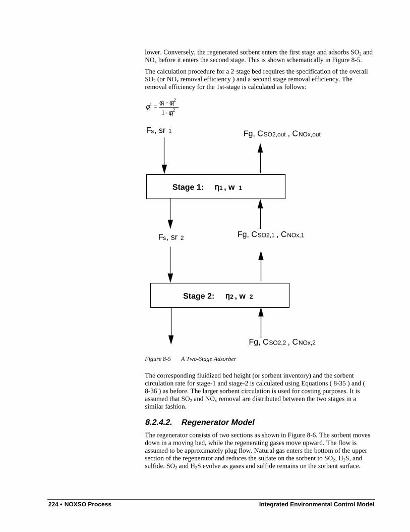
224 •••• NOXSO Process Integrated Environmental Control Model
lower. Conversely, the regenerated sorbent enters the first stage and adsorbs SO2 andNOx before it enters the second stage. This is shown schematically in Figure 8-5.
The calculation procedure for a 2-stage bed requires the specification of the overallSO2 (or NOx removal efficiency ) and a second stage removal efficiency. Theremoval efficiency for the 1st-stage is calculated as follows:
2
21
- 1
- =
i
iii φ
φφφ
����������������������������������������������������������������������������������������������������������������������������������������������������������������������������������������������������������������������������������������������������������������������������������������������������������������������������������������������������������������������������������������������������������������������������������������������������
����������������������������������������������������������������������������������������������������������������������������������������������������������������������������������������������������������������������������������������������������������������������������������������������������������������������������������������������������������������������������������������������������������������������������������������������������
Fs, sr 1
Fs, sr 2
Fg, CSO2,2 , CNOx,2
Fg, CSO2,1 , CNOx,1
Fg, CSO2,out , CNOx,out
Stage 1: ηηηη1 , w 1
Stage 2: ηηηη2 , w 2
Figure 8-5 A Two-Stage Adsorber
The corresponding fluidized bed height (or sorbent inventory) and the sorbentcirculation rate for stage-1 and stage-2 is calculated using Equations ( 8-35 ) and (8-36 ) as before. The larger sorbent circulation is used for costing purposes. It isassumed that SO2 and NOx removal are distributed between the two stages in asimilar fashion.
8.2.4.2. Regenerator ModelThe regenerator consists of two sections as shown in Figure 8-6. The sorbent movesdown in a moving bed, while the regenerating gases move upward. The flow isassumed to be approximately plug flow. Natural gas enters the bottom of the uppersection of the regenerator and reduces the sulfate on the sorbent to SO2, H2S, andsulfide. SO2 and H2S evolve as gases and sulfide remains on the sorbent surface.
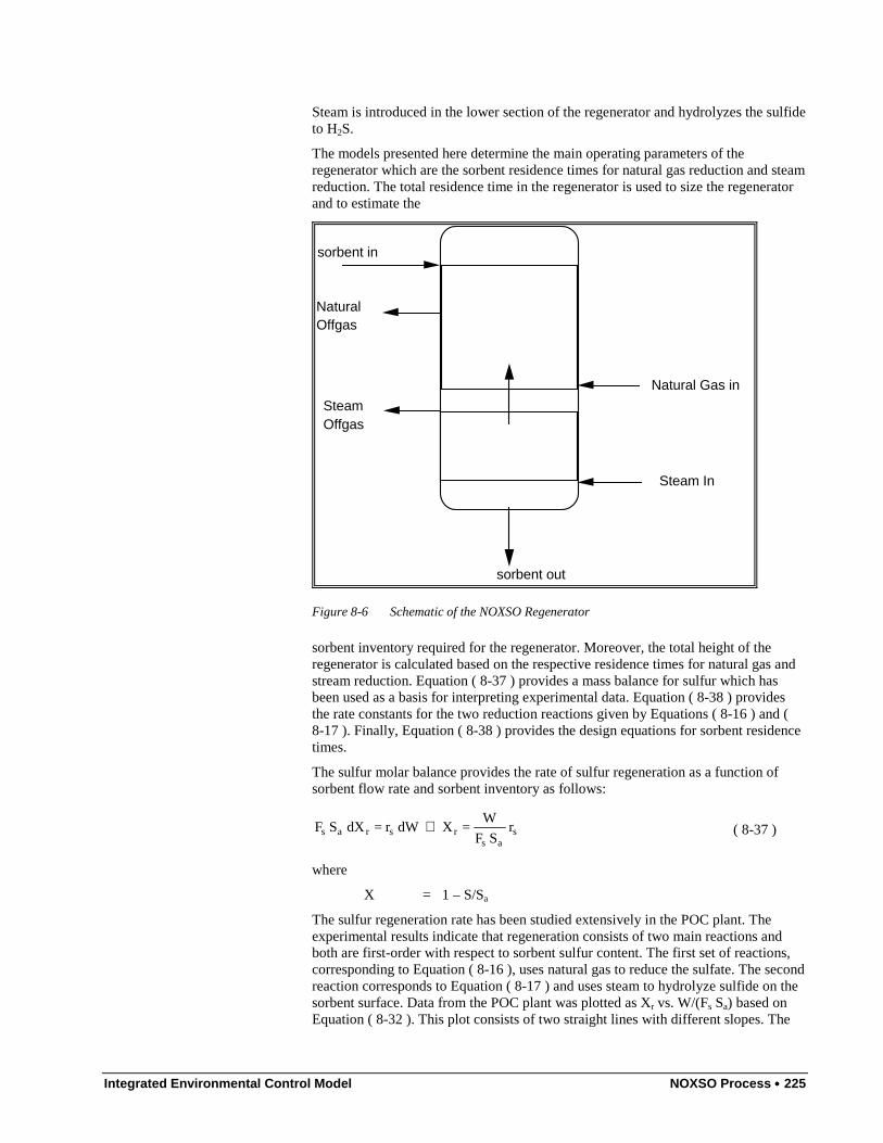
Integrated Environmental Control Model NOXSO Process •••• 225
Steam is introduced in the lower section of the regenerator and hydrolyzes the sulfideto H2S.
The models presented here determine the main operating parameters of theregenerator which are the sorbent residence times for natural gas reduction and steamreduction. The total residence time in the regenerator is used to size the regeneratorand to estimate the
Natural Gas in
Steam In
Steam Offgas
Natural Offgas
sorbent in
sorbent out
��������������������������������������������������������������������������������������������������������������������������������������������������������������������������������������������������������������������������������������������������������������������������������������������������������������������������������������������������������������������������������������������������������
����������������������������������������������������������������������������������������������������������������������������������������������������������������������������������������������������������������������������������������������������������
Figure 8-6 Schematic of the NOXSO Regenerator
sorbent inventory required for the regenerator. Moreover, the total height of theregenerator is calculated based on the respective residence times for natural gas andstream reduction. Equation ( 8-37 ) provides a mass balance for sulfur which hasbeen used as a basis for interpreting experimental data. Equation ( 8-38 ) providesthe rate constants for the two reduction reactions given by Equations ( 8-16 ) and (8-17 ). Finally, Equation ( 8-38 ) provides the design equations for sorbent residencetimes.
The sulfur molar balance provides the rate of sulfur regeneration as a function ofsorbent flow rate and sorbent inventory as follows:
sas
rsras r S F
W = X dW r = dX S F ⇒ ( 8-37 )
where
X = 1 – S/Sa
The sulfur regeneration rate has been studied extensively in the POC plant. Theexperimental results indicate that regeneration consists of two main reactions andboth are first-order with respect to sorbent sulfur content. The first set of reactions,corresponding to Equation ( 8-16 ), uses natural gas to reduce the sulfate. The secondreaction corresponds to Equation ( 8-17 ) and uses steam to hydrolyze sulfide on thesorbent surface. Data from the POC plant was plotted as Xr vs. W/(Fs Sa) based onEquation ( 8-32 ). This plot consists of two straight lines with different slopes. The
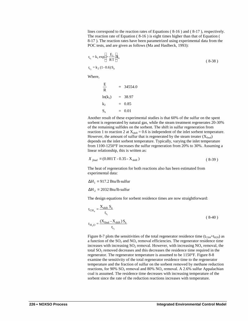
226 •••• NOXSO Process Integrated Environmental Control Model
lines correspond to the reaction rates of Equations ( 8-16 ) and ( 8-17 ), respectively.The reaction rate of Equation ( 8-16 ) is eight times higher than that of Equation (8-17 ). The reaction rates have been parametrized using experimental data from thePOC tests, and are given as follows (Ma and Haslbeck, 1993):
a2s
a1
1s
S 0.6)-(1 k = r
STR
Eexp k = r
2
1
−
( 8-38 )
Where,
R
E= 34554.0
ln(k1) = 38.97
k2 = 0.85
Sa = 0.01
Another result of these experimental studies is that 60% of the sulfur on the spentsorbent is regenerated by natural gas, while the steam treatment regenerates 20-30%of the remaining sulfides on the sorbent. The shift in sulfur regeneration fromreaction 1 to reaction 2 at Xshift = 0.6 is independent of the inlet sorbent temperature.However, the amount of sulfur that is regenerated by the steam treater (Xfinal)depends on the inlet sorbent temperature. Typically, varying the inlet temperaturefrom 1100-1250°F increases the sulfur regeneration from 20% to 30%. Assuming alinear relationship, this is written as:
)X-0.35-T 001.0( shift=finalX ( 8-39 )
The heat of regeneration for both reactions also has been estimated fromexperimental data:
sulfur Btu/lb 2032H
sulfur Btu/lb 2.917
2
1
=∆
=∆H
The design equations for sorbent residence times are now straightforward:
r
S )X-(X = t
r
S X = t
2
2
1
4
s
ashiftfinalOH
s
ashiftCH
( 8-40 )
Figure 8-7 plots the sensitivities of the total regenerator residence time (tCH4+tH20) asa function of the SO2 and NOx removal efficiencies. The regenerator residence timeincreases with increasing SO2 removal. However, with increasing NOx removal, thetotal SO2 removed decreases and this decreases the residence time required in theregenerator. The regenerator temperature is assumed to be 1150°F. Figure 8-8examine the sensitivity of the total regenerator residence time to the regeneratortemperature and the fraction of sulfur on the sorbent removed by methane reductionreactions, for 90% SO2 removal and 80% NOx removal. A 2.6% sulfur Appalachiancoal is assumed. The residence time decreases with increasing temperature of thesorbent since the rate of the reduction reactions increases with temperature.
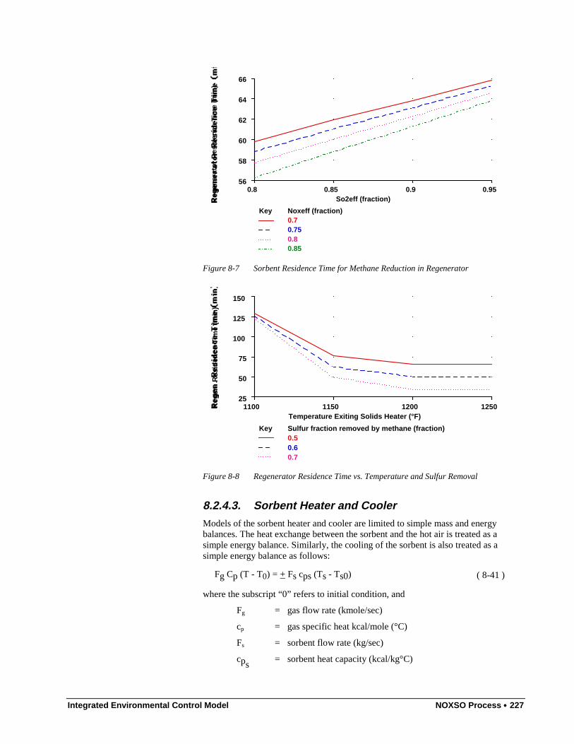
Integrated Environmental Control Model NOXSO Process •••• 227
Reg
ener
ator
Res
iden
ce T
ime
(min
)
So2eff (fraction)0.8 0.85 0.9 0.95
56
58
60
62
64
66
Key Noxeff (fraction)0.70.750.80.85
Figure 8-7 Sorbent Residence Time for Methane Reduction in Regenerator
Reg
en. R
esid
ence
Tim
e (m
in)
Temperature Exiting Solids Heater (°F)1100 1150 1200 1250
25
50
75
100
125
150
Key Sulfur fraction removed by methane (fraction)0.50.60.7
Figure 8-8 Regenerator Residence Time vs. Temperature and Sulfur Removal
8.2.4.3. Sorbent Heater and CoolerModels of the sorbent heater and cooler are limited to simple mass and energybalances. The heat exchange between the sorbent and the hot air is treated as asimple energy balance. Similarly, the cooling of the sorbent is also treated as asimple energy balance as follows:
�� � Fg Cp (T - T0) = + Fs cps (Ts - Ts0) ( 8-41 )
where the subscript “0” refers to initial condition, and
Fg = gas flow rate (kmole/sec)
cp = gas specific heat kcal/mole (°C)
Fs = sorbent flow rate (kg/sec)
cps= sorbent heat capacity (kcal/kg°C)
228 •••• NOXSO Process Integrated Environmental Control Model
Ts = sorbent temperature (°C)
The + signs are chosen depending on whether sorbent is being cooled or heated.These heat exchange models are used to calculate the energy requirement for sorbentheating and the related calculation of natural gas consumption.
The mass balance equations are used to evaluate the amount of NOx and SO2 that arerecycled to the boiler as part of the combustor gas. The NOx from the sorbent iscompletely desorbed in the sorbent heater and about 5-10% of the SO2 is desorbed.Since this extra amount of SO2 and NOx is recycled back to the flue gas, the absorberneeds to actually remove a large fraction of these species in order to achieve thesame levels of emissions as if there were no recycle. Mass balance equations areused to calculate the actual removal efficiencies for a desired level of emissions. Aschematic of the recycle loop is shown in Figure 8-9.
Boiler Adsorber
Solids Heater
mi M
ηn M
(1-R) ηN M
(1−ηo) mi
sorbent
i
i
i
Figure 8-9 Schematic of the Recycle Loop
The initial mass flow rate for each species (SO2, NOx) is denoted by mi and the massflow rate with recycle is denoted by Mi. The desired emission level of (1-ηo) mi isspecified with respect to mi and let us assume that the required removal efficiency isηo. Since the emission levels should not change with recycle, the actual removal
efficiency ηN required to achieve this is given by
( ) ( )OiNi -1 m = -1 M ηη ( 8-42 )
Moreover, from mass balance the recycle mass flow for species i (Mi) is related tooriginal mass flow rate mi as shown below:
( ) iNiii MR1m = M η−+ ( 8-43 )
Solving these equations for ηN we get
( ) ( )iO
ON
R1 -11 =
−− ηηη ( 8-44 )
where Ri is the recycle fraction for each species (94% for SO2 and 65% for NOx).

Integrated Environmental Control Model NOXSO Process •••• 229
8.2.4.4. A Numerical ExampleProvided here is a conceptual design of a commercial NOXSO plant of size 300 MWachieving 90% SO2 removal and 80% NOx removal. The coal used is a mediumsulfur Appalachian coal (2.6% sulfur, and 1.12% nitrogen). The design specificationsare:
Parameter Value
Plant Size 300 MW, 842 Kacfm (at 320°F)
Temp. of flue gas entering adsorber 320°F
SO2 removal requirement 90%
NOx removal requirement 80%
Inlet SO2 conc. (ηSO2) 1516 ppm (calculated by IECM)
Inlet NOx conc. (ηNOx) 400 ppm (calculated by IECM)
Sorbent Na2CO3 on γ-alumina spheres
Actual Removal Efficiencies
Since some NOx and SO2 are recycled back to the boiler, we need to calculate theactual absorber removal efficiencies required to achieve the desired design. This canbe calculated by a simple mass balance of SO2 and NOx around the power plant oncethe recycle fractions are known. Based on the current NOXSO design, these fractionsare 94% for SO2 and 65% for NOx. Thus,
( ) ( )
( ) ( ) 0.86=0.35)-(10.8)-(1-1
0.8=
R1 -11 =
0.905=0.06)-(10.9)-(1-1
0.9=
R1 -11 =
xx
x
22
2
NONO
NON,2
SOSO
SON,1
×−−
×−−
η
ηφ
η
ηφ
Adsorber
Physical parameters required for the calculations are first estimated. Substituting theadsorber temperature of 275°F in Equation ( 8-28 ) we estimate the stochiometricratios as follows:
0.19 =
0.93 =
2
1
λ
λ
Similarly, the temperature-dependent rate constants obtained from Equations ( 8-33 )and ( 8-34 ) are:
1-2
-11
sec) (atm 1.577 = K
sec) (atm 0.5734 = K
The sorbent capacities are calculated using Equations ( 8-31 ) and ( 8-32 ). Based onpilot plant data, the weight fraction of sodium in the sorbent is taken to be 3.8%,silicon content is about 5.2%, the sulfur content of regenerated sorbent is 0.25%, andthe available surface area fraction is 0.6. Thus,
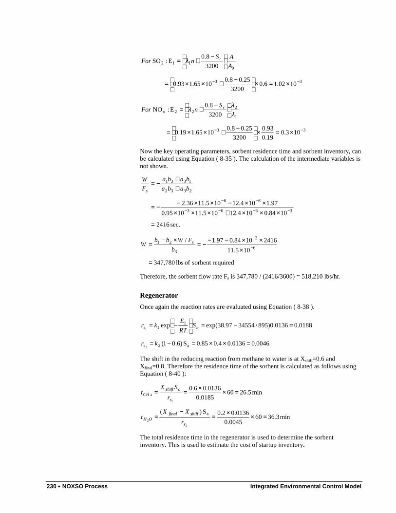
230 •••• NOXSO Process Integrated Environmental Control Model
33
0112
1002.16.03200
25.08.01065.193.0
3200
8.0E :SO
−− ×=×
−+××=
−
+=A
ASnFor rλ
33
1
222x
103.019.0
93.0
3200
25.08.01065.119.0
3200
8.0E :NO
−− ×=×
−+××=
−
+=λλλ rS
nFor
Now the key operating parameters, sorbent residence time and sorbent inventory, canbe calculated using Equation ( 8-35 ). The calculation of the intermediate variables isnot shown.
sec. 2416
1084.0104.12105.111095.0
97.1104.12105.1136.23663
66
2332
1331
=
×××+×××××−××−−=
++
−=
−−−−
−−
baba
baba
F
W
s
requiredsorbent of lbs 780,347
105.11
24161084.097.1/6
3
3
21
=
×××−−−=
×−= −
−
b
FWbbW s
Therefore, the sorbent flow rate Fs is 347,780 / (2416/3600) = 518,210 lbs/hr.
Regenerator
Once again the reaction rates are evaluated using Equation ( 8-38 ).
0046.00136.04.085.0S )6.01(
0188.00136.0)895/3455497.38exp( exp
a2
11
2
1
=××=−=
=−=
−=
kr
SRT
Ekr
s
as
The shift in the reducing reaction from methane to water is at Xshift=0.6 andXfinal=0.8. Therefore the residence time of the sorbent is calculated as follows usingEquation ( 8-40 ):
min3.36600045.0
0136.02.0S )(
min5.26600185.0
0136.06.0
2
2
1
4
a =××=−
=
=××==
s
shiftfinalOH
s
ashiftCH
r
XXt
r
SXt
The total residence time in the regenerator is used to determine the sorbentinventory. This is used to estimate the cost of startup inventory.
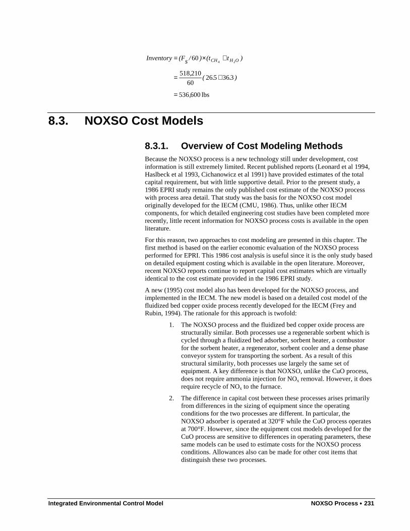
Integrated Environmental Control Model NOXSO Process •••• 231
lbs 600536
33652660
210518
6024
,
)..(,
)t(t)/s(FInventory OHCH
=
+=
+×=
8.3. NOXSO Cost Models
8.3.1. Overview of Cost Modeling MethodsBecause the NOXSO process is a new technology still under development, costinformation is still extremely limited. Recent published reports (Leonard et al 1994,Haslbeck et al 1993, Cichanowicz et al 1991) have provided estimates of the totalcapital requirement, but with little supportive detail. Prior to the present study, a1986 EPRI study remains the only published cost estimate of the NOXSO processwith process area detail. That study was the basis for the NOXSO cost modeloriginally developed for the IECM (CMU, 1986). Thus, unlike other IECMcomponents, for which detailed engineering cost studies have been completed morerecently, little recent information for NOXSO process costs is available in the openliterature.
For this reason, two approaches to cost modeling are presented in this chapter. Thefirst method is based on the earlier economic evaluation of the NOXSO processperformed for EPRI. This 1986 cost analysis is useful since it is the only study basedon detailed equipment costing which is available in the open literature. Moreover,recent NOXSO reports continue to report capital cost estimates which are virtuallyidentical to the cost estimate provided in the 1986 EPRI study.
A new (1995) cost model also has been developed for the NOXSO process, andimplemented in the IECM. The new model is based on a detailed cost model of thefluidized bed copper oxide process recently developed for the IECM (Frey andRubin, 1994). The rationale for this approach is twofold:
1. The NOXSO process and the fluidized bed copper oxide process arestructurally similar. Both processes use a regenerable sorbent which iscycled through a fluidized bed adsorber, sorbent heater, a combustorfor the sorbent heater, a regenerator, sorbent cooler and a dense phaseconveyor system for transporting the sorbent. As a result of thisstructural similarity, both processes use largely the same set ofequipment. A key difference is that NOXSO, unlike the CuO process,does not require ammonia injection for NOx removal. However, it doesrequire recycle of NOx to the furnace.
2. The difference in capital cost between these processes arises primarilyfrom differences in the sizing of equipment since the operatingconditions for the two processes are different. In particular, theNOXSO adsorber is operated at 320°F while the CuO process operatesat 700°F. However, since the equipment cost models developed for theCuO process are sensitive to differences in operating parameters, thesesame models can be used to estimate costs for the NOXSO processconditions. Allowances also can be made for other cost items thatdistinguish these two processes.
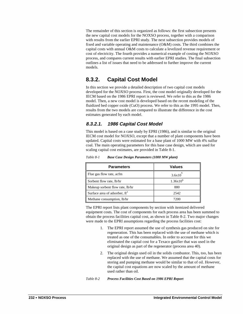
232 •••• NOXSO Process Integrated Environmental Control Model
The remainder of this section is organized as follows: the first subsection presentsthe new capital cost models for the NOXSO process, together with a comparisonwith results from the earlier EPRI study. The next subsection provides models offixed and variable operating and maintenance (O&M) costs. The third combines thecapital costs with annual O&M costs to calculate a levelized revenue requirement orcost of electricity. The fourth provides a numerical example of costing the NOXSOprocess, and compares current results with earlier EPRI studies. The final subsectionoutlines a list of issues that need to be addressed to further improve the currentmodels.
8.3.2. Capital Cost ModelIn this section we provide a detailed description of two capital cost modelsdeveloped for the NOXSO process. First, the cost model originally developed for theIECM based on the 1986 EPRI report is reviewed. We refer to this as the 1986model. Then, a new cost model is developed based on the recent modeling of thefluidized bed copper oxide (CuO) process. We refer to this as the 1995 model. Then,results from the two models are compared to illustrate the difference in the costestimates generated by each model.
8.3.2.1. 1986 Capital Cost ModelThis model is based on a case study by EPRI (1986), and is similar to the originalIECM cost model for NOXSO, except that a number of plant components have beenupdated. Capital costs were estimated for a base plant of 1000 MW with 4% sulfurcoal. The main operating parameters for this base case design, which are used forscaling capital cost estimates, are provided in Table 8-1.
Table 8-1 Base Case Design Parameters (1000 MW plant)
Parameters Values
Flue gas flow rate, acfm 3.6x10⁶
Sorbent flow rate, lb/hr 1.36x10⁶
Makeup sorbent flow rate, lb/hr 880
Surface area of adsorber, ft2 2542
Methane consumption, lb/hr 7200
The EPRI report lists plant components by section with itemized deliveredequipment costs. The cost of components for each process area has been summed toobtain the process facilities capital cost, as shown in Table 8-2. Two major changeswere made to the EPRI assumptions regarding the process facilities cost:
1. The EPRI report assumed the use of synthesis gas produced on site forregeneration. This has been replaced with the use of methane which istreated as one of the consumables. In order to account for this weeliminated the capital cost for a Texaco gasifier that was used in theoriginal design as part of the regenerator (process area 40).
2. The original design used oil in the solids combustor. This, too, has beenreplaced with the use of methane. We assumed that the capital costs forstoring and pumping methane would be similar to that of oil. However,the capital cost equations are now scaled by the amount of methaneused rather than oil.
Table 8-2 Process Facilities Cost Based on 1986 EPRI Report
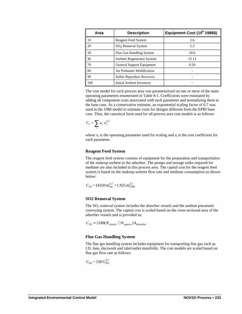
Integrated Environmental Control Model NOXSO Process •••• 233
Area Description Equipment Cost (10 6 1986$)
10 Reagent Feed System 2.6
20 SO2 Removal System 5.3
30 Flue Gas Handling System 20.6
40 Sorbent Regenerator System 15.13
70 General Support Equipment 0.29
80 Air Preheater Modification -
90 Sulfur Byproduct Recovery -
100 Initial Sorbent Inventory -
The cost model for each process area was parameterized on one or more of the mainoperating parameters enumerated in Table 8-1. Coefficients were estimated byadding all component costs associated with each parameter and normalizing them tothe base case. As a conservative estimate, an exponential scaling factor of 0.7 wasused in the 1986 model to estimate costs for designs different from the EPRI basecase. Thus, the canonical form used for all process area cost models is as follows:
∑i
0.7iii xa = C
where xi is the operating parameter used for scaling and ai is the cost coefficient foreach parameter.
Reagent Feed System
The reagent feed system consists of equipment for the preparation and transportationof the makeup sorbent to the adsorber. The pumps and storage tanks required formethane are also included in this process area. The capital cost for the reagent feedsystem is based on the makeup sorbent flow rate and methane consumption as shownbelow:
0.7CH4
0.7ms10 m 1.925 + m 14350 = C
SO2 Removal System
The SO2 removal system includes the absorber vessels and the sorbent pneumaticconveying system. The capital cost is scaled based on the cross sectional area of theadsorber vessels and is provided as:
absorbersparestowers ANNC )(218820 +=
Flue Gas Handling System
The flue gas handling system includes equipment for transporting flue gas such asI.D. fans, ductwork and inlet/outlet manifolds. The cost models are scaled based onflue gas flow rate as follows:
0.7FG30 G 530 = C
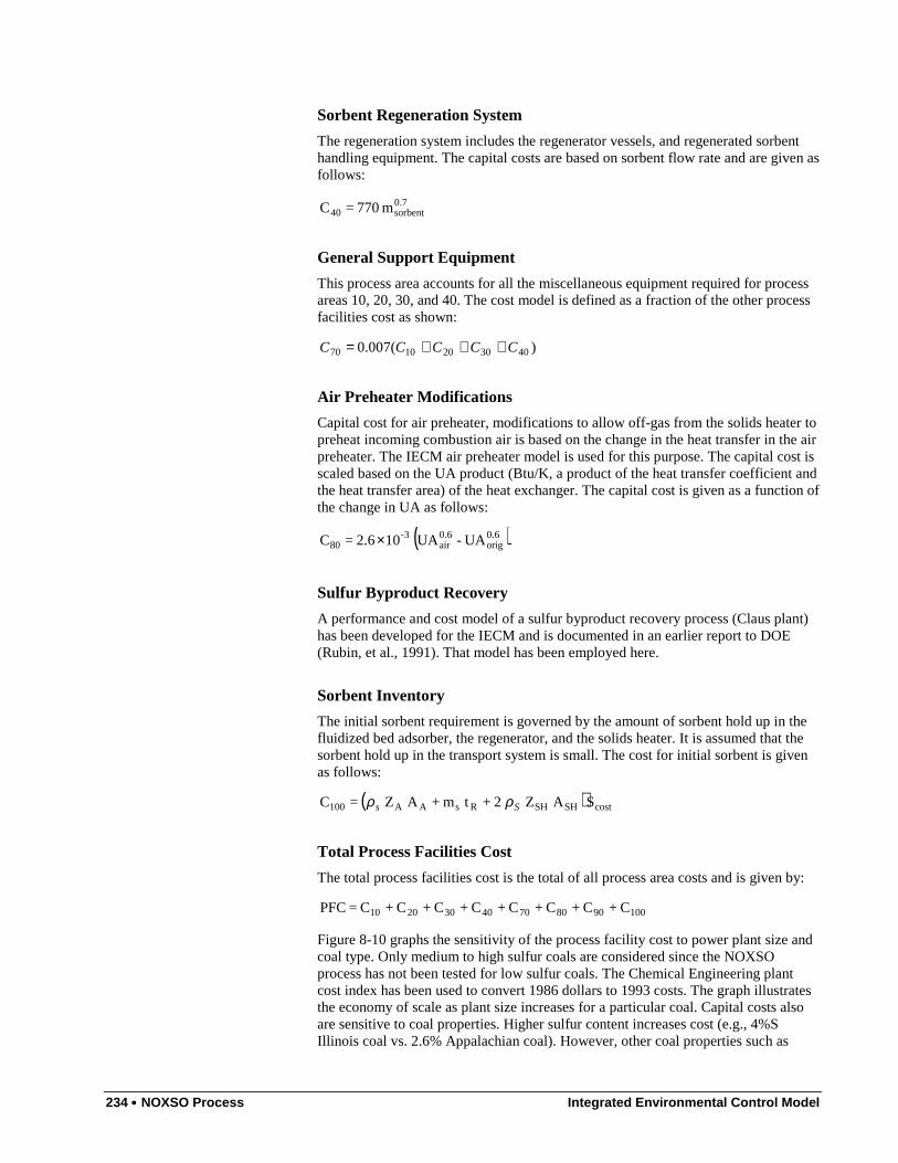
234 •••• NOXSO Process Integrated Environmental Control Model
Sorbent Regeneration System
The regeneration system includes the regenerator vessels, and regenerated sorbenthandling equipment. The capital costs are based on sorbent flow rate and are given asfollows:
0.7sorbent40 m 770 = C
General Support Equipment
This process area accounts for all the miscellaneous equipment required for processareas 10, 20, 30, and 40. The cost model is defined as a fraction of the other processfacilities cost as shown:
)(007.0 4030201070 CCCCC +++=
Air Preheater Modifications
Capital cost for air preheater, modifications to allow off-gas from the solids heater topreheat incoming combustion air is based on the change in the heat transfer in the airpreheater. The IECM air preheater model is used for this purpose. The capital cost isscaled based on the UA product (Btu/K, a product of the heat transfer coefficient andthe heat transfer area) of the heat exchanger. The capital cost is given as a function ofthe change in UA as follows:
( )0.6orig
0.6air
-380 UA- UA 102.6 = C ×
Sulfur Byproduct Recovery
A performance and cost model of a sulfur byproduct recovery process (Claus plant)has been developed for the IECM and is documented in an earlier report to DOE(Rubin, et al., 1991). That model has been employed here.
Sorbent Inventory
The initial sorbent requirement is governed by the amount of sorbent hold up in thefluidized bed adsorber, the regenerator, and the solids heater. It is assumed that thesorbent hold up in the transport system is small. The cost for initial sorbent is givenas follows:
( ) costSHSHRsAA100 S A Z 2 + tm + A Z = C Ss ρρ
Total Process Facilities Cost
The total process facilities cost is the total of all process area costs and is given by:
10090807040302010 C+C+C+C+C+C+C+C = PFC
Figure 8-10 graphs the sensitivity of the process facility cost to power plant size andcoal type. Only medium to high sulfur coals are considered since the NOXSOprocess has not been tested for low sulfur coals. The Chemical Engineering plantcost index has been used to convert 1986 dollars to 1993 costs. The graph illustratesthe economy of scale as plant size increases for a particular coal. Capital costs alsoare sensitive to coal properties. Higher sulfur content increases cost (e.g., 4%SIllinois coal vs. 2.6% Appalachian coal). However, other coal properties such as
Integrated Environmental Control Model NOXSO Process •••• 235
heating value that affect the flue gas volumetric flow also are important. Thus,although the North Dakota lignite has a lower sulfur content than the Appalachiancoal, its heating value also is substantially lower; this generates a larger gas volumeper MW of power produced, resulting in larger equipment sizes and higher cost. Allof these interactions are captured in the IECM.
Pro
cess
Fac
ilitie
s C
apita
l ($/
kW)
Gross Electrical Output (MWg)200 400 600 800 1000
75.0
100.0
125.0
150.0
175.0
200.0
Key Chosen CoalAppalachian Medium SulfurIllinois #6North Dakota Lignite
Figure 8-10 Total Process Facilities Cost (1993$) Based on the 1986 Model
8.3.2.2. 1995 Capital Cost ModelThe capital cost model presented in this section is based on a new cost modelrecently developed for the fluidized bed CuO process (CMU 1994). Appropriatechanges have been made to tailor the models to the NOXSO process. Compared tothe 1986 model, the new cost model is more highly disaggregated by process area.
Fluidized Bed Adsorbers
The process capital cost of the fluidized bed absorbers includes the absorber vessel,structural supports, dampers, isolation valves, refractory lining for the inside of theabsorber, ductwork, instrumentation and control, and installation costs.
The absorber vessels are refractory-lined carbon steel of minimum one-half inchthickness. Each absorber vessel may be approximated as a cylinder. The internaldiameter of the absorber vessel is determined based on the superficial gas velocityrequirement. The materials cost of the absorber is proportional to the surface area ofthe absorber vessel. The absorber vessel internal radius is given by:
towerss
FGA N V 60
G = r
π( 8-45 )
The diameter of the absorber vessel must be larger than this internal radius toaccommodate the thickness of refractory lining. The design basis developed by A. E.Roberts and Associates (AERA) for the copper oxide absorber includes a two-inchthick base or inner refractory covering the internal surface of the absorber vessel.This two-inch base or inner refractory lining also is assumed to be sufficient for theNOXSO process. The CuO process has an additional "hot base" refractory layerwhich is approximately six inches thick. However, since the adsorber temperature forthe NOXSO process is only 320°F (as compared to 700°F for the CuO process), the
236 •••• NOXSO Process Integrated Environmental Control Model
"hot base" is assumed to be unnecessary for the NOXSO vessel. Thus, the vesselinternal diameter is:
irAAV, t+ r = r ( 8-46 )
The surface area of the absorber vessel is approximated by the following equation forthe surface area of a cylinder:
( ) AAV,2
AV,A h r 2 + r 2 = SA ππ ( 8-47 )
The design height of the copper oxide absorber vessel is approximately 70 feet. Thetotal height of the absorber assembly is larger when flue gas outlet ductwork is takeninto consideration. The straight wall portion of the absorber vessel that is coveredwith refractory lining is approximately 35 feet.
The direct cost for the steel absorber vessel is estimated based on the ratio of surfaceareas referenced to a base case design. The copper oxide design is predicated on aflue gas volumetric flow rate of approximately 500,000 scfm at 705°F and asuperficial gas velocity of 4.5 ft/sec. For this case, the approximate surface area ofthe absorber vessel is 24,875 ft2. The base cost estimate is $1,434,000 (in 1993dollars) for a single absorber vessel of this size. Therefore, the direct cost model forthe cost of the NOXSO steel absorber vessel is given by:
PCI 1993875,24N 1434 total,
PCISAC A
VA
=
where the smaller surface area for the NOXSO process is calculated from Equations( 8-45 ) to ( 8-47 ). Typically, there will be two 50% capacity absorber vessels withno spares.
The cost of refractory is given by the refractory surface area, required to cover thesides of the absorber vessel, and a unit cost for refractory per square foot:
costtowersSA,ARA, R N h r 2 = C π
In 1993 dollars, the unit cost of the total of 8 inches of refractory required for theabsorber was approximately $55/ft2.
Each absorber requires structural supports. In the copper oxide design, these areestimated at $100,000 per vessel. The structural support is assumed here to havesome economy of scale with respect to size. A six-tenths scaling rule traditionallyused in the process technology and chemical engineering literature is assumed:
PCI 1993875,24N 100
6.0
total,PCISA
C ASA
=
The surface area of the absorber vessel is used as a surrogate variable for the size ofthe absorber system and, hence, the proportional size of the structural supports.
The Costs for flue gas ductwork, flue gas isolation valves, and dampers are assumedto be proportional to the flue gas volumetric flow rate. Moreover, economies of scaleare assumed. In the absence of more detailed information, the following direct costmodel was adapted based on the copper oxide study:
PCI 1993
PCI
N 101.1
G N 300 = C
6.0
towers6FG
totaldA,
×

Integrated Environmental Control Model NOXSO Process •••• 237
In this model, the cost of ductwork, isolation valves, and dampers is estimated for asingle absorber vessel, and is multiplied by the total number of absorber vessels. Thetotal direct cost for the absorber process area is then given by:
)CCC(C )f +(1 = C dA,SA,RA,VA,aic,A +++
where fic,a is an installation cost factor for the absorber process area. A default valueof 0.45 is suggested for the CuO process and adopted as well for the NOXSOprocess.
In addition to these direct costs, there is a cost associated with using a new induceddraft fan to overcome the pressure drop of the flue gas in the adsorber. The fanefficiency is typically 85 percent. The cost of the ID fan differential is:
PCI 1993
PCI
4600
EC N 180 = C
6.0ID
tA,ID
Regenerator
The regenerator cost model assumes a carbon steel cylindrical vessel sized toaccommodate sorbent storage for a specified sorbent residence time. The base casecopper oxide design has a regenerator with a sorbent hold-up volume of 8,800 ft3.The regenerator design features a 28 foot straight wall height. Here, it is assumedthat the straight wall height is held fixed, and the radius is adjusted to accommodatevarious residence times. Usually, columns that are higher than 28-30 feet requirebuildings with high roofs which increase construction costs. The required regeneratorradius for the NOXSO process is therefore given by:
SR,towers
RRs,R h N 60
tm = r
πρ s
The total height of the regenerator is the straight wall height plus inlet and outletclearances for gas flows. These clearances add approximately 17 feet to the straightwall height. The inside of the regenerator vessel walls are covered with two layers ofrefractory totaling 8 inches in thickness. Therefore, the steel vessel diameter is:
irRRV, t+ r = r
The surface area of the regenerator vessel is approximated by the surface area of acylinder:
( ) RRV,2
RV,R h r 2 + r 2 = SA ππ
For the copper oxide process, the regenerator has an equivalent overall height of 78feet and a radius of 10 feet, yielding a surface area of 5530 ft2. The direct cost of theNOXSO regenerator vessel is then estimated as:
PCI 1993
PCI
N 5305
SA N 475 = C
6.0
tR,
RtotaldR,
The additional direct cost of refractory is given by:
costtR,SR,RRR, R N h r 2 = C π
238 •••• NOXSO Process Integrated Environmental Control Model
Each regenerator requires structural supports. In the base case design, this cost isestimated at $42,500 per vessel. The structural support is assumed here to have someeconomy of scale with respect to size. A six-tenths scaling rule again is assumed:
PCI 1993
PCI
N 5305
SA N 42.5 = C
6.0
tR,
RtotalsR,
The surface area of the absorber vessel is used as a surrogate variable for the size ofthe regenerator system and, hence, the proportional size of the structural supports.
The costs for ductwork, isolation valves, and dampers are assumed to be proportionalto the regenerator off-gas volume flow rate. Moreover, economies of scale areassumed. In the base case analysis, approximately 626 lbmole/hour of off-gas isevolved from each of the two copper oxide regenerator vessels. At 900°F, thevolumetric flow rate is 21,900 ft3/min. Thus, in the absence of more detailedinformation, the following direct cost model was developed:
PCI 1993
PCI
N 266
G N 350 = C
6.0
tR,
FGtotaldR,
In this model, the cost of ductwork, isolation valves, and dampers is estimated for asingle absorber vessel, then multiplied by the total number of absorber vessels.
A methane feed system, a booster compressor and motor are required for the inletmethane to overcome the pressure drop through the regenerator. The boostercompressor cost is assumed to be proportional to the methane flow rate. Againscaling costs from the copper oxide model gives:
PCI 1993
PCI
N 871
M N 350 = C
6.0
tR,
CH4R,totalCH4R,
The total direct cost for the absorber process area is given by:
)CCCC(C )f +(1 = C CH4R,dR,SR,RR,VR,Ric,R ++++
where fic,R is an installation cost factor for the absorber process area. A default valueof 0.45 again is suggested.
Solids Heater
The solids heater is assumed to be a carbon steel cylindrical vessel. For the copperoxide process, AERA has designed a solids heater with an internal radius of 10 feetand a height of 50 feet. The side walls of the heater are lined with refractorymaterial. The internal diameter of the solids heater is proportional to the mass flowof sorbent entering the vessel. The vessel contains two sorbent beds in which hotcombustion gases from a methane combustor contact the sorbent in counter-currentflow. Thus, for fixed bed heights in each stage, the solids heater internal radius varieswith the sorbent mass flow rate as follows:
tSH
SHSHs
N
tm
,
,
000,400
The inside of the solids heater vessel walls are covered with two layers of refractorytotaling 8 inches in thickness. Therefore, the steel vessel diameter is:
Integrated Environmental Control Model NOXSO Process •••• 239
irSHSHV, t+ r = r
The surface area of the solids heater vessel is approximated by the surface area of acylinder. Thus, for a single vessel, the surface area is:
( ) SHSHV,2
SHV,SH h r 2 + r 2 = SA ππ
In the base case, the solids heater has an equivalent overall height of 50 feet and aninternal radius of 10 feet. Scaling results for the copper oxide process, the direct costof the NOXSO regenerator vessel is:
PCI 1993
PCI
N 0604
SA N 360 = C
6.0
tSH,
SHtotalVSH,
The additional direct cost of refractory is given by:
costtSH,SSH,SHVSH, R N h r 2 = C π
Each solids heater requires structural supports. In the copper oxide design, these areestimated at $72,500 per vessel. The structural support is assumed here to have someeconomy of scale with respect to size. A six-tenths scaling rule gives:
PCI 1993
PCI
N 0604
SA N 72.5 = C
6.0
tSH,
SHtSH,sSH,
The surface area of the solids heater vessel is used as a surrogate variable for the sizeof the NOXSO solids heater system and, hence, the proportional size of the structuralsupports.
The costs for ductwork, isolation valves, dampers, booster fans and motors areassumed to be proportional to the solids heater exit gas volumetric flow rate. Again,economies of scale are assumed. In the copper oxide process, approximately 6,500lbmole/hour of gas exits the solids heater at 830°F. Thus, the following direct costmodel was developed:
PCI 1993
PCI
N 4676
G N 608 = C
6.0
tSH,
offSH,totaldSH,
In this model, the cost of ductwork, isolation valves, dampers, booster fans, andbooster fan motors is estimated for a single solids heater vessel, and multiplied bythe total number of absorber vessels.
The total direct cost for the solids heater is:
)CCC(C )f +(1 = C dSH,SSH,rR,VSH,SHic,SH +++
where fic,R is an installation cost factor for the absorber process area. A default valueof 0.45 is suggested.
Sorbent Transport System
A dense phase pneumatic transport system is employed to transport sorbent from theregenerator outlet to the absorber inlet. The transport system includes valves,compressors, piping, filters, and surge bins. The dense phase transport system was

240 •••• NOXSO Process Integrated Environmental Control Model
sized for a sorbent circulation rate of 1,000,000 lb/hr. The total cost for this systemfor the copper oxide process is $6,580,000. The cost of the NOXSO transport systemis assumed to be proportional to the sorbent circulation rate. Thus, the equipmentcost for the dense phase transport system is:
PCI 1993
PCI
000,000,1
m 6580 = C
6.0sorbent
eST,
In addition, a sorbent storage silo is required. The cost of these silos is proportionalto the sorbent circulation rate and the sorbent attrition rate, which determine thesorbent make-up rate. The nominal sorbent makeup rate is 500 lb/hr in the base casedesign. Therefore, the cost of the storage silos with air locks is:
PCI 1993
PCI
500
m 330 = C
6.0makeup
sST,
The total direct cost for the sorbent transport system is:
)C(C )f +(1 = C sST,eST,STic,ST +
where fic,ST is an installation cost factor for the solids transport process area. Adefault value of 0.45 is suggested.
Solids Heater Combustor
The cost of the combustor for the solids heater is assumed to be proportional to themethane requirement: Scaling results for the copper oxide combustor gives:
PCI 1993
PCI
225
m )f +(1 330 = C
6.0SHCH4,
cSH,ic,sSH,
where fic,SH,c is an installation cost factor for the solids heater combustor processarea. A default value of 0.45 is suggested.
Byproduct Recovery
A performance and cost model (CBy) of a byproduct sulfur recovery plant has beendeveloped previously (Rubin et al., 1991). This model has been adapted for theNOXSO process.
Air Preheater Modifications
The NOXSO process produces off-gas from the solids heater at temperatures ofabout 610°F. This can be used to preheat the combustion air going into the boiler.The cost of air preheater modifications (CAPH) to allow this was shown previously.
Initial Sorbent Inventory
The initial sorbent requirement is governed primarily by the amount of sorbent holdup in the fluidized bed absorber, the regenerator, and the solids heater. It is assumedthat the quantity of sorbent hold up in the transport system is small by comparison.The cost for initial sorbent fill is therefore:
( ) costSHSHRsAAIS, S A Z 2 + tm + A Z = C Ss ρρ
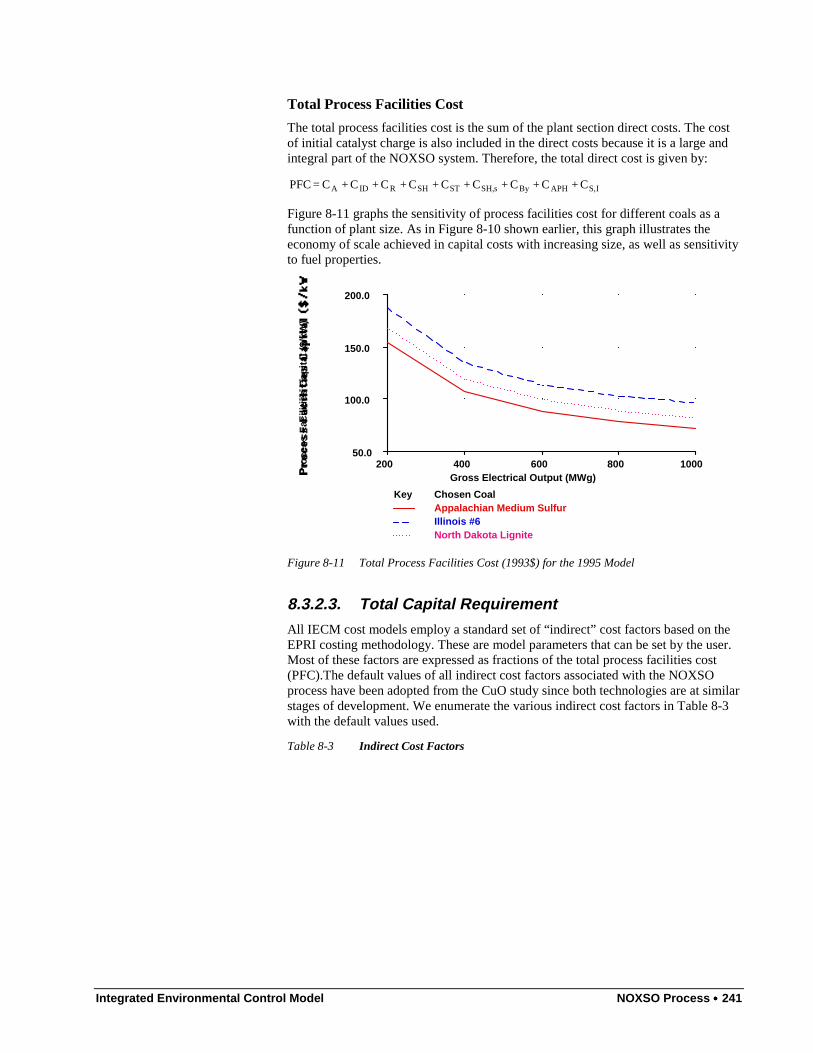
Integrated Environmental Control Model NOXSO Process •••• 241
Total Process Facilities Cost
The total process facilities cost is the sum of the plant section direct costs. The costof initial catalyst charge is also included in the direct costs because it is a large andintegral part of the NOXSO system. Therefore, the total direct cost is given by:
IS,APHBysSH,STSHRIDA C+C+C+C+C+C+C+C+C = PFC
Figure 8-11 graphs the sensitivity of process facilities cost for different coals as afunction of plant size. As in Figure 8-10 shown earlier, this graph illustrates theeconomy of scale achieved in capital costs with increasing size, as well as sensitivityto fuel properties.
Pro
cess
Fac
ilitie
s C
apita
l ($/
kW)
Gross Electrical Output (MWg)200 400 600 800 1000
50.0
100.0
150.0
200.0
Key Chosen CoalAppalachian Medium SulfurIllinois #6North Dakota Lignite
Figure 8-11 Total Process Facilities Cost (1993$) for the 1995 Model
8.3.2.3. Total Capital RequirementAll IECM cost models employ a standard set of “indirect” cost factors based on theEPRI costing methodology. These are model parameters that can be set by the user.Most of these factors are expressed as fractions of the total process facilities cost(PFC).The default values of all indirect cost factors associated with the NOXSOprocess have been adopted from the CuO study since both technologies are at similarstages of development. We enumerate the various indirect cost factors in Table 8-3with the default values used.
Table 8-3 Indirect Cost Factors
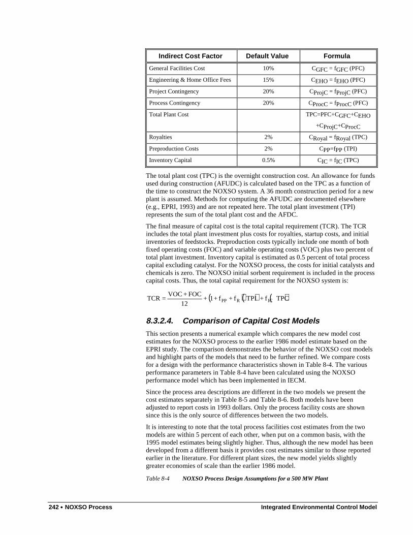
242 •••• NOXSO Process Integrated Environmental Control Model
Indirect Cost Factor Default Value Formula
General Facilities Cost 10% CGFC = fGFC (PFC)
Engineering & Home Office Fees 15% CEHO = fEHO (PFC)
Project Contingency 20% CProjC = fProjC (PFC)
Process Contingency 20% CProcC = fProcC (PFC)
Total Plant Cost TPC=PFC+CGFC+CEHO
+CProjC+CProcC
Royalties 2% CRoyal = fRoyal (TPC)
Preproduction Costs 2% CPP=fPP (TPI)
Inventory Capital 0.5% CIC = fIC (TPC)
The total plant cost (TPC) is the overnight construction cost. An allowance for fundsused during construction (AFUDC) is calculated based on the TPC as a function ofthe time to construct the NOXSO system. A 36 month construction period for a newplant is assumed. Methods for computing the AFUDC are documented elsewhere(e.g., EPRI, 1993) and are not repeated here. The total plant investment (TPI)represents the sum of the total plant cost and the AFDC.
The final measure of capital cost is the total capital requirement (TCR). The TCRincludes the total plant investment plus costs for royalties, startup costs, and initialinventories of feedstocks. Preproduction costs typically include one month of bothfixed operating costs (FOC) and variable operating costs (VOC) plus two percent oftotal plant investment. Inventory capital is estimated as 0.5 percent of total processcapital excluding catalyst. For the NOXSO process, the costs for initial catalysts andchemicals is zero. The NOXSO initial sorbent requirement is included in the processcapital costs. Thus, the total capital requirement for the NOXSO system is:
( ) ( ) ( )TPC f + TPI f +f+1 + 12
FOC+VOC = TCR ICRPP
8.3.2.4. Comparison of Capital Cost ModelsThis section presents a numerical example which compares the new model costestimates for the NOXSO process to the earlier 1986 model estimate based on theEPRI study. The comparison demonstrates the behavior of the NOXSO cost modelsand highlight parts of the models that need to be further refined. We compare costsfor a design with the performance characteristics shown in Table 8-4. The variousperformance parameters in Table 8-4 have been calculated using the NOXSOperformance model which has been implemented in IECM.
Since the process area descriptions are different in the two models we present thecost estimates separately in Table 8-5 and Table 8-6. Both models have beenadjusted to report costs in 1993 dollars. Only the process facility costs are shownsince this is the only source of differences between the two models.
It is interesting to note that the total process facilities cost estimates from the twomodels are within 5 percent of each other, when put on a common basis, with the1995 model estimates being slightly higher. Thus, although the new model has beendeveloped from a different basis it provides cost estimates similar to those reportedearlier in the literature. For different plant sizes, the new model yields slightlygreater economies of scale than the earlier 1986 model.
Table 8-4 NOXSO Process Design Assumptions for a 500 MW Plant
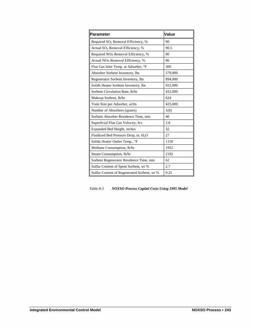
Integrated Environmental Control Model NOXSO Process •••• 243
Parameter Value
Required SO2 Removal Efficiency, % 90
Actual SO2 Removal Efficiency, % 90.5
Required NOx Removal Efficiency, % 80
Actual NOx Removal Efficiency, % 86
Flue Gas Inlet Temp. at Adsorber, °F 300
Absorber Sorbent Inventory, lbs 579,000
Regenerator Sorbent Inventory, lbs 894,000
Solids Heater Sorbent Inventory, lbs 931,000
Sorbent Circulation Rate, lb/hr 432,000
Makeup Sorbent, lb/hr 624
Train Size per Adsorber, acfm 425,000
Number of Absorbers (spares) 1(0)
Sorbent Absorber Residence Time, min 40
Superficial Flue Gas Velocity, ft/s 2.8
Expanded Bed Height, inches 32
Fluidized Bed Pressure Drop, in. H2O 27
Solids Heater Outlet Temp., °F 1150
Methane Consumption, lb/hr 1952
Steam Consumption, lb/hr 2192
Sorbent Regenerator Residence Time, min 62
Sulfur Content of Spent Sorbent, wt % 2.7
Sulfur Content of Regenerated Sorbent, wt % 0.25
Table 8-5 NOXSO Process Capital Costs Using 1995 Model
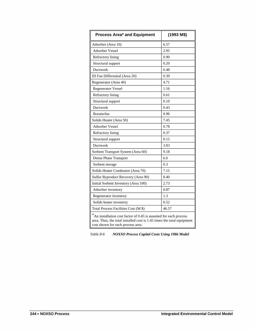
244 •••• NOXSO Process Integrated Environmental Control Model
Process Area* and Equipment (1993 M$)
Adsorber (Area 10) 6.57
Adsorber Vessel 2.95
Refractory lining 0.90
Structural support 0.20
Ductwork 0.48
ID Fan Differential (Area 20) 0.39
Regenerator (Area 40) 4.71
Regenerator Vessel 1.16
Refractory lining 0.61
Structural support 0.10
Ductwork 0.43
Boosterfan 0.96
Solids Heater (Area 50) 7.45
Adsorber Vessel 0.78
Refractory lining 0.37
Structural support 0.15
Ductwork 3.83
Sorbent Transport System (Area 60) 9.18
Dense Phase Transport 6.0
Sorbent storage 0.3
Solids Heater Combustor (Area 70) 7.15
Sulfur Byproduct Recovery (Area 90) 8.40
Initial Sorbent Inventory (Area 100) 2.73
Adsorber inventory 0.87
Regenerator inventory 1.3
Solids heater inventory 0.52
Total Process Facilities Cost (M $) 46.57
*An installation cost factor of 0.45 is assumed for each processarea. Thus, the total installed cost is 1.45 times the total equipmentcost shown for each process area.
Table 8-6 NOXSO Process Capital Costs Using 1986 Model
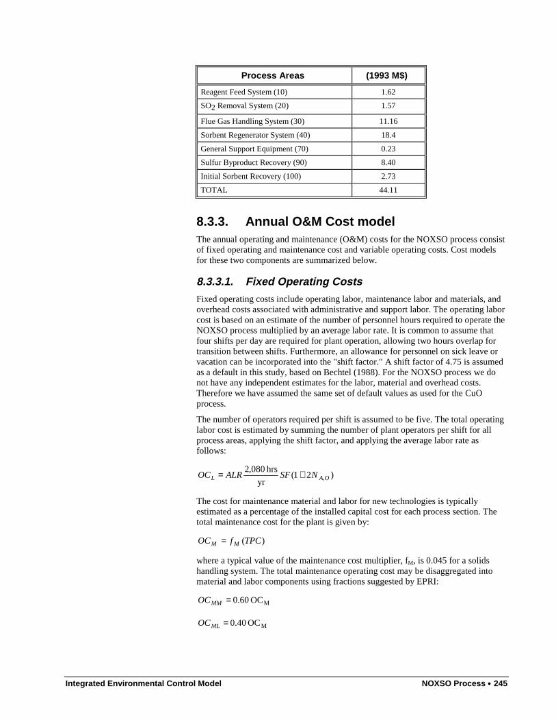
Integrated Environmental Control Model NOXSO Process •••• 245
Process Areas (1993 M$)
Reagent Feed System (10) 1.62
SO2 Removal System (20) 1.57
Flue Gas Handling System (30) 11.16
Sorbent Regenerator System (40) 18.4
General Support Equipment (70) 0.23
Sulfur Byproduct Recovery (90) 8.40
Initial Sorbent Recovery (100) 2.73
TOTAL 44.11
8.3.3. Annual O&M Cost modelThe annual operating and maintenance (O&M) costs for the NOXSO process consistof fixed operating and maintenance cost and variable operating costs. Cost modelsfor these two components are summarized below.
8.3.3.1. Fixed Operating CostsFixed operating costs include operating labor, maintenance labor and materials, andoverhead costs associated with administrative and support labor. The operating laborcost is based on an estimate of the number of personnel hours required to operate theNOXSO process multiplied by an average labor rate. It is common to assume thatfour shifts per day are required for plant operation, allowing two hours overlap fortransition between shifts. Furthermore, an allowance for personnel on sick leave orvacation can be incorporated into the "shift factor." A shift factor of 4.75 is assumedas a default in this study, based on Bechtel (1988). For the NOXSO process we donot have any independent estimates for the labor, material and overhead costs.Therefore we have assumed the same set of default values as used for the CuOprocess.
The number of operators required per shift is assumed to be five. The total operatinglabor cost is estimated by summing the number of plant operators per shift for allprocess areas, applying the shift factor, and applying the average labor rate asfollows:
)21(yr
hrs 080,2,OAL NSFALROC +=
The cost for maintenance material and labor for new technologies is typicallyestimated as a percentage of the installed capital cost for each process section. Thetotal maintenance cost for the plant is given by:
)(TPCfOC MM =
where a typical value of the maintenance cost multiplier, fM, is 0.045 for a solidshandling system. The total maintenance operating cost may be disaggregated intomaterial and labor components using fractions suggested by EPRI:
MOC 60.0=MMOC
MOC 40.0=MLOC
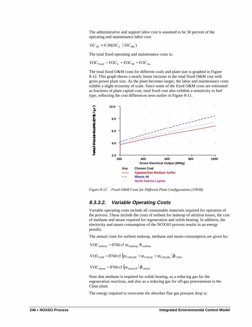
246 •••• NOXSO Process Integrated Environmental Control Model
The administrative and support labor cost is assumed to be 30 percent of theoperating and maintenance labor cost:
)(30.0 MLLAS OCOCOC +=
The total fixed operating and maintenance costs is:
FOC+ FOC+ FOC = FOC AsMLTotal
The total fixed O&M costs for different coals and plant size is graphed in Figure8-12. This graph shows a nearly linear increase in the total fixed O&M cost withgross power plant size. As the plant becomes larger, the labor and maintenance costsexhibit a slight economy of scale. Since some of the fixed O&M costs are estimatedas fractions of plant capital cost, total fixed cost also exhibits a sensitivity to fueltype, reflecting the cost differences seen earlier in Figure 8-11.
Tot
al F
ixed
Cos
ts (
M$/
yr)
Gross Electrical Output (MWg)200 400 600 800 1000
2.0
4.0
6.0
8.0
10.0
Key Chosen CoalAppalachian Medium SulfurIllinois #6North Dakota Lignite
Figure 8-12 Fixed O&M Costs for Different Plant Configurations (1993$)
8.3.3.2. Variable Operating CostsVariable operating costs include all consumable materials required for operation ofthe process. These include the costs of sorbent for makeup of attrition losses, the costof methane and steam required for regeneration and solids heating. In addition, theelectricity and steam consumption of the NOXSO process results in an energypenalty.
The annual costs for sorbent makeup, methane and steam consumption are given by:
sorbentmakeupsorbent R m cf 8760 = VOC
( ) CH4ByCH4,RCH4,SHCH4,CH4 R m + m + m cf 8760 = VOC
( ) steamRsteam,steam R m cf 8760 = VOC
Note that methane is required for solids heating, as a reducing gas for theregeneration reactions, and also as a reducing gas for off-gas pretreatment in theClaus plant.
The energy required to overcome the absorber flue gas pressure drop is:
Integrated Environmental Control Model NOXSO Process •••• 247
8512
N P G = EC OA,AFG
IDfanη
∆
Additional energy requirements for sorbent transport and for overcoming thepressure drop in the solids heater are calculated as follows:
sorbent6sorbent m (lb/hr) 101.36
(kW) 1795 = EC
×
8512
P G = EC
AHOffgasAH
fanη∆
where the pressure drop ∆PAH in the solids heater is typically about 4 inches of H2O,and the fan efficiency is in the range of 50-85%, combining the three equationsabove yields the overall electrical energy operating cost:
( ) ElecIDAHsorbentElec R ECECEC cf 8760 = VOC ++
Note that in the IECM the internal cost of electricity either can be specified by theuser or calculated by the model based on generating costs for a new power plant.
Finally, the variable operating costs also include a byproduct credit for the sale ofelemental sulfur produced by the Claus plant. The amount of this credit is given by:
SR SO2,
ByBy R 2000
M 32 cf 8760 = VOC
η
Summarizing the above terms, the total variable operating cost is:
ByElec
steamCH4sorbentTotal
VOC - VOC+
VOC+ VOC+ VOC = VOC
The total variable cost for different coals and plant sizes is graphed in Figure 8-13.As with fixed O&M cost, the total variable cost also increases in a nearly linearlyfashion with plant size, reflecting larger input and output flows of plant materials andenergy requirements. In this case, however, there is a slight upward curvature,indicating slightly higher variable costs with increasing plant size. This is primarilydue to nonlinearities that result in higher sorbent requirements and attrition losseswith larger vessel sizes. Overall, however, this is not a significant factor affectingeconomics of scale.
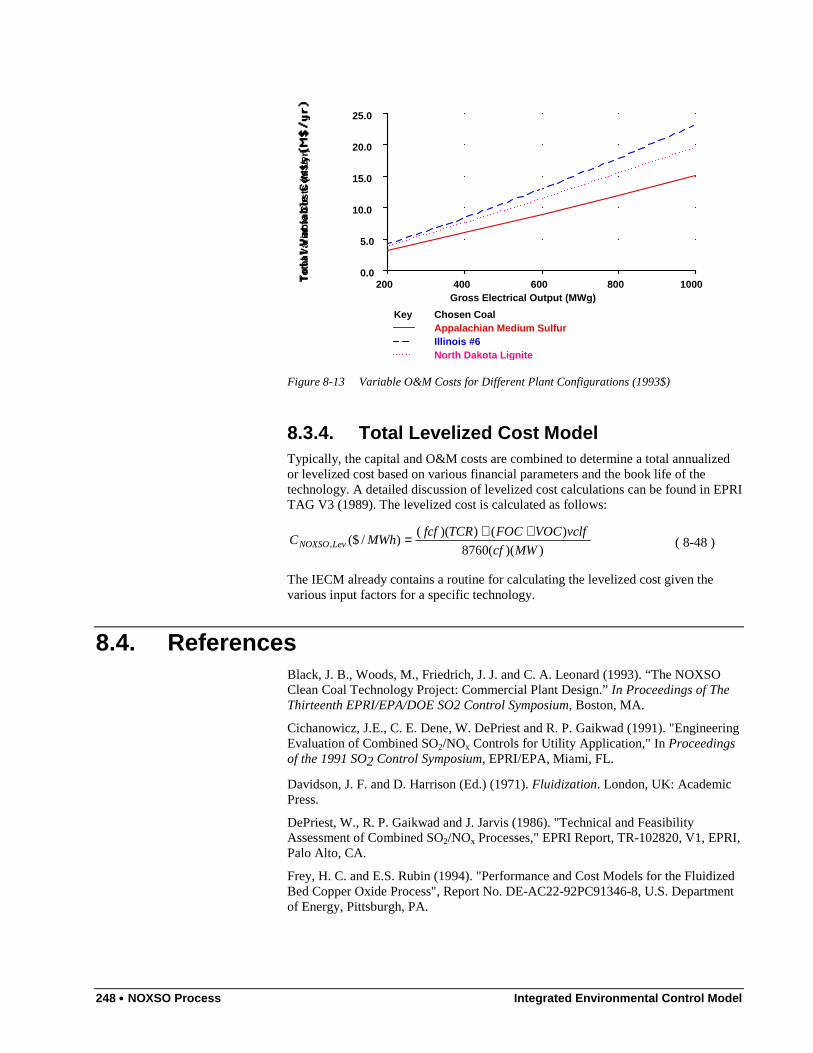
248 •••• NOXSO Process Integrated Environmental Control Model
Tot
al V
aria
ble
Cos
ts (
M$/
yr)
Gross Electrical Output (MWg)200 400 600 800 1000
0.0
5.0
10.0
15.0
20.0
25.0
Key Chosen CoalAppalachian Medium SulfurIllinois #6North Dakota Li gnite
Figure 8-13 Variable O&M Costs for Different Plant Configurations (1993$)
8.3.4. Total Levelized Cost ModelTypically, the capital and O&M costs are combined to determine a total annualizedor levelized cost based on various financial parameters and the book life of thetechnology. A detailed discussion of levelized cost calculations can be found in EPRITAG V3 (1989). The levelized cost is calculated as follows:
))((8760
)())(()/($,
MWcf
vclfVOCFOCTCRfcfMWhC LevNOXSO
++= ( 8-48 )
The IECM already contains a routine for calculating the levelized cost given thevarious input factors for a specific technology.
8.4. ReferencesBlack, J. B., Woods, M., Friedrich, J. J. and C. A. Leonard (1993). “The NOXSOClean Coal Technology Project: Commercial Plant Design.” In Proceedings of TheThirteenth EPRI/EPA/DOE SO2 Control Symposium, Boston, MA.
Cichanowicz, J.E., C. E. Dene, W. DePriest and R. P. Gaikwad (1991). "EngineeringEvaluation of Combined SO2/NOx Controls for Utility Application," In Proceedingsof the 1991 SO2 Control Symposium, EPRI/EPA, Miami, FL.
Davidson, J. F. and D. Harrison (Ed.) (1971). Fluidization. London, UK: AcademicPress.
DePriest, W., R. P. Gaikwad and J. Jarvis (1986). "Technical and FeasibilityAssessment of Combined SO2/NOx Processes," EPRI Report, TR-102820, V1, EPRI,Palo Alto, CA.
Frey, H. C. and E.S. Rubin (1994). "Performance and Cost Models for the FluidizedBed Copper Oxide Process", Report No. DE-AC22-92PC91346-8, U.S. Departmentof Energy, Pittsburgh, PA.
Integrated Environmental Control Model NOXSO Process •••• 249
Haslbeck, J. L. and L.G. Neal (1985). “The NOXSO Process Development: AnUpdate.” In Ninth EPA/EPRI Symposium on Flue Gas Desulfurization, Cincinnati,OH.
Haslbeck, J.L., M.C. Woods, W.T. Ma, S.M. Harkins and J.B. Black (1993)."NOXSO SO2/NOx Flue Gas Treatment: Proof-of-Concept Test", In Proceedings of1993 SO2 Control Symposium, EPRI/DOE, Boston, MA.
Kunii, D. and O. Levenspiel (1969). Fluidization Engineering. New York: Wiley.
Leonard, C.A., J.L. Haslbeck, J.J. Friedrich and M.C. Woods (1994). "NOXSOEconomics," Technical Report prepared by NOXSO Corp., Unpublished Manuscript.
Ma, W. T., J.L. Haslbeck, et al. (1993). “Proof-of-Concept Testing of the AdvancedNOXSO Flue Gas Cleanup Process,” Report of Contract No. DE-AC22-89PC88889,U.S. Department of Energy, Pittsburgh, PA.
Rubin, E.S., J.S. Salmento, H. C. Frey, A. Abu-Baker and M. Berkenpas (1991).“Modeling of Integrated Environmental Control Systems for Coal-Fired PowerPlants,” Report DE-AC22-87PC79864, U.S. Department of Energy, Pittsburgh, PA.
Yates, J. G. (1983). Fundamentals of Fluidized-Bed Chemical Processes. Boston,MA: Butterworths.
Yeh, J. T., Drummond, C. J., Haslbeck, J. L. and L.G. Neal (1987). “The NOXSOProcess: Simultaneous Removal of SO2 and NOx from Flue Gas.” In Proceedings ofSpring National Meeting of the AIChE, Houston, TX.
Yeh, J. T., Ma, W. T., Pennline, H. W., Haslbeck, J. L. and F.N. Gromicko (1990).Integrated Testing of the NOXSO Process: Simultaneous Removal of SO2 and NOx
from Flue Gas. In Proceedings of AIChE Spring National Meeting, Orlando, FL.

250 •••• Appendix Integrated Environmental Control Model
9. Appendix
9.1. Introduction to “Integrated Environmental ControlModeling of Coal-Fired Power Systems”
This appendix contains the text, figures and tables from a technical paper deliveredat the Air & Waste Management Association meeting held in the summer of 1996.The paper was published in their journal the following year.† The paper is providedas an example of the power, applicability, and ease of the IECM. For a completecopy of the actual paper, please refer to the journal directly.
9.2. AbstractThe capability to estimate the performance and costs of advanced environmentalcontrol systems for coal-fired power plants is critical to a variety of planning andanalysis requirements faced by utilities, regulators, researchers and analysts in thepublic and private sectors. This paper describes a computer model developed for theU.S. Department of Energy (USDOE) to provide an up-to-date capability foranalyzing a variety of pre-combustion, combustion, and post-combustion options inan integrated framework. A unique feature of the model allows performance andcosts of integrated environmental control concepts to be modeled probabilistically asa means of characterizing uncertainties and risks. Examples are presented of modelapplications comparing conventional and advanced emission control designs. Themagnitude of technology risks associated with advanced technologies now underdevelopment are seen to vary markedly across applications. In general, however,integrated environmental control concepts show significant potential for more cost-effective methods of emissions control.
9.3. IntroductionOver the past two decades, new environmental control requirements havesubstantially altered the design of fossil fuel power plants, especially for coal-firedplants, which supply nearly 60 percent of U.S. electricity demand. The developmentof environmental regulations has been a largely piecemeal approach, focused on oneenvironmental medium at a time (air, water, solids), with a changing set of standards
† Rubin, E.S.; Kalagnanam, J.R.; Frey, H.C.; Berkenpas, M.B. “Integrated Environmental Control Modeling of Coal-Fired Power Systems,” Journal of the Air & Waste Management Association. 1997, 11:47, 1180-1188.
Integrated Environmental Control Model Appendix •••• 251
and requirements for individual pollutants. In turn, new technologies have beenadded to address each new problem or requirement that arises. The result of thispiecemeal approach has been high cost and often unsatisfactory performance ofenvironmental control technology.
More recently, the concept of integrated environmental control has emerged as animportant new paradigm for the design of electric power systems. This concept has anumber of dimensions. One involves the integration of pollution control functionscurrently carried out in separate devices or unit operations, for example thereplacement of separate processes for SO2 and NOx control by a single system forcombined removal of both pollutants. Integration also includes the consideration ofmethods to control air pollutants, water pollutants and solid wastes simultaneously,as opposed to separate solutions for each environmental medium. Finally, theconcept of integrated control includes an examination of environmental controloptions at different stages of the fuel cycle, for example, control methods that can beapplied before, during and after the combustion process, as opposed to a focus onone area alone.
This paper describes a computerized modeling framework developed for the U.S.Department of Energy (USDOE) to provide the capability to analyze theperformance and cost of integrated emission control concepts for coal-fired electricpower plants. This capability is critical to a variety of planning, analysis, and designrequirements faced by utility companies, regulators, researchers and analysts. Aunique capability of the model is that it allows performance and costs to becharacterized probabilistically, using Monte Carlo methods to quantify performanceand cost uncertainties and risks. The Integrated Environmental Control Model(IECM) is intended to support a variety of applications related to technologyassessment, process design, and research management. Examples of questions thatcan be addressed with the model include the following:
• What uncertainties most affect the overall performance and costs of aparticular technology?
• What are the key design trade-offs for a particular process?
• What are the potential payoffs and risks of advanced processes vis-a-vis conventional technology?
• Which technologies appear most promising for further processdevelopment?
• What conditions or markets favor the selection of one system design (ortechnology) over another?
• How can technical and/or economic uncertainties be reduced mosteffectively through further research and development?
9.4. ImplicationsEstimating the performance and cost of advanced technologies still underdevelopment is one of the most difficult tasks facing decision makers, policy analystsand research managers in the public and private sectors. The modeling frameworkdescribed in this paper offers an approach to help minimize technological risks byexplicitly considering uncertainties in the development of performance and costestimates for integrated environmental control options applicable to modern coal-based power generation systems.
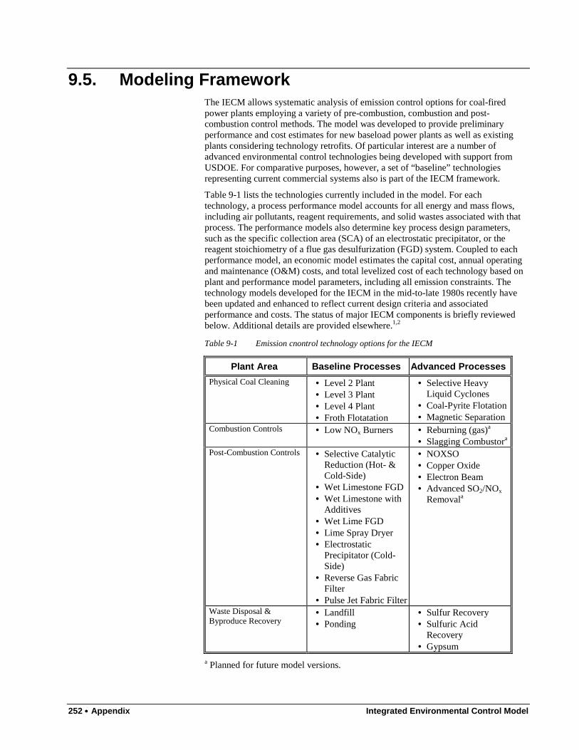
252 •••• Appendix Integrated Environmental Control Model
9.5. Modeling FrameworkThe IECM allows systematic analysis of emission control options for coal-firedpower plants employing a variety of pre-combustion, combustion and post-combustion control methods. The model was developed to provide preliminaryperformance and cost estimates for new baseload power plants as well as existingplants considering technology retrofits. Of particular interest are a number ofadvanced environmental control technologies being developed with support fromUSDOE. For comparative purposes, however, a set of “baseline” technologiesrepresenting current commercial systems also is part of the IECM framework.
Table 9-1 lists the technologies currently included in the model. For eachtechnology, a process performance model accounts for all energy and mass flows,including air pollutants, reagent requirements, and solid wastes associated with thatprocess. The performance models also determine key process design parameters,such as the specific collection area (SCA) of an electrostatic precipitator, or thereagent stoichiometry of a flue gas desulfurization (FGD) system. Coupled to eachperformance model, an economic model estimates the capital cost, annual operatingand maintenance (O&M) costs, and total levelized cost of each technology based onplant and performance model parameters, including all emission constraints. Thetechnology models developed for the IECM in the mid-to-late 1980s recently havebeen updated and enhanced to reflect current design criteria and associatedperformance and costs. The status of major IECM components is briefly reviewedbelow. Additional details are provided elsewhere.1,2
Table 9-1 Emission cnontrol technology options for the IECM
Plant Area Baseline Processes Advanced Processes
Physical Coal Cleaning • Level 2 Plant• Level 3 Plant• Level 4 Plant• Froth Flotatation
• Selective HeavyLiquid Cyclones
• Coal-Pyrite Flotation• Magnetic Separation
Combustion Controls • Low NOx Burners • Reburning (gas)a
• Slagging Combustora
Post-Combustion Controls • Selective CatalyticReduction (Hot- &Cold-Side)
• Wet Limestone FGD• Wet Limestone with
Additives• Wet Lime FGD• Lime Spray Dryer• Electrostatic
Precipitator (Cold-Side)
• Reverse Gas FabricFilter
• Pulse Jet Fabric Filter
• NOXSO• Copper Oxide• Electron Beam• Advanced SO2/NOx
Removala
Waste Disposal &Byproduce Recovery
• Landfill• Ponding
• Sulfur Recovery• Sulfuric Acid
Recovery• Gypsum
a Planned for future model versions.
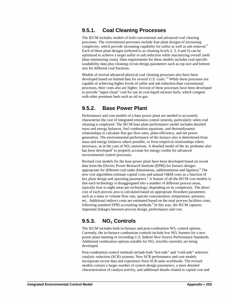
Integrated Environmental Control Model Appendix •••• 253
9.5.1. Coal Cleaning ProcessesThe IECM includes models of both conventional and advanced coal cleaningprocesses. The conventional processes include four plant designs of increasingcomplexity, which provide increasing capability for sulfur as well as ash removal.3
Each of these plant designs (referred to as cleaning levels 2, 3, 4 and 5) can beoptimized to achieve a target sulfur or ash reduction while maximizing overall yield(thus minimizing costs). Data requirements for these models includes coal-specificwashability data plus cleaning circuit design parameters such as top size and bottomsize for different coal fractions.
Models of several advanced physical coal cleaning processes also have beendeveloped based on limited data for several U.S. coals.1,2 While these processes arecapable of achieving higher levels of sulfur and ash reduction than conventionalprocesses, their costs also are higher. Several of these processes have been developedto provide “super-clean” coal for use in coal-liquid mixture fuels, which competewith other premium fuels such as oil or gas.
9.5.2. Base Power PlantPerformance and cost models of a base power plant are needed to accuratelycharacterize the cost of integrated emission control systems, particularly when coalcleaning is employed. The IECM base plant performance model includes detailedmass and energy balances, fuel combustion equations, and thermodynamicrelationships to calculate flue gas flow rates, plant efficiency, and net powergeneration. The environmental performance of the furnace also is determined frommass and energy balances where possible, or from empirical relationships wherenecessary, as in the case of NOx emissions. A detailed model of the air preheater alsohas been developed2 to properly account for energy credits for advancedenvironmental control processes.
Revised cost models for the base power plant have been developed based on recentdata from the Electric Power Research Institute (EPRI) for furnace designsappropriate for different coal ranks (bituminous, subbituminous and lignites).4 Thenew cost algorithms estimate capital costs and annual O&M costs as a function ofkey plant design and operating parameters.5 A feature of all the IECM cost models isthat each technology is disaggregated into a number of different process areas,typically four to eight areas per technology, depending on its complexity. The directcost of each process area is calculated based on appropriate flowsheet parameterssuch as a mass or volume flow rate, species concentration, temperature, pressure,etc.. Additional indirect costs are estimated based on the total process facilities costs,following standard EPRI accounting methods.4 In this way, the IECM capturesimportant linkages between process design, performance and cost.
9.5.3. NOx ControlsThe IECM includes both in-furnace and post-combustion NOx control options.Currently, the in-furnace combustion controls include low NOx burners for a newpower plant meeting or exceeding U.S. federal New Source Performance Standards.Additional combustion options suitable for NOx retrofits currently are beingdeveloped.
Post-combustion control methods include both “hot-side” and “cold-side” selectivecatalytic reduction (SCR) systems. New SCR performance and cost modelsincorporate recent data and experience from SCR units worldwide. The revisedmodels contain a larger number of system design parameters, a more detailedcharacterization of catalyst activity, and additional details related to capital cost and
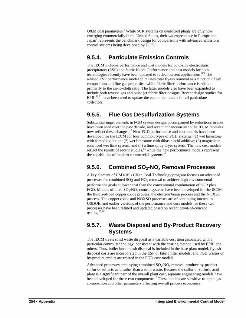
254 •••• Appendix Integrated Environmental Control Model
O&M cost parameters.6 While SCR systems on coal-fired plants are only nowemerging commercially in the United States, their widespread use in Europe andJapan7 represents the benchmark design for comparisons with advanced emissionscontrol systems being developed by DOE.
9.5.4. Particulate Emission ControlsThe IECM includes performance and cost models for cold-side electrostaticprecipitators (ESP) and fabric filters. Performance and cost models for bothtechnologies recently have been updated to reflect current applications.8,9 Therevised ESP performance model calculates total flyash removal as a function of ashcomposition and flue gas properties, while fabric filter performance is relatedprimarily to the air-to-cloth ratio. The latter models also have been expanded toinclude both reverse gas and pulse jet fabric filter designs. Recent design studies forEPRI10,11 have been used to update the economic models for all particulatecollectors.
9.5.5. Flue Gas Desulfurization SystemsSubstantial improvements in FGD system design, accompanied by reductions in cost,have been seen over the past decade, and recent enhancements to the IECM modulesnow reflect these changes.12 New FGD performance and cost models have beendeveloped for the IECM for four common types of FGD systems: (1) wet limestonewith forced oxidation; (2) wet limestone with dibasic acid additive; (3) magnesium-enhanced wet lime system; and (4) a lime spray dryer system. The new cost modelsreflect the results of recent studies,13 while the new performance models representthe capabilities of modern commercial systems.14
9.5.6. Combined SO 2-NOx Removal ProcessesA key element of USDOE’s Clean Coal Technology program focuses on advancedprocesses for combined SO2 and NOx removal to achieve high environmentalperformance goals at lower cost than the conventional combination of SCR plusFGD. Models of three SO2/NOx control systems have been developed for the IECM:the fluidized-bed copper oxide process, the electron beam process and the NOXSOprocess. The copper oxide and NOXSO processes are of continuing interest toUSDOE, and earlier versions of the performance and cost models for these twoprocesses have been refined and updated based on recent proof-of-concepttesting.15,16
9.5.7. Waste Disposal and By-Product RecoverySystems
The IECM treats solid waste disposal as a variable cost item associated with aparticular control technology, consistent with the costing method used by EPRI andothers. Thus, boiler bottom ash disposal is included in the base plant model, fly ashdisposal costs are incorporated in the ESP or fabric filter models, and FGD wastes orby-product credits are treated in the FGD cost models.
Advanced processes employing combined SO2/NOx removal produce by-productsulfur or sulfuric acid rather than a solid waste. Because the sulfur or sulfuric acidplant is a significant part of the overall plant cost, separate engineering models havebeen developed for these two components.2 These models are sensitive to input gascomposition and other parameters affecting overall process economics.
Integrated Environmental Control Model Appendix •••• 255
9.6. Probabilistic CapabilityA unique feature of the IECM is its ability to characterize input parameters andoutput results probabilistically, in contrast to conventional deterministic (pointestimate) models. This method of analysis offers a number of important advantagesover the traditional approach of examining uncertainties only through sensitivityanalysis. Probabilistic analysis allows the interactive effects of variations in manydifferent parameters to be considered simultaneously, in contrast to sensitivityanalysis where only one or two parameters at a time are varied, with all otherparameters held constant. In addition, probabilistic analysis provides quantitativeinsights about the likelihood of various outcomes, and the probability that one resultmay be more significant than another. This type of information on technical andeconomic risks often is of greater value than simple bounding or “worst case”analyses obtained from sensitivity studies, which contain no information on thelikelihood of worst case occurrences.
The ability to perform probabilistic analysis comes from the use of a software systemwhich uses a non-procedural modeling environment designed to facilitate modelbuilding and probabilistic analysis.17 In addition to a number of standard probabilitydistributions (e.g., normal, lognormal, uniform, chance), the IECM canaccommodate any arbitrarily specified distribution for input parameters. Given aspecified set of input uncertainties, the resulting uncertainties induced in modeloutputs are calculated using median Latin Hypercube sampling, an efficient variantof Monte Carlo simulation. Results typically are displayed in the form of acumulative probability distribution showing the likelihood of reaching or exceedingvarious levels of a particular parameter of interest (e.g., efficiency, emissions orcost).
9.7. Model ApplicationsThe IECM recently has been modified to allow estimation of retrofit costs as well asnew plant costs. A series of user-specified retrofit factors may be applied at theprocess area level for a particular system to estimate the higher costs of retrofitfacilities. To use the model, a graphical interface has been developed which providesan extremely user-friendly mode of operation.18
Here we present results illustrating the capabilities of the IECM to evaluate andcompare conventional and advanced emissions control systems. The base case plantshown in Figure 9-1 achieves 90% SO2 removal employing a wet limestone FGDsystem with forced oxidation, and 90% NOx removal using low-NOx burners plus ahot-side SCR system. A cold-side ESP is used for flyash collection to meet thefederal New Source Performance Standard of 0.03 lbs/106 Btu. The base plantproduces solid wastes (gypsum and ash) that are disposed of in a landfill.
The advanced process modeled in this illustration is the fluidized bed copper oxideprocess, being developed with support from USDOE. This plant is designed toachieve the same emission levels as the base plant. A brief overview of the copperoxide process provides background for the comparative analysis that follows.
256 •••• Appendix Integrated Environmental Control Model
Figure 9-1 User interface screen showing the base case plant configuration
9.7.1. Copper Oxide Process OverviewThe fluidized-bed copper oxide process is designed to achieve at least 90 percentremoval of both SO2 and NOx from power plant flue gases in a single reactor vessel.The process is regenerative, producing a marketable sulfur or sulfuric acid byproductin lieu of a solid waste containing spent sorbent. A simple schematic of a powerplant with the copper oxide process is shown in Figure 9-2.
Boiler AbsorberAir
Preheater
Fabric
Filter
S t a c k
Ammonia Prep. & Storage
Regen- erator
By-Product Acid or Sulfur
Solid Waste
Disposal
Figure 9-2 Coal-fired power plant design with a copper oxide emission control system
In a commercial-scale process, a bed of copper-impregnated sorbent, consisting ofsmall diameter alumina spheres, is fluidized by the power plant flue gas. Removal ofSO2 and SO3 in the flue gas occurs by reaction with copper oxide in the sorbent,while NOx is removed by reaction with ammonia injected into the flue gas upstreamof the absorber. The reaction is catalyzed by copper sulfate and promoted by mixingwithin the fluidized bed. The absorber reactions are exothermic, and this incrementalthermal energy can be recovered in the power plant air preheater, resulting in an
Integrated Environmental Control Model Appendix •••• 257
energy credit. The sulfated sorbent is transported from the fluidized bed absorber to asolids heater and then to a regenerator. Regeneration of the sorbent occurs byreaction with methane, converting the copper sulfate and unreacted copper oxide toelemental copper. An off-gas containing sulfur dioxide is further processed torecover elemental sulfur in a modified Claus plant. The regenerated sorbent is thentransported back to the absorber.
The copper oxide process performance model includes the fluidized bed absorber,sorbent heater, regenerator, solids transport system, and ammonia injection system.The IECM also characterizes the performance of an integrated sulfur recovery plantand the power plant air preheater. In previous studies, the performance and cost ofthe fluidized bed copper oxide process were analyzed extensively, and compared to aconventional plant meeting the same emission standards with FGD and SCR.19
Previous studies also examined the potential of targeted research and development tolower costs and improve process competitiveness.20 Earlier studies, however, werebased on models of conventional FGD and SCR systems reflecting experience anddesigns of the early 1980s, and on limited bench-scale data for the copper oxideprocess performance. The earlier copper oxide data now have been supplemented bymore recent data from a life cycle test unit (LCTU), additional bench-scale data onregeneration, and a detailed conceptual design of a commercial-scale plant.15
In this paper we employ the newly revised performance and cost models of both the“conventional” emission control systems and the fluidized bed copper oxide process.Integrated systems employing physical coal cleaning in addition to post-combustioncontrols also are considered. Table 9-2 shows the properties of two coals used for theanalysis: a high-sulfur Illinois coal (4.4% S) and a medium-sulfur Pittsburgh seamcoal (2.2% S). A gross power plant size of 522 MW with an annual capacity factor of65 percent is assumed. In-plant energy requirements are calculated by the model, andboth plants meet the same emission standards. Assumptions regarding theuncertainties in model parameters are shown in Table 9-3 for the base plantenvironmental control system, and in Table 9-4 for the advanced emission controlsystem using copper oxide. Many of these uncertainties pertain to the processperformance models, which determine key physical properties (such as reagentrequirements and vessel size) that affect the cost of meeting a given emission limit.Other uncertainties apply directly to parameters of the component cost models. Table9-5 shows additional uncertainties common to both designs, including base powerplant operating parameters, and financial parameters that determine the fixed chargefactor used to amortize capital costs. All costs are reported in constant 1993 dollarsand normalized on net plant output.
Table 9-2 Coal properties for case studies

258 •••• Appendix Integrated Environmental Control Model
Property Illinois #6 Coal Pittsburgh #8 Coal
Heating Value, Btu/lb 10,190 13,400
Sulfur, wt% 4.36 2.15
Carbon, wt% 57.0 74.8
Hydrogen, wt% 3.7 4.6
Oxygen, wt% 7.2 5.3
Nitrogen, wt% 1.1 1.4
Moisture, wt% 12.3 2.7
Ash, wt% 14.34 9.05
Coal Cost (at mine), $/ton 26.10 33.40
Transport Cost, $/ton 7.90 7.90
Delivered Cost, $/ton 34.00 41.30
Table 9-3 Uncertainties for baseline system environmental control design
Model Parameter Deterministic(Nominal)
Valuea
ProbDist b
Values (or σσσσ as% of mean) c
Selective Catalytic Reduction
Minimum Activity 0.5 U ( 1x - 1.5x )Relative Activity 0.90 N (2.9% )Activity at Reference Time 0.85 N (3% )Total Pressure Drop 9 in H2O g N (5% )Ammonia Slip 5 ppmv T ( 1x, 1.001x, 2x)Energy Requirement (calc)% MWg N (5% )Process Facility Capital (calc) M$ N (10% )General Facilities Capital 10% PFC N (10% )Eng. & Home Office Fees 10% PFC T ( 0.7x, 1x, 1.5x)Project Contingency Cost 10% PFC N (20% )Process Contingency Cost (calc)% PFC N (30% )Misc. Capital Costs 2% TPI N (10% )Inventory Capital 0.5% TPC N (10% )Ammonia Cost 150 $/ton U ( 1x - 1.5x )Catalyst Cost 300 $/ton T ( 0.67x, 1x, 1.33x )Total Maintenance Cost 2% TPC N (10% )Admin. & Support Cost (calc)% PFC N (10% )
Cold-Side Electrostatic Precipitator
Specific Collection Area (calc) acfm/ft2 N (5%)Energy Requirement (calc)% MWg N (10%)Process Facility Capital (calc) M$ N (10%)General Facility Capital 1% PFC N (10%)Eng. & Home Office Fees 5% PFC N (10%)Project Contingency Cost 20% PFC N (10%)Process Contingency Cost (calc)% PFC N (10%)Disposal Cost 10.24$/ton T (0.8x, 1x, 1.2x)Total O&M Costs (calc) M$/yr N (10%)
Wet FGD System
No. Operating Trains 2 @50% ea.No. Spare Trains 0Molar Stoichiometry 1.03 mol Ca/S T ( 1.02, 1.03, 1.05)Energy Requirement (calc) % MWg N ( calc )
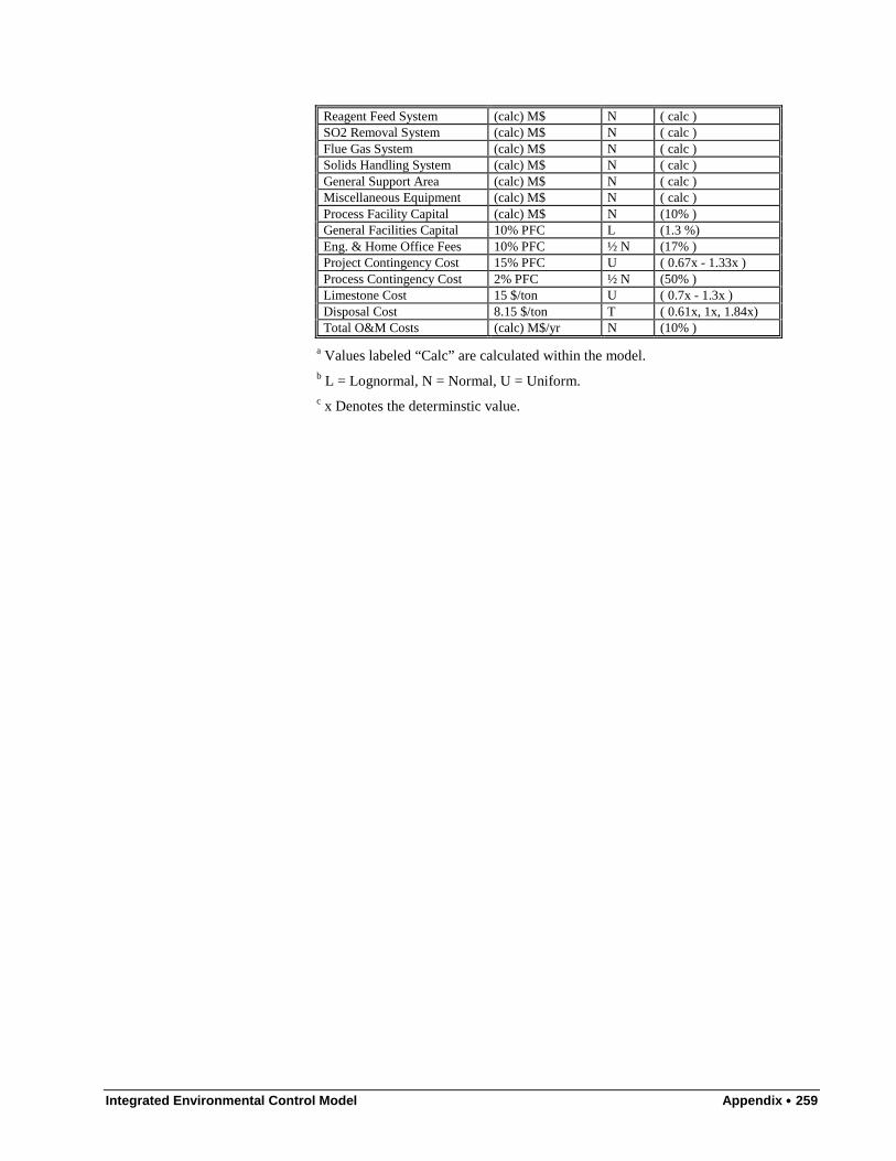
Integrated Environmental Control Model Appendix •••• 259
Reagent Feed System (calc) M$ N ( calc )SO2 Removal System (calc) M$ N ( calc )Flue Gas System (calc) M$ N ( calc )Solids Handling System (calc) M$ N ( calc )General Support Area (calc) M$ N ( calc )Miscellaneous Equipment (calc) M$ N ( calc )Process Facility Capital (calc) M$ N (10% )General Facilities Capital 10% PFC L (1.3 %)Eng. & Home Office Fees 10% PFC ½ N (17% )Project Contingency Cost 15% PFC U ( 0.67x - 1.33x )Process Contingency Cost 2% PFC ½ N (50% )Limestone Cost 15 $/ton U ( 0.7x - 1.3x )Disposal Cost 8.15 $/ton T ( 0.61x, 1x, 1.84x)Total O&M Costs (calc) M$/yr N (10% )
a Values labeled “Calc” are calculated within the model.b L = Lognormal, N = Normal, U = Uniform.c x Denotes the determinstic value.
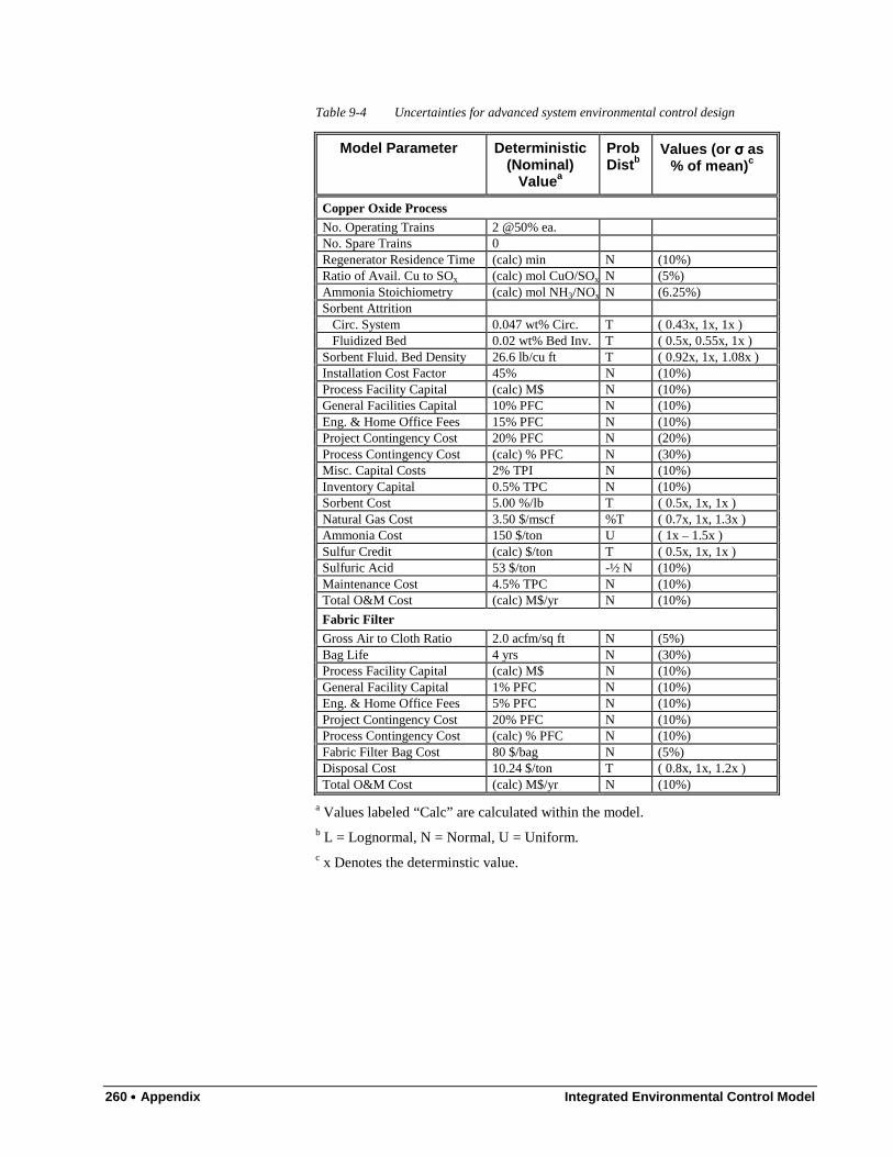
260 •••• Appendix Integrated Environmental Control Model
Table 9-4 Uncertainties for advanced system environmental control design
Model Parameter Deterministic(Nominal)
Valuea
ProbDist b
Values (or σσσσ as% of mean) c
Copper Oxide Process
No. Operating Trains 2 @50% ea.No. Spare Trains 0Regenerator Residence Time (calc) min N (10%)Ratio of Avail. Cu to SOx (calc) mol CuO/SOx N (5%)Ammonia Stoichiometry (calc) mol NH3/NOx N (6.25%)Sorbent Attrition Circ. System 0.047 wt% Circ. T ( 0.43x, 1x, 1x ) Fluidized Bed 0.02 wt% Bed Inv. T ( 0.5x, 0.55x, 1x )Sorbent Fluid. Bed Density 26.6 lb/cu ft T ( 0.92x, 1x, 1.08x )Installation Cost Factor 45% N (10%)Process Facility Capital (calc) M$ N (10%)General Facilities Capital 10% PFC N (10%)Eng. & Home Office Fees 15% PFC N (10%)Project Contingency Cost 20% PFC N (20%)Process Contingency Cost (calc) % PFC N (30%)Misc. Capital Costs 2% TPI N (10%)Inventory Capital 0.5% TPC N (10%)Sorbent Cost 5.00 %/lb T ( 0.5x, 1x, 1x )Natural Gas Cost 3.50 $/mscf %T ( 0.7x, 1x, 1.3x )Ammonia Cost 150 $/ton U ( 1x – 1.5x )Sulfur Credit (calc) $/ton T ( 0.5x, 1x, 1x )Sulfuric Acid 53 $/ton -½ N (10%)Maintenance Cost 4.5% TPC N (10%)Total O&M Cost (calc) M$/yr N (10%)
Fabric FilterGross Air to Cloth Ratio 2.0 acfm/sq ft N (5%)Bag Life 4 yrs N (30%)Process Facility Capital (calc) M$ N (10%)General Facility Capital 1% PFC N (10%)Eng. & Home Office Fees 5% PFC N (10%)Project Contingency Cost 20% PFC N (10%)Process Contingency Cost (calc) % PFC N (10%)Fabric Filter Bag Cost 80 $/bag N (5%)Disposal Cost 10.24 $/ton T ( 0.8x, 1x, 1.2x )Total O&M Cost (calc) M$/yr N (10%)
a Values labeled “Calc” are calculated within the model.b L = Lognormal, N = Normal, U = Uniform.c x Denotes the determinstic value.
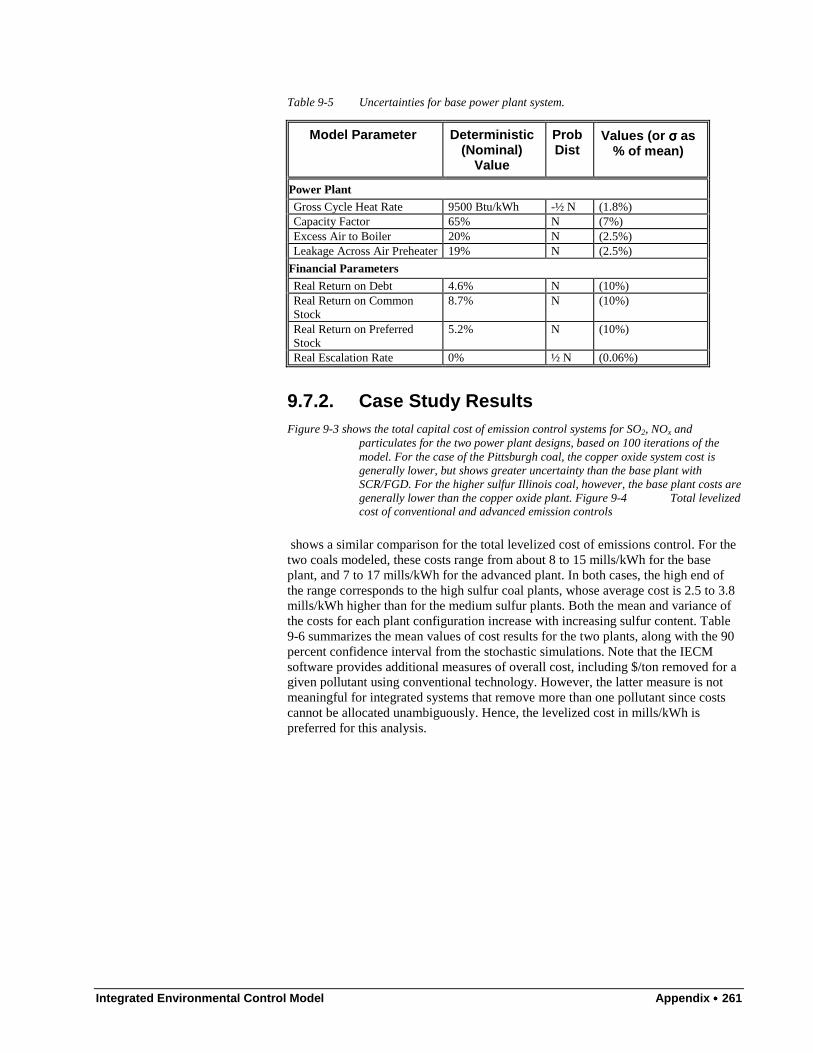
Integrated Environmental Control Model Appendix •••• 261
Table 9-5 Uncertainties for base power plant system.
Model Parameter Deterministic(Nominal)
Value
ProbDist
Values (or σσσσ as% of mean)
Power Plant
Gross Cycle Heat Rate 9500 Btu/kWh -½ N (1.8%)Capacity Factor 65% N (7%)Excess Air to Boiler 20% N (2.5%)Leakage Across Air Preheater 19% N (2.5%)
Financial Parameters
Real Return on Debt 4.6% N (10%)Real Return on CommonStock
8.7% N (10%)
Real Return on PreferredStock
5.2% N (10%)
Real Escalation Rate 0% ½ N (0.06%)
9.7.2. Case Study ResultsFigure 9-3 shows the total capital cost of emission control systems for SO2, NOx and
particulates for the two power plant designs, based on 100 iterations of themodel. For the case of the Pittsburgh coal, the copper oxide system cost isgenerally lower, but shows greater uncertainty than the base plant withSCR/FGD. For the higher sulfur Illinois coal, however, the base plant costs aregenerally lower than the copper oxide plant. Figure 9-4 Total levelizedcost of conventional and advanced emission controls
shows a similar comparison for the total levelized cost of emissions control. For thetwo coals modeled, these costs range from about 8 to 15 mills/kWh for the baseplant, and 7 to 17 mills/kWh for the advanced plant. In both cases, the high end ofthe range corresponds to the high sulfur coal plants, whose average cost is 2.5 to 3.8mills/kWh higher than for the medium sulfur plants. Both the mean and variance ofthe costs for each plant configuration increase with increasing sulfur content. Table9-6 summarizes the mean values of cost results for the two plants, along with the 90percent confidence interval from the stochastic simulations. Note that the IECMsoftware provides additional measures of overall cost, including $/ton removed for agiven pollutant using conventional technology. However, the latter measure is notmeaningful for integrated systems that remove more than one pollutant since costscannot be allocated unambiguously. Hence, the levelized cost in mills/kWh ispreferred for this analysis.
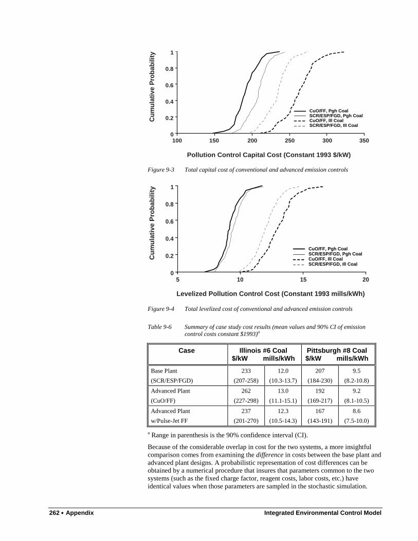
262 •••• Appendix Integrated Environmental Control Model
Cum
ulat
ive
Pro
babi
lity
Pollution Control Capital Cost (Constant 1993 $/kW)
100 150 200 250 300 3500
0.2
0.4
0.6
0.8
1
CuO/FF, Pgh CoalSCR/ESP/FGD, Pgh CoalCuO/FF, Ill CoalSCR/ESP/FGD, Ill Coal
Figure 9-3 Total capital cost of conventional and advanced emission controls
CuO/FF, Pgh CoalSCR/ESP/FGD, Pgh CoalCuO/FF, Ill CoalSCR/ESP/FGD, Ill Coal
Cu
mu
lati
ve P
rob
abili
ty
Levelized Pollution Control Cost (Constant 1993 mills/kWh)
5 10 15 200
0.2
0.4
0.6
0.8
1
Figure 9-4 Total levelized cost of conventional and advanced emission controls
Table 9-6 Summary of case study cost results (mean values and 90% CI of emissioncontrol costs constant $1993)a
Case Illinois #6 Coal$/kW mills/kWh
Pittsburgh #8 Coal$/kW mills/kWh
Base Plant
(SCR/ESP/FGD)
233
(207-258)
12.0
(10.3-13.7)
207
(184-230)
9.5
(8.2-10.8)
Advanced Plant
(CuO/FF)
262
(227-298)
13.0
(11.1-15.1)
192
(169-217)
9.2
(8.1-10.5)
Advanced Plant
w/Pulse-Jet FF
237
(201-270)
12.3
(10.5-14.3)
167
(143-191)
8.6
(7.5-10.0)
a Range in parenthesis is the 90% confidence interval (CI).
Because of the considerable overlap in cost for the two systems, a more insightfulcomparison comes from examining the difference in costs between the base plant andadvanced plant designs. A probabilistic representation of cost differences can beobtained by a numerical procedure that insures that parameters common to the twosystems (such as the fixed charge factor, reagent costs, labor costs, etc.) haveidentical values when those parameters are sampled in the stochastic simulation.
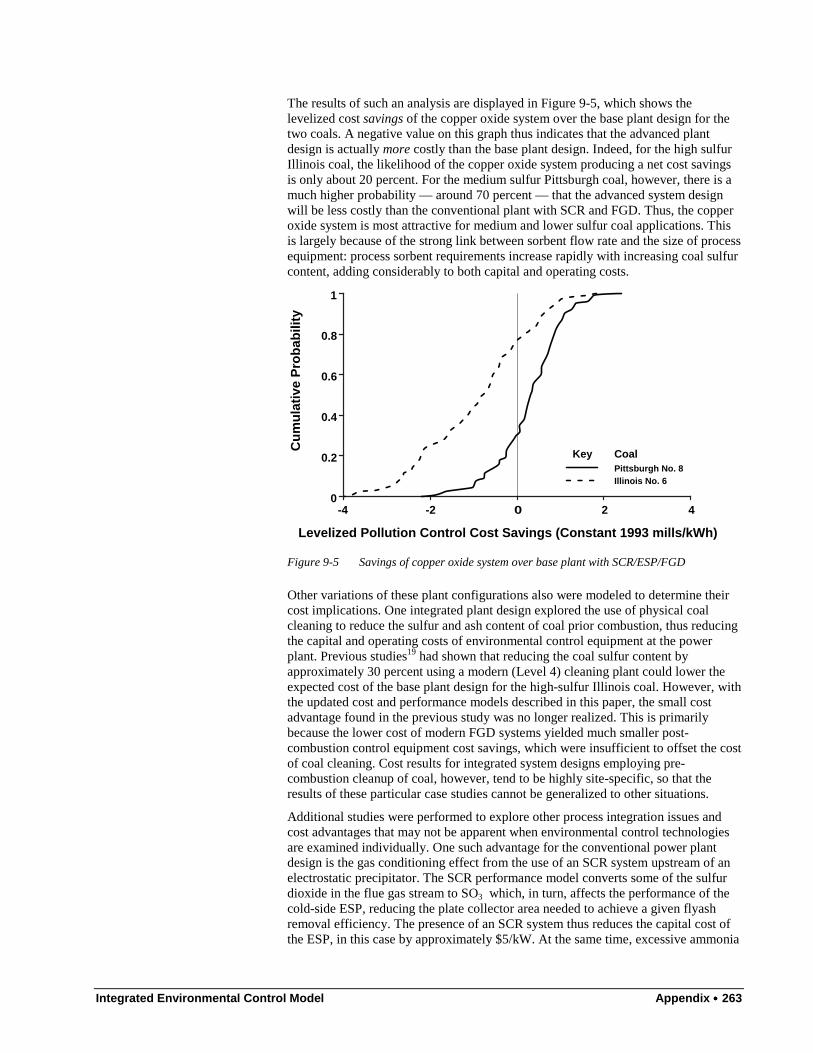
Integrated Environmental Control Model Appendix •••• 263
The results of such an analysis are displayed in Figure 9-5, which shows thelevelized cost savings of the copper oxide system over the base plant design for thetwo coals. A negative value on this graph thus indicates that the advanced plantdesign is actually more costly than the base plant design. Indeed, for the high sulfurIllinois coal, the likelihood of the copper oxide system producing a net cost savingsis only about 20 percent. For the medium sulfur Pittsburgh coal, however, there is amuch higher probability — around 70 percent — that the advanced system designwill be less costly than the conventional plant with SCR and FGD. Thus, the copperoxide system is most attractive for medium and lower sulfur coal applications. Thisis largely because of the strong link between sorbent flow rate and the size of processequipment: process sorbent requirements increase rapidly with increasing coal sulfurcontent, adding considerably to both capital and operating costs.
Cu
mu
lati
ve P
rob
abili
ty
Levelized Pollution Control Cost Savings (Constant 1993 mills/kWh)
-4 -2 20 40
0.2
0.4
0.6
0.8
1
Key CoalPittsburgh No. 8Illinois No. 6
Figure 9-5 Savings of copper oxide system over base plant with SCR/ESP/FGD
Other variations of these plant configurations also were modeled to determine theircost implications. One integrated plant design explored the use of physical coalcleaning to reduce the sulfur and ash content of coal prior combustion, thus reducingthe capital and operating costs of environmental control equipment at the powerplant. Previous studies19 had shown that reducing the coal sulfur content byapproximately 30 percent using a modern (Level 4) cleaning plant could lower theexpected cost of the base plant design for the high-sulfur Illinois coal. However, withthe updated cost and performance models described in this paper, the small costadvantage found in the previous study was no longer realized. This is primarilybecause the lower cost of modern FGD systems yielded much smaller post-combustion control equipment cost savings, which were insufficient to offset the costof coal cleaning. Cost results for integrated system designs employing pre-combustion cleanup of coal, however, tend to be highly site-specific, so that theresults of these particular case studies cannot be generalized to other situations.
Additional studies were performed to explore other process integration issues andcost advantages that may not be apparent when environmental control technologiesare examined individually. One such advantage for the conventional power plantdesign is the gas conditioning effect from the use of an SCR system upstream of anelectrostatic precipitator. The SCR performance model converts some of the sulfurdioxide in the flue gas stream to SO3 which, in turn, affects the performance of thecold-side ESP, reducing the plate collector area needed to achieve a given flyashremoval efficiency. The presence of an SCR system thus reduces the capital cost ofthe ESP, in this case by approximately $5/kW. At the same time, excessive ammonia

264 •••• Appendix Integrated Environmental Control Model
slip in an SCR system can affect the salability of collected flyash for byproductapplications. In the present case studies all flyash is assumed to be disposed in alandfill, and ammonia slip is kept to a nominal design level of 5 ppmv. However, theeffect of alternative ammonia slip levels on overall plant economics, includingbyproduct credits for flyash, is readily modeled in the IECM.
For the copper oxide system, a key integration issue involves tradeoffs regarding theair preheater and downstream particulate collector. In order to fully recover theenergy released in exothermic chemical reactions associated with sulfur removal, alarger (more expensive) air preheater is required. If the preheater is not re-sized, thehigher flue gas temperature generated by the copper oxide system increases thecapital cost of downstream particulate equipment, whose cost depends on the actualvolumetric gas flow rate. Thus, an integrated analysis is required to determine theleast-cost solution for a particular application.
Another integration issue for the advanced plant design is the choice of particulatecollector downstream of the SO2/NOx removal system. In the examples above, aconventional reverse gas fabric filter was assumed. In this application, a fabric filteris preferable to an ESP because of the low sulfur content of the flue gas. However,advanced fabric filter technology employing a pulse jet system instead of currentreverse gas cleaning offers the potential to reduce the capital cost of the advancedplant design by at least $25/kW, according to the results of additional analysis. On alevelized cost basis, this improves the likelihood of the copper oxide plant designbeing less costly than the conventional system. For example, for the plant burningPittsburgh seam coal the probability of a cost savings increases to approximately 90percent with a pulse jet fabric filter, as compared to 70 percent with the conventionalreverse gas system (Figure 9-6). The absolute value of expected cost savings alsoincreases as the cumulative probability distributions in Figure 9-5 shift toward theright.
Cu
mu
lati
ve P
rob
abili
ty
Levelized Pollution Control Cost Savings (Constant 1993 mills/kWh)
-4 -2 0 2 40
0.2
0.4
0.6
0.8
1
Key Fabric Filter TypePulse JetReverse Gas
Pittsburgh No. 8 Coal
Figure 9-6 Effect of fabric filter choice on cost savings for copper oxide system
9.8. DiscussionThe results presented here can be a starting point for further analyses to explore theprimary sources of uncertainty, and the potential for R&D to improve performanceand lower costs by reducing the uncertainties that matter most. Other recentpapers12,20 illustrate how results from the IECM can be used in conjunction with
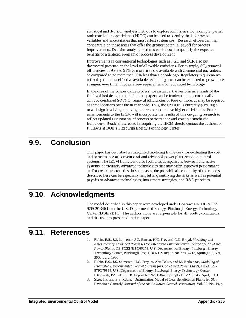
Integrated Environmental Control Model Appendix •••• 265
statistical and decision analysis methods to explore such issues. For example, partialrank correlation coefficients (PRCC) can be used to identify the key processvariables and uncertainties that most affect system cost. Research efforts can thenconcentrate on those areas that offer the greatest potential payoff for processimprovements. Decision analysis methods can be used to quantify the expectedbenefits of a targeted program of process development.
Improvements in conventional technologies such as FGD and SCR also putdownward pressure on the level of allowable emissions. For example, SO2 removalefficiencies of 95% to 98% or more are now available with commercial guarantees,as compared to no more than 90% less than a decade ago. Regulatory requirementsreflecting the most effective available technology thus can be expected to grow morestringent over time, imposing new requirements for advanced technology.
In the case of the copper oxide process, for instance, the performance limits of thefluidized bed design modeled in this paper may be inadequate to economicallyachieve combined SO2/NOx removal efficiencies of 95% or more, as may be requiredat some locations over the next decade. Thus, the USDOE is currently pursuing anew design involving a moving bed reactor to achieve higher efficiencies. Futureenhancements to the IECM will incorporate the results of this on-going research toreflect updated assessments of process performance and cost in a stochasticframework. Readers interested in acquiring the IECM should contact the authors, orP. Rawls at DOE’s Pittsburgh Energy Technology Center.
9.9. ConclusionThis paper has described an integrated modeling framework for evaluating the costand performance of conventional and advanced power plant emission controlsystems. The IECM framework also facilitates comparisons between alternativesystems, particularly advanced technologies that may offer improved performanceand/or cost characteristics. In such cases, the probabilistic capability of the modelsdescribed here can be especially helpful in quantifying the risks as well as potentialpayoffs of advanced technologies, investment strategies, and R&D priorities.
9.10. AcknowledgmentsThe model described in this paper were developed under Contract No. DE-AC22-92PC91346 from the U.S. Department of Energy, Pittsburgh Energy TechnologyCenter (DOE/PETC). The authors alone are responsible for all results, conclusionsand discussions presented in this paper.
9.11. References1. Rubin, E.S., J.S. Salmento, J.G. Barrett, H.C. Frey and C.N. Bloyd, Modeling and
Assessment of Advanced Processes for Integrated Environmental Control of Coal-FiredPower Plants, DE-FG22-83PC60271, U.S. Department of Energy, Pittsburgh EnergyTechnology Center, Pittsburgh, PA; also NTIS Report No. 86014713, Springfield, VA,396p, July, 1986.
2. Rubin, E.S., J.S. Salmento, H.C. Frey, A. Abu-Baker, and M. Berkenpas, Modeling ofIntegrated Environmental Control Systems for Coal-Fired Power Plants, DE-AC22-87PC79864, U.S. Department of Energy, Pittsburgh Energy Technology Center,Pittsburgh, PA; also NTIS Report No. 92016847, Springfield, VA, 214p, April, 1991.
3. Skea, J.F. and E.S. Rubin, “Optimization Model of Coal Benefication Plants for SO2
Emissions Control,” Journal of the Air Pollution Control Association, Vol. 38, No. 10, p.
266 •••• Appendix Integrated Environmental Control Model
1281-1288, October, 1988.4. Technical Assessment Guide, Electric Supply — 1993, EPRI TR-102276, Electric Power
Research Institute, Palo Alto, CA, 1993. Also, private communication with Dr. C.McGowin, EPRI, 1995.
5. Kalagnanam, J.R., and E.S. Rubin, Cost Models for Pulverized Coal Base Plants, DE-AC22-92PC91346-10, U.S. Department of Energy, Pittsburgh Energy TechnologyCenter, Pittsburgh, PA; also NTIS Report No. 95015602, Springfield, VA, April, 1995.
6. Frey, H.C., "Engineering-Economic Evaluation of SCR NOx Control Systems for Coal-Fired Power Plants", Proceedings of the American Power Conference, Vol. 57, IllinoisInstitute of Technology, Chicago, Illinois. April 1995.
7. Lowe, P.A., W. Ellison, and M. Perlsweig, “Understanding the German and JapaneseCoal-Fired SCR Experience,” Proceedings of 1991 Symposium on StationaryCombustion Nitrogen Oxide Control, Electric Power Research Institute, Palo Alto, CA,March 1991.
8. Kalagnanam, J.R. and E.S. Rubin, Performance and Cost Models for ElectrostaticPrecipitators, DE-AC22-92PC91346-7, U.S. Department of Energy, Pittsburgh EnergyTechnology Center, Pittsburgh, PA; also NTIS Report No. 95001968, Springfield, VA,July, 1994.
9. Kalagnanam, J.R. and E.S. Rubin, Performance and Cost Models for Fabric Filters, DE-AC22-92PC91346-6, U.S. Department of Energy, Pittsburgh Energy Technology Center,Pittsburgh, PA; also NTIS Report No. 94014551, Springfield, VA, April, 1994.
10. Gaikwad, R.P. and D.G. Sloat, Economic Evaluation of Particulate ControlTechnologies, Report No. EPRI TR-100748, Electric Power Research Institute, Palo Alto,CA, 1992.
11. Sloat, D.G., R.P. Gaikwad and R.L. Chang, “The Potential of Pulse-Jet Baghouses forUtility Boilers. Part 3: Comparative Economics of Pulse-Jet Baghouse, Precipitators andReverse-Gas Baghouses,” J. Air & Waste Management Assoc., 43, 120, 1993.
12. Rubin, E. S., J.R. Kalagnanam and M.B. Berkenpas, “New Models for FGDPerformance, Cost and Hazardous Air Pollutant Removal,” Proceedings of 1995 SO2
Control Symposium, Electric Power Research Institute, Palo Alto, CA, March, 1995.13. Keeth, R.J., D.L. Baker, P.E. Tracy, G.E. Ogden and P.A. Ireland, Economic Evaluation
of Flue Gas Desulfurization Systems, GS-7193, RP1610-6, Electric Power ResearchInstitute, Palo Alto, CA 1991.
14. Kalagnanam, J.R. and E.S. Rubin, Performance and Cost Models for Flue GasDesulfurization Processes, DE-AC22-92PC91346-11, U.S. Department of Energy,Pittsburgh Energy Technology Center, Pittsburgh, PA; also NTIS Report No. 9600352,Springfield, VA, June, 1995.
15. Frey, H.C., "Performance Model of the Fluidized Bed Copper Oxide Process forSO2/NOx Control," Paper No. 93-WA-79.01, Proceedings of the 86th Annual Meeting,Air and Waste Management Association, Pittsburgh, PA, June 1993.
16. Kalagnanam, J.R. and E.S. Rubin, Performance and Cost Models for the NOXSOProcess, DE-AC22-92PC91346-12, U.S. Department of Energy, Pittsburgh EnergyTechnology Center, Pittsburgh, PA; also NTIS Report No. 96009831, Springfield, VA,December, 1995.
17. Lumina Decision Systems, Analytica User Guide: Release 1.0, Lumina DecisionSystems, Los Altos, CA, 1996.
18. Berkenpas, M.B. and E.S. Rubin, IECM User’s Manual, Prepared for U.S. Department ofEnergy, Pittsburgh Energy Technology Center, by Center for Energy and EnvironmentalStudies, Carnegie Mellon University, Pittsburgh, PA, 1996.
19. Frey, H.C. and E.S. Rubin, "Probabilistic Evaluation of Advanced SO2/NOx ControlTechnology," Journal of Air & Waste Management Association, Vol. 41, No. 12, p.1585-1593, December, 1991.
20. Frey, H.C. and E.S. Rubin, "Evaluation Method for Advanced Acid Rain ComplianceTechnology," Journal of Energy Engineering, Vol. 118, No. 1, p. 38-55, April, 1992.

Integrated Environmental Control Model Glossary of Terms •••• 267
10. Glossary of Terms


Integrated Environmental Control Model Index •••• 269
11. Index
Error! No index entries found.