technical documentation to support development of minimum
TRANSCRIPT

Technical Documentation to Support Developmentof Minimum Flows and Levels for the
Caloosahatchee River and Estuary
Appendices
Contents
Title Page No.
Appendix A - Caloosahatchee River MFL Research ProgramProgress Report A-1
Appendix B - Effects of seasonal and water quality parameters onoysters (Crassostrea virginica) and associated fishpopulations in the Caloosahatchee River. B-1
Appendix C -- Impacts of Freshwater Inflows on the Distribution ofZooplankton and Ichthyoplankton in the CaloosahatcheeEstuary, Florida C-1
Appendix D -- Salinity Tolerance of Vallisneria and Salinity Criteria D-1
Appendix E -- CERP Projects in the C-43 Basin E-1
Appendix F -- Hydrodynamic and Salinity Modeling F-1
Appendix G -- The Significance of Tidal Runoff on Flows to theCaloosahatchee Estuary G-1
Appendix H -- Development of an ecological model to predict Vallisneriaamericana Michx. densities in the upper CaloosahatcheeEstuary: MFL update H-1

Technical Documentation to Support Development ofMinimum Flows and Levels for the Caloosahatchee
River and Estuary
Appendix A
Caloosahatchee River MFL Research ProgramProgress Report
Contents
Introduction ............................................................................................................................A-1Research Program Components...............................................................................................A-1
Component 1. CH3D Hydrodynamic salinity model of Calooshatchee: ..............................A-1Component 2. Population model for Vallisneria americana................................................A-2Component 3. Additional Experimental Studies .................................................................A-3Component 4. Quantify the habitat value of Vallisneria americana beds ............................A-3Component 5. Effects of MFL flows on other biota, especially those located downstream..A-3
Flow Effects on Oysters ..................................................................................................A-3Effects of Flows on Zooplankton and Ichthyoplankton: ...................................................A-4
Component 6. Monitoring of Vallisneria americana beds...................................................A-4Component 7. Vallisneria americana Restoration and Seed Bank Studies ..........................A-4
Literature Cited.......................................................................................................................A-4
Florida Bay and Lower West Coast DivisionSouthern District Restoration Department
South Florida Water Management District
January 2003


Caloosahatchee MFL 2002 Status Update Report Appendix A -- Research Program
02/03/03 10:32 AM A-1 DRAFT
Caloosahatchee River MFL Research Program -- Progress Report
Introduction
As part of the development of the Caloosahatchee MFL, a scientific peer review of the technical
criteria was conducted and a report produced (Edwards et al 2000). Comments from the public
and other State and Federal agencies also were solicited. The review committee approved the
general scientific approach used in establishing the MFL. However, specific scientific
deficiencies in the technical documentation of the rule were identified. A research program was
initiated to address these concerns and included additional field observations, laboratory
experiments and development of modeling tools. Major criticisms of the initial effort were:
1. Lack of a hydrodynamic/salinity model
2. Lack of a population model for Vallisneria americana
3. No quantification of the habitat value of V. americana beds
4. Effects of MFL flows on downstream estuarine biota
Research Program Components:
Component 1: CH3D Hydrodynamic salinity model of Caloosahatchee:
Background: A CH3D hydrodynamic model originally developed for the entire Charlotte
Harbor system is being adapted for use in the Caloosahatchee. The model is three dimensional,
time-dependant and employs a curvilinear grid. The purpose of the modeling effort is two-fold.
The first is to simulate the distribution of salinity in the estuary under minimum flow conditions.
The present MFL rule states that a discharge of 300 cfs at S-79 is necessary to maintain a salinity
of 10 ppt at the Ft. Myers Yacht Basin. The model will be used to evaluate this proposition.
The second use of the model will be to reconstruct the 31-year salinity history in the protected
area under different land use conditions in the watershed. Specifically, conditions with and
without CERP projects will be contrasted. The CERP Projects are the recovery strategy for the
MFL and this exercise will evaluate this strategy.

Caloosahatchee MFL 2002 Status Update Report Appendix A -- Research Program
02/03/03 10:32 AM A-2 DRAFT
Status: The model has been calibrated using a 3-month data set, without ground water input.
Validation using an additional 3 months is underway. Flow vs salinity distribution curves for
constant discharges have been developed. A multiple regression model that relates daily salinity
at Ft. Myers and at Bridge 31 to discharge at S-79 has been developed and calibrated using a10
year period of daily salinity data. It is now possible to predict daily average salinity for 31 years
at Ft. Myers, Rte. 31 Bridge and through interpolation, two stations located between Ft. Myers
and Bridge 31.
Future Improvements: The District is working to improve the CH3D model. The model has
inadequate bathymetry and a survey of the Caloosahatchee is planned for FY03. Further
calibration and validation are required with groundwater and tributary input from the tidal basin.
The speed of the model will be improved by acquisition of a new parallel code and grid editor.
Component 2: Population model for Vallisneria americana
Background: A Stella based population level model of V. americana in the Caloosahatchee is
currently under development. The purpose is to include more environmental factors than just
salinity and arrive at a better estimate of the effects of freshwater inflow on performance of V.
americana. In conjunction with 31 years of salinity data, the model will be used to evaluate
present and future ability to meet MFL. The model will not be totally complete in time for the
criteria review. Nevertheless, we will attempt to use the model as it is.
Status: The original model had one forcing function: salinity. The new model has salinity, light,
and temperature. The model has been calibrated using four years of data (1998-2001). At
present, the model can simulate growth of V. americana at two stations in the protected area of
the estuary.
Future Improvements: Additional input data and information concerning the growth and
survival of V. americana in the Caloosahatchee Estuary will be required to make the model more
robust. Specific needs are to:
1. Develop a method to predict variation in water transparency for long-term or other
simulations.

Caloosahatchee MFL 2002 Status Update Report Appendix A -- Research Program
02/03/03 10:32 AM A-3 DRAFT
2. Develop relationships to relate mass to blade and shoot densities, and blade length with
existing data.
3. Develop improved algorithms for light and salinity.
4. Incorporate blade length as a state variable to more accurately represent light availability
for mature plants.
5. Add population and demographic characteristics to describe seed production and
dispersal.
Component 3: Additional Experimental Studies
Background: Two experiments at the Gumbo Limbo Mesocosm Facility will provide addition
data for the V. americana modeling effort. An experiment quantifying the response of V.
americana to high salinity has already been conducted. We now have data on growth and
mortality of V. americana at salinities ranging from 0 to 30 ppt. An experiment evaluating the
interaction of light and salinity was conducted in April and May, 2002.
Status: Both experiments have been conducted. Results of the first have been incorporated into
the model. Results of the second will not be available for this review.
Component 4: Quantify the habitat value of Vallisneria americana beds
Background: This is being accomplished through a contract (C-12836) with Mote Marine Lab
(3 years). The overall objective is to identify which organisms use V. americana habitat in the
Caloosahatchee River and how season, salinity and plant /bed morphometry affect habitat use.
Status: The study began in January of 2002. Results will not be available for this review.
Component 5: Effects of MFL flows on other biota, especially those located downstream
Flow Effects on Oysters
Background: Effects of low flows on downstream oysters, Crassostrea virginica, are being
examined through a contract (C-12412) with Florida Gulf Coast University. The objectives of
this study are several fold:
1. To examine seasonally the mortality and disease prevalence.
2. To investigate growth, mortality and reproductive potential of oysters under various
salinity regimes.

Caloosahatchee MFL 2002 Status Update Report Appendix A -- Research Program
02/03/03 10:32 AM A-4 DRAFT
3. To study oyster spat settlement as a function of salinity.
4. To investigate the role of oyster reefs as essential fish habitat and determine whether
the condition of individual oysters affects overall habitat suitability.
Status: Dr. Volety, Principal Investigator, has submitted a progress report (July 2002) that
addresses the freshwater inflow requirements of oysters in the Caloosahatchee.
Effects of Flows on Zooplankton and Ichthyoplankton
Background: The District has monitored zooplankton and larval planktonic fish at 7 stations in
the Caloosahatchee Estuary, San Carlos Bay under a range of freshwater discharge conditions at
S-79. Monitoring was not continuous but occurred on a monthly basis during the following
periods 1986 – 1989, 1994-1995, and 1998. Data have been analyzed to investigate the effects
of discharge on the abundance and distribution of these groups in the estuary.
Component 6: Monitoring of Vallisneria americana beds.
Background: A monthly monitoring program at four stations was initiated in 1998. The data are
used to examine potential effects of salinity and other water quality parameters on Vallisneria.
Status: On-going
Component 7. Vallisneria americana Restoration and Seed Bank Studies
Background: These studies are being carried out through contract with the Conservancy of
Southwest Florida and are intended to:
1. Determine the importance of the seed bank in reestablishing tape grass
2. Determine if planting seagrasses enhances their reestablishment
3. Establish the optimal conditions and methods for tape grass re-vegetation
4. Calculate an effort (time, expenditure) budget for a tape grass restoration program
Status: Started August 2003. On-going
Literature Cited
Edwards, R. E., W. Lung, P.A. Montagna, and H. L. Windom. 2000. Final review report.Caloosahatchee Minimum Flow Peer Review Panel, September 27-29, 2000. Report tothe South Florida Water Management District, West Palm Beach, FL.

Technical Documentation to Support Development ofMinimum Flows and Levels for the Caloosahatchee
River and Estuary
Appendix B
Effects of seasonal and water quality parameters onoysters (Crassostrea virginica) and associated fish
populations in the Caloosahatchee River.
Contents
Abstract ....................................................................................................................................... B-2Introduction................................................................................................................................. B-3Materials and Methods................................................................................................................ B-4Results......................................................................................................................................... B-5Summary and Conclusions ......................................................................................................... B-6References................................................................................................................................... B-8
Progress Report submittedto
Dr. Peter Doering
July 2002.
Aswani K. Volety and S. Greg Tolley.Florida Gulf Coast University
10501 FGCU Boulevard SouthFort Myers, FL 33912.


Effects of seasonal and water quality parameters on oysters (Crassostrea virginica)
and associated fish populations in the Caloosahatchee River.
Progress Report submitted
to
Dr. Peter Doering
July 2002.
Aswani K. Volety and S. Greg Tolley.
Florida Gulf Coast University 10501 FGCU Boulevard South
Fort Myers, FL 33912.

Abstract Disease prevalence (% infected oysters) and intensity of oyster pathogen, Perkinsus marinus, were investigated at five locations (Piney Point, Cattle Dock, Bird Island, Kitchel Key and Tarpon Bay) in the Caloosahatchee Estuary in relation to season and freshwater releases (i.e., salinity) from Lake Okeechobee. Ten oysters per month were analyzed from each sampling location during September 2000 - June 2002. Data were analyzed as year 1 (September 2000 - August 2001) and Year 2 (September 2001 - June 2002). Freshwater releases > 300 cubic feet per second (CFS) from Lake Okeechobee by the South Florida Water Management District (SFWMD) during dry months (Nov - May) in year 2 resulted in lower salinities at all locations compared to year 1. Freshwater releases during the dry months in Year 1 were less than 300 CFS. Salinities during sample collection were regressed against monthly average of 30-day moving average flow to predict salinity changes at the sampling locations. Results suggest that freshwater releases of 1000 CFS from Lake Okeechobee may decrease salinities at the sampling locations by 3.6 - 6 ppt (downstream - upstream locations) from respective prevailing salinities. Salinity, and temperature during the study period ranged from 3 - 40 ppt and from 16 - 32ºC respectively. Prevalence of P. marinus ranged from 0 - 90% while the intensity of infection ranged from 0 - 2.5 (on a scale of 0 - 5). Concomitant with higher freshwater releases and lower salinities at all sampling locations in year 2, intensity of P. marinus infection in oysters was significantly lower during year 2 compared to year 1. Infection intensity was also significantly different between sampling locations. It should be noted that while the prevalence of infection was high, overall infection intensities at various sampling locations were light (0.170 - 0.753) during both years suggesting that decreased freshwater releases less than 300 CFS (and higher salinities) did not result in lethal (heavy) infection intensities. Flows between 500 and 2000 CFS will result in optimum salinities for oysters and will result in sustaining and enhancing oyster populations in the Caloosahatchee Estuary. Data suggests that well-timed fresh water releases into Caloosahatchee River may prevent or lower P. marinus infections to non-lethal levels (light) in oysters and enable them to survive longer. Effects of high freshwater releases (and lowered salinities) on the condition index, recruitment, gonadal index, and growth of juvenile oysters are being examined in a series of field and laboratory experiments. The use of adaptive management approaches involving freshwater releases to sustain and enhance oyster populations is valuable to the ecology of the Caloosahatchee Estuary.
Introduction A fundamental management goal of the Watershed Research and Planning Department is to “Protect, Enhance, and Rehabilitate Estuarine Ecosystems”. Using a suite of responses from Valued Ecosystem Component (VEC) species - oysters - the effects of freshwater releases from Lake Okeechobee were assessed. VEC species are those that sustain the ecological structure and function of dominant estuarine communities. These species provide not only food, but also the physical habitat utilized by other organisms for living space, refuge, and foraging sites. Examples of dominant estuarine communities are oyster bars and grass beds, with prominent species being the American oyster, Crassostrea virginica and the submerged aquatic vegetation (SAVs), Vallisneria americana, Halodule wrightii, and Thalassia testudinum. Historically, grass beds and osyter reefs have been dominant components of the Caloosahatchee estuarine system. Both habitat types still exist in the system today.
Oysters not only represent an important fisheries species commonly found in
estuaries of the Atlantic and Gulf coasts of the U.S., but they are important ecologically. Individual oysters filter 4-34 liters of water per hour, removing phytoplankton, particulate organic carbon, sediments, pollutants, and microorganisms from the water column. This filtration process results in greater light penetration immediately downstream, thus promoting the growth of submerged aquatic vegetation. Although oysters assimilate 70% of the organic matter filtered, the remainder is deposited on the bottom where it provides food for benthic organisms. This secondary production, combined with a complex, three-dimensional, reef structure serving as nesting habitat and/or refuge, attracts numerous species of invertebrates and fishes (e.g., blue crab, mud crabs, grass shrimps, penaeid shrimp, blennies, gobies, killifishes, skilletfish, toadfishes). Furthermore, many of these organisms serve as forage for important fisheries species, birds, and mammals. Oysters are not only an important fisheries species, but oyster reefs serve as essential fish habitat. Due to their sessile nature, oysters make excellent candidates to investigate cause and effects relationship in examining watershed alteration effects. Due to the ecological role of oysters, their protection and restoration should therefore be a focus of resource managers.
The protozoan parasite, Perkinsus marinus has devastated oyster populations in
the Atlantic (Burreson and Ragone-Calvo 1996), where it is currently the primary pathogen of oysters, and in the Gulf of Mexico (Soniat 1996). Andrews (1988) estimated that P. marinus can kill ~80% of the oysters in a bed. The distribution and prevalence of P. marinus is influenced by temperature and salinity with higher values favoring the disease organism (Burreson and Ragone-Calvo 1996, Soniat 1996, Chu and Volety 1997).
While the South Florida Water Management District (SFWMD) has conducted
considerable research on SAV (Chamberlain and Doering 1998a, Chamberlain and Doering 1998b, Kraemer et al. 1999), studies involving other valued ecosystem components, such as oyster reefs, that occur in the higher salinity waters of the lower Caloosahatchee Estuary are presently lacking, but clearly necessary. To our knowledge,

this project represents the first study of oysters in the Caloosahatchee River and will provide critical information for use in applying the VEC approach. The ultimate goal of this project is examine the effect of minimum flows and levels of freshwater into the Caloosahatchee Estuary and to provide target conditions for watershed management in the Caloosahatchee River that will sustain and enhance oyster populations.
This report summarizes the results of Perkinsus marinus infection prevalence and intensities in oysters from Caloosahatchee River during September 2000 - June 2002, focusing on the dry months (November - May). The overall objectives of the project were to evaluate the effect of season and spatial variation on condition and health of oyster populations in the Caloosahatchee and to determine the suitability of oyster habitat to crustaceans and fishes in relation to oyster health and condition. Results related to spat recruitment potential, and habitat suitability of oyster reefs for crustaceans and fishes in the Caloosahatchee River will be addressed in the next report. Materials and Methods Sampling Locations: Monthly water quality measurements and oyster collections were made at Piney Point (PP, 4 km upstream from river mouth), Cattle Dock (CD, 2 km upstream from river mouth), Bird Island (BI, 4 km downstream from river mouth), Kitchel Key (KK, 6 km downstream of river mouth), and Tarpon Bay (TB, 12 km downstream of river mouth). Freshwater Releases and water quality: Data on freshwater releases from Lake Okeechobee via S-79 locks were obtained through continuous water quality monitoring by SFWMD (courtesy of Dr. Peter Doering and Ms. Kathy Haunert). Monthly means of the 30-day moving average flow (in cubic feet per second; CFS) were obtained from September 2000 - May 2002. Salinities and temperatures at sampling locations were noted during monthly samplings. Relationship between flows from S-79 locks and salinities at various sampling locations were assessed by regression analyses. Since salinities observed at the sampling locations included freshwater dilution due to rainfall and sheetflow, influence of these two factors could not be separated in the analyses. P. marinus prevalence and intensity: Ten oysters from each of the five sites were assayed monthly for the prevalence (% infected oysters) and intensity of infection of P. marinus using Ray's fluid thioglycollate medium technique (Ray 1954, Volety et al. 2000). The intensity of infections were recorded using a scale in which 0 = no infection, 1 = light, 2 = light - moderate, 3 = moderate, 4 = moderate - heavy, 5 = heavy. Three-way ANOVA was used to detect the differences in P. marinus infection intensities due to sampling year / flow (no flow (<300 CFS) vs. low flow (>300 CFS)), sampling month, and sampling location. Statistical anayses: Relation between freshwater releases at S-79 and salinities at various sampling locations were analyzed using correlation and regression analyses. Effect of sampling year, sampling month (season), and sampling location on P. marinus intensity were examines using a three-way ANOVA. When significant differences in means were

observed, a multiple comparison test (Dunnett’s T-3) was used assuming unequal variance. Results Water quality parameters: Temperature, salinity and freshwater flow (releases from S-79 were investigated during the study period. Mean monthly 30-day moving average flow at S-79 ranged from a minimum of 0.7 CFS in March 2001 to a maximum of 3813 CFS in September of 2001 (Fig. 1). Freshwater releases from S-79 were also higher during the dry months of year 2 (> 300 CFS) compared to year 1 (< 300 CFS). In general, freshwater releases were high in the summer months (July - October) and low during the dry / winter months (November to June). There was a significant inverse correlation between flows at S-79 and salinities at all sampling locations (65 - 76% correlation; P < 0.0001). Salinity at all locations decreased with increasing freshwater flows. Regression analyses for each site indicated that there was a highly significant relation between freshwater flow and salinities at all stations (Table 1). These regressions explained 43 - 58% of the variation (Fig. 2). Shell Point was considered as the river mouth (Chamberlain and Doering 1998a, b). Results suggest that for every 1000 CFS released at S-79, salinities at PP, CD, BI, KK, and TB would decrease by 6, 5.7, 5.3, 4.3, and 3.6 ppt, respectively from their ambient salinities (Table 1). According to our model, at zero flow, salinities at PP, CD, BI, KK, and TB would be 28.5, 29.9, 32.7, 33.5, and 36.6 ppt respectively (Table 1). Since observed salinities at these locations would also be influenced by sheet flow resulted by rainfall, and tides, effect of rainfall / sheet flow and tides could not be separated from the model. However predicted salinity at these locations are in very close agreement (± 3 ppt) with those predicted by Bierman’s model (1993). Temperature during the study period ranged from 18 - 31ºC (Fig. 3). With the exception of Jan - Feb 2002, temperatures in corresponding months during years 1 and 2 were similar (<4ºC difference; Fig. 3). Salinities at all sampling locations were higher during year 1, a period of no flow - low flow, compared to year 2 where flows were higher than 300 CFS (Figs. 4 - 8). P. marinus prevalence: Similar to salinities, prevalence of P. marinus in oysters from all locations was lower during dry months of year 2 compared with those from year 1 (Fig. 9 - 14; Table 2, P < 0.0001). The differences in prevalence between years, as expected, was more pronounced at upstream locations compared to the downstream location (TB). Prevalence of P. marinus infection during the dry months in first and second years at the sampling locations were as follows: PP - year 1, 20 - 40%; year 2, 0 - 11%, CD -year 1, 20 - 90%; year 2, 11 - 90%, BI - year 1, 13 - 90%; year 2, 0 - 60%, KK - year 1, 0 - 80%; year 2, 0 - 40%, and, Tarpon Bay - year 1, 0 - 50%; year 2, 0 - 50%. P. marinus intensity: Intensity of P. marinus infections in oysters were calculated as weighted prevalence. This procedure incorporates the prevalence of infection and intensity of infections in individual oysters in calculating a weighted prevalence. Concomitant with salinities and freshwater flows, and similar to prevalence of P. marinus, intensity of infections in oysters from all sampling locations except the downstream station Tarpon Bay, was lower during year 2 compared to those in year 1

(Figs. 15-20; Table 2, P < 0.0001). Infection intensities during the dry months in first and second years at the sampling locations are as follows: PP - year 1, 0.2 - 0.4; year 2, 0 - 0.11, CD -year 1, 0.2 - 2.4; year 2, 0.1 - 1.5, BI - year 1, 0.2 - 2.5; year 2, 0 - 0.6, KK - year 1, 0 - 0.8; year 2, 0 - 0.6, and, Tarpon Bay - year 1, 0 - 0.5; year 2, 0 - 1. These results suggest that with the exception of CD and BI locations, oysters from all locations, during both no flow - low flow (year 1; < 300 CFS), and low flow - intermediate flow (year 2; > 300 CFS) had light infections that are non-lethal. Typically, intermediate - heavy infections (intensity 3 - 5) are considered lethal. Summary and conclusions Past studies demonstrated that low salinities (<12 ppt) retarded P. marinus infections in oysters (Ray 1954, Andrews and Hewatt 1957, Chu et al. 1993, Ragone and Burreson 1993, Chu and Volety 1997). Our field study demonstrates the relation between varying salinities and disease prevalence and intensity in oysters in the field. Despite the high prevalence of infection in oysters (0 - 90%), disease intensity is low due to a combination of factors -- temperature and salinity acting antagonistically resulting in low intensities (light infections). Given the flow rates from S-79, based on our model and that of Bierman (1993), salinities at all locations would have encountered salinities of 6 - 12 ppt, values that would retard development of P. marinus infections. The upstream station, PP, had the lowest infection intensities in oysters and lowest salinities. Higher infection intensities in oysters from CD may be as a result of the water quality and high boat wakes. This site receives water output from the City of Cape Coral and nearby marinas. As mentioned earlier, higher temperatures and salinities favor P. marinus. In the Caloosahatchee estuary, when summer temperatures reach as high as 32ºC, P. marinus infection prevalence and intensity should be high. However, during summer months, the combination of freshwater releases by SFWMD and high rainfall decreases the salinities to 0 - 12 ppt, depending on the station, keeping infection levels low. Similarly, during winter, when freshwater releases are none - low, and rainfall is lacking, salinities are high (30 -40 ppt). These high salinities should result in heavy P. marinus infections in oysters. However, during the winter months, temperatures are lower (15 - 18ºC) resulting in low infection levels despite high salinity. Temperatures and salinities in Caloosahatchee estuary act antagonistically keeping P. marinus infections at low levels. Similar decreases in P. marinus intensities in oysters concomitant with decreased salinities were observed in other southwest Florida estuaries (Thurston et al. 2001, Volety et al. 2001a, b). However, it has to be cautioned that high flow (> 3000 CFS) freshwater releases during summer time may have negative impacts on oyster populations. Although oysters tolerate salinities between 0 - 42 ppt, growth is best achieved at salinities of 14 - 28 ppt; slower growth, poor spat production, and excessive valve closure occur at salinities below 14 ppt (see Shumway 1996). Battaller et al. (1999) reported lower growth and condition index of oysters grown at a low salinity site compared to a high salinity site in Canada. Similar results are seen in our current study (results not shown). Since the metabolic energy remaining after reproduction and daily maintenance is converted to biomass, an oyster stressed either by its water quality or by disease has less energy for growth and reproduction. In addition, oyster larvae respond to water flow,

salinity, temperature and a host of chemical cues from adult oysters, hard substrates, and old oyster shells colonized by bacteria. The net result is that oyster larvae typically settle more frequently in areas of low flushing, higher salinities, and a dense accumulation of adults. In contrast, low salinities result in poor spat settlement and lower growth rates (Shumway 1996). Sudden changes in water quality and resulting poor oyster health may cause a shift in patterns of recruitment and survival. Either of these responses have significant impacts on recruitment of spat into the populations.
Oysters in the Caloosahatchee estuary reproduce between May and October (see previous progress report), a period that coincides with heavy rainfall and freshwater releases in excess of 4000 CFS. According to our model, as well as Bierman’s model, these flows and rainfall will depress the salinity at all sampling locations to 4 - 15 ppt for extended periods (2-3 months). Lower salinities not only impact the survival, but also high flow flushes out the oyster spat produced during this period from the estuary into the ocean where suitable substrates for attachment are lacking. In fact, our laboratory experiments indicate that salinities < 5 ppt for more than 2-4 weeks would result in 80% mortality of oysters (see previous report). Given that flows in the Caloosahatchee River exceeded 3000 CFS during August - October 2001, salinities in all the sampling locations would have been between 2 - 15 ppt, conditions that are stressful to oysters and oyster spat. In addition, as a result of these high flows, large amount of spat would have been flushed into the Gulf of Mexico resulting in poor settlement.
In conclusion, under the current freshwater release regime and seasonal patterns, antagonistic effects of temperature and salinities keep P. marinus infection in oysters at low levels in the Caloosahatchee River. Freshwater releases from Lake Okeechobee during the dry months in year 1 were none - low (< 300 CFS) compared to year 2 when water releases were higher than 300 CFS (Fig 1). Lower salinities at all stations corresponding with freshwater releases indicate that salinities were influenced by the water releases by SFWMD (Correlation 65 - 76%). While the infection levels in oysters are lower in the dry months of year 2, compared to year 1, overall infections are light (Figs 15 - 20). These results suggest that flows < 300 CFS, do not cause “significant harm” as measured by P. marinus infections in the Caloosahatchee oyster populations. It has to be cautioned that the current study did not examine the effects of marine predators (oyster drills, crown conchs, whelks etc.) that dominate high salinity waters. Given that optimum salinity for oysters ranges from 14 - 28 ppt, under the prevailing salinity regimes, high flows exceeding 3000 CFS may cause severe mortality and low spat recruitment into the system. Flows between 500 CFS and 2000 CFS would result in salinities of 16 - 28 ppt at all stations. Under the current water management practices, oysters in the Caloosahatchee River are not stressed by low flows (< 300 CFS), but are stressed due to high flows exceeding 3000 CFS for extended periods (2 - 4 weeks).
Given our laboratory and field studies, a single freshet event (< 3 ppt), lasting up
to 2 weeks will not have any significant effect on the mortality of oysters. While flows above 300 CFS resulted in lower disease intensities in all sampling locations, intensities under low flows (< 300 CFS), resulted in overall low - moderate non-lethal infections. Flows between 500 and 2000 CFS will result in optimum salinities for oysters and will
result in sustaining and enhancing oyster populations in Caloosahatchee Estuary. The use of adaptive management approach involving freshwater releases to sustain and enhance oyster populations is invaluable to the ecology of the Caloosahatchee Estuary. References Andrews, J. D. 1988. Epizootiology of the disease caused by oyster pathogen, Perkinsus marinus, and its effects on the oyster industry. American Fisheries Society Special Publication 18:47-63. Andrews JD and Hewatt WG. 1957. Oyster mortality studies in Virginia. II. The fungus disease caused by Dermocystidium marinum in oysters in Chesapeake Bay. Ecological Monographs 27:1-26. Battaller, E. E., A. D. Boghen and M. D. B. Burt. 1999. Comparative growth of the eastern oyster Crassostrea virginica (Gmelin) reared at low and high salinities in New Brunswick, Canada. Journal of Shellfish Research 18:107-114. Bierman, V. 1993. Performance report for the Caloosahatchee Estuary salinity modeling. SFWMD expert assistance contract. Limno-Tech, Inc. Burreson, E. M. and L. M. Ragone-Calvo. 1996. Epizootiology of Perkinsus marinus disease of oysters in Chesapeake Bay with emphasis on data since 1985. Journal of Shellfish Research 15:17-34. Chamberlain, R.H, and P. H. Doering. 1998a. Freshwater inflow to the Caloosahatchee Estuary and the resource-based method for evaluation. Proceedings of the Charlotte Harbor Public Conference and Technical Symposium, Technical Report No. 98-02:81-90. —. 1998b. Preliminary estimate of optimum freshwater inflow to the Caloosahatchee Estuary: a resource-based approach. Proceedings of the Charlotte Harbor Public Conference and Technical Symposium, Technical Report No. 98-02: 121-130. Chu, F. L. E. and A. K. Volety. 1997. Disease processes of the parasite Perkinsus marinus in eastern oyster Crassostrea virginica: minimum dose for infection initiation, and interaction of temperature, salinity and infective cell dose. Diseases of Aquatic Organisms 28:61-68. Chu, F. L. E., J. F. La Peyre, and C. S. Burreson. 1993. Perkinsus marinus infection and potential defense-related activities in eastern oysters, Crassostrea virginica: salinity effects. Journal of Invertebrate Pathology 62:226-232. Kraemer, G. P., R. H. Chamberlain, P. H. Doering, A. D. Steinman and M. D. Hanisak. 1999. Physiological responses of transplants of the freshwater angiosperm Vallisneria americana along a salinity gradient in the Caloosahatchee Estuary (Southwest Florida). Estuaries 22:138-148.

Ragone, L. M., and Burreson EM. 1993. Effect of salinity on infection progression and pathogenicity of Perkinsus marinus in the eastern oyster, Crassostrea virginica (Gmelin). Journal of Shellfish Research 12(1):1-7. Ray, S. M. 1954. Biological studies of Dermocystidium marinum. The Rice Institute Pamphlet. Special Issue. November 1954, pp. 65-76. Shumway, S. E. 1996. Natural environmental factors. Pages 467-513 in V. S. Kennedy, R. I. E. Newell, and A. F. Eble (eds.), The Eastern Oyster Crassostrea virginica. Maryland Sea Grant College Publication, College Park, Maryland. Soniat, T. M. 1996. Epizootiology of Perkinsus marinus disease of eastern oysters in the Gulf of Mexico. Journal of Shellfish Research 15:35-43. Volety, A. K., F. O. Perkins, R. Mann and P. R. Hershberg. 2000. Progression of diseases caused by the oyster parasites, Perkinsus marinus and Haplosporidium nelsoni, in Crassostrea virginica on constructed artificial reefs. Journal of Shellfish Research. 19: 341-347.

Table 1: Model to predict relation between S-79 flows and salinities at sampling locations in Caloosahatchee Estuary. Sampling station
Location in River (from the mouth)
Regression Equation R-Sq %
P-value
Predicted salinity at zero flow
Predicted change in ambient salinity per 1000 CFS release at S-79
Piney Point
4 km upstream Salinity = -0.006*flow + 28.49
58.1 0.0000 28.49 ppt 6.0 ppt
Cattle Dock
2 km upstream Salinity = -0.006*flow + 29.88
54.2 0.0000 29.88 ppt 5.7 ppt
Bird Island 4 km downstream
Salinity = -0.005*flow + 32.67
48.0 0.0000 32.67 ppt 5.3 ppt
Kitchel Key
6 km downstream
Salinity = -0.004*flow + 33.51
42.8 0.0000 33.51 ppt 4.3 ppt
Tarpon Bay
12 km downstream
salinity = -0.004*flow + 36.53
57.5 0.0000 36.53 ppt 3.7 ppt
Table 2: Analyses of variance of P. marinus disease intensity in oysters from Caloosahatchee Estuary. Source Type III SS df Mean Square F Significance (P) Station 28.15 4 7.04 16.99 0.000 Month 22.99 6 3.83 9.26 0.000Year 11.85 1 11.85 28.60 0.000Month*Station 23.35 24 0.97 2.35 0.000Year*Month 4.55 4 1.14 2.75 0.028Station*Month 27.27 6 4.54 10.98 0.000Station*Month*Year 50.3 24 2.10 5.06 0.000

Sampling month
Sep Oct Nov Dec Jan Feb Mar Apr May Jun Jul Aug
S-79
Flo
w (C
FS)
0
1000
2000
3000
4000
5000
Yr 1 flow Yr 2 flow
Fig. 1: Flow (in CFS) at S-79 in Caloosahatchee River during years 1 and 2. Years 1 and 2 are from September 2000 - August 2001, and from September 2001 - Present, respectively. Flow rates (< 300 CFS) were observed during winter / dry months (Nov - May) in Year 1 compared to Year 2.

0
5
10
15
20
25
30
35
40
0 500 1000 1500 2000 2500 3000 3500 4000
Flow (CFS)
Salin
ity (p
pt)
R-sq: 58.1%; P < 0.00001
Fig. 2: Relation between S-79 flow (in CFS) and salinity at the upstream station, Piney Point, in Caloosahatchee River. Monthly average of 30 day moving average of flow at 79 was regressed against observed salinity (during sampling) at Piney Point. Effect of sheet flow and rainfall on the salinity in the sampling locations was not included in the regression model. Regression equation was as follows: Salinity = -0.006 x flow in CFS + 28.49. These results suggest that a flow of 1000 CFS at S-79 locks would result in a decrease of 6 ppt at Piney Point. Similar regression equations were constructed for Cattle Dock, Bird Island, Kitchel Key and Tarpon Bay.

Sampling month
Sep Oct Nov Dec Jan Feb Mar Apr May Jun Jul Aug
Tem
pera
ture
( o C
)
10
15
20
25
30
35
Year 1 Year 2
Fig. 3: Temperature (ºC) at Piney Point in Caloosahatchee River during years 1 and 2. Years 1 and 2 are from September 2000 - August 2001, and from September 2001 - Present, respectively. Temperatures were similar at all sampling locations (±1ºC). As expected, temperatures were lower in winter and spring months (Nov-Apr) compared to summer and Fall months.

Sampling month
Nov Dec Jan Feb Mar Apr May
Salin
ity (p
pt)
15
20
25
30
35
40
PP year 1 PP year 2
Fig. 4: Salinity (ppt) at Piney Point (PP) in Caloosahatchee River during dry months in years 1 and 2. Years 1 and 2 are from September 2000 - August 2001, and from September 2001 - Present, respectively. Salinities at all stations decreased with increased flow from S-79 locks. In addition, salinities in year 2 were lower than those in year 1 due to freshwater releases from Lake Okeechobee during year 2.

Sampling month
Nov Dec Jan Feb Mar Apr May
Salin
ity (p
pt)
15
20
25
30
35
40
CD year 1 CD year 2
Fig. 5: Salinity (ppt) at Cattle Dock (CD) in Caloosahatchee River during dry months in years 1 and 2. Years 1 and 2 are from September 2000 - August 2001, and from September 2001 - Present, respectively. Salinities at all stations decreased with increased flow from S-79 locks. In addition, salinities in year 2 were lower than those in year 1 due to freshwater releases from Lake Okeechobee during year 2.

Sampling month
Nov Dec Jan Feb Mar Apr May
Salin
ity (p
pt)
20
22
24
26
28
30
32
34
36
38
40
BI year 1 BI year 2
Fig. 6: Salinity (ppt) at Bird Island (BI) in Caloosahatchee River during dry months in years 1 and 2. Years 1 and 2 are from September 2000 - August 2001, and from September 2001 - Present, respectively. Salinities at all stations decreased with increased flow from S-79 locks. In addition, salinities in year 2 were lower than those in year 1 due to freshwater releases from Lake Okeechobee during year 2.

Sampling month
Nov Dec Jan Feb Mar Apr May
Salin
ity (p
pt)
26
28
30
32
34
36
38
40
KK year 1 KK year 2
Fig. 7: Salinity (ppt) at Kitchel Key (KK) in Caloosahatchee River during dry months in years 1 and 2. Years 1 and 2 are from September 2000 - August 2001, and from September 2001 - Present, respectively. Salinities at all stations decreased with increased flow from S-79 locks. In addition, salinities in year 2, with the exception of Nov - Dec, were lower than those in year 1 due to freshwater releases from Lake Okeechobee during year 2.

Sampling month
Nov Dec Jan Feb Mar Apr May
Salin
ity (p
pt)
22
24
26
28
30
32
34
36
38
40
42
TB year 1 TB year 2
Fig. 8: Salinity (ppt) at Tarpon Bay (TB) in Caloosahatchee River during dry months in years 1 and 2. Years 1 and 2 are from September 2000 - August 2001, and from September 2001 - Present, respectively. Salinities at all stations decreased with increased flow from S-79 locks. In addition, salinities in year 2 were lower than those in year 1 due to freshwater releases from Lake Okeechobee during year 2.

Sampling location
PP CD BI KK TB
P. m
arin
us p
reva
lenc
e
0
10
20
30
40
50
60
70
Yr1 Yr2
Fig. 9: Mean P. marinus prevalence (± SE) during winter months in oysters from Piney Point (PP), Cattle Dock (CD), Bird Island (BI), Kitchel Key (KK), and Tarpon Bay (TB) in Caloosahatchee River during years 1 and 2. November - May were considered as dry months due to the paucity of rainfall. Years 1 and 2 are from September 2000 - August 2001, and from September 2001 - Present, respectively. Ten oysters per month were randomly samples from the sampling locations per month and prevalence of P. marinus in oysters was analyzed according to Ray 1954. Increased freshwater releases from Lake Okeechobee and resulting decreased salinities resulted in lower infection intensities in oysters from all upstream locations.
Sampling month
Nov Dec Jan Feb Mar Apr May
Prev
alen
ce (%
infe
cted
oys
ters
)
0
10
20
30
40
50
PP year 1 PP year 2
Fig. 10: Mean P. marinus prevalence (± SE) during winter months in oysters from Piney Point (PP) in Caloosahatchee River during years 1 and 2. November - May were considered as dry months due to the paucity of rainfall. Years 1 and 2 are from September 2000 - August 2001, and from September 2001 - Present, respectively. Increased freshwater releases from Lake Okeechobee and resulting decreased salinities during year 2 resulted in lower prevalence of P. marinus infections in oysters.

Sampling month
Nov Dec Jan Feb Mar Apr May
P. m
arin
us p
reva
lenc
e (%
infe
cted
oys
ters
)
0
20
40
60
80
100
CD year 1 CD year 2
Fig. 11: Mean P. marinus prevalence (± SE) during winter months in oysters from Cattle Dock (CD) in Caloosahatchee River during years 1 and 2. November - May were considered as dry months due to the paucity of rainfall. Years 1 and 2 are from September 2000 - August 2001, and from September 2001 - Present, respectively. Increased freshwater releases from Lake Okeechobee and resulting decreased salinities during year 2 resulted in lower prevalence of P. marinus infections in oysters. Cattle Dock site also receives runoff water from the City of Cape Coral and nearby marinas.

Sampling month
Nov Dec Jan Feb Mar Apr May
Prev
alen
ce (%
infe
cted
oys
ters
)
0
20
40
60
80
100
BI year 1 BI year 2
Fig. 12: Mean P. marinus prevalence (± SE) during winter months in oysters from Bird Island (BI) in Caloosahatchee River during years 1 and 2. November - May were considered as dry months due to the paucity of rainfall. Years 1 and 2 are from September 2000 - August 2001, and from September 2001 - Present, respectively. Increased freshwater releases from Lake Okeechobee and resulting decreased salinities during year 2 resulted in lower prevalence of P. marinus infections in oysters, however, due to the proximity of this station to marine environment and higher salinities, effects of freshwater releases are less pronounced.
Sampling month
Nov Dec Jan Feb Mar Apr May
Prev
alen
ce (%
infe
cted
oys
ters
)
0
20
40
60
80
100
KK year 1 KK year 2
Fig. 13: Mean P. marinus prevalence (± SE) during winter months in oysters from Kitchel Key (KK) in Caloosahatchee River during years 1 and 2. November - May were considered as dry months due to the paucity of rainfall. Years 1 and 2 are from September 2000 - August 2001, and from September 2001 - Present, respectively. Increased freshwater releases from Lake Okeechobee and resulting decreased salinities during year 2 resulted in lower prevalence of P. marinus infections in oysters, however, due to the proximity of this station to marine environment and higher salinities, effects of freshwater releases are less pronounced.
Sampling month
Nov Dec Jan Feb Mar Apr May
Prev
alen
ce (%
infe
cted
oys
ters
)
0
10
20
30
40
50
60
TB year 1 TB year 2
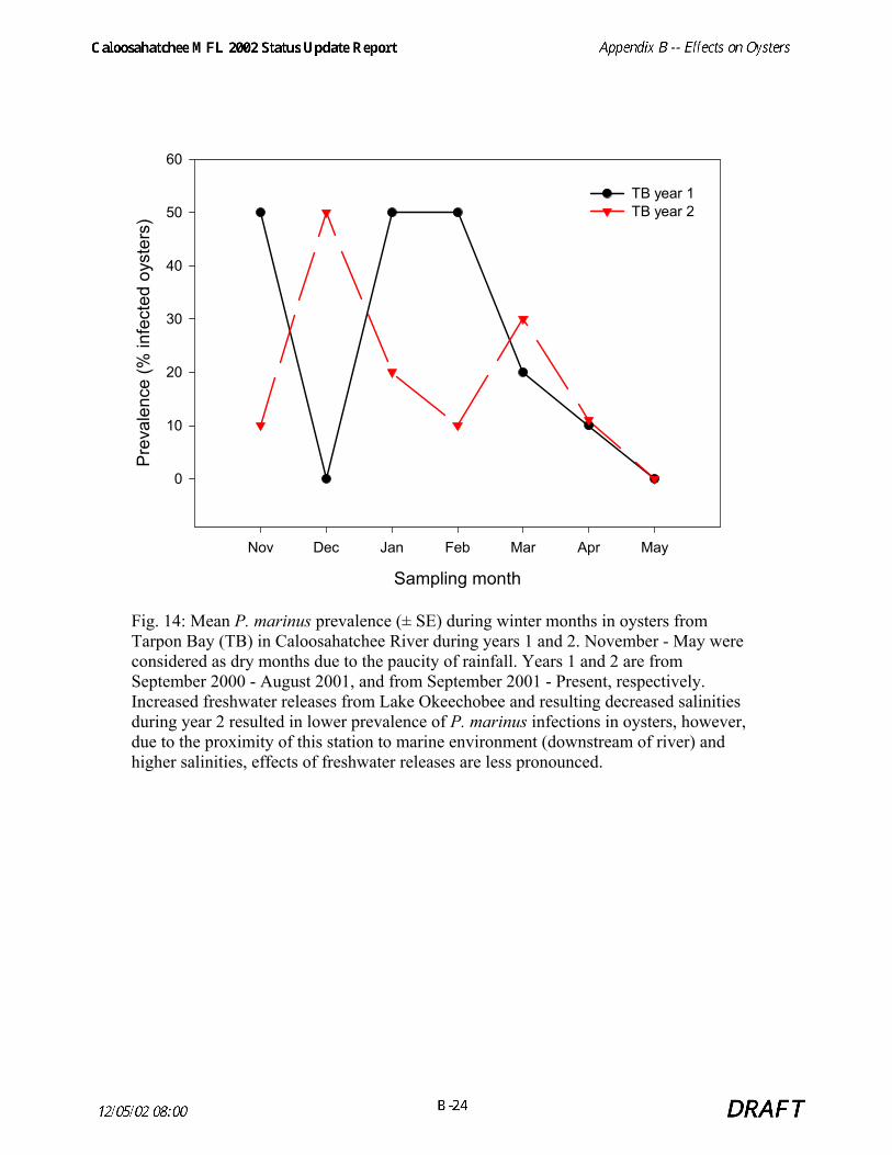
Fig. 14: Mean P. marinus prevalence (± SE) during winter months in oysters from Tarpon Bay (TB) in Caloosahatchee River during years 1 and 2. November - May were considered as dry months due to the paucity of rainfall. Years 1 and 2 are from September 2000 - August 2001, and from September 2001 - Present, respectively. Increased freshwater releases from Lake Okeechobee and resulting decreased salinities during year 2 resulted in lower prevalence of P. marinus infections in oysters, however, due to the proximity of this station to marine environment (downstream of river) and higher salinities, effects of freshwater releases are less pronounced.

Sampling location
PP CD BI KK TB
P. m
arin
us In
tens
ity
0.0
0.5
1.0
1.5
Yr 1 int Yr 2 int
Fig. 15: Mean P. marinus intensity (± SE) during winter months in oysters from Piney Point (PP), Cattle Dock (CD), Bird Island (BI), Kitchel Key (KK), and Tarpon Bay (TB) in Caloosahatchee River during years 1 and 2. November - May were considered as dry months due to the paucity of rainfall. Years 1 and 2 are from September 2000 - August 2001, and from September 2001 - Present, respectively. Ten oysters per month were randomly samples from the sampling locations per month and intensity (Int) of P. marinus (weighted incidence) was analyzed according to Ray 1954. Increased freshwater releases from Lake Okeechobee and resulting decreased salinities resulted in lower infection intensities in oysters from all upstream locations.
Sampling month
Nov Dec Jan Feb Mar Apr May
P. m
arin
us in
tens
ity
-0.1
0.0
0.1
0.2
0.3
0.4
0.5PP year 1 PP year 2
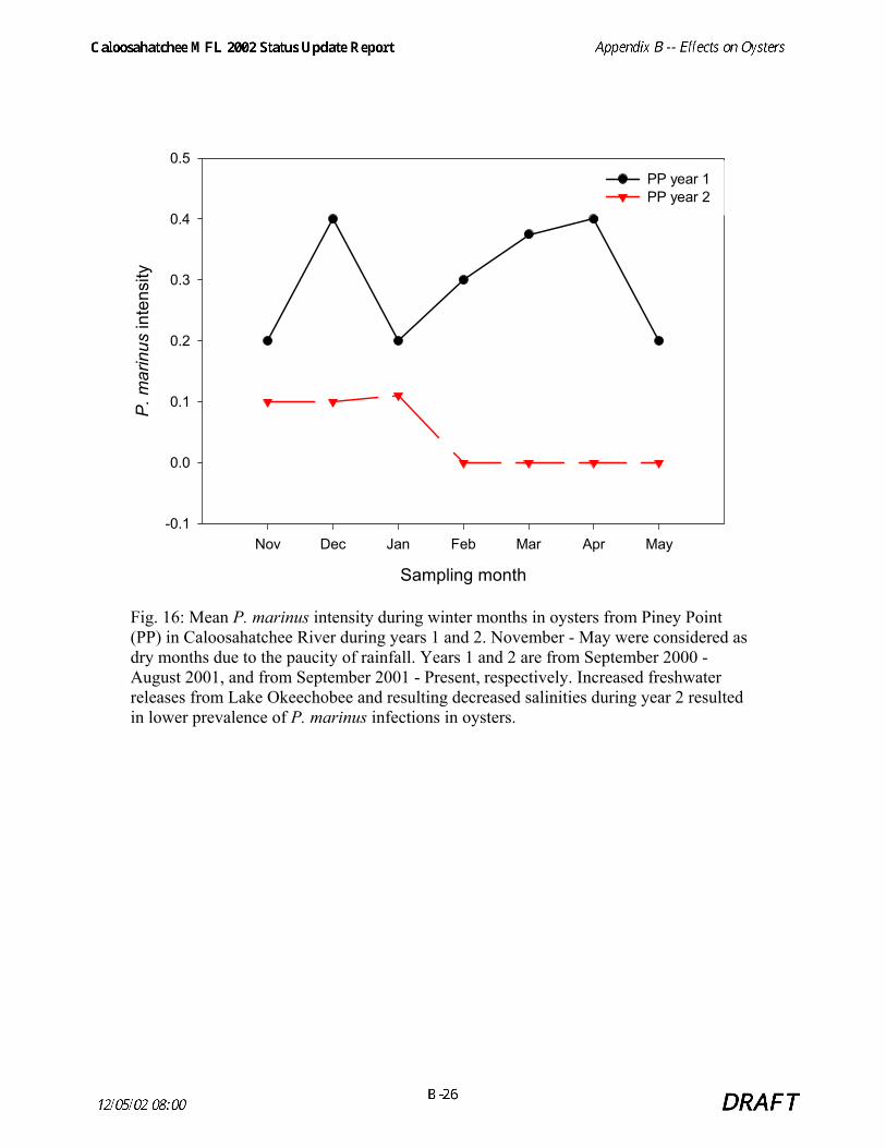
Fig. 16: Mean P. marinus intensity during winter months in oysters from Piney Point (PP) in Caloosahatchee River during years 1 and 2. November - May were considered as dry months due to the paucity of rainfall. Years 1 and 2 are from September 2000 - August 2001, and from September 2001 - Present, respectively. Increased freshwater releases from Lake Okeechobee and resulting decreased salinities during year 2 resulted in lower prevalence of P. marinus infections in oysters.

Sampling month
Nov Dec Jan Feb Mar Apr May
P. m
arin
us in
tens
ity
0
1
2
3
CD year 1 CD year 2
Fig. 17: Mean P. marinus intensity during winter months in oysters from Cattle Dock (CD) in Caloosahatchee River during years 1 and 2. November - May were considered as dry months due to the paucity of rainfall. Years 1 and 2 are from September 2000 - August 2001, and from September 2001 - Present, respectively. Increased freshwater releases from Lake Okeechobee and resulting decreased salinities during year 2 resulted in lower prevalence of P. marinus infections in oysters. Cattle Dock site also receives runoff water from the City of Cape Coral and nearby marinas.

Sampling month
Nov Dec Jan Feb Mar Apr May
P. m
arin
us in
tens
ity
0
1
2
3
BI year 1 BI year 2
Fig. 18: Mean P. marinus intensity during winter months in oysters from Bird Island (BI) in Caloosahatchee River during years 1 and 2. November - May were considered as dry months due to the paucity of rainfall. Years 1 and 2 are from September 2000 - August 2001, and from September 2001 - Present, respectively. Increased freshwater releases from Lake Okeechobee and resulting decreased salinities during year 2 resulted in lower prevalence of P. marinus infections in oysters.

Sampling month
Nov Dec Jan Feb Mar Apr May
P. m
arin
us in
tens
ity
0.0
0.2
0.4
0.6
0.8
1.0
KK year 1 KK year 2
Fig. 19: Mean P. marinus intensity during winter months in oysters from Cattle Dock (CD) in Caloosahatchee River during years 1 and 2. November - May were considered as dry months due to the paucity of rainfall. Years 1 and 2 are from September 2000 - August 2001, and from September 2001 - Present, respectively. Increased freshwater releases from Lake Okeechobee and resulting decreased salinities during year 2 resulted in lower prevalence of P. marinus infections in oysters.

Sampling month
Nov Dec Jan Feb Mar Apr May
P. m
arin
us in
tens
ity
0
1
2
TB year 1 TB year 2
Fig. 20: Mean P. marinus intensity during winter months in oysters from Tarpon Bay (TB) in Caloosahatchee River during years 1 and 2. November - May were considered as dry months due to the paucity of rainfall. Years 1 and 2 are from September 2000 - August 2001, and from September 2001 - Present, respectively. Increased freshwater releases from Lake Okeechobee and resulting decreased salinities during year 2 resulted in lower prevalence of P. marinus infections in oysters, however, due to the proximity of this station to marine environment (downstream of river) and higher salinities, effects of freshwater releases are less pronounced.

Technical Documentation to Support Development ofMinimum Flows and Levels for the Caloosahatchee
River and Estuary
Appendix C
Impacts of Freshwater Inflows on the Distribution ofZooplankton and Ichthyoplankton in the
Caloosahatchee Estuary, FloridaBy Chamberlain, R.H., P.H. Doering, K.M. Haunert, and D. Crean
Contents
Introduction ............................................................................................................................C-1Methods..................................................................................................................................C-1Results....................................................................................................................................C-2
Zooplankton........................................................................................................................C-2Ichthyoplankton ..................................................................................................................C-3
Conclusion..............................................................................................................................C-5Zooplankton........................................................................................................................C-5Ichthyoplankton ..................................................................................................................C-6
Literature Cited.......................................................................................................................C-6
Florida Bay and Lower West Coast DivisionSouthern District Restoration Department
South Florida Water Management District
January 2003

02/03/03 10:53 AM C-2 DRAFT

Caloosahatchee MFL 2002 Status Update Report Appendix C- - Impacts of Freshwater Flows on Plankton
02/03/03 10:53 AM C-1 DRAFT
Impacts of Freshwater Inflows on the Distribution of Zooplankton andIchthyoplankton in the Caloosahatchee Estuary, Florida
byChamberlain, R.H., P.H. Doering, K.M. Haunert, and D. Crean
Introduction
An average monthly freshwater inflow of 300 cfs has been established as the minimum flow and
level (MFL) to protect the upstream freshwater-brackish plant, Vallisneria americana (Figure 1),
from high salinity exposure during the dry season (MFL Document – SFWMD 2000). A
maximum discharge limit of 2,800 cfs has been recommended to protect downstream seagrass
from being adversely impacted by low salinity conditions (Chamberlain and Doering 1998a, b;
Doering et al. 2002). Expert reviewers of the MFL document suggested that further investigation
was needed to understand how the above-recommended inflows influence other biota in the
Caloosahatchee Estuary. This summary paper highlights the results of two data analysis efforts,
previously presented as posters (Chamberlain et al. 1999, 2001), with the following goals: (1)
characterize the spatial and seasonal abundance of zooplankton and ichthyoplankton as it relates
to freshwater inflow; (2) specifically assess the potential influence of above-recommended
discharges on these components of the plankton community; and (3) determine inflows that tend
to maximize abundance.
Methods
Paired 0.5 mm conical zooplankton nets with a 243 micron mesh were obliquely towed from the
stern of a 20’ boat. Another pair of nets with a 505-micron mesh was concurrently deployed
from a side boom to collect ichthyoplanton. The ichthyoplankton nets also proved successful at
collecting fish eggs, shrimp, and crab larvae. A flow meter was affixed in the mouth of one
zooplankton and one ichthyoplankton net. Nocturnal samples were collected monthly at six (6)
stations (Figure 1) and a seventh station in Pine Island Sound every other month during 1986-
1989. Zooplankton only samples were again collected during abnormally high freshwater inflows
in 1998. Net samples were identified to the lowest taxonomic level possible. Repetitive samples
of zooplankton in the water column were also collected with a bilge pump in 1988-1989 at
stations 1, 2, 4, 5 during low to moderate inflows, and again during high inflows in 1994 -1996
and 1998. A fixed volume was filtered through a 60-micron mesh and individual zooplankton

Caloosahatchee MFL 2002 Status Update Report Appendix C- - Impacts of Freshwater Flows on Plankton
02/03/03 10:53 AM C-2 DRAFT
were sorted into major groups and enumerated. Freshwater inflow volume through S-79 was
measured daily throughout the year. Water quality, including salinity, was sampled during each
trip.
Results
Zooplankton
There were 108 invertebrate taxa collected during the 1986-1989 zooplankton net sampling. The
copepod, Acartia tonsa comprised 52% of the total density. In the pump samples, copepod
nauplii and all other copepod stages constituted 67% of the zooplankton, contributing 45% and
22% respectively. Over 90% of the crab and shrimp larvae in the ichthyoplankton nets were
Minippe mercenaria (stone crabs). Penaeus sp. comprised approximately 7% and Callinectes sp.
accounted for approximately 2%.
In general, mean zooplankton density (net samples) increased with increasing distance from S-
79. Statistical differences, as judged by a multiple range test, are shown in Figure 2 (bottom).
The greatest zooplankton density occurred at higher salinity stations (> 20ppt) farthest from S-
79. A similar trend appeared for the pump samples, however not as strongly, with station 5
supporting the least zooplankton density.
Stations 5 and 6 accounted for over 99% of the shrimp and crab larvae enumerated in the
ichthyoplankton nets. The peak abundance occurred at station 6 where salinity was nearly the
highest. Blue crab larvae (Callinectes sapidus) require salinity above 20 ppt, demonstrating the
importance of establishing a maximum discharge limit for station 6.
There were apparent differences in density between seasons at each station during both pump
and net sampling (Figure 3). This was most evident in the pump samples, with the period of
April – July being the most productive, followed by December – March. Zooplankton density
was lowest during the rainiest portion of wet season, August – November. A similar, but less
evident seasonal influence can be seen in the net samples. The same order of seasonal ranking
appears (April – July and December – March > the August – November), but only at stations 3,
4, and 5. Seasonal influences become less clear at the estuarine boundaries.

Caloosahatchee MFL 2002 Status Update Report Appendix C- - Impacts of Freshwater Flows on Plankton
02/03/03 10:53 AM C-3 DRAFT
Inflow volume appears to be more of an influence than salinity. Density decreases as inflows
increase at most stations for both pump and net samples, as shown in Figure 4. In zooplankton
net samples, inflows that exceed 1,500 cfs and approach 3,000 cfs or greater are associated with
the lowest zooplankton density, except at the farthest downstream stations (6 and 7).
In zooplankton net samples, the average density for all stations combined were further separated
into 6 inflow categories and tested for significant differences (Figure 5). Optimal inflows
associated with the highest zooplankton densities occurred in the 150-600 cfs range. Flows
higher or lower than this were associated with lower densities. Inflows that approach and exceed
1,200 cfs supported the least zooplankton density.
Again in the zooplankton net samples, the same 6 flow categories were used to examine the
influence of freshwater input at each station (Figure 6). Except at station 6, the same general
trend appears for most stations as was seen when flow was examined for all stations combined.
Inflows that approach and exceed 2,500 cfs were associated with the least zooplankton; and
inflows in the 2nd and usually 3rd categories (151 - 600 cfs) always supported the greatest
density of zooplankton.
Ichthyoplankton
Average monthly discharges from S-79 ranged from 69 to 4,510 cfs during 1986-1989 (Figure
7). These inflows were highly variable between months and years. Average discharge was <
1,000 cfs during January through June, but approached 2,000 cfs during the remaining six
months. High variability in discharge resulted in wide fluctuations in salinity, with a range >20
ppt (Figure 8) at Stations 3, 4, and 5.
Five fish families contributed > 1% to the total fish abundance. Engraulidae, Gobiidae,
Sciaenidae, Clupeidae and Blennidae accounted for approximately 96% of the total abundance.
Anchoa mitchelli was the dominant single species comprising 54% of the number of fish
collected. Fish egg composition was dominated by Engraulids, with Sciaenids also making a
significant contribution.
As with inflow and salinity, the average ichthyoplankton density was highly variable between
stations (Figure 9). The distribution pattern generally followed that of Anchoa. The median

Caloosahatchee MFL 2002 Status Update Report Appendix C- - Impacts of Freshwater Flows on Plankton
02/03/03 10:53 AM C-4 DRAFT
density followed the longitudinal salinity distribution as did average density to a lesser extent.
Significant differences between stations also followed the median values. Station 6 was
associated with the greatest density, station 5 ranked 2nd, and Station 2 was associated with the
lowest density. The density of fish eggs generally followed the same patterns of distribution and
significance as the ichthyoplankton.
The average ichthyoplankton density was greater for most of the estuary during the spring
months, March through June (Figure10). This is when inflow is usually lower (Figure7). The
high density at Station 3 during November through February was primarily due to a high
abundance of Anchoa mitchelli that occurred late in February 1986. High ichthyoplankton
density occurred during July through October only at Station 6. During this time period,
discharges are usually greater (Figure 7). It is likely that Station 6 offers better salinity conditions
for most species than upstream when discharges are high.
Average egg density is also greatest during spring, for both Engraulids and Sciaenids (Figure
11). November through February produced the 2nd highest abundance. Anchovies prefer
spawning upstream of Shell Point at Stations 4 and 5 during the dry season, November –June.
As with ichthyoplankton, Engraulid egg density (Figure 11a) increases downstream at station 5
and 6 during the wet season, July – October. Average Sciaenid egg density (Figure 11b) also was
greatest during spring, but remained high at Station 6 during this season, compared to declining
trend of Engraulid eggs. Sciaenids generally seem to prefer spawning farther down stream
in higher salinity water, which is especially evident as seasonal freshwater inflows increased
during the wet season.
Analysis of data at each station determined that when inflows were < 600 cfs, ichthyoplankton
density was significantly greater at Stations 3, 4, and 5. The same was true for eggs, except at
Station 2, where inflows < 600 cfs also were associated with greater density. No significant
differences in densities associated with inflows were found at the remaining stations.
During the dry season (November – June) is when the estuary is most likely to suffer a lack of
minimum flows to support upstream submerged plants, but also most threatened by large Lake
Okeechobee regulatory releases. When the dry season was examined separately during this

Caloosahatchee MFL 2002 Status Update Report Appendix C- - Impacts of Freshwater Flows on Plankton
02/03/03 10:53 AM C-5 DRAFT
analysis, inflows that exceeded 2,500 cfs were associated with the lowest ichthyoplankton and
egg density and inflows < 600 cfs had greater densities.
Inflows were consistently lower during the spring months of 1989 than during 1987 and 1988.
Since spring is the most productive time in the estuary, extra sampling was conducted in March
and April during each of these three years. During 1987 and 1988 freshwater inflows averaged
1,836 and 1,854 cfs, while in 1989 the mean inflow was 433 cfs. In 1989, ichthyoplankton
density was greater in the estuary, especially upstream of Shell Point (Figure 12). More of the
estuary also was used for spawning during 1989 (Figure 13). This suggest that lower flows favor
increased utilization of the estuary.
Conclusion
Zooplankton
Mean zooplankton density increased along with salinity and distance from S-79. The late spring
to early summer season is generally when zooplankton density is greatest, just prior to the wet
season's heaviest rainfall runoff during August to November when density is lowest. High
freshwater inflows and lower salinity drive zooplankton down regardless of the season.
Zooplankton were weakly related to salinity, but correlated well with freshwater inflow volume,
possibly due to a "wash out" effect.
Some freshwater inflow is important to the estuary in order for zooplankton to achieve maximum
density. At most stations, except those farthest downstream (6 and 7) the greatest densities were
measured when inflows range was150-600 cfs. Except at station 6, inflows that exceed 1,200-
1,500 cfs were associated with reduced zooplankton density. Inflows that were greater than
2,500-3,000 cfs supported the lowest density.
Ninety percent of the shrimp and crab larvae were collected at station 5 and 6, with the peak
abundance occurring at station 6, when salinity exceeded 20-25 ppt. Therefore inflows that
normally do not exceed 2,500 -3,000 cfs will protect the San Carlos Bay spawning and rearing
area. Inflows that remain below 1,200-1,500 cfs will also provide habitat upstream of Shell
Point.

Caloosahatchee MFL 2002 Status Update Report Appendix C- - Impacts of Freshwater Flows on Plankton
02/03/03 10:53 AM C-6 DRAFT
Ichthyoplankton
Freshwater inflows < 600 cfs were associated with the highest ichthyoplankton and egg density.
The maximum ichthyoplankton utilization of the estuary and spawning occurred in more areas
during low flows. Ichthyoplankton and eggs were greatest during the dry season, especially in
spring. Dry season and spring minimum inflows necessary to protect upstream SAV will not
adversely impact ichthyoplankton and egg abundance. Inflow < 600-800 cfs, associated with
higher seagrass production near Station 5 (Doering et al. 2002), should also maximize
ichthyoplankton and egg abundance in this region and downstream.
Literature Cited
Chamberlain, R. H. and P.H. Doering. 1998a. Freshwater inflow to the Caloosahatchee Estuaryand the resource-based method for evaluation, p. 81-90. In S.F. Treat (ed.), Proceedingsof the 1997 Charlotte Harbor Public Conference and Technical Symposium. SouthFlorida Water Management District and Charlotte Harbor National Estuary Program,Technical Report No. 98-02. Washington, D.C.
Chamberlain, R. H. and P.H. Doering. 1998b. Preliminary estimate of optimum freshwaterinflow to the Caloosahatchee Estuary: A resource-based approach, p. 121-130. In S.F.Treat (ed.), Proceedings of the 1997 Charlotte Harbor Public Conference and TechnicalSymposium. South Florida Water Management District and Charlotte Harbor NationalEstuary Program, Technical Report No. 98-02. Washington, D.C.
Chamberlain, R.H., P.H. Doering, K.M. Haunert, and D. Crean. 2001. Distribution ofichthyoplankton and recommended freshwater inflow to the Caloosahatchee Estuary, FL.Poster presentation, 16th Biennial Conference of the Estuarine Research Federation.
Chamberlain, R.H., P.H. Doering, K.M. Haunert, and D. Crean. 1999. Distribution ofzooplankton and recommended freshwater inflow to the Caloosahatchee Estuary, FL.Poster presentation, 15th Biennial Conference of the Estuarine Research Federation.
Doering, P.H., R.H. Chamberlain, and D.E. Haunert. 2002. Using submerged aquatic vegetationto establish minimum and maximum freshwater inflows to the Caloosahatchee Estuary(Florida). Estuaries (In Press).
South Florida Water Management District (SFWMD). 2000. Technical document to supportdevelopment of minimum flows and levels for the Caloosahatchee River and Estuary.

Caloosahatchee MFL 2002 Status Update Report Appendix C- - Impacts of Freshwater Flows on Plankton
02/03/03 10:53 AM C-7 DRAFT
FIGURES
Figure 1. Plankton sampling stations and locations of submerged vegetation found upstream ofShell Point in the Caloosahatchee Estuary, southwest Florida.
Figure 2. Average zooplankton density per station and the corresponding mean salinity duringnet sampling. Letters associated with net samples summarize results of a multiple range testexamining potential differences between stations. Bars with different letters are significantlydifferent (p<0.05).
Figure 3. Average zooplankton density at each station compared to seasonal differences.
Figure 4. Influence of freshwater inflow through S-79 on zooplankton density at downstreamestuary stations.
Figure 5. Effect of freshwater inflow through structure S-79 on net collected zooplanktondensity. Letters summarize results of a multiple range test examining potential differencesbetween inflow categories. Bars with different letters are significantly different (p<0.05).Figure 6. Effect of freshwater inflow through structure S-79 on net collected zooplankton density at six downstreamstations. Letters summarize results of a multiple range test examining potential differences between inflowcategories. Bars with different letters are significantly different (p<0.05).
Figure 7. Average monthly freshwater inflows from S-79 during sampling. Inflows groupedtogether in two-month intervals. Inflow range and median for each interval indicated.
Figure 8. Salinity distribution at each sampling station during ichthyoplankton sampling.Salinity range and median value indicated.
Figure 9. Average and median ichthyoplankton density at each station during the entire period ofsampling. Average salinity at each station also indicated. The number above the bars is thecoefficient of variation. Bars with different letters are significantly different (p<0.05).
Figure 10. Average ichthyoplankton and coefficient of variation (CV) at sampling stationsduring three seasons.
Figure 11. Average fish egg density at sampling stations during three seasons for: (a) Engraulidsand (b) Sciaenids.
Figure 12. Average ichthyoplankton density at each sampling station during three consecutivespring seasons experiencing different freshwater inflow conditions.
Figure 13. Average fish egg density at each sampling station during three consecutive springseasons experiencing different freshwater inflow conditions.

Caloosahatchee MFL 2002 Status Update Report Appendix C- - Impacts of Freshwater Flows on Plankton
02/03/03 10:53 AM C-8 INTERNAL DRAFT

Caloosahatchee MFL 2002 Status Update Report Appendix C- - Impacts of Freshwater Flows on Plankton
02/03/03 10:53 AM C-9 INTERNAL DRAFT
Pump CollectedD
ensi
ty (
m-3
)
Net Collected
Station
Den
sity
(m
-3)
0
2000
4000
6000
8000
10000
12000
14000
16000
18000
Sal
inity
(pp
t)
0
5
10
15
20
25
30
35
Average zooplankton density per station Average salinity per station
250000
200000
150000
100000
50000
1 2 3 4 5 6 7
1 2 3 4 5 6 7
A
AB
B
C
DD
0
Figure 2

Caloosahatchee MFL 2002 Status Update Report Appendix C- - Impacts of Freshwater Flows on Plankton
02/03/03 10:53 AM C-10 DRAFT
Pump CollectedD
ensi
ty (
m-3
)
Net Collected
Station
Den
sity
(m-3
)
0
5000
10000
15000
20000
Average zooplankton density during all seasonsApril - JulyAugust - NovemberDecember - March
300,000
250,000
200,000
150,000
100,000
50,000
1 2 3 4 5 6 7
1 2 3 4 5 6 7
0
Figure 3

Caloosahatchee MFL 2002 Status Update Report Appendix C- - Impacts of Freshwater Flows on Plankton
02/03/03 10:53 AM C-11 DRAFT
Net Samples
Stations
0 1 2 3 4 5 6
Den
sity
(m
-3 )
0
5000
10000
15000
20000
25000
Average zooplankton during freshwater inflows < 500 cfsDensity during inflows 500 - 1,500 cfsDensity during inflows 1,500 - 3,000 cfsDensity during inflows > 3,000 cfs
50000
100000
150000
200000
250000
300000
350000
0
Figure 4
Pump Samples
0 1 2 3 4 5 6
Den
sity
(m
-3 )

Caloosahatchee MFL 2002 Status Update Report Appendix C- - Impacts of Freshwater Flows on Plankton
02/03/03 10:53 AM C-12 DRAFT
Average Zooplankton Density per Freshwater Inflow Category
Freshwater Inflow Categories
Den
sity
(m
-3)
0
2000
4000
6000
8000
10000
12000
14000
16000
1 2 3 4 5 60-150 cfs
(151-300 cfs)(301-600 cfs)
(601-1200 cfs)
(1201-2500 cfs)(>2500 cfs)
A
A
B B
C
C
(cubic feet per second)
(Net Samples: All Stations Combined)
Figure 5

Caloosahatchee MFL 2002 Status Update Report Appendix C- - Impacts of Freshwater Flows on Plankton
02/03/03 10:53 AM C-13 DRAFT
a. Station 1 Net Samples
1 2 3 4 5 6
Den
sity
(m
-3 )
0
3000
6000
9000
12000
15000
18000
21000
24000
b. Station 2 Net Samples
1 2 3 4 5 6
Den
sity
(m
- 3 )
0
3000
6000
9000
12000
15000
18000
21000
24000
c. Station 3 Net Samples
1 2 3 4 5 6
Den
sity
(m
- 3 )
0
3000
6000
9000
12000
15000
18000
21000
24000
d. Station 4 Net Samples
1 2 3 4 5 6
Den
sity
(m
-3 )
0
3000
6000
9000
12000
15000
18000
21000
24000
e. Station 5 Net Samples
Freshwater Inflow Categories (cubic feet per second)
1 2 3 4 5 6
Den
sity
(m
- 3 )
0
3000
6000
9000
12000
15000
18000
21000
24000
f. Station 6 Net Samples
Freshwater Inflow Categories (cubic feet per second)
1 2 3 4 5 6
Den
sity
(m
-3 )
0
3000
6000
9000
12000
15000
18000
21000
24000
(0-150 cfs)(151-300 cfs)
(301-600 cfs)(601-1200 cfs)
(1201-2500 cfs)(>2500 cfs)
(0-150 cfs)(151-300 cfs)
(301-600 cfs)(601-1200 cfs)
(1201-2500 cfs)(>2500)
A
A
AB ABB B
A
B
BC BC C C
AA A
B BC
AA
B
BC
CC
* No significant difference between flow categoriesA
AB AB
AB AB
B
Figure 6

Caloosahatchee MFL 2002 Status Update Report Appendix C- - Impacts of Freshwater Flows on Plankton
02/03/03 10:53 AM C-14 DRAFT
Temporal Inflow Categories; 1986-1989
Two-Month Inflow Categories
Inflo
w (
ft3 s
ec-1
: cf
s)
0
1000
2000
3000
4000
5000
Box and Wisker Plots for Two Month Flow Intervals
Average Freshwater Inflows
Jan-FebMar-Apr
May-JuneJuly-Aug
Sep-OctNov-Dec
95 Percentile
75 Percentile
Median
25 Percentile 5 Percentile
Outlier
Figure 7

Caloosahatchee MFL 2002 Status Update Report Appendix C- - Impacts of Freshwater Flows on Plankton
02/03/03 10:53 AM C-15 DRAFT
Salinity Distribution
Sampling Stations
1 2 3 4 5 6 7
Sal
init
y (p
pt)
0
10
20
30
40
Plots for Salinity Range
95 Percentile
Median
25 Percentile
5 Percentile
75 Percentile
Outlier
Figure 8

Caloosahatchee MFL 2002 Status Update Report Appendix C- - Impacts of Freshwater Flows on Plankton
02/03/03 10:53 AM C-16 DRAFT
Ichthyoplankton Density
Sampling Station
1 2 3 4 5 6 7
Den
sity
(m
-3 )
0
1
2
3
4
5
6
7
Sal
inity
(p
pt)
0
5
10
15
20
25
30
35
Average Ichthyoplankton DensityMedian DensityAverage Salinity
BC C
BC BC
AB
A
1.53 1.55
12.79 15.05
3.56
6.38
2.77
CV =
Figure 9

Caloosahatchee MFL 2002 Status Update Report Appendix C- - Impacts of Freshwater Flows on Plankton
02/03/03 10:53 AM C-17 DRAFT
Average Ichthyoplankton Density During Three Seasons
Station
1 2 3 4 5 6
Den
sity
(m
-3 )
0
1
2
3
4
5
6
7
8
9
10
11
12Ichthyoplankton density during November through FebruaryDensity during March through JuneJuly through October
CV
Figure 10

Caloosahatchee MFL 2002 Status Update Report Appendix C- - Impacts of Freshwater Flows on Plankton
02/03/03 10:53 AM C-18 DRAFT
b. Average Sciaenid Egg Density
1 2 3 4 5 6
Den
sity
(m
-3 )
0
10
20
30
40
50
60
160
170
180
190
200
a. Average Engraulid Egg Density
1 2 3 4 5 6
Den
sity
(m
-3 )
0
20
40
60
80
100
120
140
160
180
200
November though FebruaryMarch through JuneJuly through October
Station
Figure 11
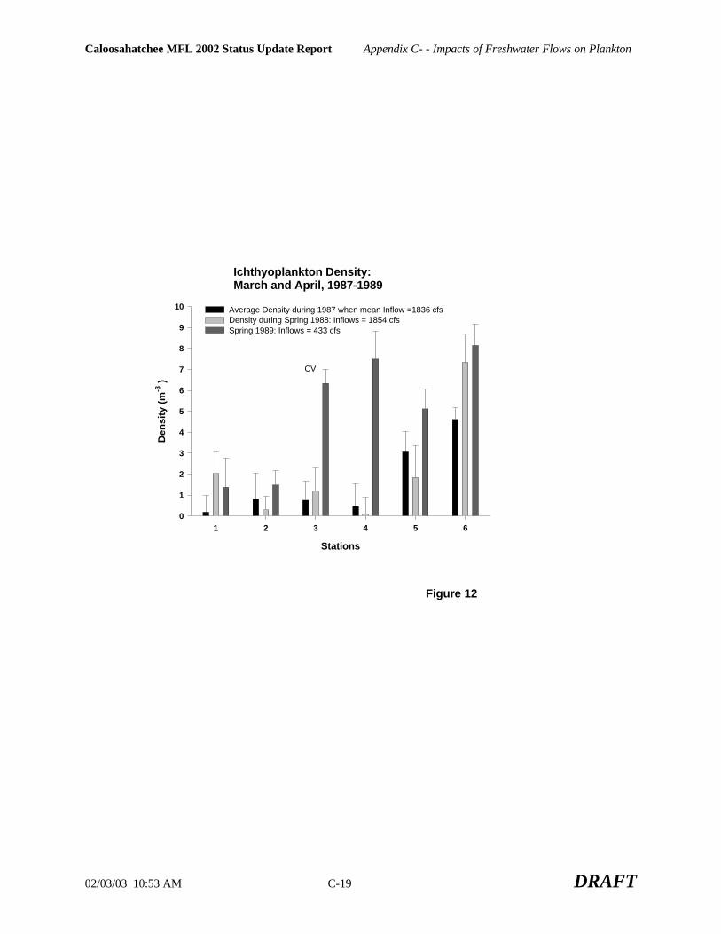
Caloosahatchee MFL 2002 Status Update Report Appendix C- - Impacts of Freshwater Flows on Plankton
02/03/03 10:53 AM C-19 DRAFT
Ichthyoplankton Density: March and April, 1987-1989
Stations
1 2 3 4 5 6
Den
sity
(m
-3 )
0
1
2
3
4
5
6
7
8
9
10 Average Density during 1987 when mean Inflow =1836 cfsDensity during Spring 1988: Inflows = 1854 cfsSpring 1989: Inflows = 433 cfs
CV
Figure 12

Caloosahatchee MFL 2002 Status Update Report Appendix C- - Impacts of Freshwater Flows on Plankton
02/03/03 10:53 AM C-20 DRAFT
Fish Egg Density:March and April, 1987-1989
Stations
1 2 3 4 5 6
Den
sity
(m
-3 )
0255075
100125150175200225250275300325350375400425450 Average Egg Density during 1987 when mean Inflow = 1836
Egg Density during Spring 1988: Inflows = 1854 Spring 1989: Inflows = 433 cfs
Figure 13

02/03/03 10:35 AM D-1 DRAFT
Technical Documentation to Support Development ofMinimum Flows and Levels for the Caloosahatchee
River and Estuary
Appendix D
Salinity Tolerance of Vallisneria and Salinity Criteria P.H. Doering
Contents
Introduction ............................................................................................................................D-1Methods..................................................................................................................................D-1
Salinity Tolerance of Vallisneria .........................................................................................D-1Results....................................................................................................................................D-3
Salinity Tolerance of Vallisneria .........................................................................................D-3Effect of Discharge on Density of Plants in the Field...........................................................D-3
Discussion ..............................................................................................................................D-4knowledgements .....................................................................................................................D-5Literature Cited.......................................................................................................................D-6Species....................................................................................................................................D-8
Florida Bay and Lower West Coast DivisionSouthern District Restoration Department
South Florida Water Management District
January 2003

02/03/03 10:35 AM D-2 DRAFT
Caloosahatchee MFL 2002 Status Update Report Appendix D - Salinity Tolerance and Salinity Criteria
02/03/03 10:35 AM D-1 DRAFT
Salinity Tolerance of Vallisneria and Salinity Criteria
Introduction
The Caloosahatchee MFL rule includes two salinity criteria. An exceedance occurs (1) if
the 30-day moving average salinity at Ft Myers exceeds 10 ppt and (2) if a single daily
average salinity exceeds 20 ppt. The research program initiated in response to the
scientific peer review has generated new laboratory and field data on the salinity
tolerance of V. americana. In this report data are analyzed to determine if these threshold
salinities are still supported. The technical criteria also state that a flow of 300 cfs is
necessary to maintain Vallisneria in the upper estuary. Data from our field monitoring
program are analyzed to determine if this flow is supported.
Methods
Salinity Tolerance of Vallisneria
Salinity tolerance was determined both from an analysis of monitoring of field
populations and from laboratory mesocosm experiments designed to measure the effects
of salinity on growth and mortality. Detailed descriptions of laboratory methods may be
found in Doering et al. 1999, Doering and Chamberlain 2000, and Doering et al. 2001. A
brief description appears below.
V. americana collected from the Caloosahatchee, was planted in rectangular tubs (14 cm
H x 24 cm L x 15 cm W) containing sediment from the site of collection. Initially, tubs
contained 4 to 8 shoots. Tubs and plants were distributed among ten cylindrical
mesocosm tanks (1.3 m in diameter x 1 m deep, n=4 to 6 tubs/tank depending on the
experiment) filled with water to a depth of 60 cm (volume=800 l). The tanks were located
indoors at an aquarium facility at the Gumbo Limbo Nature Center in Boca Raton, FL. A
1000 Watt metal halide lamp, kept on a L:D photoperiod of 12:12 h, supplied light to
each tank.
Caloosahatchee MFL 2002 Status Update Report Appendix D - Salinity Tolerance and Salinity Criteria
02/03/03 10:35 AM D-2 DRAFT
A given salinity was maintained by mixing appropriate volumes of fresh and salt water
(total volume=114 l) from each of two head tanks located above each mesocosm. Head
tanks were alternately filled and emptied into the mesocosms using solenoid valves
controlled by timers. Thus, water was delivered to the mesocosms in a series of 114-liter
pulses. Water in the mesocosms was replaced 3 times daily. Salt water was pumped
from the Atlantic Ocean. Tap water, passed through a series of activated charcoal towers
and filters (20 micron pore size) to remove chlorine, was used as a source of fresh water.
The net growth data summarized in this report was collected during 4 experiments
conducted between 1996 and 2001 (Table D-1). Plants were exposed to constant salinity
treatments (n=two mesocosms per treatment) for periods of 3 to 10 weeks. The exact
salinity treatments depended on whether the purpose of the experiment was to measure
growth at low salinity or tolerance to high salinity. Numbers of blades and shoots were
counted on a weekly basis. These weekly measurements were used to determine net
(production – loss) rates of blade and shoot growth. Data taken on a given day in each
mesocosm were averaged across tubs, yielding two data points per treatment per week of
the experiment. Net growth was modeled using the exponential growth equation (Nt =
N0ert) were N0 is the number of blades or shoots at the beginning of exposure and Nt is
the number after t days.
A program to monitor V. americana on a monthly basis at Stations 1 - 4 (Figure D-1)
was instituted in 1998. At each station, a pair of 100-m transects (one parallel to shore,
one perpendicular to shore) was established at two sites. On each sampling date the
number of blades and shoots was counted in 5 0.1 m2 quadrats placed randomly along
each transect (n=5 quadrats per transect, n=10 quadrats per site, n=20 quadrats per
station). A detailed analysis of the first year of data may be found in Bortone and Turpin
(2000). Data reported here encompass the time period January 1998 – April 2001.
Both field and laboratory data were used to select tolerable salinity thresholds that could
be used to calculate minimum and maximum flows (see above). Field salinity tolerances
were identified from plots of plant density as a function of salinity on the day of
sampling. Tolerable, threshold salinities were those associated with marked or rapid

Caloosahatchee MFL 2002 Status Update Report Appendix D - Salinity Tolerance and Salinity Criteria
02/03/03 10:35 AM D-3 DRAFT
changes in plant density. Laboratory data were examined to identify a range of salinity
where growth was low, and close to zero. Using non-linearities to identify thresholds is
common in methods used to determine flow requirements for streams and rivers (Estevez
2000b).
Results
Salinity Tolerance of Vallisneria
For V. americana, the net growth rates of shoots and blades in the laboratory decreased as
salinity increased, with mortality occurring at salinities greater than 15 o/oo (Figure D-
2). At 18 o/oo a 50% loss of shoots would occur in 38 days. At 20 o/oo a 50% loss
would occur in 16 days. In the region between 10 o/oo and 15 o/oo , the change in
growth in response to a change in salinity was very small. This lack of response was
especially evident for the number of blades: growth rates at 10 o/oo and 15 o/oo were
virtually identical. In this zone, plants survived but net growth rates of shoots and blades
were low and relatively unchanging.
Data from field monitoring agreed well with results from the laboratory (Figure D-3,
upper panel). The distribution of points in the four quadrants defined by the reference
lines on the graph of shoot density and salinity may be treated as cells in a 2 x 2
contingency table. Higher densities in the field (> 400 shoots m-2) occurred at salinities
less than about 10 o/oo. Lower densities (< 400 shoots m-2) were more frequent at
salinities above 10 o/oo (Figure D-3, upper panel, X2 = 4.53, p<0.05 ).
Effect of Discharge on Density of Plants in the Field
To investigate the potential effects of discharge on Vallisneria in the upper estuary, plant
density data collected during the monitoring program was plotted as a function of the
average discharge at S-79 for the 30 days prior to sampling. Field monitoring data
indicated that higher shoot densities (> 400 m-2) occur at 30-day average discharges
greater than 8.5 m3 sec-1 (300 cfs) (Figure D-5, X2 = 7.98, p<0.01).

Caloosahatchee MFL 2002 Status Update Report Appendix D - Salinity Tolerance and Salinity Criteria
02/03/03 10:35 AM D-4 DRAFT
Discussion
The use of marine and estuarine SAV for management purposes appears to be a well-
accepted practice (Batiuk et al. 1992; Dennison et al. 1993; Stevenson et al. 1993;
Tomasko et al. 1996; Johansson and Greening 2000; Virnstein and Morris 2000). This
stems in part from their sensitivity to pollutants of interest (e.g. nutrients, Tomasko et al.
1996) and in part from their ecological significance.
Although V. americana is considered a freshwater species, it is salt tolerant. Salinity
tolerances of V. americana reported in the literature vary (Doering et al. 1999). Bourn
(1932; 1934) found that growth declined with increasing salinity until it ceased at 8.4 o/oo.
Haller et al. (1974) reported growth at 3.33 o/oo , no growth at 6.66 o/oo or 10 o/oo and death
at 13.3 o/oo . After 5 weeks, Twilley and Barko (1990) found no effect of salinity on
growth over the range 0 o/oo to 12 o/oo. Our laboratory results suggest that for V.
americana from the Caloosahatchee, growth is low or nil in the 10 o/oo – 15 o/oo range with
mortality occurring at salinities greater that 15 o/oo . This agrees well with transplant
experiments conducted in the Caloosahatchee that indicated mortality at salinities greater
than 15 o/oo (Kraemer et al. 1999). Adair et al. (1994) found the distribution of V.
americana in Trinity Bay, Texas limited to salinities less than 10 o/oo . In outdoor
mesocosm experiments, French (2001) observed minimal growth of Vallisneria from the
Chesapeake Bay at 10 o/oo and 15 o/oo .
The combination of results from field monitoring and laboratory experiments conducted
by District and other investigators agree that 10 o/oo is a critical threshold salinity for
growth. The thirty day averaging period is consistent with laboratory experiments which
show that Vallisneria can survive exposure to 10 o/oo for periods exceeding a month
(Doering et al. 1999; French 2001).
The daily average salinity limit of 20 o/oo was included in the rule to avoid acute
exposure to high salinity. Laboratory experiments (1/5/1998, Table 1) showed that
mortality occurs after a 20 day exposure to 18 o/oo . Shorter exposure (1, 5, or 11 days)
retarded growth but did not cause mortality (Doering et al. 2001). Recently completed
experiments (5/20/2001, Table 1) suggest that a 50 % loss of shoots would occur after 16
Caloosahatchee MFL 2002 Status Update Report Appendix D - Salinity Tolerance and Salinity Criteria
02/03/03 10:35 AM D-5 DRAFT
days of exposure to 20 o/oo. At the earliest, mortality began after 3 days exposure to 20
ppt (One-way ANOVA, p<0.05, Figure D-4). Therefore, a one day exposure to 20 ppt
appears to be a reasonable limit for acute exposure.
Mean monthly flows less than 300 cfs are associated with low densities in the field
(Figure D-3). These monitoring data indicate that 300 cfs should maintain Vallisneria in
the upper Caloosahatchee estuary.
Acknowledgements
For all the help in the laboratory and field the authors thank Callie McMunigal, Matthew
Crane and George Jones from Florida Atlantic University, Keith Donohue and Michael
McMunigal from Harbor Branch Oceanographic Institution, and Kathleen Haunert and
Julian DiGialleonardo from the South Florida Water Management District.

Caloosahatchee MFL 2002 Status Update Report Appendix D - Salinity Tolerance and Salinity Criteria
02/03/03 10:35 AM D-6 DRAFT
Literature Cited
Adair, S.E., J.L. Moore and C.P Onuf 1994. Distribution and status of submergedvegetation in estuaries of the Upper Texas Coast. Wetlands 14: 110-121.
Batiuk, R.A., R.J. Orth, K.A. Moore, W.C. Dennison, J.C. Stevenson, L.W. Staver, V.Carter, N.B. Rybicki, R.E. Hickman, S. Kollar, S. Bieber, and P. Heasly 1992.Chesapeake Bay submerged aquatic vegetation habitat requirements andrestoration targets: A technical synthesis. Chesapeake Bay Program CBP/TRS83/92.
Bortone, S. A. and R. K. Turpin. 2000. Tapegrass life history metrics associated withenvironmental variables in a controlled estuary. p. 65-79. In S.A. Bortone (ed.),Seagrass monitoring, ecology, physiology and management. C. R. C. Press, BocaRaton, Florida.
Bourn, W.S. 1932. Ecological and physiological studies on certain aquatic angiosperms.Contributions From Boyce Thompson Institute 4: 425 - 496.
Bourn, W.S. 1934. Sea-water tolerance of Vallisneria spiralis L. and Potomogetonfoliosus Raf. Contributions From Boyce Thompson Institute 6: 303 - 308.
Dennison, W.C., R.J. Orth, K.A. Moore, J.C. Stevenson, V. Carter, S. Kollar, P. W.Bergstrom and R.A. Batiuk. 1993. Assessing water quality with submersedaquatic vegetation. Bioscience 43:86-94.
Doering, P.H., R.H. Chamberlain, K.M. Donohue, and A.D. Steinman 1999. Effect ofsalinity on the growth of Vallisneria americana Michx. from the CaloosahatcheeEstuary, Florida. Florida Scientist 62(2): 89-105.
Doering, P.H. and R.H. Chamberlain 2000. Experimental studies on the salinitytolerance of turtle grass Thalassia testudinum. p. 81-97, In S.A. Bortone (ed.),Seagrass: Monitoring ecology, physiology, and management. CRC Press (BocaRaton, FL).
Doering, P.H., R.H. Chamberlain and J. M. McMunigal 2001. Effects of simulatedsaltwater intrusions on the growth and survival of Wild Celery, Vallisneriaamericana, from the Caloosahatchee Estuary (South Florida). Estuaries 24: 894-903.
Estevez, E.D. 2000. A review and application of literature concerning freshwater flowmanagement in riverine estuaries. Mote Marine Laboratory Technical ReportNumber 680. Mote Marine Laboratory, Sarasota, Florida.
French, G. T. 2001 Effects of light and salinity stress on Vallisneria americana (wildCelery). Master of Science Thesis, School of Marine Science, College of Williamand Mary in Virginia. 137pp.
Haller, W.T., D. L. Sutton, and W. C. Barlowe. 1974. Effects of salinity on growth ofseveral aquatic macrophytes. Ecology 55: 891-894

Caloosahatchee MFL 2002 Status Update Report Appendix D - Salinity Tolerance and Salinity Criteria
02/03/03 10:35 AM D-7 DRAFT
Johansson, J.O.R. and H. S. Greening. 2000. Seagrass restoration in Tampa Bay: Aresource-based approach to estuarine management. p. 279-294. In S.A.Bortone(ed.), Seagrasses: Monitoring, ecology, physiology and management. CRC Press,Boca Raton Fl.
Kraemer, G. P., R. H. Chamberlain, P. H. Doering, A. D. Steinman, and M. D. Hanisak.1999. Physiological response of transplants of the freshwater angiospermVallisneria americana along a salinity gradient in the Caloosahatchee Estuary(SW Florida). Estuaries 22: 138-148.
Stevenson, J. C., L.W. Staver and K.W. Staver. 1993. Water quality associated withsurvival of submersed aquatic vegetation along an estuarine gradient. Estuaries16: 346-361.
Tomasko, D.A. , C.J. Dawes and M.O. Hall. 1996. The effects of anthropogenicenrichment on Turtle Grass (Thalassia testudinum) in Sarasota Bay, Florida.Estuaries 19 (2B): 448-456.
Twilley, R.R. and J. W. Barko. 1990. The growth of submerged macrophytes underexperimental salinity and light conditions. Estuaries 13: 311 - 321.
Virnstein, R.W. and L.J. Morris 2000. Setting seagrass targets for the Indian RiverLagoon, Florida. p. 211-218. in S. A. Bortone (eds), Seagrasses: Monitoring,ecology, physiology and management. CRC Press, Boca Raton Fl. 318 p.
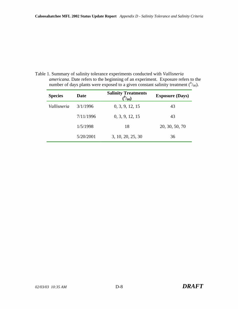
Caloosahatchee MFL 2002 Status Update Report Appendix D - Salinity Tolerance and Salinity Criteria
02/03/03 10:35 AM D-8 DRAFT
Table 1. Summary of salinity tolerance experiments conducted with Vallisneriaamericana. Date refers to the beginning of an experiment. Exposure refers to thenumber of days plants were exposed to a given constant salinity treatment (0/00).
Species Date Salinity Treatments(0/00)
Exposure (Days)
Vallisneria 3/1/1996 0, 3, 9, 12, 15 43
7/11/1996 0, 3, 9, 12, 15 43
1/5/1998 18 20, 30, 50, 70
5/20/2001 3, 10, 20, 25, 30 36

Caloosahatchee MFL 2002 Status Update Report Appendix D - Salinity Tolerance and Salinity Criteria
02/03/03 10:35 AM D-9 DRAFT
Figure D-1. Distribution of Vallisneria americana and Halodule wrightii in theCaloosahatchee Estuary. Also shown are the locations of grass bed monitoring stationsand the general locations of salinity recorders at S-79, Rt. 31 Bridge, Fort Myers Bridges,and Shell Point.

Caloosahatchee MFL 2002 Status Update Report Appendix D - Salinity Tolerance and Salinity Criteria
02/03/03 10:35 AM D-10 DRAFT
Figure D-2. Net exponential growth rates (r + 95% C.I.) of Vallisneria americanameasured in laboratory mesocosms during constant exposure to different salinities. Anegative value of r indicates mortality.
Vallisneria Shoots
Salinity Treatment
0 5 10 15 20 25 30 35
Exp
onen
tial G
row
th r
(pe
r da
y)
-0.20
-0.15
-0.10
-0.05
0.00
0.05
0.10
1/5/19985/20/20013/1/19967/11/1996
Vallisneria Blades
Salinity Treatment
0 5 10 15 20 25 30 35
Exp
onen
tial G
row
th r
(pe
r da
y)
-0.30
-0.25
-0.20
-0.15
-0.10
-0.05
0.00
0.05
0.10

Caloosahatchee MFL 2002 Status Update Report Appendix D - Salinity Tolerance and Salinity Criteria
02/03/03 10:35 AM D-11 DRAFT
Figure D-3. Shoot density of Vallisneria americana at monitoring stations 1, 2, 3 and 4as a function of salinity on the day of collection (top panel) and average discharge at S-79for the 30 days prior to the day of collection (bottom panel).
Vallisneria and Discharge
30-day Average Discharge at S-79 (m3sec-1)
0 25 50 75 100 125 150 175
Sho
ots
/ m2
0
200
400
600
800
1000
1200
1400
Vallisneria and Salinity
Salinity (ppt)
0 5 10 15 20 25 30
Sho
ots/
m2
0
200
400
600
800
1000
1200
1400

Caloosahatchee MFL 2002 Status Update Report Appendix D - Salinity Tolerance and Salinity Criteria
02/03/03 10:35 AM D-12 DRAFT
Salinity 20 ppt
Day of Experiment
0 10 20 30 40 50
Num
ber
of S
hoot
s pe
r T
ub
0
10
20
30
40
50
60
70
80
Mesocosm 3Mesocosm 9
A A
B
C
D DD
Figure D-4. Average number of shoots per tub in two replicate mesocosms exposed to 20 ppt. Letters indicate results of a comparison of daily means using the Student -Newman-Keuls test. Days with different letters are statistically different (p<0.05).

Technical Documentation to Support Development ofMinimum Flows and Levels for the Caloosahatchee
River and Estuary
Appendix E
DRAFT
CERP Projects in the C-43 Basin
Contents
Caloosahatchee River (C-43) Basin Aquifer Storage and Recovery -Pilot Project (2008) ........ E-1Caloosahatchee Back-pumping with Stormwater (2014) Treatment Project............................. E-1C-43 Basin Storage Reservoir Project, Part 1 (2011) .............................................................. E-2C-43 Basin Aquifer Storage and Recovery Project, (2018) Part 2............................................ E-3
South Florida Water Management District
January 2003


Caloosahatchee MFL 2002 Status Update Report Appendix E - CERP Projects in the C-43 Basin
02/03/03 10:37 AM E-1 DRAFT
CERP Projects in the C-43 Basin
Caloosahatchee River (C-43) Basin Aquifer Storage and Recovery -PilotProject (2008)
Project Description: Aquifer Storage and Recovery wells are proposed in order to
maximize the benefits associated with the Caloosahatchee River Storage Reservoir. A
pilot project for these wells is necessary to identify the most suitable sites for the aquifer
storage and recovery wells in the vicinity of the reservoir and to determine the optimum
configuration of those wells. The pilot project will provide information regarding the
characteristics of the aquifer system within the Caloosahatchee River Basin as well as
determine the hydrogeological and geotechnical characteristics of the upper Floridan
Aquifer. The pilot project will also determine the specific water quality characteristics of
waters to be injected, the specific water quality characteristics and the amount of water
recovered from the aquifer, and the water quality characteristics of water within the
receiving aquifer.
Caloosahatchee Back-pumping with Stormwater (2014) Treatment Project
Project Description: This project includes pump stations and a stormwater treatment
area with a total capacity of approximately 20,000 acre-feet located in the C-43 Basin in
Hendry and Glades Counties. The initial design of the stormwater treatment area assumed
5,000 acres with the water level fluctuating up to 4 feet above grade. The final size, depth
and configuration of this facility will be determined through more detailed planning and
design. The purpose of this feature is to capture excess C-43 Basin runoff, which will be
used to augment regional system water supply. Backpumping will only occur after
estuary and agricultural/urban demands have been met in the basin and when water levels
in the C-43 storage reservoir exceed 6.5 feet above grade. Further, Lake Okeechobee
water levels must be within a a specified range to accept this water so as to not impact
ecological resources. When these conditions are met, a series of pump stations will back-
pump excess water from the reservoir and the C-43 Basin to Lake Okeechobee after
treatment through a stormwater treatment area. The stormwater treatment area will be

Caloosahatchee MFL 2002 Status Update Report Appendix E - CERP Projects in the C-43 Basin
02/03/03 10:37 AM E-2 DRAFT
designed to meet Lake Okeechobee phosphorus and other pollutant loading reduction
targets consistent with the Surface Water Improvement and Management Plan for the
Lake and future appropriate pollution load reduction targets which may be developed for
the Lake and the watershed in which the facility is to be located.
C-43 Basin Storage Reservoir Project, Part 1 (2011)
Project Description: This project is the first part of the C-43 Basin Storage Reservoir
and ASR component. The project includes an above ground reservoir with a total storage
capacity of approximately 160,000 acre-feet located in the C-43 Basin in Hendry, Glades,
or Lee Counties. The initial design of the reservoir assumed 20,000 acres with water
levels fluctuating up to 8 feet above grade. The final size, depth and configuration of this
facility will be determined through more detailed planning and design. The purpose of
this project is to capture C-43 Basin runoff and releases from Lake Okeechobee. The
reservoir will be designed for water supply benefits, some flood attenuation, to provide
environmental water supply deliveries to the Caloosahatchee Estuary, and water quality
benefits to reduce salinity and nutrient impacts of runoff to the estuary. It is assumed that,
depending upon the location of the reservoir and pollutant loading conditions in the
watershed, the reservoir could be designed to achieve significant water quality
improvements, consistent with appropriate pollution load reduction targets. Excess runoff
from the C-43 Basin and Lake Okeechobee flood control discharges will be pumped into
the proposed reservoir. Lake Okeechobee will meet any estuarine demands, not met by
basin runoff as long as the lake stage is above a pre-determined level. Lake water will
also be used to meet the remaining basin demands subject to supply-side management.
The C-43 reservoir will also be operated in conjunction with the Caloosahatchee Back-
pumping project, which includes a stormwater treatment area for water quality treatment.
If the level of water in the reservoir exceeds 6.5 feet and Lake Okeechobee is below a
pre-determined level, then water is released and sent to the back-pumping facility.

Caloosahatchee MFL 2002 Status Update Report Appendix E - CERP Projects in the C-43 Basin
02/03/03 10:37 AM E-3 DRAFT
C-43 Basin Aquifer Storage and Recovery Project, (2018) Part 2
Project Description: This project is the second part of the C-43 Basin Storage Reservoir
and ASR component. This project includes aquifer storage and recovery wells with a total
capacity of approximately 220 million gallons per day and associated pre- and post-
water quality treatment located in the C-43 Basin in Hendry, Glades, or Lee Counties.
The initial design of the wells assumed 44 wells, each with the capacity of 5 million
gallons per day with chlorination for pre-treatment and aeration for post-treatment. The
level and extent of treatment and number of the aquifer storage and recovery wells may
be modified based on findings from a proposed aquifer storage and recovery pilot project
(U.S. Environmental Protection Agency, 1999). The purpose of this project is to capture
C-43 Basin runoff and releases from Lake Okeechobee. The wells will be designed for
water supply benefits, some flood attenuation, water quality benefits to reduce salinity
and nutrient impacts of runoff to the estuary, and to provide environmental water supply
deliveries to the Caloosahatchee Estuary. Excess runoff from the C-43 Basin and Lake
Okeechobee flood control discharges will be pumped into the C-43 Basin Reservoir.
Water from the reservoir will be injected into the aquifer storage and recovery wellfield
for long-term (multi-season) storage. Any estuarine demands, not met by basin runoff and
the aquifer storage and recovery wells, will be met by Lake Okeechobee as long as the
lake stage is above a pre-determined level. Lake water is also used to meet the remaining
basin demands subject to supply-side management.

Technical Documentation to Support Development ofMinimum Flows and Levels for the Caloosahatchee
River and Estuary
Appendix F
Hydrodynamic and Salinity Modeling
Chenxia Qiu, Staff Engineer
Contents
Summary ................................................................................................................................ F-1Background ............................................................................................................................ F-1Modeling Approach – CH3D Model & Regression Model ...................................................... F-1
CH3D model....................................................................................................................... F-2Description of the grid ...................................................................................................... F-2Model calibration ............................................................................................................. F-4
Description of the calibration scenario........................................................................... F-4Calibration results ......................................................................................................... F-4
Equilibrium relations between salinity and discharge........................................................ F-8Estimating total estuarine inflow....................................................................................... F-9
Regression model................................................................................................................ F-9The spatial interpolation of salinity at Bird Island and Site 2........................................... F-10Regression model formulae ............................................................................................ F-11Salinity at Bridge 31 station............................................................................................ F-11Regression model calibration results............................................................................... F-12
Assessing CERP: Prediction of salinity for without project (95 base) and with project (2020with Restudy) ................................................................................................................... F-14
Conclusions .......................................................................................................................... F-17References ............................................................................................................................ F-17
Florida Bay and Lower West Coast DivisionSouthern District Restoration Department
South Florida Water Management District
January 2003


Caloosahatchee MFL 2002 Status Update Report Appendix F - Hydrodynamic and Salinity Modeling
02/03/03 10:39 AM F-1 DRAFT
Hydrodynamic and Salinity Modeling
Chenxia Qiu, Staff EngineerSeptember 2002
SummaryThe MFL update utilized CH3D hydrodynamic and salinity model and a regression
model to investigate the salinity distribution in Caloosahatchee River. The Tidal Caloosahatcheebasin model was applied to estimate the ground water and tributary input. The steady statesimulation confirmed the previous MFL rule. Under current conditions, the 300 cfs at S-79 ismatched by an additional 200 cfs or greater of tidal watershed inflow about 50% of the time. Atthe steady state, the combined flow of 500 cfs produces a salinity of about 10 ppt at Ft. Myers.An assessment of the recommended CERP alternative indicated that modified flows would createdesirable salinity levels at Bird Island and Site 2 for the 2020 with Restudy scenario.
BackgroundA Minimum Flow and Level Rule (MFL) for the Caloosahatchee River and Estuary was
adopted in September 2001. Best available information indicted that a mean monthly flow of300 cfs at the Franklin Lock and Dam was required to maintain sufficient salinity to prevent a30-day average salinity concentration exceeding 10 parts per thousand (ppt) at the Ft. Myerssalinity station.
A peer review of the technical documentation supporting the rule endorsed the generalapproach. However, the review panel concluded that the uncertainty in the estimate of theneeded freshwater inflows was too large but this deficiency could be remedied by furtherresearch in key areas. The statistical approach used by the District indicated that 300 cfs wouldmaintain a salinity of about 10 ppt at Ft. Myers. However, the error surrounding this estimatewas large (95% confidence ranged 5.4-17.4 ppt). The panel concluded that the statisticalapproach was flawed and strongly recommended that a mass balance modeling approach be usedin predicting salinity and assessing minimum flows (Edwards et al. 2000). They furthersuggested that a mass balance model of Charlotte Harbor being developed at the University ofFlorida be used to refine the salinity simulations for the Caloosahatchee Estuary once it isavailable (Edwards et al. 2000).
The simulation of Caloosahatchee River MFL update utilized partial deliverables fromthe above project. The Caloosahatchee River portion of the Charlotte Harbor Model was furthercalibrated to derive the relationships between the fresh water discharge and the distribution ofsalinity.
The original technical documentation of the Caloosahatchee MFL concluded that underpresent conditions, the MFL could not be met. The recovery strategy for attaining the MFLrelies on construction projects to be completed by CERP. An additional goal of the modelingeffort was to predict the effect of CERP projects on salinity in the downstream estuary.
Modeling Approach – CH3D Model & Regression ModelThe salinity model for Caloosahatchee River was developed from a CH3D Charlotte
Harbor model (Sheng, 2002), a 3-dimensional fully coupled hydrodynamic and salinity model on

Caloosahatchee MFL 2002 Status Update Report Appendix F - Hydrodynamic and Salinity Modeling
02/03/03 10:39 AM F-2 DRAFT
curvilinear grids. The Charlotte Harbor model was calibrated using data collected during thesummer of 1986 at 6 stations located in Pine Island Sound and around the Peace River inCharlotte Harbor. The hydrodynamic model was calibrated with a 2 months of data, while thesalinity model was calibrated with a 2 weeks of data. The Caloosahatchee and San Carlos Bayportion of the model were not calibrated.
This study calibrated the Caloosahatchee River portion of the model using a 2.5 monthsperiod of data, collected every 15 minutes at five stations. Equilibrium relationships betweenfresh water discharge and salinity in the estuary were derived from a series of steady statesimulations. In turn, a regression model was constructed based on these salinity dischargerelationships. The regression model was calibrated with a 10-year period of salinity records atBridge 31 (BR31) and Ft. Myers, as well as a 6-month record at Bird Island.
CH3D model
The CH3D model is three-dimensional and employs curvilinear grids. The modelsimulates time-dependent circulation in estuaries, lakes, and coastal waters. It solves the three-dimensional equations of motion in a non-orthogonal boundary-fitted coordinate system withgiven computational domain, initial conditions, and boundary conditions. For the presentapplication to the Charlotte Harbor estuarine system, the model solves the conservationequations for the following hydrodynamic variables: surface elevation, 3-D velocities, salinity,and density. The detailed model equations and description can be found in Sheng (1987, 1989,and 2001).
Description of the gridThe computational grid and bathymetry used for the Caloosahatchee River and Charlotte
Harbor estuarine system are shown in Figure F-1. It contains 145 by 225 horizontal cells and 8vertical layers. This grid was generated using a grid generation program originally developed byThompson (1985). The depth information was based on the raw data obtained from theGeophysical Data System of the National Geophysical Data Center. Bathymetry for navigationchannels in San Carlos Bay and the vicinity of Sanibel Causeway were based on the latest dataprovided by Lee County in December 1999. The depths were converted to NAVD88 datumlevel with 12 benchmarks near Charlotte Harbor. The model has intensive grids, extending fromthe north at Charlotte Harbor to the south at Estero Bay. It has eight tributary inflows with fourrivers in Estero Bay, 3 rivers in Charlotte Harbor and 1 river in San Carlos Bay. Total grid isabout 130,000 with horizontal grids 32,000 and 8 vertical layers. The smallest grid cell is about100 to 150 m. The model extends to the Gulf of Mexico eliminating the boundary effects(Figure F-1).
Figure F-2 is the detailed view of Caloosahatchee River portion and the location ofmonitoring stations. The bathymetry was modified based on the cross-section profile data fromScarlatos (1988).

Caloosahatchee MFL 2002 Status Update Report Appendix F - Hydrodynamic and Salinity Modeling
02/03/03 10:39 AM F-3 DRAFT
Figure F-1 Computation grid and bathymetry
Figure F-2. Bathymetry on Caloosahatchee River and location of monitoring stations -- Salinitymonitoring stations: S79, Bridge 31 (BR31), Ft. Myers, Shell Point (Marker H) andSanibel; Seagrass monitoring stations: Bird Island and Site 2.
S79
Ft. Myers
Imperial River
Spring Creek
Estero RiverMuttock Creek
Caloosahatchee River
Shell Creek
Peace RiverMayaka River
Charlotte Harbor
San CarlosBay
Estero Bay
Pine
IslandS
ound
10009008007006005004003002001000
Depth (cm)
S79Bridge 31(BR31)
Ft. Myers
Shell PointMarker H
Sanibel
Bird IslandSite 2
10009008007006005004003002001000
Depth (cm)

Caloosahatchee MFL 2002 Status Update Report Appendix F - Hydrodynamic and Salinity Modeling
02/03/03 10:39 AM F-4 DRAFT
Model calibration
Description of the calibration scenario
The calibration encompassed the dry season period from October 15th to December 31th
2000. The calibration data set was composed of 2 water surface elevation monitoring stationsand 5 salinity stations. The water surface elevation stations are located at Shell Point(maintained by the district), and Ft. Myers (maintained by NOAA). Five (5) salinity monitoringstations are located at S79, Bridge 31 (BR31), Ft. Myers, Shell Point (Marker H), and Sanibel.The tidal boundary condition was derived from Shell Point water surface elevation monitoringdata. The driving forces included freshwater discharge at S-79, tide, wind, rainfall andevaporation.
Calibration results
Figure F-3 shows the calibration of water surface elevation at Shell Point: thedownstream boundary of the Caloosahatchee estuary. The solid line is the model result, and thedotted line is the monitoring data. The modeling results are close to the monitoring data.
Figure F-3 Water surface elevation calibration at Shell Point (Marker H)

Caloosahatchee MFL 2002 Status Update Report Appendix F - Hydrodynamic and Salinity Modeling
02/03/03 10:39 AM F-5 DRAFT
Figure F-4 shows the calibration of water surface elevation at Ft. Myers. This stationdata reflects the tide upstream on the River. The simulated tide range is close to the real data buta little larger than the real data.
Figure F-4 Water surface elevation calibration at Ft. Myers
Figure F-5 presents the salinity calibration results at S79, down stream of the lockstructure, and Bridge 31, located between S79 and Ft. Myers. The thick solid line is thesimulated salinity at the second layer from the water surface (25% of the total depth), while thethin solid line is the simulated salinity at the second layer from the bottom (75% of the totaldepth). The dotted line is the real data at the surface sensor, while the dashed line is the real dataat the bottom sensor. In November, the only discharge event was from the 22nd to 26 th (Juliandays 327-332). So the salinity kept rising until the discharge began.

Caloosahatchee MFL 2002 Status Update Report Appendix F - Hydrodynamic and Salinity Modeling
02/03/03 10:39 AM F-6 DRAFT
Figure F-5 Salinity calibration at S79 and BR31
Figure F-6 shows the simulation results at Ft. Myers, Shell Point and the Sanibel stationin San Carlos Bay. The daily salinity fluctuation range is close to the monitoring data. Themodel results show good agreement with the monitoring data. At the Sanibel station during avery dry period (December 2000), the salinity in the surface layer was higher than in the bottomlayer. The salinity could reach up to 38 ppt. This indicates that evaporation plays a key role inSan Carlos Bay. To solve this problem, accurate evaporation data, along with coincident salinitymonitoring data in San Carlos Bay and Charlotte Harbor will be needed. It will slightly affectthe salinity in the upstream River.
Julian Day
Sal
inity
(ppt
)
300 325 3500
5
10
15
20
25BR31
Julian Day
Sal
inity
(ppt
)
300 325 3500
5
10
15
20
25Simulated surfaceMeasured surfaceSimulated bottomMeasured bottom
S79

Caloosahatchee MFL 2002 Status Update Report Appendix F - Hydrodynamic and Salinity Modeling
02/03/03 10:39 AM F-7 DRAFT
Figure F-6 Salinity calibration at Ft. Myers, Shell Point and Sanibel
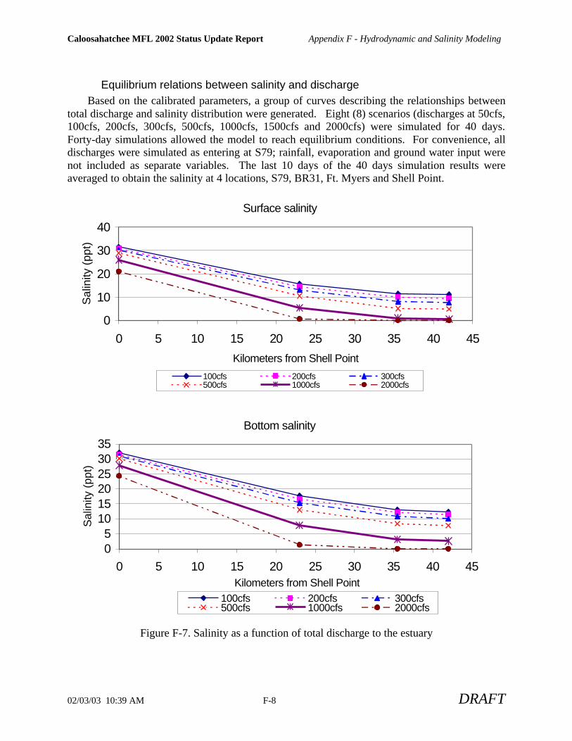
Caloosahatchee MFL 2002 Status Update Report Appendix F - Hydrodynamic and Salinity Modeling
02/03/03 10:39 AM F-8 DRAFT
Equilibrium relations between salinity and dischargeBased on the calibrated parameters, a group of curves describing the relationships between
total discharge and salinity distribution were generated. Eight (8) scenarios (discharges at 50cfs,100cfs, 200cfs, 300cfs, 500cfs, 1000cfs, 1500cfs and 2000cfs) were simulated for 40 days.Forty-day simulations allowed the model to reach equilibrium conditions. For convenience, alldischarges were simulated as entering at S79; rainfall, evaporation and ground water input werenot included as separate variables. The last 10 days of the 40 days simulation results wereaveraged to obtain the salinity at 4 locations, S79, BR31, Ft. Myers and Shell Point.
Figure F-7. Salinity as a function of total discharge to the estuary
Surface salinity
0
10
20
30
40
0 5 10 15 20 25 30 35 40 45
Kilometers from Shell Point
Sal
inity
(pp
t)
100cfs 200cfs 300cfs500cfs 1000cfs 2000cfs
Bottom salinity
05
101520253035
0 5 10 15 20 25 30 35 40 45Kilometers from Shell Point
Sal
inity
(pp
t)
100cfs 200cfs 300cfs500cfs 1000cfs 2000cfs

Caloosahatchee MFL 2002 Status Update Report Appendix F - Hydrodynamic and Salinity Modeling
02/03/03 10:39 AM F-9 DRAFT
Estimating total estuarine inflowThe dominant source of inflow to the Caloosahatchee estuary is runoff from the East and
West Caloosahatchee Drainage Basin – which enters the estuary at the S-79 structure. However,flows from the tidal watershed are also significant. Previous empirical modeling establishedrelationships between flows at S-79 and salinity within the estuary but specific information ontidal Caloosahatchee flows and direct rainfall and evaporation were only included implicitly inthe statistical model through observed salinity data. The hydrodynamic modeling used in thisanalysis requires explicit knowledge of all waters entering estuary.
Unfortunately, few tidal Caloosahatchee inflows are monitored. However, a watershedhydrologic/hydraulic model has been recently been developed for the Tidal CaloosahatcheeWatershed (Peterson, 2002) that can predict tidal inflows. A special simulation of the watershedmodel was conducted to generate daily estuary inflows by source over the length of the estuaryin three years.
Model results were used to develop a characteristic relationship between S-79 flows andtotal inflows. (Details on the hydrologic assessment are discussed in a separate appendix of the2002 MFL report.) S-79 flows dominate under high flow conditions while local tidal inflowsdominate under low flow conditions. Under current conditions, a discharge of 300 cfs at S-79corresponds to a total inflow of 500 cfs or greater about 50% of the time. Under currentconditions, a mean monthly discharge of 300 cfs would be expected to prevent an exceedance ofthe 10 ppt criteria about half of the time.
Regression model
The CERP project in the C-43 basin comprises the recovery strategy for theCaloosahatchee MFL. When completed, these projects should supply the supplemental flowrequired to protect tape grass in the upper estuary.
In the original technical documentation, this proposition was evaluated using two 31 year(1965-1995) estimates of discharge at S-79. These were (1) the common 1995-base case whichassumes 1995 land use and current water management operations in the C-43 basin and (2) afuture base case (2020 with Restudy) which includes predicted 2020 land uses and the majorityof CERP projects in the C-43 basin (reservoirs, aquifer storage and recovery wells (ASR), andback pumping).
Sine the hydrodynamic model cannot be run for 31 years, a regression model wasdeveloped to generate a 31-year record of salinity over Vallisneria beds at 2 stations in the upperestuary. The stations are in the 640-acre area to be protected by the MFL and Vallisneria hasbeen monitored at these sites since 1998. The sites are referred to as Bird Island (upstream) andSite 2 (see Figure F-2).
A regression model was constructed and calibrated at Ft. Myers and Bridge 31 where 15-minute of salinity data were monitored. The salinity at Bird Island and Site 2 (Figure F-2) wereinterpolated with the salinity results from regression model at Ft. Myers and Bridge 31.

Caloosahatchee MFL 2002 Status Update Report Appendix F - Hydrodynamic and Salinity Modeling
02/03/03 10:39 AM F-10 DRAFT
The spatial interpolation of salinity at Bird Island and Site 2Since 1998, the District started seagrass sampling at Bird Island and Site2 monthly.
During each monthly sampling event, salinity was taken from Hydrolab reading. In addition, theDistrict started monitoring salinity data at Bird Island at 15-minute interval since December2001. To get the interpolation parameters at Bird Island and Site 2, 15-minute of salinity data atFt. Myers and Bridge 31 were averaged daily to obtain daily salinity variation. Then, the spatialinterpolation was conducted to fit the monthly sampling data at Bird Island and Site 2, as well asa 6-month daily salinity data at Bird Island. The interpolation results are presented in Figure F-8 and Figure F-9. The interpolated salinity data was used for calibration of seagrass model. Thespatial interpolation formulae are:
At Bird Island, S Bird Island = 0.2* S Ft. Myers + 0.8* S BR31
At Site 2, during salinity increases, S Site 2 = 0.6* S Ft. Myers + 0.4* S Bird Island
during salinity decreases, S Site 2 = 0.4* S Ft. Myers + 0.6* S Bird Island
Figure F-8 Spatial interpolation of measured salinity for Bird Island
Figure F-9 Spatial interpolation of measured salinity for Site 2
05
10152025
Jan-98 Jul-98 Jan-99 Jul-99 Jan-00 Jul-00 Jan-01 Jul-01 Jan-02 Jul-02Date
Sal
inity
(pp
t)
Bird island-daily measured Measured interpolation Bird island monthly data
0
10
20
30
Jan-98 Jul-98 Jan-99 Jul-99 Jan-00 Jul-00 Jan-01 Jul-01 Jan-02 Jul-02Date
Sal
inity
(pp
t)
site 2 monthly data measured interpolation

Caloosahatchee MFL 2002 Status Update Report Appendix F - Hydrodynamic and Salinity Modeling
02/03/03 10:39 AM F-11 DRAFT
Regression model formulaeThe regression model calculated salinity in two steps. Firstly, salinity was calculated
from surface layer equilibrium relations between salinity and discharge derived from the steadystate simulations with CH3D model. Secondly, salinity was further corrected based on theestuary storage effect and tidal flushing. The total discharge was composed of S-79 discharge,and 50% of total basin runoff and the ground water flow to the entire Caloosahatchee River,since 50% of the tidal basin runoff enter into the River at the upstream of Ft. Myers. The groundwater and tributary flow was calculated with rainfall driven formula based on tidalCaloosahatchee hydrology model (Peterson, 2002). Salinity at Ft. Myers station.
At the time step n+1, the salinity at Ft. Myers station (Sn+1) was calculated with the followingformulae .
Sn+1’ = 0 1300cfs < flowSn+1’ = 5E-06*(total flow)2 - 0.0184* total flow + 18.566 50 cfs < flow < 1300 cfsSn+1’ = 35 - (35- 19.5 )* total flow/50cfs 0 < flow < 50 cfsSn+1’ = 35 flow = 0
Figure F-10 Formula for preliminary calculation of salinity at Ft. Myers
To include the estuary flushing effect,
Sn+1 = Sn +( Sn+1’ - Sn)*Ratio_up if Sn+1 > Sn
Sn+1 = Sn +( Sn+1’ - Sn)*Ratio_down if Sn+1 < Sn
Ratio_up=0.05, Ratio_down=0.05 Sn+1 < 10 pptRatio_up =0.03, Ratio_down=0.02 10 ppt < Sn+1 < 15 pptRatio_up =0.07, Ratio_down=0.1 15 ppt < Sn+1 < 20 pptRatio_up =0.02, Ratio_down =0.01 20 ppt < Sn+1 < 25 pptRatio_up =0.012, Ratio_down =0.01 25 ppt < Sn+1 < 30 pptRatio_up =0.001, Ratio_down =0.001 30 ppt < Sn+1
Salinity at Bridge 31 stationAt the time step n+1, the salinity at Bridge 31 station (Sn+1) was calculated with the
following formula.
Sn+1’ = 0 700cfs < flowSn+1’ = 2E-05*(total flow)2 - 0.0297*total flow + 15.223 50 cfs < flow < 1300 cfsSn+1’ = 35 - (35- 15 )* total flow/50cfs 0 < flow < 50 cfsSn+1’ = 35 flow = 0
Formula at Ft. Myers
010203040
0 150 300 450 600 750 9001050
12001350
15001650
18001950
Total discharge (cfs)
Sal
inity
(ppt
)

Caloosahatchee MFL 2002 Status Update Report Appendix F - Hydrodynamic and Salinity Modeling
02/03/03 10:39 AM F-12 DRAFT
Figure F-11 Formula for preliminary calculation of salinity at BR31
To include the inertial effects of storage and flushing,
Sn+1 = Sn +( Sn+1’ - Sn)*Ratio_up if Sn+1 > Sn
Sn+1 = Sn +( Sn+1’ - Sn)*Ratio_down if Sn+1 < Sn
Ratio_up=0.02, Ratio_down=0.03 Sn+1 < 5 pptRatio_up =0.02, Ratio_down=0.1 5 ppt < Sn+1 < 10 pptRatio_up =0.05, Ratio_down=0.01 10 ppt < Sn+1 < 15 pptRatio_up =0.03, Ratio_down =0.015 15 ppt < Sn+1 < 20 pptRatio_up =0.03, Ratio_down =0.03 20 ppt < Sn+1 < 25 pptRatio_up =0.0005, Ratio_down =0.005 25 ppt < Sn+1
If flow > 4500 cfs, Sn+1 = 0
Regression model calibration resultsThe regression model was calibrated with a 10-year period of daily salinity data at Ft.
Myers and BR31. The calibration results are presented in Figures F-12 and F-13.
Figure F-12 Temporal calibration of regression model at BR31
Formula at BR31
010203040
0 150 300 450 600 750 900 1050 1200 1350 1500 1650 1800
Total discharge (cfs)
Sal
inity
(pp
t)
0
5
10
15
20
25
Jan-92 Jan-93 Jan-94 Jan-95 Jan-96 Jan-97 Jan-98 Jan-99 Jan-00 Jan-01 Jan-02Date
Salin
ity (p
pt)
BR31-measured upper layer BR31-regression model
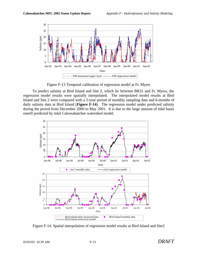
Caloosahatchee MFL 2002 Status Update Report Appendix F - Hydrodynamic and Salinity Modeling
02/03/03 10:39 AM F-13 DRAFT
Figure F-13 Temporal calibration of regression model at Ft. Myers
To predict salinity at Bird Island and Site 2, which lie between BR31 and Ft. Myers, theregression model results were spatially interpolated. The interpolated model results at BirdIsland and Site 2 were compared with a 5-year period of monthly sampling data and 6-months ofdaily salinity data at Bird Island (Figure F-14). The regression model under predicted salinityduring the period from December 2000 to May 2001. It is due to the large amount of tidal basinrunoff predicted by tidal Caloosahatchee watershed model.
Figure F-14. Spatial interpolation of regression model results at Bird Island and Site2
0
5
10
15
20
25
30
Jan-92 Jan-93 Jan-94 Jan-95 Jan-96 Jan-97 Jan-98 Jan-99 Jan-00 Jan-01 Jan-02
Date
Salin
ity (p
pt)
FM-measured upper layer FM-regression model
0
5
10
15
20
25
Jan-98 Jul-98 Jan-99 Jul-99 Jan-00 Jul-00 Jan-01 Jul-01 Jan-02 Jul-02
Date
Salin
ity (p
pt)
Bird island-daily measured data Bird island monthly dataBird Island-regression model
0
5
10
15
20
25
30
Jan-98 Jul-98 Jan-99 Jul-99 Jan-00 Jul-00 Jan-01 Jul-01 Jan-02 Jul-02
Date
Salin
ity (p
pt)
s ite 2 monthly data site2-regression model
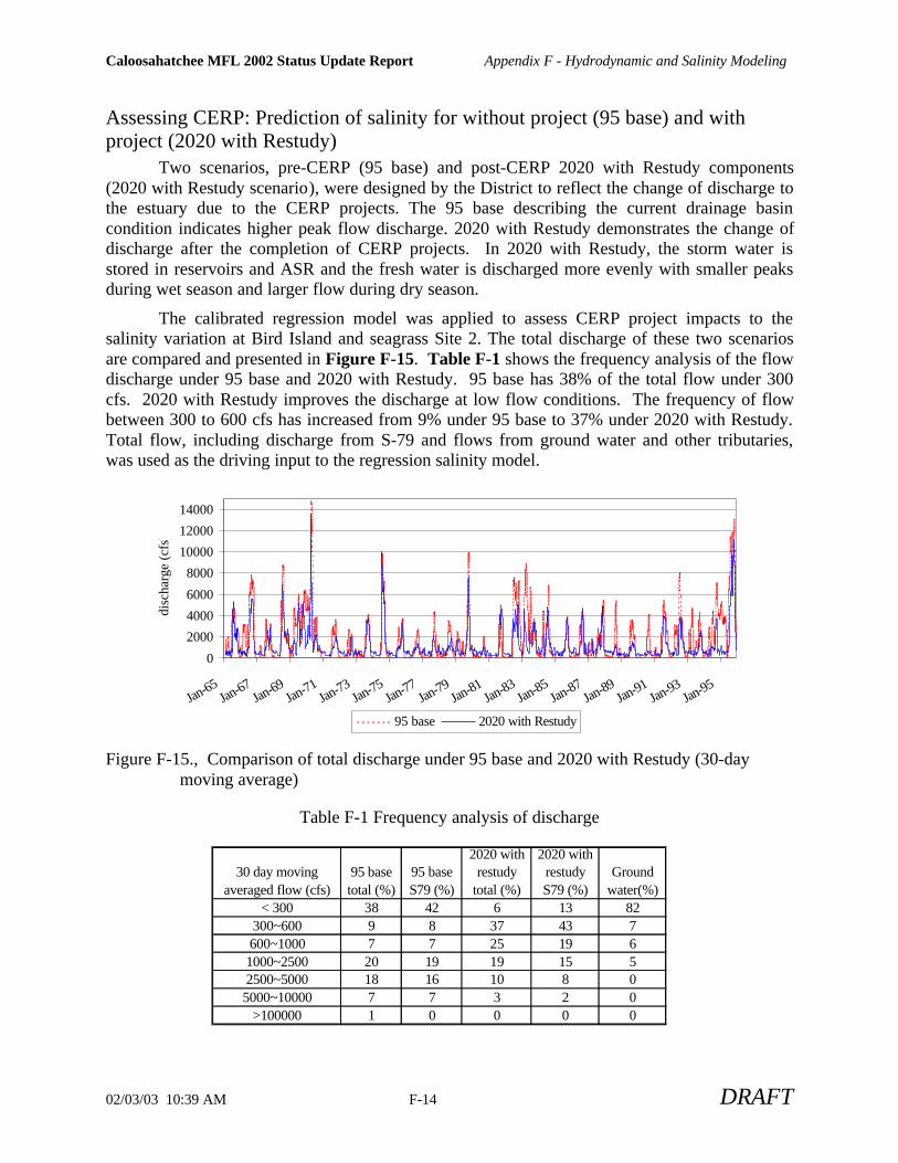
Caloosahatchee MFL 2002 Status Update Report Appendix F - Hydrodynamic and Salinity Modeling
02/03/03 10:39 AM F-14 DRAFT
Assessing CERP: Prediction of salinity for without project (95 base) and withproject (2020 with Restudy)
Two scenarios, pre-CERP (95 base) and post-CERP 2020 with Restudy components(2020 with Restudy scenario), were designed by the District to reflect the change of discharge tothe estuary due to the CERP projects. The 95 base describing the current drainage basincondition indicates higher peak flow discharge. 2020 with Restudy demonstrates the change ofdischarge after the completion of CERP projects. In 2020 with Restudy, the storm water isstored in reservoirs and ASR and the fresh water is discharged more evenly with smaller peaksduring wet season and larger flow during dry season.
The calibrated regression model was applied to assess CERP project impacts to thesalinity variation at Bird Island and seagrass Site 2. The total discharge of these two scenariosare compared and presented in Figure F-15. Table F-1 shows the frequency analysis of the flowdischarge under 95 base and 2020 with Restudy. 95 base has 38% of the total flow under 300cfs. 2020 with Restudy improves the discharge at low flow conditions. The frequency of flowbetween 300 to 600 cfs has increased from 9% under 95 base to 37% under 2020 with Restudy.Total flow, including discharge from S-79 and flows from ground water and other tributaries,was used as the driving input to the regression salinity model.
Figure F-15., Comparison of total discharge under 95 base and 2020 with Restudy (30-daymoving average)
Table F-1 Frequency analysis of discharge
0
2000
4000
6000
8000
10000
12000
14000
Jan-65
Jan-67
Jan-69
Jan-71
Jan-73
Jan-75
Jan-77Jan-79
Jan-81
Jan-83
Jan-85
Jan-87
Jan-89
Jan-91Jan-93
Jan-95
disc
harg
e (c
fs)
95 base 2020 with Restudy
30 day moving averaged flow (cfs)
95 base total (%)
95 base S79 (%)
2020 with restudy
total (%)
2020 with restudy S79 (%)
Ground water(%)
< 300 38 42 6 13 82300~600 9 8 37 43 7600~1000 7 7 25 19 6
1000~2500 20 19 19 15 52500~5000 18 16 10 8 05000~10000 7 7 3 2 0
>100000 1 0 0 0 0

Caloosahatchee MFL 2002 Status Update Report Appendix F - Hydrodynamic and Salinity Modeling
02/03/03 10:39 AM F-15 DRAFT
The predicted salinity variations are presented in Figure F-16 and F-17 at Bird Islandand Site 2 respectively. Both figures show that 2020 with Restudy has lower salinity at the peakthan 95 base.
Table F-2 presents the frequency analysis of daily salinity and 30 day moving averagedsalinity at Bird Island and Site 2. At Bird Island, 27% of the daily salinity under 95 basecondition are over 10 ppt, while under 2020 with Restudy only 2% of the daily salinity values areover 10 ppt. At Site 2, 41% of daily salinity are over 10 ppt for 95 base, compared with 14% ofdaily salinity exceeding 10 ppt under 2020 with Restudy. The results demonstrate that CERPprojects improve salinity in the estuary by lowering high peaks.
Figure F-16 Predicted salinity at Bird Island
Figure F-17 Predicted salinity at Site 2
Table F-2 Frequency analysis of predicted salinity at Bird Island and Site 2
05
101520253035
Jan-65Jan-67
Jan-69Jan-71
Jan-73Jan-75
Jan-77Jan-79
Jan-81Jan-83
Jan-85Jan-87
Jan-89Jan-91
Jan-93Jan-95
salin
ity
(ppt
)
Bird Island - 95 base Bird Isalnd - 2020 with Restudy
0
5
10
15
20
25
30
Jan-65Jan-67
Jan-69Jan-71
Jan-73Jan-75
Jan-77Jan-79
Jan-81Jan-83
Jan-85Jan-87
Jan-89Jan-91
Jan-93Jan-95
salin
ity
(ppt
)
Site2 - 95 base Site2 - 2020 with Restudy
daily (%)
30-day moving average (%)
daily (%)
30-day moving average (%)
daily (%)
30-day moving average (%)
daily (%)
30-day moving average (%)
0~5 49 49 53 53 42 41 33 335~10 23 24 45 46 17 19 53 54
10~13 7 8 1 1 14 13 12 1113~15 3 4 0 0 5 6 1 015~20 11 10 1 1 13 12 1 120~25 4 4 0 0 6 6 0 025~30 2 1 0 0 3 2 0 0
salinity (ppt)
Bird Island Site 295 base 2020 with Restudy 95 base 2020 with Restudy

Caloosahatchee MFL 2002 Status Update Report Appendix F - Hydrodynamic and Salinity Modeling
02/03/03 10:39 AM F-16 DRAFT
Figure F-18 presents the daily salinity and 30 day moving averaged salinity at Ft. Myers. TableF-3 shows the frequency analysis of the daily salinity and 30 day moving averaged salinity at Ft.Myers. The MFL rule states that the daily salinity at Ft. Myers should not exceed 20 ppt, whilethe 30 day moving averaged salinity at Ft. Myers should not exceed 10 ppt. For 2020 withRestudy scenario, 1% of the daily salinity values at Ft. Myers are over 20 ppt (Table 2), and 52%of the 30 day moving averaged salinity values are less than 10 ppt. Of the remainingexceedance, 38% are between 10 ppt and 12 ppt. This range of salinity is linked to low flow(300 to 600 cfs) discharge (Table F-1). The predicted salinity at Ft. Myers marginally meet theassumed MFL rules, considering the uncertainty in the results. The point where meets the 30 dayMFL rule occurs near Site 2 (Table F-1), which is 3 kilometers upstream of Ft. Myers, or 2kilometer from the lower boundary of the protected seagrass area. Of the 31 year period ofsimulation time, the predicted salinity meet the 30 day MFL rule in three entire years, 1970,1983 and 1984 (Figure 18). Due to the lack of groundwater input in CH3D calibration, themodel might predict the salinity higher than the real values. Continuing work will improve themodeling performance.
Figure F-18 Predicted salinity at Ft. Myers
Table F-3 Frequency analysis of predicted salinity at Ft. Myers
0
5
10
15
20
25
30
Jan-65 Jan-67 Jan-69 Jan-71 Jan-73 Jan-75 Jan-77 Jan-79 Jan-81 Jan-83 Jan-85 Jan-87 Jan-89 Jan-91 Jan-93 Jan-95
salin
ity
(ppt
)
Ft. Myers daily under 95 base Ft. Myers 30 day averaged under 95 baseFt. Myers daily under 2020 with Restudy Ft. Myers 30-day averaged un der 2020 with Restudy
daily (%)30 day moving
average (%) daily (%) 30 day moving
average (%)0~5 37.9 36.7 25.3 24.55~10 8.6 12.0 25.1 27.210~13 12.5 11.7 39.1 37.613~15 12.5 10.9 8.3 9.215~20 11.6 13.9 1.3 0.820~25 13.4 11.2 0.9 0.7
Ft. Myers salinity (ppt)
95 base 2020 with Restudy

Caloosahatchee MFL 2002 Status Update Report Appendix F - Hydrodynamic and Salinity Modeling
02/03/03 10:39 AM F-17 DRAFT
ConclusionsThe CH3D hydrodynamic and salinity model and a regression model based on the 3-D
model results were utilized to investigate the salinity distribution in the Caloosahatchee River.The 3-dimensional model was calibrated with a two and half months of data. Then, a series ofconstant discharges from S-79 were simulated with CH3D model to establish the equilibriumrelations between salinity and total flow. A regression model was constructed based on theequilibrium relations. The regression model was further calibrated with a 10-year period of dailysalinity data at Ft. Myers and BR31. The regression model results were spatially interpolated toBird Island and Site 2, and compared with 5-year monthly sampling data. The impacts of theCERP project on salinity variation were evaluated with a regression model based on salinitysimulations in a 31-year period.
Under current conditions, a discharge of 300 cfs at S-79 corresponds to a total inflow of500 cfs or greater about 50% of the time. Under current conditions, a mean monthly dischargeof 300 cfs would be expected to prevent an exceedance of the 10 ppt criteria about half of thetime. The assessment of CERP project indicates reduced peak salinity at Bird Island and Site 2for 2020 with Restudy compared with 95 base.
The MFL update incorporated several projects and modeling efforts. The hydrodynamicand salinity model is one of its components. The tidal Caloosahatchee basin model (MIKESHE)was calibrated by Danish Hydraulic Inc. to provide the ground water and tributary flowinformation to the salinity model. The output of salinity model was used to drive Vallisneriaseagrass model to assess the seagrass growth.
The prediction and simulation of these results are limited with data and approaches. Nofine resolution bathymetry data exists on the Caloosahatchee River portion, except cross-sectionprofile information. The tidal Caloosahatchee basin model providing ground water and tributaryflows needs improvement. 3-d hydrodynamic and salinity model requires further validation withground water information. The regression model is a simple approach to estimate the estuaryflushing and storage factor.
The District is working on several aspects to continue the modeling efforts. Thebathymetry survey on the Caloosahatchee River is underway. A grid editing software tool isunder contract to be used to edit the existing grid. The MFL salinity prediction will be enhancedwith new bathymetry data, the improvement of basin model, and a fast 2-d model with fewergrids to replace the regression model.
ReferencesEdwards, R. E., Lung, W, etc., 2001: Final Review Report, Caloosahatchee Minimum Flow Peer
Review Panel, September 27-29, 2000, South Florida Water Management District, pp30.
Konyha, K., 2002: The significance of tidal runoff on flows to the Caloosahatchee Estuary,Technical Memorandum, South Florida Water Management District.
Peterson, M., 2002 (in review): Tidal Caloosahatchee Basin Model, DHI Water & Environment,Technical report to South Florida Water Management District.
Scarlatos, P. D., 1988: Caloosahatchee Estuary Hydrodynamics, South Florida WaterManagement District, Technical Publication 88-7.

Caloosahatchee MFL 2002 Status Update Report Appendix F - Hydrodynamic and Salinity Modeling
02/03/03 10:39 AM F-18 DRAFT
Sheng, Y. P., 2001: Impact of Caloosahatchee Flow on Circulation & Salinity in CharlotteHarbor, Technical Report for South Florida Water Management District, Civil & CoastalEngineering Department, University of Florida, Gainesville, Florida.
Sheng, Y. P., 2001: Users’ Manual of a Three-Dimensional Circulation Model for CharlotteHarbor Estuarine System, Civil & Coastal Engineering Department, University ofFlorida, Gainesville, Florida.
Sheng, Y. P., 1987: On Modeling Three-Dimensional Estuarine and Marine Hydrodynamics,Three-Dimensional Models of Marine and Estuarine Dynamics (J.C.J. Nihoul and B. M.Jamart, Eds.), Elsevier Oceanorgraphy Series, Elsevier, pp 35-54.
Sheng, Y. P., 1989: Evolution of a Three-Dimensional Curvilinear-Grid Hydrodynamics Modelfor Estuaries, Lakes and Coastal Waters: CH3D, Estuarine and Coastal Modeling (M.L.Spaulding Ed.), ASCE, pp40-49.
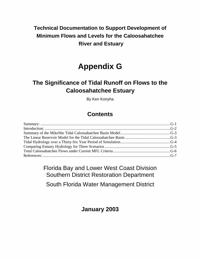
Technical Documentation to Support Development ofMinimum Flows and Levels for the Caloosahatchee
River and Estuary
Appendix G
The Significance of Tidal Runoff on Flows to theCaloosahatchee Estuary
By Ken Konyha
Contents
Summary: ...............................................................................................................................G-1Introduction: ...........................................................................................................................G-2Summary of the MikeShe Tidal Caloosahatchee Basin Model.................................................G-3The Linear Reservoir Model for the Tidal Caloosahatchee Basin ............................................G-3Tidal Hydrology over a Thirty-Six Year Period of Simulation.................................................G-4Comparing Estuary Hydrology for Three Scenarios ................................................................G-5Total Caloosahatchee Flows under Current MFL Criteria ........................................................G-6References: .............................................................................................................................G-7
Florida Bay and Lower West Coast DivisionSouthern District Restoration Department
South Florida Water Management District
January 2003


Caloosahatchee MFL 2002 Status Update Report Appendix G - Significance of Tidal Runoff
02/03/03 10:40 AM G-1 DRAFT
The Significance of Tidal Runoff on Flows to the Caloosahatchee Estuary
Ken Konyha
Summary:
This paper provides the first hydrologic summary of the entire Caloosahatchee Watershed. Until
recently, there was neither measured nor modeled data for the tidal portion of the watershed.
Recently, however, a coupled surface water – groundwater model was developed by DHI for the
Tidal Caloosahatchee. In this paper, an empirical model of the Tidal Caloosahatchee is
calibrated to the DHI model and used to estimate tidal inflows for the extended time-periods
needed for ecological analyses. The estimates of tidal runoff are combined with upstream flows
(estimated by CERP models) to assess the distribution of total inflows to the Caloosahatchee
estuary.
The Tidal Caloosahatchee makes up 30% (268,000 acres) of the watershed area (903,000 acres)
and generates 28% (340,000 acre-feet per year) of the total watershed runoff 1,234,000 acre-feet
per year). Historically, regulatory releases from Lake Okeechobee add an additional 24%
(297,000 acre-feet per year) – mostly at damaging high rates of inflow.
CERP restoration will eliminate most regulatory releases and a substantial amount of non-
beneficial basin runoff will be captured and redirected to beneficial uses: some to agricultural
demands and some to restoring a natural estuarine flow pattern. The flow distribution for total
watershed hydrology is developed for three situations: historic data, the CERP ‘1995 Base’
scenario, and the CERP ‘2020 with Restudy Components’ scenario. The ‘2020 with Restudy’
scenario shows a more natural flow distribution than today’s watershed.
Past work on estuary restoration, including current MFL flow targets, have been based on
conditions in the upstream watershed (S-79 flows). Recent hydrodynamic salinity modeling
shows that total freshwater inflows to the estuary of 500 cfs is more likely to keep salinities
below 10 ppt throughout the Vallisneria seagrass beds. In a comparison of S-79 flows against
total freshwater inflows it was found that, under current conditions (1995 Base), the 300 cfs flow
criterion at S-79 provides and acceptable estimate of 500 cfs total inflows; correlating to total
flows below 500 cfs 43% of the time and to total flows above 500 cfs 57% of the time. The

Caloosahatchee MFL 2002 Status Update Report Appendix G - Significance of Tidal Runoff
02/03/03 10:40 AM G-2 DRAFT
criteria of 300 cfs at S-79 flow will become less acceptable as Restudy components are
constructed. Under the 2020 with Restudy scenario 300 cfs flows at S-79 correlate to total flows
above 500 cfs only 19% of the time.
Introduction:
As part of the Southwest Florida Feasibility Study, DHI Water & Environment was contracted to
develop a hydrologic model of the Tidal Caloosahatchee Watershed. This model, an application
of the MikeShe code, has been completed (Petersen et al, in review). Completion of this model
makes it possible, for the first time, to estimate inflows for the entire Caloosahatchee watershed.
Section 1 presents a brief summary of the Tidal Caloosahatchee model.
The ecology of the estuary is known to depend on freshwater inflows and many problems in the
estuary have been attributed to poor management of these freshwater inflows. The C&SF
Comprehensive Restudy has proposed the construction of several water management facilities to
restore freshwater flows to the estuary.
The objective of this paper is to assess freshwater inflows over a wide variety of climate
conditions using a long (thirty-one year) simulation. Unfortunately, results from Tidal
Caloosahatchee Watershed were only available for three years. Therefore, an application model,
calibrated to the MikeShe model, was created. The application model is based on linear
reservoir theory. Section 2 paper describes the linear reservoir model and compares it to the
MikeShe model. Section 3 applies the model to the entire thirty-one year period of simulation.
In section 4, thirty-one year time-series of Caloosahatchee Estuary inflows are created by
combining Tidal Caloosahatchee runoff with flows from the rest of the watershed (S-79 flows).
Three different sets of estuary flows are created and compared: measured data, the C&SF ‘1995
Base’ scenario, and the ‘C&SF 2020 with Restudy Components’ scenario. Measured data show
historic conditions; ‘1995 Base’ shows conditions as they exist today in the watershed; ‘2020
with Restudy Components’ shows conditions in 2020 after the proposed water management
facilities are constructed.

Caloosahatchee MFL 2002 Status Update Report Appendix G - Significance of Tidal Runoff
02/03/03 10:40 AM G-3 DRAFT
Section 5 uses the ‘1995 Base’ and ‘2020 with Restudy Components’ hydrology to examine the
suitability of the current MFL flow criterion of 300 cfs at S-79.
Summary of the MikeShe Tidal Caloosahatchee Basin Model
The Tidal Caloosahatchee Basin Model (Petersen et al, in review) is an application of the
MikeShe code. The model is a fully coupled surface water and groundwater model intended to
accurately simulate all significant hydrologic process in the watershed including evaporation,
runoff, stormwater detention, river hydraulics, stream water management, groundwater
withdrawals and recharge, etc.
The area modeled is shown in Figure G-1. Table G-1 shows the areas of the drainage basins
within the study area that drain into the Caloosahatchee. The Tidal Caloosahatchee watershed is
268,000 acres (30%), compared to the portion of the non-tidal portion of the Caloosahatchee,
which is 634,000 acres.
The consultant was requested to make a special simulation examining the spatial distribution of
inflows into the estuary and describing inflow sources (Petersen and Copp, 2002). The MikeShe
runoff time-series is shown on Figure G-2. Although measured stream flow data in the basin are
sparse, DHI calibrated to all available data: flows, groundwater elevation data and stream stage
data. For the purposes of this paper, the MikeShe flow data are assumed to be accurate.
The spatial distribution of flows entering the estuary are shown in Figure G-3 and tabulated in
Table G-2. The largest single inflow (30% of the total) comes from Orange River (river
segment 3: six miles downstream of S-79). Substantial volumes (17%) enter far downstream
(segment 10: twenty-six miles downstream of S-79). This spatial distribution was relatively
constant over the simulation period.
The Linear Reservoir Model for the Tidal Caloosahatchee Basin
A linear reservoir (LinRes) model was developed for the Tidal basin because MikeShe results
were only available for a three-year simulation period while flows are needed for a thirty-one
year period of simulation. The Linear Reservoir Model was developed because it is fast, reliable,
and easily calibrated against the MikeShe model.

Caloosahatchee MFL 2002 Status Update Report Appendix G - Significance of Tidal Runoff
02/03/03 10:40 AM G-4 DRAFT
The model has three cascading reservoirs and a root zone. Rainfall and evaporation fill and
empty the root zone with excess root zone water recharging the storage zones (linear reservoirs).
The storage zones drain at a rate exponential to storage. There is also a term for rain falling
directly on the streams and estuary. The equations are:
Root Zone:potential change = max(0, Rain – PET + root zone storage)root zone storage = min(max(0,( potential change)),root zone capacity)actual ET = PET - max(0,-( potential change))water to add to zone 1= max(0, potential change - root storage capacity)
For Each Zone:addwater : excess water defined in previous zonestorage = min(max(0,( addwater + storage –outflow)),maximum capacity)ouflow = (storage) *(1-exp(-1/ storage coefficient))addwater for next zone = max(0,( addwater + storage –outflow)) - maximum capacity
[Fluxes are measured in inches per day and are converted to acre-feet per day by multiplying by
the watershed area.]
The LinRes model was calibrated to MikeShe results, using the same rainfall and PET data.
Since MikeShe simulates three flow types: aquifer flow (AQ), shallow drainage flow (DR) and
overland flow (OVL), the conceptual reservoirs of LinRes were calibrated to match each
MikeShe flow type. Time-series for each flow type (not shown here) were developed; the
average annual flow for each type is shown on Table G-4. [Note: Reservoir 1 simulates AQ
flow, Reservoirs 2 and 3 simulate DR flow, OVL flow is simulated best using the direct rainfall.]
Table G-3 shows the calibrated model parameters.
The final model matched the MikeShe model well and had a Pearson correlation coefficient of
0.878. Figure 2 shows the time-series for both the MikeShe and the LinRes model over the
three-year simulation.
Tidal Hydrology over a Thirty-Six Year Period of Simulation
The calibrated LinRes model was used to generate a thirty-six year (1965-2000) time-series of
tidal watershed runoff. Rainfall and PET data came from Ft Myers (prepared for regional
modeling efforts). A general summary of the hydrology is shown in Table G-4. Note the
variability of rainfall and runoff. The three-year calibration period averaged 65.1 inches per year

Caloosahatchee MFL 2002 Status Update Report Appendix G - Significance of Tidal Runoff
02/03/03 10:40 AM G-5 DRAFT
of rain and 26.1 inches per year of runoff (584,000 acre-foot per year) while the thirty-six
simulation period had only 56.2 inches per year of rainfall and 16.2 inches per year of runoff
(362,000 acre-feet per year). Slow draining aquifer flow (AQ) makes up 23% (84,000 acre-feet
per year) of the total. Aquifer drainage is about the same magnitude as the rainfall that falls
directly onto the open-water of estuary (90,000 acre-foot per year).
Figure 4 shows daily tidal basin runoff for the thirty-one year simulation period (1965-1995).
This simulation period matches the CERP simulation period. Local basin runoff averages
340,000 acre-foot per year and peak daily runoff rates regularly exceed 5000 cfs.
Comparing Estuary Hydrology for Three Scenarios
Salinities in the Caloosahatchee Estuary depend on total estuary inflow. Flows from the tidal
basin (above) are combined with flows from the rest of the watershed to generate time-series of
total estuary inflows. The Caloosahatchee Estuary receives distributed flows from the Tidal
Watershed and a very large point source at the S-79 structure (aka Franklin Lock and Dam) at
the downstream end of the C-43 canal. Flows at S-79 are generated within the upstream
watershed: i.e. the East Caloosahatchee Basin, the West Caloosahatchee Basin, and the S-4
Basin; S-79 flows also include occasional but substantial (and damaging) regulatory releases
from Lake Okeechobee that pass through the C-43 canal into the estuary.
Three time-series for S-79 flows are combined with tidal basin flows and examined: measured S-
79 data, 1995 Base, and 2020 with Restudy Components. ‘Measured’ data represent the historic
watershed; ‘1995 Base’ data represents the current conditions; ‘2020 with Restudy Components’
represents the proposed CERP solution. [One of the CERP objectives is to restore conditions
within the Caloosahatchee Estuary via reservoirs, STAs, etc. The ‘2020 with Restudy
Components’ models the ‘yellow book’ components. (These components are being refined as
part of the C-43 PIR process. No refined hydrology is yet available.)]
Figure G-5 shows the time-series for total freshwater inflows to the estuary for the ‘1995 Base’
and ‘2020 with Restudy Components’ scenarios. Notice the variability in both time-series;
several years in a row without large runoffs and also several years with many large runoffs in the
same year. This variability is rain-driven and natural. Also notice the difference between the

Caloosahatchee MFL 2002 Status Update Report Appendix G - Significance of Tidal Runoff
02/03/03 10:40 AM G-6 DRAFT
two time-series. The ‘2020 with Restudy Components’ has raised the baseflow components and
reduced peak flows.
Figure G-6 shows the probability flow-distribution of freshwater inflows for ‘1995Base’ and
‘2020 with Restudy Components’ scenarios. The same data is shown in tabular form in Table
G-6. The frequency analysis shows that today’s estuary is frequently exposed to low flows.
[These result in high salinities that stress the Vallisneria sea-grasses. Recent hydrodynamic-
salinity modeling has found that total freshwater inflows of 500 cfs are needed to keep salinities
below 10 ppt throughout the productive Vallisneria sea-grass beds. (Qiu, personal
communications).]
Under 1995 Base 41% of the months have flows below the 500 cfs threshold needed to protect
the seagrass beds. Severe stress is also common with 32% of all months having flows below 325
cfs. Flows are much better for the ‘2020 with Restudy Components’ scenario. Only 18% of the
months have flows below the 500 cfs threshold and severe stress is almost eliminated with only
2% of months having flows below 325 cfs.
Total Caloosahatchee Flows under Current MFL Criteria
Existing minimum flow criteria are 300 cfs at S-79. These criteria were established without
quantitative consideration of inflows from the unmonitored tributaries and groundwater inflows
of the tidal basin. Now that hydrology is available for the entire watershed, this minimum flow
value can be reassessed.
Hydrodynamic modeling shows that a combined flow of 500 cfs is necessary to keep salinities
below 10 ppt throughout the critical seagrass beds. The combined watershed hydrology can be
examined under current MFL conditions (300 cfs) to determine how well the MFL flow
correlates to the target watershed flow of 500 cfs.
Table 7 looks at monthly watershed inflows, for all scenarios, when monthly S-79 flows are near
300 cfs (275 to 325 cfs). The frequency analysis of 1995 Base shows that 300 cfs at S-79
correlates reasonably well to the 500 cfs total flow target. When S-79 flows are near 300 cfs,

Caloosahatchee MFL 2002 Status Update Report Appendix G - Significance of Tidal Runoff
02/03/03 10:40 AM G-7 DRAFT
total flows are between 325 cfs and 500 cfs about half of the time (43%) and between 500 cfs
and 800 cfs about half of the time (43%).
The correlation of S-79 flows of 300 cfs and total flows of 500 cfs breaks down under the ‘2020
with Restudy Components’ scenario. Under this scenario, when S-79 flows are near 300 cfs,
total flows are below 500 cfs most of the time (80%) and between 500 cfs and 800 cfs only 20%
of the time.
It is not surprising that the correlation of S-79 flows and total flows changes in the 2020
scenario; reservoirs and ASRs upstream of S-79 are designed to deliver base flows to the estuary.
This shifting of sources is demonstrated in Figure 7. Figure 7 shows the contribution of upper
basin flow as a percentage of total estuary inflow for both 1995 base and 2020 with Restudy
scenarios. Under 1995 Base, upper basins contribute 42% of flows in the 325 cfs - 500 cfs range
and 62% of flows in the 500 cfs – 800 cfs range. Under 2020 with Restudy, upper basins
contribute 78% of flows in the 325 cfs - 500 cfs range and 70% of flows in the 500 cfs – 800 cfs
range.
In summary, it would be better to base protection criteria on total estuary inflows (500 cfs) than
on S-79 flows (300 cfs). Under current conditions (1995 Base), the 300 cfs flow criterion at S-
79 is an acceptable surrogate for total estuary inflows of 500 cfs; correlating to total flows below
500 cfs 43% of the time and to total flows above 500 cfs 57% of the time. The criteria of 300 cfs
at S-79 flow will become less acceptable as Restudy components are constructed. Under the
2020 with Restudy scenario 300 cfs flows at S-79 correlate to total flows above 500 cfs only
19% of the time.
References:
Tidal Caloosahatchee Basin Model - Model Calibration and Validation, Michael J. Petersen,Joseph D. Hughes, Jeremy McBryan, Roger Copp and Torsten V. Jacobsen, DHI Water& Environment, Project 51189, July 2002
Summary Descriptions of Groundwater and Tributary Flows to the Caloosahatchee River.Michael J. Petersen, and Roger Copp, DHI Water & Environment, Project 51189, August22 2002

Caloosahatchee MFL 2002 Status Update Report Appendix G - Significance of Tidal Runoff
02/03/03 10:40 AM G-8 DRAFT
Table G-1. SFWMD Drainage Basins in Caloosahatchee WatershedAcres Mi2
Basins draining directly into Tidal Caloosahatchee EstuaryTidal Caloosahatchee Basin 196,140 306Telegraph Basin 56,474 88Caloosahatchee Estuary 15,376 24
SUB-TOTAL 267,990 418Basins draining into Estuary at S-79East Caloosahatchee Basin 226,631 354West Caloosahatchee Basin 356,928 558S4 Drainage Basin 50,269 79
SUB-TOTAL 633,828 990TOTAL 901,818 1409
Table 2. Spatial Distribution of Tidal Caloosahatchee Inflows (MikeShe estimates)
River Segment Station (MilesDownstream of S-79)
Fraction of FlowEntering at each Station
1 0.44 9%2 5.09 7%3 7.13 29%4 8.16 3%5 9.09 8%6 11.69 5%7 15.11 7%8 18.66 7%9 21.84 8%
10 25.93 17%
Table 3. Parameters of Linear Reservoir Model of Tidal Caloosahatchee BasinArea of Basin 267,990 acresRainfall 1965-2000 measured data (Thiessen polygon average of 10 stations)Evapotranspiration 1965-2000 pseudo-Penman data for Fort MeyersRoot Zone 6.85 inchesDirect Flow 100% of rainfall over 19,207 acres
Maximum Storage (in) Storage Coeff (in/d)Rapid Flow 5 8Moderate Flow 1 100Linear Reservoirs
Slow Flow 2.6 110Pearson GOF vMikeShe Results R = 0.878
Caloosahatchee MFL 2002 Status Update Report Appendix G - Significance of Tidal Runoff
02/03/03 10:40 AM G-9 DRAFT
Table 4. Comparing Tidal Caloosahatchee ModelsRunoff (acre-foot per year)
Model p.o.s.Rainfall(inchesper year)
Runoff(inchesper year) Total AQ DR OVL
MikeShe 1998-2000 65.1 26.1 583,298 104,949 373,531 104,819LinRes 1998-2000 65.1 26.1 584,092 119,630 360,421 104,042LinRes 1965-2000 56.2 16.2 362,488 83,856 188,605 89,927
Table 5. Annual Flows into the Caloosahatchee Estuary: 1965-1995Measured 1995 Base 2020 with Restudy
Average Annual Flow (af/year)Tidal Caloosahatchee Basins 339,471 (22%) 339,471 (24%) 339,471 (32%)S-79 Flow 1,190,097 (78%) 1,070,637 (76%) 717,705 (68%)
E & W Caloos Basins 893,387 (58%) 703,322 (50%) 689,217 (65%)Regulatory Releases 296,710 (19%) 367,314 (26%) 28,488 (3%)
TOTAL 1,529,568 1,410,108 1,057,176note: 1995 Base is from Regional Modeling (95BSRR)note: '2020 with Restudy Components' is from Regional Modeling (2020R1)
Table 6. Frequency Distribution of Total Estuary Inflows (see also Figure 5).Probability of Monthly Flows within Flow Range
Flow Range measured 1995 Base 2020 with Restudy Components<325 cfs 23% 32% 2%
325 to 500 cfs 9% 9% 16%500 to 800 cfs 12% 6% 32%800 to 1500 cfs 13% 12% 25%1500 to 2800 cfs 17% 13% 10%2800 to 4500 cfs 11% 14% 9%4500 to 8000 cfs 11% 9% 4%
>8000 cfs 4% 4% 1%
Table 7. Evaluating watershed inflows when S-79 monthly flows are near 300 cfs (275 to 325 cfs)
probability total flow in range (cfs)Total Flow measured 95base 2020 with Restudy Components
<325 cfs 7% 0% 13%325 to 500 cfs 53% 43% 68%500 to 800 cfs 33% 43% 20%800 to 1500 cfs 7% 14% 0%1500 to 2800 cfs 0% 0% 0%2800 to 4500 cfs 0% 0% 0%4500 to 8000 cfs 0% 0% 0%
>8000 cfs 0% 0% 0%months is in range 15 14 40

Caloosahatchee MFL 2002 Status Update Report Appendix G - Significance of Tidal Runoff
02/03/03 10:40 AM G-10 DRAFT
Figure G-1 – Segments of the Caloosahatchee River Estuary Receiving Inflows from the TidalCaloosahatchee River Watershed
S-79
Ft Myers
Shell Point
Cape Coral

Caloosahatchee MFL 2002 Status Update Report Appendix G - Significance of Tidal Runoff
02/03/03 10:40 AM G-11 DRAFT
Figure G-2. Comparison of 5-day flows: MikeShe Model for the Tidal Caloosahatchee Basin and Calibrated Linear Reservoir Model.
Flows in the Tidal Caloosahatchee:Developing rainfall-driven flows based on MIKESHE flows
-2,000
0
2,000
4,000
6,000
8,000
10,000
12,000
14,000
16,000
18,000
6/19/97 1/5/98 7/24/98 2/9/99 8/28/99 3/15/00 10/1/00 4/19/01
Flo
w (
acre
-fee
t p
er d
ay)
Linear Reservoir Model Flows
MIKESHE flows

Caloosahatchee MFL 2002 Status Update Report Appendix G - Significance of Tidal Runoff
02/03/03 10:40 AM G-12 DRAFT
Figure G-3. Typical Spatial Distribution of Tidal Caloosahatchee Inflows
Figure G-4. Tidal Caloosahatchee Daily Flows predicted by LinRes model
Where Tidal Caloosahatchee Flows enter Estuary
0%
10%
20%
30%
40%
50%
60%
0 5 10 15 20 25 30Location (miles downstream of S-79)
Fra
ctio
n o
f F
low
(%
)
0%
20%
40%
60%
80%
100%
120%
Cu
mu
lativ
e F
low
(%
)
Inflow for SegmentCumulative Inflow
Tidal Caloosahatchee Inflows - LinRes Model Predictions
-1,000
0
1,000
2,000
3,000
4,000
5,000
6,000
7,000
8,000
9,000
1/1/65 6/24/70 12/15/75 6/6/81 11/27/86 5/19/92 11/9/97
date
flo
w (c
fs)
LinResMikeShe

Caloosahatchee MFL 2002 Status Update Report Appendix G - Significance of Tidal Runoff
02/03/03 10:40 AM G-13 DRAFT
Figure G-5. Average Monthly Caloosahatchee Estuary Inflows: modelled S-79 flow for 1995Base and 2020 with ReStudy - each combined with LinRes estimates of tidal flow.
Total Estuary Flow:Modelled S-79 flow plus modelled tidal flow
0
2,000
4,000
6,000
8,000
10,000
12,000
14,000
16,000
J-65 J-67 J-69 J-71 J-73 J-75 J-77 J-79 J-81 J-83 J-85 J-87 J-89 J-91 J-93 J-95
aver
age
mo
nth
ly fl
ow
(cfs
)
1995 Base
2020 with Restudy Components

Caloosahatchee MFL 2002 Status Update Report Appendix G - Significance of Tidal Runoff
02/03/03 10:40 AM G-14 DRAFT
Figure G-6. Distribution of Average Monthly Caloosahatchee Estuary Inflows – 1965 to 1995.Inflows include Upper Basins, Tidal Basin, and Lake Okeechobee regulatory releases.
Figure G-7. Percentage of Average Monthly Caloosahatchee Estuary Inflows contributed byUpper Basins.
0%
10%
20%
30%
40%
50%
60%
70%
80%
90%
100%
<325
cfs
325 t
o 500
cfs
500 t
o 800
cfs
800 t
o 150
0 cfs
1500
to 28
00 cf
s
2800
to 45
00 cf
s
4500
to 80
00 cf
s
>800
0 cfs
1995 Base2020 with Restudy
0%
5%
10%
15%
20%
25%
30%
35%
<325
cfs
325 t
o 500
cfs
500 t
o 800
cfs
800 t
o 150
0 cfs
1500
to 28
00 cf
s
2800
to 45
00 cf
s
4500
to 80
00 cf
s
>800
0 cfs
Fre
qu
ency
of
Occ
urr
ence
1995 base2020 with Restudy

Technical Documentation to Support Development ofMinimum Flows and Levels for the Caloosahatchee
River and Estuary
Appendix H
Development of an Ecological Model to PredictVallisneria americana Michx. Densities in the Upper
Caloosahatchee Estuary: MFL UpdateMelody Hunt
Contents
Summary ................................................................................................................................H-1Background ............................................................................................................................H-1Model Description ..................................................................................................................H-2
State Variable Equations .....................................................................................................H-3Model Calibration...................................................................................................................H-9Assumptions and Limitations: Calibration.............................................................................H-15Sensitivity Analysis ..............................................................................................................H-16
Input Data .........................................................................................................................H-16Parameters ........................................................................................................................H-17Sensitivity Analysis Discussion.........................................................................................H-17
31-Year Scenarios.................................................................................................................H-24Data Needs........................................................................................................................H-24Assumptions and Limitations: 31-Year Scenarios..............................................................H-27
Future Improvements ............................................................................................................H-30Data analysis .....................................................................................................................H-30Model Development..........................................................................................................H-31Experimental /Site Work...................................................................................................H-31
References ............................................................................................................................H-33
Florida Bay and Lower West Coast DivisionSouthern District Restoration Department
South Florida Water Management District
January 2003


Caloosahatchee MFL 2002 Status Update Report Appendix H -- Ecological Model
02/06/03 7:18 PM H-1 DRAFT
Development of an Ecological Model to Predict Vallisneria Americana Michx.Densities in the Upper Caloosahatchee Estuary -- MFL Update
Summary
The density of Vallisneria americana Michx. is estimated using a numerical model developed for
the upper Caloosahatchee Estuary. The density is estimated based on responses to light, salinity
and temperature at two sites within the upper estuary. Monthly field monitoring of V. americana
density and water quality parameters has been conducted at these sites since 1998. The model is
calibrated based on measured V. americana densities, water temperature, and transparency at
each station for the period 1998-2001. Daily salinity input is estimated from flows generated by
hydrodynamic modeling. Daily incident PAR was obtained from a continuous recording station
in Estero Bay. Long–term computations for V. americana are developed using predicted salinity
regimes from both the 95 base scenario (Pre-CERP) and the D13R (Post-CERP) scenario.
Background
V. americana Michx. in the upstream fresh and brackish water portion of the Caloosahatchee
Estuary has been identified in the “Technical Documentation to Support Development of
Minimum Flows and Levels for the Caloosahatchee River and Estuary” (SFWMD, 9/00 Draft) as
a key species to be protected against significant harm. The proposed approach for determining
the minimum flows and levels (MFLs) described in this document included the development of
daily growth rate algorithms for V. americana relating changes in shoot density with salinity.
Because the growth model presented was not intended to reproduce the annual cycle of V.
americana growth or abundance, the shoot density was “reset” each year to a specified constant
value. Additionally, salinity was the only environmental variable considered in this V.
americana growth model. While a scientific review panel endorsed the approach of utilizing V.
americana as an environmental indicator to establish MFLs, they identified areas where further
work was required to validate the MFL. In their final review report, the scientific panel stated
that the “V. americana approach should be refined, improved and made more robust” (Edwards
et al., 2000). The primary criticisms stated by the review panel in the proposed V. americana
model included:

Caloosahatchee MFL 2002 Status Update Report Appendix H -- Ecological Model
02/06/03 7:18 PM H-2 DRAFT
1. using salinity as the global limiting factor to V. americana survival and growth,
2. the lack of variability in spatial and demographic factors,
3. the lack of variability in salinity input regimes,
4. setting annual shoot recovery densities to constant values.
Specifically the review panel recommended that an energetically based V. americana model be
developed to allow prediction of the complete annual cycle of growth, reproduction, senescence,
and overwintering with consideration for multiple environmental factors. Additionally, it was
recommended that a hydrodynamic model be utilized to provide salinity input to the V.
americana model thus permitting the evaluation of a wide range of salinity regimes on SAV
growth and survival.
Model Description
A mechanistic, process based ecological model has been developed to investigate growth
responses of V. americana to varying environmental conditions in the upper Caloosahatchee
Estuary. Due to the limited amount of time available for development and calibration, the model
presented here is in the preliminary stages of development and future modifications are
anticipated. The model consists of a system of 3 simultaneous differential equations (finite
difference), one for each of three state variables, solved by Euler numerical integration with a
time step of 1 day. State variables represented in the model are the following: total mass,
number of shoots and number of blades. The domain of the model is a spatially averaged 1m2
single layer water column. Forcing functions are water temperature, incident PAR, secci disk
depth, and salinity. The water column is modeled as a non-stratified, homogeneous layer. A
conceptual model (Figure H-1) illustrates the core processes that control plant growth and
abundance in the model.

Caloosahatchee MFL 2002 Status Update Report Appendix H -- Ecological Model
02/06/03 7:18 PM H-3 DRAFT
Figure H-1. Conceptual V. americana Model for the Upper Caloosahatchee Estuary
State Variable Equations
The equations for mass (g dry weight Carbon/m2), blade (number of blades/m2) and shoot
density (number of shoots/m2) were all formulated similarly for each of the state variables. The
equation is parameterized for each state variable and repeated three times in the model. The
discussion herein shows the equations for blade density. The basic equations are the same for
the remaining state variables with a simple substitution of these variables. The equation
representing blade density is:
Blade Density (t) = Blade Density (t-dt) + Productivity – Loss
Where:
Productivity = f (Blade Density, Salinity, Temperature, Light)
and
Loss = f (Senescence, Stress Mortality, Respiration)
PAR
Salinity
Temp.
SecciDisk
Primary Inputs &Forcing Functions
Interactions and State Variables
Light Attenuation
SAVPhotosynthesis
LightSaturation
Min.Max.
Optimum
Depth
NumberBlades
NumberShoots
BladeL&W
MORPHOLOGYBIOMASS
Respiration
Leaf Turnover

Caloosahatchee MFL 2002 Status Update Report Appendix H -- Ecological Model
02/06/03 7:18 PM H-4 DRAFT
Loss
Senescence is considered seasonal and is triggered by day and temperature cues, which are based
on both observations in the Caloosahatchee Estuary and the four-year calibration data set. Losses
from respiration and stress mortality are temperature dependent and have the following form:
(Stress Mortality Coefficients * Respiration Coefficient) * (Blade Density2) *
[0.63*exp(0.092*water temperature)].
Stress mortality terms include a separate coefficient for light and salinity. They are utilized only
when conditions fall below tolerance levels for light or salinity. The cues for these coefficients
are currently based on the calibration data set. It is anticipated that this algorithm will be refined
with the quantification of these stresses from a recent mesocosm experiment (Hunt et al., 2002).
If conditions are not outside the tolerance levels, only the base-line respiration coefficient is used
in the calculation.
Productivity
Maximum productivity is multiplied by a series of reduction factors that range from 0-1, with 1
representing productivity at optimal environmental conditions and 0 representing conditions that
prevent productivity. The reduction factors include the effects of salinity, light, and temperature.
Maximum productivity is a density – dependent, self-limitation term determined by calibration
that represents the carrying capacity of the environment. Relative growth effect relationships for
salinity, light and temperature were developed based on field data, experimental studies using V.
americana obtained from the Upper Caloosahatchee Estuary, and from information reported in
the literature (Table H-1).
Table H-1: Summary of Productivity Variables
VARIABLE INPUT DATA RELATIONSHIP PARAMETERS REQUIRED SOURCE
Salinity Salinity, Water-Temperature Graphical
Growth rate at different salinities fortwo different temperature ranges(corresponding to wet /dry seasons)
Doering et al., 1999
LightIncident PARSecci Disk DepthWater Depth
P/I curve Ik = 200 µE/m2*sHarley and Findlay,1994: ReportedRange 100-279
Temperature Water-Temperature
Empirical equation(O’Neill et al.,1972)
Q10 = 2Optimum Temp. = 33 oCMaximum Temp.= 50 oC
Wilkinson, 1963

Caloosahatchee MFL 2002 Status Update Report Appendix H -- Ecological Model
02/06/03 7:18 PM H-5 DRAFT
Salinity Effect
V. americana is a salt-tolerant freshwater species that often occurs in the fresh, oligohaline and
mesohaline reaches of estuaries in the Northeastern and Southeastern United States (Bourn,
1932; Lowden, 1982). Salinity is an important environmental variable regulating the growth
and distribution of V. americana in the upper Caloosahatchee Estuary (Doering et al., 1999).
Relationships were developed relating relative growth to salinity in the range of 0 to 15 based on
mesocosm studies using V. americana obtained from the Caloosahatchee Estuary (Doering et al.,
1999). These researchers report two different rates based on wet season or dry season
experiments. A combined salinity effect was developed in the model for shoots and blades based
on these data and differentiated in the model according to incubation temperatures (Figure H-2).
If the water temperature is > 25 oC then the salinity effect formulated for the wet season is used
and if the water temperature is < 25 oC then the salinity effect formulated for the dry season is
used.
Light Effect
The central role of light availability for submerged aquatic vegetation (SAV) has been
demonstrated in numerous, field, laboratory, and modeling studies. Changes in water clarity can
impact density, depth distribution and species able to grow in a given area. V. americana is
generally considered light adaptable as it acclimates rapidly to increasing light and efficiently
uses low light (Titus and Adams, 1979; Meyers et al., 1943; Harley and Findlay, 1994)
However, its limited elongation potential may be a disadvantage in deep turbid water (Barko et
al., 1984; 1991) and water clarity may an important factor regulating growth and survival
especially for seedlings or immature rosettes (Kimber et al. 1995).
The light available for photosynthesis is modeled based on a simple linear photosynthetic versus
irradiance (P/I) relationship (Blackman, 1905). In the models present formulation, the amount
light reaching the bottom at any given location is assumed to be the amount of light available for
photosynthesis. It is recognized that this is a conservative formulation most appropriate for
small immature plants and likely underestimates the amount available for mature established
plants with leaves extending into the water column.

Caloosahatchee MFL 2002 Status Update Report Appendix H -- Ecological Model
02/06/03 7:18 PM H-6 DRAFT
Figure H-2: Combined Salinity Effect for Shoots and Blades.
Net Blade Growth RateWet Season (>25 C)
0
0.2
0.4
0.6
0.8
1
0 3 6 9 12 15
Salinity
Rel
ativ
e G
row
th R
ateNet Shoot Growth Rate
Wet Season (>25 C)
0
0.2
0.4
0.6
0.8
1
0 3 6 9 12 15
Salinity
Rel
ativ
e G
row
th R
ate
Net Blade Grow th Dry Season (<25 C)
0
0.2
0.4
0.6
0.8
1
0 3 6 9 12 15
Salinity
Rel
ativ
e G
row
th R
ate
Net Shoot Growth RateDry Season (<25 C)
0
0.2
0.4
0.6
0.8
1
0 3 6 9 12 15
Salinity
Rel
ativ
e G
row
th R
ate

Caloosahatchee MFL 2002 Status Update Report Appendix H -- Ecological Model
02/06/03 7:18 PM H-7 DRAFT
The amount of light reaching the bottom is determined by the following computation:
Bottom PAR= [PAR*(1-Surface Reflectance)]*exp(-Kd*Bottom Depth)
where:
surface reflectance = 0.10
and:
Light attenuation = 1.65/secci disk depth.
The relationship for light attenuation (kd) and secchi disk depth is an average conversion based
on measurements made by 8 independent researchers (Giesen et al., 1990) valid in the range 0.5
to 2.0 meters (USEPA, 1992). Differences in conversion factors lead to small changes (5%
discrepancy) in the determination of light attenuation in very turbid waters. Additionally
researchers have suggested that use of secchi disk may not provide accurate estimates of light
attenuation in highly colored waters (Dennison, 1990). The model does not differentiate
between the various components that cause reduced availability (i.e. color, suspended solids,
algae) which may influence the productivity of V. americana in different ways. Colored water
absorbs the various wavelengths of water differently and algal blooms block sunlight used for
photosynthesis. Suspended solids in the water column also physically block the penetration of
irradiance through the water column. In addition suspended particles may be harmful when
deposited on leaf surfaces by reducing light transmission and possibly blocking gas and nutrient
exchange. Large amounts of suspended particles may change the depth and bury existing beds of
submerged vegetation. All of these factors are possible and may play a slightly different role in
reduced light in the upper Caloosahatchee Estuary at any given time. Contingent on the
availability of additional information, it is anticipated that algorithms will be developed to
individually represent these components. The calculated bottom PAR is then used to calculate
the effect of light changes to relative growth by the following:
Light Effect = Bottom PAR / Ik
Light saturation (Ik) is set at the fixed value 200µE/m2/s. When bottom PAR is greater than Ik
then light effect is assumed to be 1 (optimal available light). The effect of any possible
photoinhibition is not considered in this formulation. Additionally, it is assumed that P/I
relationship is static and does not change with varying environmental factors. However, P/I

Caloosahatchee MFL 2002 Status Update Report Appendix H -- Ecological Model
02/06/03 7:18 PM H-8 DRAFT
curves may vary with depth and season for seagrasses (Drew, 1978; Dawes and Tomasko, 1988)
and specifically for V. americana (Harley and Findlay, 1994). Recent mescosm experiments
(Hunt et al., 2002) indicates that the P/I relationship for V. americana in the Caloosahatche
Estuary may also change with salinity and plant age. Other factors, which may influence
photosynthesis at a particular light level include: the age of the leaves, the orientation of the
leaves with respect to the light field, and the psysiological health of the leaves (Fourqurean and
Zieman, 1991). It is anticipated that the light relationships for the model in the future will be
formulated to include dynamic conditions for salinity and plant age.
Temperature Effect
Temperature changes primarily influence growth of SAV over predictable seasonal cycles. In
the upper Caloosahatchee Estuary water temperature ranged from 15 oC during winter months to
32 oC in summer months during the period 1998 - 2001. Assuming other conditions are
appropriate for growth, V. americana can be observed throughout the year, with small rosettes
persisting during the winter months. Consistent with the southern ecotype of V. americana
reported by Smart and Dorman (1993), no over-wintering buds (turions) have been reported for
V. americana in the Caloosahatchee Estuary. The effect of temperature on relative growth is
modeled using the following equation (O’Neill, 1972):
kt=kmaxUxe(XV)
where:
U = (Tmax-T) / (Tmax-Topt)
V = (T-Topt) / (Tmax-Topt)
X = (W2 (1+(SQT(1+40/W))2) / 400
W = (Q10-1)*(Tmax-Topt)
In this formulation kt is the rate of process at temperature T, and kmax is the rate of process at
the optimum growth temperature (Topt). In the model kmax is 1, Q10 is 2, optimum growth
temperature (Topt) is 33 oC, and the upper lethal temperature (Tmax) is 50 oC (Wilkinson, 1963).
It is important to consider that there are varying temperature growth ranges (minimums to
maximums) reported for V. americana (Barko et al., 1982, 1984; Hunt, 1963; Meyer et al., 1943;

Caloosahatchee MFL 2002 Status Update Report Appendix H -- Ecological Model
02/06/03 7:18 PM H-9 DRAFT
Wilkinson et al., 1963). This is not surprising considering values are determined in populations
growing in different climates and under different environmental conditions. Titus and Adams
(1979) report a temperature optimum for V. americana obtained from University Bay, Madison,
WI. to be 32.6 oC. In laboratory tests (Wilkinson et al., 1963) V. americana grew best within a
water temperature range of 33 oC to 36 oC. In this same study arrested growth occurred below
19 oC and plants became limp and disintegrated above 50 oC. The optimum growth temperature
was determined under saturating light conditions and is assumed to be a constant value in the
model. Bultus, (1987) reports that under non-saturating and low light conditions, temperature
optimums may not remain constant values for marine SAVs. He reports lower values during
periods of low light conditions relative to higher or saturating conditions. Future work may
need to be initiated relating temperature to growth of V. americana under the range of conditions
specific to the Caloosahatchee Estuary.
Model Calibration
V. americana densities were calibrated to monthly field measurements of shoot and blade density
at two Stations within the Upper Caloosahatchee Estuary during the period 1998 – 2001 (Figure
H-3). Due to limited collection of mass data, calibrations are shown for shoot and blade density.
Mass was calibrated to the 1 year of available above ground mass (1998) and was observed for
the subsequent years to be consistent with blade and shoot density results (data not shown). The
following input data was used: water temperature, secchi disk, water depth, PAR, and salinity
(Table H-2).
Table H-2: Input Data Summary For CalibrationINPUT DATA SOURCE (FREQUENCY)Salinity (ppt) Regression model developed from field data (daily avg.)
see Appendix F this documentWater Transparency (m) Field measurement at each station (monthly)Incident Par Estero Bay Station with continuos recording (daily avg.)Water Depth (m) Field measurement at each station (monthly)Water Temperature (OC) Field measurements at each station ( monthly)
The four-year data set includes a range of environmental conditions in the Estuary. The first
year 1998, produced a large standing crop of V. americana and as salinity was relatively low and

Caloosahatchee MFL 2002 Status Update Report Appendix H -- Ecological Model
02/06/03 7:18 PM H-10 DRAFT
Figure H-3: Calibration Site Locations
water transparency was relatively high, representing ideal conditions for growth (Figures H-4
and H- 5). The initial annual densities were low due to reduced growth the previous year.
Restricted growth of V. americana to varying degrees resulted in the years subsequent to 1998,
due to both elevated salinity and reduced water transparency (Figures H-6, and H-7).

Caloosahatchee MFL 2002 Status Update Report Appendix H -- Ecological Model
02/06/03 7:18 PM H-11 DRAFT
Figure H-4. Results of Calibration - Shoot Densities
In 1999, there was a salinity stress at the beginning of the growing season. Densities decrease
slightly then resume growth when salinity returns to a more favorable level. In 2000, the salinity
remained fairly low, however algal blooms created light limiting conditions at certain times.
These blooms were noted by SFWMD field personal and measured as reduced transparencies in
Num
ber
of S
hoot
s/m
2
1/98 1/99 1/00 1/01 1/02
Time (Date)
0
750
1500
MMooddeelleedd
Field Data
1/98 1/99 1/00 1/01
Time (Date)
0
750
1500
MMooddeelleedd
Field Data
Num
ber
of S
hoot
s/m
2
Station 2
Station 1
Station 1
Station 2
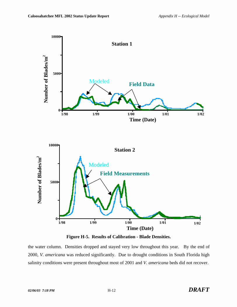
Caloosahatchee MFL 2002 Status Update Report Appendix H -- Ecological Model
02/06/03 7:18 PM H-12 DRAFT
Figure H-5. Results of Calibration - Blade Densities.
the water column. Densities dropped and stayed very low throughout this year. By the end of
2000, V. americana was reduced significantly. Due to drought conditions in South Florida high
salinity conditions were present throughout most of 2001 and V. americana beds did not recover.
1/98 1/99 1/00 1/01 1/02
Time (Date)
0
5000
10000
Modeled Field Data
Num
ber
of B
lade
s/m
2
1/98 1/99 1/00 1/01 1/02Time (Date)
0
5000
10000
MMooddeelleedd
Field Measurements
Num
ber
of B
lade
s/m
2
Station 1
Station 2Station 2
Station 1

Caloosahatchee MFL 2002 Status Update Report Appendix H -- Ecological Model
02/06/03 7:18 PM H-13 DRAFT
Figure H-6. Results of Calibration - Blade Densities.
Station 1
1/98 1/99 1/00 1/01 1/02
Time (Date)
0
0.5
1 1. Light Effect 2:Salinity Effect 3: Temperature Effect
1
2
1/98 1/99 1/00 1/01 1/02Time (Date)
0
0.5
12: Salinity Effect 3:Temperature Effect
Station 2
2
1
3
1. Light Effect
1. Light Effect
3

Caloosahatchee MFL 2002 Status Update Report Appendix H -- Ecological Model
02/06/03 7:18 PM H-14 DRAFT
Figure H-7. Results of Calibration- Salinity, Light, and Temperature Effects for Blades.
Station 1
1/98 1/99 1/00 1/01 1/02Time ( Date)
0
0.5
11: Light Effect 2: Salinity Effect 3: Temperature Effect
1
2
3
Station 2
1/98 1/99 1/00 1/01 1/02
Time (Date)
0
0.5
12: Salinity Effect 1: Light Effect 3:Temperature Effect
1
2
3
1. Light Effect

Caloosahatchee MFL 2002 Status Update Report Appendix H -- Ecological Model
02/06/03 7:18 PM H-15 DRAFT
At Station 1, the modeled computations predict field measurements reasonably well for 1998 and
1999. However the modeled results over-predict V. americana densities in the years 2000, 2001.
The complete loss of V. americana 2001 is not well represented in the model computation at
Station 1. At Station 2, the modeled results compare reasonably for all years (1998-2001), with a
slight under- estimation of densities occurring in 1999. The calibration data set at Station 2
illustrates the importance of both salinity and light on V. americana growth in the Estuary. In
2000 a severe light limitation occurs and although the salinity and temperature become very
favorable for growth immediately subsequent to the light restriction, V. americana does not
recover that year. In 2001, severe salinity conditions are apparent and prevent growth even
though light and temperature return to near optimums levels for growth (Figures H4 to H-7).
Temperatures are below known growth minimums for V. americana (Wilkinson, 1963) at Station
2 in the initial two months of the year (14oC) which may also have been inhibitory to growth/
establishment of this year. The temperature calculation does not specify a minimum value and
may overestimate density at very low temperatures (Figures H-6 and H-7).
Assumptions and Limitations: Calibration
1. Nutrients or other water quality parameters are not represented in the model and assumed
to be constant.
2. No epiphytic growth is considered. This would require considerations for nutrient cycling
to be added to model.
3. A reduced carrying capacity coefficient (maximum density coefficient) is necessary at
Station 1 relative to Station 2. This result indicates that factor(s) other than salinity, light,
or temperature may be impacting growth potential at this location. Possibilities include:
sediment characteristic(s) such as type, composition, nutritional status, slope, and toxics
and/ or physical characteristics such as depth, angle, flow velocity, grazing or other
physical disturbance. Future investigation is needed to determine the cause of this
difference.
4. It is assumed that a viable seed bank is present for population reestablishment after a
significant decline and there is no lag period for growth to commence once

Caloosahatchee MFL 2002 Status Update Report Appendix H -- Ecological Model
02/06/03 7:18 PM H-16 DRAFT
environmental conditions become favorable. No over-wintering buds for V. americana
have been found in Caloosahatchee Estuary and it is assumed that reestablishment occurs
by exclusively by seed germination. Population factors representing seed production or
dispersal are not represented in the model.
5. Light availability is calculated based on the light reaching the bottom. This is an
appropriate assumption for immature plants with leaves near the bottom. However, this
assumption may underestimate available light to larger more mature plants with leaves
extending up into the water column.
6. The P/I relationship and associated parameters (i.e. Ik) is assumed to remain the same
throughout all possible environmental conditions.
7. The various components that cause changes in water transparency (i.e. color, algal
blooms, suspended solids) are not differentiated. The effect is assumed to be the same
for all types of light reductions as measured by secci disk depth.
8. Grazing or other potential physical disturbances are not explicitly represented in the
model.
9. The effect of temperature changes on productivity is assumed to remain the same
throughout all possible environmental conditions (such as salinity or light changes).
10. The temperature minimum is not explicitly represented in the temperature formulation
and may overestimate growth if temperatures fall below the minimum growth
temperatures.
Sensitivity Analysis
Input Data
The quality, type, location and variability associated with the input data are important
considerations when interpreting model results. Field measurements should be used whenever
possible and the error associated with obtaining and processing the measurements should always
be considered. Unfortunately, creating input files using field data from the locations under

Caloosahatchee MFL 2002 Status Update Report Appendix H -- Ecological Model
02/06/03 7:18 PM H-17 DRAFT
consideration is not always possible. This may be the case when: there is limited field data in the
area of interest, for long-term simulations, and for future scenario analysis. Developing
approximations for input data during years when field data is not available is often necessary.
However, this introduces an additional source of error in the analysis. The potential impact of
using a form of input approximation (averaged data input files) verses field data during the 4-
year calibration period is illustrated by substituting the calibration files with the following:
• daily salinity input calculated from a regression model (Appendix F),
• 4-year water transparency averaged input files,
• 4-year temperature averaged input files.
In the latter two instances, the averaged input file was developed by averaging the four years
calibration data to create one “average year” input file.
Parameters
The sensitivity of input parameters is an additional factor to consider. Constant values obtained
from the literature are used in both the temperature and light functions. These values were
obtained under defined experimental conditions and do not necessarily represent the range of
conditions possible in the Caloosahatchee Estuary. Sensitivity analysis for the following
parameters are provided:
• Light saturation (Ik),
• Optimum temperature,
• Maximum temperature,
• Q10 coefficient used in temperature equation.
Sensitivity Analysis Discussion
For discussion purposes blade densities are specifically discussed in the sensitivity analysis.
The same analyses were performed for shoot densities with comparable results (data not shown.)

Caloosahatchee MFL 2002 Status Update Report Appendix H -- Ecological Model
02/06/03 7:18 PM H-18 DRAFT
Salinity
Use of salinity data interpolated from the field data (input to the calibration runs) or salinity input
from the regression model, (Appendix F) does not produce a significant impact on V. americana
densities at either Station 1 or Station 2 during the four-year of calibration period (Figures H-8
and H- 9).
Light
The use of an averaged annual secci disk depth input file produced differences compared to the
calibrated model, which uses field measurements at both Station 1 and 2. (Figure H-10). The
blade density at both stations 1 and 2 is overestimated in 2000 and 2001. This is due to
underestimation of true water transparency using the averaged annual input file and illustrates
the importance of light limitation in these two years. Additionally at Station 2, the average
annual input file results in an underestimation of blade density in 1998 due to increased water
transparency relative to the four-year average (Figure H-11).
The averaged annual data files resulted in secci disk depths ranging from 0.9 m to 1.3 m at
Station 1 during the course of a year. The field data for the four-year calibration period shows a
greater degree in variability in measurements ranging from 0.5 to 1.75m (Figure H-11). At
Station 2, field measurements fall below 0.3m (data not shown). Thus the averaged data files do
not account for the variability and extremes events such as phytoplankton blooms or highly
colored water from basin discharge nor do they represent years that have very high water
transparency such as that of 1998. It is these extreme values that may have the greatest impacts
on V. americana growth.
The parameter Ik derived from P/I relationships is used directly in the determination of the light
effect. The sensitivity of blade density to raising or lowering Ik within ranges reported in the
literature (Harley and Findlay, 1994) is shown in Figure H-12. At both stations variations in Ik
simply raised or lowered the peak density values. The model currently assumes this value to be
constant over all environmental conditions. As discussed previously, research has indicated that
P/I relationships (and thus Ik) are dynamic and can potentially change with water temperature,
salinity, and prior exposure. Due to lack of quantifiable information available at the present time,
this value remains constant in the current model. Analysis of recent experimental work (Hunt et

Caloosahatchee MFL 2002 Status Update Report Appendix H -- Ecological Model
02/06/03 7:18 PM H-19 DRAFT
Figure H-8: Results of modeled V. americana Blade Densities Using Different Salinity Input
Station 1
1/98 1/99 1/00 1/01 1/02
Time (Date)
0
5000
10000 N
umbe
r of
Bla
des/
m2
Calibration Salinity InputRegression Model Salinity Input
Station 2
1/98 1/99 1/00 1/01 1/02Time (Date)
0
5000
10000
Num
ber
of B
lade
s/m
2
Calibration Salinity Input
Regression Model Salinity Input
Calibration Salinity Input
Calibration Salinity Input

Caloosahatchee MFL 2002 Status Update Report Appendix H -- Ecological Model
02/06/03 7:18 PM H-20 DRAFT
Figure H-9. Comparison of Salinity Input Data
Station 1
1/98 1/99 1/00 1/01 1/02Time (Date)
0
30Sa
linit
y (p
pt) Calibration Salinity Input
Station 2
1/98 1/99 1/00
1/01 1/02Time (Date)
0
15
30
Salin
ity
(ppt
)
Calibration Salinity Input
Regression Model Salinity Input
2
Calibration Salinity Input
Regression ModelSalinity Input
Calibration Salinity Input
Station 1
Station 2

Caloosahatchee MFL 2002 Status Update Report Appendix H -- Ecological Model
02/06/03 7:18 PM H-21 DRAFT
Figure H-10: Results of modeled V. americana Blade Densities Using Different WaterTransparency Input.
Station 1N
umbe
r of
Bla
des/
m2
1/98 1/99 1/00 1/01 1/02
Time (Date)
0
5000
10000
Field Data Secci Disk Input Used in Calibration
Averaged Secci Disk Input
Station 2
Num
ber
of B
lade
s/m
2
1/98 1/99 1/00 1/01 1/02Time (Days)
0
5000
10000
Field Data Secci Disk Input Used in Calibration
Averaged Secci Disk Input
Station 1
Station 2
Field Data Secci Disk Input Used in Calibration
Field Data Secci Disk Input Used in Calibration

Caloosahatchee MFL 2002 Status Update Report Appendix H -- Ecological Model
02/06/03 7:18 PM H-22 DRAFT
Figure H-11: Comparison of Water Transparency Input Data.
Station 1Se
cci D
isk
dept
h (m
)
1/98 1/99 1/00 1/01 1/02
Time (Date)
0
1
2 Field Data Used for Calibration Averaged Data
Station 2
Secc
i Dis
k D
epth
( m
)
1/98 1/99 1/00 1/01 1/02Time (Date)
0
1
2 Field Data Used for CalibrationAveraged Data
Field Data Used in Calibration
Field Data Used in Calibration
Station 2

Caloosahatchee MFL 2002 Status Update Report Appendix H -- Ecological Model
02/06/03 7:18 PM H-23 DRAFT
Figure H-12: Light Saturation Parameter (Ik) Sensitivity for Blade Density.
Station 1
Num
ber
of B
lade
s/m
2
1/98 1/99 1/00 1/01 1/02
Time (Date)
0
5000
10000
1 : Ik = 200 2: Ik = 150 3: Ik = 250
1
23
Station 2
Num
ber
of B
lade
s/m
2
1/98 1/99 1/00 1/01 1/02
Time (Date)
0
5000
10000
1 : Ik = 200 2: Ik = 150 3 : Ik = 250
1 2
3
Station 1
Station 2

Caloosahatchee MFL 2002 Status Update Report Appendix H -- Ecological Model
02/06/03 7:18 PM H-24 DRAFT
al. 2002) is expected to produce refinements in the way the P/I curve is formulated: both in terms
of differences in respiration and photosynthesis under high and low salinity as well as prior light
exposure/acclimation.
Temperature
Comparison of averaged temperature input file and the field data does not show a significant
impact on the computed V. americana densities for either Station 1 or Station 2 during the four-
year calibration period (Figures H-13 and H- 14). In addition, raising optimal growth
temperature to 36 oC, reducing maximum growth temperature to 45 oC or changing the Q10
values did not have significant impacts (data not shown).
31-Year Scenarios
To evaluate plans for watershed management, V. americana computations for Station 1 and
Station 2 were generated under the following two scenarios:
• 31-year period simulation using 1995 Base Case condition flows,
• 31-year period using CERP D13R project condition flows.
Data Needs
The input data is summarized in Table H-3. In both simulations, daily salinity predicted by a
regression equation derived from a 3-D hydrodynamic model (Appendix F), served as input to
the V. americana model. Input water temperature, secci disk depth, and PAR were determined
using averaged annual data sets (determined from the calibration period). Therefore salinity was
the only dynamic variable in these simulations and the remaining inputs were maintained as
“average conditions” throughout each annual cycle.
Table H-3. Input Data Summary For 31-Year Scenarios
INPUT DATA SOURCE (FREQUENCY)
Salinity (ppt) Regression model based on hydrodynamic model (daily avg.)see Appendix F this document
Water Transparency (m) Averaged data set used for calibration from 1998-2001 (monthly)Incident PAR (µE/s*m2) Averaged data set used for calibration from 1998-2001 (average daily)Water Temperature (oC) Averaged data set used for calibration from 1998-2001 (monthly)

Caloosahatchee MFL 2002 Status Update Report Appendix H -- Ecological Model
02/06/03 7:18 PM H-25 DRAFT
Figure H-13: Results of Modeled V. americana Blade Densities Using Different m WaterTemperature Input
Station 1N
umbe
r of
Bla
des/
m2
1/98 1/99 1/00 1/01 1/02
Time (Date)
0
5000
10000
Field Water Temperature Data Used In Calibration
Averaged Water Temperature Data
Station 2
Num
ber
of B
lade
s/m
2
1/98 1/99 1/00 1/01 1/02
Time (Date)
0
5000
10000
Field Water Temperature Data Used in Calibration
Averaged Water Temperature Data
Field Water Temperature Data Used in Calibration
Field Water Temperature Data Used in Calibration
Station 1
Station 2
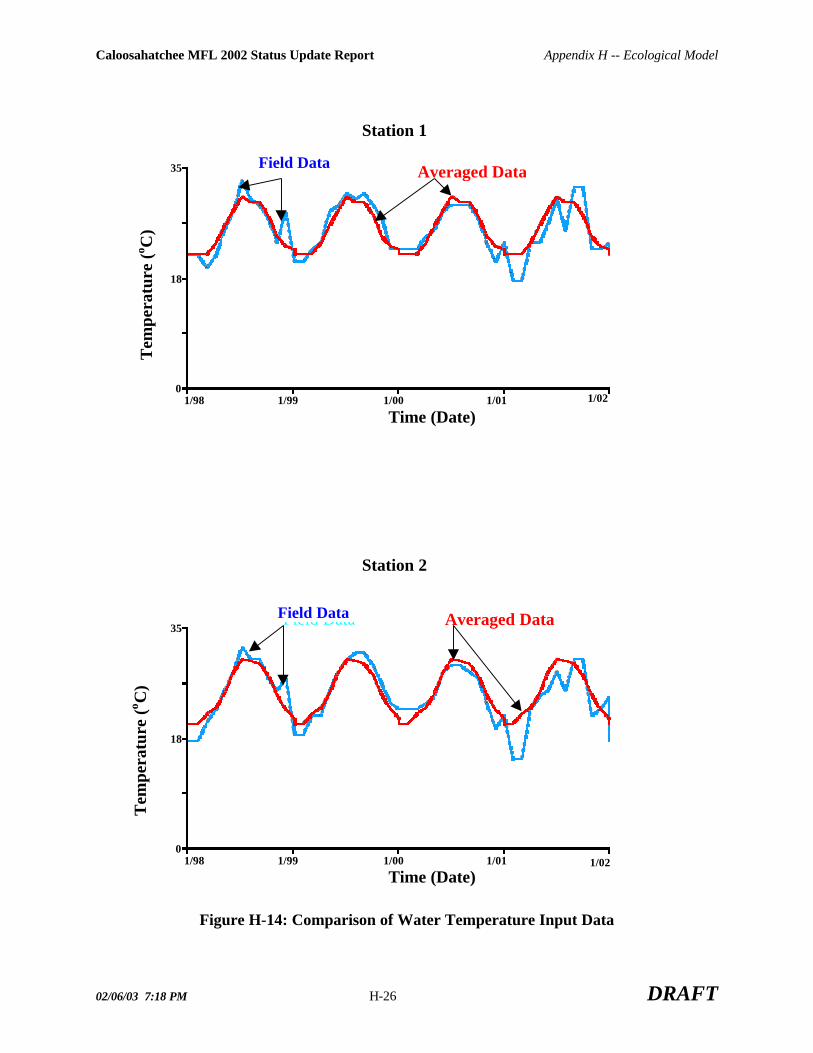
Caloosahatchee MFL 2002 Status Update Report Appendix H -- Ecological Model
02/06/03 7:18 PM H-26 DRAFT
Figure H-14: Comparison of Water Temperature Input Data
Station 1
Station 2
Tem
pera
ture
(o C)
1/98 1/99 1/00 1/01 1/02
Time (Date)
0
18
35 Field Data Averaged Data
Tem
pera
ture
(o C)
1/98 1/99 1/00 1/01 1/02Time (Date)
0
18
35Field Data Averaged Data
Field Data
Field Data

Caloosahatchee MFL 2002 Status Update Report Appendix H -- Ecological Model
02/06/03 7:18 PM H-27 DRAFT
The simulations using the CERP D13R project flow conditions show more favorable V.
americana densities than the 95 base case at both Station 1 and Station 2 (Figures H-15 and H-
16). Specifically, there is a 68% increase in total number of shoots produced for the 31 year
period modeled at Station 1 and 51 % increase at Station 2 in the D13R scenario compared to the
95 base case. For blade density, there is a 74% increase at Station 1 and 23% at Station 2 in the
D13R scenario compared to the 95 base case.
Assumptions and Limitations
In addition to the general model limitation and assumptions stated previously there are further
considerations when evaluting the outcome of the 31-year scenarios.
1. Due to the fluctuation of salinity within small timesteps, daily input is preferred. In order
to accommodate this scale, salinity input to the V. americana model was provided using a
regression equation model derived from a 3-D Hydrodynamic model (Appendix F).
Thus the model is calibrated using salinity data that is predicted from a model and carries
with it the errors associated with this input data.
2. The model also requires direct input data for water temperature, incident PAR and water
transparency. Field measurements of these variables are directly input in the four-year
calibration runs. In the 31 scenarios, these three variables are estimated based on yearly
averages from the 4-year calibration data and are assumed to be constant from year to
year. Thus, there are no light-limiting conditions or temperature extremes represented in
the 31-year scenarios. As illustrated in the sensitivity analysis, use of the averaged
annual input files can result in differences in computed V. americana density than those
using dynamic field data (Figures H-10 and H-11). Specifically, a notable limitation of
the 31-year simulations is that these simulations do not represent deviations in
transparency that may occur in the upper portions of the Estuary. Such deviations that
would be expected to negatively impact growth may occur due to algal blooms, highly
colored discharges or sediment transport. Specifically the scenario, which is occurs in the
third year of calibration (2000) is not represented by the 31-year scenarios shown
(Figures H-4 to H7). Similarly, periods of high water clarity such as are represented in

Caloosahatchee MFL 2002 Status Update Report Appendix H -- Ecological Model
02/06/03 7:18 PM H-28 DRAFT
Station 1
Figure H-15: Results of 31-Year Scenarios - Shoot Density
0
250
500
750
1000
1250
1500
Jan-
65
Jan-
67
Jan-
69
Jan-
71
Jan-
73
Jan-
75
Jan-
77
Jan-
79
Jan-
81
Jan-
83
Jan-
85
Jan-
87
Jan-
89
Jan-
91
Jan-
93
Jan-
95
Time
Num
ber
of S
hoot
s/m
2
D13R 1995 Base
0
2000
4000
6000
8000
10000
Jan-
65
Jan-
67
Jan-
69
Jan-
71
Jan-
73
Jan-
75
Jan-
77
Jan-
79
Jan-
81
Jan-
83
Jan-
85
Jan-
87
Jan-
89
Jan-
91
Jan-
93
Jan-
95
Time
Num
ber
of B
lade
s/m2
D13R 1995 Base

Caloosahatchee MFL 2002 Status Update Report Appendix H -- Ecological Model
02/06/03 7:18 PM H-29 DRAFT
Station 2
Figure H-16: Results of 31-Year Scenarios - Blade Density
0
250
500
750
1000
1250
1500
Jan-
65
Jan-
67
Jan-
69
Jan-
71
Jan-
73
Jan-
75
Jan-
77
Jan-
79
Jan-
81
Jan-
83
Jan-
85
Jan-
87
Jan-
89
Jan-
91
Jan-
93
Jan-
95
Time
Num
ber
of S
hoot
s/m2
D13R 1995 Base
0
2000
4000
6000
8000
10000
Jan-
65
Jan-
67
Jan-
69
Jan-
71
Jan-
73
Jan-
75
Jan-
77
Jan-
79
Jan-
81
Jan-
83
Jan-
85
Jan-
87
Jan-
89
Jan-
91
Jan-
93
Jan-
95
Time
Num
ber
of B
lade
s/m2
D13R 1995 Base

Caloosahatchee MFL 2002 Status Update Report Appendix H -- Ecological Model
02/06/03 7:18 PM H-30 DRAFT
the calibration period during the summer of 1998 may produce exceptional growth conditions
and is not represented in the 31-year simulations.
3. The water depth at each site is assumed to be constant over the 31-year period.
Future Improvements
Due to the limited amount of time available to construct and calibrate the V. americana model,
improvements are anticipated. It is necessary that all field monitoring be continued and the
calibration period be extended to include the new data. The extended calibration period will
permit improved prediction of V. americana recovery after severe conditions. Additional input
data and information concerning the growth and survival of V. americana in the Caloosahatchee
Estuary will be required to make the model more robust. Information is needed for validation of
some existing equations, refinements to salinity, light and temperature effects as well as
development of additional state variables. Equations representing additional important ecosystem
components will be incorporated into the model. Potential examples include: sediment
characteristics, current, sediment diagensis, biogeochemical rate processes, sulfide, flowering,
and competition for light and nutrients by plankton and microphytobenthos. The relative
importance of these variables and the information needed to quantify these effects are currently
under review. Additional forcing functions may be added such as color, chlorophyll-a,
suspended solids, and nutrients. State variables describing additional plant morphologies such as
canopy height, and below ground biomass may also be added. Future work, outlined below, falls
into three broad categories, data analysis, model development, and experimental or site work.
Data analysis
• Develop a method to predict variation in water transparency for long-term or other
simulations.
• Quantify input data error and perform additional sensitivity analysis.
• Develop relationships to relate mass to blade and shoot densities, and blade length with
existing data.

Caloosahatchee MFL 2002 Status Update Report Appendix H -- Ecological Model
02/06/03 7:18 PM H-31 DRAFT
Model Development
• Quantify existing experimental work (Hunt et al., 2002) and develop improved algorithms
for light and salinity.
• Incorporate blade length as a state variable to more accurately represent light availability
for mature plants.
• Add nutrient cycling/ water quality impacts.
• Add population and demographic characteristics to describe seed production and dispersal.
Experimental /Site Work
• General areas of data needs include: above and below ground biomass measurements at
existing sampling stations, levels and influence of pore water salinity and sulfide, and
direct light attenuation measurements. Field measurements should be obtained under
differing environmental conditions.
• Identify the factor(s) responsible for reduced carrying capacity in Station 1 relative to
Station 2. Some factor(s) other than light attenuation (as measured by secci disk), salinity
or temperature governed the growth of V. americana at Stations 1 during the four-year
calibration period.
• Develop criteria and cues (including lag times) for reestablishment of V. americana
growth after population has been substantially reduced. The assumption that
reestablishment occurs via a seedbank should be verified.
CONCLUSIONS
The ecological model described, although still in the developmental stages, synthesizes known
information about the growth and survival of V. americana in the Upper Caloosahatchee Estuary.
Calibration of the 4- year period 1998-2001 indicates reasonable agreement with field data. It is
expected that improvements will be forthcoming as the model is further developed.

Caloosahatchee MFL 2002 Status Update Report Appendix H -- Ecological Model
02/06/03 7:18 PM H-32 DRAFT
The four primary criticisms (listed previously) of the peer reviewers for the Draft MFL
Document of September 2000 (SFWMD, 2000) are being addressed by the development of the
ecological model. This model includes the effects of multiple environmental variables: salinity,
light, and temperature. Additional variables such as nutrient cycling and sediment diagenesis will
be added to the model as appropriate. The issue of spatial variability is addressed by verifying
and calibrating the model at two locations within the Upper Caloosahatchee Estuary. Additional
locations further downstream may be added in the future. In terms of demographic variability,
the model predicts several measures of growth including shoot density, blade density and,
biomass. The capability to predict average canopy height will also be included in the future.
Long-term (31-year) simulations with variable input salinity regimes derived from a
hydrodynamic model are presented addressing another criticism. Finally the panels concern
regarding the annual shoot recovery densities set as constant has also been addressed. The
current model allows for the user to either input any desired starting density or calculate a
density given a previous years growth by performing multiple-year simulations.
The model can be used as a tool to assess management strategies in the Upper Caloosahatchee
Estuary. Information generated by the model can eventually be used to optimize timing and
quantity of freshwater releases to the upper estuary as indicated by MFL criteria. The model can
also be used to identify important factors influencing V. americana growth and survival.
Simulations can be used to test hypothesis concerning the influence of freshwater flows on V.
americana productivity and survival. Mechanisms responsible for habitat decline can be
elucidated and conditions required for restoration and survival can be evaluated. A set of habitat
requirements for V. americana survival and growth for target densities can be then established at
different locations within the Upper Caloosahatchee Estuary. Compilation of existing data and
sensitivity analysis within the model framework can highlight areas of data needs and be used
guide and prioritize future work efforts.
Caloosahatchee MFL 2002 Status Update Report Appendix H -- Ecological Model
02/06/03 7:18 PM H-33 DRAFT
REFERENCES
Barko, J. W., D. G. Hardin and M. S. Matthews. 1982. Growth and morphology of submergedfreshwater macrophytes in relation to light and temperature. Canadian I. Bot. 60:877-887
Barko, J. W., D. G. Hardin, and M. S. Matthews. 1984. Interactive Influences of Light andTemperature on the Growth and Morphology of Submerged Freshwater Macrophytes.Technical Report A-84-3, U. S. Army Corps of Engineers, Waterways ExperimentalStation, Vicksburg, Miss. 24 pp
Barko, J. W., R. M. Smart, and D. G. McFarland. 1991. Interactive effects of environmentalconditions on the growth of submerged aquatic macrophytes. Journal of FreshwaterEcology 6(2):199-207
Blackman, F. F. 1905. Optima and limiting factors. Ann. Bot. 19: 281-295
Bourn, W. S. 1932. Ecological and physiological studies on certain aquatic angiosperms. Con-trib. Boyce Tompson Inst. 4:425-496
Bulthuis, D.A. 1987. Effects of temperature on photosynthesis and growth of seagrasses.Aquatic Botany. 27 pp 27-40.
Dawes, C. J. and D. A. Tomasko. 1988. Depth distribution of Thalassia testudinum in twomeadows on the west coast of Florida: a difference in effect of light availability. Mar.Ecol. 9: 123-130
Dennison, W. C. 1990. Photosynthetic and growth responses of tropical and temperate seagrassesin relation to secchi depth, light attenuation and daily light period. In The LightRequirements of Seagrasses: Results and Recommendations of a Workshop Convened toExamine the Capability of Water Quality Criteria, Standards and Monitoring Programs toProtect Seagrasses from Deteriorating Water Transparency. November 7-8, 1990 at SouthFlorida Water Management District. Editors, Kenworthy, J. D.and D.E. Haunert. Pp 82-85
Drew, E. A. 1978. Factors affecting photosynthesis and its seasonal variation in in the seagrassesCymodocea nodosa (ueria) Aschers, and Posidonia oceanica (L.) Delile in theMediterranean. J. Exp. Mar. Biol. Ecol. 31:173-194
Doering, P.H., Chamberlain, R.H., Donohue, K.M., and A.D. Steinman. 1999. Effect of salinityon the growth of V. americana Michx. from the Caloosahatchee Estuary, FL. FloridaScientist. 62 (2):89-105
Edwards, R. E., W. Lung, P.A. Montagna, and H. L. Windom. 2000. Caloosahatchee MinimumFlow, Final Review Report, Peer Review Panel. September 27-29. 30pp
Fourqurean, J.W. and. J.C. Zieman. 1991. Photosynthesis, respiration and whole plant carbonbudget of the seagrass Thalassia testudinum. Marine Ecology Progress Series. 69:161-170
Giesen, W. B. J. T., M. M. van Katijk, andC. Den Hartog. 1990. Eelgrass condition and turbidityin the Dutch Wadden Sea. Aquatic Botany. 37:71-85

Caloosahatchee MFL 2002 Status Update Report Appendix H -- Ecological Model
02/06/03 7:18 PM H-34 DRAFT
Harley, M.T., and S. Findlay. 1994. Photosynthesis - Irradiance relationships for three species ofsubmerged macrophytes in the tidal freshwater Hudson River. Estuaries. 17 (1B):200-205
Hunt, G. S. 1963. Wildcelery in the lower Detroit River. Ecology 44:360-370
Hunt, M. J. et al. 2002. Unpublished data
Kimber, A., C. E. Korschgen, and A. G. Van der Valk. 1995. The distribution of Vallisneriaamericana seeds and seedling light requirements in the Upper Mississippi River.Canadian Journal of Botany 73(12):1966-1973.
Lowden, R. M. 1982. An approach to the taxonomy of Vallisneria L. (hydrocharitaceae). AquaticBotany. 13:269-298
Meyer, B. S., F. H. Bell, L. C. Thompson, and E. I. Clay. 1943. Effect of depth of imersion onapparent photosynthesis in submerged vascular aquatics. Ecology 24:393-399
O’Neill, R.V., R.A. Goldstein, H.H. Shugart, and J.B. Manki. 1972. Terrestrial EcosystemEnergy Model. U. S. IBP Eastern Deciduous Forest Biome Memo Report Number 72-19.Oak Ridge National Laboratory, Oak Ridge, Tennessee, USA.
Qiu, C. Appendix F. This document.
SFWMD. 2000. Technical Documentation to Support Development of Minimum Flows andLevels for the Caloosahatchee River and Estuary. Water Supply Division. September 6,2000 Draft.
Smart, R. M., and J. D. Dorman. 1993. Latitudinal differences in the growth strategy of asubmerged aquatic plant: ecotype differences in Vallisneria americana? Bull.Ecol. Soc.Am. 74(Suppl.):439
Titus, J.E. and M.S. Adams. 1979. Coexistence and the comparative light relations of thesubmerged macrophytes Myriophylulum spicatum L. and Vallisneria americana Michx.Oecologia. 40:273-286.
USEPA. 1992. Chesapeake Bay Submerged Aquatic Vegetation Habitat Requirements andRestoration Targets: A Technical Synthesis, Annapolis, MD, December, 1992. Printed bythe United States Environmental Protection Agency for the Chesapeake Bay Program,contract number 68-WO-00043, 15-19.
Wilkinson, R. E. 1963. Effects of light intensity and temperature on the growth of WaterStargrass, Coontail, and Duckweed. Weeds. 11:287-289.