technical analysis of can slim stocks
TRANSCRIPT

Technical Analysis of CAN SLIM Stocks
A Major Qualifying Project Report
Submitted to the Faculty of
Worcester Polytechnic Institute
In Partial Fulfillment of the Requirements for a
Degree of Bachelor of Science
by
Belin Beyoglu Martin Ivanov
Advised by
Prof. Michael J. Radzicki
May 1, 2008

Table of Contents
Table of Figures .............................................................................................................. 7
Table of Tables ................................................................................................................ 9
1. Abstract .................................................................................................................. 10
2. Introduction and Statement of the Problem .......................................................... 11
3. Background Research ............................................................................................ 13
3.1. Fundamental Analysis .................................................................................... 13
3.1.1. Earnings per Share (EPS) ........................................................................ 14
3.1.2. Price-to-Earnings Ratio (P/E) ................................................................. 14
3.1.3. Return on Equity (ROE) .......................................................................... 15
3.2. Technical Analysis .......................................................................................... 15
3.2.1. The Bar Chart .............................................................................................. 17
3.2.2. Average True Range (ATR) ...................................................................... 17
3.3. CAN SLIM ....................................................................................................... 18
3.3.1. C: Current Earnings Growth .................................................................... 18
3.3.2. A: Annual Earnings Growth ..................................................................... 19
3.3.3. N: New Products, New Services, New Management, New Price Highs .. 19
3.3.4. S: Supply and Demand ............................................................................ 19
3.3.5. L: Leader or Laggard ................................................................................ 20
3.3.6. I: Institutional Sponsorship ..................................................................... 20
3.3.7. M: Market ................................................................................................. 20
Page | 2
3.3.8. Our CAN SLIM Stock Selection ............................................................... 21
3.4. TradeStation ................................................................................................... 22
3.5. Performance Measurements........................................................................... 22
3.5.1. Expectunity and System Quality Measurement ...................................... 22
3.5.2. Monte Carlo Analysis ............................................................................... 23
4. Complete Trading Strategies ................................................................................. 25
4.1. Set-up .............................................................................................................. 26
4.2. Entry ............................................................................................................... 27
4.3. Exit with a profit ............................................................................................. 28
4.4. Exit with a loss (Money management stop) ................................................... 29
4.5. Money Management ....................................................................................... 29
5. Back-Testing using TradeStation .......................................................................... 30
5.1. Overview of the Back-Testing Procedure ....................................................... 30
5.2. Moving Average Crossover ............................................................................. 31
5.3. Bollinger Bands ............................................................................................... 32
5.4. Keltner Channel .............................................................................................. 33
5.5. Volume Breakout ............................................................................................ 34
5.6. Donchian Channel 20-Day and 55-Day ......................................................... 34
6. Results Attained from Back-testing ...................................................................... 36
6.1. Bollinger Bands ............................................................................................... 36
6.1.1. TradeStation Settings .............................................................................. 36
6.1.2. AAPL: Apple Inc. (NASDAQ) ................................................................... 37
Page | 3
6.1.3. MTL: Mechel OAO (NYSE) ...................................................................... 38
6.1.4. RIMM: Research in Motion Limited (NASDAQ) .................................... 38
6.1.5. Equity Curve ............................................................................................. 39
6.1.6. Monte Carlo Simulation Results at a 95% Confidence ............................40
6.1.7. Raw System Quality Results ....................................................................40
6.2. Volume Breakout ............................................................................................ 41
6.2.1. TradeStation Settings .............................................................................. 41
6.2.2. AAPL: Apple Inc. (NASDAQ) ................................................................... 42
6.2.3. MTL: Mechel OAO (NYSE) ...................................................................... 43
6.2.4. RIMM: Research in Motion Limited (NASDAQ) .................................... 43
6.2.5. Equity Curve ............................................................................................. 44
6.2.6. Monte Carlo Simulation Results at a 95% Confidence ............................ 45
6.2.7. Raw System Quality Results .................................................................... 45
6.3. Moving Average Crossover ............................................................................. 46
6.3.1. TradeStation Settings .............................................................................. 46
6.3.2. AAPL: Apple Inc. (NASDAQ) ................................................................... 47
6.3.3. MTL: Mechel OAO (NYSE) ...................................................................... 48
6.3.4. RIMM: Research in Motion Limited (NASDAQ) .................................... 48
6.3.5. Equity Curve ............................................................................................. 49
6.3.6. Monte Carlo Simulation Results at a 95% Confidence ............................ 50
6.3.7. Raw System Quality Results .................................................................... 50
6.4. Keltner Channel .............................................................................................. 51
Page | 4
6.4.1. TradeStation Settings .............................................................................. 51
6.4.2. AAPL: Apple Inc. (NASDAQ) ................................................................... 51
6.4.3. MTL: Mechel OAO (NYSE) ...................................................................... 52
6.4.4. RIMM: Research in Motion Limited (NASDAQ) .................................... 53
6.4.5. Equity Curve ............................................................................................. 53
6.4.6. Monte Carlo Simulation Results at a 95% Confidence ............................ 54
6.4.7. Raw System Quality Results .................................................................... 55
6.5. Donchian Channel 20-day .............................................................................. 55
6.5.1. TradeStation Settings .............................................................................. 55
6.5.2. AAPL: Apple Inc. (NASDAQ) ................................................................... 56
6.5.3. MTL: Mechel OAO (NYSE) ...................................................................... 57
6.5.4. RIMM: Research in Motion Limited (NASDAQ) .................................... 57
6.5.5. Equity Curve ............................................................................................. 58
6.5.6. Monte Carlo Simulation Results at a 95% Confidence ............................ 59
6.5.7. Raw System Quality Results .................................................................... 59
6.6. Donchian Channel 55-days .............................................................................60
6.6.1. TradeStation Settings ..............................................................................60
6.6.2. AAPL: Apple Inc. (NASDAQ) ...................................................................60
6.6.3. MTL: Mechel OAO (NYSE) ...................................................................... 61
6.6.4. RIMM: Research in Motion Limited (NASDAQ) .................................... 61
6.6.5. Equity Curve ............................................................................................. 62
6.6.6. Monte Carlo Simulation Results at a 95% Confidence ............................ 63
Page | 5

6.6.7. Raw System Quality Results .................................................................... 63
7. Comparison of the Strategies ................................................................................ 64
7.1. System Quality Comparison ........................................................................... 64
7.2. Monte Carlo Simulation Comparison ............................................................ 65
8. Conclusion ............................................................................................................. 66
9. Further Work ......................................................................................................... 67
10. References .......................................................................................................... 68
11. Appendixes ......................................................................................................... 70
11.1. Moving Average Crossover Strategy EasyLanguage Code ............................. 70
11.2. Donchian Channel Strategy EasyLanguage Code ....................................... 71
11.3. Keltner Channel Strategy EasyLanguage Code ........................................... 72
11.4. Bollinger Bands Strategy EasyLanguage Code ........................................... 73
11.5. Volume Breakout Strategy EasyLanguage Code ......................................... 74
11.6. CAN SLIM Stock Selection Indicator EasyLanguage Code ........................ 75
11.7. CAN SLIM Stock Selection (Symbols) ........................................................ 79
Page | 6
Table of Figures
Figure 1: Bar Chart (What Are Charts?) ...................................................................... 17
Figure 2- Trades Generated by Bollinger Bands, AAPL .............................................. 37
Figure 3 - Trades Generated by Bollinger Bands, MTL ............................................... 38
Figure 4 - Trades Generated by Bollinger Bands, RIMM ............................................ 38
Figure 5 - Equity Curve Generated by Bollinger Bands ............................................... 39
Figure 6 - Monte Carlo Results of Bollinger Bands at a 95% Confidence ...................40
Figure 7 - Trades Generated by Volume Breakout, AAPL ........................................... 42
Figure 8 - Trades Generated by Volume Breakout, MTL ............................................ 43
Figure 9 - Trades Generated by Volume Breakout, RIMM ......................................... 43
Figure 10 - Equity Curve Generated by Volume Breakout .......................................... 44
Figure 11 - Monte Carlo Simulations Results for Volume Breakout at a 95%
Confidence .................................................................................................................... 45
Figure 12 - Trades Generated by Moving Average Crossover, AAPL .......................... 47
Figure 13 – Trades Generated by Moving Average Crossover, MTL ........................... 48
Figure 14 - Trades Generated by Moving Average Crossover, RIMM ......................... 48
Figure 15 - Equity Curve Generated by Moving Average Crossover ........................... 49
Figure 16 - Monte Carlo Simulation Results for Moving Average Crossover at a 95%
Confidence .................................................................................................................... 50
Figure 17 - Trades Generated by Keltner Channel, AAPL ........................................... 51
Figure 18 - Trades Generated by Keltner Channel, MTL ............................................ 52
Figure 19 - Trades Generated by Keltner Channel, RIMM .......................................... 53
Figure 20 - Equity Curve Generated by Keltner Channel ............................................ 53
Figure 21 - Monte Carlo Simulation Results for Keltner Channel at a 95% Confidence
...................................................................................................................................... 54
Page | 7
Figure 22- Trades Generated by Donchian Channel 20-Day, AAPL ........................... 56
Figure 23 - Trades Generated by Donchian Channel 20-Day, MTL ........................... 57
Figure 24 - Trades Generated by Donchian Channel 20-Day, RIMM ........................ 57
Figure 25 - Equity Curve Generated by Donchian Channel 20-Day ........................... 58
Figure 26 - Monte Carlo Simulation Results for Donchian Channel 20-Day at a 95%
Confidence .................................................................................................................... 59
Figure 27 - Trades Generated by Donchian Channel 55-Day, AAPL ..........................60
Figure 28 - Trades Generated by Donchian Channel 55-Day, MTL ............................ 61
Figure 29 - Trades Generated by Donchian Channel 55-Day, RIMM ......................... 61
Figure 30 - Equity Curve Generated by Donchian Channel 55-Day ........................... 62
Figure 31 - Monte Carlo Simulation Results for Donchian Channel 55-Day at a 95%
Confidence .................................................................................................................... 63
Page | 8

Table of Tables
Table 1 - TradeStation Settings for Bollinger Bands ................................................... 36
Table 2- System Quality Results for Bollinger Bands ..................................................40
Table 3 - TradeStation Settings for Volume Breakout ................................................. 41
Table 4 - System Quality Results for Volume Breakout .............................................. 45
Table 5 TradeStation Settings for Moving Average Crossover .................................... 46
Table 6 - System Quality Results for Moving Average Crossover ............................... 50
Table 7 - TradeStation Settings for Keltner Channel ................................................... 51
Table 8 - System Quality Results for Keltner Channel ................................................ 55
Table 9 - TradeStation Settings for Donchian Channel 20-day .................................. 56
Table 10 - System Quality Results for Donchian Channel 20-Day .............................. 59
Table 11 - TradeStation Settings for Donchian Channel 55-Day .................................60
Table 12 - System Quality Results for Donchian Channel 55-Day .............................. 63
Table 13 - System Quality Results ................................................................................ 64
Table 14 - Monte Carlo Simulation Results ................................................................. 65
Page | 9

1. Abstract
This MQP combines fundamental and technical analysis by adding value to the
CAN SLIM investment methodology through the concept of complete trading
strategies. We utilize the TradeStation trading platform to evaluate five set-ups -
Donchian channel 20-day and 55-day, Keltner channel, Bollinger bands, moving
average crossover and volume breakouts – by back-testing 559 CAN SLIM stocks for
2007. For comparison purposes we employ system quality calculations and Monte
Carlo analysis to assess the performance of each set-up.
Page | 10
2. Introduction and Statement of the Problem
$51 trillion. That’s how much the stock market’s value is estimated at, making it
about four times the size of the U.S. economy. Its significance as a part of the
American financial system cannot be downplayed. It has provided Americans with
immense profit opportunities, enabling them to buy a new house, send their child to
a top-tier university or retire early. These are dreams which each of us have but only
a few know the best path for realizing them. And how else given the seemingly
infinite number of investment instruments - stocks, bonds, all those exotic
derivatives, mutual funds, hedge funds… Most people do not have the courage NOT
to follow an analyst’s advice after watching CNBC or reading a free investment
newsletter. They simply do not believe they could have a greater return by investing
on their own and beating the average annual return of a mere 7.84% of the S&P 500
for the past 50 years. (Moneychimp) And in part, they are right. To be a successful
trader, you need to be disciplined, to learn to disregard all the headlines and analysts’
comments, taking emotions out of the game. You need to adhere to your own rules
under any circumstances. You need to decide what you trade, when you trade, how
you enter a position and how you exit it, when you take profits and when you stop
your losses.
The purpose of this MQP is to show individual investors a way to implement all
the above rules by introducing them to the development of complete trading
strategies. As with many other stock trading strategies, ours incorporates
fundamental and technical analysis. We have decided that the former has already
been perfected trough the CAN SLIM methodology created by William O’Neil (O'Neil,
2002) and offered by Investor’s Business Daily (IBD). That’s why we do not intend to
spend any more time deciding which stock has the necessary fundamental
Page | 11

characteristics but concentrate on the latter part of the equation. Bill O’Neil and IBD
provide the individual investor with a list of CAN SLIM stocks but they offer only
limited advice on when and how to buy or sell them. In our MQP we solve this issue
by using the TradeStation trading platform which allows for the testing of various
technical indicators on the CAN SLIM stocks.
In the first part of this report we will introduce you to the essence of fundamental
and technical analysis. We will cover those concepts we deem to be pertinent to this
MQP. After that we will guide you through the world of CAN SLIM stocks – what
they are, where you can find them and how we are going to use them. Then we will
introduce you to the complete trading strategies and their five steps – set-up, entry,
exit with a profit, exit with a loss and money management. In the end we will analyze
the CAN SLIM stocks for 2007 using TradeStation by testing five set-ups while
keeping the other aspects of the complete trading strategy constant. To compare the
performance of each set-up we will use system quality calculations and Monte Carlo
analysis which will allow us to differentiate between the strengths and weaknesses of
each strategy. Finally, we reach the conclusion that the trend-following moving
average crossover strategy combines the best out of the six strategies we back-test
with the CAN SLIM characteristics.
Page | 12
3. Background Research
3.1. Fundamental Analysis
Fundamental analysis is a method used to determine the value of a stock by
analyzing the financial data essential to the company with the goal of projecting
future price movements. Investors examine the company’s financials and operations
by looking at sales, earnings, dividends, growth potential, assets, debt, management,
products and competition, in order to verify if a stock should be bought or sold. An
important characteristic of fundamental analysis is that it focuses exclusively on
those variables that are directly related to the company. The general market and the
behavioral variables in its methodology are in secondary focus.
There are two different fundamental analysis methodologies. Value investors
assign a fair value to stocks by using a methodology that was developed by Graham
and Dodd (Value Investing). If this fair value is not equal to the actual market price
of the stock, fundamental analysts believe that the stock is under- or overvalued and
that it will settle towards the fair value.
On the other hand, growth investors buy stocks at any given price and hope to sell
it even higher. Although a stock might have a high price, indicated by a high price to
earnings ratio, investors purchase the stock because of its potential high growth.
Growth investing is considered riskier; however it is appealing to investors because
of the high returns it promises.
Generally, a follower of the fundamental analysis approach would initially start
looking at the overall economy and work their way down from industry groups to
individual companies. When the economy expands, most companies tend to benefit
from this and grow, while most companies usually suffer when the economy declines.
Page | 13

Certain industry groups are prone to gain a better advantage relative to others in
an expanding economy. The investor should determine those groups that will be best
affected by the current economic environment. In determining this, important
factors to be considered are the overall growth rate, market size, and the importance
of the group to the economy.
When a certain industry group is selected, the investor should select a list of
companies before going on with a more detailed analysis. It is important to find the
leaders and the innovators within the group. In this selection process, the investor
should consider the company’s business plan, management and sensible financials.
By understanding the company’s business, traders can better position themselves to
categorize stocks within their relevant industry group.
Quantitative analysis is the biggest part of fundamental analysis. This engages
looking at past data to forecast future earnings. Some of the variables used for
fundamental analysis that are relevant to CAN SLIM Stocks are explained below.
3.1.1. Earnings per Share (EPS)
Earning per Share indicates the ofitability of pr a company.
Calculated as: Earnings per Share
Earnings per Share is a key ratio used in share valuations. It shows how much of
the company’s profits, after tax, each shareholder owns.
3.1.2. Price-to-Earnings Ratio (P/E)
Although Earnings per Share is a great way to compare earnings across
companies, it lacks in notifying the investor anything about how the market values
the stock.
Page | 14

Calculated as: Price to Earnings Ratio
The P/E ratio is one way for investors to obtain an idea about how much the
market is willing to pay for a company’s earnings.
3.1.3. Return on Equity (ROE)
Return on Equity is an indicator of a company’s efficiency.
Calculated as: Return on Equity
It shows how much profit a company is able to generate given the resources
provided by its stockholders. Companies with high and growing ROE are said to have
great potential.
3.2. Technical Analysis
While fundamental analysis focuses on determining the fair value of a stock by
looking at its financials, technical analysis considers the past price movements of a
stock to determine its future actions. Technical analysis is often described as an art
which requires experience, skills and dedication in order to be mastered. Due to the
nature of this short-term project, we will use the TradeStation platform to catch-up
to the level of an experienced and skilled trader and apply technical analysis to the
CAN SLIM stocks. Technical analysis is a versatile tool that can be applied to stocks,
bonds, futures, options, commodities and other securities whose price is set by the
forces of supply and demand. (Technical Analysis) Furthermore, technical analysis
makes an extensive use of charts – e.g. bar charts, candlesticks charts, point and
Page | 15

figure charts. It can also be applied to different time frames depending on the trading
preferences of the investor – intra-day, daily, weekly, monthly and even yearly.
Technical analysis has been developed at the beginning of the century on the
basis of the Dow Theory – a theory pieced together from the writings of Charles Dow
by William P. Hamilton, Robert Rhea and E. George Schaefer. Three important
assumptions can be derived from the Dow Theory:
• Price reflects all information available
• Prices trend and their movements exhibit certain patterns
• Price is what interests investors and not how it is arrived at
The first assumption states that price embodies all information available to
the public. Here technical analysis differs strongly from fundamental analysis as the
former assumes that price is the fair value of a stock while the latter uses all kinds of
relevant data to come up with it.
Technical analysts (also called technicians) believe that each stock has an
underlying trend or that at least not all of the stock movements are random. Once
identified, the trend is used by technicians to capitalize on the future price movement
of the stock.
The third assumption runs again technical analysis counter to fundamental
analysis by emphasizing the final price of a stock rather than any other fundamental
characteristics or finding out why the price is what it is. Much effort is directed
toward .predicting the future price direction so according to technical analysts it only
makes sense to look at past price movements.
Price movements are best observed when plotted on a chart. Thus, charts have
become the technicians’ main tool to assess the current state of a stock, where it is
coming from and where it is heading to.
Page | 16
The next subsections will guide you through some terms and techniques which
are relevant to technical analysis and which we use in this MQP.
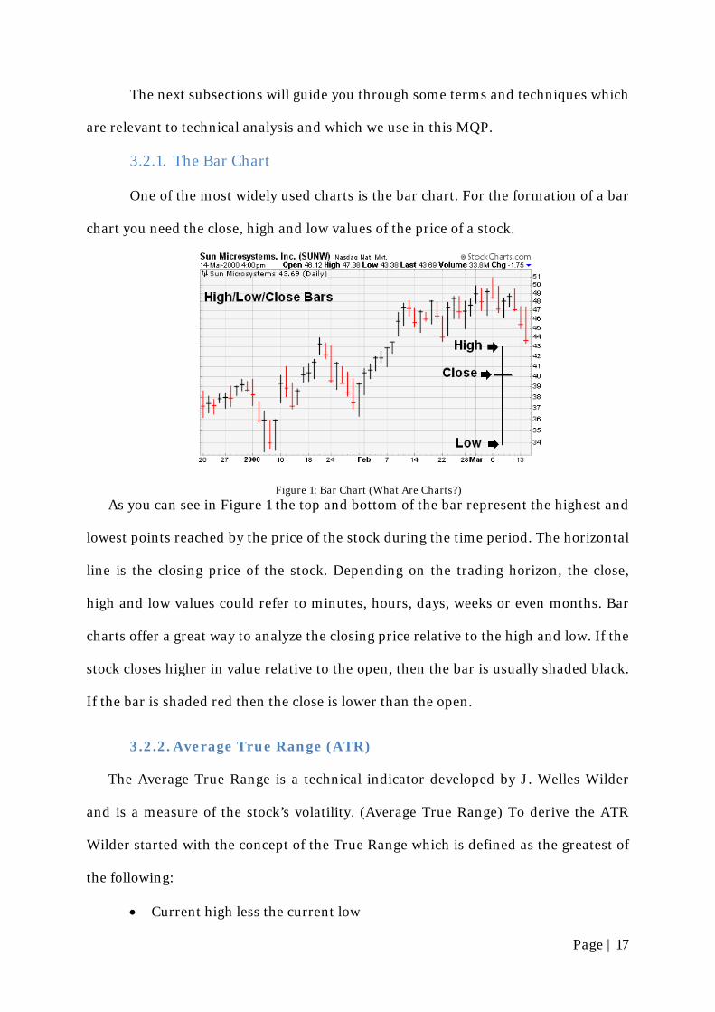
3.2.1. The Bar Chart
One of the most widely used charts is the bar chart. For the formation of a bar
chart you need the close, high and low values of the price of a stock.
Figure 1: Bar Chart (What Are Charts?)
As you can see in Figure 1 the top and bottom of the bar represent the highest and
lowest points reached by the price of the stock during the time period. The horizontal
line is the closing price of the stock. Depending on the trading horizon, the close,
high and low values could refer to minutes, hours, days, weeks or even months. Bar
charts offer a great way to analyze the closing price relative to the high and low. If the
stock closes higher in value relative to the open, then the bar is usually shaded black.
If the bar is shaded red then the close is lower than the open.
3.2.2. Average True Range (ATR)
The Average True Range is a technical indicator developed by J. Welles Wilder
and is a measure of the stock’s volatility. (Average True Range) To derive the ATR
Wilder started with the concept of the True Range which is defined as the greatest of
the following:
• Current high less the current low
Page | 17

• The absolute value of the current high less the previous close
• The absolute value of the current low less the previous close
The ATR is simply the moving average of the True Range over a specified time
period. For example, a more volatile stock will have a higher ATR (e.g., ATR of 4)
than a stock experiencing lower level of volatility (e.g., ATR of 2).
3.3. CAN SLIM
CAN SLIM is a formula created by William J. O'Neil and represents a growth
stock investment strategy that combines fundamental and technical analysis. Bill
O’Neil is the founder of the Investor's Business Daily (IBD), author of the book “How
to Make Money in Stocks” and a highly successful trader whose approach helps both
individual and institutional investors improve their returns. CAN SLIM is a checklist
for seven common characteristics all great performing stocks have before their major
price increase. In the next subsections we will walk you through each part of the CAN
SLIM stock selection process.
3.3.1. C: Current Earnings Growth
The first and foremost indicator of a stock’s performance has been shown by
IBD’s research to be the current earnings growth of the company. The “C” rule says
that stocks must show a major percentage increase in their current quarterly
earnings per share when compared to the same quarter one year ago. The general
rule of thumb is the higher the EPS growth, the better. However, those increases
should be at least 25% and, preferably, they should be accelerating in at least the
three most recent quarters.
Page | 18

3.3.2. A: Annual Earnings Growth
In addition to the strong quarterly earnings results a stock should also show a
major and consistent increase in its annual earnings growth for the past three years.
A CAN SLIM stock should exhibit at least a 25% increase in its annual earnings per
share in each of the last three years. It is considered an even better indication if the
return on equity is higher than 17%.
3.3.3. N: New Products, New Services, New Management, New
Price Highs
IBD’s research shows that all great performing stocks are characterized by a novel
event that triggers the major increase in their stock prices. Often that could be a
shakeup at the top management level that will change the strategic path the company
pursues. This could also be a pioneering product or service that increases the
company’s market share and improves its competitive advantage. O’Neil’s
investment strategy views the price of each stock as its quality measure. Thus, stocks
reaching new highs have proven their quality and have the best potential to continue
climbing up.
3.3.4. S: Supply and Demand
Successful investors understand that any major price movement is subject to the
interactions between the market players. Thus, if the demand for a stock is greater
than the supply of it, the stock price increases. IBD recommends that investors watch
closely the trading volume of the stock as a major change in volume signals that
institutional investors are buying or selling. As a stock begins its rising price
movement CAN SLIM investors should look for a volume change of at least 50%
when compared to the average trading volume over the last 50 days. Similarly, they
Page | 19

should stay alert of any new highs made on a weaker volume, or any new lows made
on higher volume indicating institutional selling.
3.3.5. L: Leader or Laggard
IBD’s research shows that 37% of a stock's move is directly tied to the
performance of the industry the stock is in, and another 12% is due to strength in its
overall sector. To find the best stocks investors should look into the top 22% of
industry groups. Within those industry groups they should further focus on the
leading stocks based on their fundamentals, price movements and market activity.
One way to distinguish the end of a bearish market and confirm a new bullish market
rally is to see emerging leaders making new highs.
3.3.6. I: Institutional Sponsorship
Institutions such as mutual funds and pension funds are the major market
players and only they are capable of propelling a stock to a new high. Because of their
enormous power in the marketplace due to their immense holdings investors should
keep a close eye on the stocks under their belts. A stock candidate for a major price
increase should be owned by at least several institutional sponsors. As a rule of
thumb investors should also look for an increasing number of first-class money
managers who are accumulating the stock.
3.3.7. M: Market
The market direction is deemed as the most critical indicator for investing by
IBD. Studies show that most stocks make their major price gains when the overall
market is bullish. 75% of all stocks also tend to move in the same direction as the
market – either up or down. In order to gauge the market direction investors should
follow closely the market indexes (DJIA, S&P 500, NYSE Composite) and look for
Page | 20

movements signaling market tops or bottoms. An indication of a new uptrend is an
attempt at a rally in one of the indexes which then must follow through the fourth to
tenth day of the rally with another strong day – a major price advance supported by
rising total market volume.
3.3.8. Our CAN SLIM Stock Selection
The backbone of this MQP are the CAN SLIM stocks with their unique
fundamental characteristics and price movements. At the beginning of the project we
decided to back test all CAN SLIM stocks for the past five years. However, due to
software and data crunching limitations imposed by TradeStation we decided to
focus on the CAN SLIM stocks for 2007.
In order to back-test all the CAN SLIM stocks from January 1st, 2007 to January
1st, 2008 we created an indicator for the RadarScreen tool within TradeStation which
allows us to scan all the NYSE and NASDAQ stocks. A stock needs to meet the
following criteria to qualify as a CAN SLIM stock and, thus, suitable for our back-
testing:
• Be listed on the NYSE and NASDAQ exchanges
• Have a minimum stock price of $15
• Have at least two quarters in the last year with EPS growth of at least 25%
• Have annual EPS growth for the last two years of more than 20%
• Have ROE greater than 17
We acknowledge that these criteria do not meet the whole checklist of CAN SLIM
requirements. However, we do believe that they represent the most critical points of
Page | 21

the CAN SLIM investment strategy and the conclusions from our research are by no
means affected by them.
The TradeStation indicator came up with 204 NASDAQ and 358 NYSE stocks
that met all the above criteria during that period (See Appendix 11.6). However, when
we started testing the trading strategies on them, 3 stocks had to be removed from
the list due to data retrieval error, leaving us with a total of 559 CAN SLIM stocks.
3.4. TradeStation
TradeStation is a trading platform which allows for the formulation of strategies,
their back-testing using historical data and automation execution of trades in real-
time. (TradeStation About) It is technical analysis software package which uses a
built-in proprietary programming language called EasyLanguage to develop
numerous technical indicators and strategies. In addition to being a valuable
research and testing tool, TradeStation can complete trades with TradeStation
Securities acting as the broker.
3.5. Performance Measurements
3.5.1. Expectunity and System Quality Measurement
Expectunity is a system developed by Van K. Tharp, Ph.D. which conceptualizes
the amount one should expect to make on average over many trades per dollar
risked. Tharp combines a very simple probability notion, expected value, with
technical analysis and psychological concepts to provide traders with quantitative
measurements of risk and expected profit (Tharp, 2006).
Below we explain the terminology created and utilized by Van Tharp.
Page | 22
Expectancy: It is simply a combination of the winning/losing probability and the
winning/losing payoff of a method.
Opportunity: The frequency at which you will be able to apply your system to
obtain its expectation. In other words, it is the number of trades a system will make
in a particular unit of time (e.g., a year).
Risk: It is defined as the initial entry price of a stock minus the exit price of the
stock that will be realized if the trade moves in a direction opposite of what was
predicted (1R). This exit point is designed to help traders protect their capital. If a
stock is bought at $50, and the trader decides to sell if it drops to $48, the initial risk
is $2 per share; hence 1R is equal to $2.
R-Multiples: A trade’s reward/risk ratio. To calculate a trade’s R-multiple, divide
the number of points captured at the exit of the position by the initial risk.
Expectunity: It is a combination of expectation and opportunity. This
combination determines the worth of any trading system or method. Multiplying the
expectancy times the opportunity factor provides the concept of expectunity.
Van Tharp’s expectunity methodology was later revised and improved by Michael
J. Radzicki, Ph.D, Worcester Polytechnic Institute. By adjusting the expectunity with
the standard deviation of R-Multiples amongst all trades performed, he created the
Systems Quality concept. This concept accounted for the volatility between the
trades, providing a fair comparison ground amongst a wide range of strategies.
3.5.2. Monte Carlo Analysis
The Monte Carlo method is a computational technique which generates results
based on repeated random sampling. The term “Monte Carlo” is a reference to the
famous casino “Monte Carlo” in Monaco where one of the method’s founders’ uncle
would borrow money to gamble. The use of randomness and the repetitive nature of
Page | 23
the process are analogous to the gambling activities happening in the casino.
(Investopedia)
Monte Carlo simulation is a method that helps reduce the uncertainty involved in
estimating future outcomes. Monte Carlo’s characteristics make it useful for
applications to complex, non-linear models or in the performance measurement of
other models. With Monte Carlo analysis the researcher can estimate the probability
of certain outcomes by simulation multiple times using random variables.
When the Monte Carlo technique is used to simulate trading, samples from the
list of trades are generated to form a trading sequence. Then, each trading sequence
is analyzed, and the results are sorted to determine the probability of each result,
with each being assigned a confidence level. With Monte Carlo a trader can
determine that, after thousands of different sequences of trades had been analyzed,
his return on equity ratio might be 19% with 95% confidence, or in 95% of all cases.
Thus, Monte Carlo allows the trader to see what could have happened if the trading
sequence was randomized and the ROE calculated for each one of them. (Bryant)
In our MQP the performance measurements we focus on by using Monte Carlo
are profit factor, worst case drawdown and the return to drawdown ratio. The first
one is calculated by gross profit by gross loss. It can also be interpreted as the
number of dollars made for every dollar lost.
Drawdown is defined as a percentage retracement in equity from a peak to trough
prior to a new equity high being made. The worst case drawdown measures the
amount of money required to survive the largest equity dip during the back-testing
period. Drawdowns can be easily spotted in equity curves graphs which show the
value of a trading account graphed over a period of time. A drawdown is identified
by looking from the highest peaks to the lowest peaks moving forward. The return on
drawdown ratio determines which strategy has the highest returns while enduring
Page | 24
the least amount of volatility. A higher ratio is generally better because it means that
the strategy receives a higher return relative to risk.
4. Complete Trading Strategies
In the opening paragraph we stated that along with the important contributions
this MQP makes to the academic research on trading, we also target individual
investors who are willing to challenge their principles to achieve higher returns and
peace of mind. We believe that the only way to consistently compare different
approaches of trading CAN SLIM stocks is to develop complete trading strategies.
The characteristics and principles embedded in a complete trading strategy allow for
the collection and analysis of measurable data and their interpretation to form
conclusive suggestions to our audience as to how to invest in CAN SLIM stocks.
Complete trading strategies provide us with insight into many areas but more
importantly they do not allow us to confuse ourselves and limit our performance by
making decisions we are neither intellectually nor psychologically capable of doing.
Many people believe that trading is all about predicting where the market is going
and being right all the time. In reality, the market is comprised of thousands of
individuals taking positions every second so it is delusional, useless and expensive to
think that you can time its direction or understand its workings. An obvious question
arises: “If I cannot predict the market, does that mean I cannot outperform it and I
should simply invest in a mutual fund getting the average return of S&P 500?” The
answer is short: No. A guru of trading Charlie Wright, whose book “Trading as a
Business” we refer to numerous times in this MQP, argues that successful traders
make money because they do not predict the market but rather trade it correctly. The
latter is achieved by following sound trading rules which have nothing to do with
predicting the market. (Wright, 1998)
Page | 25
In order to be profitable in the long-run trading requires a disciplined approach
to developing a complete trading strategy by following proper trading principles. In
our MQP these take the form of five steps:
1. Set-up: Decide under what conditions you will enter the market
2. Entry: Decide how exactly you will enter the market
3. Exit with a profit: Decide how to exit the market and take your profits
4. Exit with a loss (Money Management Stop): Decide how much you are willing
to lose at each trade
5. Cash Management: Decide how much of your capital to allocate to each
position
Due to the complexity of creating an algorithm for implementing money
management using TradeStation, we do not use this aspect of the complete trading
strategy in our MQP. We focus on comparing the set-up while keeping the entry, the
exit with a profit and the money management stops constant. In the next five
subsections we will walk you through the details of each one of these rules for
successful trading.
4.1. Set-up
The set-up is a condition or a set of conditions which are required to hold true
before considering taking a position in the market. The set-up does not get you in the
market, it is not used to purchase or sell a position. Examples of set-ups include:
• A longer moving average crossing above a shorter moving average
• Price moving above a moving average
• Price being at the highest high of a certain time period
Page | 26

Charlie Wright argues that any indicator could be used as the set-up in a
profitable strategy. There can be an infinite number of set-ups as they are limited
only by your imagination. The set-up only prepares you to get you in the market; it
neither gets you long or short nor does it determine your profits or losses. It is the
interaction between the set-up and the entry that makes your strategy more precise
in executing its trades, and, ultimately, more profitable. (Wright, 1998)
4.2. Entry
Once the set-up rules have been met, the signal by which the strategy gets you in
the market is called the entry. There are two rules to which an entry should adhere:
1. The direction of the price should follow the direction expected by the set-up
2. The entry should be designed to capture all the price movements it was
intended for
The first rule states that if the set-up alerts you that a long position is being made,
the direction of the price should confirm it, that is, go up. Thus, our entry confirms
the buy signal given by the set-up and only then gets us in the market.
The second rule makes sure that our entry catches all of the price movements that
it was designed for. This rule will be violated if, for example, the entry misses a big
price move. Thus, the entry used must be customized to meet the specifics of your
strategy.
Examples of buy entries are:
• A buy stop order above the current bar’s high
• Buy at market after a close over the previous bar’s high
The first example uses a stop order which states that if the market should move
above a certain specified price you are stopped into a position. The second example
Page | 27
gets you at the market determined price but only if the close is higher than the
previous bar’s high.
4.3. Exit with a profit
In this MQP we use the concept of a set-up and entry to take a position in the
market. In order to take profits at a predetermined price level, or based on certain
market conditions, various exit strategies can be used. These are used with a profit
objective and are not targeted at protecting your initial capital. The latter is achieved
by your money management stops, which we will talk about more in the next
subsection. Exits with a profit are based on certain market activity and should be
used only to get you out of the market if specific market conditions are met.
Examples of exits with a profit are:
• A tightening exit which gets you (say) 50% out of your position when profits
reach 50%, then another 25% when profits reach 75% and the rest 25% when
profits reach 100%
• A trailing Average True Range hanging from the highest point after the entry
date
In the first example the strategy exits the position and takes profits at
predetermined profit levels. In the second example the strategy generates an order to
exit the position at the highest price since the entry of the trade less the ATR value.
This stop value moves up (trails) as the trade progresses. The second example is the
actual exit with a profit that we use in our MQP and it stays constant across all tests.
Page | 28

4.4. Exit with a loss (Money management stop)
Money management stops are used for only one purpose – to protect your initial
equity. They represent the maximum amount the trader is willing to risk at the
beginning of the trade. Usually, the money management stops are a simple dollar
figure or a percent of the capital. However, to account for the volatility across
financial instruments they can also be based on technical indicators such as the ATR.
For example, a money management stop exits the position if the stock reaches a
calculated using the ATR dollar amount below the current bar's closing price. This
order is only used for the bar of entry to protect against an initial reversal.
4.5. Money Management
A complete trading strategy is finalized by the concept of money management
which deals with position sizing and risk control. This technique determines how
much of your equity you allocate to each trade and how you diversify your portfolio
amongst various investment instruments. The size of the trade and the subsequent
addition to it at the right time are crucial for the development of a successful and
profitable strategy. For example, skilled traders manage their money to benefit from
the market moves. They pyramid up when the market moves in their favor and use
their accumulated profits to add to their position without risking their initial capital.
This is the most intricate part of a complete trading strategy and is deemed by many
as the one that can give you a market edge. Due to the same reason, it is also very
complicated one to code and requires extensive back-testing.
Page | 29

5. Back-Testing using TradeStation
5.1. Overview of the Back-Testing Procedure
Back-testing is an integral part of developing an effective trading strategy. In
back-testing traders apply their strategies to historical data and check how they
would have performed in those past market conditions. The results obtained can be
studied to evaluate the strategy’s efficiency and performance. Traders can also
optimize their strategies, determine the flaws, and gain confidence in their strategy
before applying it to the real markets.
Back-testing assumes that a system’s past statistical character is a good indicator
of its future statistical character, hence any strategy that worked well in the past is
likely to work well in the future, and conversely, any strategy that performed poorly
in the past is likely to perform poorly in the future. In order not to be misguided by
back-testing results, it is advisable to test the strategy across various time frames and
under different market conditions. Even though a strategy yields positive results in a
bull market, the results might be completely different in a bear or a sideways market.
It is often a good idea to back-test over a long time frame that encompasses several
different types of market conditions.
As mentioned before, we chose to trade the 559 CAN SLIM Stocks of 2007 on a
daily basis. In order to retrieve comparable results for the five set-ups in our back-
testing procedure, we assume ceteris paribus, keeping all the other aspects of a
complete trading strategy constant.
When back-testing the six possible trading strategies we determined, we
alternated our set-up between moving average crossover, Bollinger bands, Keltner
channel, Donchian channel 20-day and 55-day, and volume breakouts.
Page | 30

We chose “Buy stop order one tick above the current bar’s high” as our entry,
which essentially places a buy stop order once the price reaches one tick higher than
what was confirmed by the set-up.
A Trailing Average True Range serves as our exit with a profit, where a 3-ATR
limit was hanging from the highest point in the stock’s price movement. A 3-ATR
resistance was also set to the price of the stock at the day of entry, which was geared
towards protecting our initial capital from a potential wrong buy signal. In order to
effectively utilize the back-testing results we retrieve, all the open positions are
closed on the last trading day of 2007. The strategies we apply in TradeStation also
require data since October 18th, 2006, however, the period in which we start trading
is January 1st, 2007.
5.2. Moving Average Crossover
The moving average is a trend following indicator that is commonly used in
technical analysis. It shows the average value of a stock's price over a pre-determined
time period. By smoothening data series, it makes it easier to recognize trends,
measure momentum and define areas of possible support and resistance. Two
arithmetic averages of the same asset price are calculated based on two length inputs
specified by traders.
The most common utilization of moving averages it to build a trading strategy
based on moving average crossovers. This strategy will use two moving averages,
and will provide a buy signal when the short-term average advances above the long-
term average.
An upward trend is said to occur when a short-term average crosses above a
longer-term average, yielding a buy signal. Similarly, a downward trend said to occur
Page | 31

when a short-term average crosses below a long-term average, resulting in a sell or
sell-short signal.
In our MQP we look at the intersection of two moving averages, a 9-day and an
18-day. When the 9-day moving average crosses over the 18-day moving average, we
interpret is as a buy signal. Conversely, a sell signal is interpreted when the reverse
crossover occurs.
5.3. Bollinger Bands
Developed by John Bollinger, Bollinger bands are an indicator that allows traders
to compare volatility and relative price levels over a period time. It is a technique that
uses moving averages with two trading bands and simply adds and subtracts a
standard deviation calculation from the moving average. Many traders use them
primarily to determine overbought and oversold levels. The indicator consists of
three bands designed to cover the majority of a stock's behavior:
1. A simple moving average in the middle
2. An upper band (Simple moving average plus 2 standard deviations)
3. A lower band (Simple moving average minus 2 standard deviations)
Standard deviation is a mathematical formula that measures volatility, showing
how the stock price can be spread around its actual value. Sharp price increases or
decreases, and hence volatility, will lead to a widening and, respectively, contracting
of the bands. At times of low volatility, when the bands are tightened, Bollinger
Bands do not give any hints of a stock’s behavior. Bollinger recommends using a 20-
day simple moving average for the center band and 2 standard deviations for the
outer bands.
Page | 32

Alone, Bollinger bands serve two primary functions: identify periods of high and
low volatility and recognize when prices are at extreme, and possibly unsustainable,
levels. Although these functions indicate buy or sell signals, the pattern is not geared
towards determining the price behavior of a stock. Other technical analysis tools are
recommended to help determine the direction of a potential breakout.
When using this chart pattern, bands are designated as price targets. If the price
deflects off the lower band and crosses above the 20-day simple moving average the
upper band comes to represent the upper price target. In a strong uptrend, prices
usually fluctuate between the upper band and the 20-day simple moving average. In
such a trend, crossing below the 20-day simple moving average initiates a sell signal.
When the stock price recurrently strikes the upper Bollinger Band, the price is
thought to be overbought. Likewise, when the price strikes the lower band, it is
thought to be oversold, and a buy signal would kick in.
5.4. Keltner Channel
Chester W. Keltner introduced and developed the Keltner Channels in his book
"How to Make Money in Commodities" (Staff). Simply, Keltner Channels are three
moving average bands:
1. The middle line represents the moving average of the closing price of the
asset
2. The upper channel represents the average of the high asset price,
calculated over a 10-day period ( 1.5 Average True Ranges above the
moving average)
3. The lower channel represents the average of the low asset price calculated
over a 10-day period ( 1.5 Average True Ranges below the moving average)
Page | 33

When the stock price is approaching the lower channel the market is considered
oversold, which should indicate a buy signal to traders. Similarly, when the stock
price is closer to the upper channel the market is considered overbought, indicating a
sell signal.
5.5. Volume Breakout
The volume of an asset represents the number of shares or contracts traded in the
market during a given period of time, as a measure of activity. In technical analysis,
the volume indicator serves a heavy role in determining the worth of a market move.
A higher volume increases the significance of any price movements. Trading activity
also relates to the liquidity of a stock, so a higher volume also indicates that the
security can be easily traded.
The volume breakout strategy plots current daily trading volume of the security
against the 10-day average daily volume. In our MQP, a buy signal is interpreted
when the former exceeds the latter by at least 50%, as suggested by William O’Neal’s
CAN SLIM methodology.
5.6. Donchian Channel 20-Day and 55-Day
Donchian channels are price channels designed to work well with trend-following
systems. This simple breakout system is developed by Richard Donchian, considered
to be the father of successful trend following (Lee). It plots the highest high and
lowest low over the last X time period intervals. The signals derived from this system
are based on the following basic rules:
• Buy/ Buy to cover when prices penetrate and close above the upper channel
• Sell/Sell short when prices penetrate and close below the lower channel
Page | 34

The Donchian channel strategy aims at initiating a position at the beginning of a
new trend through the penetration of either the upper or the lower channel. The
theory behind this study states that if the current price manages to exceed the range's
high propped up by enough momentum, then a new high, signaling an uptrend, will
be established. Conversely, price crossing below the range's low indicates a new
downtrend.
In our MQP we test two time intervals using the Donchian channels – a 20-day
and a 55-day time period. The shorter-term system is expected to generate more
trades but also to catch the breakouts earlier while the longer-term system is
expected to be “smoother” – have less trades but with a higher percentage of
winners.
Page | 35

6. Results Attained from Back-testing
In this section we exhibit the results of our back-testing for the different
strategies. At first we present the settings for each strategy then we provide screen
shots to only three of the stocks we tested; AAPL: Apple Inc. (NASDAQ), MTL:
Mechel OAO (NYSE) and RIMM: Research in Motion Limited (NASDAQ). However,
we only provide explanatory comments about the performance of each strategy on
AAPL to avoid repetitive remarks. We also present the results for each strategy
based on the Monte Carlo simulation and the system quality calculations which we
discuss in Section 7.
6.1. Bollinger Bands
6.1.1. TradeStation Settings
TradeStationChart Settings
Interval Daily Start Date/Time 10/18/2006 16:00 End Date/Time 1/2/2008 16:00
TradeStation Strategies Applied BBands+ATR(On) TradeStation Strategy Inputs
Description Value BBands+ATR – Bollinger Price Close BBands+ATR – Test Price Long Band Close
BBands+ATR – Days Back 20 BBands+ATR – No. of Standard Deviation 2 BBands+ATR – ATR Days Back 10
BBands+ATR – No. of ATRs 3 BBands+ATR – Initial Stop ATRs 5 BBands+ATR – Initial Stop ATR Days Back 2
TradeStation Strategy Settings Initial Capital $100.00 Commission (per Trade) $0.00
Slippage (per Trade) $0.00 Interest Rate 0.00%
Table 1 - TradeStation Settings for Bollinger Bands
Page | 36

6.1.2. AAPL: Apple Inc. (NASDAQ)
Figure 2- Trades Generated by Bollinger Bands, AAPL
The above figure shows the performance of the Bollinger bands strategy over the
trading period. The blue line is the upper Bollinger band, the gray line is the moving
average and the red line is the lower Bollinger band. The “BuyBBand” label shows
when the strategy takes a long position and the label “Exit” is our exit with a profit
based on an ATR value. The Bollinger bands capture only the uptrend starting in late
August and miss the big move from the beginning of 2007. The exit also gets us
prematurely out of the position. Overall, as we will later see from the performance
measures, this strategy does not work well with CAN SLIM stocks.
Page | 37

6.1.3. MTL: Mechel OAO (NYSE)
Figure 3 - Trades Generated by Bollinger Bands, MTL
6.1.4. RIMM: Research in Motion Limited (NASDAQ)
Figure 4 - Trades Generated by Bollinger Bands, RIMM
Page | 38

6.1.5. Equity Curve
Figure 5 - Equity Curve Generated by Bollinger Bands
The Bollinger bands strategy generated 2749 trades for the 559 CAN SLIM stocks.
The above equity curve based on all these trades shows the status of the trading
account throughout the trading period. It can be observed that the Bollinger bands
subjects the trader to huge drawdowns. Thus, the trader needs to be able to
psychologically endure the pain associated with such losses in equity in order to
trade this strategy.
Page | 39

6.1.6. Monte Carlo Simulation Results at a 95% Confidence
Figure 6 - Monte Carlo Results of Bollinger Bands at a 95% Confidence
6.1.7. Raw System Quality Results
Complete Statistics
Sum of R 332.5405554Number of Trades 2478Expected Value 0.386198547Expectancy 0.134197157Expectunity 332.5405554Std Dev R 2.805904487E / StdDev 0.047826702Study Days 365Opportunities 2478System Quality 118.514567
Percentage of Winning Trades 0.407990315Percentage of Losing Trades 0.591606134Average Winning Trade 5.119604352Average Losing Trade 2.877844475
Table 2- System Quality Results for Bollinger Bands
Page | 40

6.2. Volume Breakout
6.2.1. TradeStation Settings
TradeStationChart Settings Interval Daily Start Date/Time 10/18/2006 16:00 End Date/Time 1/2/2008 16:00
TradeStation Strategies Applied
Volume + ATR + MMS(On)
TradeStation Strategy Inputs Description Value Volume + ATR + MMS ‐ ATR Days Back 10 Volume + ATR + MMS – No. of ATRs 3 Volume + ATR + MMS – Initial Stop ATRs 10 Volume + ATR + MMS – Initial Stop ATR Days Back 3 Volume + ATR + MMS – Holding Period 5 Volume + ATR + MMS – Avg. Days Back 10 Volume + ATR + MMS – Breakout Percentage 50
TradeStation Strategy Settings Initial Capital $100.00 Commission (per Trade) $0.00 Slippage (per Trade) $0.00 Interest Rate 0.00%
Table 3 - TradeStation Settings for Volume Breakout
Page | 41

6.2.2. AAPL: Apple Inc. (NASDAQ)
Figure 7 - Trades Generated by Volume Breakout, AAPL
The above figure shows the performance of the volume breakouts strategy on
AAPL. The red bars on the bottom of the graph represent the volume activity for that
day. You can see that the “BuyVolBrkout” labels correlate highly with the spikes in
their respective volume bars. This strategy generates a lot of trades and catches
almost all of the uptrend.
Page | 42
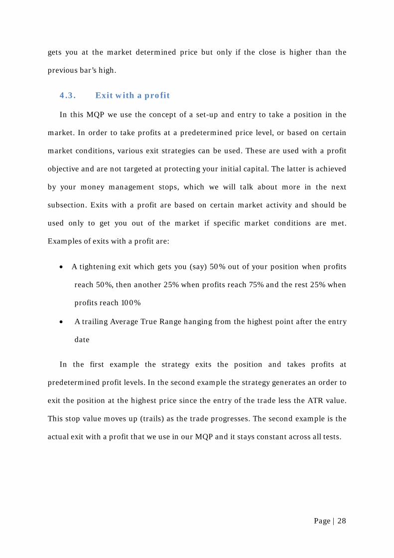
6.2.3. MTL: Mechel OAO (NYSE)
Figure 8 - Trades Generated by Volume Breakout, MTL
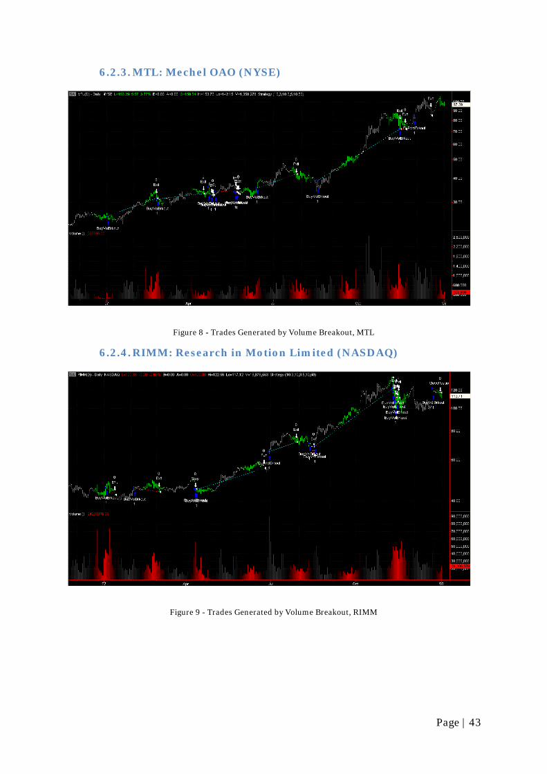
6.2.4. RIMM: Research in Motion Limited (NASDAQ)
Figure 9 - Trades Generated by Volume Breakout, RIMM
Page | 43
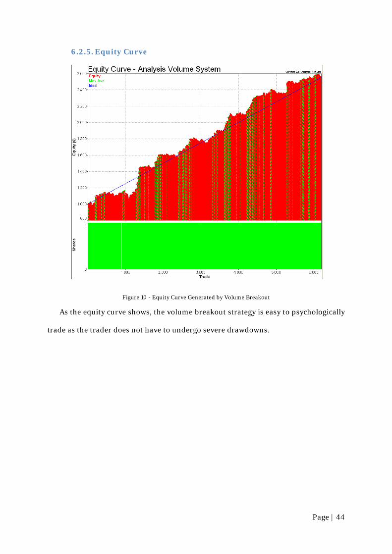
6.2.5. Equity Curve
Figure 10 - Equity Curve Generated by Volume Breakout
As the equity curve shows, the volume breakout strategy is easy to psychologically
trade as the trader does not have to undergo severe drawdowns.
Page | 44
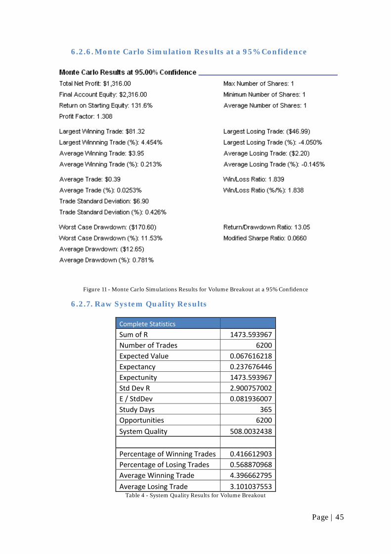
6.2.6. Monte Carlo Simulation Results at a 95% Confidence
Figure 11 - Monte Carlo Simulations Results for Volume Breakout at a 95% Confidence
6.2.7. Raw System Quality Results
Complete Statistics
Sum of R 1473.593967Number of Trades 6200Expected Value 0.067616218Expectancy 0.237676446Expectunity 1473.593967Std Dev R 2.900757002E / StdDev 0.081936007Study Days 365Opportunities 6200System Quality 508.0032438
Percentage of Winning Trades 0.416612903Percentage of Losing Trades 0.568870968Average Winning Trade 4.396662795Average Losing Trade 3.101037553
Table 4 - System Quality Results for Volume Breakout
Page | 45
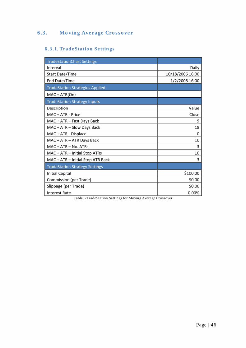
6.3. Moving Average Crossover
6.3.1. TradeStation Settings
TradeStationChart Settings Interval Daily Start Date/Time 10/18/2006 16:00
End Date/Time 1/2/2008 16:00
TradeStation Strategies Applied
MAC + ATR(On)
TradeStation Strategy Inputs
Description Value MAC + ATR ‐ Price Close MAC + ATR – Fast Days Back 9 MAC + ATR – Slow Days Back 18 MAC + ATR ‐ Displace 0 MAC + ATR – ATR Days Back 10 MAC + ATR – No. ATRs 3 MAC + ATR – Initial Stop ATRs 10
MAC + ATR – Initial Stop ATR Back 3
TradeStation Strategy Settings
Initial Capital $100.00 Commission (per Trade) $0.00 Slippage (per Trade) $0.00
Interest Rate 0.00% Table 5 TradeStation Settings for Moving Average Crossover
Page | 46

6.3.2. AAPL: Apple Inc. (NASDAQ)
Figure 12 - Trades Generated by Moving Average Crossover, AAPL
The above graph shows the performance of the moving average crossover strategy
on AAPL. The cyan line represents the fast moving average and the purple line
represents the slow moving average. The strategy does not enter the market on every
crossover due to the limitations imposed by the entry.
Page | 47
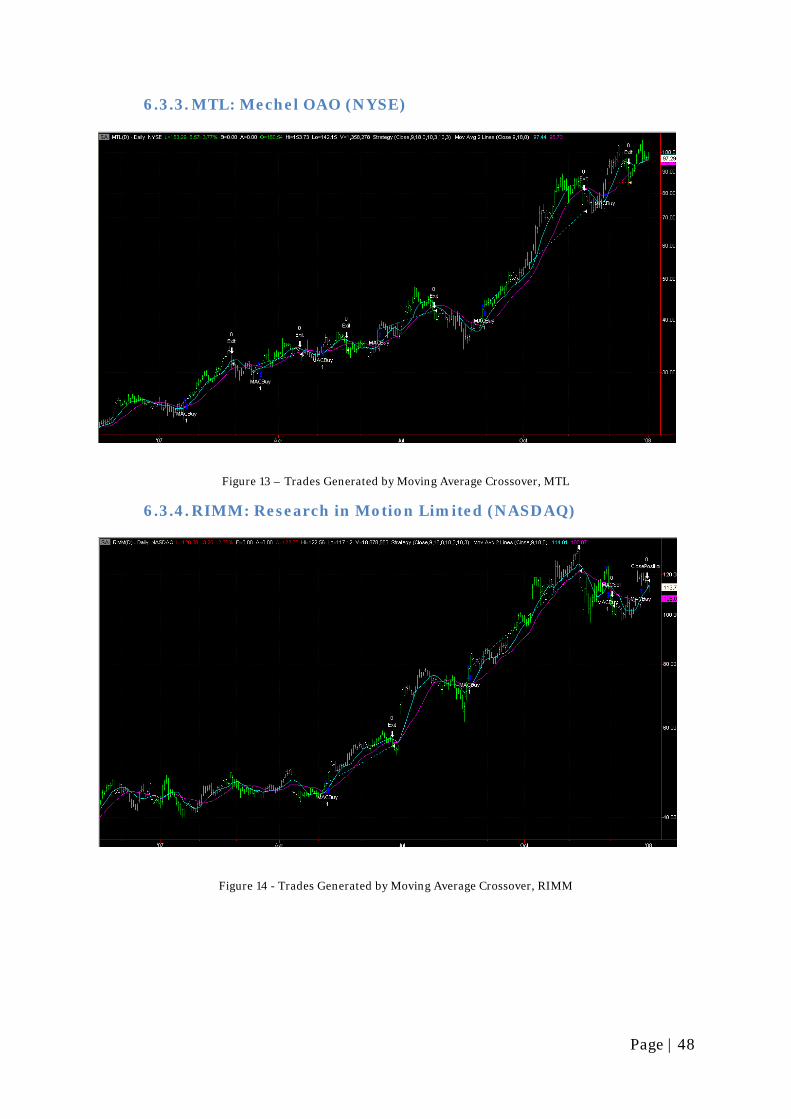
6.3.3. MTL: Mechel OAO (NYSE)
Figure 13 – Trades Generated by Moving Average Crossover, MTL
6.3.4. RIMM: Research in Motion Limited (NASDAQ)
Figure 14 - Trades Generated by Moving Average Crossover, RIMM
Page | 48

6.3.5. Equity Curve
Figure 15 - Equity Curve Generated by Moving Average Crossover
The moving average crossover strategy generates 3414 trades throughout 2007,
with an expected profit of $0.74 per trade. Traders who choose this strategy will
experience a profit of 252%, however the equity curve shows us that this will not
happen uniformly.
Page | 49

6.3.6. Monte Carlo Simulation Results at a 95% Confidence
Figure 16 - Monte Carlo Simulation Results for Moving Average Crossover at a 95% Confidence
6.3.7. Raw System Quality Results
Complete Statistics Sum R 1361.049776 Number of Trades 3414 Expected Value 0.737955477 Expectancy 0.398667187 Expectunity 1361.049776 Std Dev R 3.667327188 E / StdDev 0.108707832 Study Days 365 Opportunities 3414 System Quality 371.1285375 Percent Winning Trades 0.392501465 Percent Losing Trades 0.601640305 Average Winning Trade 4.7175 Average Losing Trade 1.851056475 Table 6 - System Quality Results for Moving Average Crossover
Page | 50
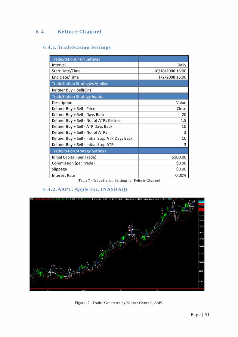
6.4. Keltner Channel
6.4.1. TradeStation Settings
TradeStationChart Settings Interval Daily Start Date/Time 10/18/2006 16:00 End Date/Time 1/2/2008 16:00
TradeStation Strategies Applied
Keltner Buy + Sell(On)
TradeStation Strategy Inputs Description Value Keltner Buy + Sell ‐ Price Close Keltner Buy + Sell ‐ Days Back 20 Keltner Buy + Sell ‐ No. of ATRs Keltner 1.5 Keltner Buy + Sell ‐ ATR Days Back 10 Keltner Buy + Sell ‐ No. of ATRs 3 Keltner Buy + Sell ‐ Initial Stop ATR Days Back 10 Keltner Buy + Sell ‐ Initial Stop ATRs 3
TradeStation Strategy Settings Initial Capital (per Trade) $100.00 Commission (per Trade) $0.00 Slippage $0.00 Interest Rate 0.00%
Table 7 - TradeStation Settings for Keltner Channel
6.4.2. AAPL: Apple Inc. (NASDAQ)
Figure 17 - Trades Generated by Keltner Channel, AAPL
Page | 51

The above figure shows the performance of the Keltner Channel strategy over the
trading period. The blue line is the upper Keltner Channel, the gray line is the
moving average and the red line is the lower Keltner Channel. The “KeltnerBuy”
labels indicate when traders should take a long position in the market, whereas the
“Exit” labels where the Keltners indicate a yield signal. Although the Keltner Channel
strategy generates quite a few trades, we cannot exactly call it a successful strategy
since it misses the majority of the breakouts. We receive false buy signals, but our
exits are agile enough to get us out of the trade with minimum losses.
6.4.3. MTL: Mechel OAO (NYSE)
Figure 18 - Trades Generated by Keltner Channel, MTL
Page | 52

6.4.4. RIMM: Research in Motion Limited (NASDAQ)
Figure 19 - Trades Generated by Keltner Channel, RIMM
6.4.5. Equity Curve
Figure 20 - Equity Curve Generated by Keltner Channel
Page | 53

The equity curve proves us that the Keltner Channel Strategy is relatively easy to
trade. The trading account is very close, and mostly above the ideal equity, hence
traders should not worry about large drawdowns in their account.
6.4.6. Monte Carlo Simulation Results at a 95% Confidence
Figure 21 - Monte Carlo Simulation Results for Keltner Channel at a 95% Confidence
Page | 54

6.4.7. Raw System Quality Results
Complete Stats
Sum R 615.6322646Number of Trades 2750Expected Value 0.588741818Expectancy 0.223866278Expectunity 615.6322646Std Dev R 2.825176056E / StdDev 0.079239762Study Days 365Opportunities 2750System Quality 217.9093453
Percent Winning Trades 0.444Percent Losing Trades 0.553090909Average Winning Trade 4.602039312Average Losing Trade 2.629881657
Table 8 - System Quality Results for Keltner Channel
6.5. Donchian Channel 20-day
6.5.1. TradeStation Settings
TradeStationChart Settings
Interval Daily Start Date/Time 10/18/2006 16:00
End Date/Time 1/2/2008 16:00
TradeStation Strategies Applied
Donchian Channel(On)
TradeStation Strategy Inputs
Description Value Donchian Channel ‐ Days Back 20 Donchian Channel ‐ ATR Days Back 10 Donchian Channel ‐ No. of ATRs 3 Donchian Channel ‐ Initial Stop ATRs 5
Donchian Channel ‐ Initial Stop ATR Days Back 2
TradeStation Strategy Settings
Initial Capital $100,000.00 Commission (per Trade) $0.00 Slippage (per Trade) $0.00 Interest Rate 2.00%
Page | 55

Back‐testing Resolution Look‐Inside‐Bar Back‐Testing Disabled
MaxBarsBack 60 Table 9 - TradeStation Settings for Donchian Channel 20-day
6.5.2. AAPL: Apple Inc. (NASDAQ)
Figure 22- Trades Generated by Donchian Channel 20-Day, AAPL
The above graph shows the trading performance of the Donchian Channel 20-Day
strategy on Apple. We can clearly see that the strategy catches the two major
breakouts, in March and in late August. The exits are designed well, getting traders
out of the position around the maturity of the breakout. The money management
stops are very agile to react to the false buy signals.
Page | 56

6.5.3. MTL: Mechel OAO (NYSE)
Figure 23 - Trades Generated by Donchian Channel 20-Day, MTL
6.5.4. RIMM: Research in Motion Limited (NASDAQ)
Figure 24 - Trades Generated by Donchian Channel 20-Day, RIMM
Page | 57

6.5.5. Equity Curve
Figure 25 - Equity Curve Generated by Donchian Channel 20-Day
By looking at the Equity Curve we can tell that Donchian Channel 20-Day strategy
does not encompass large drawdowns, hence traders should not worry about losing a
large portion of their account before beginning to profit from the system. However
although the system generates approximately a 110% profit, traders would not
experience these until the last quarter of the trading period.
Page | 58
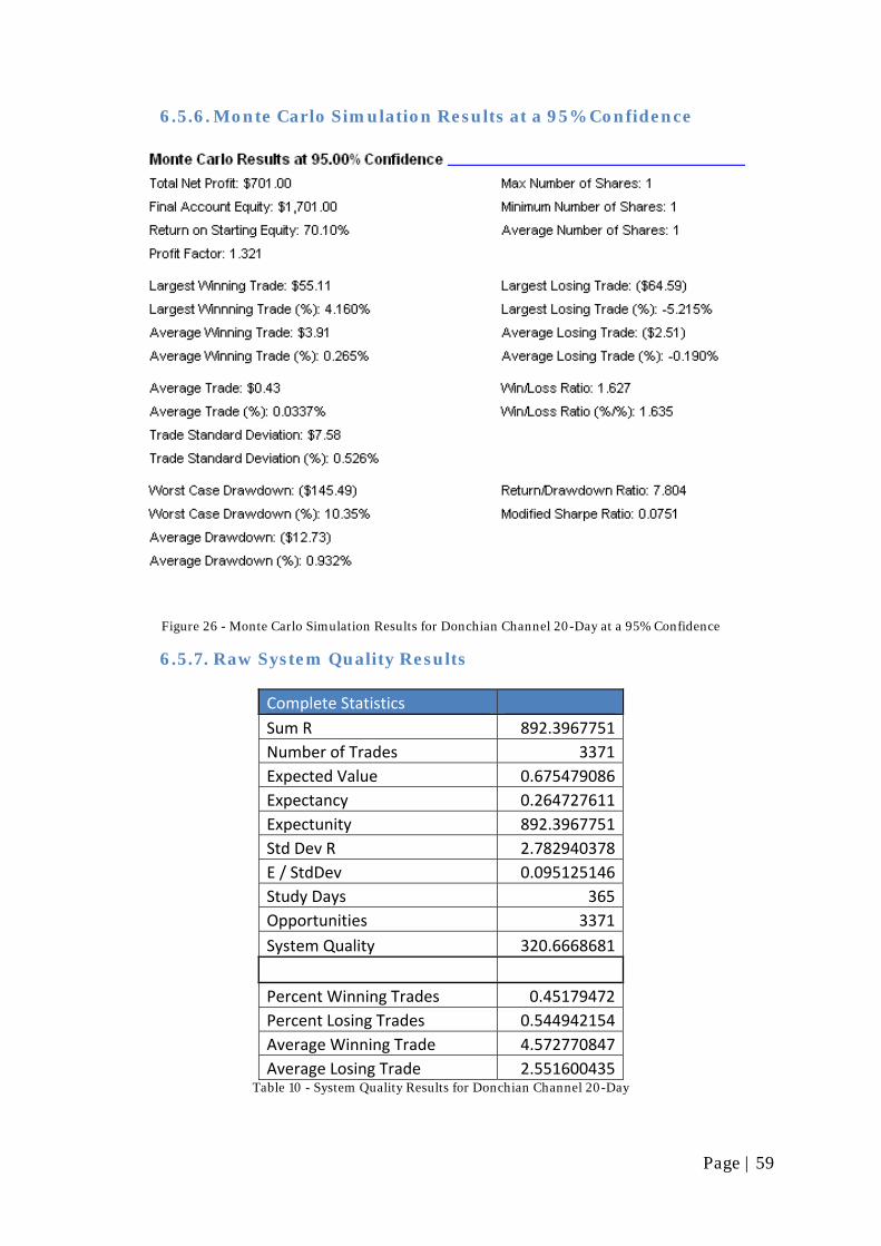
6.5.6. Monte Carlo Simulation Results at a 95% Confidence
Figure 26 - Monte Carlo Simulation Results for Donchian Channel 20-Day at a 95% Confidence
6.5.7. Raw System Quality Results
Complete Statistics Sum R 892.3967751Number of Trades 3371Expected Value 0.675479086Expectancy 0.264727611Expectunity 892.3967751Std Dev R 2.782940378E / StdDev 0.095125146Study Days 365Opportunities 3371System Quality 320.6668681
Percent Winning Trades 0.45179472Percent Losing Trades 0.544942154Average Winning Trade 4.572770847Average Losing Trade 2.551600435
Table 10 - System Quality Results for Donchian Channel 20-Day
Page | 59
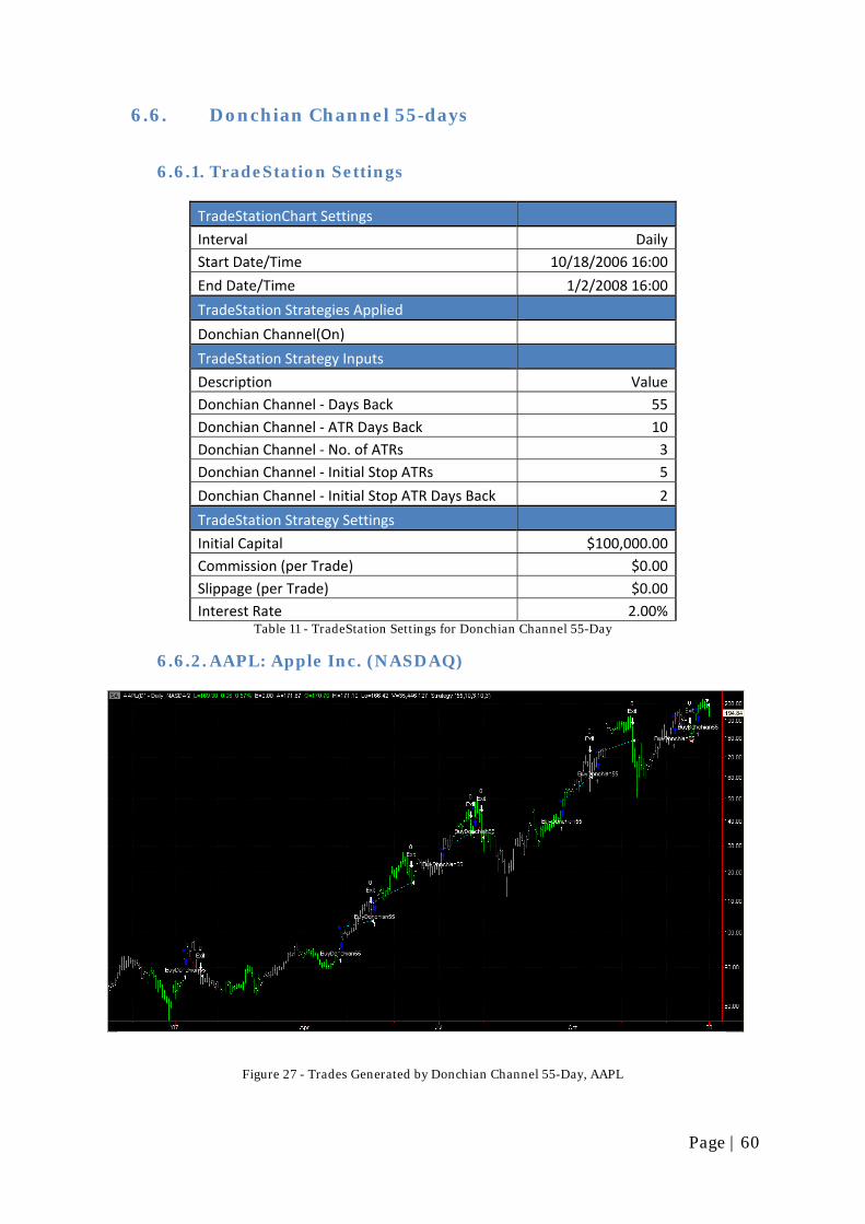
6.6. Donchian Channel 55-days
6.6.1. TradeStation Settings
TradeStationChart Settings
Interval Daily Start Date/Time 10/18/2006 16:00
End Date/Time 1/2/2008 16:00
TradeStation Strategies Applied
Donchian Channel(On)
TradeStation Strategy Inputs
Description Value Donchian Channel ‐ Days Back 55 Donchian Channel ‐ ATR Days Back 10 Donchian Channel ‐ No. of ATRs 3 Donchian Channel ‐ Initial Stop ATRs 5
Donchian Channel ‐ Initial Stop ATR Days Back 2
TradeStation Strategy Settings
Initial Capital $100,000.00 Commission (per Trade) $0.00 Slippage (per Trade) $0.00 Interest Rate 2.00%
Table 11 - TradeStation Settings for Donchian Channel 55-Day
6.6.2. AAPL: Apple Inc. (NASDAQ)
Figure 27 - Trades Generated by Donchian Channel 55-Day, AAPL
Page | 60

The Donchian Channel 55-Day strategy trades effectively throughout the year of
2007. The major breakouts are caught with minor delays; however this strategy has
the least wrong buy signals, minimizing drawdowns.
6.6.3. MTL: Mechel OAO (NYSE)
Figure 28 - Trades Generated by Donchian Channel 55-Day, MTL
6.6.4. RIMM: Research in Motion Limited (NASDAQ)
Figure 29 - Trades Generated by Donchian Channel 55-Day, RIMM
Page | 61

6.6.5. Equity Curve
Figure 30 - Equity Curve Generated by Donchian Channel 55-Day
The equity curve for the Donchian Channel 55-Day Strategy is almost uniform,
and has minimal drawdowns throughout the trading period. Although the strategy
has relatively low returns, it is an easy-to-trade strategy since traders do not have to
withstand big losses.
Page | 62

6.6.6. Monte Carlo Simulation Results at a 95% Confidence
Figure 31 - Monte Carlo Simulation Results for Donchian Channel 55-Day at a 95% Confidence
6.6.7. Raw System Quality Results
Complete Statistics Sum R 522.753486Number of Trades 2364Expected Value 0.58427665Expectancy 0.221130916Expectunity 522.753486Std Dev R 2.657478962E / StdDev 0.083210787Study Days 365Opportunities 2364System Quality 196.7103008
Percent Winning Trades 0.438663283Percent Losing Trades 0.560067682Average Winning Trade 4.705429122Average Losing Trade 2.642220544
Table 12 - System Quality Results for Donchian Channel 55-Day
Page | 63

7. Comparison of the Strategies
7.1. System Quality Comparison
System Quality Comparison
Moving Average
Crossover
Bollinger Bands
Keltner Channel
Volume Breakout
Donchian 20 Day
Donchian 55 Day
Number of Trades
3414 2478 2750 6200 3371 2364
Expected Value
0.74 0.39 0.59 0.07 0.68 0.58
Expectancy 0.40 0.13 0.22 0.24 0.26 0.22 Expectunity 1361.05 332.54 615.63 1473.59 892.40 522.75
System Quality 371.13 118.51 217.91 508.00 320.67 196.71 Table 13 - System Quality Results
The table above summarizes the most important aspects of the System Quality
comparison for all six strategies.
The two systems that stand out are the Moving Average Crossover strategy and
the Volume Breakout strategy. The former has the highest expected profit per trade
of $0.74 and highest expectancy of $0.40, the profit per dollar risked, and the
second-best expectunity value of 1361.05. The latter has the highest system quality
value of 508.00 and the highest expectunity value of 1437.59. The highest
expectunity value of the Volume Breakout reflects the largest number of trades
executed by the strategy – 6200. It seems that the Volume Breakout strategy is the
winner but we need to remember that our study does not consider slippage and
commissioning costs. Keeping that in mind, we come to the conclusion that the
Volume Breakout might not be the optimal strategy to trade with the CAN SLIM
stocks.
The runner-up on the systems quality comparison is the Moving Average
Crossover Strategy with a value of 371.13. We believe that the Moving Average
Crossover strategy is the most practical strategy which provides CAN SLIM investors
Page | 64
with low risk and high returns, reflected in the highest expected value and
expectancy of all the strategies we back-test.
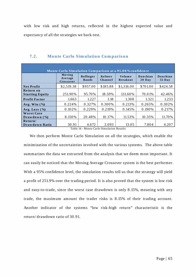
7.2. Monte Carlo Simulation Comparison
Monte Carlo Simulation Comparison at a 95.00% confidence
Moving Average
Crossover
Bollinger Bands
Keltner Channel
Volume Breakout
Donchian 20 Day
Donchian 55 Day
Net Profit $2,519.38 $957.00 $185.88 $1,316.00 $701.00 $424.58 Return on Starting Equity 251.90% 95.70% 18.59% 131.60% 70.01% 42.46%
Profit Factor 1.663 1.227 1.18 1.308 1.321 1.233
Avg. Win (%) 0.224% 0.327% 0.300% 0.213% 0.265% 0.302%
Avg. Loss (%) 0.102% 0.229% 0.219% 0.145% 0.190% 0.217% Worst Case Drawdown (%) 8.150% 20.48% 10.17% 11.53% 10.35% 11.70% Return/ Drawdown Ratio 30.91 4.672 2.093 13.05 7.804 4.207
Table 14 - Monte Carlo Simulation Results
We then perform Monte Carlo Simulation on all the strategies, which enable the
minimization of the uncertainties involved with the various systems. The above table
summarizes the data we extracted from the analysis that we deem most important. It
can easily be noticed that the Moving Average Crossover system is the best performer.
With a 95% confidence level, the simulation results tell us that the strategy will yield
a profit of 251.9% over the trading period. It is also proved that the system is low risk
and easy-to-trade, since the worst case drawdown is only 8.15%, meaning with any
trade, the maximum amount the trader risks is 8.15% of their trading account.
Another indicator of the systems “low risk-high return” characteristic is the
return/drawdown ratio of 30.91.
Page | 65

8. Conclusion
Throughout this MQP we presented six trading strategies with alternating set-ups
and all other aspects ceteris paribus. We back-tested these strategies for the 559 CAN
SLIM Stocks of 2007 and analyzed their performances using two enhanced
comparison techniques - system quality analysis and Monte Carlo simulation.
We combined the two schools of thought in trading. Technical analysis assumes
that market prices at any given point in time reflect all known factors affecting
supply and demand for a particular market. On the other hand, fundamental analysis
is based on the study of factors external to the stock markets which affect the stock
price direction (Covel).
After analyzing and interpreting the data, two strategies stood out – Volume
Breakout and Moving Average Crossover. However, due to the large number of
trades executed by the Volume Breakout strategy, we believe that the Moving
Average Crossover strategy blends the best with the long term investment strategy of
William O’Neal’s CAN SLIM methodology. The Moving Average Crossover system’s
trend-following characteristics aim to take advantage of the long-term price moves of
the CAN SLIM stocks, presenting traders with the opportunity to achieve high
profits.
Page | 66

9. Further Work
Although our study is a comprehensive one, in the scope of our three-term long
project, we were not able to cover all aspects of the matter. In this section we list the
areas which need further research in order to build a fully functioning complete
trading strategy. We suggest further work in the following areas:
• Position sizing and cash management is one of the most important aspects of
a complete trading strategy that we were not able to utilize. It provides traders
with a set of rules on how to diversify their portfolios and how much of their
portfolio they should invest on any given position in the market.
• Commission and slippage costs should be taken into account in order to
retrieve accurate, expected profit values. Although commission costs are very
low these days due to the highly competitive direct access brokerages, we
believe they should be further investigated. Slippage - the difference between
estimated transaction costs and the amount actually paid – is another cost
that could affect the strategy’s overall performance.
• In the scope of our MQP, we only test the affect of the set-up on a complete
trading strategy, leaving all other parts constant. We suggest that various
combinations of the all aspects of a complete trading strategy be tested.
Page | 67

10. References
(n.d.). Retrieved November 24, 2007, from Moneychimp:
http://www.moneychimp.com/features/market_cagr.htm
Average True Range. (n.d.). Retrieved April 23, 2008, from StockCharts:
http://stockcharts.com/school/doku.php?id=chart_school:technical_indicators:aver
age_true_range_atr
Bryant, M. (n.d.). Monte Carlo Analysis. Trading Article Library .
Covel, M. (n.d.). Technical Analysis v. Fundamental Analysis: Difference? Retrieved
April 22, 2008, from TurtleTrader: http://www.turtletrader.com/technical-
fundamental.html
Investopedia. (n.d.). Retrieved April 22, 2008, from Monte Carlo Simulation:
http://www.investopedia.com/terms/m/montecarlosimulation.asp
Lee, R. (n.d.). Capture Profits Using Bands And Channels. Retrieved April 23, 2008,
from Investopedia:
http://www.investopedia.com/articles/forex/06/BandsChannels.asp
O'Neil, W. J. (2002). How to Make Money in Stocks: a winning system in good
times or bad. McGraw-Hill.
Technical Analysis. (n.d.). Retrieved November 28, 2007, from StockCharts.com:
http://stockcharts.com/school/doku.php?id=chart_school:overview:technical_analy
sis
Tharp, V. K. (2006). Expectancy Report. The Van Tharp Institute .
Page | 68

Value Investing. (n.d.). Retrieved April 24, 2008, from Wikipedia:
http://en.wikipedia.org/wiki/Value_Investing
What Are Charts? (n.d.). Retrieved November 28, 2007, from StockCharts.com:
http://stockcharts.com/school/doku.php?id=chart_school:chart_analysis:what_are
_charts
Wright, C. (1998). Trading as a Business. Omega Research, Inc.
Page | 69

11. Appendixes
11.1. Moving Average Crossover Strategy EasyLanguage Code
inputs: Price( Close), FastLength( 9), SlowLength( 18), Displace( 0), ATRLength( 10), NumATRs( 3), InitialStopATRs (5), InitialStopATRLength (2) ; variables: FastAvg( 0 ), SlowAvg( 0 ), FileName("C:\MAC.csv "), tradeStr1(""), profit$(0), longOrShort(""), tt(0), ATRCalc( 0 ), MP( 0 ), PosHigh( 0 ), MMS(0); FastAvg = xAverage( Price, FastLength ) ; SlowAvg = xAverage( Price, SlowLength ) ; ATRCalc = AvgTrueRange( ATRLength ) * NumATRs; MP = MarketPosition ; {Buy and Sell decisions based on the Moving Average Crossover} if CurrentBar > 1 and FastAvg crosses over SlowAvg then Buy ( "BuyMAC" ) next bar at High +1 stop ; If Currentbar > 1 and FastAvg crosses below SlowAvg Then Sell( "SellMAC" ) next bar at Low -1 stop; {Initial MMS} if MarketPosition <> 1 then begin Sell ( "InitialStop" ) next bar at Close - AvgTrueRange( InitialStopATRLength ) * InitialStopATRs stop; MMS = Close - AvgTrueRange( InitialStopATRLength ) * InitialStopATRs; end; {Calculation of a trailing ATR stop} if MP = 1 then begin if MP[1] <> 1 or High > PosHigh then PosHigh = High ; Sell ( "Exit" ) next bar at PosHigh - ATRCalc stop ; end else Sell ( "Exit-eb" ) next bar at High - ATRCalc stop ; {Decision to close the position at the end of the period} If Date >= 1071228 Then Begin Sell ("ClosePosition") next bar at market; end; {Output of the strategy} tt = TotalTrades;
Page | 70

if tt <> tt[1] then begin // a trade just completed if MarketPosition(1) > 0 then longOrShort = " 1" else longOrShort = " -1"; profit$ = MarketPosition(1)*(ExitPrice(1) - EntryPrice(1)) * BigPointValue; tradeStr1 = symbol + "," + ELDateToString(EntryDate(1)) + "," + NumToStr(EntryPrice(1),2) + "," + ELDateToString(ExitDate(1)) + "," + NumToStr(ExitPrice(1),2) + "," + NumToStr(MMS,2) + "," + longOrShort + "," + NumToStr(profit$, 2) + "," + newline; FileAppend(FileName, tradestr1); end;
11.2. Donchian Channel Strategy EasyLanguage Code
inputs: Length( 20 ), ATRLength( 10), NumATRs( 3), InitialStopATRs (5), InitialStopATRLength (2) ; variables: FileName("C:\Stock Analysis_Donchian55.csv"), tradeStr1(""), profit$(0), longOrShort(""), tt(0), MP( 0 ), PosHigh( 0 ), MMS(0), ATRCalc(0); ATRCalc = AvgTrueRange( ATRLength ) * NumATRs; MP = MarketPosition ; Buy ( "BuyDonchian55" ) next bar at HighestFC( High, Length ) + 1 point stop ; {Initial MMS} if MarketPosition <> 1 then begin Sell ( "InitialStop" ) next bar at Close - AvgTrueRange( InitialStopATRLength ) * InitialStopATRs stop; MMS = Close - AvgTrueRange( InitialStopATRLength ) * InitialStopATRs; end; {Calculation of a trailing ATR stop} if MP = 1 then begin if MP[1] <> 1 or High > PosHigh then PosHigh = High ; Sell ( "Exit" ) next bar at PosHigh - ATRCalc stop ; end else Sell ( "Stop" ) next bar at High - ATRCalc stop ; {Decision to close the position at the end of the period} If Date >= 1071228 Then Begin Sell ("ClosePosition") next bar at market; end; {Output of the strategy} tt = TotalTrades; if tt <> tt[1] then begin // a trade just completed if MarketPosition(1) > 0 then longOrShort = " 1" else longOrShort = " -1"; profit$ = MarketPosition(1)*(ExitPrice(1) - EntryPrice(1)) * BigPointValue; tradeStr1 = symbol + "," + ELDateToString(EntryDate(1)) + "," + NumToStr(EntryPrice(1),2) + "," + ELDateToString(ExitDate(1)) + "," + NumToStr(ExitPrice(1),2) + "," + NumToStr(MMS,2) + "," + longOrShort + "," + NumToStr(profit$, 2) + "," + newline; FileAppend(FileName, tradestr1);
Page | 71

end;
11.3. Keltner Channel Strategy EasyLanguage Code
inputs: Price( Close), Length( 20), NumATRs( 1.5), ATRLength( 10), NumATRs( 3) ; variables: Avg( 0 ), Shift( 0 ), UpperBand( 0 ), SetupBuy( false ), CrossingHigh( 0 ), LowerBand( 0 ), CrossingLow( 0 ), SetupSell( false ), FileName("C:\Keltner.csv"), tradeStr1(""), profit$(0), longOrShort(""), tt(0), ATRCalc( 0 ), MP( 0 ), PosHigh( 0 ), SellPrice (0); Avg = AverageFC( Price, Length ) ; Shift = NumATRs * AvgTrueRange( Length ) ; UpperBand = Avg + Shift ; LowerBand = Avg - Shift ; if CurrentBar > 1 and Price crosses over UpperBand then { CB > 1 check used to avoid spurious cross confirmation at CB = 1 } begin SetUpBuy = true ; CrossingHigh = High ; end else if SetupBuy and ( Price < Avg or High >= CrossingHigh + 1 point ) then SetupBuy = false ; if SetupBuy then Buy ( "KeltnerBuy" ) next bar CrossingHigh + 1 point stop ; if CurrentBar > 1 and Price crosses under LowerBand then { CB > 1 check used to avoid spurious cross confirmation at CB = 1 } begin SetUpSell = true ; CrossingLow = Low ; end else if SetupSell and ( Price > Avg or Low <= CrossingLow - 1 point ) then SetupSell = false ; if SetupSell then Sell ( "KeltnerSell" ) next bar at CrossingLow - 1 point stop ; If Date >= 1071228 Then Begin Sell ("ClosePosition") next bar at market; end; {Calculation of a trailing ATR stop} if MP = 1 then begin if MP[1] <> 1 or High > PosHigh then PosHigh = High ; SellPrice = PosHigh - ATRCalc; Sell ( "Exit" ) next bar at SellPrice stop ; end
Page | 72

else Sell ( "Exit-eb" ) next bar at High - ATRCalc stop ; tt = TotalTrades; if tt <> tt[1] then begin // a trade just completed if MarketPosition(1) > 0 then longOrShort = " 1" else longOrShort = " -1"; profit$ = MarketPosition(1)*(ExitPrice(1) - EntryPrice(1)) * BigPointValue; tradeStr1 = symbol + "," + ELDateToString(EntryDate(1)) + "," + NumToStr(EntryPrice(1),2) + "," + ELDateToString(ExitDate(1)) + "," + NumToStr(ExitPrice(1),2) + "," + NumToStr(SellPrice,2) + "," + longOrShort + "," + NumToStr(profit$, 2) + "," + NumToStr(ATRCalc,2) + "," + newline; FileAppend(FileName, tradestr1); end;
11.4. Bollinger Bands Strategy EasyLanguage Code
inputs: BollingerPrice( Close ), TestPriceLBand( Close ), { cross of this price over LowerBand triggers placement of stop order at LowerBand } Length( 20 ), NumDevsDn( 2 ), ATRLength( 10), NumATRs( 3), InitialStopATRs (5), InitialStopATRLength (2); variables: LowerBand( 0 ) , FileName("C:\BBands.csv"), tradeStr1(""), profit$(0), longOrShort(""), tt(0), ATRCalc( 0 ), MP( 0 ), PosHigh( 0 ), SellPrice (0),MMS(0); ATRCalc = AvgTrueRange( ATRLength ) * NumATRs; MP = MarketPosition ; LowerBand = BollingerBand( BollingerPrice, Length, -NumDevsDn ) ; if CurrentBar > 1 and TestPriceLBand crosses over LowerBand then { CB > 1 check used to avoid spurious cross confirmation at CB = 1 } Buy ( "BuyBBand" ) next bar at LowerBand +1 stop ; {Initial MMS} if MarketPosition <> 1 then begin Sell ( "InitialStop" ) next bar at Close - AvgTrueRange( InitialStopATRLength ) * InitialStopATRs stop; MMS = Close - AvgTrueRange( InitialStopATRLength ) * InitialStopATRs; end; {Calculation of a trailing ATR stop} if MP = 1 then begin if MP[1] <> 1 or High > PosHigh then PosHigh = High ;
Page | 73

SellPrice = PosHigh - ATRCalc; Sell ( "Exit" ) next bar at SellPrice stop ; end else Sell ( "Stop" ) next bar at High - ATRCalc stop ; {Output of the strategy} tt = TotalTrades; if tt <> tt[1] then begin // a trade just completed if MarketPosition(1) > 0 then longOrShort = " 1" else longOrShort = " -1"; profit$ = MarketPosition(1)*(ExitPrice(1) - EntryPrice(1)) * BigPointValue; tradeStr1 = symbol + "," + ELDateToString(EntryDate(1)) + "," + NumToStr(EntryPrice(1),2) + "," + ELDateToString(ExitDate(1)) + "," + NumToStr(ExitPrice(1),2) + "," + NumToStr(MMS,2) + "," + longOrShort + "," + NumToStr(profit$, 2) + "," + newline; FileAppend(FileName, tradestr1); end;
11.5. Volume Breakout Strategy EasyLanguage Code
inputs: ATRLength( 10), NumATRs( 3), InitialStopATRs (10), InitialStopATRLength (3) ; variables: FileName("C:\Volume.csv"), tradeStr1(""), profit$(0), longOrShort(""), tt(0), ATRCalc( 0 ), MP( 0 ), PosHigh( 0 ), MMS(0); ATRCalc = AvgTrueRange( ATRLength ) * NumATRs; MP = MarketPosition ; inputs: HoldingPeriod(5), AvgLength( 10 ), BrkOutPct( 50 ) ; variables: BrkOutFactor( 1 + BrkOutPct * .01 ) ; if Volume >= Average( Volume, AvgLength)*BrkOutFactor then Buy ("BuyVolBrkout") next bar at +1 stop; {Initial MMS} if MarketPosition <> 1 then begin Sell ( "InitialStop" ) next bar at Close - AvgTrueRange( InitialStopATRLength ) * InitialStopATRs stop; MMS = Close - AvgTrueRange( InitialStopATRLength ) * InitialStopATRs; end; {Calculation of a trailing ATR stop} if MP = 1 then begin if MP[1] <> 1 or High > PosHigh then PosHigh = High ; Sell ( "Exit" ) next bar at PosHigh - ATRCalc stop ; end else Sell ( "Stop" ) next bar at High - ATRCalc stop ;
Page | 74
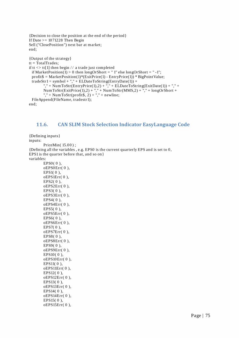
{Decision to close the position at the end of the period} If Date >= 1071228 Then Begin Sell ("ClosePosition") next bar at market; end; {Output of the strategy} tt = TotalTrades; if tt <> tt[1] then begin // a trade just completed if MarketPosition(1) > 0 then longOrShort = " 1" else longOrShort = " -1"; profit$ = MarketPosition(1)*(ExitPrice(1) - EntryPrice(1)) * BigPointValue; tradeStr1 = symbol + "," + ELDateToString(EntryDate(1)) + "," + NumToStr(EntryPrice(1),2) + "," + ELDateToString(ExitDate(1)) + "," + NumToStr(ExitPrice(1),2) + "," + NumToStr(MMS,2) + "," + longOrShort + "," + NumToStr(profit$, 2) + "," + newline; FileAppend(FileName, tradestr1); end;
11.6. CAN SLIM Stock Selection Indicator EasyLanguage Code
{Defining inputs} inputs: PriceMin( 15.00 ) ; {Defining all the variables , e.g. EPS0 is the current quarterly EPS and is set to 0, EPS1 is the quarter before that, and so on} variables: EPS0( 0 ), oEPS0Err( 0 ), EPS1( 0 ), oEPS1Err( 0 ), EPS2( 0 ), oEPS2Err( 0 ), EPS3( 0 ), oEPS3Err( 0 ), EPS4( 0 ), oEPS4Err( 0 ), EPS5( 0 ), oEPS5Err( 0 ), EPS6( 0 ), oEPS6Err( 0 ), EPS7( 0 ), oEPS7Err( 0 ), EPS8( 0 ), oEPS8Err( 0 ), EPS9( 0 ), oEPS9Err( 0 ), EPS10( 0 ), oEPS10Err( 0 ), EPS11( 0 ), oEPS11Err( 0 ), EPS12( 0 ), oEPS12Err( 0 ), EPS13( 0 ), oEPS13Err( 0 ), EPS14( 0 ), oEPS14Err( 0 ), EPS15( 0 ), oEPS15Err( 0 ),
Page | 75

NI0( 0 ), oNI0Err( 0 ), NI1( 0 ), oNI1Err( 0 ), NI2( 0 ), oNI2Err( 0 ), NI3( 0 ), oNI3Err( 0 ), SE0( 0 ), oSE0Err( 0 ), SE1( 0 ), oSE1Err( 0 ), SE2( 0 ), oSE2Err( 0 ), SE3( 0 ), oSE3Err( 0 ), ROE ( 0 ), {The following variables will hold the EPS % Change from quarter to quarter and from year to year} EPSPctChgYr0( 0 ), EPSPctChgYr1( 0 ), EPSPctChgYr2( 0 ), EPSPctChgQrt0( 0 ), EPSPctChgQrt1( 0 ), EPSPctChgQrt2( 0 ), EPSPctChgQrt3( 0 ), counterQrt( 0 ), counterYr( 0 ), AvgClose( 0 ); {The following commands assign fundamental values to the variables, e.g. EPS0 is assigned the EPS value for the current quarter} EPS0 = FundValue( "SDBF", 0, oEPS0Err ) ; EPS1 = FundValue( "SDBF", 1, oEPS1Err ) ; EPS2 = FundValue( "SDBF", 2, oEPS2Err ) ; EPS3 = FundValue( "SDBF", 3, oEPS3Err ) ; EPS4 = FundValue( "SDBF", 4, oEPS4Err ) ; EPS5 = FundValue( "SDBF", 5, oEPS5Err ) ; EPS6 = FundValue( "SDBF", 6, oEPS6Err ) ; EPS7 = FundValue( "SDBF", 7, oEPS7Err ) ; EPS8 = FundValue( "SDBF", 8, oEPS8Err ) ; EPS9 = FundValue( "SDBF", 9, oEPS9Err ) ; EPS10 = FundValue( "SDBF", 10, oEPS10Err ) ; EPS11 = FundValue( "SDBF", 11, oEPS11Err ) ; EPS12 = FundValue( "SDBF", 12, oEPS12Err ) ; EPS13 = FundValue( "SDBF", 13, oEPS13Err ) ; EPS14 = FundValue( "SDBF", 14, oEPS14Err ) ; EPS15 = FundValue( "SDBF", 15, oEPS15Err ) ; NI0 = FundValue( "NINC", 0, oNI0Err ) ; NI1 = FundValue( "NINC", 1, oNI1Err ) ; NI2 = FundValue( "NINC", 2, oNI2Err ) ; NI3 = FundValue( "NINC", 3, oNI3Err ) ; SE0 = FundValue( "QTLE", 0, oSE0Err ) ; SE1 = FundValue( "QTLE", 1, oSE1Err ) ; SE2 = FundValue( "QTLE", 2, oSE2Err ) ; SE3 = FundValue( "QTLE", 3, oSE3Err ) ; {The following calculates the average closing price and checks if is higher than PriceMin} AvgClose = ( close[1] + close[92] + close[183] + close[280] + close[365] )/5; if AvgClose > PriceMin then begin {The following checks if there is any error retrieving the values} if oEPS0Err = fdrOk
Page | 76

and oEPS1Err = fdrOk and oEPS2Err = fdrOk and oEPS3Err = fdrOk and oEPS4Err = fdrOk and oEPS5Err = fdrOk and oEPS6Err = fdrOk and oEPS7Err = fdrOk and oEPS8Err = fdrOk and oEPS9Err = fdrOk and oEPS10Err = fdrOk and oEPS11Err = fdrOk {and oEPS12Err = fdrOk and oEPS13Err = fdrOk and oEPS14Err = fdrOk and oEPS15Err = fdrOk} and oNI0Err = fdrOk and oNI1Err = fdrOk and oNI2Err = fdrOk and oNI3Err = fdrOk and oSE0Err = fdrOk and oSE1Err = fdrOk and oSE2Err = fdrOk and oSE3Err = fdrOk {The following checks if the EPS, NI and SE are greater than 0} {and EPS0 > 0 and EPS1 > 0 and EPS2 > 0 and EPS3 > 0 and EPS4 > 0 and EPS5 > 0 and EPS6 > 0 and EPS7 > 0 and EPS9 > 0 and EPS10 > 0 and EPS11 > 0 and EPS12 > 0 and EPS13 > 0 and EPS14 > 0 and EPS15 > 0 and NI0 > 0 and NI1 > 0 and NI2 > 0 and NI3 > 0 and SE0 > 0 and SE1 > 0 and SE2 > 0 and SE3 > 0} then {The following commands calculate the quarterly and annual EPS Growth, and the ROE} begin ROE = 100* ( ( NI0 + NI1 + NI2 + NI3) / (( SE0 + SE1 + SE2 + SE3)/4) ); EPSPctChgYr0 = 100 * ( (EPS0 + EPS1 + EPS2 + EPS3) - (EPS4 + EPS5 + EPS6 + EPS7)) /(EPS4 + EPS5 + EPS6 + EPS7); if ( EPSPctChgYr0 > 20 ) then counterYr = counterYr + 1; EPSPctChgYr1 = 100 * ( (EPS4 + EPS5 + EPS6 + EPS7) - (EPS8 + EPS9 + EPS10 + EPS11)) /(EPS8 + EPS9 + EPS10 + EPS11); if ( EPSPctChgYr1 > 20 ) then counterYr = counterYr + 1; EPSPctChgYr2 = 100 * ( (EPS8 + EPS9 + EPS10 + EPS11) - (EPS12 + EPS13 + EPS14 + EPS15)) /(EPS12 + EPS13 + EPS14 + EPS15);
Page | 77

if ( EPSPctChgYr2 > 20 ) then counterYr = counterYr + 1; EPSPctChgQrt0 = 100 * ( EPS0 - EPS4 ) / EPS4 ; if ( EPSPctChgQrt0 > 25 ) then counterQrt = counterQrt + 1; EPSPctChgQrt1 = 100 * ( EPS1 - EPS5 ) / EPS5 ; if ( EPSPctChgQrt1 > 25 ) then counterQrt = counterQrt + 1; EPSPctChgQrt2 = 100 * ( EPS2 - EPS6 ) / EPS6 ; if ( EPSPctChgQrt2 > 25 ) then counterQrt = counterQrt + 1; EPSPctChgQrt3 = 100 * ( EPS3 - EPS7 ) / EPS7 ; if ( EPSPctChgQrt3 > 25 ) then counterQrt = counterQrt + 1; {The counters are used to determine whether there are at least 2 quarters in the last year with EPS growth of at least 25% and whether the annual EPS growth for the last 3 years is more than 20%} if counterQrt >=2 and counterYr >=2 and ROE > 17 then begin {The following commands display the values in columns in RadarScreen if EPSPctChgYr0 > 0 then begin Plot1( EPSPctChgYr0, "AEG Now", Green ) ; end else begin Plot1( EPSPctChgYr0, "AEG Now", Red ) ; end; if EPSPctChgYr1 > 0 then begin Plot2( EPSPctChgYr1, "AEG -1", Green ) ; end else begin Plot2( EPSPctChgYr1, "AEG -1", Red ) ; end; if EPSPctChgYr2 > 0 then begin Plot3( EPSPctChgYr2, "AEG -1", Green ) ; end else begin Plot3( EPSPctChgYr2, "AEG -1", Red ) ; end; if EPSPctChgQrt0 > 0 then begin Plot4( EPSPctChgQrt0, "EPS Chg Now", Green ) ; ; end else begin Plot4( EPSPctChgQrt0, "EPS Chg Now", Red ) ; end; if EPSPctChgQrt1 > 0 then begin Plot5( EPSPctChgQrt1, "EPS Chg Now", Green ) ; ; end else begin Plot5( EPSPctChgQrt1, "EPS Chg Now", Red ) ; end;
Page | 78

Page | 79
if EPSPctChgQrt2 > 0 then begin Plot6( EPSPctChgQrt2, "EPS Chg Now", Green ) ; ; end else begin Plot6( EPSPctChgQrt2, "EPS Chg Now", Red ) ; end; if EPSPctChgQrt3 > 0 then begin Plot7( EPSPctChgQrt3, "EPS Chg Now", Green ) ; ; end else begin Plot7( EPSPctChgQrt3, "EPS Chg Now", Red ) ; end; Plot8( ROE, "ROE" ) ; Plot9(AvgClose, "Stock Price", Green); end else {If the stock does not qualify for our critera, the following is displayed} Plot10( "No Match", "Error", Red ) ; end {If there is not enough data, the following is displayed} else Plot10( "Data N/A", "Error", Red ) ; end else Plot10( "No Match", "Error", Red);
11.7. CAN SLIM Stock Selection (Symbols)
A AAON AAPL AAWW ABB ABI ABR ABT ACAP ACAS ACGL ACGY ACH ACL ACN ADI ADM ADSK AEO AEPI AET AFAM AHL AIRM AIT AIZ AJG AKS
ALB AMAT AME AMG AMGN AMN AMPH AMX AMZN ANDE ANR ANST APD APH APOG APOL ARA ARGN ARKR ARO ARP ARTW ASFI ASML ATI ATK ATLS ATNI
ATRI ATRO ATW AVTR AWC AXA AXE AYI AZ AZZ B BA BAP BAX BBNK BBV BBY BCPC BCR BCS BDK BDX BEC BEN BGC BHI BHP BID
BIDU BIG BKC BKE BLKB BLL BLUD BMC BMY BOLT BOOM BRLI BRY BT BUCY BVN BW BXP BYD CACC CADA CAE CAG CALM CAM CB CBE CBG
CBI CE CEO CF CG CHKE CHL CHRW CHTT CL CLB CLHB CLP CM CMC CMTL CNC CNI CNP CNQ CNX COH COKE COL CPA CPL CRDN CRS

CRVL CS CSCO CSL CTBK CTRP CTSH CTV CUZ CVD CVH CX CY D DAL DB DDMX DE DECK DHIL DIOD DISH DKS DLB DLLR DLX DNA DNEX DNR DO DPL DRQ DST DSW DSX DVA DVN DWSN DXPE E EAT EBIX EGN EL ELS ENL EPAX ERIC ERIE ESI ESRX ESV EXC EXM FCSX FCX FDO FDS FLIR FLR FLS
FRGB FRO FRX FSTR FTI FTK FTO FWLT GD GDI GEF GEOY GES GFIG GGP GHL GIGM GIL GILD GLBL GLF GLNG GLW GM GMT GOOG GPOR GR GRMN GRP GS GT GWW GYMB HAL HANS HAR HAS HAYN HBC HCC HES HIBB HITT HLF HLX HME HNP HNZ HOC HON HOT HP HPQ HPY HRBN HRS HSC HSII HUBG HUM
HURC HURN HXM ICE IDCC IFF IIVI IMKTA INFA INFY ING ININ INTC IP IRE ISRG ITMN ITT ITY JBHT JBX JCG JCOM JEC JLL JOSB JWN KALU KCI KEX KMB KR KSS KTC KTII LABL LCAV LDSH LECO LEH LH LHCG LIFC LLY LMT LOGI LPHI LRCX LTD LTRE LUFK LUX MA MAN MBT MCHP MCRI MDR MDU MEOH MET
MGM MHP MICC MIDD MITSY MKC MLAB MLHR MLI MLM MMM MNT MORN MOS MRH MSFT MSM MT MTD MTL MTW MUR MVL MW MXGL NATH NATI NATL NCIT NDAQ NE NEU NFG NGG NHI NHP NIHD NILE NJR NKE NMX NNDS NOK NOV NRGP NSR NTG NTRI NTY NU NVDA NVEC NVO NVT NVTL NWL OC OII OMCL OMG OPY
ORCL ORH OSK OXPS OXY OYOG PBR PCLN PCP PCR PCU PCZ PDE PEG PENN PEP PETM PHG PHLY PKG PKOH PKX PLD PMTC POT PPG PTEN PTNR PTR PUK PVH PX PXP PZZA QCOM QDEL QSII RBA RDC REP RIG RIMM RIO RLI ROK ROLL ROST RPT RS RSH RTI RTN RTP RUK RY RYAAY RYN SAN SAY SCHW SEE
Page | 80

Page | 81
SEPR SGP SHOO SI SID SIGM SII SILC SIMO SIVB SJR SKM SLAB SLB SLG SM SNDA SNHY SNP SOHU SPN SPTN SRCL SSL STAN STJ STLD STO STRA STX SUN SUNH SURW SWSI SYK SYNA SYNL SYNT TBSI TCK TCO TD TDW TDY TE TECH TEF TEX TIE TIF TISI TKC TKG TLK TMX TNB TNP TOC TOT TPX TRMD
TRN TROW TRV TS TSO TSS TTC TUP TV TWGP TWIN TXT UA UBS UGI UL UN UNH URBN USNA UTHR VCP VDSI VE VIP VIVO VLCM VLO VMC VMI VSEA VSEC VSNT WAB WAT WBD WBK WCC WCG WDC WDR WFR WGOV WHG WHQ WHR WINN WPPGY WST WXS XRAY YZC ZU
