2

Table of Contents

List of Acronyms and Abbreviations .................................................................................................................... 3

Part 1. Recent Economic Developments ............................................................................................................. 4

1.1 Growth: after almost two years of recession, Russia entered a path to recovery ................................. 12

1.2 Balance of payments: stable despite substantial external volatility. ...................................................... 17

1.3 Labor Market and Poverty Trends: unemployment is stable and wages are recovering, but economy-

wide unit labor costs are increasing faster than the OECD average and they vary across sectors. ............. 20

1.4 Monetary Policy: gradual monetary easing amidst an uncertain and volatile external environment. .. 23

1.5 The Financial Sector: the banking system has largely stabilized, but has not yet fully recovered and

credit growth remains stalled. ...................................................................................................................... 26

1.6 Government Budget: important actions have been taken in preparation for a new fiscal rule............. 28

Part 2. The outlook for three years: growth prospects are modest ................................................................. 33

Part 3. Russian regions and their responses during the crisis years ................................................................. 43

Functions ....................................................................................................................................................... 45

Financing ....................................................................................................................................................... 46

Fiscal Performance ........................................................................................................................................ 48

Prognosis ....................................................................................................................................................... 51

SHORT-TERM MEASURES .......................................................................................................................... 52

LONG-TERM MEASURES ............................................................................................................................ 53

References ......................................................................................................................................................... 54

3

List of Acronyms and Abbreviations

Bbl Oil barrel

CBR Central Bank of Russia

CDS Credit-Default Swap

CES Constant Elasticity of Substitution

CIT Corporate Income Tax

CPI Consumer Price Index

DIA Deposit Insurance Agency

EMDE Emerging Market and Developing Economies

EU European Union

GDP Gross Domestic Product

HIF Health Insurance Fund

IEA International Energy Agency

IP Industrial Production

LFP Labor Force Participation

M2 Money Supply

NPL Nonperforming Loan

OECD Organization for Economic Cooperation and Development

OPEC Organization of the Petroleum Exporting Countries

PIT Personal Income Tax

PPP Purchasing Power Parity

REER Real Effective Exchange Rate

RER Real Exchange Rate

ULC Unit Labor Cost

WDI World Development Indicators

y/y Year-on-year

SAAR Seasonally Adjusted Annualized Rate

4

Russia: From Recession to Recovery

Executive Summary

Global growth started to strengthen at the end of 2016. After a slowdown of growth to 2.3 percent in 2016 driven by weak investment and trade, global growth started to improve at the end of 2016 (Figure 1.a). Investment and exports are gaining momentum, albeit muted by still feeble private consumption. An upturn in the US and steady growth in the Euro Area and Japan are supporting the upward trend. In China, strong public and state-owned companies’ infrastructure spending slowed the rebalancing trend from investment to consumption, although the structural shifts from manufacturing to services and from external demand to domestic demand continued.

Global trade also recovered, and global financing

conditions for emerging economies remained benign in

early 2017. From its low point in 2013, trade growth

recovered in the second half of 2016, supported by

improved industrial activity (Figure 2.a). Global

financing conditions were favorable in early 2017. While

the U.S. long-term yield increased by 50 basis points and

currencies in many emerging markets depreciated after

the U.S. elections of November 2016, the increase was

not accompanied by a sustained re-pricing of risk and of

emerging-market assets. Capital inflows to emerging

and developing economies were robust in the first half

of 2017.

Amidst weakening external headwinds, rising oil prices, and growing macro-stability, the Russian economy

showed encouraging signs of overcoming the recession it entered in 2014. In 2016, Russia’s GDP contracted

by 0.2 percent, y/y, compared to a 2.8 percent contraction in 2015, with the economy bottoming out in the

first quarter of 2016 (Figure 3.a). The incipient positive momentum appears to have spilled into 2017. In the

first quarter of 2017, GDP grew by 0.5 percent, y/y. In the first four months of 2017, industrial production

expanded by 0.7 percent y/y. In the first quarter of 2017, agriculture also grew by 0.7 percent, y/y, and PMI

indexes for both manufacturing and services pointed to expansion (Figure 4.a). Growing macro-stability driven

by the government’s policy response package of a flexible exchange rate policy, expenditure cuts, and bank

recapitalization – along with tapping the Reserve Fund – has helped facilitate this adjustment. Box 1 in the

report highlights the varying implications of the oil price shock on oil exporters, and how Russia has adapted

well compared to others.

Figure 1.a: Global Growth is strengthening

Source: World Bank. AE = Advanced Economies. EMDE = Emerging Markets and Developing Economies. Series are seasonally adjusted.

Figure 2.a: Global Industrial Production is growing

Source: Global Monthly, World Bank.

0

2

4

6

2011 2012 2013 2014 2015 2016

AE Global EMDEPercent, yoy

5

Figure 3.a: The Russian economy bottomed out in the first quarter of 2016 (GDP growth, percent, y/y and q/q) sa

Figure 4.a: Positive momentum appears to have rolled over to 2017 (IP, agriculture and cargo turnover growth, percent, y/y)

Source: Rosstat, Ministry of Economic Development. Source: Rosstat.

Headline Russian economic and financial trends

and indicators are improving. A moderately tight

monetary stance helped reduce the average

inflation rate from 15.6 percent in 2015 to 7.1

percent in 2016. Headline inflation almost reached

the end-year target of 4 percent as early as April

2017, falling to 4.1 percent, y/y. (Figure 5.a).

Recognizing that several one-off factors supported

the reduction in headline inflation, the Bank of

Russia pursued a cautious approach to monetary

easing as inflation expectations, although following

a downward trend, remained elevated.

Employment and labor force participation rates

were still near maximum historical levels, while

unemployment was close to the minimum (Figure 6.a). The banking sector showed signs of increased stability

and a return to pre-crisis profitability levels. Key credit risk and performance indicators remained largely

unchanged (Figure 7.a), signaling that the worsening trend may be over. Capital adequacy remained stable at

around 13 percent.

-4.0

-3.0

-2.0

-1.0

0.0

1.0

2.0

Q12014

Q22014

Q32014

Q42014

Q12015

Q22015

Q32015

Q42015

Q12016

Q22016

Q32016

Q42016

SA q/q y-o-y

0

10

20

30

40

50

60

70

92

94

96

98

100

102

104

106

108

110

Industrial Production Cargo

Agriculture PMI services (RHS)

PMI manufacturing (RHS)

Figure 5.a: Inflation has slowed down (CPI index and its

components (percent, y/y)

Source: CBR and Haver Analytics.

Figure 6.a: Employment and Labor Force Participation

rates are high (percent)

Figure 7.a: Key credit risk and performance trends are holding steady

Source: Rosstat, Haver Analytics and World Bank staff estimates.

Source: CBR.

62

63

64

65

66

67

68

69

70

71

2011 2012 2013 2014 2015 2016

LFP rate Employment rateLFP rate, MA Empl. rate, MA

6

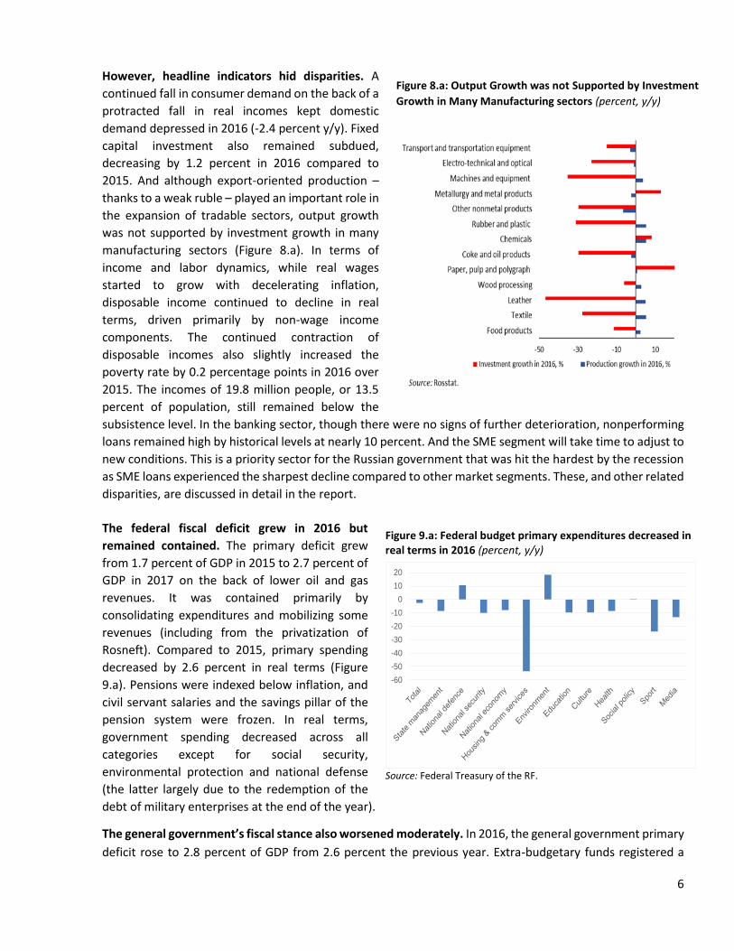
However, headline indicators hid disparities. A

continued fall in consumer demand on the back of a

protracted fall in real incomes kept domestic

demand depressed in 2016 (-2.4 percent y/y). Fixed

capital investment also remained subdued,

decreasing by 1.2 percent in 2016 compared to

2015. And although export-oriented production –

thanks to a weak ruble – played an important role in

the expansion of tradable sectors, output growth

was not supported by investment growth in many

manufacturing sectors (Figure 8.a). In terms of

income and labor dynamics, while real wages

started to grow with decelerating inflation,

disposable income continued to decline in real

terms, driven primarily by non-wage income

components. The continued contraction of

disposable incomes also slightly increased the

poverty rate by 0.2 percentage points in 2016 over

2015. The incomes of 19.8 million people, or 13.5

percent of population, still remained below the

subsistence level. In the banking sector, though there were no signs of further deterioration, nonperforming

loans remained high by historical levels at nearly 10 percent. And the SME segment will take time to adjust to

new conditions. This is a priority sector for the Russian government that was hit the hardest by the recession

as SME loans experienced the sharpest decline compared to other market segments. These, and other related

disparities, are discussed in detail in the report.

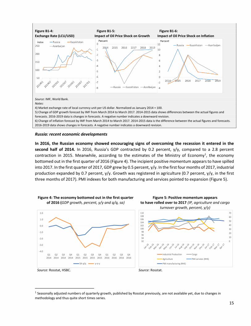
The federal fiscal deficit grew in 2016 but

remained contained. The primary deficit grew

from 1.7 percent of GDP in 2015 to 2.7 percent of

GDP in 2017 on the back of lower oil and gas

revenues. It was contained primarily by

consolidating expenditures and mobilizing some

revenues (including from the privatization of

Rosneft). Compared to 2015, primary spending

decreased by 2.6 percent in real terms (Figure

9.a). Pensions were indexed below inflation, and

civil servant salaries and the savings pillar of the

pension system were frozen. In real terms,

government spending decreased across all

categories except for social security,

environmental protection and national defense

(the latter largely due to the redemption of the

debt of military enterprises at the end of the year).

The general government’s fiscal stance also worsened moderately. In 2016, the general government primary

deficit rose to 2.8 percent of GDP from 2.6 percent the previous year. Extra-budgetary funds registered a

Figure 8.a: Output Growth was not Supported by Investment

Growth in Many Manufacturing sectors (percent, y/y)

Figure 9.a: Federal budget primary expenditures decreased in real terms in 2016 (percent, y/y)

Source: Federal Treasury of the RF.

-60

-50

-40

-30

-20

-10

0

10

20

7

marginal deficit of 0.2 percent of GDP, and imbalances in the pension system increased. Federal government

transfers that covered the Pension Fund deficit grew to 2.4 percent of GDP from 2.1 percent of GDP in 2015,

reflecting a substantial dependence of the Pension Fund on the federal budget.

There are significant variations in the quality of the

regional budgets and concerns related to the growing

role of federal government loans. The consolidated

regional budget registered a primary surplus of 0.2

percent of GDP in 2016. And as Part 3 of the report

discusses in detail, Russian regions have weathered the

slowdown in the economy fairly well in the recent past

– showcasing low deficits and broadly moderate debt

levels. However, the structure of the local debt presents

challenges, as it is mostly made up of short maturities

and subject to rollover risks. The significant part of

subnational debt (39 percent) shown in Figure 10.a

takes the form of short-term loans from commercial

banks. In addition, some local governments are highly indebted.

Adjustment in Russian regions has happened through massive expenditure cuts as opposed to revenue

mobilization, with social sectors and capital spending hit the hardest. Better debt management (reducing

rollover risks; mobilizing more revenues and cutting expenditures where it makes sense) will be key to

unlocking the growth potential at subnational levels, as will improving the public-sector efficiency of

subnational governments.

In early 2017, the federal government balance strengthened on the back of increasingly robust oil revenues.

Compared to January – March 2016, oil and gas revenues in the federal budget rose by 2.2 percent of GDP to

7.6 percent of GDP on the back of higher oil prices. Federal budget primary expenditures increased by 0.2

percent of GDP to 18.6 percent of GDP. The federal government balance consequently registered a primary

deficit of 0.5 percent of GDP in January-March 2017

compared to -2.4 percent of GDP deficit in the same

period last year. However, the federal non-oil

primary deficit worsened marginally to 8.0 percent

of GDP in January-March 2017 on the back of higher

expenditures, compared to 7.9 percent of GDP in

the same period last year.

With an eye to the proposed introduction of the

new fiscal rule, the government passed a three-

year federal budget law and introduced currency

interventions in the domestic market. The three-

year budget law covering the 2017-2019 period

provides for substantial fiscal consolidation, mainly

through expenditure cuts and limited revenue

Figure 10.a: Short-term loans account for over one-third of the subnational debt

Source: Federal Treasury of the RF.

Figure 11.a: Federal budget deficit expected to

decrease over time (percent of GDP)

Source: Ministry of Finance of the RF.

-3,6

-3,2

-2,2

-1,2

-4

-3,5

-3

-2,5

-2

-1,5

-1

-0,5

0Actual Budgetlaw

2016 2017 2018 2019

8

mobilization efforts. The budget law is based on an oil price of US$ 40/bbl for the 2017-2019 period (Figure

11.a).

Expenditure consolidation – more than revenue mobilization – is the central plank of the three-year federal

budget law. Compared to 2016, federal budget primary expenditures would decrease by about 7 percent in

real terms (deflated by CPI) over three years and by 3.6 percent of GDP, almost evenly distributed, with the

biggest expenditure cuts proposed in national defense, the national economy and in housing and communal

services. In real terms, all federal budget expenditure categories would decrease over three years except for

environmental protection. Social policy expenditures would decrease by 2.5 percent in real terms in 2019

compared to 2016, which would require increased targeting of these expenditures. The fiscal consolidation

will also be supported by some revenue mobilization efforts: the government projects to raise 1.1 percent of

GDP in 2017-2019 predominantly from the transfer of dividends of state-controlled companies and by

increasing tax revenue from the energy sector. As Box 3 in the report and Figure 12.a shows below, Russia’s

expenditures as share of GDP are low compared to other countries, suggesting more emphasis could perhaps

be paid to mobilizing revenues in addition to expenditure cuts.

Figure 12.a: Russia’s expenditures as % of GDP are low compared to other countries’ General Government spending as percentage of GDP and by function:

Russia vs. EU-28 and OECD average for 2015

Source: OECD, Federal Treasury of the RF, Eurostat.

0 5 10 15 20 25 30 35 40 45 50

TOTAL

General public services

Defense

Public order and safety

Economic affairs

Environmental protection

Housing and community amenities

Health

Recreation, culture and religion

Education

Social protection

2015

OECD average (27 countries) EU-28 Russia

9

Against these dynamics, we expect the economy

to go from recession to recovery. Consistent with

our projections in the previous Russia Economic

Report (November 2016), we expect the Russian

economy to grow 1.3 percent in 2017 and 1.4

percent both in 2018 and 2019 (Figure 13.a). The

positive terms-of-trade effect from rising oil

prices, coupled with more stable macroeconomic

conditions, are expected to drive this recovery.

And as Box 5 in the report elaborates, being

among the top three oil exporters in the world,

the Russian oil sector has demonstrated

resilience, increasing production and exports

despite headwinds, thanks to increased

production by small- and medium-size producers (including Gazpromneft, Novatek, Tatneft, Russneft, and

Bashneft). Moreover, total oil production is expected to increase to 11.38 mb/d in 2017 and peak at 11.54

mb/d in 2018, as new projects will more than offset brownfield declines.

Consumption is expected to drive growth in 2017-2019 with investment playing a supporting role (Table

1.a). We expect headline inflation to continue moderating, falling slightly below 4 percent at the end of 2017

and stabilizing around 4 percent in 2018-2019. Lower inflation will support real wages that will be the main

source of real income growth. These and improving consumers’ sentiments and better credit conditions are

all expected to lead to a growth in private consumption of 1.8 percent in 2017 and 2.5 percent in 2018 and

2019. Investment demand is also expected to pick up in the forecasting period as businesses renew their

stocks in 2017 and fixed capital investment grows due to macro stabilization and improved investors’

sentiment. The 2018 soccer World Cup could further support public investment. The contribution of net

exports to growth is expected to be negative in 2017 as import growth is expected to outstrip export growth

in 2017 because of an improvement in domestic demand fueled by inventory restocking and deferred demand

for investment imports. Table 1 shows the projected overall growth, growth in its expenditure components,

as well as the components’ contribution to projected growth.

Table 1.a: Projected growth is between 1.3 to 1.4 percent in 2017 - 2019

Projected Growth, y/y, percent Contribution to Growth, pp

2017 2018 2019 2017 2018 2019

GDP 1.3 1.4 1.4 1.3 1.4 1.4

Consumption 1.1 1.6 1.6 0.7 1.0 1.1

Gross capital formation 8.0 1.5 1.1 1.5 0.3 0.2

Gross fixed capital

formation 2.0 2.5 3.5 0.4 0.5 0.7

Export 2.0 2.3 2.5 0.6 0.7 0.8

Import 10.0 4.0 4.0 -1.5 -0.6 -0.7

Source: World Bank staff calculations.

Figure 13.a: The economy is expected to grow in 2017-2019

(real GDP growth, percent)

Source: Rosstat, World Bank staff calculations.

10

Growth projections remain sensitive to oil prices.

A simulated decrease of 15 percent in oil prices

reduces growth to 1 percent in 2017 and 1.2

percent for 2018 and 2019 (Figure 15.a). A

simulated increase of 15 percent in oil prices

increases growth to 1.6 percent for 2017 and 1.8

percent for 2018 and 2019. Despite policy efforts

to reduce sensitivity, oil price volatility would still

affect consumer and producer sentiments. We

expect a slightly higher response of the economy

to the upper oil price variation due to improved

investor sentiments.

The poverty rate is expected to decrease because

of decelerated inflation and recoveries in private incomes and consumption. In the baseline oil price

scenario, the poverty headcount is projected to decline in 2017 to 13 percent from 13.5 percent in 2016, and

to continue declining to 12.3 and 11.6 percent in 2018 and 2019 respectively (Figure 16.a). Incomes will also

be supported by an increase in pensions that were indexed by end-year inflation and are likely to increase in

real terms during 2017. Figure 3 also shows the sensitivity of poverty projections to the minus/plus 15-percent

change in oil prices (scenarios 2 and 3) compared to the baseline.

Figure 16.a: The poverty headcount is likely to decline in 2017 and further (percent)

Source: Rosstat, World Bank staff calculations.

0.406

0.408

0.410

0.412

0.414

0.416

0.418

0.420

0.422

10

11

11

12

12

13

13

14

14

2009 2010 2011 2012 2013 2014 2015 2016 2017 2018 2019Poverty rate, % Scenario 1 (baseline) Scenario 2 (lower-bound)

Figure 15.a: GDP growth scenarios in 2017-2019 (percent)

Source: World Bank staff calculations.

11

The medium-term prognosis of the Russian

economy is favorable. Projected growth rates

are between 1.3 to 1.4 percent in the

forecasting period of 2017-2019. Among

factors driving this recovery, maintaining

macro stability and high oil prices are the

most influential. Moreover, the return to the

medium-term fiscal framework and the

introduction of an updated fiscal rule are

expected to further improve economic

predictability. The projected strengthening of

domestic demand is also expected to support

economic activity in the non-tradable and

tradable parts of the economy (Figure 18.a).

However, Russia’s longer-term growth

prospects remained constrained by its low productivity. Box 7 in the report discusses various methods and

measures of total factor productivity (TFP) growth in Russia, all which yield the same conclusion as

summarized in Figure 19.a: TFP growth in Russia is low and declining. For example, even in a relatively well-

performing sector like agriculture, as Box 6 in the report illustrates, although revenues and profitability have

increased in the subsectors of pork production and dairy farming, untapped opportunities remain to improve

land and capital productivity. With low TFP growth and a shrinking working age population, potential output

growth is modest at best (around 1 to 1.5 percent of GDP), thus limiting GDP recovery growth rates.

Additionally, as shown in Figure 20.a below, over the past nine years, unit labor costs (ULC) in Russia have

been rising. And as discussed in Box 2, even considering the recent ruble depreciation, high ULCs adversely

affect competitiveness of the Russian economy vis-à-vis other countries.

Boosting productivity growth remains key to achieving inclusive, sustainable and fast-paced growth in Russia.

Figure 18.a: Recovery is broad-based, with both tradable and non-tradable sectors to benefit: Projected growth by sector

Source: World Bank staff calculations.

Figure 19.a: TFP growth (by various measures) is Russia is low and declining

Figure 20.a: Unit Labor Costs (ULC) increased significantly in Russia in recent years

-2

0

2

4

6

8

10

12

1998 2000 2002 2004 2006 2008 2010 2012 2014 2016

CES

Structural change

Education and resources

% change

Source: OECD, Rosstat, Haver Analytics and World Bank staff estimates.

Source: World Bank staff calculations using WDI, Rosstat and

ILO data. Note: CES = Constant Elasticity of Substitution

Source: OECD, Rosstat, Haver Analytics and World Bank staff estimates.

-2

-1

0

1

2

3

4

2016 2017 2018 2019

Agriculture Industrial production Services

12

Part 1. Recent Economic Developments

1.1 Growth: after almost two years of recession, Russia entered a path to recovery

Global growth and trade started to strengthen at the end of 2016. Russia’s economy showed signs of overcoming the recession caused by the shocks of low oil prices and economic sanctions. Tradable sectors benefitted from the relative price adjustment and stabilizing commodity prices in the second half of 2016 and became the main drivers of economic growth, partly through increased exports. There was positive momentum in non-tradable sectors as well, which slowed the pace of contraction compared to 2015. The incipient positive momentum appears to have spilled into early 2017.

13

Global economic trends

Global growth started to strengthen at the end of 2016. After a slowdown to 2.3 percent in 2016 driven by

weak investment and trade, global growth started to improve at the end of 2016 (Figure 1). Investment and

exports gained momentum, although private consumption remained feeble. An upturn in the US and steady

growth in the Euro Area and Japan supported the upward trend. In China, strong public and state-owned

companies’ infrastructure spending slowed the rebalancing trend from investment to consumption, although

the structural shifts from manufacturing to services and from external demand to domestic demand

continued. China’s economy expanded by 6.7 percent, in line with its government’s plans and expectations

(Figure 2).

Figure 1: Global growth is strengthening Figure 2: China: actual and targeted growth in line

Source: World Bank. AE stands for advanced economies. Series are seasonally adjusted.

Source: Global Monthly, World Bank.

Global trade bottomed out and external financing conditions for the emerging economies remained benign.

From its low point in 2013, trade growth recovered in the second half of 2016, supported by improved

industrial activity (Figure 3). Global financial conditions remained positive in early 2017. While the U.S. long-

term yield increased by 50 basis points and currencies in many emerging markets depreciated after the U.S.

elections of November 2016, this increase was not accompanied by a sustained re-pricing of risk and of

emerging-market assets. As a result, capital inflows to emerging and developing economies were robust in

the first half of 2017.

Figure 3: Global industrial production supported recovery in trade growth

Source: Global Monthly, World Bank.

0

2

4

6

2011 2012 2013 2014 2015 2016

AE Global EMDEPercent, yoy

4

6

8

10

12

14

16

20

04

20

05

20

06

20

07

20

08

20

09

20

10

20

11

20

12

20

13

20

14

20

15

20

16

20

17f

Target GDP

Real GDP

Year-on-year, percent

14

Box 1: Varying implications of an oil price shock: Russia had adapted well compared to other oil exporters

Oil prices plunged by 77% from June 2014 to January 2016, severely undermining the activities of energy exporters. However, the macroeconomic implications of the shock varied across countries. This box reports the divergences among oil exporters to provide a cross-country perspective on the situation in Russia.

Exchange-rate flexibility plays a key role in cushioning an export-price shock (IMF 2016). Figure B1-1 shows the impact of the oil price shock on growth, measured by the change in growth forecasts before the oil price shock and after the oil price shock for countries with and without flexible exchange rates, and for Russia. Figures B1-2 and B1-3 shows the impact on inflation and the current account. While the 2014-15 period marked most of the decline in oil prices, countries with an inflexible exchange-rate regime experienced modest decline in growth, due in part to supportive fiscal measures and an absence of high inflation. However, current accounts in inflexible exchange-rate regimes worsened significantly during the same period. Furthermore, by 2017, growth declined sharply in these economies. Five years after the oil shock, growth is expected to continue to drag. In contrast, countries with flexible exchange-rate regimes experienced both an earlier and smaller decline in growth, with growth expected to broadly recover in the five years following the shock. The implications for the current account were minimal.

For Russia, growth adjustment happened earlier than for many oil exporters, reflecting the early impact of economic sanctions and the high inflation associated with the introduction of a floating exchange-rate regime. Exchange-rate pass-through is high when monetary policy credibility is not well established (Carriere-Swallow et al, 2016). Stabilizing exchange rates and inflation contributed to the V-shape recovery in 2016-17, reflecting increasing monetary credibility in Russia.

Figure B1-1: Figure B1-2: Figure B1-3:

Impact of Oil Price Shock on Growth Impact of Oil Price Shock on Inflation Impact of Oil Price Shock on the Current Account

Source: IMF, World Bank.

Notes:

1-3) Samples are energy-exporting emerging economies and frontier markets. Exchange-rate regime classification is as of 2014, and inflexible

exchange rates include peg and no separate legal tender. Countries with flexible exchange rates include Colombia, Ghana, and Indonesia. Countries

with inflexible exchange rates include Bahrein, Bolivia, Ecuador, Gabon, Kuwait, Oman, Qatar, Saudi Arabia, and Venezuela. Azerbaijan, Nigeria,

Malaysia, and Kazakhstan. They are excluded from the sample because they are managed floats. The numbers are the medians of each country

group. 2014-2015 data is the difference between the actual figures and forecasts. 2016-2019 data shows the difference in forecasts. The negative

number indicates downward revision.

1) Change of GDP growth forecast by IMF from March 2014 to March 2017.

2) Change of inflation forecast by IMF from March 2014 to March 2017.

3) Change of current account forecast (percent of GDP) by IMF from March 2014 to March 2017.

In the Europe and Central Asia region, in addition to Russia, Azerbaijan and Kazakhstan moved toward more exchange-rate flexibility (Figure B1-4,5,6). The Russian ruble started to depreciate in late 2014, which led to the acceleration of inflation and a growth slowdown in 2015. Conversely, depreciation of the Kazakh tenge and the Azerbaijani manat started in 2015, and inflation picked up in 2016. While the adjustments to the low oil prices are close to complete in 2017 for Russia, adjustments in Azerbaijan and Kazakhstan are expected to continue in 2017 and beyond. Currency depreciation and economic slowdown have aggravated the banking sector’s balance sheets in Azerbaijan and Kazakhstan, weighing on investment growth.

15

Figure B1-4: Figure B1-5: Figure B1-6:

Exchange Rate (LCU/USD) Impact of Oil Price Shock on Growth Impact of Oil Price Shock on Inflation

Source: IMF, World Bank.

Notes:

4) Market exchange rate of local currency unit per US dollar. Normalized as January 2014 = 100.

5) Change of GDP growth forecast by IMF from March 2014 to March 2017. 2014-2015 data shows differences between the actual figures and

forecasts. 2016-2019 data is changes in forecasts. A negative number indicates a downward revision.

6) Change of inflation forecast by IMF from March 2014 to March 2017. 2014-2015 data is the difference between the actual figures and forecasts.

2016-2019 data shows changes in forecasts. A negative number indicates a downward revision.

Russia: recent economic developments

In 2016, the Russian economy showed encouraging signs of overcoming the recession it entered in the

second half of 2014. In 2016, Russia’s GDP contracted by 0.2 percent, y/y, compared to a 2.8 percent

contraction in 2015. Meanwhile, according to the estimates of the Ministry of Economy1, the economy

bottomed out in the first quarter of 2016 (Figure 4). The incipient positive momentum appears to have spilled

into 2017. In the first quarter of 2017, GDP grew by 0.5 percent, y/y. In the first four months of 2017, industrial

production expanded by 0.7 percent, y/y. Growth was registered in agriculture (0.7 percent, y/y, in the first

three months of 2017). PMI indexes for both manufacturing and services pointed to expansion (Figure 5).

Figure 4: The economy bottomed out in the first quarter of 2016 (GDP growth, percent, y/y and q/q, sa)

Figure 5: Positive momentum appears to have rolled over to 2017 (IP, agriculture and cargo

turnover growth, percent, y/y)

Source: Rosstat, HSBC. Source: Rosstat.

1 Seasonally adjusted numbers of quarterly growth, published by Rosstat previously, are not available yet, due to changes in

methodology and thus quite short times series.

-4.0

-3.0

-2.0

-1.0

0.0

1.0

2.0

Q12014

Q22014

Q32014

Q42014

Q12015

Q22015

Q32015

Q42015

Q12016

Q22016

Q32016

Q42016

SA q/q y-o-y

0

10

20

30

40

50

60

70

92

94

96

98

100

102

104

106

108

110

Industrial Production Cargo

Agriculture PMI services (RHS)

PMI manufacturing (RHS)

16

In 2016, private consumption contracted as

inventory stock decreased, both on a smaller

scale than in 2015. Net exports contributed

positively. Fixed capital investment remained

subdued. A continued fall in consumer demand

on the back of a protracted fall in real incomes

kept domestic demand depressed (-2.4 percent

y/y). However, the pace of contraction slowed

down considerably, compared to 2015, as

consumer confidence improved. The inventory

stock decreased as well, but on a smaller scale

than in in 2015. Increasing exports (+3.1

percent y/y) and contracting imports (-3.8

percent, y/y) became the main engines for GDP

growth (Figure 6).

Export-oriented production played an important role in the expansion of tradable sectors. Taking advantage

of the relative price adjustment and stabilization of commodity prices, tradables expanded by 1.2 percent,

y/y, after contracting by 1.9 percent in 2015. Agriculture (which benefited from a good harvest) and

manufacturing were the top contributors to growth among tradable goods (Figure 7).

Within manufacturing, growth was uneven. Food products, chemicals and oil products grew the most, in

addition to textiles, clothing, and electric machinery. (Figures 9 and 10). However, a continued contraction in

metallurgical industries, automobile production, office equipment and electronic goods still reflected the

negative influence of depressed domestic demand on tradable sectors in 2016. Output growth was not

followed with fixed capital investment growth in many manufacturing sectors (Figure 8).

Figure 6: Net exports contributed positively to GDP growth in 2016

(Contribution to GDP growth by components, pp)

Source: Rosstat.

Figure 7 Tradable sectors became main driver of economic growth (Contribution of tradable sectors to GDP growth, pp)

Figure 8: Output growth was not supported with

investment growth in many manufacturing sectors

(percent, y/y)

Source: Rosstat. Source: Rosstat, high frequency statistics.

-11

-6

-1

4

9

Q1

201

2

Q2

201

2

Q3

201

2

Q4

201

2

Q1

201

3

Q2

201

3

Q3

201

3

Q4

201

3

Q1

201

4

Q2

201

4

Q3

201

4

Q4

201

4

Q1

201

5

Q2

201

5

Q3

201

5

Q4

201

5

Q1

201

6

Q2

201

6

Q3

201

6

Q4

201

6

Consumption Gross Fixed Capital FormationChange in inventories ExportImport Stat errorGDP growth

-1.0

-0.8

-0.6

-0.4

-0.2

0.0

0.2

0.4

0.6

0.8

1.0

Manufacturing Mineral extraction Fishing Agriculture and forestry

17

Growth in manufacturing sectors went hand in hand with growth in exports Figure 9: Growth in manufacturing industries (percent, y/y)

Figure 10: Export growth rates (percent, y/y)

Source: Rosstat, statistics on national accounts. Source: Federal Customs Service of the RF.

A positive momentum in non-tradables mitigated the GDP contraction, compared to 2015. Incipient growth

in real wages somewhat supported demand for market services. In addition, reviving business activity in

tradable sectors supported a recovery in associated non-tradable sectors (mainly transport and electricity

production). Contractions in the retail and wholesale trades slowed in annual terms, especially in the fourth

quarter when a stronger ruble and decelerating inflation improved consumer sentiment. Thus, negative

contributions of non-tradable sectors to GDP growth decreased substantially compared to 2015, and even

turned slightly positive in the fourth quarter of 2016 (Figure 11). Compared to 2015, the contribution of

services, associated mainly with the public sector, was limited and turned slightly negative overall because of

a fall in health and social services provisions.

Fixed capital investment remained subdued.

Overall, fixed capital investment decreased by 1.2

percent, compared to 2015. According to

Rosstat’s data on medium and large enterprises,

fixed capital investment was largely concentrated

in mineral resource extraction and services. Fewer

manufacturing sectors (namely paper, pulp and

publishing, chemicals and metals) saw more

investment growth in 2016 than in 2015. Capacity

utilization increased in some of these sectors, but

more investment, however, will be necessary to

sustain growth. As in 2015, fixed capital

investment was mostly financed from enterprise

profits, and the share of this financing increased in

2016. Due to a tight fiscal space, investment

financed from the federal budget decreased in

2016 compared to 2015.

1.2 Balance of payments: stable despite substantial external volatility.

-15.0 -10.0 -5.0 0.0 5.0 10.0 15.0 20.0

Food and agricultural raw materials (except for textiles)

Minerals

Oil products

Chemicals, rubber

Leather raw materials, furs and its products

Wood, pulp and paper products

Textiles, textile products and footwear

Metals and metal products

Machinery, equipment and vehicles

Other goods

Figure 11: Negative contribution of non-tradable sectors to GDP growth decreased substantially, compared to 2015 (Contribution of non-tradable sectors to GDP growth, pp)

Source: Rosstat.

18

Despite adverse terms-of-trade conditions in 2016 and continued restrictions on Russia’s access to

international capital markets, the balance of payment remained stable, with the REER slightly depreciating.

The current account surplus shrank as the trade surplus decreased on lower export receipts, especially in the

first half of the year. An incipient import recovery was an additional negative factor for the trade balance in

the second half of 2016. Meanwhile, net capital outflows decreased on the back of lower debt payments.

Relatively tight monetary policy increased interest in ruble assets and limited net capital outflows. Improved

terms-of-trade conditions helped the current account in the first quarter of 2017, which translated into larger

net capital outflows.

The current account, which remained in surplus, was driven largely by the trade balance

In 2016, adverse terms of trade weakened the

current account surplus. Negative trends for

the prices of the major commodities exported

by Russia bottomed out by mid-2016 (Figure

12). In the first half of 2016, the terms of trade

deteriorated, leading to a decline in export

receipts of 30 percent. The REER depreciated

by 8.5 percent in the same period, causing

imports to drop by 8.5 percent in value in the

first half of 2016, y/y, but not enough to

compensate for the decline in export receipts.

In the second half of the year, imports of

goods picked up on a stronger ruble and an

incipient economic recovery (Figure 13).

Overall in 2016, the trade balance fell to

US$90.0 billion from US$148.5 billion in 2015. Improvements elsewhere (for example, in services and

labor income accounts deficits) could not compensate for the deterioration of the trade balance

(Figure 14). Thus, the current account surplus fell from US$68.9 billion in 2015 to US$25 billion in

2016.

In the first quarter of 2017, improved terms of trade strengthened the current account surplus. Oil

prices increased by about 60 percent y/y in the first quarter of 2017. Imports (by value) grew by 25

percent, associated with a stronger ruble and the possible restocking and purchasing of equipment

for investment, but import growth was weaker than the 36-percent increase in export receipts.

Consequently, the trade balance strengthened, leading the current account to grow to US$22.8

billion.

Figure 12: Prices for the major commodities exported by Russia rebounded in the beginning of 2016, (ln)

Source: World Bank.

7

7.5

8

8.5

9

9.5

10

1

1.5

2

2.5

3

3.5

4

4.5

5

Crude oil, Brent ($/bbl) Natural gas, Europe ($/mmbtu) Iron ore, cfr spot ($/dmtu)

Aluminum ($/mt) (rhs) Copper ($/mt) (rhs) Nickel ($/mt) (rhs)

19

The financial-account dynamics mirrored those in the current account. The international reserves import

cover stood at a healthy 18 months.

In 2016, a weakening of the current account was matched by a strengthening of the financial account.

In the banking sector, net capital outflows decreased by US$36.5 billion to US$8.4 billion2, mostly on

the back of lower debt payments. In the non-banking sector, net capital outflows decreased by US$4.1

billion to US$20.4 billion, partly due to increased FDI inflows from the Rosneft privatization.

Meanwhile, confidence in the ruble strengthened as oil prices recovered and macro stabilization was

achieved. A relatively tight monetary policy increased interest in ruble assets, which offered attractive

returns, leading to an increase in portfolio investment inflows in 2016.

In the first quarter of 2017, the stronger current account translated into higher net capital outflows.

This reflected mainly the accumulation of foreign assets by the banking sector. The non-banking

sector increased its net foreign liabilities and registered a net capital inflow. Net capital outflows rose

from US$14.1 to US$22.3 billion.

International reserves are currently at a healthy 18 months of imports, compared to 16 months of

imports in 2015. International reserves increased by US$9 billion in 2016, compared to 2015. This

increase largely reflected price changes and repayments of foreign-currency loans by large banks to

the Bank of Russia3. In the first quarter of 2017, the central bank’s reserves increased partly due to

foreign currency purchases, which it conducted on behalf of the Ministry of Finance since February.

2 Adjusted for currency swaps and correspondent accounts of resident banks in the central bank, and repayments of foreign-currency loans by large banks to the central bank. 3 These loans were originated by the Central Bank in 2015 to support large banks’ external debt payments under the sanctions regime.

Figure 13: In the second half of 2016, imports of goods picked up on stronger ruble and incipient economic

recovery

Source: CBR, Haver.

Figure 14: Improvement in the deficits of services and labor-income accounts could not compensate for the

worsening trade balance (percent of GDP)

Source: CBR, Rosstat, Ministry of Finance.

20

40

60

80

100D

ec-1

3

Fe

b-1

4

Apr-1

4

Jun-14

Aug

-14

Oct-

14

Dec-1

4

Fe

b-1

5

Apr-1

5

Jun-15

Aug

-15

Oct-

15

Dec-1

5

Fe

b-1

6

Apr-1

6

Jun-16

Aug

-16

Oct-

16

Dec-1

6

Fe

b-1

7

Oil price (Brent), Dec 13 = 100Import of goods, Dec 13 = 100, SAREER, Dec 13 = 100

-60000

-40000

-20000

0

20000

40000

60000

1q2014

2q2014

3q2014

4q2014

1q2015

2q2015

3q2015

4q2015

1q2016

2q2016

3q2016

4q2016

1q2017

Goods Services

Compensation of employees Investment income

Transfers Current account balance

20

The trend of corporate external debt deleveraging, which started in the second half of 2014 with the

introduction of sanctions that restricted Russia’s access to international financial markets, continued in

2016, but on a smaller scale. The external debt of the banking and non-banking sectors, adjusted for

exchange-rate movements, dropped by 11.7 percent and 4.0 percent respectively in 2016 (Figure 15). For the

non-banking sector, the roll-over ratio increased from about 71 percent in 2015 to 81 percent in 2016. Lower

borrowing costs (Figure 16) and better economic prospects helped the non-banking sector increase roll-over

debt ratio. In the first quarter of 2017, the trend toward deleveraging in the non-banking sector was

interrupted and companies slightly increased their external debt

Adjusted for exchange-rate movements, the public debt increased in 2016 by 14.4 percent compared to the

previous year. The external debt stayed at a comfortable level. Purchases of ruble government bonds by

non-residents on the secondary market, offering attractive returns, contributed to increase the external

government debt. In addition, for the first time since 2013, the government issued US$1.75 billion in 10-year

Eurobonds with an effective rate of 4.75 percent in May and US$1.25 billion in 10-year Eurobonds with an

effective rate of 3.9 percent in September 2016. Russia’s 5-year CDS spreads, the highest among comparator

countries, have lowered substantially (Figure 16). Overall, by the end of 2016 with the correction for

exchange-rate movements, Russia’s external debt (public and private) shrank by 4.7 percent compared to the

end of 2015 and reached US$513.5 billion. Russia’s external-debt sustainability indicators weakened

marginally from 37.9 percent of GDP and 15.8 months of exports in 2015 to 40.6 percent of GDP and 18.7

months of exports in 2016, but stayed at a moderate level. The government’s external debt increased from

2.2 percent of GDP in 2015 to 3.3 percent of GDP in 2016, staying at a comfortable level.

1.3 Labor Market and Poverty Trends: unemployment is stable and wages

are recovering, but economy-wide unit labor costs are increasing faster

than the OECD average and they vary across sectors.

Unemployment decreased slightly, inflation slowed and real-wage growth resumed. But poverty also

increased, as the sharp decline in pension income more than offset the incipient recovery in real wages.

However, the prevalence of extreme poverty remained marginal.

Figure 15: Russia’s external debt decreased, US$ billion, e-o-p

Source: CBR, Bloomberg and World Bank staff estimates.

Figure 16: Russia’s 5-year CDS spread was lowered substantially

Source: Haver.

0

50

100

150

200

250

State Banks Non-banking sector

2015 2016

0

100

200

300

400

500

600

Russia Turkey Brazil

Chile Indonesia Kazakhstan

21

The employment and labor force participation rates are still near maximum historical levels, while

unemployment is close to minimum. The absolute numbers of economically active and employed people

hardly changed in the first three months of 2017 compared to the same period of 2016. However, the

seasonally adjusted labor-force participation and employment rates grew to levels above 69 and 65 percent

respectively to compensate for the decline in the working-age population (Figure 17). As a result,

unemployment decreased slightly. The unemployment rate went down to 5.5 percent in the first three

months of 2017, compared to 5.9 percent a year ago (Figure 18). The structure of unemployment remains the

same, with the gaps between male/female and rural/urban unemployment remaining stable and most

unemployment still being long-term (30 percent of the unemployed had been looking for a job for at least a

year). Due to low labor mobility, unemployment by regions remained very unequal and followed the national

trend.

Other labor-market indicators have not been overly affected. The vacancy rate4 is decreasing slightly,

reflecting the weak situation in the real sector. The number of part-time employees is experiencing slow

growth and remains far below the levels of the 2009 crisis period. The replacement ratio of the number of

hired and fired workers is stable. The average number of hours worked is declining slowly. The sectoral

composition of employment changed slightly: the highest growth in employment, for the second half of 2016

relative to the second half of 2015, was registered in mining (5 percent) and education (3 percent) while

employment mostly contracted in construction (5 percent) and the financial sector (4 percent).

Real wages started to grow as inflation decelerated. Their growth was positive since August 2016. In the first

three months of 2017, average growth was 1.9 percent compared to the same period of 2016. The fastest

wage growth was in the tradable sectors (Figure 19), especially in agriculture (5.6 percent in the past six

months compared to the same period year ago) and manufacturing (3.7 percent). The biggest contraction of

wages was in real estate (6.5 percent) and utilities (3.4 percent).

However, disposable income continued to decline in real terms, driven by non-wage income components.

The 8-percent growth in disposable income in January 2017 was explained by a one-time payment to

pensioners of 5,000 rubles. In all other months at the end of 2016 and in early 2017, the real-income dynamics

were negative (Figure 20). This is also explained by self-employment income and small-business activity that

4 Ratio of vacancies to the total numbers of jobs.

Figure 17: LFP and employment rates are near

maximum, (percent)

Source: Rosstat, Haver Analytics and World Bank staff estimates.

Figure 18: Unemployment rate is close to minimum,

(percent)

Source: Rosstat, Haver Analytics and World Bank staff estimates.

62

63

64

65

66

67

68

69

70

71

2011 2012 2013 2014 2015 2016

LFP rate Employment rateLFP rate, MA Empl. rate, MA

4

5

6

7

8

2011 2012 2013 2014 2015 2016 2017

Total SA

22

is not directly captured by income statistics and thus is less reliable. These sources of income are particularly

important for the people in the bottom of the distribution. Even after adjustment for the one-time 5,000-

ruble payment, the pension dynamics were still negative in real terms. In 2016, pensions were indexed at 4

percent – below that year’s inflation rate. Moreover, the effects of indexation were even smaller because

some supplements that bring pensions to the subsistence minimum level were increased at a lower rate. Still,

in 2017, the pensions were indexed to end-year inflation, which is likely to have positive effect in statistics

during the year.

Driven by the continued contraction of disposable incomes, the poverty rate increased slightly in 2016. In

2016, 19.8 million people or 13.5 percent of population had incomes below the subsistence level. This was

0.2 percentage points higher than a year ago (Table 2). However, the poverty line decreased in absolute terms

in third and fourth quarters of 2017, so the growth was still positive compared to the previous year.

Table 2: Poverty rates increased slightly in 2016

Source: Rosstat.

2010 2011 2012 2013 2014 Q1 2015 Q2 2015 Q3 2015 Q4 2015 Q1 2016 Q2 2016 Q3 2016 Q4 2016

Poverty rate, percent 12.5 12.7 10.7 10.8 11.2 15.9 15.1 14.1 13.3 16.0 14.6 13.9 13.5

Number of poor, million people 17.7 17.9 15.4 15.5 16.1 22.9 21.7 20.3 19.5 23.4 21.4 20.3 19.8

Figure 19: Real wages started to grow, (percent year on

year)

Source: Rosstat and World Bank staff estimates.

Figure 20: Real incomes continue to decline, (percent

year on year)

Source: Rosstat and World Bank staff estimates. Note: pension dynamics adjusted for January 2017’s one-time payment.

-20

-15

-10

-5

0

5

10

15

20

25

2011 2012 2013 2014 2015 2016 2017

Tradables non-Tradables Public

-15

-10

-5

0

5

10

15

2011 2012 2013 2014 2015 2016 2017

Pensions Disp income Wages

23

Box 2: Unit labor costs (ULC) are increasing significantly in Russia and affecting competitiveness, despite the ruble depreciation

As Figure B2-1 shows, over the past nine years, ULC5 in Russia grew by about 2.5 times, compared to 2007 (2007 levels are set to 100). As the same figure shows, the growth of ULC across sectors in Russia was not uniform, with the fastest growth in mining, and the slowest in the financial sector. Growth in agriculture and manufacturing was lower than average for the economy in the period 2007-2016.

The sharp ruble depreciation in response to the terms of trade shock of 2014 resulted in substantial improvement in Russia’s competitiveness with respect to the OECD countries. Bilateral Real Exchange Rates (RERs), calculated with a change in ULC in the manufacturing sector as a measure of inflation, depreciated substantially in 2014. Nevertheless, even accounting for this depreciation, as Figure B2-2 shows, Russia’s competitiveness with respect to many comparators remains relatively low (recent RERs exceed the 2007 levels set to 100 for France, Spain, Czech Republic, for example). This suggests that growing ULCs are pulling down competitiveness, despite the benefits of the ruble depreciation.

Figure B2-1: Unit Labor Costs (ULC) increased significantly in Russia in recent years, 2007=100%

Source: OECD, Rosstat, Haver Analytics and World Bank staff estimates.

Figure B2-2: Russia’s competitiveness improved in 2014 but it

remains relatively low

RER calculated with change in ULC with respect to selected

OECD countries, 2007=100%

Source: Rosstat, Haver Analytics and World Bank staff estimates.

1.4 Monetary Policy: gradual monetary easing amidst an uncertain and

volatile external environment.

Monetary policy remains prudent and consistent with inflation targeting. A moderately tight monetary

stance helped reduce the average inflation rate from 15.6 percent in 2015 to 7.1 percent in 2016. Headline

inflation almost reached the end-year target of 4 percent as early as April 2017, falling to 4.1 percent, y/y.

Recognizing that several one-off factors supported the reduction in headline inflation, the Bank of Russia

pursued a cautious approach to monetary easing as inflation expectations, although following a downward

trend, remained elevated.

The Bank of Russia pursued a measured approach to monetary easing in 2016 and in the first quarter of

2017 (Figure 21). The regulator took a long pause after a key rate cut in August 2015 as inflation expectations

remained elevated. The central bank resumed monetary easing only in June 2016 (Figure 22). The key factor

that affected inflation expectations was the new round of ruble depreciation during September 2015-

5 Unit labor costs is one indicator to track changes in competitiveness over time. ULCs are defined as the average cost of labor per

unit of output produced. According to the OECD definition, ULC is ratio of “total labor compensation per hour worked” to “output per hour worked” (labor productivity). For the sectoral analysis in Russia analyses, we used a simplified approach due to lack of data of total labor compensation in Russian statistics. ULCs are calculated as average formal wages in sector multiplied by number of employed and divided by real gross values added in the sector.

24

February 2016 on the back of subsiding oil prices. Some degree of uncertainty regarding fiscal policy also

delayed monetary policy normalization. This uncertainty was largely resolved in the fourth quarter of 2016

with the introduction of amendments to the budget law of 2016 and the adoption of the three-year federal

budget law for 2017-2019. The bank has gradually lowered the key policy rate, which now stands at 9.25

percent following the most recent cut of 50 bps in April 2017, when CPI inflation fell to 4.1 percent y/y.

Uncertainty about the pace and parameters of the US monetary-policy tightening, which would otherwise

increase the attractiveness of US assets and create pressure for capital outflows in all the EMDEs, also

influenced the key policy rate decisions of the Bank of Russia as they strived to provide stable and predictable

economic conditions.

Figure 21: The central bank cuts key policy rate gradually Figure 22: Inflation expectations follow the downward

path, but stay elevated

Source: CBR and World Bank staff calculations. Source: CBR and World Bank staff calculations.

Monetary easing, with federal budget deficit financing

provided by the Reserve Fund and the central bank to the

Deposit Insurance Agency (DIA), resulted in a gradual

relaxation of the monetary stance. The monetization of

the economy increased with the M2to-GDP ratio rising

from 38.6 percent at the end of 2015 to 41.5 percent at

the end of 2016 (Figure 23). The observed moderate

relaxation in monetary stance resulted in a reduction in

money-market rates from 11.8 percent y/y at the end of

2015 to 9.9 percent y/y in April 2017. Real interest rates6

decreased from high levels at the beginning of 2015

(about 7 percent y/y in February 2015), but stayed at the level above 5 percent, keeping monetary conditions

relatively tight.

6 Real interest rate is calculated with expected inflation, calculated based on the center for development consensus forecast.

50

55

60

65

70

75

80

4

6

8

10

12

14

16

18

Expected inflation, percent, y/y, median CPI, percent, y/y

Exchange rate, Rub/USD (rhs)

Figure 23: Monetization of the economy increases

Source: CBR and World Bank staff calculations.

33

34

35

36

37

38

39

40

41

42

0

5

10

15

20

25

Average Money Supply growth, y-o-y, sa, percent (LHS)

Average Money Supply, percent of GDP (RHS)

25

The structural liquidity deficit in the banking system7 narrowed substantially in 2016, leading the central

bank to introduce a new monetary policy instrument (one-week deposit auctions) to keep money market

rates close to the key rate. Substantial spending from the Reserve Fund for federal budget deficit financing

and liquidity provision by the Bank of Russia to the Deposit Insurance Agency increased liquidity in the banking

sector and reduced the structural liquidity deficit in 2016. Prior to 2016, the central bank had been operating

in an environment of high structural liquidity deficits, using refinancing instruments to keep money-market

rates close to the key policy rate level (Figure 24). However, in August 2016, as the structural liquidity deficit

narrowed and an increasing risk emerged of money-market rates dipping below the policy rate. So the Bank

of Russia introduced one-week deposit auctions that became an important instrument of monetary policy,

targeting excess liquidity in certain banks. The regulator has also gradually toughened collateral requirements

after a significant softening in 2014-2015. It sold government bonds from its portfolio and raised reserve

requirements. Thus, overnight money-market rates remained close and slightly above the key rate, translating

the key policy rate dynamics to the market (Figure 25).

A moderately tight monetary policy and an accommodative fiscal policy, helped by temporary factors,

eased inflation pressures in 2016. In 2016, the average annual headline inflation decelerated to 7.1 percent

from 15.6 percent in 2015 (Figure 26). The slowing of food inflation from 19.1 percent in 2015 to 6.0 percent

in 2016 played a key role in the inflation slowdown. The high base in 2015 – largely attributed to restrictions

on food imports and the pass-through effect from the ruble depreciation – was the main reason behind the

deceleration in food inflation. The latter was also supported by a bumper harvest in 2016. Lower inflationary

pressures were translated into a lower core inflation, which fell from 13.7 percent in December 2015 to 6.0

percent in December 2016, helped by the stronger ruble. In April 2017, headline inflation reached 4.1 percent

y/y, almost hitting the end-year target of 4 percent.

7 The structural liquidity deficit - stable demand from the credit institutions for liquidity provision by the Central Bank. The level of

structural liquidity deficit equals a positive difference between the Central Bank’s claims to credit institutions on refinancing

operations and liabilities to them on operations for absorbing excess liquidity.

Figure 24: Structural liquidity deficit narrowed Figure 25: Money market rates remained close and slightly above the key rate

Source: CBR, WB staff calculations. Source: CBR.

26

In 2016 and the first quarter of 2017, oil prices remained the key driver of the ruble exchange rate. Another

important factor behind the exchange rate movement was the mild monetary stance in developed

countries, which supported capital inflows to emerging markets (Figure 27). The sharp fall in oil prices from

September 2015 to January 2016 led the ruble exchange rate to depreciate to its record low of 83.6 RUB/USD.

However, the sustained recovery in oil prices since March 2016, especially in the fourth quarter of 2016, when

OPEC and non-OPEC countries reached an agreement on cutting oil production, also supported a rebound in

the ruble. The relatively stable oil prices in the second half of 2016 and the first quarter of 2017 hardened

demand for ruble-denominated financial assets, which offered attractive returns in view of soft monetary

conditions in major developed countries, notably the United States. This demand has also been supported by

lower CDS spreads, indicating the diminished impacts of geopolitical factors on the exchange rate.

Source: CBR and Haver Analytics. Source: CBR and World Bank staff calculations.

1.5 The Financial Sector: the banking system has largely stabilized, but

has not yet fully recovered and credit growth remains stalled.

As the Russian economy slowly recovers from a

two-year recession, the banking sector has been

showing signs of increased stability. In 4Q16-1Q17,

the key credit risk and performance indicators

remained largely unchanged (Figure 28), signaling

that the worsening trend may be over. Capital

adequacy remained stable at around 13 percent,

due to profitable bank performance and weak loan

growth. While nonperforming loans remain high by

historical levels at nearly 10 percent, there are no

signs of further deterioration. The financial results

of banks suggest they have stabilized as the banking

sector returned to profitability. In 2016, sector

profits totaled RUB930 billion, comparable to pre-crisis levels.

3.9

4.1

4.3

4.5

4.7

4.93

3.2

3.4

3.6

3.8

4

4.2

1/11/2016 4/11/2016 7/11/2016 10/11/2016 1/11/2017 4/11/2017

Oil price (Brent), ln Rub/USD, ln (rhs, reverse order)

Figure 26: Inflation slowed down (CPI index and its

components, percent, y-o-y)

Figure 27: Oil prices remained the important driver

of the ruble exchange rate (changes in oil prices and

the nominal exchange rate, logarithmic scale)

Figure 28: Key credit and performance risks remained unchanged

Source: CBR.

27

Despite the signs of growing stability in the banking sector, lending activity remained subdued, reflecting a

weak economic environment, a relatively tight monetary policy, a high level of debt burden and the ongoing

adjustment to the terms-of-trade shock (Figures 29 and 30). Adjusted for exchange-rate movement, the

stock of loans to the private sector shrank by 2.1 percent by the end of 2016. While corporate loans in foreign

currency decreased, corporate loans in rubles grew by low single digits. This is largely due to increased

currency risks for non-tradable sectors and macro prudential measures conducted by the Bank of Russia to

reduce the level of dollarization. Retail loans also grew by low single digits, mainly due to strong demand for

mortgages supported by the government’s interest-rate subsidies program (through 2016) and substantially

lower mortgage rates. Demand for both retail and corporate loans (including from SMEs) remained

constrained by a decline in real disposable income and weak economic growth.

Stock of loans to the private sector shrank

Figure 29: Corporate credit growth, (y-o-y, percent)

Figure 30: Household credit growth, (y-o-y, percent)

Source: CBR, WB staff calculations.

The SME segment was hit the hardest by the recession,

with SME loans experiencing the sharpest decline

compared to other market segments (Figure 31). A

modest recovery in this segment can be expected to

continue in 2017, supported by the general economic

recovery and by government measures that were put in

place in 2016 and will continue in the short to medium

term. The development of the SME sector is a priority

for the Russian government, which adopted an SME

Development Strategy through 2030 and launched a

three-year priority project to support individual

entrepreneurs and small-businesses. To revive lending

to SMEs, several measures were put in place in 2016-

2017, including lowering capital charges on SME loans (the CBR lowered risk-weighting requirements on

qualifying SME loans to 75% from 100%); enhancing financial-support mechanisms offered via the SME

Corporation and the SME Bank, and supporting the development of the SME securitization (the inaugural SME

securitization was issued in 2H2016 and supported by the SME Bank).

As the economy recovers, lending is expected to pick up moderately in the next 6-12 months. In the retail

segment, growth is likely to be driven by mortgage lending due to declining interest rates – which are almost

Figure 31: SME loans experiencing the sharpest decline

Source: CBR, WB staff calculations.

28

at their lowest historical levels – and substantial unmet demand for housing, supported by a stabilizing

households’ income. In the corporate segment, SME lending is expected to see a moderate recovery

supported by the general economic recovery and by government support measures that were put in place in

2016 and will continue in the short to medium term. In a longer term, both SME loans and mortgage loans

have a high growth potential as their penetration (measured as percentage of GDP) is still low by international

standards, at around 12% and 5% respectively (Figures 32 and 33).

Both SME loans and mortgage loans have a high growth potential

Figure 32: Outstanding SME loans (% of GDP, 2013)

Figure 33: Outstanding mortgage loans (% of GDP, 2013)

Source: World Bank, OECD. Source: World Bank, OECD.

The Bank of Russia has maintained its focus on cleaning up the banking system. The number of banks in

Russia has fallen from 733 at the beginning of January 2016 to 616 as of March 1, 2017, as the regulator

continued to withdraw licenses from problematic banks, including some among the top 100 by assets. In

parallel, the central bank announced initiatives aimed at tightening banking-sector supervision, reducing

fraud and strengthening its bank-resolution framework. These include closer supervision of bank auditors,

increasing the accountability of banks’ senior management for inaccurate reporting, having a central bank

representative in each of its supervised banks and establishing a special bank recapitalization fund to replace

the current, less-efficient rehabilitation mechanism via the Deposit Insurance Agency.

The introduction of a new regulatory régime for banks will allow the Bank of Russia to free up some

resources and focus on the supervision of the larger and more complex financial institutions. The central

bank will introduce a proportionate regulation of the banking sector starting in 2018 under a law passed on

May 2, 2017. The regulation establishes a three-tier banking system in Russia: systemically important banks

(the 10 largest banks, already in effect); banks with a universal license (minimum capital requirement of RUB

1 billion) and banks with a basic license (capitalized at between RUB 300 million and RUB 3 billion). Banks with

a universal license will be allowed to perform the full scope of banking operations and must comply with the

full range of regulatory requirements, whereas banks with a basic license will have a limited scope and

simplified regulations.

1.6 Government Budget: important actions have been taken in preparation

for a new fiscal rule.

In 2016, the federal and general government’s fiscal deficits grew on the back of lower oil prices. However,

the authorities contained the fiscal deterioration by consolidating expenditures and mobilizing some revenues

(including from the privatization of Rosneft). In preparation for the introduction of the fiscal rule, the

government passed a three-year federal budget law for 2017-2019, which emphasized fiscal consolidation and

29

introduced a system of currency interventions in the domestic market. Adoption of the fiscal rule is expected

to smoothen the influence of external volatility on the budget and the real exchange rate.

The federal budget’s primary deficit widened in 2016 but remained contained. The primary deficit grew

from 1.7 percent of GDP in 2015 to 2.7 percent of GDP in 2016 on the back of lower oil and gas revenues

(Figure 34). The primary non-oil deficit improved from 8.8 percent of GDP in 2015 to 8.4 percent of GDP in

2016. Meanwhile, excluding the one-off privatization receipts of Rosneft, the primary non-oil federal deficit

fell to 9.2 percent of GDP.

Figure 34: The federal budget deficit widened but remained contained (% of GDP)

Source: Economic Expert Group, World Bank staff calculations.

Expenditure consolidation was an important plank for containing the deficit. Compared to 2015, the federal

government’s primary spending decreased by 2.6 percent in real terms. Pensions were indexed below

inflation, and civil servant salaries and the savings pillar of the pension system were frozen. In real terms,

government spending decreased across all categories except for social security, environmental protection

and national defense, partly due to the redemption of the debt of military enterprises in the end of the year

(Figure 35)

The general government’s8 fiscal stance also worsened but has remained contained. In 2016, the general

government primary deficit rose to 2.8 percent of GDP from 2.6 percent the previous year.

The consolidated regional budget registered a primary surplus of 0.2 percent of GDP in 2016.

However, as the Special Focus section discusses, there are significant variations in the quality of the

regional budgets and there are concerns related to the growing role of federal government loans.

Extra-budgetary funds registered a marginal deficit of 0.2 percent of GDP while pension system

imbalances increased. Federal government transfers that covered the Pension Fund deficit grew to

2.4 percent of GDP from 2.1 percent of GDP in 2015, reflecting a substantial dependence of the

Pension Fund on the federal budget. The government undertook some measures aimed at decreasing

the gap between Pension Fund revenues and expenditures, such as an increase of the retirement age

of state employees and a temporary freeze of pension indexation for working pensioners. However,

8 The general government budget includes the federal budget, the subnational budgets and extra-budgetary funds, i.e. pension, mandatory medical insurance and social security funds.

0

5

10

15

20

2015 2016

Primary expenditures Revenues

-10

-8

-6

-4

-2

0

2015 2016

Primary balance Non-oil primary balance

30

given the aging of the population, these measures are unlikely to cover the gap and a more systemic

reform in the pension system is needed.

In January-March 2017, the federal

government balance strengthened on the

back of increasingly robust oil and gas

revenues; however, increased spending

marginally widened the non-oil primary

balance. Compared to January-March 2016,

oil revenues in the federal budget rose by 2.2

percent of GDP to 7.6 percent of GDP on the

back of higher oil prices. Federal budget

primary expenditures increased by 0.2

percent of GDP to 18.6 percent of GDP9. The

federal government balance consequently

registered a primary deficit of 0.5 percent of

GDP in January-March 2017 (compared to -2.4

percent of GDP deficit in the same period last

year). However, on the back of higher expenditures, the federal non-oil primary deficit worsened to 8.0

percent of GDP in January-March 2017 (compared to 7.9 percent of GDP in the same period last year).

9 The increase in expenditures formed as a combination of the following expenditure changes: higher spending on social policy (+1.1

percent of GDP), on the back of the one-off payment to pensioners in January, national economy (+0.2 percent of GDP), environmental protection (+ 0.1 percent of GDP), housing and communal services (+0.1 percent of GDP) and lower spending on national defense (-1.0 percent of GDP), national security (-0.2 percent of GDP), health (-0.2 percent of GDP), and state management (-0.1 percent of GDP). Deficit financing, mainly from the Reserve Fund and privatization proceeds, relieved the pressure for substantial debt accumulation despite growing financing needs in 2016. The federal budget debt decreased marginally from 13.2 percent of GDP in 2015 to 12.9 percent of GDP in 2016.

Figure 35: Federal budget primary expenditures decreased in

real terms in 2016, (percent, y/y)

Source: Federal Treasury of the RF.

Figure B3-1: Russia’s expenditures as % of GDP are low compared to other countries’ General Government spending as percentage of GDP and by function: Russia vs. EU-28 and OECD average

Source: OECD, Federal Treasury of the RF, Eurostat.

Box 3: How do Russia’s government expenditures compare to those of other countries?

Compared to OECD countries, at about 35 percent of GDP in 2015, Russia’s general government expenditures are well below the OECD average of 45 percent of GDP and 48 percent of GDP for EU-28 (Figure B3-1). They only exceed general government expenditures in Ireland (29.4 percent of GDP) and Switzerland (33.9 percent of GDP). A breakdown of expenditures shows that other countries spend more in social sectors (on social protection, education and health) and less in defense and housing and community amenities.

-60

-50

-40

-30

-20

-10

0

10

20

0 5 10 15 20 25 30 35 40 45 50

TOTAL

General public services

Defense

Public order and safety

Economic affairs

Environmental protection

Housing and community amenities

Health

Recreation, culture and religion

Education

Social protection

2015

OECD average (27 countries) EU-28 Russia

31

With an eye to the proposed new fiscal rule, the government passed a three-year federal budget law and

introduced currency interventions in the domestic market. The three-year budget law covering 2017-2019

provides for substantial fiscal consolidation, mainly through expenditure cuts and with some revenue

mobilization efforts (table 2). The budget law is based on an average oil price of US$ 40/bbl for the 2017-2019

period. It is aimed at gradual consolidation, with the budget deficit falling to 1.2 percent of GDP in 2019, thus

making the budget system almost consistent with the fiscal rule, based on the US$40 cut-off prices, that is

currently being considered by the government. Compared to 2016, federal budget primary expenditures

would decrease by about 7 percent in real terms (deflated by CPI) over three years and by 3.6 percent of GDP,

almost evenly distributed. The biggest expenditure cuts would occur in national defense, the national

economy and in housing and communal services. In real terms, all federal budget expenditure categories

would decrease over three years, except for environmental protection. Social policy expenditures would

decrease by 2.5 percent in real terms in 2019 compared to 2016, which would require increased targeting of

these expenditures10. The fiscal consolidation will also be supported by revenue mobilization efforts: the

government projects to raise 1.1 percent of GDP in 2017-2019 predominantly from the transfer of dividends

of state-controlled companies and by increasing tax revenue from the energy sector (Box 4).

Table 3: Federal budget deficit expected to decrease over time (percent of GDP)

2016 2017 2018 2019

Budget law11

Expenditures 19.8 18.7 17.4 16.2

Revenues 16.3 15.5 15.2 15.0

Oil and gas revenues 5.8 5.8 5.5 5.4

Non-oil and gas revenues 10.4 9.7 9.7 9.6

Balance -3.6 -3.2 -2.2 -1.2

Non-oil balance -9.5 -9.0 -7.7 -6.6

Oil price (Urals) 41 40 40 40 Source: Federal Treasury, Ministry of Finance.

Amendments are planned to be introduced to the federal budget law for 2017 in line with the budget

consolidation. On May 18th, the government approved the draft amendments to the federal law on the

federal budget 2017. If the amendments are approved by the State Duma, the budget will be based on slightly

higher oil prices and a higher growth rate of the economy than is stipulated in the current law. Budget

revenues are projected to increase by 1.1 trillion rubles (1.2 percent of GDP) and expenditures would increase

by 315 billion rubles (0.3 percent of GDP). As a result, the federal budget deficit would narrow to 2.1 percent

of GDP from 3.4 percent of GDP in 2016, and the non-oil primary deficit would improve to 7.6 percent of GDP

from 8.4 percent of GDP in 2015.

10 According to the Ministry of Finance, the social expenditures of the budget system would also decrease by 2 percent in real terms in 2019, compared to 2016. Human development expenditures of the budget system (health, education, social, culture) would stay flat in real terms in 2019, compared to 2016, due to increase in health expenditures. 11 Since the adoption of the federal budget law on the federal budget for 2017-2019, Rosstat has revised upwards the nominal GDP for 2016. This section, as reported by the Ministry of Finance, shows budget items as percentage of old GDP (In 2016, nominal GDP totaled Rub 86.0 trillion compared to Rub 82.8 trillion projected in the budget law).

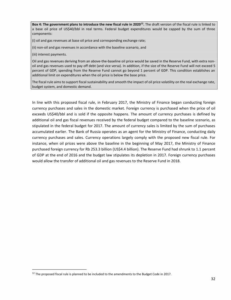
32

Box 4: The government plans to introduce the new fiscal rule in 202012. The draft version of the fiscal ruIe is linked to a base oil price of US$40/bbl in real terms. Federal budget expenditures would be capped by the sum of three components:

(i) oil and gas revenues at base oil price and corresponding exchange rate;

(ii) non-oil and gas revenues in accordance with the baseline scenario, and

(iii) interest payments.

Oil and gas revenues deriving from an above-the-baseline oil price would be saved in the Reserve Fund, with extra non-oil and gas revenues used to pay off debt (and vice versa). In addition, if the size of the Reserve Fund will not exceed 5 percent of GDP, spending from the Reserve Fund cannot go beyond 1 percent of GDP. This condition establishes an additional limit on expenditures when the oil price is below the base price.

The fiscal rule aims to support fiscal sustainability and smooth the impact of oil price volatility on the real exchange rate, budget system, and domestic demand.

In line with this proposed fiscal rule, in February 2017, the Ministry of Finance began conducting foreign

currency purchases and sales in the domestic market. Foreign currency is purchased when the price of oil

exceeds US$40/bbl and is sold if the opposite happens. The amount of currency purchases is defined by

additional oil and gas fiscal revenues received by the federal budget compared to the baseline scenario, as

stipulated in the federal budget for 2017. The amount of currency sales is limited by the sum of purchases

accumulated earlier. The Bank of Russia operates as an agent for the Ministry of Finance, conducting daily

currency purchases and sales. Currency operations largely comply with the proposed new fiscal rule. For

instance, when oil prices were above the baseline in the beginning of May 2017, the Ministry of Finance

purchased foreign currency for Rb 253.3 billion (US$4.4 billion). The Reserve Fund had shrunk to 1.1 percent

of GDP at the end of 2016 and the budget law stipulates its depletion in 2017. Foreign currency purchases

would allow the transfer of additional oil and gas revenues to the Reserve Fund in 2018.

12 The proposed fiscal rule is planned to be included to the amendments to the Budget Code in 2017.

33

Part 2. The outlook for three years: growth prospects are

modest

A moderate recovery of the global economy is expected for 2017, on the back of continued solid growth by

commodity importers and a pickup in commodity exporters during the year. Russia is heading toward a

moderate growth rate over the 2017-to-2019 period (between 1.3% and 1.4%), supported by rising oil prices

and macroeconomic stability.

34

Global growth is expected to recover, but with downside risks. After the divergence of growth in 2015-16 for commodity exporters and commodity importers, global growth is projected to pick up to 2.7 percent in 2017 with broad-based support. In advanced economies, emerging and developing economies, commodity importers, and commodity exporters, growth is expected to accelerate. It will be driven by the bottoming out of investment, strengthening demand from advanced economies, and a modest upturn in commodity prices. Nevertheless, the expected recovery in commodity exporters will be weaker than expected, reflecting longer-than-expected adjustments to low commodity prices in some countries. China’s slowdown is expected to weigh down on commodity importers’ acceleration. In 2018-19, its growth is expected to strengthen to 2.9 percent. However, risks to the outlook are tilted to downside. While the widespread adoption of trade protectionist measures remains a tail risk in the presence of a complex value chain integration, policy uncertainty, including geopolitical risks, has been elevated since the start of 2017. Negative events can weigh on confidence, investment and growth. They can lead to the repricing of risk, which could lead to the sudden tightening of financial conditions for emerging and developing economies.

Crude oil prices remain projected to average $55/bbl in 2017, an increase of 29 percent from last year, and

$60/bbl and $61.5/bbl in 2018 and 2019 respectively13. The oil price increase in 2017 reflects rising oil

demand and falling stocks and assumes an extension of the OPEC/non-OPEC agreement. Prices are projected

to increase to $60/bbl in 2018 as the market regains balance, with shale production limiting larger price gains.

There are significant risks to the oil price forecast. On the upside, stronger demand and greater compliance

by OPEC/non-OPEC producers could accelerate rebalancing, as could supply outages among major exporters

(e.g., Libya, Nigeria, and Venezuela). OPEC policy decisions to expand production cuts could also support

higher prices, as could rising production costs. Downside price risks include weaker compliance with the OPEC

agreement. Rising output from Libya and Nigeria could delay rebalancing, as could slower demand growth. A

faster-than-expected rise in U.S. shale oil production — from further efficiency gains and increased

profitability stemming from potentially lower taxes — could also affect the supply balance. Box 5 discusses

the expected evolution of the Russian oil sector, which so far has taken external headwinds well.

13 The World Bank oil price is an average of three prices (Brent, WTI and Dubai oil prices). The equivalent Ural oil prices (produced

by Russia) are $53.8/bbl in 2017, $58.7/bbl in 2018, and $60.2/bbl in 2019.

Box 5: The Russian oil sector: Increasing production and exports despite headwinds

Russia, the world’s third-largest oil producer after the United States and Saudi Arabia, accounts for over 12 percent of global oil supplies (Figure B5-1). It exports nearly 8 million barrels per day (mb/d), only marginally less than Saudi Arabia’s oil exports (by contrast, the United States imports around 12 mb/d). Russia accounts for a little over 3 percent of global consumption (Figure B5-2), and Russian oil consumption has been relatively stable during the past two decades at around 3 mb/d. Thus, all growth in production goes for exports. Oil and oil products accounted for about 40 percent of Russian merchandise exports in 2015. Oil is also the largest source of tax revenue to the Russian economy.

Russian oil consumption, which had been relatively stable at 2.7 mb/d during 1996-2010, began increasing and reached 3.3 mb/d in 2014. However, the recession, along with economic sanctions, exerted downward pressure on domestic oil consumption in 2015.Russian oil production still increased during the past 2 years by 0.19 mb/d in 2015 and 0.25 mb/d in 2016 and reached a record 11.34 mb/d in 2016.

35

Figure B5-1: Russia was the third-largest oil producer in 2015

Figure B5-2: Russia accounted for only 3 percent of

global oil consumption in 2015

A further, (though marginal) increase in Russian oil production is also expected in 2017, but the larger cuts in production will decelerate the production growth. According to the International Energy Agency (IEA), production growth reflected higher production by small- and medium-size producers (including Gazpromneft, Novatek, Tatneft, Russneft, and Bashneft) as well as deceleration in decline rates across mature fields. Such growth was a result of investment in upstream activity thanks to the ruble devaluation, lower tax rates, and lower input costs. Total oil production is expected to increase to 11.38 mb/d in 2017 and peak at 11.54 mb/d in 2018, as new projects (including Lukoil’s Filanovskoe, Gazpromneft/Russneft’s Messoyakha, Gazpromneft’s Novoport, and Russneft’s Suzunskoe) will more than offset brownfield declines. Production is projected to decline marginally thereafter (Figure B5-3).

In late 2016, Russia, along with Azerbaijan, Kazakhstan, Mexico, and Oman, agreed to join OPEC on production cuts to ease a supply glut and eventually support prices. Russia agreed to a 0.3 mb/d cut, beginning in January 2017 (OPEC and non-OPEC producers agreed to cut 1.2 mb/d and 0.56 mb/d, respectively). Russia’s cuts, which were expected to be gradual, were calculated over October 2016 production levels of 11.6 mb/d. Russia’s compliance was at 40 percent in January and February, increasing to 58 percent in March (or 0.174 mb/d) and 78 percent in April (Figure B5-4). Whether the agreement will be extended to the second half of 2017 will be decided during the May 25 OPEC meeting. Russian officials have expressed public support for a likely extension.

Figure B5-3: Russian oil production has been increasing to record levels

Figure B5-4: Russian compliance to agreed cuts is

increasing

0 5 10 15 20

Indonesia

Mexico

Iran

Canada

Germany

Korea

Russia

Brazil

Saudi Arabia

Japan

India

China

United States

Source: BP Statistical Reviewmb/d

-

2

4

6

8

10

12

1985 1988 1991 1994 1997 2000 2003 2006 2009 2012 2015 2018 2021

Consumption Exports

Source: International Energy Agency.Note: Exports have been calculated as production minus consumption. Shaded area denotes IEA forecasts.

mb/d

30%

40%

50%

60%

January February March April

Source: International Energy Agency

Percent

36

Consistent with our projections in the

previous Russia Economic Report (November

2016), the Russian economy is expected to

grow from 2017 onwards. The positive terms-

of-trade effect, coupled with more stable

macroeconomic conditions, are expected to

positively influence consumer and investor

sentiment, leading to a recovery of domestic

demand and modest economic growth in

2017-19. The growth estimate for 2017 has

been revised from 1.5 percent to 1.3 percent

largely because of the higher base of effect14.

Growth rates for 2018 and 2019 are expected

at 1.4 percent (Figure 36).

Supported by growth in real wages in the private sector, consumption is expected to drive growth in 2017-

2019. We expect headline inflation to continue moderating, falling slightly below 4 percent in the end of 2017

and stabilizing around 4 percent in 2018-2019. Lower inflation will support real wages that will be the main

source of real income growth, as pensions will be indexed with the inflation rate. As the economy recovers,

improving consumer sentiment, growing real wages, and improved credit conditions are all expected to lead

to a growth in private consumption of 1.8 percent in 2017, and 2.5 percent in 2018 and 201915 (Table 3).

Table 3: Projected GDP growth by component, percent, y/y and contribution to GDP growth, pp

Growth, y/y, percent Contribution to growth, pp

2017 2018 2019 2017 2018 2019

GDP 1.3 1.4 1.4 1.3 1.4 1.4

Consumption 1.1 1.6 1.6 0.7 1.0 1.1

Gross capital

formation 8.0 1.5 1.1 1.5 0.3 0.2

Gross fixed capital

formation 2.0 2.5 3.5 0.4 0.5 0.7

Export 2.0 2.3 2.5 0.6 0.7 0.8

Import 10.0 4.0 4.0 -1.5 -0.6 -0.7

Source: World Bank staff calculations.

Investment demand is expected to pick up in 2017-2019. Given a massive inventory destocking in 2015 and

a recovering economy, we expect businesses to renew their stocks in 2017, boosting import growth to 10

percent y/y and providing support to some manufacturing sectors. We expect a pick-up in fixed capital

investment growth in 2017 to 2.0 percent due to macro stabilization, improved investors’ sentiment and a

stronger ruble; together, these factors could help companies realize some deferred demand for equipment.

The 2018 soccer World Cup could further support public investment. Fixed capital investment growth is

expected to accelerate to 2.5 percent and 3.5 percent in 2018 and 2019 respectively, as economic policy

14 Rosstat revised SNA data for 2015 and 2016. As a result, GDP contraction in 2015 was lower than it was recorded previously (-2.8 percent compared to -3.7 percent before). 2016 quarterly growth was reviewed upwards so that expected fall of GDP by 0.6 percent was changed to 0.2 percent. 15 Growth in consumption is tempered because of the planned fiscal consolidation which will limit government capacity to support consumption through real increases in public sector wages.

Figure 36: The economy is expected to grow in 2017-2019 at a

modest rate (real GDP growth, percent)

Source: Rosstat, World Bank.

37

uncertainty subsides and external demand further improves. The lower cost of credit will also support the

growth of fixed capital investment in 2018 and 2019. As we expect restocking to happen mostly in 2017, the

investment-demand contribution to growth will contract in 2018 and 2019, compared to 2017.

The contribution of net exports to growth is expected to be negative in 2017 and slightly positive in 2018-

2019. With marginally slowing growth in the Euro Area and Japan, a modest pick-up in growth in the US and

a gradual slow-down China, we expect exports to grow by 2 percent in 2017. The export growth rate will

slightly increase in 2018 and 2019 on the back of higher global growth. From a low base in 2016, and

supported by an improvement in domestic demand (inventory restocking and deferred demand for

investment imports), imports are expected to continue recovering in 2017 and beyond. In 2017, we expect

import growth to outstrip growth in exports, thus leading to an overall negative contribution of net exports.

In 2018-2019, the net exports contribution to GDP growth is expected to be slightly positive.

Higher oil prices will support the current account, which is expected to increase to 2.9 percent of GDP in

2017 from 1.9 percent of GDP in 2016. A further gradual increase in imports, including services imports, is

expected to slightly weaken the current account in 2018 and 2019 (Table 4).

Table 4: Major macroeconomic indicators

2016 2017 2018 2019

Oil price (US$ per barrel, WB average) 43.3 55 60 61.5

World economy growth, percent 2.3 2.7 2.9 2.9

GDP growth, percent -0.2 1.3 1.4 1.4

Consumption growth, percent -3.5 1.1 1.6 1.6

Gross capital formation growth, percent 1.5 8.0 1.5 1.1

General government balance, percent of GDP -3.5 -1.8 -0.5 0.3

Current account (US$ billions) 25.0 45.7 46.0 45.9

Current account, percent of GDP 1.9 2.9 2.7 2.6

Capital and financial account (US$ billions) -15.7 -31.7 -23.3 -21.3

Capital and financial account, percent of GDP -1.2 -2.0 -1.4 -1.2

CPI inflation (average) 7.1 4.1 4.0 4.0 Source: World Bank staff calculations.

38

Growth projections remain sensitive to oil prices.

A simulated decrease of 15 percent in oil prices

reduces growth to 1 percent in 2017 and 1.2

percent for 2018 and 2019. A simulated rise of 15

percent in oil prices increases growth to 1.6

percent for 2017 and 1.8 percent for 2018 and

2019 (Figure 37). Despite policy efforts to reduce

sensitivity, oil price volatility would still affect

consumer and producer sentiment. We expect a

slightly higher response of the economy on the

upper oil price-variation due to improved investor

sentiment.

The poverty rate is expected to decrease because

of decelerated inflation and a recovery in household incomes and consumption. In the baseline scenario,

the poverty headcount is projected to decline in 2017 to 13 percent from 13.5 percent in 2016, and to

continue declining to 12.3 and 11.6 percent in 2018 and 2019 respectively (Figure 38). Household

consumption and incomes will also be supported by an increase in pensions that were indexed by end-year

inflation and are likely to increase slightly in real terms during 2017. Figure 38 also shows the sensitivity of

poverty projections to the minus/plus 15-percent change in oil prices (scenarios 2 and 3) compared to the

baseline.

Figure 38: The poverty headcount is likely to decline in 2017 and further (in percent)

Source: Rosstat, World Bank staff calculations.

The prognosis

Overall, the short-term prognosis for the Russian economy is favorable, with projected growth rates between

1.3 to 1.4 percent in the forecasting period of 2017-2019. Among other factors for this recovery, maintaining

macro stability is a central contributing one. Moreover, a return to the three-year federal budget law and

introduction of the updated fiscal rule is expected to further increase economic predictability. The projected

improvement in private consumption is also expected to support economic activity in the non-tradable and

tradable parts of the economy (Table 5).

0.406

0.408

0.410

0.412

0.414

0.416

0.418

0.420

0.422

10

11

11

12

12

13

13

14

14

2009 2010 2011 2012 2013 2014 2015 2016 2017 2018 2019Poverty rate, % Scenario 1 (baseline) Scenario 2 (lower-bound)

Figure 37: Growth projections remain sensitive to oil prices (GDP growth, percent)

Source: World Bank staff calculations.

39

Table 5: Recovery is expected to be broad-based: projected growth by sector

2016 2017 2018 2019

Agriculture 3.6 1.2 1.7 1.7

Industrial production 1 1.2 1.6 1.3

Services -0.9 1.3 1.3 1.4

Source: WB staff calculations.

Agriculture, in particular, is expected to benefit. After high growth in 2016 on the back of a good crop, we

expect growth to slow down in 2017-2019. Previous years’ investment in the dairy sector would support this

growth. While a detailed analysis of the agricultural sector is beyond the scope of this report, Box 2 discusses

issues germane to productivity in two agricultural sub-sectors: pork production and dairy farming.

Box 6: Productivity in pork production and dairy arming: revenues, profitability and labor productivity increase, but opportunities remain to improve land and capital productivity.

This box examines selected factors, namely the productivity and profitability of farms, to interpret drivers and bottlenecks for agriculture-sector performance in Russia. The Ruslana database was used to assess the performance of farms in two priority livestock sectors: pork production and dairy farming. These are priority sectors for agricultural development and have been the focus of much policy attention since the 2000s. The two samples paint a representative picture of the performance of small, medium and large agro-enterprises.

Both sectors – pork production and dairy farming – have demonstrated significant growth since 2007. Revenue growth in real terms between 2007 and 2016 was more than 200 percent for dairy and more than 1,000 percent for the pork industry. The largest growth in revenues was reported by large agro-enterprises, with averages of 40 percent per annum in the dairy sector and 150-200 percent per annum in the pork sector. More than the capital-intensive dairy sector, three-digit growth rates in revenues are transforming the pork industry, which is now being dominated by medium-to-large enterprises.

Profitability in the dairy and pork sectors has also been growing, although the pace of growth has been slowing down since 2007. The main drivers of profitability in both sectors are relatively high domestic prices for both pork and milk (Figures B6-1 and 2) and relatively low domestic prices for feed, which makes up to 60 percent of production costs. So far, Russian farming enterprises enjoy favorable domestic market conditions characterized by protection from import competition and higher prices.

In addition to their favorable domestic market situation, pork and dairy farms have also demonstrated advances in productivity. A separate analysis of economy-wide labor productivity in the agro-food sector (partial TFP analysis) shows that labor productivity has been increasing in the past 10-12 years, though with a small growth rate of 1.5 percent per year on average. Productivity increases are fueled by major technological advances that the agro-food sector carried out in the last decade, notably imports of new technologies and improved genetics, animal health conditions and management methods.

However, at the farm-enterprise level, results for dairy vary depending on the farm size (Figure B6-3). Medium and large dairy farms reported average annual labor productivity growth of 3.3 to 3.6 times over the past 10 years, with large companies reporting labor productivity growth in the order of 10 times during this period. Small enterprises reported a productivity decline, and considering the sizeable contribution of small and medium enterprises in the dairy production, their results weighed on overall sector productivity.

The main drivers of profitability in both sectors are relatively high domestic prices for both pork and milk

40

It is worth emphasizing, however, that though Russia is expected to grow modestly in the short-term future,

its longer-term growth prospects remained constrained by low Total Factor Productivity (TFP) growth. Box 7

Figure B6-1: Pork Prices (in rubles)

Source: Ruslana database.

Figure B6-2: Milk Prices (in rubles)

Source: Ruslana database.

Figure B6-3: Pork Prices (in rubles)

Source: Ruslana database.

While these are encouraging developments for the pork production and dairy sectors, compared to similar farms in Europe and North America, non-feed costs (overhead, depreciation, paid labor and others) – which are around 40-50 percent of total costs – are higher on Russian farms. Both land and capital productivity per unit of milk produced is low in Russia compared with European and North American comparator farms, suggesting opportunities for improvement of land management and capital intensification.

Labor productivity is relatively low compared with international competitors but so are salaries – thus labor costs are presently not higher than in Western farms. However, with improvements in the overall economic development and increasing wage levels, the agriculture sector must improve labor productivity if it wants to remain competitive with other sectors. In this context, the lack of skilled labor is also a profound disadvantage that needs to be addressed.

41

discusses various methods and measures of TFP growth in Russia, all which yield the same conclusion: TFP

growth in Russia is low and declining.

Box 7: Russia’s potential GDP and TFP revisited: declining productivity trends

Total factor productivity (TFP) is a measure of efficiency that is notoriously difficult to calculate. Simply put, it is the portion of output that cannot be explained by the traditional inputs of capital, labor and land. Its level is the measurement of how efficiently the inputs are utilized, and it depends critically on the accuracy and availability of data and of the behavioral forms that translate inputs into outputs.

Traditionally, TFP is estimated as the residual explanation of GDP growth after accounting for the contribution of the factors of production: capital, labor (both unskilled and skilled) and land. The relative shares with which these inputs contribute to growth are determined by the wage bill, the cost of capital, the returns to education and land rents. Often, data on factor quantities and prices are unavailable and need to be estimated; as a result, the residual, or TFP, is subject to measurement error.

For example, the factor shares are often estimated using volume data (the number of hours worked, the number of employees and the amount of capital stock). This also requires various assumptions regarding the functional form of the economy-wide production function. The production function that is most commonly used in this type of exercise is the Cobb-Douglas production function, which assumes that labor and capital are used in fixed proportion in the production of goods. This result can be tested by nesting the Cobb-Douglas function into a constant elasticity-of-substitution (CES) function. Depending on the estimated coefficients, the factors of production may be complements, in which case an increase of labor in production will also result in an increase in capital, while substitution effects imply that using more labor in production will result in a reduction of capital.16 The residual measure that is often labelled as TFP is, then, a catchall for all efficiency, technological effects and even measurement errors.

The economy of Russia has been hit by deep structural changes over the last couple of decades. The transition to a market-based economy and changes in population and in its natural-resource base imply large shifts in TFP. Russia produces significant amounts of oil and gas, which contributes substantially to its output. The production function must therefore be augmented for resources to avoid possible bias in measuring TFP. The share of resources in output is calculated by multiplying the rents of oil and gas with the production of oil and gas and expressing it as a share of GDP.

Another source that contributes to TFP is structural changes in employment mobility and human capital. This exercise assumes that skilled workers (skills are determined by education) are more efficient. Furthermore, we think of labor productivity growth as the contribution of within sectoral contributions (such as an increase in research and development) and between sectoral contributions that account for shifts in employment shares between sectors. If the employment share has increased in a productive sector, then structural change has contributed to productivity growth. In Russia, the share of employment in industry has declined since 2000, while the share of service employment has increased. A second measure of TFP is constructed by controlling for the number of years of education and the labor share of each industry (see McMillan et al. [2014] and Burns (2016]). The number of years of education is obtained from the Barro and Lee (2013) data set. Controlling for structural change and skills nets out more effects from TFP and arguably allows us to get closer to an accurate interpretation of TFP.

Three estimates of TFP are presented in this box: (i) The CES production function without oil that uses only capital and labor as inputs; (ii) the estimate derived from a Cobb-Douglas production function and netting out the contribution of labor share changes from growth (here referred to as structural change) and (iii) one estimated from a Cobb-Douglas production function, but that includes hydrocarbon resources and education. The three methodologies provide useful comparisons in understanding TFP where (i) is a reference point to compare TFP growth by netting out distinctly different aspects of growth using (ii) and (iii). To calculate potential GDP, we follow Burns (2016) by smoothing TFP with an HP-filter and assume that capital is fully utilized.

Figure B7-1 decomposes potential GDP into its components using (iii). The transition away from a centrally planned economy to a market-based economy is captured by the change in capital’s contribution to potential GDP growth in

16 Rough estimates using a CES specification for Russia suggest that the production function is a Cobb-Douglas.

42

the late 1990s. The role of TFP in potential GDP growth started moderating in the early 2000s, while the labor force and the resources started contributing more to growth towards the end of the sample. The contribution of TFP to potential GDP since the global financial crisis of 2008/09 has almost disappeared, highlighting the constraints placed on productivity from the adverse effects of the crisis. Figure B7-2 summarizes the different TFP outcomes from the three methodologies. The estimate of TFP using (i) above is labelled CES and strikingly shows how large TFP was in the late 90’s controlling only for labor and capital. The magnitudes of TFP are markedly different in the late 1990s, illustrating the effects of leaving out oil and education (iii) and structural change (ii). More importantly, ignoring the effects of resources and education would have implied that TFP growth was moderating sharply, whereas the other measures suggest a more gradual moderation in TFP growth.

None of the approaches is necessarily superior to the other. Each methodology strips some component from TFP. For example, TFP adjusted for skills and resources is much lower in the initial periods compared to the other measures. More importantly, the decline in TFP is also less marked when adjusting for skills and resources. Adding the resources reduces capital’s share in measuring TFP and seems to be an important factor in explaining the initial differences.

However, regardless of the method used, all have the following in common: TFP growth across all measures has been declining over time, underscoring the challenge of addressing declining productivity growth in Russia.

Figure B7-1: Decomposing potential GDP growth Figure B7-2: TFP growth according to different

measures

-2

0

2

4

6

8

10

12

1998 2000 2002 2004 2006 2008 2010 2012 2014 2016

CES

Structural change

Education and resources

% change

Source: Authors’ own calculations using WDI, Rosstat and

ILO.

Source: Authors’ own calculations using WDI, Rosstat and

ILO.

With low TFP growth and a declining labor force, potential output growth is modest at best (around 1 to 1.5

percent of GDP), thus limiting GDP recovery growth rates. And as discussed in earlier sections, over the past

nine years, unit labor costs in Russia have risen much faster than in any other OECD country, weakening the

competitiveness of the Russian economy. Addressing these deeper structural challenges will have the sought-

after payoff of inclusive, sustainable and fast-paced growth.

-6

-4

-2

0

2

4

6

8

10

1998 2000 2002 2004 2006 2008 2010 2012 2014 2016

TFP

K

LF

LFPR

EDUC

OIL

EMP Ratio

Potential GDP

% contribution

43

Part 3. Russian regions and their responses during the crisis

years

This part analyzes subnational fiscal trends in Russia in the context of an overall slowing of economic growth

and falling oil prices since 2014. It discusses how Russian regions fared during the crisis and examines their

fiscal prospects, focusing particularly on whether their crisis measures – driven by spending cuts – are

sustainable over the medium term.

44

Russia has a complex structure of subnational government. At the top level, the country is divided into over 80 federal subjects, termed oblasts and federal cities. Territorial subdivisions also include krais (administrative territories), republics, autonomous okrugs (territorial divisions), and autonomous oblasts. The administrative units are grouped into eight federal districts, each headed by a presidential plenipotentiary appointed by, and representing, the President of the Russian Federation. The envoy monitors the performance of the regions in each federal district. Hereafter, all these top-level geographical units will be referred to as “regions.17”

The territory of each regional government is in turn divided into what might be termed “first-tier municipalities.” These consist of large cities (formerly known as cities of oblast subordination) and rural raions (districts); the latter contain a variety of forms of small towns and village governments, which this report will refer to collectively as second-tier municipalities. There are more than 2,000 first-tier municipalities comprising more than 500 cities and more than 1,800 raions; and there are more than 20,000 second-tier municipalities, comprising more than 1,600 townships and more than 18,000 rural communities.18

Under the current legislation, all municipalities (including rural settlements with small populations) are required to establish local governments, employ municipal office staff, formulate and execute budgets, and conduct an independent debt policy. The law assigns a set of expenditure responsibilities to each tier of municipal government (See Box 8). In practice, municipalities tend to be highly dependent on their respective regional governments. They have limited taxing powers and depend on transfers and shared taxes from their respective regions; as detailed below, the only major federally designated source of revenue for municipal governments is a share of the personal income tax (PIT). As a result, the municipalities tend to function as spending agents of their respective regions, rather than as independent tiers of government.

17 IMF Article IV Consultation, July 2010. 18 The federal cities are also divided into municipalities. Recent (2014) legislation permits other large cities to do the same.

Box 8: Russian federalism in the international context

In aggregate terms, the degree of fiscal decentralization in Russia is similar to that of other large, middle-to-high-income federal countries. The first figure below shows the share of total general government expenditures that are accounted for by subnational governments in Canada, the U.S., Australia, Russia, Brazil, and Germany. As shown, Russia is not unusual. It is less decentralized by this measure than the U.S. or Canada but roughly on par with the other three comparators. Another way to measure decentralization is to look at the size of subnational government as a share of GDP. Again, Russian subnational governments are not as large as those in Canada, but they are roughly on par with those in the U.S., Germany, and Brazil. Interestingly, the split in Russia between spending at the regional level and at the local (municipal) level is also similar to that in the U.S., Brazil, and Germany. A third approach is to calculate the percentage of subnational revenues that are derived from own-source revenues. By this measure, Russia is again fairly typical of large federations. Regional governments in Russia derive 80 percent of their income from own-source revenues (including shared taxes, distributed on the basis of origin). This is similar to the proportions in Germany (84 %); Canada (81%); and Brazil and the US (both 77 %). (Note that these figures refer only to regional governments. Local/municipal governments in Russia and other federations derive a larger proportion of their revenues from transfers from their respective regional governments.)

The degree of fiscal decentralization in Russia is similar to that of other large, middle-to-high-income federal countries

Figure B8-1: Subnational spending, (percent of general government)

Figure B8-2: Subnational spending, (percent of GDP)

45

Functions

The functions of each tier of subnational government are set out in federal legislation. Subnational functions are broad-ranging. They include the provision of social assistance, education (kindergarten and grades 1-11), and the operation of health care facilities (although general hospitals are largely funded by the regional divisions of the national health insurance fund and are managed at the federal level). In the infrastructure sectors, their responsibilities include regional and intra-city roads. Subnational governments are also responsible for the provision of public utilities (e.g., district heating and water supply) and public transportation. In total, subnational governments account for about one-third of total government expenditure.19

As shown in Figure 3920, the social sectors — education, social protection and health — together account for just over half of total subnational expenditures. In 2016, education was the largest single functional category (26 percent); followed by transport (20 percent); social protection (17 percent); and health care (13 percent). Social protection expenditures include not only payments to impoverished households but to most old-age pensions.

19 In calculating this percentage, the total is calculated as the sum of federal expenditures, regional and municipal expenditures, and expenditures of federal extra-budgetary funds (the pension fund, social security fund, and the medical insurance fund together with its regional divisions). Due to intergovernmental transfers between these entities, when estimating the shares of each entity, all intergovernmental fiscal transfers are netted out. Thus, for example, subnational spending on hospitals, financed through the national health insurance fund, are not included in ‘subnational expenditures’. 20 Figure 1 shows the consolidated expenditures of all three tiers of subnational government, with transfers from oblasts to raions and from raions to second-tier municipalities netted out.

Source: Federal Treasury of the RF, IMF, and US census of govt. Source: Federal Treasury of the RF, IMF, and US census of govts. Note: data is based on IMF Government Finance Statistics (except US, where it also incorporates data on local finance from the US Census of State and Local Governments). Expenditures by central and provincial government are net of transfer to subordinate levels of government. Provincial government are net of transfer to subordinate levels of government.

Figure 39: Social sectors together account for just over half of total subnational expenditures

Source: Federal Treasury of the RF.

46

Financing

The general budgets of all three tiers of subnational government (regional, and first and second-tier municipal governments) are financed from a combination of shared taxes, exclusive local taxes, own non-tax revenues, and intergovernmental transfers. All taxes are administered by the federal tax service with revenues returned in whole or in part to the jurisdiction in which they were collected. Shared taxes are the largest source of subnational government revenue. Two of them — the personal income tax (PIT) and the corporate income tax (CIT) — accounted for over half (53 percent) of total subnational

revenues in 2016 (Figure 40). Regional governments are allowed to adjust the rate of the CIT within a range of 13.5 to 17 percent. They have no control over the rate of the PIT. The share of exclusive local taxes in the composition of subnational revenues is 23 percent, of which 8

percent is derived from various forms of property tax. By far, the largest form of property tax — accounting

for 68 percent of the total in 2016 — is the corporate asset tax. This is imposed on movable and immovable

property owned by registered companies. Until recently, assessments were based on book values, which

were substantially below market values. With the encouragement of the federal government, regions

are now gradually introducing market values for particular groups of taxpayers. The maximum rate on

the corporate property tax is a substantial 2 percent.

In addition to the tax on corporate assets, there are two other forms of property taxes. The first is on

land. This tax is imposed on both urban and rural plots of land (except forests). Since 2014, land has

been valued based on its cadastral value. Proceeds are retained at the municipal level, and municipal

governments (including the cities of Moscow, St. Petersburg, and Sevastopol) are permitted to set the

rate of the tax, subject to a ceiling of 0.3 percent on agricultural and residential property and 1.5 percent

for land in other uses. The land tax accounts for 20 percent of property tax revenues, although only 2

percent of total subnational revenues.

The second is a tax on buildings. This is imposed on residential and commercial property owned by individuals

(as opposed to corporations). Since 2014, the tax has been assessed based on cadastral values, although these

are often out of date. Proceeds are retained at the municipal level. Municipal governments are permitted to

set the rate of the tax, subject to federal ceilings. The maximum rate of residential properties is extremely low:

0.1 percent. Federal law also permits a long list of exemptions and rate reductions for certain classes of

taxpayers (e.g., pensioners and veterans) and types of property. As a result, the yield of the building tax is

trivial — only 0.36 percent of total subnational revenues.

Then there are the subnational shares of certain excise taxes on alcohol and gasoline. Taken together (with other excise taxes), they account for 7 percent of total subnational revenues. Subnational governments also generate income from a variety of other taxes. Together, these account for about 8 percent of their revenues. The most important one (accounting for a third of the total) is the transport tax. Regions are also entitled to

Figure 40: Shared taxes are the largest source of subnational government revenue

Source: Federal Treasury of the RF.

47

revenues from certain mineral resource extraction taxes, namely the tax on the extraction of common minerals and the tax on “other minerals excluding hydrocarbons.” These taxes are not major revenue sources from an aggregate standpoint but are important in certain regions such as Sakha-Yakutia, a diamond-producing region. Non-tax funding is also significant. Non-tax, own-source revenues are non-trivial; they account for about 7 percent of total revenues. At the same time, transfers from the federal government (i.e., money distributed to regional governments on a basis other than origin) accounted for 16 percent of regional revenues in 2016. The Russian budget code distinguishes three types of transfers: dotacii, subsidii, and subventsii.

Transfers that are not earmarked for specific uses are referred to as dotacii. They account for 42 percent of total federal transfers. The largest dotacii — and the largest single transfer from the federal government to the regional tier of government — is the equalization grant. This grant is designed to raise the per capita budget revenues of poorer regions (those with per capita revenues below the national average) up to a target percentage of the national average. In calculating the equalization target, the 10 richest and 10 poorest regions are excluded. Adjustments are also made to reflect variations in the strength of tax bases among different regions, as well as differences in factors that affect the costs of providing services (for example, labor costs, the cost of living, and population density). The total amount of the transfer is determined endogenously; i.e., the federal government is required to contribute whatever sum is needed to achieve the equalization target. Roughly three-quarters of the regions receive equalization grants.21 In 2016, they accounted for about 78 percent of total dotacii.

Subsidii are federal matching grants. These support a wide range of federal programs, some of which involve capital investments.

The third major category of transfers, subventsii, consists of compensation for functions that subnational governments perform on behalf of the federal government. These include unemployment subsidies, rent subsidies granted to certain categories of federal beneficiaries such as war veterans or victims of radiation catastrophes, benefits paid to blood donors, and the costs of running civil registration offices.

Regional variations in per capita revenues These aggregate figures for Russia conceal substantial variations across regions — both in terms of the levels of aggregate revenues (per capita) and their composition. The table below illustrates the variations in per capita revenues among regions22 (Table 6). The figure for each region includes the own-source revenues of subordinate jurisdictions. Thus, it represents the consolidated per capita revenues of all subnational governments in that region, from the regional government itself to the smallest second-tier municipality. Revenues are expressed in thousands of rubles per capita and include both own-source revenues and transfers from the federal government. In essence, the regions fall into three groups. The first group consists of the eight (generally) sparsely populated oil/gas/gold-producing regions located in the far North and East of the country, mostly in Siberia. The second group consists of the cities of Moscow and St. Petersburg, which receive unusually high own-

21 Starting in 2016, the transfer allocation rules guarantee that regions whose revenues from the equalization transfer are at least 10 percent greater than their other revenues shall receive no less than 90% of the previous year’ amount.

22 The table does not include all regions.

48

source revenues, notably corporate and personal income taxes. Neither derives significant revenue from federal transfers. The third group consists of all the other regions. Only about 10 percent is derived from equalization transfers.23 As a result, variations among individual jurisdictions largely reflect variations in their respective tax bases.

Table 6: Per capita revenues of regions vary widely

Rich naturalresource based regions

88 - Chukotka Autonomous Okrug 555 90 – Yamalo-Nenets Autonomous Okrug

255

61 – Sakhalin oblast 457 38 – Kamchatka Krai 205

84 - Nenets Autonomous Okrug 426

Moscow, Saint Petersburg

73 – Moscow 137 St. Petersburg 86

All others

77 – Altai Republic 79 28 - Vladimir oblast 41

07 – Komi Republic 78 27 – Bryansk oblast 40

19 – Krasnoyarsk Krai 74 63 – Smolensk oblast 40

48 - Moscow oblast 73 52 – Omsk oblast 40

22 – Khabarovsk Krai 68 55 – Penza oblast 36

23 – Amur oblast 64 15 – Chuvash Republic 36

11 – Tatarstan Republic 63 10 - Republic of North Ossetia-Alania 35

78 - Jewish Autonomous Oblast 61 33 – Ivanovo oblast 35

34 – Irkutsk Oblast 53 60 – Saratov oblast 35

80 - Republic of Khakassia 53 04 – Republic of Kabardino-Balkaria 34

14 – Republic of Ingushetia 53 21 – Stavropol Krai 33

57 – Pskov Oblast 41 03 – Republic of Dagestan 30 Source: Federal Treasury of the RF.

Fiscal Performance

23 The remaining 15 percent is derived from subsidii, subventsii, and other federal transfers.

49

At an aggregate level, subnational governments seem to be weathering the ongoing slowdown in the economy fairly well. As figure 41 shows, the aggregate subnational balance reached its nadir in 2013 (at 0.9 percent of GDP), just as the slowdown in the economy was beginning (Russia’s GDP was still growing in 2013, albeit at an anemic 1.3 percent). In 2014, the GDP growth rate shrank to 0.7 percent. In 2015 and 2016, the economy contracted by 2.8 percent and 0.2 percent respectively. Still, the aggregate subnational balance improved over this period, with the deficit declining from 0.6 percent of GDP in 2014 to zero percent of GDP in 2016. As a percentage of revenues, the consolidated subnational deficit declined from 8 percent to only 0.1 percent. And as Box 9 illustrates, the good aggregate fiscal performance of subnational governments is not affecting the federal government much. This is because of the hard line taken by the federal government in drastically reducing transfers to regions by as much as 22 percent in real terms between 2013 and 2016.

Russia’s economic slowdown triggered a fiscal adjustment at the subnational level; as aggregate subnational revenues declined significantly between 2013-16 (9 percent in real terms), the adjustment occurred mostly on the expenditure side (figure 42). As a group, subnational governments managed to cut expenditures by 16 percent in real terms between 2013 and 2016 — 7 percentage points more than the cuts in revenues. The largest cuts, in absolute terms, were in education (figure 43). Total spending on this sector fell 18 percent in real terms between 2013 and 2016 (increasing only 9 percent in nominal terms). Spending on health declined 23 percent over the period, although this was partly offset by an expansion in the number of facilities covered by the HIF. There were even sharp cuts in spending on social protection, which fell 6 percent in real terms over the period. It should be noted that regional governments have considerable discretion in designing their own social-assistance programs. As long as federal guidelines are respected,

Figure 41: Trends in subnational deficits: subnational governments seem to be weathering the ongoing slowdown in the economy fairly well

Source: Federal Treasury of the RF.

Box 9: Subnational fiscal performance is not affecting the federal government much

At present, the fiscal difficulties of subnational governments are not directly affecting the federal government budget. This is because the federal government is taking a hard line: between 2013 and 2016, transfers from the federal government fell 22 percent in real terms.

The federal government does have some exposure to subnational loan defaults. As of end-2016, federal loans to subnational governments totaled Rb 1 trillion. Subnational governments also have a significant level of debt to commercial banks. But the level of debt in most jurisdictions (including the largest ones) appears to be manageable.

On the surface, therefore, the outlook from the federal government’s perspective is fairly good: subnationals are responding to the declines in revenues by cutting expenditures, rather than by running up debt or demanding federal bailouts (at least not successfully). One should not be too sanguine, however. Subnational governments may be engaging in fiscal maneuvers that are not evident in the data: e.g., accumulating arrears and unfunded obligations. Moreover, it is not clear how long the federal government can continue relying on expenditure cuts at the subnational level before the social and political consequences become so great that it is forced to step in.

50

regional governments may cut benefits to fit their own budget constraints, and they may have responded to the decline in their overall revenues by doing exactly that. In addition to the cuts in social spending, subnational governments also made substantial reductions in infrastructure spending; in particular, cuts in the transport sector accounted for 14 percent (in real terms) between 2013 and 2016. Spending in the housing and communal services sector fell even further, by 22 percent.

Figure 42: Trends in subnational revenues: aggregate subnational revenues declined significantly between

2013-16

Figure 43: Trends in subnational expenditures: the adjustment occurred mostly on the expenditure side

Source: Federal Treasury of the RF. Source: Federal Treasury of the RF.

While the aggregate subnational deficit in 2016 was close to zero (0.01 percent of GDP and 0.1 percent of consolidated revenues), there were still signs of fiscal distress in some jurisdictions. Eight jurisdictions had deficits of over 10 percent, measured as a share of their own revenues. The Republic of Khakassia, the Yamalo-Nenets Autonomous Okrug, and the Kostromskaya oblast topped the list, with deficits of 27 percent, 23 percent, and 15 percent, respectively.24

Subnational deficits, particularly during the first economic crisis (2009) and the more recent nadir of 2013, have resulted in growing levels of subnational debt. As shown in Figure 44, the level of subnational debt peaked (in constant terms) in 2014, but it has since stabilized. Subnational debt totaled Rb 2,353 billion at the end of 2016. This was equal to 35 percent of subnational discretionary25 revenues and 2.7 percent of GDP. While the aggregate level of subnational debt (35 percent) is not large, relative to revenues, some individual regional governments are highly indebted. Over half of them have debt-to-revenue ratios in excess of 50 percent. The carrying costs of this debt is generally low, but its short-term nature represents a significant rollover risk in some jurisdictions.

A significant part of subnational debt (39 percent) takes the form of short-term loans from commercial banks.26 Commercial banks are increasingly reluctant to roll over their existing loans to subnational

24 However, these regions do not violate the 15 percent deficit restrictions imposed by the Budget Code because these restrictions do not apply to deficits covered by federal loans. 25 Discretionary revenues are defined as total own-source revenues (including shared taxes) plus unconditional grants. 26 These banks are not, strictly speaking, private. Commercial bank lending financing of subnational governments is dominated by two state-controlled banks: Sberbank and VTB.

Figure 44: Short-term loans account for over one-third of the subnational debt

Source: Federal Treasury of the RF.

51

governments and charge high interest rates if they are willing to roll them over at all. In response, the federal government has stepped in. Federal loans now account for one-third of subnational debt. Box 10 describes the tight system of federal controls over subnational deficits.

Prognosis

While subnational governments have, so far, successfully adjusted to the recent economic downturn, it is not clear how sustainable this adjustment will be — and what its implications are for the services that subnational governments provide. Persistent cuts in spending on education will make it difficult to attract and retain qualified teachers, eventually resulting in declining levels of student learning. Cuts in spending on social protection will result in increased levels of poverty, not only among the economically disadvantaged but also among most pensioners. Cuts in transport will lead to increasing traffic congestion and wear and tear on vehicles. Cuts in spending on utilities will result in more erratic levels of service.

Box 10: Federal controls over subnational deficits

At present, subnational deficits are controlled by a tight system of regulations set out in the Budget Code. The code specifies three types of ceilings.

The first refers explicitly to deficits. Budget deficits of regional governments may not exceed 15 percent of annual revenues. For municipalities, the ceiling is 10 percent. In both cases, the calculation of revenues excludes intergovernmental transfers. In the case of municipalities, it also excludes revenues from shared regional taxes. Even tighter limits are placed on regions that are highly dependent on transfers. For regional governments that derived more than 40 percent of revenues from transfers during two of the three previous years, the deficit may not exceed 10 percent of revenues, excluding intergovernmental transfers. For municipalities that derived more than 50 percent of revenues from transfers, deficits may not exceed 5 percent of revenues (again, excluding transfers and shared regional taxes).

The second and third ceilings control borrowing — i.e., the source of financing for deficits. In particular, the second ceiling refers to debt stocks. The Budget Code stipulates that the outstanding debt of a region or municipality may not exceed 100 percent of its annual revenues, excluding intergovernmental transfers. For transfer-dependent regions and municipalities, the ceiling is 50 percent. The third ceiling refers to debt service. The Budget Code stipulates that the debt service of a region or municipality may not exceed 15 percent of expenditures of the relevant year.

In theory, these restrictions should act as a brake on subnational deficits. With explicit ceilings on the size of deficits and limited access to debt, subnational governments should be compelled to finance their expenditures from recurrent revenues supplemented by the sale of assets. But there are loopholes in the regulations, which are being addressed. For example, until 2017, federal refinancing loans were exempted from the debt ceilings. However, subnational governments may also accumulate debt in ways that evade tighter regulations. These can take the form of arrears to their employees and suppliers, including public utilities. These arrears can be accumulated by subnational governments themselves or by enterprises they own. The scale of these liabilities cannot be determined, as such information is not collected and published on a regular basis by the federal government or by the regions.

52

SHORT-TERM MEASURES

Revenues In theory, the federal government could provide support — for instance, by increasing transfers to subnational governments. However, with the federal government itself fiscally constrained, there is a need to look for additional measures.

On the revenue side, regional governments could raise the CIT rate to the maximum 17 percent and refrain from granting exemptions and tax reductions to individual firms in the future. Given the importance of the CIT, this could have a significant impact on revenues, particularly in the more industrial and urbanized regions. The federal government, for its part, could also increase the personal income tax rate, which as noted earlier, is shared with subnationals. Subnational governments could increase the yields of other taxes. For example, regional governments could accelerate the shift from book value to market value as the basis for assessing the tax on corporate property. They could also transition more quickly to market values as the basis for assessing the land tax and the building tax. The first of these measures could have a significant impact on regional revenues. For the latter measures to have an impact, the federal government would have to raise the ceiling on the maximum rates of the land and building taxes. Expenditures On the expenditure side, subnational governments could continue to pursue what appears to be their current strategy — cutting capital expenditures and restraining the wage bill.27 This is a common adjustment strategy for both central and local governments in much of the region. As a short-term measure, it can work well. On the capital spending side, new starts on capital works can be readily postponed. But suspending ongoing capital works is more problematic, as half-completed works can fall into ruin long before funding becomes available to complete them. Overall, the fiscal impact of cutting capital spending is not likely to be large. This is because capital spending represents only a small proportion of total subnational spending (in Russia, the proportion in 2015 was about 10 percent). Cutting the wage bill is likely to have a much larger effect, due to the large proportion of subnational spending that is (presumably) devoted to salaries. In principle, there are two immediate ways to cut wage spending. The first is by freezing nominal wages. This can have a substantial and immediate impact. With the inflation target of 4 percent, which the central bank strives to reach by end 2017, a freeze on current nominal wages would reduce the wage bill by a proportionate percentage per year in real terms. This could, of course, run afoul of the federal directive requiring the salaries of certain professions, such as teachers and health workers, to equal the prevailing wage in each region. But if regional wages are also falling, even this obstacle might not have much effect.28 The second technique is to reduce staffing numbers. Efforts to do so on a large scale can be difficult. In most European countries, confirmed civil service employees are typically protected from dismissal except for cause (public-sector unions also play a role in restraining downsizing). A more palatable approach is to freeze new

27 Direct evidence of reductions in the wage bill is not available as subnational expenditures in labor-intensive sectors, such as education, are classified as ‘transfers to municipal institutions’. 28 In the health sector, the direct impact of reducing real salaries would be limited. Regional governments are directly responsible only for financing specialized hospitals. The HIF is responsible for financing the operating costs of all other health care facilities. Cost reductions in those facilities would not directly reduce the premiums that regional governments are required to contribute to the HIF, although the resulting savings could result in a reduction in premiums over the long term.

53

hiring. This can take time to have an impact, however, as net reductions in staff cuts do not occur until existing staff retire. Another approach is voluntary separation — where employees leave in return for a financial compensation. But this can be expensive, and employees can also raise problems of adverse selection. Only staff with good prospects of finding alternative employment may take advantage of such programs, and they tend to be the most skilled and hard-working employees — the very ones that subnational governments would like to keep. These strategies are only sustainable in the short-term. Eventually, capital spending must be resumed to permit the expansion or replacement of infrastructure. Wages have to be increased in order to attract and retain qualified staff, and recruitment must be resumed to fill key positions.

LONG-TERM MEASURES

In the longer run, fiscal sustainability will require more fundamental changes aimed at improving public-sector efficiency. The experiences of other countries suggest several possible targets. At the most general level, regional governments could undertake functional reviews to identify activities that could be dropped or privatized. Regional governments could also pursue reforms in specific functional areas; e.g., capital investment selection, construction-contract administration, or procurement reform.

Regions could undertake more targeted methods to restrain their wage bills. Department-level functional reviews could help identify redundant positions that could be eliminated. Regions might also undertake pay and grading reforms. Such exercises would be aimed at adjusting the salaries of individual positions to reflect labor market conditions. It is certainly conceivable that regional governments are paying too much for some positions while paying too little for others. Pay and grading reforms would allow regional governments to increase salaries in occupations that have been difficult to fill while constraining (or even reducing) salaries in occupations where regional governments are now paying more than the labor market requires.

Specific efficiency reforms can be found in individual sectors. The education sector would appear to be a likely candidate. Regional governments could reduce spending on social assistance, exercising the discretion granted to them by federal legislation. A logical strategy would be to improve targeting. Some social assistance benefits are not means-tested at all (e.g., benefits to labor heroes). In other cases, targeting is imprecise. The housing allowance, for example, fails to target the poorest of the poor.

But in the long run, the federal government may have to consider a fundamental rebalancing of the division of revenues and functional responsibilities between the federal government and the subnational governments. It could either shift more functional responsibilities to the federal level or increase the revenues of subnationals. In effect, this would involve a choice among sectors: does the federal government want to spend more on the functions that are financed from the federal budget? Or on the functions that are financed through subnational budgets? If the federal government wanted to see an increase in spending on education, for example, it could pay teacher salaries directly — or provide an earmarked transfer for this purpose. If the federal government decided to increase spending on subnational functions in general, it could raise the volume of existing, non-earmarked transfers or increase the percentage of shared taxes that are distributed to the subnational level. Without such shifts, Russia could be facing a long-term decline in the quality of its human capital, social services and infrastructure.

54

References

IMF 2016 “2016 External Sector Report.” Washington, D.C. International Monetary Fund.

World Bank 2017. “Global Economic Prospects: Weak Investment in Uncertain Times.” Washington, D.C.

World Bank.

Yan Carriere-Swallow, Bertrand Gruss, Nicolas E Magud and Fabian Valencia, 2016. “Monetary Policy

Credibility and Exchange Rate Pass-Through" IMF Working Papers 16/240, Washington, D.C. International Monetary Fund.

The World Bank in Russia36/1 Bolshaya Molchanovka st., 121069, Moscow, Russia+7 (495) 745-7000moscow@worldbank.org

www.worldbank.org/russia