table of contents, chapters 8-10rri.wvu.edu/webbook/schaffer/chapters 8-10 s10 combyindmod.pdf ·...

WAS 1/29 Draft 3/25/2010

TABLE OF CONTENTS, CHAPTERS 8-10

8 COMMODITY-BY-INDUSTRY ECONOMIC ACCOUNTS: THE NOVA

SCOTIA INPUT-OUTPUT TABLES............................................................. 2

Introduction..................................................................................................................... 2A schematic social-accounting framework..................................................................... 2

Commodity accounts .................................................................................................. 2Industry accounts ........................................................................................................ 2Final accounts ............................................................................................................. 2

Aggregated input-output tables....................................................................................... 7The commodity flows table ........................................................................................ 7The commodity origins table ...................................................................................... 7

9 COMMODITY-BY-INDUSTRY INTERINDUSTRY MODELS: THE

LOGIC OF THE NOVA SCOTIA INPUT-OUTPUT MODEL ........................ 11

Introduction................................................................................................................... 11The data......................................................................................................................... 11Technical conditions ..................................................................................................... 11

The constant-imports assumption ............................................................................. 12The constant market-share assumption..................................................................... 14The constant-technology assumption........................................................................ 16Equilibrium condition: supply equals demand ......................................................... 17Solution: the total-requirements table....................................................................... 17

Economic change in commodity-by-industry models .................................................. 18Appendix 1 The mathematics of the United States input-output model....................... 22

10 BUILDING INTERINDUSTRY MODELS .................................................. 25

The basic model ............................................................................................................ 25Estimating techniques ................................................................................................... 26

Survey-only techniques............................................................................................. 26The supply-demand pool procedure.......................................................................... 27Export-survey method............................................................................................... 27Selected-values method ............................................................................................ 28Known-trade method ................................................................................................ 28

WAS 2/29 Draft 3/25/2010

8 COMMODITY-BY-INDUSTRY ECONOMICACCOUNTS: THE NOVA SCOTIA INPUT-OUTPUT

TABLES

Introduction

Now that we have the basicframework of input-output analysis inhand, let's move a little closer to theformat in which data is now accumulatedat the national level and from which weestimate the parameters of regionalmodels.

This format was developed in the1960s by Richard A. Stone at Cambridgeand adopted as a standard by the UnitedNations. Stone later received the NobelPrize in Economics for his work innational income accounting (whichincludes input-output accounting).Statistics Canada (the statistical agencyin Canada) pioneered in applying thisformat starting with their 1960 table; theInput-Output Division of the U.S.Department of Commerce produced their1972 table in the new format. As aresult, most of the state and regionalmodels produced today are based on thisformat and data source. (Only twostudies -- those for Washington andKansas -- have been produced in recentdecade with significant original surveyinputs. And, to my knowledge, only theState of Washington has been surveyedin the past two years, under guidance ofDr. William Beyers.)

This format is called the "commodity-by-industry" format, and sometimes the"rectangular" system. It is rectangular inthat the commodity dimension may begreater than the industry dimension(which poses a problem when the direct-

requirements matrix must be square toprovide a solvable system). It originatedwith a realization that firms, grouped inindustries, buy commodities and that wehave trouble grouping commodities intoindustries. Establishments often produceseveral commodities. They areclassified into industries according totheir primary products; their remainingproducts are secondary. An accountingscheme has to manage this problem.

I had the pleasure of building threeinput-output systems in Nova Scotia(1974, 1979, and 1984) during the periodwhen the computing world moved frommainframes to desktops. The system fitsexactly with the new U.S. system.Chapters 8 and 9 parallel Chapters 4 and5 in organization and content. Myintention is to make the transition to themore complex modern system easier aswell as to economize on the writingchore.(DPA Group Inc. and Schaffer1989)

The Nova Scotia input-output tablesrepresent a complete set of socialaccounts for the Province. As iscommon with most social accounts, it isdouble entry in nature, but it has beenorganized in matrix form rather than asthe traditional T-accounts. This sectionpresents a brief schematic review of theaccounting framework. In addition, theinterpretation of the Nova Scotia tablesis demonstrated with a set of highlyaggregated (five industries) tables whichduplicate the format of the more detailed

Commodity-by-Industry Accounts Chapter 8

WAS 2/29 Draft 3/25/2010

tables produced in the Nova ScotiaInput-Output Study itself.

A schematic social-accountingframework

The Nova Scotia input-output tablesfollow the form of the Canadian tables.They are of the "rectangular form" andshow substantially more of thecommodity detail of industry purchasesthan do tables of the "square" formcommonly used in the United States andelsewhere. As shown in Illustration 8.1,the tables comprise six matrices. Threesets of accounts are evident in thesematrices and the comments which followare intended to identify the accounts inthe tables.

Commodity accounts

For each commodity used and/orproduced in the Province, accountsrepresenting supply and demand can beconstructed. Thus, the shaded row inIllustration 8.2 presents the demand sideof the supply-and-demand equation for aparticular commodity. It shows both theintermediate uses, or demands,expressed by domestic industries for thecommodity, as recorded in Matrix 2, andthe final uses, or demands, byconsuming sectors for the commodity, asrecorded in Matrix 1. These consumingsectors include local consumers andinvestors, governments, and non-localusers. Total demand is the sum of totalindustry demand and total final demand.

The supply side of the equation for acommodity is represented in Illustration8.2 by the shaded column, whichtraverses Matrix 5 and Vector 6. InMatrix 5, this column identifies thedomestic industrial origins of thecommodity; Vector 6 identifies importsof the commodity. The column sum is

total supply, which is equal to totaldemand.

Industry accounts

The inputs and outputs of industriescan also be traced in this system.Illustration 8.3 moves the shaded columnand row to represent inputs and outputsof a particular industry. The outputs ofthe industry can be seen in the shadedrow. This row records the values of thevarious commodities produced by theindustry. The column in Illustration 8.3records the production technology of theindustry in terms of commoditiespurchased in Matrix 2 and of paymentsto "primary" inputs (i.e., labor, return tocapital, etc.), or factors of production, inMatrix 3. Since the payments to inputsinclude profits, or the residual receiptsby owners of establishments in theindustry, total inputs equal total outputsfor the industry.

Final accounts

The incomes and expenditures of"primary" sectors (e.g. household,government, etc.) of the economy canalso be traced through the system. Theshaded row and column in Illustration8.4 are illustrative. The shaded rowrepresents the incomes of a "primary"sector such as households or agovernment. As seen in Matrix 3, theseincomes are paid by industries which usethe services of the factors of productionowned or provided by the sector. Inaddition, transfers of incomes from other"primary" sectors are recorded in Matrix4. With the exception of wages andsalaries paid by households,governments, and outside employers,these "transfers" are non-market innature and represent such items as taxes,savings, welfare payments,intergovernmental transfers, andsurpluses and deficits.


WAS 3/29 Draft 3/25/2010

Illustration 8.1 Schematic input-output table for Nova Scotia

TO

TA

LC

OM

MO

DIT

YD

EM

AN

DTOTAL FINAL

OUTLAYSTOTAL INDUSTRY

INPUTS

VECTOR 6:COMMODITY IMPORTSM

m1 2 3 . . .

COMMODITIES

1

2

3

.

.

.CO

MM

OD

ITIE

S

MATRIX 5

COMMODITY ORIGINS

OR

INDUSTRY OUTPUTS

MATRIX 3

FACTOR USES

MATRIX 4

NONMARKET

TRANSFERS

PR

IMA

RY

INP

UT

SE

CT

OR

S

1

2

3

n

.

.

H

C

G

.

.

.

TO

TA

LIN

DU

ST

RY

OU

TP

UT

SSUM TOTAL COMMODITY

SUPPLY

SUM

PR

OD

UC

ING

IND

US

TR

IES

USING INDUSTRIES SECTORSCONSUMING

MATRIX 2 MATRIX 1

COMMODITY FINAL

USES OR DEMANDS

INDUSTRY BY

INPUTS CONSUMERS

TO

TA

LF

AC

TO

RR

EC

EIP

TS

.

1 2 3 . . . n H C G . . . E


WAS 4/29 Draft 3/25/2010

Illustration 8.2 Schematic input-output table for Nova Scotiaemphasizing the commodity accounts

TO

TA

LC

OM

MO

DIT

YD

EM

AN

D

TOTAL FINALOUTLAYS

TOTAL INDUSTRYINPUTS


m1 2 3 . . .

COMMODITIES

1

2

3

.

.

.CO

MM

OD

ITIE

S

MATRIX 5

COMMODITY ORIGINS

OR

INDUSTRY OUTPUTS

MATRIX 3

FACTOR USES

MATRIX 4

NONMARKET

TRANSFERS

PR

IMA

RY

INP

UT

SE

CT

OR

S

1

2

3

n

.

.

C

G

.

.

.

.SUM TOTAL COMMODITYSUPPLY

SUM

PR

OD

UC

ING

IND

US

TR

IES


MATRIX 2 MATRIX 1

COMMODITY FINAL

USES OR DEMANDS

INDUSTRY BY

INPUTS CONSUMERS

TO

TA

LF

AC

TO

RR

EC

EIP

TS

TO

TA

LIN

DU

ST

RY

OU

TP

UT

S

H

1 2 3 . . . n H C G . . . E

.


WAS 5/29 Draft 3/25/2010

Illustration 8.3 Schematic input-output table for Nova Scotiaemphasizing the industry accounts

TO

TA

LC

OM

MO

DIT

YD

EM

AN

D

TOTAL FINALOUTLAYS



m1 2 3 . . .

COMMODITIES

1

2

3

.

.

.CO

MM

OD

ITIE

S

MATRIX 5

COMMODITY ORIGINS

OR

INDUSTRY OUTPUTS

MATRIX 3

FACTOR USES

MATRIX 4

NONMARKET

TRANSFERS

PR

IMA

RY

INP

UT

SE

CT

OR

S

1

2

3

n

.

.

.

H

C

G

.

.

.

TO

TA

LIN

DU

ST

RY

OU

TP

UT

S

SUM TOTAL COMMODITYSUPPLY

SUM

PR

OD

UC

ING

IND

US

TR

IES


MATRIX 2 MATRIX 1

COMMODITY FINAL

USES OR DEMANDS

INDUSTRY BY

INPUTS CONSUMERS

TO

TA

LF

AC

TO

RR

EC

EIP

TS

1 2 3 . . . n H C G . . . E


WAS 6/29 Draft 3/25/2010

Illustration 8.4 Schematic input-output table for Nova Scotiaemphasizing the final Income and expenditure accounts

RECEIPTST

OT

AL

CO

MM

OD

ITY

DE

MA

ND

TOTAL FINALOUTLAYS



m1 2 3 . . .

COMMODITIES

1

2

3

.

.

.CO

MM

OD

ITIE

S

MATRIX 5

COMMODITY ORIGINS

OR

INDUSTRY OUTPUTS

MATRIX 3

FACTOR USES

MATRIX 4

NONMARKET

TRANSFERS

PR

IMA

RY

INP

UT

SE

CT

OR

S

1

2

3

n

.

.

.

H

C

G

.

.

TO

TA

LIN

DU

ST

RY

OU

TP

UT

S

SUM TOTAL COMMODITYSUPPLY

SUM

PR

OD

UC

ING

IND

US

TR

IES


MATRIX 2 MATRIX 1

COMMODITY FINAL

USES OR DEMANDS

INDUSTRY BY

INPUTS CONSUMERS

TO

TA

LF

AC

TO

RR

EC

EIP

TS

1 2 3 . . . n H C G . . . E

.


WAS 7/29 Draft 3/25/2010

In accounting for gross provincialproduct, the row sums of Matrix 3represent incomes of domestic factors aspaid by the private, or industrial, sectorsof the economy. The addition ofincomes earned by households from theconsuming sectors in Matrix 4 completesthe income side of gross provincialproduct. This tabulation of incomesrepresents value added in the economy.

The shaded column in Illustration 8.4represents the final expenditures by aprimary-input sector. In Matrix 1, thecommodity detail of such expenditures isshown, and in Matrix 4, the transfers(including wages and salaries) to otherprimary sectors are recorded. The sumof these commodity purchases andtransfers is total expenditures, which isequal to total receipts by the sectors.

The expenditures side of the grossprovincial product account consists ofthe sum of total purchases of goods andservices by domestic primary sectors,household incomes received from thesesectors, and gross commodity exportsless industry imports (or net exports).

Aggregated input-output tables

With this overall scheme in mind,consider now the format of the actualtables. Small, highly aggregated (5-industry) versions of the tables are usedas illustrations.

The commodity flows table

The commodity flows table combinesthe use, final demand, and associatedincome matrices (Matrices 1, 2, 3 and 4)of Illustration 8.1. (In the nationaltables, the two equivalent tables aredescribed as the "use matrix" (exampleMatrices 2 and 3) and the "final demandmatrix" (example Matrices 1 and 4).)

Table 8.1 is the aggregated commodityflows table. The boundaries between thevarious matrices are marked by a row fortotal commodity inputs and a column fortotal industry demands. This table is acomplete description of commoditypurchases by all Nova Scotia industries,all domestic and government consumers,and all non-local purchasers.

Note that the commodity flows tabledoes not distinguish betweencommodities produced domestically andthose imported from outside theProvince. The table which embodiesthis distinction is called the "provincialflows table" and is presented in the nextchapter as the first stage in developingthe input-output model.

The commodity origins table

The commodity origins tablecombines the domestic origin matrix (5)and the imports vector (6) of Illustration8.1 (In the national tables, theequivalent table is called the "makematrix"). Table 8.2 is an aggregatedcommodity origins table for Nova Scotiawhich is consistent with the aggregatedflows table.

Note that the origins table recordsmore than just the origins ofcommodities. It also includes acomplete tabulation of supply anddemand for each commodity used inNova Scotia. The last seven columns ofthe table summarize the commodityaccounts of the Province. The demandsrecorded here are the same as thedemand totals found in Table 8.1. Alsonote that the industry accounts arerepresented by the column totals foundin both tables. Total industry inputs arein Table 8.1 while total industry outputsare in Table 8.2.


WAS 8/29 Draft 3/25/2010

For ease of production and in reading,all columns represent industries androws represent commodities. Thisconvention requires that the domesticorigins matrix and the imports vector betransposed from their original form inIllustration 8.1.


WAS 9/29 Draft 3/25/2010

Table 8.1 Aggregated commodity flows, Nova Scotia, 1984

Extrac- Manufac- Con- Dis- Ser- Total

tion turing struc- tribu- vice industry

Commodity ind. ind. tion tion ind. demand

1 Agricultural products 87 318 4 22 16 447

2 Primary fish 3 179 0 0 1 183

3 Minerals 6 1210 14 0 149 1379

4 Nondurable manuf. goods 154 648 86 85 737 1711

5 Durable manuf. goods 93 489 409 24 337 1352

6 Repair construction 10 25 1 7 225 268

7 Residential construction 0 0 0 0 0 0

8 Nonresidential const. 0 0 0 0 0 0

9 Transp., comm. and util. 80 160 11 106 735 1092

10 Distribution 36 117 81 20 182 436

11 Services 640 443 173 341 1109 2705

12 Total commodity inputs 1109 3589 779 604 3491 9573

13 Household receipts 535 899 391 877 2833 5535

14 Local and prov. govt rev. 23 164 62 41 278 568

15 Capital residual 92 136 52 137 704 1120

16 Federal govt revenues 0 -10 29 23 62 104

17 External transfers -106 -79 109 151 -75 -1

18 Total primary inputs 545 1109 641 1230 3802 7327

19 Total inputs 1654 4699 1420 1834 7293 16900

House- Local and Capi- Federal Domestic Total

hold prov. tal for- govt final Total final Total

Commodity exp. govt exp. mation exp. demand exports demand demand

1 Agricultural products 115 5 0 1 121 79 200 646

2 Primary fish 2 0 0 0 2 84 85 268

3 Minerals 2 17 696 0 716 133 848 2227

4 Nondurable manuf. goods 1679 139 147 60 2025 1639 3664 5374

5 Durable manuf. goods 810 18 611 114 1553 972 2525 3877

6 Repair construction 4 25 0 33 63 33 95 363

7 Residential construction 0 0 541 0 541 0 541 541

8 Nonresidential const. 0 0 600 11 610 40 651 651

9 Transp., comm. and util. 523 194 0 84 802 203 1005 2097

10 Distribution 1174 28 112 10 1324 0 1324 1760

11 Services 2874 560 121 524 4079 49 4128 6833

12 Total commodity inputs 7182 987 2828 838 11835 3231 15066 24639

13 Household receipts 302 1839 0 2630 4771 22 4793 10328

14 Local and prov. govt rev. 921 1804 66 1230 4021 14 4035 4603

15 Capital residual 418 141 0 0 559 0 559 1679

16 Federal govt revenues 1499 12 -582 1248 2177 10 2187 2291

17 External transfers 17 0 0 0 17 0 17 16

18 Total primary inputs 3157 3796 -516 5108 11545 46 11591 18918

19 Total inputs 10339 4783 2312 5946 23380 3277 26657 43557


WAS 10/29 Draft 3/25/2010

Table 8.2 Aggregated commodity origins, Nova Scotia, 1984



Commodity ind. ind. tion tion ind. supply


2 Primary fish 267 1 0 0 0 268

3 Minerals 1032 1 0 0 0 1033







10 Distribution 0 1 0 1598 13 1612

11 Services 1 3 0 226 5268 5498

12 Total inputs 1654 4699 1420 1834 7293 16900

Total Total dom-

Total Total industry estic final Total Total

Commodity imports supply demand demand exports demand


2 Primary fish 0 268 183 2 84 268

3 Minerals 1194 2227 1379 716 133 2227







10 Distribution 149 1760 436 1324 0 1760

11 Services 1335 6833 2705 4079 49 6833

12 Total inputs 7739 24639 9573 11835 3231 24639


WAS 11/29 Draft 3/25/2010

9 COMMODITY-BY-INDUSTRY INTERINDUSTRYMODELS: THE LOGIC OF THE NOVA SCOTIA

INPUT-OUTPUT MODEL

Introduction

This section develops an economicmodel from the accounting tables forNova Scotia. The process parallels thatused in the traditional regional formatpresented in Chapter 5. It differs in thatwe now shift from a world in whichregional economists collect their owndata into one requiring vast teams ofstatisticians. As seen in the previouschapter, much new information anddetail is now available. We need moreassumptions to reduce it to a manageableformat.

As the literature associated with theCanadian and Atlantic Provinces input-output studies suggests, and asdemonstrated in the appendix to thischapter describing the mathematics ofthe U.S. system, the model could bephrased in terms of commodities. Theprocedures are similar, however, and thereader is referred to the earlier literaturefor further details. Here we do a simplesketch.

Essentially, we manipulate the newsystem of accounts until the number ofvariables in a set of simultaneousequations describing the economy equalsthe number of equations. The systemdiffers slightly from the traditionalsquare regional matrices in that now wehave not only more commodities (and somore equations) than industries but alsotwo equation systems to face! We mustdevise some way to redress thisimbalance.

While the commodity-by-industryformat traditional to the Canadian andNova Scotia input-output systems opensup a variety of possibilities for formingthis model, the approach employed heredevelops a solution to the model in termsof industries rather than commodities.This means that, while the economy isdescribed initially in terms of sets ofequations representing the tables ofcommodity-by-industry flows andorigins, we must convert them toregional flows (through application ofthe constant-imports assumption) andthen reduce the equations to a solvableform in industry-by-industry dimensionson the basis of the fixed market-shareassumption. Finally, using the constant-technology assumption, we can solve thesystem conventionally.

The data

We start with two sets of tablesdefining the economy: The commodityflows table and the commodity originstable. Both are described in the previouschapter.

Technical conditions

Now say that final demands havebeen estimated for some future date andthat we wish to identify the effect of thisdemand on the Province. What are thegross outputs of industries in NovaScotia at that time? It is obvious that thesystem of flow equations is not preparedfor solution: in the flows table, there are11 equations, one for each commodity,

Commodity-by-Industry Models Chapter 9

WAS 12/29 Draft 3/25/2010

and 82 variables of which only 11, thefinal demands, have preassigned values.Neither is the system of origins, or makeequations, which consists of 5 equationsand 66 unknowns.

The minimum requirement forsolution of this system is that the numberof equations equals the number ofunknowns. One task, therefore, is toreduce the number of unknowns.Further, the system is expressed in termsof both commodity outputs and industryinputs, while our stated goal is todetermine the effect of final-demandchanges on industries. So a second taskis to express the system in terms ofindustry variables alone. Thisconversion will both reduce the numberof equations and, more importantly,permit us to establish a familiarequilibrium condition. The third andfinal task before solution is that ofreducing the flows matrix from astatement of production technology toone of regional trade. We proceed inreverse order.

The constant-imports assumption

None of the recent regional input-output studies in this format haveincluded survey-based or cell-specificimport details. As a result, regional (orprovincial, in this case) trade flows mustbe estimated by assumption. We knowimports for each commodity in thesystem (Table 8.2) and we know totalindustry domestic final demands. Andthat is all, so the best way to estimateregional trade is to assume that eachindustry purchases importedcommodities in constant proportions:

k = mk/(jukj + ek) (9-1)

where k is the import coefficient forcommodity k , mk is an element in m, theimports vector, and the denominator is

the sum of intermediate and local-finaldemands for commodity k.

Provincial flows of commodity k canthus be estimated as

Pkj = ukj*(1 - k) (9-2)

where uij is the purchase of commodity kby industry j . This yields a set ofequations for sales of locally producedcommodities such as the following:

P11 + P12 + ... + P1m + e1 + x1 = q1

P21 + P22 + ... + P2m + e2 + x2 = q2

. . ... . . . .

. . ... . . . .

. . ... . . . .

Pn1 + Pn2 + ... + Pnm + en + xn = qn

(9-3)

where Pkj is local sales of commodity kto industry j, ek is sales of commodity kto final demand, xk is export sales ofcommodity k, qk is total local productionof the commodity, and n and m are thenumber of commodities and industries,respectively. In this example, n is 11and m is 5.

The results of this process arereported in Table 9.1, the aggregatedprovincial flows table, showingpurchases of commodities produced bylocal industries. It is similar to Table8.1, the commodity flows table. Itdiffers in the values of commoditypurchases, which are now only local inorigin. It also contains a row of imports(the external transfers row). Theindustry outputs and final demandsremain the same.

Imports were estimated at thedetailed, 602-commodity level. Thisdetail permits a level of realism notattainable when estimates of imports aremade at an aggregated level.)


WAS 13/29 Draft 3/25/2010

Table 9.1 Aggregated commodity-by-industry provincial flows, NovaScotia, 1984





2 Primary fish 3 179 0 0 1 183

3 Minerals 4 20 12 0 148 185







10 Distribution 33 58 75 17 168 351

11 Services 122 398 110 288 826 1744

12 Total commodity inputs 392 1307 370 471 2464 5004





17 Imports and transfers 612 2203 517 285 952 4568


19 Total inputs 1654 4699 1420 1834 7293 16900




1 Agricultural products 62 3 0 0 66 79 145 355

2 Primary fish 2 0 0 0 2 84 85 268

3 Minerals 2 17 696 0 715 133 848 1033

4 Nondurable manuf. goods 678 89 145 35 946 1639 2585 3331

5 Durable manuf. goods 41 3 80 17 140 972 1113 1404

6 Repair construction 4 25 0 33 63 33 95 363

7 Residential construction 0 0 406 0 406 0 406 406

8 Nonresidential const. 0 0 600 11 610 40 651 651

9 Transp., comm. and util. 496 176 0 79 751 203 954 1980

10 Distribution 1122 27 103 10 1261 0 1261 1612

11 Services 2705 445 119 436 3705 49 3754 5498

12 Total commodity inputs 5112 785 2149 620 8665 3231 11896 16900





17 Imports and transfers 2087 202 679 218 3187 -7755 -4568 0

18 Total primary inputs 5227 3998 163 5326 14715 -7709 7006 18902

19 Total inputs 10339 4783 2312 5946 23380 -4478 18902 35801


WAS 14/29 Draft 3/25/2010

The constant market-shareassumption

The matrix reported in thecommodity origins table (Table 8.2)provides data necessary for convertingfrom a commodity sales dimension to anindustry one. If each entry (vjk) in themake matrix is divided by theappropriate total commodity output, theresulting coefficients can be used asweights with which to aggregatecommodity rows in the provincial flowsmatrix. Called "domestic market-sharecoefficients", these weights arecomputed as

djk = vjk/ qk (9-4)

where djk is the market share ofcommodity k produced by industry j, andqk is the total domestic output ofcommodity k . The domestic market-share matrix, D, is comprised of thesedjk.

Now, assuming that market sharesremain constant, the provincial flowsmatrix P and the vector h representing

local final demand can be aggregated toindustry-by-industry dimensions bymatrix multiplication:

Z = D*P (9-5)

h = D*(e + x) (9-6)

This process means that each element zij

in Z is a sum of weighted commoditysales,

zij = k (dik*Pkj ) (9-7)

and that sales are in proportion to theindustry product mixes. The provincialfinal-demand matrix, presented as thesummed vector e and the commodity-exports vector x may be similarlyaggregated, yielding the vector h.

Table 9.2 reports domestic market-share coefficients as computed from theaggregated make matrix. That thetranspose of this table times theprovincial flows matrices yields Table9.3, the provincial interindustrymatrices, may be verified throughapplication of equation 9-7.

Table 9.2 Domestic market-share coefficients, Nova Scotia, 1984



Commodity ind. ind. tion tion ind. supply

1 Agricultural products 0.9954 0.0046 0.0000 0.0000 0.0000 1.0000

2 Primary fish 0.9962 0.0038 0.0000 0.0000 0.0000 1.0000

3 Minerals 0.9990 0.0010 0.0000 0.0000 0.0000 1.0000

4 Nondurable manuf. goods 0.0002 0.9979 0.0000 0.0018 0.0000 1.0000

5 Durable manuf. goods 0.0004 0.9736 0.0000 0.0027 0.0232 1.0000

6 Repair construction 0.0000 0.0000 1.0000 0.0000 0.0000 1.0000

7 Residential construction 0.0000 0.0000 1.0000 0.0000 0.0000 1.0000

8 Nonresidential const. 0.0000 0.0000 1.0000 0.0000 0.0000 1.0000

9 Transp., comm. and util. 0.0000 0.0000 0.0000 0.0000 1.0000 1.0000

10 Distribution 0.0000 0.0008 0.0000 0.9913 0.0079 1.0000

11 Services 0.0001 0.0006 0.0000 0.0412 0.9581 1.0000


WAS 15/29 Draft 3/25/2010

Table 9.3 Provincial interindustry transactions, Nova Scotia, 1984




1 Extraction 16 382 14 8 156 576

2 Manufacturing 134 287 156 55 399 1031

3 Construction 10 25 1 7 225 268

4 Distribution 38 75 79 29 201 421

5 Service 194 539 119 371 1483 2707

12 Total industry inputs 392 1307 370 471 2464 5004





17 Imports and transfers 612 2203 517 285 952 4568


19 Total inputs 1654 4699 1420 1834 7293 16900




1 Extraction 66 20 696 1 783 295 1078 1654

2 Manufacturing 719 92 223 51 1085 2583 3668 4699

3 Construction 4 25 1005 44 1079 73 1152 1420

4 Distribution 1225 45 107 27 1405 8 1412 1834

5 Service 3098 603 117 497 4314 272 4586 7293

12 Total industry inputs 5112 785 2149 620 8665 3231 11896 16900





17 Imports and transfers 2087 202 679 218 3187 -7755 -4568 0

18 Total primary inputs 5227 3998 163 5326 14715 -7709 7006 18902

19 Total inputs 10339 4783 2312 5946 23380 -4478 18902 35801


WAS 16/29 Draft 3/25/2010

Table 9.4 Direct requirements per dollar of gross output, Nova Scotia,1984

Extrac- Manufac- Con- Dis- Ser- House-

tion turing struc- tribu- vice hold

Commodity ind. ind. tion tion ind. exp.

1 Extraction 0.010 0.081 0.010 0.005 0.021 0.006

2 Manufacturing 0.081 0.061 0.110 0.030 0.055 0.070

3 Construction 0.006 0.005 0.001 0.004 0.031 0.000

4 Distribution 0.023 0.016 0.056 0.016 0.028 0.119

5 Service 0.117 0.115 0.084 0.203 0.203 0.300

12 Total industry inputs 0.237 0.278 0.260 0.257 0.338 0.494

13 Household receipts 0.324 0.191 0.275 0.478 0.389 0.029

14 Local and prov. govt rev. 0.014 0.035 0.043 0.022 0.038 0.089

15 Capital residual 0.056 0.029 0.036 0.075 0.096 0.040

16 Federal govt revenues 0.000 -0.002 0.020 0.013 0.008 0.145

17 Imports and transfers 0.370 0.469 0.364 0.155 0.131 0.202

18 Total primary inputs 0.763 0.722 0.740 0.743 0.662 0.506

19 Total inputs 1.000 1.000 1.000 1.000 1.000 1.000

This process has yielded an industry-by-industry provincial flows table andhas prepared the system for solution interms of industry outputs. But thenumber of variables with unknownvalues, 30, is still in excess of thenumber of equations, 5. The equationsystem now takes the following form:

z11 + z12 + ... + z1n + h1 = t1 (9-8)

z21 + z22 + ... + z2n + h2 = t2

. . ... . . = .

. . ... . . = .

. . ... . . = .

zm1 + zm2 + ... + zmn + hm = tm

where ti represents industry sales.

The constant-technology assumption

Now if we assume that industriescontinue to purchase inputs from otherindustries in proportion to theirpurchases in 1984, the number ofvariables can be reduced to equality with

the number of equations. On the basis ofthis assumption, a set of provincialproduction coefficients is computed,defined as:

aij = zij/gj (9-9)

where aij is the proportion of purchasesfrom local industry i by industry j. Thedirect-requirements matrix, A, iscomposed of these coefficients. For theaggregated system, this matrix isreported in Table 9.4.

Note that equation 9-7 can berewritten as:

zij = aij*gj (9-10)

If the aij remain reasonably stable over

time, aij*gj can be substituted for zij inthe equation system 9-8 with the neededresult:


WAS 17/29 Draft 3/25/2010

a11*g1 + a12*g2 + ... + a1m*gm + h1 = t1

a21*g1 + a22*g2 + ... + a2m*gm + h2 = t2

. . ... . . .

. . ... . . .

. . ... . . .

am1*g1 + am2*g2 + ...+ amm*gm + hm = tm

(9-11)

The system is now reduced to a set of 5simultaneous equations in 10 unknownsand can easily be reduced to solvabledimensions by imposing the traditionalequilibrium condition.

Equilibrium condition: supply equalsdemand

Equilibrium occurs when anticipatedsupply equals demand, or when the grossoutputs of an industry equal its sales. Sothe condition is that

gj = t j (9-12)

(The condition could also be stated interms of commodity outputs anddemands.)

Solution: the total-requirements table

The response of an economy inmoving to another equilibrium positionwhen faced with a change in demand canbe seen in the solution to the set ofsimultaneous equations (9-11). In termsof matrix algebra, this system may berewritten as:

A*g' + h' = g' (9-13)

where A is the matrix of provincialproduction coefficients (aij) and g' is a

column vector of gross industry outputs.h' is a column vector of final demandsfor industry outputs (from equation 9-6)

The solution is analogous to that ofcommon algebra in its formulation.Grouping the g' terms yields:

g' - A*g' = h' (9-14)

while factoring produces:

(I - A)*g' = h' (9-15)

Multiplying both sides of thisequation by the inverse of (I - A)produces a solution in terms of X':

(I - A)-1* (I - A)*g' = (I - A)-1* h''

or

g' = (I - A)-1* h' (9-16)

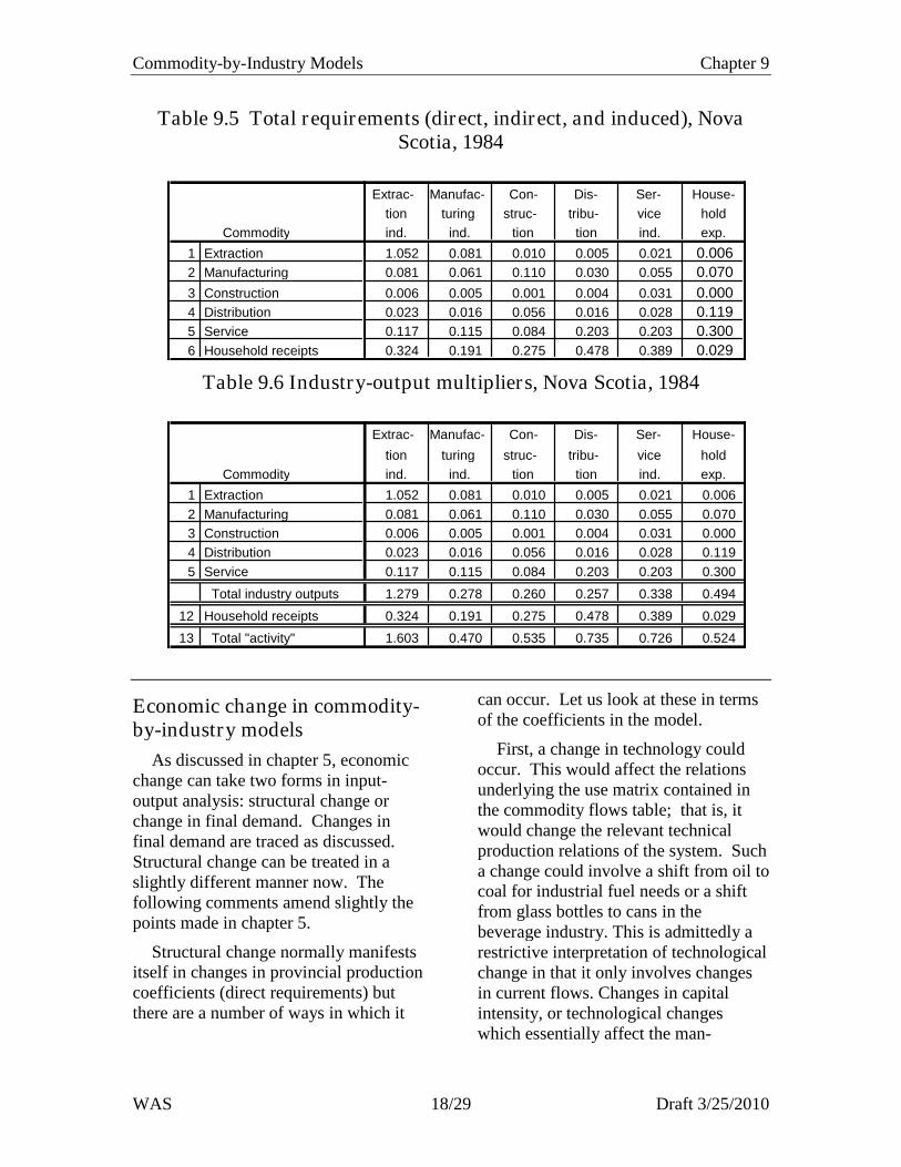
The inverse, (I - A)-1, is called a "total-requirements table" and shows the directand indirect effects of a change in finaldemand. Table 9.5 reports such a tablefor the aggregated system closed withrespect to households . Table 9.6converts these numbers to “multipliers,”properly recognizing the status ofhouseholds as recipient of flows of finalincomes.

Now, we are at the same stage ascompleted in Chapter 5, and can revertto its descriptive elements. Only a fewcomments remain on economic changein the new system.


WAS 18/29 Draft 3/25/2010

Table 9.5 Total requirements (direct, indirect, and induced), NovaScotia, 1984




1 Extraction 1.052 0.081 0.010 0.005 0.021 0.006

2 Manufacturing 0.081 0.061 0.110 0.030 0.055 0.070

3 Construction 0.006 0.005 0.001 0.004 0.031 0.000

4 Distribution 0.023 0.016 0.056 0.016 0.028 0.119

5 Service 0.117 0.115 0.084 0.203 0.203 0.300


Table 9.6 Industry-output multipliers, Nova Scotia, 1984




1 Extraction 1.052 0.081 0.010 0.005 0.021 0.006

2 Manufacturing 0.081 0.061 0.110 0.030 0.055 0.070

3 Construction 0.006 0.005 0.001 0.004 0.031 0.000

4 Distribution 0.023 0.016 0.056 0.016 0.028 0.119

5 Service 0.117 0.115 0.084 0.203 0.203 0.300

Total industry outputs 1.279 0.278 0.260 0.257 0.338 0.494


13 Total "activity" 1.603 0.470 0.535 0.735 0.726 0.524

Economic change in commodity-by-industry models

As discussed in chapter 5, economicchange can take two forms in input-output analysis: structural change orchange in final demand. Changes infinal demand are traced as discussed.Structural change can be treated in aslightly different manner now. Thefollowing comments amend slightly thepoints made in chapter 5.

Structural change normally manifestsitself in changes in provincial productioncoefficients (direct requirements) butthere are a number of ways in which it

can occur. Let us look at these in termsof the coefficients in the model.

First, a change in technology couldoccur. This would affect the relationsunderlying the use matrix contained inthe commodity flows table; that is, itwould change the relevant technicalproduction relations of the system. Sucha change could involve a shift from oil tocoal for industrial fuel needs or a shiftfrom glass bottles to cans in thebeverage industry. This is admittedly arestrictive interpretation of technologicalchange in that it only involves changesin current flows. Changes in capitalintensity, or technological changeswhich essentially affect the man-


WAS 19/29 Draft 3/25/2010

machine relationship, are more difficultto trace through an input-output system.The initial impact of new construction orequipment expenditures may be tracedas a change in final demand. And, if theincrease in output associated with achange in capacity is sold to a final-demand sector, especially as exports, itstotal effect may be traced through thesystem. But many of the effects ofcapital accumulation on economicactivity are transmitted through othermeans. Technological changes in thebroad sense are related to the dynamicquestions of economic growth. Theempirical resolution of these questionsinvolves far more than a static input-output model, and, in fact, far more thanany dynamic economic model incurrent.use.

Second, a change in import patterns,or a change in mij, might occur. The

discovery of domestic oil or the entry ofa major producer of plastic containersmight substantially reduce imports ofthese commodities and thus increase theprovincial flows. A program of importsubstitution might increase provincialflows, delaying the inevitable leakage ofmoney flows from the economy andincreasing the multiplier effect of exportactivity.

Third, alterations in the product mixof local producers may change domesticmarket shares in commodity outputs.These coefficients determine thecommodity content of industry sales inthe provincial interindustry matrix andthus represent one final, probably minor,cause of changes expressed in terms ofthe existing plant structure.

Fourth, new plants in existingindustries may enter the provincialeconomy. A new plant would have theeffect of altering production coefficients

and import patterns in its industry to theextent that its technology and marketareas differ from that of establishedproducers. The significance of thealteration would depend on the size ofthe new plant relative to the rest of theindustry. But only in exceptional casesshould the impact of the structuralchange be more important than theimpact of its sales pattern.

Fifth, a completely new industrymight appear in the province. Thisshould normally be considered part ofthe new-plant alternative discussedabove.

In summary, structural change ininput-output models is primarily a matterof changes in technical productioncoefficients, in domestic market-sharecoefficients, or in import coefficients.


WAS 20/29 Draft 3/25/2010

Illustration 9.1 The simple commodity-by-industry input-output modelfor a region

Symbol definitions:

^ on a vector produces a diagonalmatrix with values from the vector onthe diagonal and zeroes elsewhere.

e is a vector of the sum of domesticfinal demands for commodities.

g is a vector of the values of industryoutputs.

i is a unit (summation) vectorcontaining all ones (Premultiplicationby i sums columns;postmultiplication sums rows).

i as a subscript counts producingindustries.

k as a subscript counts commodities.

j as a subscript counts buying

industries.q is a vector of the values of locally

produced commodity outputs.x is a vector of commodity exports.m is a vector of commodity imports.y is a vector of household incomes

from industriesB is a commodity-by-industry matrix

showing for each industry thecommodity use per dollar of industryoutput. It is the production-coefficients matrix.

D is an industry-by-commodity matrixshowing for each commodity theproportion of the total output of thatcommodity produced in eachindustry. It is the market-sharematrix.

I is the identity matrix (î)U is a commodity-by-industry matrix

showing for each industry the amountof each commodity used.

V is an industry-by-commodity matrixshowing for each commodity theamount produced by each industry.

is a diagonal matrix of commodityimports expressed as proportions oflocal industry and final demands. Itis the import-coefficients matrix.

Definitions or identities:

Industry outputs = Sum of commoditiesproduced

g = Vi (1)Commodity supply = Commodity output+ imports

qs = q + m (2)

Commodity demand = Sum ofintermediate demands, final demandsand exports

qd = Ui + e + x (3)

Behavioral or technical assumptions:

Constant production coefficients

B = Ug -1 or Ui = Bg (4)(elements of commodity-by-industryB are bij = uij/gj, so uij = bijgj )

Constant market-share coefficients

D = Vq -1 or g = Dq (5)(Elements of industry-by-commodity D are dji = vji/qi , so vji

= dijqi .)

Constant import coefficients

= m(Ui + e)-1 or

m = (Bg + e) (6)(Elements of commodity-by-commodity diagonal matrix ofimport coefficients are mk/(jukj +ek). )

Equilibrium condition:

Commodity supply = Commoditydemand

qs = qd, or

q + m = Ui + e + x (7)


WAS 21/29 Draft 3/25/2010

Illustration 9.1 The simple commodity-by-industry input-output modelfor a region (continued)

Solution by substitution:

Problem: given final demands (e' andx'), reduce the number of unknowns toequal the number of equations.

Substitute production (4) and importcoefficients (6) into the equilibriumcondition (7) expressed in terms of q:

q = Bg + e + x - (Bg + e)

Multiply by D to eliminate q andexpress in terms of g (industry outputs)using equation (5):

Dq = D(Bg + e + x - (Bg + e) )

g = D(Bg + e + x - (Bg + e) )

Expand, regroup, and manipulate tosolution in terms of g:

g = DBg + D(e + x) - D(Bg + e) )

g = DBg + De + Dx - D Bg - D e

g = DBg - D Bg +De - D e + Dx

g = D(I - )Bg + D((I - )e + x)

g - D(I - )Bg = D((I - )e + x)

(I - D(I - )B)g = D((I - )e + x)

(I - D(I - )B)-1(I - D(I - )B)g =

(I - D(I - )B)-1D((I - )e + x)

g = (I - D(I - )B)-1D((I - )e + x)

Note in coordination with text:B is total production coefficients, orproportional purchases without regard tolocation of production, expressed incommodity-by-industry terms.

(I - )B is regional productioncoefficients, or proportional purchasesof locally produced outputs, expressedin commodity-by-industry terms.

D(I - )B is regional productioncoefficients expressed in industry-by-industry terms.

(I - D(I - )B)-1 is the inverse, thesolution, or the total requirements

matrix equivalent to that in the simplesolution presented earlier.

D((I - )e + x) is a vector of finaldemands for locally producedcommodities and exports expressed(through premultiplication by D) inindustry terms.

Output multipliers:

gi/xj = rij , where rij is an element of

R=(I - D(I - )B)-1.

Each of these partial outputmultipliers shows the change in localoutput i associated with a change inexports by industry j. Their sum over iis the total output multiplier for industryj.

Income multipliers:

yi/xj = rij*yi/gi), where yi is

household income earned in industry i.

Each of these partial incomemultipliers shows the change inhousehold income in industry i causedby a change in exports by industry j.Their sum over i is the total incomemultiplier for industry j.

Sources:This summary is a variation on the

U.S. model (described in the followingappendix) to include imports and toyield an industry-by-industry model. Italso includes elements of the descriptionof the Canadian system from severalsources such as (Statistics Canada1976). Both sources follow the standardUnited Nations format and symbols.


WAS 22/29 Draft 3/25/2010

Appendix 1 The mathematicsof the United States input-output model

The following mathematics is takenfrom the documentation of the 1987U.S. Interindustry Study. It followsthe standard United Nationscommodity-by-industry systemsymbolically and logically.1

September 1, 1993

MATHEMATICALDERIVATION OF THE TOTAL

REQUIREMENTS TABLES FORTHE INPUT-OUTPUT STUDY 1

The following are definitions:

q is a column vector in which eachentry shows the total amount ofthe output of each commodity.

U is a commodity-by-industrymatrix in which the columnshows for a given industry theamount of each commodity ituses, including Noncomparableimports (I-0 80) and Scrap, usedand secondhand goods (I-0 81).I-0 81 is designated below asscrap.

^ is asymbol that, when placed over avector, indicates a square matrixin which the elements of thevector appear on the maindiagonal and zeros elsewhere.

i is a unit(summation) vector containing

only l's; i is the identity matrix(I).

e is a column vector in which eachentry shows the total finaldemand purchases for eachcommodity from the use table(table 2).

g is a column vector in which eachentry shows the total amount ofeach industry's output, includingits production of scrap.

V is an industry-by-commoditymatrix in which the columnshows for a given commoditythe amount produced in eachindustry. V has columnsshowing only zero entries fornoncomparable imports and forscrap. The estimate of V iscontained in columns 1 - 79 ofthe make table (table 1) pluscolumns of zeros for columns 80and 81.

h is a column vector in which eachentry shows the total amount ofeach industry's production ofscrap. The estimate of h iscontained in column 81 of themake table. Scrap is separated toprevent its use as an input fromgenerating output in theindustries in which it originates.

B is a commodity-by-industrymatrix in which entries in eachcolumn show the amount of acommodity used by an industryper dollar of output of thatindustry. Matrix B is derivedfrom matrix U.

D is an industry-by-commoditymatrix in which entries in eachcolumn show, for a givencommodity (excluding scrap),the proportion of the total output


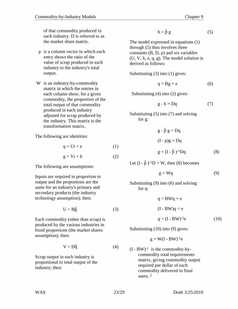
WAS 23/29 Draft 3/25/2010

of that commodity produced ineach industry. D is referred to asthe market share matrix.

p is a column vector in which eachentry shows the ratio of thevalue of scrap produced in eachindustry to the industry's totaloutput.

W is an industry-by-commoditymatrix in which the entries ineach column show, for a givencommodity, the proportion of thetotal output of that commodityproduced in each industryadjusted for scrap produced bythe industry. This matrix is thetransformation matrix.

The following are identities:

q = Ui + e (1)

g = Vi + h (2)

The following are assumptions:

Inputs are required in proportion tooutput and the proportions are thesame for an industry's primary andsecondary products (the industrytechnology assumption); then:

U = Bg (3)

Each commodity (other than scrap) isproduced by the various industries infixed proportions (the market sharesassumption); then:

V = Dq (4)

Scrap output in each industry isproportional to total output of theindustry; then:

h = p g (5)

The model expressed in equations (1)through (5) thus involves threeconstants (B, D, p) and six variables(U, V, h, e, q, g). The model solution isderived as follows:

Substituting (3) into (1) gives:

q = Bg + e (6)


g - h = Dq (7)

Substituting (5) into (7) and solvingfor g:

g - p g = Dq

(I - p)g = Dq

g = (I - p )-1Dq (8)

Let (I - p )-1D = W, then (8) becomes

g = Wq (9)

Substituting (9) into (6) and solvingfor q:

q = BWq + e

(I - BW)q = e

q = (I - BW)-1e (10)


g = W(I - BW)-1e

(I - BW)-1 is the commodity-by-commodity total requirementsmatrix, giving commodity outputrequired per dollar of eachcommodity delivered to finalusers. 2


WAS 24/29 Draft 3/25/2010

W(I - BW)-1 is the industry-by-commodity total requirementsmatrix, giving the industry outputrequired per dollar of eachcommodity delivered to finalusers.2

1 The notation and derivation of thetables presented follow the System ofNational Accounts recommended bythe United Nations. See: A System ofNational Accounts Studies in Methods,Series F No. 2 Rev. 3, United Nations,New York, 1968; also, Stone, R.,Bacharach, M. and Bates, J., "Input-Output Relationships, 1951-1966,"Programme for Growth, Volume 3,London, Chapman and Hall, 1963.

2 Tables are prepared at the detailedand summary levels of aggregation.For the summary tables, theadjustments for secondary productionwere made at the detailed level, thenaggregated before calculation of thetotal requirements tables.

Building Interindustry Models Chapter 10

WAS 25/29 Draft 3/25/2010

10 BUILDING INTERINDUSTRY MODELS

Regional input-output models are,with few exceptions, now produced withcomputer estimating techniquescommonly called "nonsurvey"techniques. This phrase refers to the factthat they are based on the technologyembodied in the national input-output-table and that imports are estimatedbased on some supplementary techniquenot involving extensive survey work.This chapter briefly explains the mostcommon of these approaches.

The basic model

Let us start by restating the basicstructure of the system. The equationsystem for a regional input-output modelmay be written as

aijq jj1

n

+ yiff 1

t

+ ei = xi (i=1...n) (10-1)

The aij represent purchases from

regional industry i by industry j (or xij)

as a proportion of the output of industry j(or xj), yif is the local final demand for

the products of industry i by final-demand sector f, and ei is the exports by

industry i. The equation system mightbe illustrated with an algebraic tablesimilar to that in Figure 5.1.

The system can also be outlined interms of supply, describing theproduction technology of a region:

n

ijijqa

1

+ vfjf1

t

+

n

ijijqm

1

=qj

(j=1...n) (10-2)

Here vfj is the value added by final-

payments sector f to the product ofindustry i, and mij is the imports of the

products of industry i by industryexpressed as a proportion of the output

of industry j. (Note that we haveincluded t local final-payment sectors tomatch the t local final-demand sectors.This is for simplicity, since we normallyhave more final-demand sectors thanfinal-payment sectors.

Now assume that we have augmentedthe interindustry portion of the systemby treating the household sector as anindustry, as in Chapter 5. The aijmatrix, written as A, is called theregional interindustry coefficients matrixand is a critical part of the system sinceits constancy is a major technicalassumption in input-output analysis. Asis clear from Chapter 5, the solution tothe equation system 10-1 may be writtenin matrix form as

(I - A)-1*(Y + E) = X (10-3)

We will use this form of the system toavoid repetitive algebra in the discussionof estimating techniques.

The regional coefficients matrix, A,may be regarded as the differencebetween a technology matrix, P, and animports matrix, M:

A = P - M (10-4)

The technology matrix recordspurchases from industry i (regardless oflocation) by industry j as a proportion ofthe output of industry j (pij). The imports

matrix contains the mij elements in

equation 10-2. The major problemconfronting the regional analyst inconstructing a transactions table isobtaining the P matrix and dividing itinto its component parts, A and M. Wenow turn to this division problem.


WAS 26/29 Draft 3/25/2010

Estimating techniques

Given the system described above, theregional analyst has several proceduresavailable to him in constructing hisempirical model. The choice betweenthese techniques depends largely uponthe resources available. This sectionbriefly outlines these procedures anddescribes the means by which aninexpensive nonsurvey procedure maybe evolved into a survey-basedtechnique to fit whatever budget isavailable.(Schaffer 1972; Schaffer andChu 1969)

Survey-only techniques

Properly, an input-output model isbased on a full survey of industries andfinal consumers which documents bothsales and purchases. Each respondent isasked to designate sales to regionalindustries (xij) and to final users inside

(yif) and outside (ei) the region. The

respondents are also asked to designatetheir purchases from regional industries(aijqj), their purchases from industries

outside the region (mijxj), and their final

payments (vfj ) to primary resource

owners in the form of wages andsalaries, profits, depreciation allowances,taxes, etc. These purchases and finalpayments outline the productiontechnology of each industry in a usableformat, already separated into a regionalflows matrix and an imports matrix.

In acquiring data on both purchasesand sales, the analyst has assembled theinformation required to produce apotentially reliable table. But the table isalso very expensive and its constructionis very time consuming. Notice whathappens if you don’t have a completecensus of firms and perfect reporting ineach case. In this perfect case, the rowestimates of xij will be identical to the

column estimates. Now notice whathappens if you have sampled only a fewfirms: the row estimates and the columnestimates now vary widely. Samplingproblems and reporting errors aresubstantial and the analyst is forced toachieve balance by tediously assayingthe reliability of responses and byjuggling numbers until totals finallymatch.

A basic alternative to this full-surveyapproach is the “rows-only” method.First used by Hansen and Tiebout, thismethod assumes

... that firms know the destination of theiroutputs far better than the origin of theirinputs, especially where regional breakdownsare required. In other words, in terms of input-output flows, information for the "rows" iseasier to obtain than information for the"columns.” The reason for this is that thebundle of inputs is usually so varied andcomplex that their origins are difficult even forfirms involved to track down accurately.However, the same firms are especiallyconcerned with where and to whom they selltheir output. (Hansen and Tiebout 1963)

This approach permits the analyst toavoid a complex data reconciliation. Itproduces only one entry per cell in thetransactions table; the full-surveymethod forces the analyst to check hiswork by producing two estimates of cellvalues.

A second alternative to the full-surveyapproach is what is called the “columns-only” method. This approach assumesthat business firms know their sources ofsupply better than they do the locationsof their customers. Harmston and Lundargue that this approach takes advantageof the detailed knowledge ofexpenditures required by businessmenfor control and tax purposes (Harmstonand Lund 1967). Producing data in thesame simple form as that of the rows-only method, the columns-only approach


WAS 27/29 Draft 3/25/2010

seems well-suited for use in smallregions characterized by a relativelylarge number of locally-owned firms.

The supply-demand pool procedure

A nonsurvey technique commonlyused in the United States, the supply-demand pool technique relies on thenational input-output table as areasonable estimate of the production-technology matrix, or P matrix, of aregion and proceeds to estimate regionalflows and imports using the concept ofregional commodity balances (Isard1953). This method is sometimes calledthe Moore-Petersen technique since itwas first applied to a study of Utah byMoore and Petersen (Moore andPetersen 1955).

The only additional data assumed tobe available are gross outputs for the nregional industries, qj, and the grosspurchases of t final-demand sectors.Now, to avoid more complex addition,let us assume that the P matrix includesboth industries and final-demand sectors,so A is of dimension n*(n+1). Valueadded is three rows in the national tableand has been excluded from P.

Let di be the row sum of totaldemands for the products of industry i,computed from A as follows:

di =j=1

n+t

pijxj (10-5)

Here, of course, the pij have been

computed from the national input-outputtable and we have simply reducednational flows to regional size.

A commodity-balance ratiocomparing regional production or supply(qi) with regional demand can be

computed as

bi = qi/di (10-6)

and the P matrix can be divided into itsA and M components through a simpleset of rules. If bi is greater than or equal

to one, then all inputs can be supplied bylocal producers and we can set aij = pij,

mij = 0, and ei = qi - di. If bi is less than

one, inputs must be imported, soaij=bipij, mij = pij-aij and ei=0.

This pool procedure allocates localproduction, when adequate, to meet localneeds; when the local output isinadequate, it allocates to eachpurchasing industry i a share of regionaloutput qi based on the needs of the

purchasing industry itself (pijqj) relative

to total needs for output i (di).

Export-survey method

One of the major characteristics of aregional input-output model is itsopenness. Exports and imports aresubstantial, if not dominant, parts of thetypical regional transactions table. Sincesimulated exports are so greatly atvariance with the survey-based exportsin the above comparison, it seemsreasonable to believe that correction ofthis discrepancy could lead to a muchbetter estimate of regional transactions.

If we can afford neither of the morepowerful alternatives to a full survey asdiscussed above, then an export surveycombined with a supply-demand poolprocedure may be an adequate substitute.This approach requires that we simplycanvass firms in the region, asking forthree bits of information: their industryclassification, value of sales for the year,and the proportion of their sales going toout-of-region purchasers. The first twoanswers permit the analyst to classifyreplies and to properly weight export


WAS 28/29 Draft 3/25/2010

proportions in constructing thetransactions table.

The procedure, then, involves settingexports of each industry i at the survey-estimated value and simulating theremainder of the table. For the balanceratio used above, we simply substitute aratio which excludes exports from thesupply available for local use:

bei =

qi - ei

di

(10-7)

This approach satisfies exportrequirements first and then allocates theremainder of local production tosatisfying local needs in proportion to

requirements. If bei is greater than one,

the technology matrix may have to beadjusted, but this proves to be a minorproblem.

Selected-values method

Now, if more trade information thanjust export estimates can be assembled,the method can be extended to permit asetting of selected values in thetransactions table. We simply setobserved values xig, xih, ..., xik and

estimate the remaining regional flowsusing an adjusted balance ratio:

bsi =

qi ei x ig xih ... x

ik

di xig x ih ... xik

(10-8)

Known-trade method

The development of the commodity-origins table in the new commodity-by-industry format suggested a slightvariation on this system. What if weknow some imports as well as someexports? This makes the formula into

bki =

qi mi ei

di

(10-9)

Here the numerator contains supplyavailable for local use (local supply isequal to local demand less imports andlocal supply less exports is the amountavailable for local use) while thedenominator is simply local demands.This method would be used if a localsurvey provided technical coefficientsand estimates of imports and exports, aswas the case in our Nova Scotia study(DPA Group Inc. and Schaffer 1989).

This method is tricky when bothimports and exports are "known" for thesame commodity. The supply-demandequation has to balance, and this surelymeans that one of the known values hasto be adjusted. Tricky, but that'sstatistics.

.

table of contents, chapters 8-10rri.wvu.edu/webbook/schaffer/chapters 8-10 s10 combyindmod.pdf ·...

Documents