systems failure and safety assessment using integrated
TRANSCRIPT

1
Systems Failure and Safety Assessment Using Integrated Petri Net Modeling andFault Tree Analysis Approaches
Angela Adamyan and David He*
Department of Mechanical and Industrial EngineeringThe University of Illinois at Chicago
Chicago, Illinois 60607
Abstract
Current methods in combining Petri net modeling with fault tree analysis for systems
failure and safety assessment assume that the failure rates of the basic events in a system
are the same and the Petri net model of the system consists of only simple structures.
These assumptions do not reflect the real industrial applications for system failure and
safety analysis. To overcome the limitations of the current methods for systems failure
and safety assessment, this paper extends the current methods to real applications where
basic events can have different failure rates and the systems can be modeled with
complex Petri net structures. Examples of failure and safety analysis of a nuclear waste
carrying manipulator and an automated manufacturing and assembly system with a robot
are provided to demonstrate the developed method.
Key words: Petri nets, fault tree analysis, system reliability and safety, failure rates.
* To whom correspondence should be addressed

2
1. Introduction
The reliability and safety analysis of complex systems and processes is becoming a moreand more difficult task due to the rapid technology evolution and increasing complexityof the systems that, in turn, often causes the increase of failure rate of the systems. Afailure is defined as an event when a required function is terminated, or exceedsacceptable limits (IEC 50(191)). For reliability and safety assurance, failures of thesystems have to be traced and analyzed.
A variety of methods for failure analysis exist, for example, reliability block diagram(RBD), failure mode and effect analysis (FMEA), and fault tree analysis (FTA). Amongthe methods, FTA is a widely accepted and used technique for analysis of system failures.However, FTA has several drawbacks; for example it represents only logic relations.Petri net is an alternative to FTA since it is graphically symbolizes the cause and effectrelationships among the events. In addition, it represents and analyses dynamic behaviorof the system, which greatly helps in tracing the failures and allows performingcomprehensive failure and reliability analysis of the system. Several authorsdemonstrated the superiority of Petri nets over FTA (Yang and Liu, 1997; Lin and Chiou,1997).
The limitation of the fault trees urged researchers to combine FTA with other techniquesto achieve enhanced results for failure analysis. To overcome the limitations of fault treeanalysis technique in system failure analysis, Petri nets have been combined with faulttree analysis to determine the failure rate of the systems. Yang and Liu (1997)investigated the dynamic behavior of Petri nets with failure rates formulation. However,their method has several limitations. First, it implies that the times between failures ofdifferent components are same. Second, the method does not take into the account thepossibility of loops and inhibitor arcs in Petri net modeling. Those limitations do notallow representing real-life systems completely. Therefore, to perform a comprehensivefailure and safety analysis of complex systems, we extended the method to the systemswith loops, inhibitor arcs and with basic events that have different failure rates.
The remainder of the paper is organized as following. In Section 2, we provide abackground of fault tree analysis, the general idea of Petri net modeling and conversionmethods of fault trees to Petri nets. In Section 3, the methodology of combining Petrinets with fault tree analysis is extended to include a real application scenario where basicevents have different failure rates and the system is modeled with complex Petri netstructures. In Section 4, examples of failure and safety analysis of a nuclear wastecarrying manipulator and of an automated manufacturing and assembly system with arobot are provided to demonstrate the developed method. Finally, Section 5 concludesthe paper.

3
2. Background
In this section, a brief description of fault tree analysis, Petri net modeling, and acorrelation between them is provided.
2.1. Fault tree analysis
A fault tree arises from the logic diagram that is used to analyze the probabilitiesassociated with various causes and their effects. FTA starts by identifying a problem(catastrophic accident or other undesirable result) and all possible ways that the problem(or failure) occurs. FTA has been widely used for obtaining reliability information aboutcomplex systems since 1960. The importance of FTA was pointed out in a safety study ofthe US Nuclear Regulatory Commission (1975). In addition, FTA is a powerful designtool that can help to meet product performance objectives.
Minimal cut set is a set of components, in which the repair of any failed component willresult in functioning of the failed system. FTA is equivalent to the minimal cut set treewith all minimal cut set in an AND-structure. A minimal cut-AND structure is a set, inwhich the failed state of the output becomes true when all states of the inputs existsimultaneously. Therefore, it is very important to estimate the output of the minimal cut-AND-structure in order to quantify the top event of the fault tree.
2.2. Petri nets
Petri nets are widely used as a tool for analyzing system safety and reliability of thecomplex systems. They can be used as visual communication aid similar to flow charts,block diagrams, fault trees and networks. The use of Petri nets augments the ability ofunderstanding the interaction between various effects. First developed by Adam Petri inthe early 1960’s, Petri nets have become a powerful and generic tool for modeling andsimulation (Peterson, 1981; Holliday and Vernon, 1987; Murata, 1989; Ramaswamy andValavanis, 1994; Liu and Chiou, 1997). The Petri nets where random delays areexponentially distributed are referred to as stochastic timed Petri nets (SPNs) (Zhou,1995; Molloy, 1982, 1985; Florin et al., 1991). General-purpose software packages areavailable for solving SPN models, including GreatSPN (Chiola, 1987) and SPNP (Ciardo,1989).
Al-Jaar and Desrochers (1990) have demonstrated that Petri net modeling is superior overtraditional Markov chain modeling in that the number of places and transitions increasesslightly as the system complexity increases, whereas the number of states in the Markovchain increases exponentially. In addition, Petri net modeling provides a general andformal procedure to generate all possible states for analysis.
Formally, Petri net is a directed bipartite graph defined by a 6-tuple( ) ( )[ ],,,,,, 0 tOtIMAPTN = where { }ntttT ,,, 21 �= is a set of transitions, each transition
representing an event or an action; and { }lpppP ,,, 21 �= is a set of places, where aplace is used to represent either the condition for the event or the consequences of the
4
event. Therefore, before building a Petri net model, the events and their conditions andconsequences in a system are first defined, and then are represented by transitions andplaces in a Petri net. Each place can contain one or more tokens. Movement of tokensthrough the places in the constructed model simulates the process of the system thatallows identifying and analyzing what can go wrong within the system. A place with (orwithout) a token indicates that the state represented by the place is true (or false).
{ } { }TPPTA ×∪×⊆ is a set of directed arcs that connect transitions to places and placesto transitions. 0M is the initial marking of the system that represents initial state of thesystem. A marking M, can also be represented as a vector { }lmmmM ,,, 21 �= , where mi
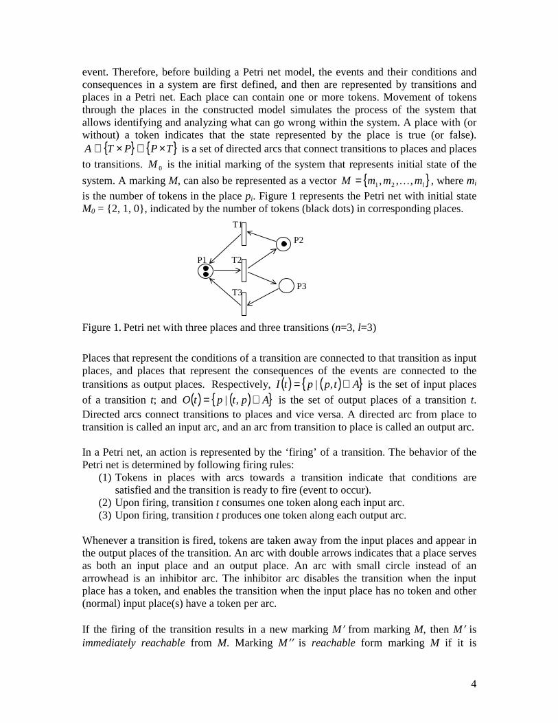
is the number of tokens in the place pi. Figure 1 represents the Petri net with initial stateM0 = {2, 1, 0}, indicated by the number of tokens (black dots) in corresponding places.
Figure 1. Petri net with three places and three transitions (n=3, l=3)
Places that represent the conditions of a transition are connected to that transition as inputplaces, and places that represent the consequences of the events are connected to thetransitions as output places. Respectively, ( ) ( ){ }AtpptI ∈= ,| is the set of input placesof a transition t; and ( ) ( ){ }AptptO ∈= ,| is the set of output places of a transition t.Directed arcs connect transitions to places and vice versa. A directed arc from place totransition is called an input arc, and an arc from transition to place is called an output arc.
In a Petri net, an action is represented by the ‘firing’ of a transition. The behavior of thePetri net is determined by following firing rules:
(1) Tokens in places with arcs towards a transition indicate that conditions aresatisfied and the transition is ready to fire (event to occur).
(2) Upon firing, transition t consumes one token along each input arc.(3) Upon firing, transition t produces one token along each output arc.
Whenever a transition is fired, tokens are taken away from the input places and appear inthe output places of the transition. An arc with double arrows indicates that a place servesas both an input place and an output place. An arc with small circle instead of anarrowhead is an inhibitor arc. The inhibitor arc disables the transition when the inputplace has a token, and enables the transition when the input place has no token and other(normal) input place(s) have a token per arc.
If the firing of the transition results in a new marking M′ from marking M, then M′ isimmediately reachable from M. Marking M′′ is reachable form marking M if it is
T1
P1
P2
P3
T2
T3

5
reachable form any marking that is immediately reachable from M. The reachability treeis a graphical representation of all markings of a net starting from its initial marking. Inother words, the reachability tree is the state diagraph in which each node represents theunique marking, i.e. state of the system, and edges represent the possible state transitions.
2.3. Transformation of fault trees to the Petri nets
The Petri net graphical representation can be used to construct the cause and effectrelationship among the events. Since boolean logic symbols are commonly used toaccount for failure causation, to convert fault trees to Petri net one needs to examine logicgates based on Petri nets representation. According to enabling rules every logic gate canbe represented by a Petri net model. Liu and Chiou (1997) have demonstrated that Petrinets in failure analysis can be used to replace logic gate functions in a fault tree. Thetransition of the fault trees to the Petri net representations allows performing thoroughfailure and reliability analysis of the systems, as well as provides efficient way forobtaining path sets and minimal cut sets. Some examples of the correlation between faulttrees and Petri nets are shown in Figure 2. For more detailed explanation of thetransformation of fault trees to Petri nets readers can refer to (Yang and Liu, 1997).
Figure 2. Correlation between a fault tree and a Petri net
3. Determining failure rates of systems using petri nets
The first step, in determining the failure rates of the system, is identifying the basicfailures with help of the fault here analysis. Once the failures of the system are identifiedthey incorporated to the Petri net representation. One can analyze the dynamic behaviorof a system and determine its failure rate by computing the timed markings of places inthe Petri net representing the system. Yang and Liu (1997) demonstrated this
OR-modelAND-model
P3
P1 P2
P3
P1 P2P1 P2
P3 P3
P1 P2
R out of PNmodel
R
P1 PN
…
R
P2 PNP1
…
Inhibit gatemodel
P1
P2
P3P3
P1 P2

6
methodology with an airbag inflator system failure analysis. In this section, themethodology presented by Yang and Liu (1997) is extended to complex Petri netstructures and real application cases where basic failure events have different failurerates. The derivations of formulations to compute the timed markings of the places in aPetri net are presented next.
Define:
mi(t) - the marking of the place PiTi - time between failures of basic event idi - delay time of the transition imi(t)dj - represents the marking of place i followed by the transition j in the direction of
the top eventk - the state of the system
mi(t) indicates the token quantity at time t for place i. The number of markings of theplace Pi appeared after time t performs like a stair function. It is equal to zero during thefirst period, one during the second period, two during the third period, etc. Therefore, thetime marking for a place can be written as:
( ) ( ) ( )[ ] ( ) ( )[ ]( ) ( )[ ] ( ) ( ) ( ) ( )�
∞
=
−=+−+−+−=+−−−+
+−−−+−−=
1
32322
210
kkTtuTtuTtuTtuTtuTtu
TtuTtuTtututm
��
where u(t) is a unit step function.
The timed marking transfer of places can be divided in to the following categories: (1)Transition with single input (single and hierarchical input transitions); (2) Transition withmultiple inputs (OR- and AND-model with single and hierarchical level of transitions);(3) Transition with single input and loop; (4) Transition with inhibitor arcs. Thederivation of the marking of a top event output place in each category is explained next.
3.1. Transition with single input
In this category, the marking for an output place is the input marking with time delay dinvolved. Two cases are discussed in this category: (1) single transition and (2) multipletransitions.
Case 1: Single transition
Figure 3 reveals the output place with single transition and single input place.
Figure 3. Single transition with single input placem1
m2
d
(1)

7
According to (1), the marking of the input place m1 can be written as:
( ) ( )�∞
=
−=1
1k
kTtutm
Hence,
( ) ( )�∞
=
−−=1
2k
dkTtutm
Case 2: Hierarchical structure
Figure 4 reveals a hierarchical structure where each place has only single input transitionand single input place.
Figure 4. Hierarchical structure
The output marking is computed based on the first input place (2) and delay time of eachtransition in the structure.
( ) ( ) ( ) ( )��∞
=
−−=−−−−−==1
21,,1 ,21k
topdddtop DkTtudddkTtutmtmtop
��
where �
=
=top
ssdD
1 and denotes the total delay time.
3.2. Transition with multiple inputs
In this category, depending on the types of transitions involved, two subcategories aredistinguished: OR-and AND-structures.
(2)
(3)
m1
m2
d1
d2
...
mtop
dtop
(4)

8
3.2.1 OR-structures
According to the property of Petri nets the output marking of an OR-structure is thesummation of input markings with delay times, i.e.,
( ) ( ) ( ) ( )[ ]ndnddtop tmtmtmtm +++= �
21 21
In this subcategory, depending on the level of the transitions involved, two cases arediscussed: (1) single level transition and (2) multiple level transitions.
Case 1: Single level transition
Figure 5 reveals OR-structure, i.e. single transition has multiple input places
Figure 5. Single level transition with multiple-inputs for the OR-structure
From (1), the markings of the basic places can be computed as:
( ) ( )�∞
=−=
111
kkTtutm
( ) ( )�∞
=−=
122
kkTtutm
( ) ( )�∞
=−=
1knn kTtutm
Substituting (6) into (5) will produce the top place marking as:
( ) ( ) ( ) ( )
( )� �
���
=
∞
=
∞
=
∞
=
∞
=
��
���
� −−=
=−−++−−+−−=
n
s kss
knn
kktop
dkTtu
dkTtudkTtudkTtutm
1 1
1122
111 �
(5)
...
(6)
(7)
m2 mnm1
d1 d2 . . .
mtop
dn

9
Case 2: Multiple level transitions in OR-structure
Figure 6 reveals OR-structure with multiple level transitions.
Figure 6. Multiple level transitions with multiple-inputs in OR-structure
From (5) and in accordance with Figure 6 we can write:
( ) ( ) ( )[ ] ( ){ } ( ) ( )
( ) ( {[ [ ( ) ( ) ] ( ) }
( ) ) ( ) ] ( ) =−−+−−++−−+
+−−+−−+−−=+
+��
���
�++�
�
�
� +++=
���
���
∞
=−−
∞
=−
∞
=
∞
=
∞
=
∞
=−
−
−
−
−
−
111
123
166
144
122
1111
36421
27
531
2
37
65
4321
ktoptopd
ktopd
k
dk
dkk
dtop
ddtop
dddddddtop
dkTtudkTtudkTtu
dkTtudkTtudkTtutm
tmtmtmtmtmtm
top
top
top
top
�
�
��
( )
( )+−−−−−−+
+−−−−−−=
�
�
∞
=−
∞
=−
125322
125311
ktop
ktop
ddddkTtu
ddddkTtu
�
�
m5
. ..
m2
d1 d2
m1
m4
d3 d4
m3
mtop-1
dtop-2 dtop-1
mtop-2
mtop

10
( )
( )
( ) ( )
( ) [ ( ) ]
( )�
���� �
��
�
�
∞
=−−
−
=+
∞
=
−
=
∞
= =−
∞
=−−
∞
=−−−
∞
=−
∞
=−
−−+
+−−−+−−=
=−−+−−−++
+−−−−−−+
+−−−−−−+
111
1
12221
1
11 1121
111
1233
129766
127544
ktoptop
R
suuss
k
R
sk
R
ss
ktoptop
ktoptoptop
ktop
ktop
dkTtu
ddkTtudkTtu
dkTtuddkTtu
ddddkTtu
ddddkTtu
�
�
�
�
where R=[(top-2)+1]/2
3.2.2 AND-structure
In an AND–structure a transition is fired only when there are tokens available in allfeeding places. Therefore, the output marking of an AND-structure is equal to thesmallest marking among input markings, i.e.,
( ) ( ) ( ) ( )[ ]dnddtop tmtmtmtm ,,,min 21 �=
Similar to the OR-structure, based on the level of the transitions involved, two cases ofthe AND-structure are discussed: (1) single level transition and (2) multiple leveltransitions.
Case 1: Single transition with multiple-input places in an AND-structure
Figure 7 reveals the AND-structure with single transition.
Figure 7. Single level transition with multiple-inputs in AND-structure
From (6) and (9), the top place marking of Figure 7 can be computed as:
( ) [ ( ) ( ) ( ) ]
( ) ( )nidkTtu
dkTtudkTtudkTtutm
kb
kn
kktop
�
�
3,2,1 ,
,,,min
1
112
11
=−−=
=−−−−−−=
�
���
∞
=
∞
=
∞
=
∞
=
(8)
(9)
m2. . .
mtop
mnm1
d
(10)

11
where Tb is the largest number among Ti, i=1, 2, …,n. In other words, the tokengeneration period of Pb is the longest among all the input places.
Case 2: Multiple transitions with multiple-inputs in an AND-structure
Figure 8 reveals the case of an AND-structure with multiple level transitions.
Figure 8. Multiple level transitions with multiple-inputs for the AND-structure
From (9) and Figure 6, the top place marking is computed as:
( ) ( [ { [ ( { [ ( ) ( ) ] } ( ) ) ]( ) } ] ( ) ) =
=
− rr dtopddd
dddddtop
tmtm
tmtmtmtm
16
4211
,
,,,minminmin
43
3221
�
�
[ ( )
( )
( )
( )
( )
( ) ] =−−
−−−−−
−−−−−
−−−−
−−−−
−−−−−=
�
�
�
�
�
�
∞
=−
∞
=
∞
=
∞
=
∞
=
∞
=
11
1548
1436
1324
1212
1211
,,
,
,
,
,min
kRtop
kR
kR
kR
kR
kR
dkTtu
dddkTtu
dddkTtu
dddkTtu
dddkTtu
dddkTtu
��
�
�
�
�
. ..
m2
d1
d2
m1
m4m3
mtop-1
dR
mtop-2
mtop
m5

12
[ ( )
( )
( ) ] ( )RdkTtu
dkTtu
dkTtu
k
R
ss
k
R
ss
k
R
ss
�,4,3,2 ,
,
,min
1 22
1 12
1 11
=−−
−−
−−=
� �
� �
� �
∞
= =
∞
= =
∞
= =
νν
ν
3.3 Transition with single input and loop
In Figure 9, single transitions with single inputs in a loop are presented.
Figure 9. Transitions with single inputs in a loop
According to (4) marking mn-1 is computed as:
( ) ( ) ( )�∞
=− −−==
−1
,,11 1,21k
dddn DkTtutmtmn�
, where �−
=
=1
1
n
ssdD .
In the case of Petri net loop-structure, any marking of the loop can be computed as:
( ) ( ) ( ) ( )( ) ( )�∞
=− −−=+++=
1121 ,
kns lDkTtutmtmtmltm � ,
where TD
tldDn
ss +
==�=
,1
3.4. Transition with an inhibitor arc
A Petri net with an inhibitor arc is presented in Figure 10.
(11)
m1
m2
d1
d2
...
dn
mn-1
(13)
(12)

13
Figure 10. Transition with an inhibitor arc
When m2 > 0, the inhibitor arc disables the transition d1, when m2 = 0 and m1 > 0transition d1 is enabled. The marking m3(t) can be written as
( ) ( )�∞
=
+−−=1
213k
ddkTtutm
Based on formulas (1) to (14) any top event marking can be derived.
4. Illustrative examples
In this section, two examples are provided to demonstrate the application of thedeveloped method. The first example is the failure analysis of a nuclear waste carryingmanipulator and the second example is the safety analysis of an automated manufacturingand assembly system with a robot.
4.1 Failure analysis of a nuclear waste carrying manipulator
Failure of a nuclear waste carrying manipulator can be very catastrophic, causing deathsand injuries. The fault tree analysis for detecting possible failures of a nuclear wastecarrying manipulator has been presented in Zhao, et al. (2000).
The nuclear waste carrying manipulator is used to carry and pack drums in a nuclearwaste storehouse. The drums are filled with low radiation wastewater mixed with cement.The failure of carrying manipulator is characterized by the falling and collision of drums.Falling and collision of drums could cause cracking and deforming that is not permeated.The fault three for the collision of drums is presented in Figure 12.
When the caring manipulator works in the storehouse, cracking and deforming of drumscaused by falling and collision are not permitted. The main cause of a drum falling is notonly of the failure of mechanical but also the transverse collision. In the following parts,transverse collision of drums acts as top event and FTA technology is applied (see Figure11). The remaining of the symbols in the fault tree is as shown on the Appendix A.
(14)
m1
m3d1
d3
mn
m2
m4
d2
d4

14
Figure 11. The fault tree of collision of drums containing solidified nuclear waste (Zhao,et al., 2000)
In this paper, the original fault tree presented in Zhao, et al. (2000) is transformed intoPetri net to illustrate the proposed failure analysis method.
The organization of control system is shown in Figure 12.
T
E1 E2
E3 E4C13E13C14 C15
E5 E6 E7 A1 A2 E14 E3
E9 E10
B3
C2 E16 E15
E12
C11 C12C10 E8 B1
C1
A3 B4 E17 E7
E18 B6
C3 C4 C5 C6 B5 E19
C4 C7 C9 B2 C16 C17 C19C18
1
1
2
2

15
IPC
Operation param
eter display
Operation m
ode setter
Operation state display
Manual control equipm
ent
D.C
. driver
D.C
. motor
Gearing
Photo encoder
Limit sw
itching and photo switches
photo encoder
brake
Figure 12. Control system structure (Zhao, et al., 2000)
Next step to apply technology is transferring the fault tree to the Petri net. In Figure 13,the corresponding Petri net structure for the fault tree in Figure 11 is presented. Thedescription of places for the Petri net in Figure 13 is presented in Appendix B, and thedescription of delays is presented in Appendix C.
X4
CPU
communication input output
CPU
fast counter input output
Pulpit-PLC Bridge-PLC
control panel

16
Figure 13. The Petri net of collision of drums containing solidified nuclear waste
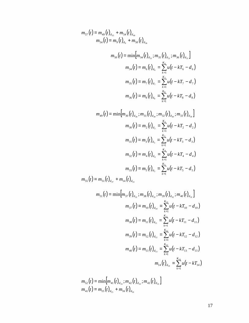
Based on (2) to (11) the marking transfer for of collision of drums containing solidifiednuclear waste as shown in Figure 13 can be derived as follows:
( ) ( ) ( )[ ]4545 636164 ;min dd tmtmtm =
( ) ( ) ( ) ( )38431 5259161 ddd tmtmtmtm ++=
( ) ( ) ( )[ ]4141 555759 ;min dd tmtmtm =
d38
d30
d31
d32d36
d35 d40 d40 d42
d27
d26
d19 d44 d29
d14 d18d17d15 d16
d21d20 d9
d13d10 d11 d12
d39
d25d22 d23 d24
d5 d2 d3 d4
d6 d7 d8
d33d41
d45
d43 d1
P61
P64
P63
P57 P55 P41 P42
P1 P59 P52 P19 P62 P29
P43
P15 P16P51 P14P49
P54 P44 P60
P39 P40P37 P38
P50 P9
P36P34 P35
P32 P33P30 P31
P20 P21 P28P58
P27P56
P53 P26
P47 P48P45 P46
P4 P5 P2 P3
P24 P25P22 P23
P17 P18
P12 P13P10 P11
P7 P8 P6d34
d28
17
( ) ( ) ( )4035 544957 dd tmtmtm +=
( ) ( ) ( )369 50954 dd tmtmtm +=
( ) ( ) ( ) ( )[ ]313131 36353450 ;;min ddd tmtmtmtm =
( ) ( ) ( )�=
−−==6
61
66634
K
kd dkTtutmtm
( ) ( ) ( )�=
−−==7
71
77735
K
kd dkTtutmtm
( ) ( ) ( )�=
−−==8
81
88836
K
kd dkTtutmtm
( ) ( ) ( ) ( ) ( )[ ]30303030 3332313049 ;;;min dddd tmtmtmtmtm =
( ) ( ) ( )�=
−−==2
21
22230
K
kd dkTtutmtm
( ) ( ) ( )�=
−−==3
31
33331
K
kd dkTtutmtm
( ) ( ) ( )�=
−−==4
41
44432
K
kd dkTtutmtm
( ) ( ) ( )�=
−−==5
51
55533
K
kd dkTtutmtm
( ) ( ) ( )1437 145155 dd tmtmtm +=
( ) ( ) ( ) ( ) ( )[ ]32323232 4039383751 ;;;min dddd tmtmtmtmtm =
( ) ( ) ( )�=
−−==10
101
10101037
K
kd dkTtutmtm
( ) ( ) ( )�=
−−==11
111
11111138
K
kd dkTtutmtm
( ) ( ) ( )�=
−−==12
121
12121239
K
kd dkTtutmtm
( ) ( ) ( )�=
−−==13
131
13131340
K
kd dkTtutmtm
( ) ( )�=
−=14
141
1414
K
kd kTtutm
( ) ( ) ( ) ( )[ ]333333 43424152 ;;min ddd tmtmtmtm =
( ) ( ) ( )1615 161541 dd tmtmtm +=

18
( ) ( )�=
−=15
151
1515
K
kd kTtutm
( ) ( )�=
−=16
161
1616
K
kd kTtutm
( ) ( ) ( )�=
−−==17
171
17171742
K
kd dkTtutmtm
( ) ( ) ( )�=
−−==18
181
18181843
K
kd dkTtutmtm
( ) ( )�=
−=1
11
11
K
kd kTtutm
( ) ( ) ( ) ( )294419 29621963 ddd tmtmtmtm ++=
( ) ( ) ( )[ ]4242 604462 ;min dd tmtmtm =
( ) ( ) ( )2120 212044 dd tmtmtm +=
( ) ( )�=
−=20
201
2020
K
kd kTtutm
( ) ( )�=
−=21
211
2121
K
kd kTtutm
( ) ( ) ( )[ ]2828 585760 ;min dd tmtmtm =
( ) ( )445728 dtmtm =
( ) ( ) ( )[ ]2727 275658 ;min dd tmtmtm =
( ) ( ) ( )2642 265356 dd tmtmtm +=
( ) ( ) ( ) ( ) ( )[ ]34343434 4847464553 ;;;min dddd tmtmtmtmtm =
( ) ( ) ( )�=
−−==22
221
22222245
K
kd dkTtutmtm
( ) ( ) ( )�=
−−==23
231
23232346
K
kd dkTtutmtm
( ) ( ) ( )�=
−−==24
241
24242447
K
kd dkTtutmtm
( ) ( ) ( )�=
−−==25
251
25252548
K
kd dkTtutmtm
( ) ( )�=
−=26
261
2626
K
kd kTtutm

19
( ) ( )�=
−=27
271
2727
K
kd kTtutm
( ) ( )�=
−=29
291
2929
K
kd kTtutm
( ) ( )�=
−=19
191
1919
K
kd kTtutm
The failure rate of this system can be written as:
( ) ( )t
tmtF 64= .
4.2 Safety analysis of an automated manufacturing and assembly system with robot
Development of automated manufacturing systems requires diverse new skills and setsnew challenges for operators. It also increases the possibility of errors due to theorganization of the processes and the human factor. In this section, the safety analysis ofan automated manufacturing and assembly system with robot is used to illustrate theapplication of the developed method. The system makes one product type and needs onemachining operation and one assembly operation. Figure 14 presents the systemconsisting of one assembly station (A), one robot (R), and one machine (M). Thefollowing steps describe the production procedure:
Figure 14. An automated manufacturing and assembly system with robot
(1) M starts to operate(2) After M finishes its operations R takes and transfers the part from M to A(3) R begins the assembly
At the first step of modeling, an abstract Petri net of the system is constructed andrevealed in Figure 15 that states that the production procedure needs a machine operationfollowed by unloading the part, and an assembly operation. Robot transfers parts from themachine to the assembly station and starts assembling the product.
AssemblyStation
A
MachineM
Robot R

20
Figure 15. Petri net model of the robotic manufacturing cell
The automated operation of the robot continues even when the robot drops the part. Thepart must be recovered by the operator, therefore the operator has to enter hazardous zonewhere she/he can be struck by the robot. Robot applications with absolute safety cannotbe achieved; therefore accidents of this type happen. At the second step of modeling, anabstract Petri net of the system is specified as described in Figure 16, which states thatthe operator is entering the hazardous zone once the part is dropped. The failures ofinterlock or power source lead to the accident where the operator is struck by the robot.
Figure 16. Petri net model of the robotic manufacturing cell with failure
m8
T6
m1
d5
m10
d7
m7
d4
m6
m2
m1
d1
m5
d2
m3m4
d3
Machiningoperation
Power sourceis not cut off
Partavailable
Part onassemblystation (A)
Aavailable
Aoperation
UnloadMachine
Robot RavailablePart droppedand operator isready to enterhazardous zone
Failure ofpower sourceOperator is
entering
Operator isstruck bymanipulator
Systemstopped
Operator isin danger
Interlock isready to fail
Power sourceis ready to fail
mP
Machineavailable
m2
m1
d1
m5
d2
m3m4
d3
Machiningoperation
Partavailable
Part onassemblystation (A1)
Aavailable
Aoperation
UnloadMachine
Robot Ravailable
Machineavailable

21
Based on (2) to (11) the marking transfer for the machining and assembly system withfailure as shown in Figure 16 can be derived as follows:
( ) ( ) ( )77 10711 dd tmtmtm +=
( ) ( ) ( )[ ]65 9810 ,min dd tmtmtm =
( ) ( )�∞
=
−−=1
588 5k
d dkTtutm
( ) ( )�∞
=
−−=1
699 6k
d dkTtutm
( ) ( ) ( ) ( ) ( )2224 25467 dddd tmtmtmtmtm ++==
( ) ( )112 dtmtm =
( ) ( )�∞
=
−−=1
111 2k
d dkTtutm ,
To determine the markings for m4 and m5 we have to take into the account the fact thattransition d3 has an inhibitor arc, therefore:
( ) ( ) )()(72 11354 dd tmtmtmtm −==
( ) ( ) ( ) ( )222 5423 ddd tmtmtmtm ++=
Note that markings m4 and m5 are safe markings, i.e., they can get values of 1 and 0. Thevalue of those markings is equal to 1 during time delay d2 and 0 during time delay d3.
Therefore, m4 and m5 =1 if decimal part of 32
1
32 ddd
ddt
+≤
+ ,
m4 and m5 =0, otherwise.
The failure rate of this system can be written as:
( ) ( )t
tmtF 11= .
5. Conclusions
The assessment of failure and safety of complex systems and processes plays animportant role in improving the usability of systems and hence decreasing the hazardousimpacts on the environment. To overcome the limitations of fault tree analysis technique

22
in system failure and safety analysis, Petri nets have been combined with fault treeanalysis to determine the failure rate of the systems.
The current methods in combining Petri net with fault tree analysis for systems failureand safety assessment assume that the failure rates of the basic events in the systems arethe same and consider only Petri nets where more complex structures such as loops andinhibitor arcs cannot be used. In most of the cases, Petri nets with loops and inhibitorarcs often model the real life systems. To overcome the limitations of the currentmethods for systems failure and safety assessment, this paper extended the currentmethods to real applications where basic events can have different failure rates and thesystems can be modeled with complex Petri net structures. Two examples are providedto demonstrate the developed method.
The method can be used as a comprehensive risk assessment process that providesmanagers with a tool for analyzing hazardous operations for improving safety of theworkers and environment, as well as the overall safety of the processes. Data can also beused for helping the industry to meet safety requirements and to improve the efficiency ofnew manufacturing system implementations. The results obtained can contribute to thesafety, environmental, and ergonomic aspects in designing and operating systems.

23
APPENDIX: The Meaning of the Symbols in the Fault Tree and the Description ofPlaces and Delays in the Petri Net for the Failure Analysis of the Nuclear WasteCarrying Manipulator
A. The Meaning of the Symbols in the Fault Tree (Figure 11)T Transverse collision of drums containing nuclear waste happens.E1 Transverse collision happens between obstacle and the drum in the gripper, which is
caused by bridge moving when the gripper is not at upmost position.E2 Transverse collision happens between the drum in the gripper and the drum on forth
layer, which is caused by bridge moving when the gripper is at upmost position.E3 Operator fails to stop the machine on time.E4 The bridge moves when the gripper is not at upmost positionE5 The switchgears break down.E6 Measuring failsE7 Control failsE8 Measuring components failE9 D.C. Drivers fail to stopE10 Power in pulpit is not cut off when D.C. Drivers failsE12 Control and executive components in pulpit failE13 Bridge over runsE14 Bridge fails to stop moving automatically in timeE15 Setting failsE16 Position of gripper is over moved to set positionE17 Measuring failsE18 Position error is caused by measuring components failureE19 Measuring components failA1 The operators neglect their dutyA2 The right person has not been chosen for the jobA3 The setting operations is wrongB1 Measuring component failure has not been detected by programB2 The controlling program has errorB3 The controlling program has errorB4 Supervision computer fails to recognize the setting errorB5 Measuring component failure has not been detected by programB6 The measuring program has errorC1 Circuit breakers cannot be switched offC2 Emergency circuit cannot be switched offC3 Limit-switch fails to switch offC4 The CPU of PLC1 failsC5 The input module of PLC1 failsC6 The memory of PLC1 failsC7 The D.C. Drivers failsC9 The output module of PLC1 failsC10 The CPU of PLC2 failsC11 The switchgears failC12 The output module of PLC2 fails

24
C13 There are obstacles in the routC14 There is drum in the gripperC15 There are drums on the 4th layer in the moving directionC16 The high speed counting modules failC17 Photo switches lose pulsesC18 Photo encoder loses pulsesC19 Encoder slips off gear
B. The Description of Pleases in the Petri Net Model (Figure 13)P1 There are obstacles in the routP2 The CPU of PLC1 ready to failP3 The D.C. Drivers failsP4 The controlling program has errorP5 The output module of PLC1 ready to failP6 The CPU of PC2 failsP7 The switchgears failP8 The output module PLC2 ready to failP9 The controlling program has errorP10 Limit-switch ready to fail to switch offP11 The CPU of PLC1 ready to failP12 The input module of PLC1 ready to failP13 The memory of PLC1 ready to failP14 Measuring component failure has not been detected by programP15 Circuit breakers cannot be switched offP16 Emergency circuit cannot be switched offP17 The operators are not availableP18 Person selection errorP19 There is drum in the gripperP20 The setting operations is wrongP21 Supervision computer fails to recognize the setting errorP22 The high speed counting modules ready to failP23 Photo switches pulses are not availableP24 Photo encoder pulses are not availableP25 Encoder is not stableP26 Measuring component failure has not been detected by programP27 The measuring program has errorP28 Control failsP29 There are drums on the 4th layer in the moving directionP30 The CPU of PLC1 failsP31 The D.C. Drivers ready to failP32 The controlling program does not function properlyP33 The output module of PLC1 failsP34 The CPU of PC2 ready to failP35 The switchgears ready to failP36 The output module PLC2 failsP37 Limit-switch fails to switch off

25
P38 The CPU of PLC1 failsP39 The input module of PLC1 failsP40 The memory of PLC1 failsP41 The switchgears break downP42 The operators neglect their dutyP43 The right person has not been chosen for the jobP44 Setting failsP45 The high speed counting modules failP46 Photo switches lose pulsesP47 Photo encoder loses pulsesP48 Encoder slips off gearP49 D.C. Driver fails to stopP50 Control and executive components in pulpit failP51 Measuring components failP52 Operator fails to stop the machine in the time.P53 Measuring components failP54 Power in pulpit is not cut off when D.C. Drivers failsP55 Measuring failsP56 Position error is caused by measuring components failureP57 Control failsP58 Measuring failsP59 The bridge moves when the gripper is not upmost positionP60 Position of gripper is over moved to set positionP61 Transverse collision happens between obstacle and the drum in the gripper, which is
caused by bridge moving when the gripper is not at upmost position.P62 Bridge fails to stop moving automatically in time and over runsP63 Transverse collision happens between the drum in the gripper and the drum on forth
layer, which is caused by bridge moving when the gripper is at upmost position.P64 Transverse collision of drums containing nuclear waste happens.
C. List of Delays in the Petri Net Model (Figure 13)d1 Rout is contaminatingd2 The mean time to failure of the CPU of PLC1d3 The mean time to failure of the D.C. Driversd4 The controlling program error progressing timed5 The mean time to failure of the output module of PLC1d6 The mean time to failure of the CPU of PLC2 failsd7 The mean time to failure of the switchgearsd8 The mean time to failure of the output module PLC2d9 The controlling program error proceeding timed10 The mean time to failure of the limit-switch to switch offd11 The mean time to failure of the CPU of PLC1d12 The mean time to failure of the input module of PLC1d13 The mean time to failure of the memory of PLC1d14 Measuring component failure has not been detected by programd15 The mean time to failure of the circuit breakers, it cannot be switched off

26
d16 The mean time to failure of the emergency circuit, it cannot be switched offd17 Time the operators are not availabled18 Operator selection timed19 The mean time to have a drum in the gripperd20 Operations settingd21 Supervision computer failure rate to recognize the setting errord22 The high speed counting modules mean time to failured23 Photo switches pulses mean time to failured24 Photo encoder pulses mean time to failured25 Encoder is not stabled26 Measuring component failure time to detect errord27 The measuring program processing timed28 The mean time to failure of the controld29 The mean time to have drum on the 4th layer in the moving directiond30 The mean time to failure of CPU of PLC1 and PLC2, D.C. Drivers, controlling
program, and output module of PLC1d31 The mean time to failure of CPU of PLC2, switchgears, and output module PLC2d32 The mean time of failure of output module PLC2, limit-switch, the CPU of PLC1,
and input module of PLC1d33 The mean time to failure of switchgears break, operators duty, and correct person
selectiond34 The mean time to failure of high speed counting modules, photo switches, photo
encoder, and encoder slips off geard35 The mean time to failure of D.C. Driver to stopd36 The mean time to failure of control and executive components in pulpitd37 The mean time to failure of measuring componentsd38 The mean time to failure of operator to stop the machine on timed39 The mean time to failure of measuring componentsd40 The mean time to failure of power in pulpit when D.C. Drivers failsd41 The mean time to failure of control and operator to stop the machine on timed42 The mean time to failure of settings and position of gripperd43 The mean time to failure of the bridge moving when the gripper is not at upmost
positiond44 The mean time to failure of transverse collision that happens between obstacle
and the drum in the gripper, which is caused by bridge moving when the gripperis not at upmost position.
d45 The mean time to failure of bridge to stop moving automatically in time and overruns and transverse collision of drums containing nuclear waste

27
References
Al-Jaar, R., Y., and Desrochers, A. A., 1990, “Performance Evaluation of AutomatedManufacturing Systems Using Generalized Stochastic Petri Nets”, IEEE Transactionson Robotics and Automation, Vol. 6, No. 6, pp. 621 – 639.
Chiola, G., 1987, “A Graphic Petri Net Tool for Performance Analysis”, Proceedings ofInternational Workshop on Modeling Techniques and Performance Evaluation,France, pp. 323 – 333.
Ciardo, G., 1989, Manual for the SPNP Package, Duke University.
Florin, G., Fraize, C., and Natkin, S., 1991, “Stochastic Petri Nets: Properties,Applications, and Tools”, Microelectronics Reliability, Vol. 31, No. 4, pp. 669 – 697.
Holliday, M. A., and Vernon, M. K., 1987, “A Generalized Timed Petri Net Model forPerformance Analysis”, IEEE Transactions on Software Engineering, Vol. SE – 13,No. 12, pp. 1297 – 1310.
IEC 50(191), 1990, International Electrotechnical Vocabulary (IEV), Chapter 191-Dependability and quality of service, International Electrotechnical Commission,Geneva.
Liu, T. S. and Chiou, B. S, 1997, “Application of Petri nets to failure analysis”,Reliability Engineering and System Safety, Vol. 57, pp. 129-142.
Long, W., Sato, Y., and Horigone, M., 2000a, “Quantification of Sequential FailureLogic for Fault Tree Analysis”, Reliability Engineering and System Safety, Vol. 67,pp 269-274.
Molloy, M. K., 1982, “Performance Analysis Using Stochastic Petri Nets”, IEEETransactions on Computers, Vol. 3, No. 9, pp. 913 – 917.
Molloy, M. K., 1985, “Discrete Time Stochastic Petri Nets”, IEEE Transactions onSoftware Engineering, Vol. SE-11, No. 4, pp. 417 – 423.
Murata, T., 1989, "Petri Nets: Properties, Analysis, and Applications", Proceedings ofthe IEEE, Vol. 77, No. 4, pp. 541 - 579.
Peterson, J. L., 1981, Petri Net Theory and the Modeling of Systems, Prentice Hall,Englewood Cliffs, NJ.
Ramaswamy and Valavanis, 1994, “Extended Petri Net-Based Modeling, Analysis AndSimulation Of An Intelligent Materials Handling System”, Journal of Intelligent andRobotic Systems: Theory & Applications, Vol. 10, No1, pp. 79-108.

28
US Nuclear Regulatory Commission, 1975, “An Assessment of Accident Risk in U.S.Commercial Nuclear Power Plants”, Reactor Safety Study WASH-1400 (NUREG-75/014), Washington, DC.
Yang, S. and Liu, T, 1997, “Failure Analysis for an Airbag Inflator by Petri Nets, ”Quality and reliability Engineering International, Vol., 13, pp. 139-151.
Zhao, D., Cai, L., Gao, C., and Sun, Yukun, 2000, “Application of FTA in OperationSafety Design of Nuclear Waste Carrying manipulator” Proceedings of the 3rd WorldCongress on intelligent Control and Automation, Hefei, China, pp. 729-732.
Zhou, M. and Venkatesh, K., 1998, Modeling, Simulation, and Control of FlexibleManufacturing Systems: A Petri Net Approach, World Scientific, Singapore.
Zhou, M. and Zurawski, R., 1995, “Introduction to Petri Nets in Flexible and AgileAutomation,” in Petri Nets in Flexible and Agile Automation, Zhou (Ed), Kluwer,Norwell, MA, pp. 1 – 42.