rail service failure prediction:an integrated approach
TRANSCRIPT

‘-
1
Rail Service Failure Prediction: An Integrated Approach Using Fatigue Modeling and Data Analytics
Faeze Ghofrani, Seyedsina Yousefianmoghadam, Qing He, Andreas Stavridis
TAIM 2019
State College, PAOctober 2019

‘-
2
CONTENTS1. Introduction
2. Research Overview
3. Background
4. Methodology
5. Case Study
6. Results
7. Conclusions

‘-
3
Maintenance
Descriptive
Optim
ization
Image
Processing
SVM
AN
N
…….
Ghofrani et al. (2018)
Introduction: BDA in RTS
The application of big data analytics in railway transportation systems

‘-
4
Research OverviewA Comprehensive study on the Application of
BDA in RTS
PredictiveDescriptive Prescriptive
MaintenanceSafety Operations
PreventiveCorrective Condition-Based
TrackVehicle Signaling Equipment

‘-
5
The relationship between Geometry Defects and Rail
Defect Occurrence
Rail Defects Service Failures
Predicting Frequency (rate) of
Rail Defects
Predicting the Risk of Reoccurrence of
Rail Defects
Service Failure Occurrence in
Heavy Haul Rail Lines
Predicting Frequency (rate) of
Service Failures
Track
Geometry Defects
Binary Classification
An Ensemble Physics-informed Data driven
Simulation
Survival Analysis Binary Classification
An Ensemble Physics-informed Data driven
Simulation
Research Overview-Continued
‘-
6
Rail Service Failure Prediction: An Integrated Approach Using Fatigue Modeling and Data Analytics

‘-
7
• Develop a data-driven growth prediction model to forecast how an existing defect grows to a complete failure in future?
• Assess the potential (rate) of service failures• Approach: Fatigue Modeling, combined with Data Analysis
Research Objective
Ongoing in this studyGhofrani et al. (2019)

‘-
8
Data-driven Model
Mechanics Model
Service Failures in Literature
Ensemble Model
Machine Learning Models
Empirical Equations Developed Using Experimental Data

‘-
9
Methodology Framework
Determining the MGT thresholds required for a crack of specific size to
propagate to a service failure
Assuming prior distributions for size
and frequency of cracks
Simulation based on Approximate Bayesian Computation (ABC)
framework
Calculating the posterior distribution for size and
frequency of cracks
Predicting frequency of service failures
Mechanics Modeling with FEM
Data Analytics with ABC
Carried out mainly by structural engineering group
Carried out mainly by transportation engineering group at UB

‘-
10
Methodology: Finite Element Modeling of the Rail
Detail fracture (TDD) is mainly concentrated inside the rail
A rail element was created in ABAQUS
UIC60 (60E1) rail profile geometry was used
Elastic steel material was used (E=200 Gpa)

‘-
11
Methodology: Finite Element Modeling of the Rail Hexahedra structured mesh was used for the rail
A defect was modeled inside the rail head
width varied from 15 mm to 55 mm with increments of 10
mm
depth kept equal to 10 mm
inclined with respect to the longitudinal direction of the rail
(12.5 degrees) (Zhou et al. 2017)
XFEM-crack method was used to overlay defects to the original
mesh

‘-
12
Methodology: Finite Element Modeling the Rail Stress induced to the section containing the defect is affected by the location of
the wheel
Moment and shear demand profiles were obtained for the considered section:
Defected section
‘-
13
Methodology: Finite Element Modeling the Track
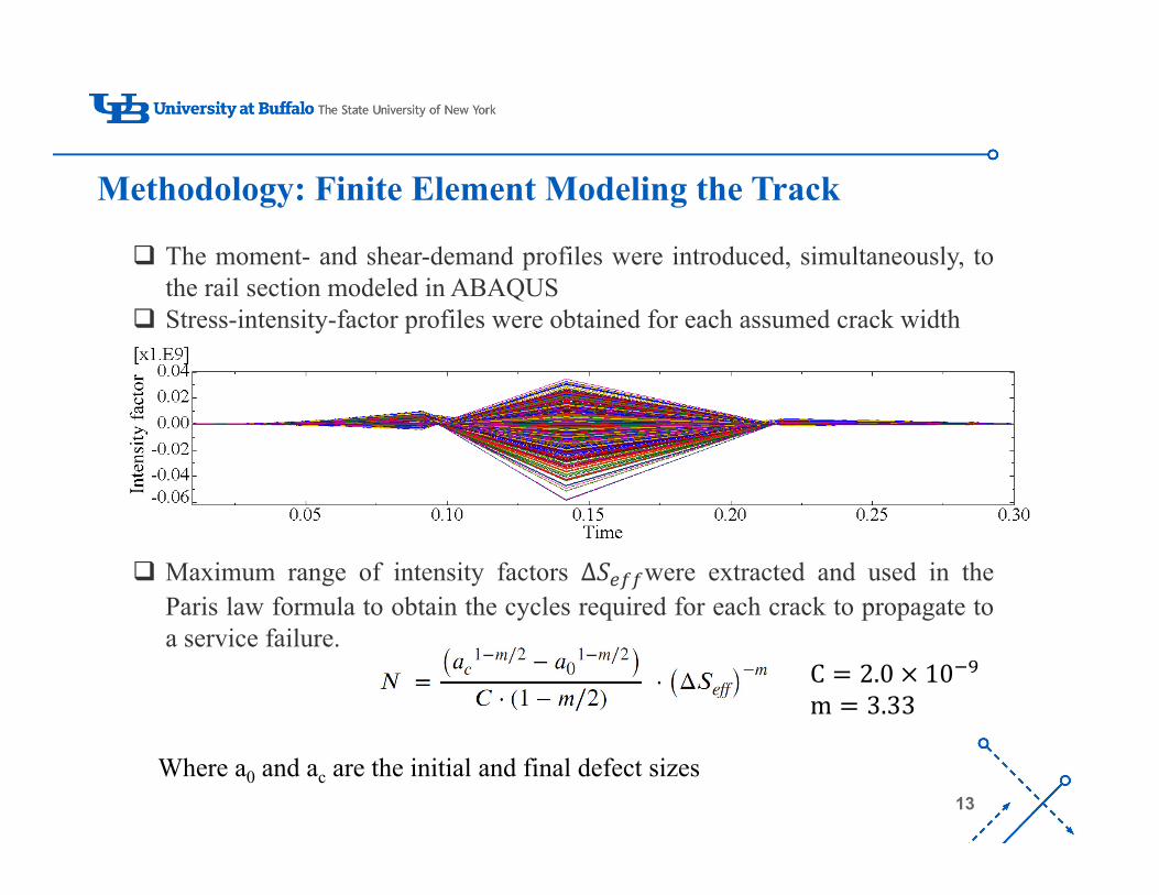
The moment- and shear-demand profiles were introduced, simultaneously, tothe rail section modeled in ABAQUS
Stress-intensity-factor profiles were obtained for each assumed crack width
Maximum range of intensity factors ∆𝑆 were extracted and used in theParis law formula to obtain the cycles required for each crack to propagate toa service failure.
C 2.0 10m 3.33
are the initial and final defect sizescand a0Where a

‘-
14
Methodology: Finite Element Modeling the Track
Number of cycles for crack growth is converted to equivalent accumulatedtraffic load (MGT), by multiplying it by the load from each wheel (Frýba,1996)
Intensity factor (M𝑃𝑎 𝑚 . )
Initial crack size (m)
Final size (m) N MGT
34.5 0.015 0.073 60098 10.2235.5 0.025 0.073 30465 5.1843.3 0.035 0.073 9522 1.6245.2 0.045 0.073 4945 0.8444.0 0.055 0.073 2936 0.5
0.073

‘-
15
Methodology: ABC Rejection Algorithm
Bayes’ Theorem in General
ABC Rejection algorithm
Start with a sample of parameter points from prior distribution 𝑝 𝜃 . Each sample parameter point θ is simulated using an evolution model and
simulated data Ď is generated. If the generated dataset Ď varies significantly from the observed dataset D, then
the parameter point θ is rejected.p(D, Ď) ε
The outcome of this process is a posterior distribution of parameter points withouthaving to calculate the likelihood
𝑝 𝜃|𝐷𝑝 𝐷|𝜃 𝑝 𝜃
𝑝 𝐷
Posterior Evidence
PriorLikelihood

‘-
16
Case Study: Data Preparation
Track Tonnage Defects and Service Failures
Inspections and Grinding
Selecting Segments
Removing Segments Overlaps
Dividing Segments
Assigning a Unique ID for each Segment
Assigning Defects and service
failures to Track Segments
Allocating attributes of
segments using ID
Input Dataset
Processing
Output Dataset An integrated Dataset with Required Variables for Modeling Purpose
Temperature
Data provided by FRA from a Class I US Railroad from 2011 to 2016
National Oceanic and Atmospheric Administration (NOAA)

‘-
17
Case Study: Data Description
Defect Type Percentage of total
Ordinary Break 28.38
Transverse Detail Fracture 20.36
Thermite Weld 14.11
Bolt Hole Break 4.90
Crushed Head 4.26
Most frequent defect types that are causing service failures
Service failure dispersion over the studied US Class I network
Number of Service Failures vs Average Temperature
Data has been provided by CSX for six years 2011-2016

‘-
18
Case Study: Integration of Mechanistic And Statistical Model
The function gets segment information as input
It draws number of cracks for each segment (λp) from a
Poisson distribution
It draws size of each crack from a discrete uniform
distribution
It checks if the drawn cracks would turn into a service failure
(using segment MGT and FEfunction)
It calculates number of defects that turn into service failures
The function returns simulated number of service
failures for each segment
Functions
Function FE- Input: Crack/Defect Size, Output: Required MGT to Complete Breakage (FEM Output)
Function G- Input: Segment Information, Output: Simulated Number of Service Failures

‘-
19
λ1 λ2 λ3
n_serv 1
Prior distribution of the model parameter, number of crack (λ): assumed as discrete uniform distribution
n_defects
Observational data
1. Summary statistic (n_serv) from observational data computed
2. n simulations are performed by drawing parameter values from the prior distribution for each segment
3. The summary statistic (𝑛_𝑆𝑒𝑟𝑣) is computed for each simulation using Function G
4. Based on the distance and a tolerance, we decide for a simulation whether its summary statistics to be kept or to be rejected (𝐷𝑖𝑠𝑡𝑎𝑛𝑐𝑒 𝑛_𝑠𝑒𝑟𝑣 , 𝑛_𝑆𝑒𝑟𝑣 𝜀))
5. The posterior distribution of λ is approximated using thedistribution of parameter values λi of accepted simulations
Posterior distribution of model parameter λ
Simulation 1 Simulation 2 Simulation 3 Simulation n
n_serv 2 n_serv 3n_serv n
Case Study: Integration of Mechanistic And Statistical Model Functions- ContinuedFunction Posterior- ABC Rejection Algorithm

‘-
20
Partition the dataset into train and test sets
For the segments in train set, the posterior
distribution of λ is calculated (using
POSTERIOR Function)
Fitting a log-linear regression model on train
data segments, the coefficients of each
variable is determined
The computed variable coefficients are used to predict λ for test dataset
Simulated number of failures are computed
using Function G
The average difference between simulated service failures and
observed failures of all segments are calculated
as the error metric
Case Study: Integration of Mechanistic And Statistical Model Main Algorithm
MGT, Weight, Age, Geometry and Rail Defects, Inspection, Grinding, Temperature, Curvature, Grade
‘-
21
Results and Discussions
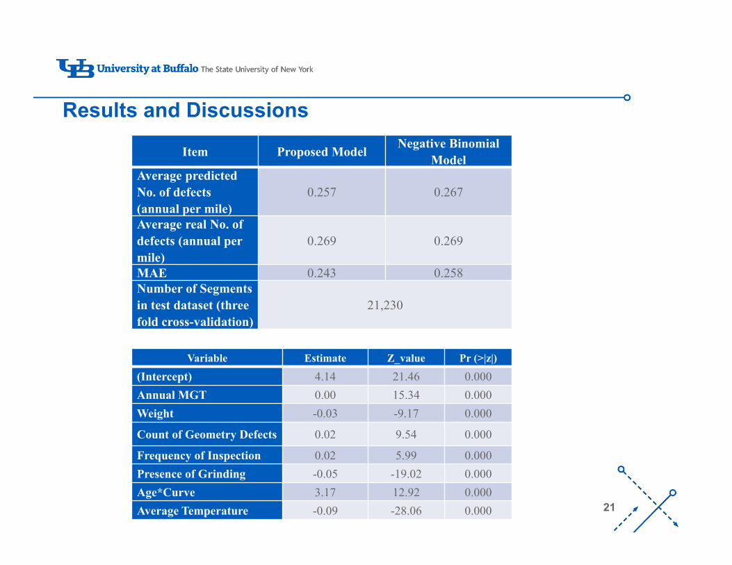
Item Proposed Model Negative Binomial Model
Average predicted No. of defects (annual per mile)
0.257 0.267
Average real No. of defects (annual per mile)
0.269 0.269
MAE 0.243 0.258Number of Segments in test dataset (three fold cross-validation)
21,230
Variable Estimate Z_value Pr (>|z|)
(Intercept) 4.14 21.46 0.000Annual MGT 0.00 15.34 0.000Weight -0.03 -9.17 0.000
Count of Geometry Defects 0.02 9.54 0.000
Frequency of Inspection 0.02 5.99 0.000Presence of Grinding -0.05 -19.02 0.000Age*Curve 3.17 12.92 0.000Average Temperature -0.09 -28.06 0.000

‘-
22
Contributions of the Study
Designing a comprehensive logical methodology framework for datacollection, pre-processing, and modeling based on a collection of datasetsfrom different resources in a Class I railroad
We develop a hybrid physics-informed statistical model for calculating therate of service failures
The developed method is applied to the prediction of service failurefrequency obtained from the inspections in a Class I Railroad.
The results of the proposed method is validated by comparing to the resultsof other popular count-data models in the literature
‘-
23
Conclusions
Incorporating the physics-based behavior of the railway track on a
segment is accompanied with a better estimation of the probable
occurrence of service failures.
Regarding railroad applications, service failure frequency is part of their
scoring system to calculate the rail quality and determine the rail renewal
for the next year.
It can help on identifying the black spots in the rail track network to
prioritize their corrections.
Therefore, the outcome of this paper can be used to guide how to make
decisions of capital planning for railroads.

‘-
24
Acknowledgement
The data was provided by CSX. Authors would like to express their sincerethanks for the support from CSX.

‘-
25
References
Schafer, D H, & Barkan, C. P. L. (2008). A hybrid logistic regression/neural network model for the prediction of broken rails. In Proceedings of the 8th World Congress on Railway Research, Seoul, Korea.
Schafer, Darwin H., & Barkan, C. P. L. (2008). A Prediction Model for Broken Rails and an Analysis of thier Economic Impact. Proceedings of the American Railway Engineering and Maintenance-of-Way Association Annual Conference, 252(847).
Liu, X., Lovett, A., Dick, T., Rapik Saat, M., Barkan, C. P., 2014. Optimization of ultrasonic rail-defect inspection for improving railway transportation safety and efficiency. Journal of Transportation Engineering 140 (10), 04014048.
Ghofrani, F., He, Q., Mohammadi, R., Pathak, A., & Aref, A. (2019b). Bayesian Survival Approach to Analyzing the Risk of Recurrent Rail Defects. Transportation Research Record: Journal of the Transportation Research Board, 2673(3), 281–293.

‘-
27
Function G (p) # given the data related to segment p, simulate the number of service failures
define cracks as a list of size Tdefine n_serv as a list of size T initialized with 0 For t in 1 to T do
if t>1 for crack in cracks[t-1] do
if t*MGTp > FE(crack) n_serv[t] = n_serv[t] + 1 remove crack from cracks[t-1]
endend
endn_cracks ~ Poisson (𝜆p) For i in 1 to n_cracks do
cracks[t][i] ~ DiscreteUniform(15, 75) if MGTp > FE(cracks[t][i]) or cracks[t][i] >= 55
n_serv[t] = n_serv + 1 end
endend
end

‘-
28
function POSTERIOR (n_serv, MGT)λ = [] distances = [] for m in 1 to M do
λm~ uniform[0, 10]λ = λ + λmn_defect = G(λm, MGT) distance = DITANCE (n_serv, n_serv) distances = distances + distance
enduse ABC framework to reject distances higher than a threshold
and find λposteriorReturn λposterior
end

‘-
29
For fold=1 to K dotrain_data, test_data = PARTITION(data, fold, K) 𝜆 = [] MGT = [] W = []S = [] For p in train_data do
𝜆 = POSTERIOR(n_servp, MGTp)𝜆 𝜆 𝜆
MGT = MGT + MGTpWeight = Weight + WeightpSpeedp = Speed + SpeedpGeo_Def p = Geo_Def + Geo_Def pInspection p = Inspection + Inspection p
Grinding p = Grinding + Grinding pTemperature p = Temperature + Temperature p
end# fit log-linear regression on train data log(𝜆 ) = β+ α1*MGT + α2*Speed +α3*Weight+ α4* Geo_Def + α5* Inspection + α6* Grinding + α7* Temperature
# use the regression coefficients to predict 𝜆 for test datan_defects = []
𝑛_𝑑𝑒𝑓𝑒𝑐𝑡𝑠 = []For p in test_data do
lambda_p = exp(β+ α1*MGT + α2*Speed + α3*Weight+ α4* Geo_Def + α5* Inspection + α6* Grinding+α7*Temperature)
𝑛_𝑠𝑒𝑟𝑣 ℎ𝑎𝑡 = G(𝜆 , MGTp)n_serv = n_serv + n_servp
𝑛_𝑠𝑒𝑟𝑣 ℎ𝑎𝑡 = 𝑛_𝑠𝑒𝑟𝑣 ℎ𝑎𝑡 + 𝑛_𝑠𝑒𝑟𝑣 ℎ𝑎𝑡print(metric(n_serv, 𝑛 ℎ𝑎𝑡 ))
endEnd