Tectonophysics 532–535 (2012) 61–81

Contents lists available at SciVerse ScienceDirect

Tectonophysics

j ourna l homepage: www.e lsev ie r .com/ locate / tecto

Review Article

Systematic comparisons of earthquake source models determined using InSAR andseismic data

Jennifer Weston a,⁎, Ana M.G. Ferreira a,b, Gareth J. Funning c

a School of Environmental Sciences, University of East Anglia, Norwich, UKb ICIST, Instituto Superior Técnico, Technical University of Lisbon, Lisbon, Portugalc Department of Earth Sciences, University of California, Riverside, USA

⁎ Corresponding author.E-mail address: J.weston@uea.ac.uk (J. Weston).

0040-1951/$ – see front matter © 2012 Elsevier B.V. Alldoi:10.1016/j.tecto.2012.02.001

a b s t r a c t

a r t i c l e i n f o

Article history:Received 31 May 2011Received in revised form 30 January 2012Accepted 2 February 2012Available online 21 February 2012

Keywords:InSARSeismologyEarthquake source parametersJoint inversionsSpatial geodesy

Robust earthquake source parameters (e.g., location, seismic moment, fault geometry) are essential for reli-able seismic hazard assessment and the investigation of large-scale tectonics. They are routinely estimatedusing a variety of data and techniques, such as seismic data and, more recently, Interferometric SyntheticAperture Radar (InSAR). Comparisons between these two datasets are frequently made although not usuallyin a comprehensive way. This review compares source parameters from global and regional seismic cata-logues with those from a recent database of InSAR parameters, which has been expanded with 18 additionalsource models for this study.We show that moment magnitude (Mw) estimates agree well between the two datasets, with a trend forthrust events modelled using InSAR to have slightly larger Mw estimates. Earthquake locations determinedusing InSAR agree well with those reported in regional catalogues, with a median difference of 6.3 km be-tween them, which is smaller than for global seismic catalogues. We also investigate the consistency ofsource parameters and source directivity by comparing ISC hypocentres with GCMT and ICMT centroid loca-tions for earthquakes with Mw≥6.5. In some cases the source directivity is qualitatively comparable withprevious studies, especially when comparing ISC and ICMT locations. The average difference betweenInSAR-determined depths and those in the EHB catalogue is reduced if a layered half-space is used in the in-version of InSAR data. Overall, faulting geometry (strike, dip and rake angles) remain in good agreement withvalues from the GCMT catalogue, and any large discrepancies can be attributed to tradeoffs between param-eters. With continued investment in satellites for radar interferometry, InSAR is a valuable technique for theestimation of earthquake source parameters. The observed trends and discrepancies between InSAR and seis-mically determined source parameters are the result of issues with the data, different inversion techniquesand the assumed Earth structure model.

© 2012 Elsevier B.V. All rights reserved.

Contents

1. Introduction . . . . . . . . . . . . . . . . . . . . . . . . . . . . . . . . . . . . . . . . . . . . . . . . . . . . . . . . . . . . . . . 622. Investigating earthquakes using InSAR data . . . . . . . . . . . . . . . . . . . . . . . . . . . . . . . . . . . . . . . . . . . . . . . . 62

2.1. Principles and progress of the technique . . . . . . . . . . . . . . . . . . . . . . . . . . . . . . . . . . . . . . . . . . . . . . 622.2. Modelling surface deformation using InSAR . . . . . . . . . . . . . . . . . . . . . . . . . . . . . . . . . . . . . . . . . . . . . 63

3. Seismological modelling of earthquakes . . . . . . . . . . . . . . . . . . . . . . . . . . . . . . . . . . . . . . . . . . . . . . . . . . 643.1. Inversion methods and source catalogues . . . . . . . . . . . . . . . . . . . . . . . . . . . . . . . . . . . . . . . . . . . . . . 64

4. Earthquake source parameter comparisons . . . . . . . . . . . . . . . . . . . . . . . . . . . . . . . . . . . . . . . . . . . . . . . . 654.1. Moment and moment-magnitude . . . . . . . . . . . . . . . . . . . . . . . . . . . . . . . . . . . . . . . . . . . . . . . . . 654.2. Earthquake location and source directivity . . . . . . . . . . . . . . . . . . . . . . . . . . . . . . . . . . . . . . . . . . . . . 67

4.2.1. Source directivity . . . . . . . . . . . . . . . . . . . . . . . . . . . . . . . . . . . . . . . . . . . . . . . . . . . . . 704.3. Depth . . . . . . . . . . . . . . . . . . . . . . . . . . . . . . . . . . . . . . . . . . . . . . . . . . . . . . . . . . . . . . 724.4. Fault geometry . . . . . . . . . . . . . . . . . . . . . . . . . . . . . . . . . . . . . . . . . . . . . . . . . . . . . . . . . . 72

5. Distributed slip models . . . . . . . . . . . . . . . . . . . . . . . . . . . . . . . . . . . . . . . . . . . . . . . . . . . . . . . . . 74

rights reserved.

62 J. Weston et al. / Tectonophysics 532–535 (2012) 61–81

5.1. Intraevent variability . . . . . . . . . . . . . . . . . . . . . . . . . . . . . . . . . . . . . . . . . . . . . . . . . . . . . . . 745.2. Earthquake location . . . . . . . . . . . . . . . . . . . . . . . . . . . . . . . . . . . . . . . . . . . . . . . . . . . . . . . . 76

6. Discussion and conclusions . . . . . . . . . . . . . . . . . . . . . . . . . . . . . . . . . . . . . . . . . . . . . . . . . . . . . . . . 776.1. Source parameter validation . . . . . . . . . . . . . . . . . . . . . . . . . . . . . . . . . . . . . . . . . . . . . . . . . . . . 776.2. Spatial and temporal resolution . . . . . . . . . . . . . . . . . . . . . . . . . . . . . . . . . . . . . . . . . . . . . . . . . . 786.3. Joint inversions . . . . . . . . . . . . . . . . . . . . . . . . . . . . . . . . . . . . . . . . . . . . . . . . . . . . . . . . . . 786.4. Estimation of uncertainties . . . . . . . . . . . . . . . . . . . . . . . . . . . . . . . . . . . . . . . . . . . . . . . . . . . . . 786.5. Earth models . . . . . . . . . . . . . . . . . . . . . . . . . . . . . . . . . . . . . . . . . . . . . . . . . . . . . . . . . . . 786.6. Conclusions . . . . . . . . . . . . . . . . . . . . . . . . . . . . . . . . . . . . . . . . . . . . . . . . . . . . . . . . . . . . 79

Acknowledgements . . . . . . . . . . . . . . . . . . . . . . . . . . . . . . . . . . . . . . . . . . . . . . . . . . . . . . . . . . . . . . 79References . . . . . . . . . . . . . . . . . . . . . . . . . . . . . . . . . . . . . . . . . . . . . . . . . . . . . . . . . . . . . . . . . . 79

1. Introduction

Seismic data are routinely used to determine source models forearthquakes and, increasingly, Interferometric Synthetic ApertureRadar (InSAR) data are also being used. Each dataset has its ownstrengths and weaknesses, which complement each other whenjointly inverted, but only a few studies have compared results fromthe two datasets (e.g., Funning, 2005; Lohman et al., 2002; Mellorset al., 2004; Weston et al., 2011; Wright et al., 1999). Althoughthere is generally good agreement between the source parametersfor the majority of earthquakes previously studied, differences in lo-cation, seismic moment and fault geometry have highlighted issuesincluding the Earth model used and the quality of the data. Gainingan understanding of these issues enables the development of inver-sion techniques of both InSAR and seismic data for the calculation ofmore robust source models.

Robust earthquake source models are important for studying kine-matic and dynamic processes at the fault scale all the way up to thetectonic scale. At the fault scale, errors in source models affect the in-terpretation of stress regimes, seismogenic depth and fault structurein the area, all of which are important for seismic hazard assessment(Mellors et al., 2004). Currently there is not a homogeneous catalogueof InSAR-determined earthquake source parameters, whereby thesource models have been determined using consistent modellingtechniques and Earth models. There are, however, many seismiccatalogues, and the source mechanisms from them can provide vitalinformation regarding the tectonic stresses and regimes in a region(e.g., the Regional Centroid Moment Tensor Catalogue (RCMT),Pondrelli et al., 2002).

Comparisons between InSAR and seismically determined sourcemodels provide insights into the tradeoffs and uncertainties of thesource parameters determined from the inversion of both datasets.This, and issues related to the data itself and the processing and inver-sion techniques used will be discussed in this review, following ashort summary of the two techniques.

2. Investigating earthquakes using InSAR data

InSAR is a space geodetic technique that allows the surface dis-placements caused by an earthquake to be mapped remotely. Elasticdislocation models can then be used to match the pattern of mea-sured displacements and thus obtain source parameters of theevent. The first earthquake successfully detected and modelledusing InSAR data was the Landers event (28th June 1992, Mw 7.3,Massonnet et al., 1993) and since then the number of seismic eventsinvestigated using geodetic data has steadily increased. InSAR isanother valuable tool for providing constraints on earthquake sourceparameters, having the advantage of strong spatial resolution in com-parison with seismic data; e.g., it is generally possible to visually iden-tify the location of earthquake faults in the interferogram without theneed for any modelling.

2.1. Principles and progress of the technique

There are many studies which have reviewed the principles ofInSAR (e.g., Burgmann et al., 2000; Feigl, 2002; Massonnet and Feigl,1998) and these should be referred to for a more detailed discussion,but an overview of the technique will be outlined here.

Synthetic Aperture Radar (SAR) involves a moving side-lookingradar emitting pulses of microwave radiation towards the groundand measuring the amplitude and phase of the radiation that is scat-tered back to the radar. By combining responses from multiple obser-vation points as the radar platform moves, a high resolution SARimage is obtained (a comprehensive overview of SAR imaging canbe found in e.g., Curlander and McDonough, 1991). InSAR is basedon the difference in phase between two SAR images; if these twoSAR images are acquired before and after an earthquake, part of thephase difference corresponds to a one-dimensional measure of thesurface deformation in the satellite line-of-sight direction. However,atmospheric delay, topography and the difference in satellite positionat the two image acquisition times can also cause phase changes.

In order to isolate the phase change due to the earthquake surfacedisplacement several methods have been developed to remove theother contributing factors, which are usually carried out during thedata processing stage. Interferometric fringes due to topography areremoved using a Digital Elevation Model (DEM) and the phase shiftdue to a change in satellite position can be corrected by using knowl-edge of the satellite orbits. However, the phase delay due to the atmo-sphere is more difficult to remove and, unlike topography and orbitalchanges, is not routinely removed at present. In recent years there hasbeen an increased focus on developing techniques for removing thisremaining, and potentially major, source of error in radar interferom-etry. Approaches to calculate the delay include using meteorologicalor atmospheric models and observed data to calculate the potentialcontribution of the atmosphere, particularly water vapour (e.g.,Doin et al., 2009; Pussegur et al., 2007; Wadge et al., 2010). Few stud-ies have tried to integrate a method of removal into a processing rou-tine for InSAR data, Li et al. (2005) successfully integrated watervapour correction models into the ROI_PAC (Rosen et al., 2004) soft-ware, a free and popular SAR data processing package.

Even in situations when such error sources are mitigated, noisefrom temporal decorrelation (changes to the radar scattering charac-teristics of the ground) can still remain in the interferogram. Changesin land use, land cover (e.g., snow) or vegetation can be responsiblefor decorrelation, and the probability of change, and thus decorrela-tion, increases with time. Decorrelation can be mitigated by using along radar wavelength (e.g., the ALOS satellite, λ=235 mm), whichis able to penetrate the canopies of trees and scatter off their morestable trunks, and is less sensitive in general to changes in small scat-terers on the ground.

There are three satellite missions currently in operation whichprovide radar images that can be used to produce interferograms(Table 1). The ERS-1 satellite from the European Space Agency

Table 1Summary of past and present satellites that provide SAR data for the measurement ofearthquakes. Note that COSMO-SkyMed is not one satellite but a constellation of foursatellites.

Satellite Operationperiod

Wavelength(mm)

Band

European Remote Sensing Satellite 1(ERS-1)

1991–2000 56.7 C

European Remote Sensing Satellite 2(ERS-2)

1995–2011 56.7 C

ENVISAT 2002– 56.3 CJapanese Earth Resource Satellite(JERS-1)

1992–1998 235.0 L

Advanced Land Observation Satellite(ALOS)

2003–2011 235.0 L

COSMO-SkyMed 2007– 31.0 XTerraSAR-X 2007– 31.0 X

37.0

37.2

Latit

ude

118.0 117.8 117.6

Longitude

N

a

37.0

37.2

118.0 117.8 117.6

A

B

b

37.0

37.2

118.0 117.8 117.6

c

Fig. 1. a) Unwrapped interferogram showing a signal from the Eureka Valley earth-quake (Mw 6.1, 17th May 1993). This was produced using two SAR images from 01/06/92 and 08/11/93. b) Synthetic interferogram, forward modelled using the sourceparameters listed in Table 2, where one colour cycle corresponds to 0.028 m of dis-placement. The black line shows the top of the fault projected up-dip to the surface,where A and B denote the ends of the fault. c) Residual interferogram, showing thedifference between a) and b).

63J. Weston et al. / Tectonophysics 532–535 (2012) 61–81

(ESA) was the first to provide data that were used to measure thesurface displacement caused by an earthquake, but it has beendecommissioned since 2000. The ESA launched two further satel-lites, ERS-2, which has also been decommissioned and ENVISAT,which is nearing the decommission stage and consequently theagency plans to launch two new satellites as part of the project Sen-tinel. The first satellite to be launched in 2013, Sentinel-1A, is one oftwo C-band satellites which aim to continue collecting the type ofdata that the ENVISAT satellite currently provides (ESA, 2007,2011). Theoretically the data should be of better quality than thatcollected by its predecessors due to the shorter time period betweenmeasurements (12 days; 6 days once Sentinel-1B is launched) andshorter baselines due to tighter orbital control.

InSAR can cover remote areas where seismic networks are limitedbut up to now there have been only a limited number of satellites,which have to be in the ‘right place at the right time’ to acquire im-ages that can be used. Since 1992, the volume and accessibility ofInSAR data has steadily increased and consequently the number ofearthquakes studied using this type of data has increased also.There are now over 60 earthquakes that have been studied usingInSAR data, a number sufficient to study the statistics of such events,as we demonstrate in Section 4.

There are various packages available for the processing of SAR datato produce interferograms. Fig. 1a shows an interferogram producedfrom ERS-1 SAR images, from descending track 442, processed usingone of these packages — ROI_PAC (Rosen et al., 2004). It shows avery clear signal for the Eureka Valley earthquake (Mw 6.1, 17thMay 1993) from which displacements with millimetre precision canbe determined. Detailed overviews of the processing stages used inthe programme are available in several other studies (e.g., Rosen etal., 2000, 2004) but the process will be briefly summarised here.The two SAR images are preprocessed to produce Single-Look Com-plex images (SLC), which are high resolution images that containboth the phase and amplitude information. Then, using orbital infor-mation, the SLC images are resampled into the same geometry andthe image acquired before the earthquake is multiplied by the com-plex conjugate of the ‘after’ image to form the interferogram. The sig-nal from topography is then removed by calculating a syntheticinterferogram using orbital information and the DEM (e.g., 1 arcsecond Shuttle Radar TopographyMission (SRTM) data). The interfer-ogram is then filtered to enhance the strongest signals and the phasepart of the signal is unwrapped from its modulo 2π values into a con-tinuous function to give the total phase shift in the path between theground and the satellite. This unwrapped interferogram is then usedto refine the viewing geometry and thus refine the orbital and topo-graphic corrections and, finally, the interferogram is geocoded to pro-duce the image seen in Fig. 1a.

2.2. Modelling surface deformation using InSAR

Once an interferogram covering the earthquake is produced, thenext step is to down-sample the highly spatially correlated data be-cause with a small subset of the data it is still possible to model thekey features of the data. Downsampling methods such as quadtreedecomposition (e.g., Jonsson et al., 2002; Simons et al., 2002), focusednear-field sampling (e.g., Funning et al., 2005), and resolution-basedsampling (e.g., Lohman and Simons, 2005b) have all been successfully

64 J. Weston et al. / Tectonophysics 532–535 (2012) 61–81

used to reduce the number of data points to model from millions tohundreds-of-thousands.

Once down-sampled, the data can be inverted to determine sourceparameters that explain the observed surface deformation. This canbe achieved using elastic dislocation theory, for example the mathe-matical expressions developed by Okada (1985), which relate slipon a rectangular dislocation, representing a fault in an elastic half-space, to surface displacements. The inversion for fault parameters(e.g., strike, dip, location and depth) from surface displacement datais a non-linear inverse problem, which can be solved by repeatedlycomputing a forward model of the surface displacements, and adjust-ing the fault parameters until the misfit between the modelled andthe observed displacements is minimised. This can be achieved witha non-linear optimisation algorithm used to vary the source parame-ters systematically to find the solution with the best fit to the data. Inone example such an algorithm is run multiple times (usually 100 to1000) restarting with different initial parameters each time to pro-duce a range of solutions with a range of minimum misfits, wherethe best solution corresponds to the overall lowest minimum misfit,or global minimum misfit (e.g., Funning, 2005; Wright et al., 1999).

We have followed this approach, using a curvature-based quad-tree algorithm to downsample the data and determine a set of sourceof parameters for the Eureka Valley earthquake (Table 2). Whenforward modelled this solution produces the observed pattern of dis-placement seen in the synthetic interferogram in Fig. 1b. These mod-elled displacements are then subtracted from those that have beenobserved to produce a residual interferogram, which reveals howwell the solution explains the observed deformation. The residualinterferogram in Fig. 1c shows randomly distributed noise, which in-dicates that the model source parameters explain the InSAR data well.If this were not the case then information from the residual could beused to further refine the source model parameters.

It is common for InSAR data to be jointly inverted with other data-sets such as seismic data (e.g., Pritchard et al., 2006) and GPS data(e.g., Fialko, 2004) or both (e.g., Delouis et al., 2002), which providesadditional constraints and helps reduce the tradeoffs between certainparameters, an important issue discussed in Section 4, below.

3. Seismological modelling of earthquakes

With extensive global seismic networks deployed worldwide andvast data analysis and inversion techniques available, seismology is awell established and reliable technique for determining earthquakesource parameters. Indeed, until the advent of satellite geodetic tech-niques it was the only means of doing so without undertaking field-work in the epicentral region of an earthquake. Consequently, thereare many seismic catalogues (see Section 3.1) providing a rich sourceof information for many research areas, including seismic hazardassessment and tectonic studies.

The large volume of information that a seismogram representsmeans that there are a variety of ways in which it can be exploited

Table 2Summary of source parameters for the Eureka Valley earthquake from three studies;Massonnet and Feigl (1995); Peltzer and Rosen (1995), this study, and from the GlobalCentroid Moment Tensor catalogue. The latitude, longitude and depth refer to the cen-troid location.

Parameter Massonet and Feigl Peltzer and Rosen This study GCMT

Mw 6.10 6.11 6.06 6.10Mo (×1018 Nm) 1.70 1.55 1.83Lat (°) 37.11 37.11 36.68Lon (°) 242.21 242.18 241.90Depth (km) 9.2 13.0 8.1 15.0Strike (°) 173.0 7.0 172.0 210.0Dip (°) 54.0 50.0 37.6 30.0Rake (°) −95.2 −93.0

for the determination of earthquake source parameters. Firstly thetype of seismic data used can be from local or global seismic net-works, or a combination of the two. The portion and frequency con-tent of the seismogram used for the inversion can also vary. It caninclude, for example, P and S-wave traveltimes (e.g., McCaffrey et al.,1991), or long-period body and surface waveforms (e.g., the GlobalCentroid Moment Tensor (GCMT) catalogue, Dziewonski et al., 1981).

For the fast inversion of seismic data, a point source can be as-sumed such as in the GCMT catalogue, or, if more information onthe source is desired, a finite fault model can be determined (e.g.,Wald and Heaton, 1994). There are strengths and weaknesses toeach method, a discussion of which is outside the scope of this re-view, but the inversion methods employed in the seismic cataloguesused here will now be outlined.

3.1. Inversion methods and source catalogues

The GCMT catalogue is one of the most frequently used seismiccatalogues and has calculated focal mechanisms for moderate to largeevents (M≥5.0) since 1976. Long-period body and surface waves areused in inversions for the six moment tensor components. Syntheticseismograms for each moment tensor component at each seismometerlocation, otherwise known as excitation kernels, are calculated usingnormal mode summation (e.g., Gilbert and Dziewonski, 1975) in a 3Dearth model (SH8/U4L8, Dziewonski andWoodward, 1992). Originally,a 1D earth model was used instead (PREM, Dziewonski and Anderson,1981). The observed seismograms can be expressed as a multiplicationbetween the matrix of excitation kernels and the vector of six momenttensor components. To solve for themoment tensor this linear relation-ship is solved in a least-squares procedure. Once there is an initial esti-mate of the moment tensor, then excitation kernels are recalculated forall ten source parameters (centroid location, origin time and momenttensor) and an iterative least-squares inversion is carried out until anoptimal agreement is reached between the observed and syntheticdata (Dziewonski and Woodhouse, 1983; Dziewonski et al., 1981).

The International Seismological Centre (ISC) has two global cata-logues; the ISC and EHB (Engdahl–van der Hilst–Buland) bulletins.The agency uses data from the monthly listing of events producedby the National Earthquake Information Centre (NEIC) and data sub-mitted from various agencies around the world. These data are asso-ciated to an event and a least-squares procedure is used to determinefour source parameters: hypocentral depth, location, and origin time.These parameters are reported in the ISC catalogue along with magni-tude values mb and Ms (Adams et al., 1982). To reduce the observedbias in ISC focal depths the methodology above was modified and amore recent earth model, the ak135 model (Kennett et al., 1995) wasused instead of the Jeffreys and Bullen travel time tables (Jeffreysand Bullen, 1940). Station patch corrections and later phase arrivalswere also incorporated into the procedure (Engdahl et al., 1998)and the resulting parameters are published in the EHB bulletin.

In addition to these global catalogues, there are numerous cata-logues based on data from local or regional seismic networks, whichfocus on events in regions such as central Europe or individual coun-tries, such as Japan. The following regional catalogues are used inthis study:

• Regional Centroid Moment Tensor Catalogue (RCMT)— This reportssource mechanisms for 4.5bMb5.5 events in the Mediterraneanregion from 1997, with the most recently published catalogue in-cluding events up to 2008 (Pondrelli et al., 2011, 2010). The methodused is the same as in the GCMT catalogue, except that in order toaccount for smaller magnitude events, the data are filtered at alow-pass filtered at 35 s to include shorter period fundamentalmode surface waves. Synthetic seismograms for these waves arecalculated using global laterally varying phase velocity models andpropagating a source pulse through them (Pondrelli et al., 2002),

65J. Weston et al. / Tectonophysics 532–535 (2012) 61–81

instead of a classical normal mode summation approach in a 1DEarth model.

• Euro-Med Bulletin — This has been developed, and is run by, theEuro-Mediterranean Seismological Centre (EMSC). The current da-tabase covers events in the Euro-Mediterranean region in the peri-od 1998–2008. Data are collected from over 60 networks in 53countries and the gathered phase and location information are pro-cessed in a three-step procedure to produce the bulletin. For a localevent the associated phases are collected and a location is deter-mined iteratively by computing travel times using a local velocitymodel until the least-square travel time residual is minimised. Thelocation is then tested against the initial reported location, the var-iation in the travel time residual and the RMS, and the definingphases (Godey et al., 2006).

• National Research Institute for Earth Science and Disaster Preven-tion (NIED) Catalogue — There are several regional networks inJapan run by the Japan Meteorological Agency (JMA) and theNIED. The data are archived by JMA and NIED and made availablefor public use (Okada et al., 2004). For earthquakes since 1997the data recorded on the regional broadband seismic network (F-net) have been used by the NIED to calculate focal mechanismsbased on the polarities of the first P wave arrivals (Kubo et al.,2002).

• India Meteorological Department (IMD) Catalogue — Similar toJapan, regional data from their National Seismological Network(NSN) are used for the calculation of location and magnitude; theagency also submits the solutions to the ISC (IMD, 2011).

• Earthquake Mechanisms of the Mediterranean Area (EMMA)— Thisis a database of focal mechanisms for earthquakes that have oc-curred in the Mediterranean area between 1905 and 2003. Themechanisms and the related source parameters reported in theliterature are collected as well as the data that were used to calcu-late them. The focal mechanisms are recomputed using these dataand compared with the mechanism published in the study. Errors,such as rotations in strike or rake values as a result of the formula-tion used, are corrected for. Multiple solutions for one event arereported, but one is suggested as the best solution using a list of fourcriteria, the foremost dependent on whether errors were reportedwith the original solution; for further details see Vannuccii andGasperini (2003).

• Advanced National Seismic System (ANSS) Composite Catalogue —

This is a world-wide catalogue run by the Northern California Earth-quake Data Center including events since 1898 to the present day. Itmerges solutions from 15 contributing regional networks acrossNorth America, and the NEIC. Each regional network is assigned ageographic region and solutions from this network for events thatoccur in the region are always reported in the catalogue. If multiplesolutions from various networks are reported for an event, the solu-tion from the network whose geographic region covers the locationof the event is considered the best solution. For events with morethan one solution that occur outside the area covered by the region-al networks the solution with the largest magnitude is kept (ANSS,2010).

• Southern California Seismic Network (SCSN) catalogue — Similar toANSS, the Southern California Seismic Network (SCSN) collects datafrom regional seismic networks across North America, including itsown network of over 160 stations. The origin time, date, locationand magnitude along with uncertainties are determined using anautomatic phase picking procedure and reviewed by a seismologist.There are currently over 470,000 events since 1932 to the presentday included in the catalogue (Hutton et al., 2010).

4. Earthquake source parameter comparisons

Comparisons conducted in this review are made using the data-base in Weston et al. (2011) that has since been expanded with the

events listed in Table 3 to include a total of 67 earthquakes from1992 to 2010. The database (which will now be referred to as theInSAR Centroid Moment Tensor, or ICMT Catalogue) is a compilationof earthquake source parameters reported in studies which invertInSAR data or a combination of InSAR and other types of data suchas GPS and seismic. Uniform and distributed slip models are includedin the database and if the two types of model are published in a studyand lead to equally good fit to the data, they are both included, unlessthe authors stated which is the preferred model. Often not all the re-quired source parameters are given in the literature and where possi-ble they have been calculated given the information in the study orfrom the authors when requested; for further details see Westonet al. (2011). One important parameter to note for Section 4.2,where we compare event locations with those determined seismical-ly, is that the location given in our ICMT database refers to the cen-troid location, which is an average location if the earthquake ismodelled as a point source with respect to seismic moment release.For uniform slip models this is taken to be the centre of the faultplane, but for variable slip models it is the spatial centroid obtainedfrom the slip distribution; again, see our previous study for more de-tails. The majority of the source parameter comparisons are madewith solutions from the GCMT catalogue, except centroid depth,where comparisons are made with the EHB bulletin, and centroid lo-cation, where comparisons with regional catalogue locations are alsoincluded. It must be noted that locations given in the EHB and region-al catalogues typically refer to the hypocentre (rupture initiationpoint), which is generally different from the centroid location and, al-though the two are not directly comparable this comparison can beinformative; this issue is discussed further in Section 4.2.

4.1. Moment and moment-magnitude

Previous comparisons of InSAR and seismically determined seis-mic moment values have suggested that the InSAR derived seismicmoment tends to be the larger of the two (Funning et al., 2007;Lohman and Simons, 2005a; Wright et al., 1999). Feigl (2002) reporteddifferences of up to 60% between geodetically estimated and seismicallyestimated moments, but solutions from other types of geodetic datasuch as levelling and GPS were also included. The inclusion of inter-seismic, triggered aseismic and post-seismic deformation in coseis-mic interferograms due to the longer measurement periods ofgeodetic data, which can span years in some cases, were suggestedas reasons for the trend and as such the moment estimates shouldincrease with the measurement period.

However, our recent study of 58 earthquakes (Weston et al., 2011)has found the two datasets to agree well regarding the seismic mo-ment, and a slight tendency for the moments calculated using InSARdata to be smaller than those reported in the GCMT catalogue. The ad-dition of 18 new studies of nine individual events (Table 2) to the da-tabase in Weston et al. (2011) leaves the trend unchanged (Fig. 2).The median difference in moment magnitude (Mw) is still −0.009magnitude units (σ=0.10) and the cases where the InSAR momentmagnitude is substantially larger are either due to contamination inthe interferogram by deformation sources other than coseismic slipor poor InSAR data quality in general (Weston et al., 2011). Consider-ing the difference in moment magnitude with respect to geographicallocation (Fig. 2a) there are no obvious regional biases towards InSAR-derived source models having higher or lower moments than theGCMT estimates, except for offshore of South America, where theICMT moments appear systematically larger, an issue discussed inmore detail later.

If the mechanism of the event is considered (Fig. 2b–d), thenstrike-slip and thrust events show the largest outlier discrepancies.Interestingly the large outliers in the strike-slip category are due topoor quality InSAR data regardless of whether the InSAR moment es-timate is an over or underestimate with respect to seismic data. For

Table3

Eigh

teen

new

earthq

uake

source

mod

elsthat

have

been

adde

dto

theex

isting

databa

seof

Westonet

al.(20

11).Lat.,

Lon.,and

Dep

threferto

thecentroid

location

.The

faulting

mecha

nism

isde

fine

din

‘Typ

e’co

lumnwhe

ress,n

andth

referto

strike

-slip

,normal

andthrust,respe

ctively.

Thetype

ofda

taus

edin

each

stud

yis

indicatedin

‘Data’

I(InSA

Rda

taon

ly),GI(

GPS

andInSA

Rda

ta),SI

(Seism

ican

dInSA

Rda

ta)an

dOI(

InSA

Rda

taco

mbine

dwithtw

oor

moreothe

rtype

sof

data).Figu

resin

bold

have

been

fixe

ddu

ring

theinve

rsion.

Seve

ralstudies

includ

edmorethan

oneacceptab

leea

rthq

uake

source

mod

el,and

insomecasesun

iform

anddistribu

tedslip

mod

elswereob

tained

forthesameev

ent.Ev

ents

with

thesu

ffix(d

s)referto

distribu

tedslip

mod

els.

Date

Location

Mo

Lat

Lon

Dep

thStrike

Dip

Rake

Type

Data

Referenc

e

(×10

18Nm)

(°)

(°)

(km)

(°)

(°)

(°)

22/12/99

Ain

Temou

chen

t,Algeria

0.47

57.0

32.0

90.0

thI

(Belab

beset

al.,20

09a)

27/11/05

Qeshm

Island

,Iran

1.25

±0.01

26.88±

0.01

55.89±

0.00

45.80

±2.00

73.0±

3.10

36.0±

2.0

66.0±

5.0

thI

(Nissenet

al.,20

10)

28/06/06

Qeshm

Island

,Iran

1.35

±0.32

26.91±

0.02

55.89±

0.00

48.50

±1.20

25.0±

11.0

46.0±

14.0

65.0±

17.0

thI

(Nissenet

al.,20

10)

15/08/07

Pisco,

Peru

(ds)

2500

.00

thI

(Biggs

etal.,20

09)

15/08/07

Pisco,

Peru

(ds)

1230

.00

−13

.89

−76

.77

19.07

8.0to

27.0

64.8

thI

(Motag

het

al.,20

08)

14/11/07

Toco

pilla

,Chile

(ds)

501.00

−22

.48

289.75

39.80

3.7

20.0

110.6

thI

(Motag

het

al.,20

10)

09/01/08

Nim

a,Tibe

t2.57

32.44

85.33

7.65

217.3±

1.4

60.0±

1.9

86.4

nI

(Sun

etal.,20

08)

09/01/08

Nim

a,Tibe

t(d

s)5.40

nI

(Sun

etal.,20

08)

12/05/08

Wen

chua

n,Ch

ina(d

s)89

1.25

31.67

104.04

10.29

226.4

53.2

129.7

thGI

(Fen

get

al.,20

10)

12/05/08

Wen

chua

n,Ch

ina(d

s)15

36.24

31.77

104.23

7.47

228.2

48.7

156.0

thOI

(Hao

etal.,20

09)

29/05/08

Icelan

d(d

oublet

even

t)1.46

90.0

ssGI

(Decriem

etal.,20

10)

10/09/08

Qeshm

Island

,Iran

1.86

±0.18

26.88±

0.01

55.89±

0.01

5.80

±1.70

45.0

48.3±

7.6

53.8±

10.1

thI

(Nissenet

al.,20

10)

06/04/09

L'Aqu

ila,Italy

2.90

42.32

13.43

7.06

133.0±

2.0

47.0

±1.0

−10

3.0±

2.0

nGI

(Atzorie

tal.,20

09)

06/04/09

L'Aqu

ila,Italy

(ds)

2.70

42.32

13.43

6.20

133.0

47.0

−10

3.5

nGI

(Atzorie

tal.,20

09)

06/04/09

L'Aqu

ila,Italy

2.80

±0.08

42.33±

0.00

113

.45±

0.00

17.30

±0.10

144.0±

1.0

54.0±

1.0

−10

5.0±

3.0

nI

(Walters

etal.,20

09)

06/04/09

L'Aqu

ila,Italy

(ds)

2.91

42.33

13.45

7.00

144.0

54.0

−10

5.0

nI

(Walters

etal.,20

09)

19/12/09

Karon

ga,M

alaw

i1.40

−9.89

33.90

3.20

155.0

41.0

−88

.0n

I(B

iggs

etal.,20

10)

27/02/10

Mau

le,C

hile

(ds)

18,000

.00

−35

.87

287.08

29.75

15.0

18.0

110.0

thOI

(Delou

iset

al.,20

10)

66 J. Weston et al. / Tectonophysics 532–535 (2012) 61–81

example for the Al Hoceima event in 1994 (Mw 6.0) the InSAR esti-mate, based on a uniform slip model, is ~0.2 moment magnitudeunits larger than the GCMT estimate (Mw 6.0). This is due to tradeoffsbetween several parameters in the inversion, including length andseismic moment, as a result of an incomplete pattern of surface defor-mation in the interferogram because most of the displacement oc-curred offshore (Biggs et al., 2006). However, for thrust events, poorquality InSAR data can lead to substantially smaller InSAR derivedmoments. Significant decorrelation in interferograms due to densevegetation and mountainous topography lead to InSAR moment mag-nitudes −0.31 and −0.1 smaller than those in the GCMT catalogue,for the Chamoli (Mw 6.2, 28th March 1999) and Bhuj (Mw 7.6, 26thJanuary 2001) earthquakes, respectively (Satyabala and Bilham, 2006;Schmidt and Burgmann, 2006). In contrast, the ICMT moment magni-tude is significantly larger than the GCMT estimate for two thrustevents, Qeshm Island (Mw 5.8, 28th June 2006) and Pisco (Mw 8.0,15th August 2007), which is likely due to the inclusion of additional,non-coseismic deformation in their associated interferograms.

Overall there is a slight trend for an overestimation of the momentmagnitude for thrust events studied using InSAR (Fig. 2c). It has beensuggested that the moment magnitude estimate from InSAR increaseswith the measurement period (e.g. Feigl, 2002). However, consider-ing the length of the time period between the event and the measure-ment of the second SAR image for thrust events (now referred to asthe post-seismic period) there is no clear trend (Fig. 3a). For 24 earth-quake source models the ICMT moment is larger than that reportedfor the GCMT but the difference in moment shows widespread varation.The two overestimates previously highlighted (Qeshm Island and Pisco)have significantly different post-seismic periods; 659 days passed be-tween the Qeshm Island earthquake and the acquisition of a second SARimage, whereas there was only a 65 day period between the Pisco earth-quake and the ‘after’ SAR image.

We also investigate the influence of aftershocks. Fig. 3b shows thetotal seismic moment contribution from aftershocks reported in theGCMT catalogue that occurred in the post-seismic period covered bythe interferogram, plotted as a fraction of the coseismic moment. Aswith the post-seismic period there is no evident trend and the largestcontribution from aftershocks (~86%) in fact corresponds to a normalfaulting event for which the ICMT and GCMTmoment are in relativelygood agreement (Colfiorito, Mw 5.6, 27th September 1997). There aretwo thrust events for which the ICMT moment is a significant overes-timate with respect to that reported in the GCMT catalogue and thereappears to be a significant contribution from aftershocks;~80% (Niiga-ta, Mw 6.5, 24th October 2004) and ~54% (Qeshm Island, Mw 5.8, 28thJune 2006). However, for the majority of thrust earthquakes wherethe ICMT moment is a significant overestimate with respect to theGCMT value, the relative contribution from aftershocks is small.

For several of the large subduction zone events in this study after-shocks account for much less than half of the estimated momentrelease during the observed post-seismic period. Afterslip on the sub-duction interface may at least partly be responsible for the additionalmoment release as reported contributions from this phenomenonvary from 60% (e.g., Antofagasta, Mw 8.1 30th July 1995; Chlieh etal., 2004) to 90% (e.g., Pisco Mw 8.0, 15th August 2007; Perfettini etal., 2010) of the overall moment release. Viscoelastic relaxation hasalso been suggested as potential mechanism for post-seismic defor-mation in the South American subduction zone. A total of 17 cm ofhorizontal trenchward motion was observed in the three and a halfyears following the Arequipa earthquake (Mw 8.5, 23rd June 2001),thought to be due to tensional stresses driving viscoelastic relaxationin the whole crust and the upper mantle (Hergert and Heidbach,2006). Moving away from the subduction zone setting similarlyhigh levels of afterslip (nearly 95% of the total observed post-seismic) were observed in the 1500 days following the Kashmirearthquake (Mw 7.6, 8th October 2005). The total post-seismic mo-ment release was 56%±19% of the coseismic moment release, which

a

−180˚

−180˚

−120˚

−120˚

−60˚

−60˚

0˚

0˚

60˚

60˚

120˚

120˚

180˚

180˚

−60˚−60˚

0˚0˚

60˚60˚

−0.4 −0.3 −0.2 −0.1 0.0 0.1 0.2 0.3 0.4

Mw InSAR − Mw GCMT

−180˚

−180˚

−120˚

−120˚

−60˚

−60˚

0˚

0˚

60˚

60˚

120˚

120˚

180˚

180˚

−60˚−60˚

0˚0˚

60˚60˚

b

0

2

4

6

8

10

12

14

16

18

Fre

quen

cy

−0.4 −0.3 −0.2 −0.1 0.0 0.1 0.2 0.3 0.4 −0.4 −0.3 −0.2 −0.1 0.0 0.1 0.2 0.3 0.4 −0.4 −0.3 −0.2 −0.1 0.0 0.1 0.2 0.3 0.4

c

0

2

4

6

8

10

12

14

16

18

MwInSAR − MwGCMT

d

0

2

4

6

8

10

12

14

16

18

Fig. 2. a) Comparisons between InSAR and GCMT moment magnitudes with respect to fault mechanism and location, where circles, triangles and squares represent strike-slip,thrust and normal faulting events, respectively. b) Distribution of difference in moment magnitude for 51 strike-slip models, median=−0.02 (σ=0.09). c) Same as in b) butfor 34 thrust events, median=0.04 (σ=0.17) and d) 29 normal models, median=−0.03 (σ=0.08).

67J. Weston et al. / Tectonophysics 532–535 (2012) 61–81

is believed to be so high due to the large area affected by afterslip(Jouanne et al., 2011). Therefore, post-seismic deformation due to after-slip and viscoelastic relaxation appear to be the most likely physicalmechanism to explain the larger moment magnitudes obtained usingInSAR data for thrust earthquakes.

a

0

500

1000

1500

b

−0.4 −0.3 −0.2 −0.1 0.0 0.1 0.2 0.3 0.4MwInSAR − MwGCMT

Pos

t−se

ism

ic P

erio

d (d

ays)

Fig. 3. Investigating the relationship between Mw, the post-seismic period and the total seisspect to faulting mechanism. There are 51 strike-slip models, 34 thrust and 29 normal faultiInSAR and GCMTMw estimates with respect to the post-seismic period. b) The difference betaftershocks as a fraction of the coseismic moment release reported in the GCMT catalogue.

4.2. Earthquake location and source directivity

One of the key strengths of InSAR data is their high spatial resolu-tion, so they can often be considered a ‘ground-truth’ for locationestimates for moderate magnitude earthquakes. Comparisons with

0

10

20

30

40

50

60

70

80

90

100

−0.4 −0.3 −0.2 −0.1 0.0 0.1 0.2 0.3 0.4MwInSAR − MwGCMT

(Afte

rsho

ck M

o / C

osei

smic

Mo G

CM

T)

*100

(%

)

mic moment contribution from aftershocks (see text for further explanation), with re-ng models represented by blue, green and red, respectively. a) The difference betweenween ICMT and GCMTMw estimates with respect to the seismic moment release due to

60

0 10 20 30 40

Distance (km)

GCMT

60

0 10 20 30 40

Distance (km)

Regional

60

0 10 20 30 40

Distance (km)

ISC

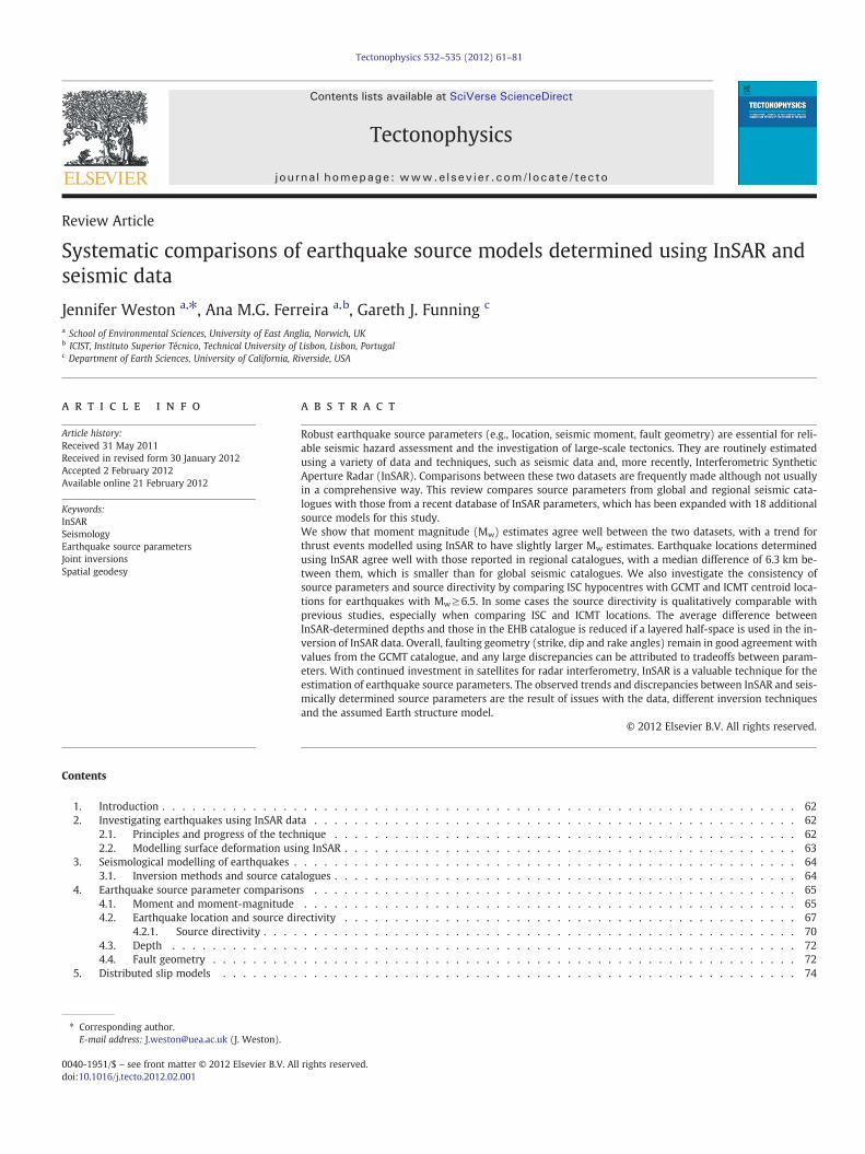
Fig. 4. Difference between InSAR centroid locations and 48 GCMT (Top) solutions, 50 regional seismic solutions (Middle; see also Section 2.2) and 46 ISC solutions (Bottom). Thearrows are of constant size and are not to scale; they begin at the InSAR location and point in the direction of the seismic location where the distance in kilometres between the twolocations is indicated by the colour of the arrow. The median difference for comparisons with GCMT is 16.96 km (σ=10.74 km), for regional catalogues the median is 6.26 km(σ=6.49 km), and a median of 9.23 km (σ=4.07 km) is obtained for comparisons with the ISC catalogue. It must be noted that all comparisons in this figure are only for earth-quakes with regional solutions.

68 J. Weston et al. / Tectonophysics 532–535 (2012) 61–81

seismic estimates using the updated database show the locations todiffer by 21.0 km (σ=12.7 km), 11.6 km (σ=6.9 km) and 9.3 km(σ=7.5 km) for GCMT centroid locations, and EHB and ISC hypocen-tre locations, respectively.

Generally, large disagreements are the result of poor quality InSARdata, showing for example decorrelation due to steep topography andpossibly snow in the mountainous areas (e.g., for the Zarand earth-quake, Mw 6.5, 22nd February 2005; Talebian et al., 2006). However,another cause of discrepancies is believed to be the use of simplifiedEarth models in seismic inversions. A good illustration of this is the

systematic westward bias in locations of subduction zone earthquakesoff the coast of South America by seismic catalogues (Pritchard et al.,2006; Weston et al., 2011). If the 3D variations in the velocity structureof subduction zones are taken into accountwhen inverting seismic data,then the hypocentres can shift by up to 25 km (Syracuse and Abers,2009).

Ferreira et al. (2011) found a similar trend for three events off thecoast of Northern Chile in 1993, 1996 and 1998. Four different Earthmodels were tested and in some instances the disagreement betweenInSAR and CMT centroid locations was reduced by up to 40 km. Two

34.5

34.6

34.7

−116.5 −116.4 −116.3 −116.2 −116.1

Longitude (°)

Latit

ude

(°)

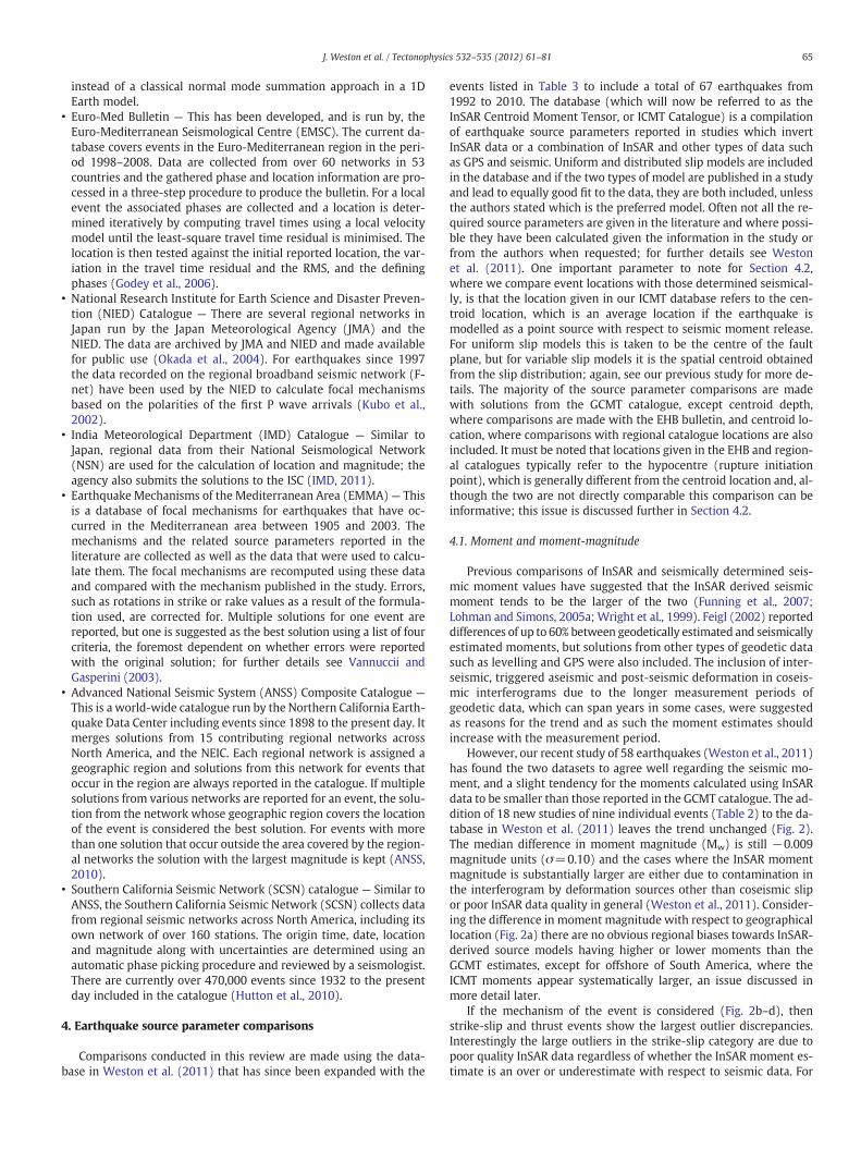
Fig. 5. Locations from InSAR and seismic data for the Hector Mine earthquake with re-spect to geological information. ICMT1 refers to the InSAR study Jonsson et al. (2002),ICMT2 refers to Salichon et al. (2004) and ICMT3 is Simons et al. (2002). SCSN is thehypocentre location from the SCSN catalogue. EHB, ISC and GCMT are the locationsfrom these global catalogues. Mapped fault lines in red correspond to faults that haveexperienced movement in the past 150 years and the yellow lines are for faults youn-ger than 15,000 years; they were plotted using Quaternary fault maps from the UnitedStates Geological Survey (California Geological Survey) (2006).

a

−50 −45 −40 −35 −30 −25 −20 −15 −10−50

−40

−30

−20

−10

0

10

20

East (km)

No

rth

(km

)

ICMTGCMTISCEHBSCSN

b

100

20

0

5

10

15

Dep

th (

km)

Slip

(m

)

2

4

6

8

69J. Weston et al. / Tectonophysics 532–535 (2012) 61–81

forward modelling techniques for the computation of synthetic seis-mograms were also considered but produced similar results for thesame Earth model. However, these events were an isolated case andoverall the use of different Earth models in the GCMT method didlittle to change the distances between the InSAR and GCMT centroid

34.1

34.2

34.3

34.4

34.5

34.6

34.7

34.8

−117.0 −116.8 −116.6 −116.4 −116.2 −116.0

Longitude (°)

Latit

ude

(°)

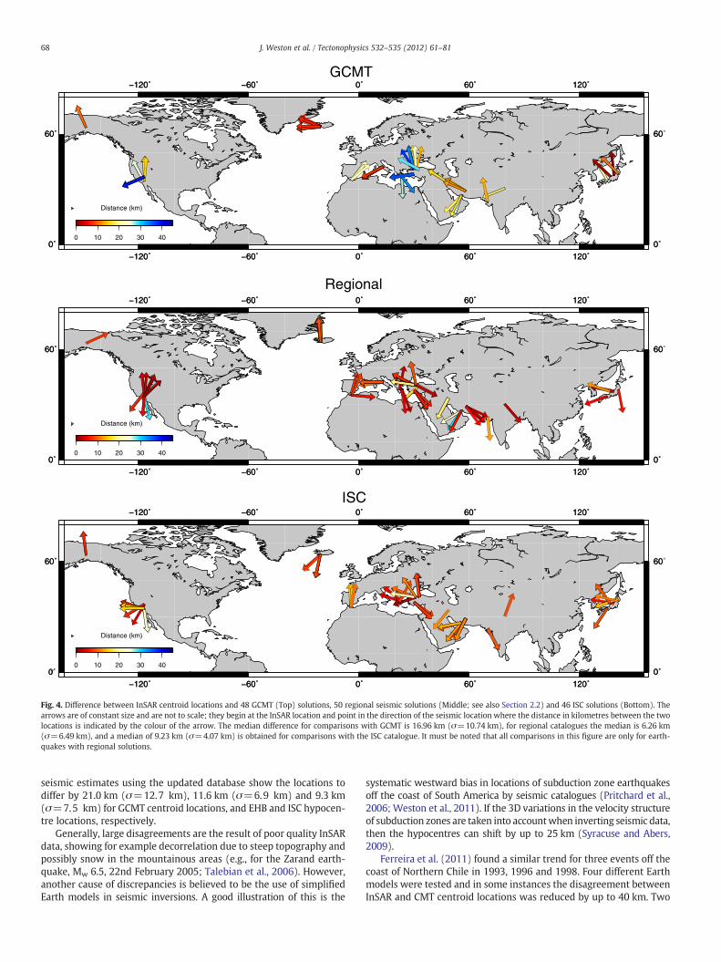
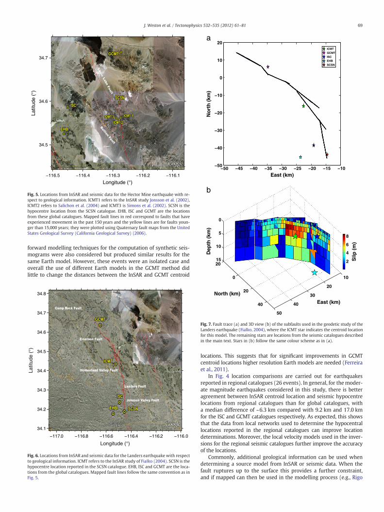
Fig. 6. Locations from InSAR and seismic data for the Landers earthquake with respectto geological information. ICMT refers to the InSAR study of Fialko (2004). SCSN is thehypocentre location reported in the SCSN catalogue. EHB, ISC and GCMT are the loca-tions from the global catalogues. Mapped fault lines follow the same convention as inFig. 5.

50

40

30

20

40

20

East (km)

North (km)

Fig. 7. Fault trace (a) and 3D view (b) of the subfaults used in the geodetic study of theLanders earthquake (Fialko, 2004), where the ICMT star indicates the centroid locationfor this model. The remaining stars are locations from the seismic catalogues describedin the main text. Stars in (b) follow the same colour scheme as in (a).

locations. This suggests that for significant improvements in GCMTcentroid locations higher resolution Earth models are needed (Ferreiraet al., 2011).

In Fig. 4 location comparisons are carried out for earthquakesreported in regional catalogues (26 events). In general, for the moder-ate magnitude earthquakes considered in this study, there is betteragreement between InSAR centroid location and seismic hypocentrelocations from regional catalogues than for global catalogues, witha median difference of ~6.3 km compared with 9.2 km and 17.0 kmfor the ISC and GCMT catalogues respectively. As expected, this showsthat the data from local networks used to determine the hypocentrallocations reported in the regional catalogues can improve locationdeterminations. Moreover, the local velocity models used in the inver-sions for the regional seismic catalogues further improve the accuracyof the locations.

Commonly, additional geological information can be used whendetermining a source model from InSAR or seismic data. When thefault ruptures up to the surface this provides a further constraint,and if mapped can then be used in the modelling process (e.g., Rigo

70 J. Weston et al. / Tectonophysics 532–535 (2012) 61–81

et al., 2004). Alternatively, slip measurements observed in the field(e.g., Hao et al., 2009) can be compared with displacements fromInSAR data. Considering the fine spatial resolution of InSAR data, itis interesting to compare InSAR and seismically determined earth-quake locations with the existing knowledge of geologically mappedsurface offsets in an area. Here we focus on two events in SouthernCalifornia; Hector Mine (Mw 7.1, 16th October 1999) and Landers(Mw 7.3, 28th June 1992). In Figs. 5 and 6, mapped locations of thefaults known to have ruptured in the two earthquakes are comparedwith locations from seismic catalogues and InSAR studies. For HectorMine (Fig. 5), the rupture initiated on a strand of the Lavic Lake fault,approximately at the SCSN location is, yet the EHB and ISC hypocentrelocations are ~18 km to the west of this. A maximum right lateral slipof 5.25 m was observed 4 km south of the epicentre (Treiman et al.,2002), which agrees well with the InSAR centroid locations. The ma-jority of the rupture occurred on the Lavic Lake fault as it propagatednorth-west, which may explain why the GCMT catalogue centroid es-timate is 14–17 km north of the ICMT locations and ~9 km from themapped Lavic Lake fault. Interestingly the ICMT locations are all onthe west side of the mapped fault yet for two of the three InSAR solu-tions (Jonsson et al., 2002; Salichon et al., 2004) the fault dips to theeast, in agreement with the solution in the GCMT catalogue. Thisissue and the slip distribution of the three InSAR solutions are dis-cussed further in Section 5.1.

The Landers earthquake (Fig. 6) was larger than the Hector Mineevent and involved five different faults with a total rupture lengthof ~80 km (Sieh et al., 1993). The agreement between the locationof mapped faults and earthquake locations is better than for HectorMine. The event is believed to have initiated on the Johnson Valleyfault, as indicated by the SCSN location in Fig. 6, which also showsthe ISC and EHB again to the west, by ~8 km. The GCMT is the mostnortherly location, slightly to the east of the Emerson fault, whereasthe ICMT location (calculated from the InSAR model of Fialko(2004) is to the west of the fault zone near the central part of theHomestead Valley fault. This east–west difference in location is inagreement with the fact that the ICMT and GCMT solutions dip in op-posite directions. Locations from the other three seismic cataloguessuggest that the fault dips to the west rather than the east, in agree-ment with InSAR. Large offsets of more than 4 m were observed inthe field on the Emerson fault in the north (Sieh et al., 1993) andslip distribution models from strong motion data showed morethan 6 m of shallow slip on the Camp Rock and Emerson faults (e.g.Cohee and Beroza, 1994; Cotton and Campillo, 1995). However, prob-ably due to these large surface displacements the interferograms areheavily decorrelated near the fault trace, so despite the use of azi-muth offsets, the resulting slip distribution from these InSAR dataappear to estimate much lower values of slip on the same faults. Con-sequently the maximum slip is nearer the middle of the rupturelength in the InSAR derived finite fault model (Fig. 7) and the result-ing ICMT centroid location is further south than the GCMT location.Furthermore, even though the GCMT location appears consistentwith this maximum slip at the northern end of the rupture, ~50% ofthe moment is still estimated to have been released on the Home-stead Valley fault (Cohee and Beroza, 1994). Therefore, errors in theassumed Earth model may also be affecting the GCMT location.

Despite this difference between the ICMT and GCMT centroid loca-tions, when compared with hypocentre estimates from various seis-mic catalogues they both indicate rupture propagation towards thenorth. This is in agreement with rupture models calculated for thisevent (e.g. Cohee and Beroza, 1994; Wald and Heaton, 1994).

4.2.1. Source directivityComparisons of hypocentre and centroid locations can provide in-

formation regarding the rupture length and directivity. A previouscomparison of ISC hypocentre locations and GCMT centroid locationsshowed that while for earthquakes with Mw≥6.5 these comparisons

provide useful information, for smaller earthquakes the difference be-tween the two can be heavily influenced by location errors, which arelikely due to uncertainty in the assumed Earth models (Smith andEkstrom, 1997). Taking this into account, Fig. 8 compares ISC hypo-centre locations with GCMT and ICMT centroid locations for eventswith Mw≥6.5. It could be argued that for events larger than this,there are still significant errors associated with the locations reportedin the GCMT and ISC catalogue (Weston et al., 2011). However, thehypocentre-centroid distances being considered here are on averagelarger than the errors previously found for ISC hypocentre locations;~9 km in this study and ~3–16 km reported in (Syracuse and Abers,2009). Also we are not using the differences between ISC and GCMTor ICMT locations as a means of definitively calculating the rupturelength and direction, but rather to qualitatively investigate the consis-tency of results obtained using different centroid locations. Globallythe distances between ISC hypocentres and ICMT and GCMT centroidlocations are similar, with median distances of ~32 km and ~42 km,respectively. The orientations of hypocentre-centroid vectors show amixed pattern globally (Fig. 8), where for some earthquakes thereis good agreement with rupture directions from previous individualstudies. For example, the Denali earthquake (Mw 7.9, 3rd November2002) shows the largest difference between hypocentre and centroidlocation (~180 km), with the ICMT and GCMT centroids being in agree-ment with the unilateral south-east rupture models from various seis-mic and geodetic studies (e.g. Asano et al., 2005; Velasco et al., 2004).However, there are significant disagreements for several other events,as will now be discussed.

As one might expect from previous work (e.g. Weston et al., 2011),some earthquakes in the south American subduction zone show in-consistency between ICMT and GCMT centroid locations in relationto the ISC hypocentre. One of the largest discrepancies is in relationto three earthquakes in the northern Chile subduction zone; Mw 6.8,11th July 1993, Mw 6.7, 19th April 1996, and Mw 7.1, 30th January1998 (NC93, NC96 and, NC98 in Fig. 8c–d, respectively). The ICMTlocations are relatively close to the hypocentre (4–13 km) whereasthe GCMT locations are systematically located ~50 km to the west(Fig. 8c–d). As previously mentioned, this bias is thought to be the re-sult of errors in assumed Earth models, so this systematic direction isunlikely to reflect the true rupture directivity.

In the same region there is also disagreement between ISC-ICMTand ISC-GCMT vectors for the Nazca Ridge earthquake (Mw 7.7, 12thNovember 1996, NR in Fig. 8c–d). The ICMT centroid location istwice as far away from the ISC hypocentre than the GCMT, but sug-gests a directivity in better agreement with the initial south eastalong-strike rupture propagation reported by Swenson and Beck(1999). It must be noted though that for the remaining earthquakesin this region there is general good agreement between reported rup-ture directivity and the ISC-ICMT and ISC-GCMT location vectors: An-tofagasta (Mw 8.1, 30th July 1995, AN), Aiquile (Mw 6.5, 22nd May1998, AI), Arequipa (Mw 8.1, 23rd June 2001, AR), Pisco (Mw 8.1,15th August 2007, PI), and Tocopilla (Mw 7.8, 14th November 2007,TO).

The ISC-ICMT location vectors also appear to disagree significantlywith the ISC-GCMT vectors for three events in the North Anatolianfault zone in Turkey. For example, if we consider these locationsand a distributed slip model (Fig. 9) for the Izmit earthquake (Mw

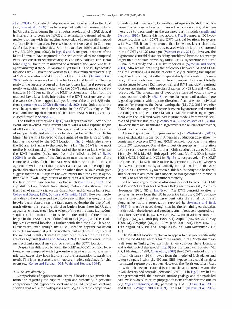
7.5, 17th August 1999; Cakir et al., 2003) the GCMT centroid is a sig-nificant distance (~30 km) away from the modelled fault planes andwhen compared with the ISC and EHB hypocentres could imply anorthward rupture propagation. However, the North Anatolian Faulton which this event occurred is not north–south trending and theInSAR-determined centroid locations (ICMT 1–3 in Fig. 9) are in bet-ter agreement with the observed surface geology and the modelledeast–west bilateral rupture propagation from various seismic studies(e.g. Yagi and Kikuchi, 2000), particularly ICMT1 (Cakir et al., 2003)and ICMT2 (Wright, 2000) (Fig. 9). The ICMT3 (Delouis et al., 2002)

0 50 100 150 200

Distance (km)

GCMT

0 50 100 150 200

Distance (km)

ICMT

AI

PI

TOAN

NC93NC96NC98NC98

NRAR

GCMT

AI

PI

TOAN

NC93

NC96

NC98

NRAR

ICMT

a

c d

b

Fig. 8. Fourmaps illustrating comparisons between ISC hypocentre locations and GCMT centroid locations (a) and ICMT centroid locations (b) for 28 earthquakes; the ICMT comparisonshavemore arrows due to multiple InSAR studies for the same earthquake. All the arrows are the same size (not to real scale) and begin at the ISC location and point towards the centroidlocationwhere the colour of the arrow indicates the distance between the two locations. c) This is a zoomed-inmapof ISC hypocentre andGCMT centroid locations for nine earthquakes inthe South American region, d) is the same as c) except that it shows ICMT centroid locations instead. The labels next to each arrow refer to the name of the event where: AI = Aiquile,Bolivia; AN = Antofagasta, Chile; AR = Arequipa, Peru; NC93, NC96, NC98 = North Chile Subduction Zone 1993, 1996 and 1998, respectively; NR = Nazca Ridge, Peru; PI = Pisco,Peru, and TO = Tocopilla, Chile. See text for more details.

71J. Weston et al. / Tectonophysics 532–535 (2012) 61–81

050

100150

0

5

10

15

20

25

30

35

0

20

40

North(km)

East (km)

Dep

th (k

m)

Slip

(m

)

0

2

4

ICMT1ICMT2ICMT3GCMTISCEHB

Fig. 9. Distributed slipmodel for the Izmit earthquake, fromCakir et al. (2003),where ICMT1indicates the centroid location for this model. ICMT2 and ICMT3 refer to centroid locationsfrom the studies of Wright (2000) and Delouis et al. (2002), respectively. The remaining lo-cations are from seismic catalogues described in the main text (see figure legend).

0

10

0 10 20 30 40 50 60

DepthEHB (km)

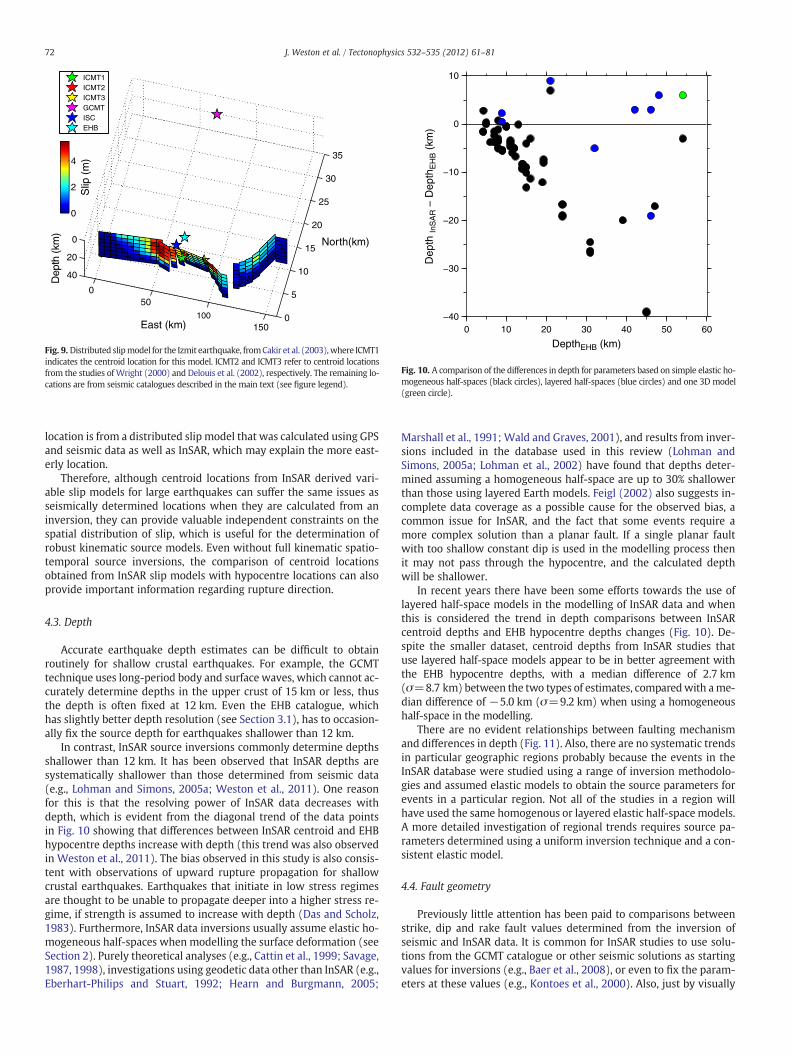
Fig. 10. A comparison of the differences in depth for parameters based on simple elastic ho-mogeneous half-spaces (black circles), layered half-spaces (blue circles) and one 3D model(green circle).

72 J. Weston et al. / Tectonophysics 532–535 (2012) 61–81

location is from a distributed slip model that was calculated using GPSand seismic data as well as InSAR, which may explain the more east-erly location.

Therefore, although centroid locations from InSAR derived vari-able slip models for large earthquakes can suffer the same issues asseismically determined locations when they are calculated from aninversion, they can provide valuable independent constraints on thespatial distribution of slip, which is useful for the determination ofrobust kinematic source models. Even without full kinematic spatio-temporal source inversions, the comparison of centroid locationsobtained from InSAR slip models with hypocentre locations can alsoprovide important information regarding rupture direction.

4.3. Depth

Accurate earthquake depth estimates can be difficult to obtainroutinely for shallow crustal earthquakes. For example, the GCMTtechnique uses long-period body and surface waves, which cannot ac-curately determine depths in the upper crust of 15 km or less, thusthe depth is often fixed at 12 km. Even the EHB catalogue, whichhas slightly better depth resolution (see Section 3.1), has to occasion-ally fix the source depth for earthquakes shallower than 12 km.

In contrast, InSAR source inversions commonly determine depthsshallower than 12 km. It has been observed that InSAR depths aresystematically shallower than those determined from seismic data(e.g., Lohman and Simons, 2005a; Weston et al., 2011). One reasonfor this is that the resolving power of InSAR data decreases withdepth, which is evident from the diagonal trend of the data pointsin Fig. 10 showing that differences between InSAR centroid and EHBhypocentre depths increase with depth (this trend was also observedin Weston et al., 2011). The bias observed in this study is also consis-tent with observations of upward rupture propagation for shallowcrustal earthquakes. Earthquakes that initiate in low stress regimesare thought to be unable to propagate deeper into a higher stress re-gime, if strength is assumed to increase with depth (Das and Scholz,1983). Furthermore, InSAR data inversions usually assume elastic ho-mogeneous half-spaces when modelling the surface deformation (seeSection 2). Purely theoretical analyses (e.g., Cattin et al., 1999; Savage,1987, 1998), investigations using geodetic data other than InSAR (e.g.,Eberhart-Philips and Stuart, 1992; Hearn and Burgmann, 2005;

Marshall et al., 1991; Wald and Graves, 2001), and results from inver-sions included in the database used in this review (Lohman andSimons, 2005a; Lohman et al., 2002) have found that depths deter-mined assuming a homogeneous half-space are up to 30% shallowerthan those using layered Earth models. Feigl (2002) also suggests in-complete data coverage as a possible cause for the observed bias, acommon issue for InSAR, and the fact that some events require amore complex solution than a planar fault. If a single planar faultwith too shallow constant dip is used in the modelling process thenit may not pass through the hypocentre, and the calculated depthwill be shallower.

In recent years there have been some efforts towards the use oflayered half-space models in the modelling of InSAR data and whenthis is considered the trend in depth comparisons between InSARcentroid depths and EHB hypocentre depths changes (Fig. 10). De-spite the smaller dataset, centroid depths from InSAR studies thatuse layered half-space models appear to be in better agreement withthe EHB hypocentre depths, with a median difference of 2.7 km(σ=8.7 km) between the two types of estimates, comparedwith ame-dian difference of −5.0 km (σ=9.2 km) when using a homogeneoushalf-space in the modelling.

There are no evident relationships between faulting mechanismand differences in depth (Fig. 11). Also, there are no systematic trendsin particular geographic regions probably because the events in theInSAR database were studied using a range of inversion methodolo-gies and assumed elastic models to obtain the source parameters forevents in a particular region. Not all of the studies in a region willhave used the same homogenous or layered elastic half-space models.A more detailed investigation of regional trends requires source pa-rameters determined using a uniform inversion technique and a con-sistent elastic model.

4.4. Fault geometry

Previously little attention has been paid to comparisons betweenstrike, dip and rake fault values determined from the inversion ofseismic and InSAR data. It is common for InSAR studies to use solu-tions from the GCMT catalogue or other seismic solutions as startingvalues for inversions (e.g., Baer et al., 2008), or even to fix the param-eters at these values (e.g., Kontoes et al., 2000). Also, just by visually

0 10

Depth InSAR EHB (km)

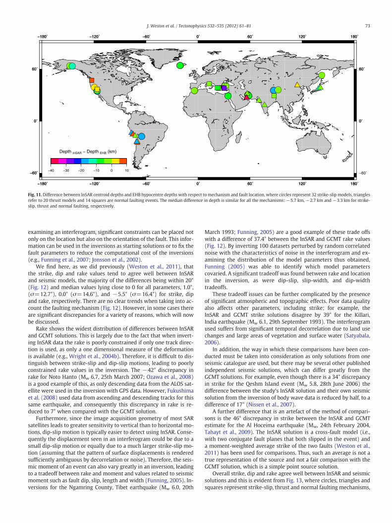
Fig. 11. Difference between InSAR centroid depths and EHB hypocentre depths with respect to mechanism and fault location, where circles represent 32 strike-slip models, trianglesrefer to 20 thrust models and 14 squares are normal faulting events. The median difference in depth is similar for all the mechanisms: −5.7 km, −2.7 km and −3.3 km for strike-slip, thrust and normal faulting, respectively.

73J. Weston et al. / Tectonophysics 532–535 (2012) 61–81

examining an interferogram, significant constraints can be placed notonly on the location but also on the orientation of the fault. This infor-mation can be used in the inversions as starting solutions or to fix thefault parameters to reduce the computational cost of the inversions(e.g., Funning et al., 2007; Jonsson et al., 2002).

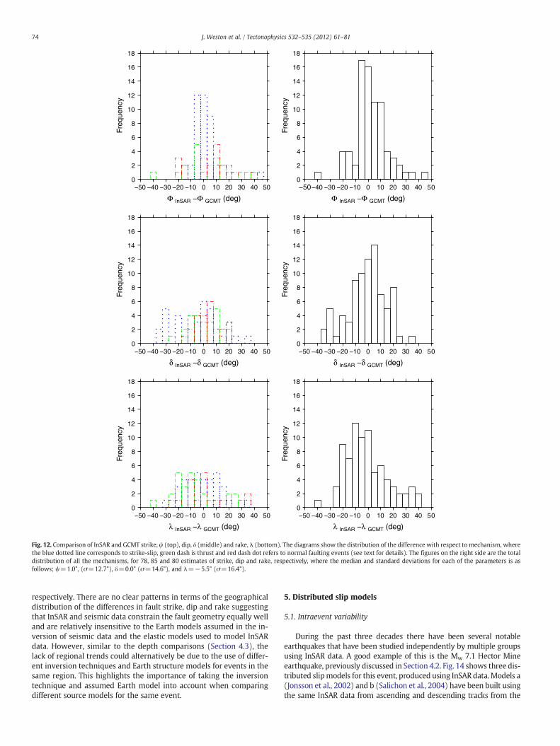
We find here, as we did previously (Weston et al., 2011), thatthe strike, dip and rake values tend to agree well between InSARand seismic models, the majority of the differences being within 20°(Fig. 12) and median values lying close to 0 for all parameters, 1.0°,(σ=12.7°), 0.0° (σ=14.6°), and −5.5° (σ=16.4°) for strike, dipand rake, respectively. There are no clear trends when taking into ac-count the faulting mechanism (Fig. 12). However, in some cases thereare significant discrepancies for a variety of reasons, which will nowbe discussed.

Rake shows the widest distribution of differences between InSARand GCMT solutions. This is largely due to the fact that when invert-ing InSAR data the rake is poorly constrained if only one track direc-tion is used, as only a one dimensional measure of the deformationis available (e.g., Wright et al., 2004b). Therefore, it is difficult to dis-tinguish between strike-slip and dip-slip motions, leading to poorlyconstrained rake values in the inversion. The −42° discrepancy inrake for Noto Hanto (Mw 6.7, 25th March 2007; Ozawa et al., 2008)is a good example of this, as only descending data from the ALOS sat-ellite were used in the inversion with GPS data. However, Fukushimaet al. (2008) used data from ascending and descending tracks for thissame earthquake, and consequently this discrepancy in rake is re-duced to 7° when compared with the GCMT solution.

Furthermore, since the image acquisition geometry of most SARsatellites leads to greater sensitivity to vertical than to horizontal mo-tions, dip-slip motion is typically easier to detect using InSAR. Conse-quently the displacement seen in an interferogram could be due to asmall dip-slip motion or equally due to a much larger strike-slip mo-tion (assuming that the pattern of surface displacements is renderedsufficiently ambiguous by decorrelation or noise). Therefore, the seis-mic moment of an event can also vary greatly in an inversion, leadingto a tradeoff between rake and moment and values related to seismicmoment such as fault dip, slip, length and width (Funning, 2005). In-versions for the Ngamring County, Tibet earthquake (Mw 6.0, 20th

March 1993; Funning, 2005) are a good example of these trade offswith a difference of 37.4° between the InSAR and GCMT rake values(Fig. 12). By inverting 100 datasets perturbed by random correlatednoise with the characteristics of noise in the interferogram and ex-amining the distribution of the model parameters thus obtained,Funning (2005) was able to identify which model parameterscovaried. A significant tradeoff was found between rake and locationin the inversion, as were dip-slip, slip-width, and dip-widthtradeoffs.

These tradeoff issues can be further complicated by the presenceof significant atmospheric and topographic effects. Poor data qualityalso affects other parameters, including strike; for example, theInSAR and GCMT strike solutions disagree by 39° for the Killari,India earthquake (Mw 6.1, 29th September 1993). The interferogramused suffers from significant temporal decorrelation due to land usechanges and large areas of vegetation and surface water (Satyabala,2006).

In addition, the way in which these comparisons have been con-ducted must be taken into consideration as only solutions from oneseismic catalogue are used, but there may be several other publishedindependent seismic solutions, which can differ greatly from theGCMT solutions. For example, even though there is a 34° discrepancyin strike for the Qeshm Island event (Mw 5.8, 28th June 2006) thedifference between the study's InSAR solution and their own seismicsolution from the inversion of body wave data is reduced by half, to adifference of 17° (Nissen et al., 2007).

A further difference that is an artefact of the method of compari-sons is the 46° discrepancy in strike between the InSAR and GCMTestimate for the Al Hoceima earthquake (Mw, 24th February 2004,Tahayt et al., 2009). The InSAR solution is a cross-fault model (i.e.,with two conjugate fault planes that both slipped in the event) anda moment-weighted average strike of the two faults (Weston et al.,2011) has been used for comparisons. Thus, such an average is not atrue representation of the source and not a fair comparison with theGCMT solution, which is a simple point source solution.

Overall strike, dip and rake agree well between InSAR and seismicsolutions and this is evident from Fig. 13, where circles, triangles andsquares represent strike-slip, thrust and normal faulting mechanisms,

0

2

4

6

8

10

12

14

16

18

Freq

uenc

y

0 10 20 30 40 50

Φ InSAR Φ GCMT (deg)

0

2

4

6

8

10

12

14

16

18

Freq

uenc

y

0 10 20 30 40 50

Φ InSAR Φ GCMT (deg)

0

2

4

6

8

10

12

14

16

18

Freq

uenc

y

0 10 20 30 40 50

δ InSAR δ GCMT (deg)

0

2

4

6

8

10

12

14

16

18

Freq

uenc

y

0 10 20 30 40 50

δ InSAR δ GCMT (deg)

0

2

4

6

8

10

12

14

16

18

Freq

uenc

y

0 10 20 30 40 50

λ InSAR λ GCMT (deg)

0

2

4

6

8

10

12

14

16

18

Freq

uenc

y

0 10 20 30 40 50

λ InSAR λ GCMT (deg)

Fig. 12. Comparison of InSAR and GCMT strike, ψ (top), dip, δ (middle) and rake, λ (bottom). The diagrams show the distribution of the difference with respect to mechanism, wherethe blue dotted line corresponds to strike-slip, green dash is thrust and red dash dot refers to normal faulting events (see text for details). The figures on the right side are the totaldistribution of all the mechanisms, for 78, 85 and 80 estimates of strike, dip and rake, respectively, where the median and standard deviations for each of the parameters is asfollows; ψ=1.0°, (σ=12.7°), δ=0.0° (σ=14.6°), and λ=−5.5° (σ=16.4°).

74 J. Weston et al. / Tectonophysics 532–535 (2012) 61–81

respectively. There are no clear patterns in terms of the geographicaldistribution of the differences in fault strike, dip and rake suggestingthat InSAR and seismic data constrain the fault geometry equally welland are relatively insensitive to the Earth models assumed in the in-version of seismic data and the elastic models used to model InSARdata. However, similar to the depth comparisons (Section 4.3), thelack of regional trends could alternatively be due to the use of differ-ent inversion techniques and Earth structure models for events in thesame region. This highlights the importance of taking the inversiontechnique and assumed Earth model into account when comparingdifferent source models for the same event.

5. Distributed slip models

5.1. Intraevent variability

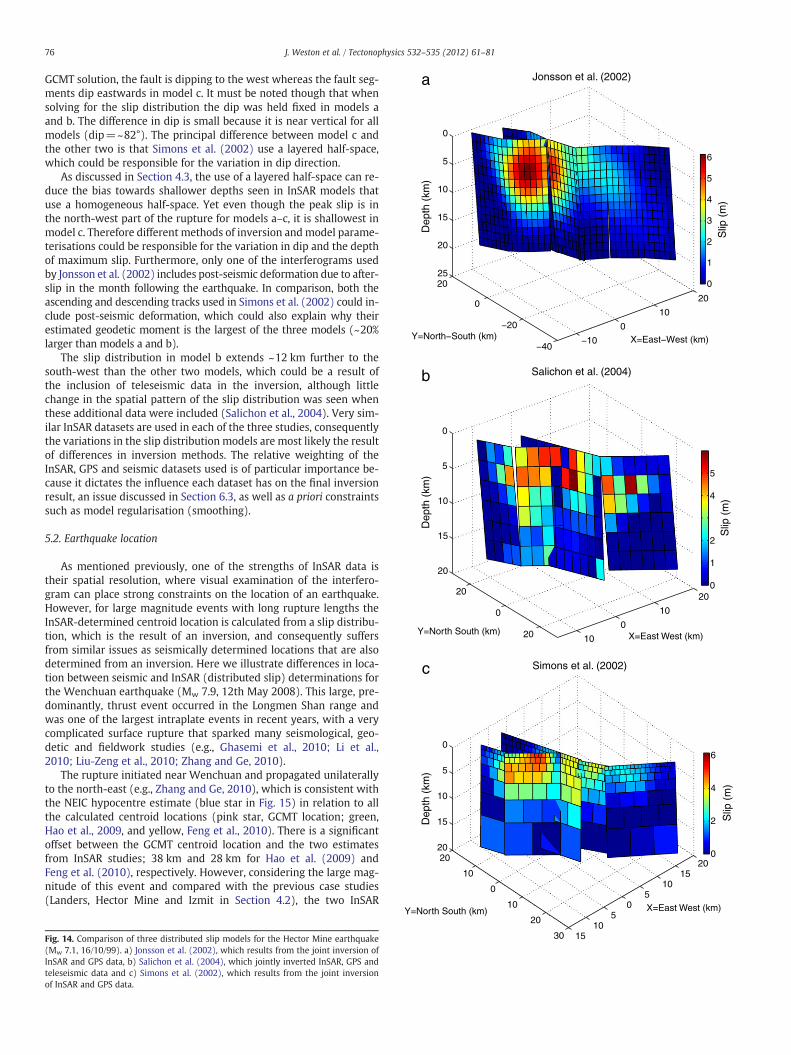
During the past three decades there have been several notableearthquakes that have been studied independently by multiple groupsusing InSAR data. A good example of this is the Mw 7.1 Hector Mineearthquake, previously discussed in Section 4.2. Fig. 14 shows three dis-tributed slipmodels for this event, produced using InSAR data.Models a(Jonsson et al., 2002) and b (Salichon et al., 2004) have been built usingthe same InSAR data from ascending and descending tracks from the

0 10 20 30 40 50

Φ InSAR Φ GCMT (o)

Str

ike

(Φ)

0 10 20 30 40 50

δ InSAR δ GCMT (o)

Dip

(δ)

0 20 40

λ InSAR λ GCMT (o)

Rak

e (λ

)

Fig. 13. Differences, in degrees, between GCMT and InSAR strike, dip and rake with respect to mechanism and InSAR location. The notation for each mechanism is the same as inprevious figures (strike-slip = circle, triangle = thrust, square = normal).

75J. Weston et al. / Tectonophysics 532–535 (2012) 61–81

ERS-1 andERS-2 satellites, to produce interferograms with measure-ment periods of 35 days. Model c (Fig. 11c, Simons et al., 2002), usesan ascending interferogram covering a longer period of ~4 years. Thefault geometry is complex for this event and each study uses multiplefault segments, varying from 4 to 9. Despite the varying numbers of

segments, the length, width, strike and rake values are consistent acrossall the models, likely the result of the fact that the trace of the surfacerupture is well constrained by the InSAR data.

However, there is some discrepancy in the direction of dip, asmentioned in Section 4.2. For the ICMT models a and b, and the

a

0

10

200

20

0

5

10

15

20

25

Jonsson et al. (2002)

Dep

th (

km)

Dep

th (

km)

Slip

(m

)S

lip (

m)

0

1

2

3

4

5

6

b

10

0

10

20

20

0

20

0

5

10

15

20

X=East West (km)

Salichon et al. (2004)

Y=North South (km)

0

1

2

4

5

c

05

1015

20

10

0

10

20

0

5

10

15

20

Simons et al. (2002)

Dep

th (

km)

Slip

(m

)

0

2

4

6

76 J. Weston et al. / Tectonophysics 532–535 (2012) 61–81

GCMT solution, the fault is dipping to the west whereas the fault seg-ments dip eastwards in model c. It must be noted though that whensolving for the slip distribution the dip was held fixed in models aand b. The difference in dip is small because it is near vertical for allmodels (dip=~82°). The principal difference between model c andthe other two is that Simons et al. (2002) use a layered half-space,which could be responsible for the variation in dip direction.

As discussed in Section 4.3, the use of a layered half-space can re-duce the bias towards shallower depths seen in InSAR models thatuse a homogeneous half-space. Yet even though the peak slip is inthe north-west part of the rupture for models a–c, it is shallowest inmodel c. Therefore different methods of inversion andmodel parame-terisations could be responsible for the variation in dip and the depthof maximum slip. Furthermore, only one of the interferograms usedby Jonsson et al. (2002) includes post-seismic deformation due to after-slip in the month following the earthquake. In comparison, both theascending and descending tracks used in Simons et al. (2002) could in-clude post-seismic deformation, which could also explain why theirestimated geodetic moment is the largest of the three models (~20%larger than models a and b).

The slip distribution in model b extends ~12 km further to thesouth-west than the other two models, which could be a result ofthe inclusion of teleseismic data in the inversion, although littlechange in the spatial pattern of the slip distribution was seen whenthese additional data were included (Salichon et al., 2004). Very sim-ilar InSAR datasets are used in each of the three studies, consequentlythe variations in the slip distribution models are most likely the resultof differences in inversion methods. The relative weighting of theInSAR, GPS and seismic datasets used is of particular importance be-cause it dictates the influence each dataset has on the final inversionresult, an issue discussed in Section 6.3, as well as a priori constraintssuch as model regularisation (smoothing).

5.2. Earthquake location

As mentioned previously, one of the strengths of InSAR data istheir spatial resolution, where visual examination of the interfero-gram can place strong constraints on the location of an earthquake.However, for large magnitude events with long rupture lengths theInSAR-determined centroid location is calculated from a slip distribu-tion, which is the result of an inversion, and consequently suffersfrom similar issues as seismically determined locations that are alsodetermined from an inversion. Here we illustrate differences in loca-tion between seismic and InSAR (distributed slip) determinations forthe Wenchuan earthquake (Mw 7.9, 12th May 2008). This large, pre-dominantly, thrust event occurred in the Longmen Shan range andwas one of the largest intraplate events in recent years, with a verycomplicated surface rupture that sparked many seismological, geo-detic and fieldwork studies (e.g., Ghasemi et al., 2010; Li et al.,2010; Liu-Zeng et al., 2010; Zhang and Ge, 2010).

The rupture initiated near Wenchuan and propagated unilaterallyto the north-east (e.g., Zhang and Ge, 2010), which is consistent withthe NEIC hypocentre estimate (blue star in Fig. 15) in relation to allthe calculated centroid locations (pink star, GCMT location; green,Hao et al., 2009, and yellow, Feng et al., 2010). There is a significantoffset between the GCMT centroid location and the two estimatesfrom InSAR studies; 38 km and 28 km for Hao et al. (2009) andFeng et al. (2010), respectively. However, considering the large mag-nitude of this event and compared with the previous case studies(Landers, Hector Mine and Izmit in Section 4.2), the two InSAR

1510

5

30

20X=East West (km)Y=North South (km)

Fig. 14. Comparison of three distributed slip models for the Hector Mine earthquake(Mw 7.1, 16/10/99). a) Jonsson et al. (2002), which results from the joint inversion ofInSAR and GPS data, b) Salichon et al. (2004), which jointly inverted InSAR, GPS andteleseismic data and c) Simons et al. (2002), which results from the joint inversionof InSAR and GPS data.

a

0 50 100 150 200 250 300

0

50

100

150

200

250

East (km)

Nor

th (

km)

ICMT1ICMT2GCMTNEIC

c

50

100

150

200

250

Nor

th (

km)

Slip

(m

)

2

4

6

8

10S

lip (

m)

0

2

4

6

8

10

b

0 50 100 150 200 250 300

0

50

100

150

200

250

East (km)

Nor

th (

km)

77J. Weston et al. / Tectonophysics 532–535 (2012) 61–81

estimates are in good agreement with each other (~22 km), and thedifferences seen are likely due to some discrepancies in the slip distri-bution. In particular the maximum slip is much lower in the modelfrom Feng et al. (2010) (Fig. 15b) ~7 m, compared with ~12 m forHao et al. (2009). The latter study also obtains a larger area of higherslip for the hypocentre at the south-west end of the rupture. Bothmodels use similar InSAR data (ALOS data from tracks 471–477),but Hao et al. (2009) use measurements of offset observed in thefield to help constrain the source model, whereas GPS and InSARdata were used in Feng et al. (2010), which may explain the observeddifference.

There are also large variations in the finite fault models for thisevent that are calculated using seismic data (e.g., Ji and Hayes,2008; Liu-Zeng et al., 2009). Generally both geodetically and seismi-cally determined source models appear to model two large asperities,one near the hypocentre and one ~150 km to the north east ,but theasperity areas and magnitude of slip vary substantially betweenthem. The two InSAR source models have one or two more subfaultsthan are used in the seismically derived source models (e.g. Ji andHayes, 2008) which are in agreement with observed surface ruptures(e.g. Liu-Zeng et al., 2009). The source model from Hao et al. (2009)is more consistent with the high peak slip seen in the seismically de-rived source models and offsets observed in the field (e.g. Liu-Zeng etal., 2009; Nakamura et al., 2010). The large number of varying finitefault models that fit the observed data is potentially due to the com-plicated nature of the rupture. Despite this complexity, the relativegood agreement in centroid location between the two InSAR studiesdemonstrates the ability of InSAR to constrain the spatial features ofthe rupture.

6. Discussion and conclusions

6.1. Source parameter validation

Seismic and InSAR data are independent observations of differentaspects of an earthquake, therefore with our compilation of sourceparameters from published InSAR studies, it is possible to validatesource parameters from seismic catalogues against an independentdataset. Comparisons between databases compiled using InSAR andseismic catalogues have highlighted certain issues. For example, thecomparisons of GCMT and InSAR centroid locations have highlightedlimitations in the GCMT location, as well as the influence that theEarth model used in CMT inversions has on the location of the events(Ferreira et al., 2011). Conversely, the good agreement betweenstrike, dip and rake values suggests how well both datasets constrainthese particular parameters.

Comparisons between InSAR and seismic data can be used toquantify uncertainties in source parameters reported in seismic cata-logues or InSAR studies. For example, as previously mentioned, the lo-cation from the GCMT catalogue varies on average by about 21 kmfrom the InSAR centroid location (Weston et al., 2011). The momentmagnitude differs by ~0.01 (σ=0.10) and fault geometry estimates(strike, dip and rake) by ~0°–5° (σ=13°–16°). The standard devia-tions also give an idea of the level of uncertainty associated withthe source parameters determined using various inversion tech-niques with seismic and geodetic data. These uncertainties need tobe taken into account when using earthquake source parameters todetermine for example changes in tectonic stress (e.g., Coulombstress changes; King et al., 1994) in an area, as these are sensitive to

0 50 100 150 200 250 300

0

East (km)

0

Fig. 15. a) Fault trace of the distributed slip model for the Wenchuan earthquake fromFeng et al. (2010), where ICMT1 refers to the centroid location from the same study,ICMT2 is the centroid location from Hao et al. (2009), GCMT is the centroid locationreported in the GCMT catalogue and NEIC is the hypocenter location from the NEIC Pre-liminary Determination of Epicenters (PDE) catalogue. b) Plan view of the Feng et al.(2010) distributed slip model. c) Plan view of the Hao et al. (2009) distributed slipmodel.

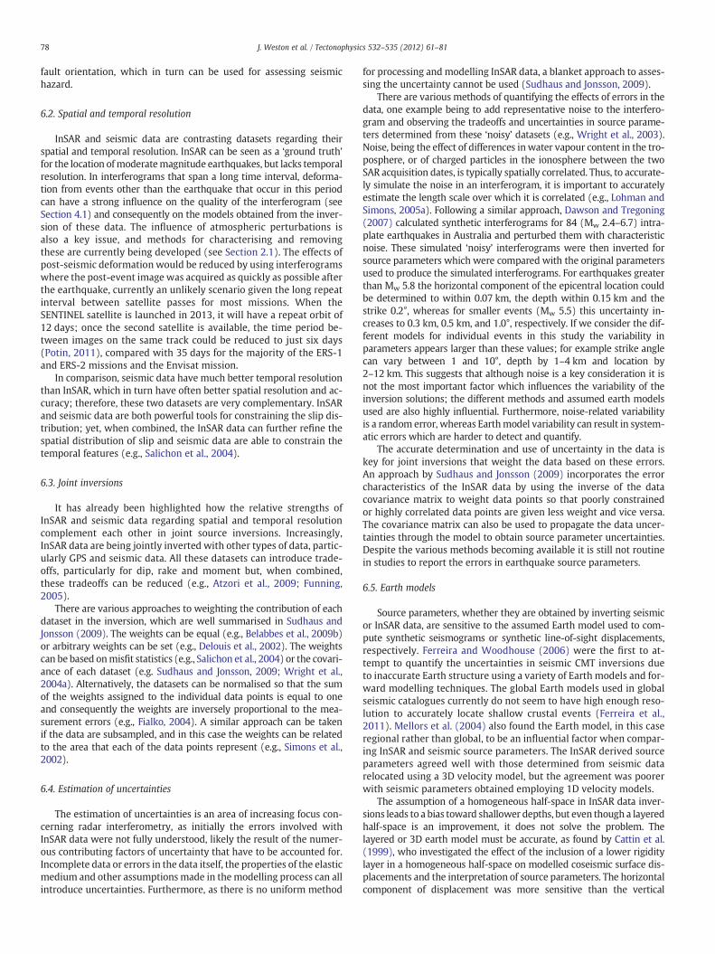
78 J. Weston et al. / Tectonophysics 532–535 (2012) 61–81

fault orientation, which in turn can be used for assessing seismichazard.

6.2. Spatial and temporal resolution

InSAR and seismic data are contrasting datasets regarding theirspatial and temporal resolution. InSAR can be seen as a ‘ground truth’for the location ofmoderatemagnitude earthquakes, but lacks temporalresolution. In interferograms that span a long time interval, deforma-tion from events other than the earthquake that occur in this periodcan have a strong influence on the quality of the interferogram (seeSection 4.1) and consequently on the models obtained from the inver-sion of these data. The influence of atmospheric perturbations isalso a key issue, and methods for characterising and removingthese are currently being developed (see Section 2.1). The effects ofpost-seismic deformation would be reduced by using interferogramswhere the post-event image was acquired as quickly as possible afterthe earthquake, currently an unlikely scenario given the long repeatinterval between satellite passes for most missions. When theSENTINEL satellite is launched in 2013, it will have a repeat orbit of12 days; once the second satellite is available, the time period be-tween images on the same track could be reduced to just six days(Potin, 2011), compared with 35 days for the majority of the ERS-1and ERS-2 missions and the Envisat mission.

In comparison, seismic data have much better temporal resolutionthan InSAR, which in turn have often better spatial resolution and ac-curacy; therefore, these two datasets are very complementary. InSARand seismic data are both powerful tools for constraining the slip dis-tribution; yet, when combined, the InSAR data can further refine thespatial distribution of slip and seismic data are able to constrain thetemporal features (e.g., Salichon et al., 2004).

6.3. Joint inversions

It has already been highlighted how the relative strengths ofInSAR and seismic data regarding spatial and temporal resolutioncomplement each other in joint source inversions. Increasingly,InSAR data are being jointly inverted with other types of data, partic-ularly GPS and seismic data. All these datasets can introduce trade-offs, particularly for dip, rake and moment but, when combined,these tradeoffs can be reduced (e.g., Atzori et al., 2009; Funning,2005).

There are various approaches to weighting the contribution of eachdataset in the inversion, which are well summarised in Sudhaus andJonsson (2009). The weights can be equal (e.g., Belabbes et al., 2009b)or arbitrary weights can be set (e.g., Delouis et al., 2002). The weightscan be based onmisfit statistics (e.g., Salichon et al., 2004) or the covari-ance of each dataset (e.g. Sudhaus and Jonsson, 2009; Wright et al.,2004a). Alternatively, the datasets can be normalised so that the sumof the weights assigned to the individual data points is equal to oneand consequently the weights are inversely proportional to the mea-surement errors (e.g., Fialko, 2004). A similar approach can be takenif the data are subsampled, and in this case the weights can be relatedto the area that each of the data points represent (e.g., Simons et al.,2002).

6.4. Estimation of uncertainties

The estimation of uncertainties is an area of increasing focus con-cerning radar interferometry, as initially the errors involved withInSAR data were not fully understood, likely the result of the numer-ous contributing factors of uncertainty that have to be accounted for.Incomplete data or errors in the data itself, the properties of the elasticmedium and other assumptions made in themodelling process can allintroduce uncertainties. Furthermore, as there is no uniform method

for processing and modelling InSAR data, a blanket approach to asses-sing the uncertainty cannot be used (Sudhaus and Jonsson, 2009).

There are various methods of quantifying the effects of errors in thedata, one example being to add representative noise to the interfero-gram and observing the tradeoffs and uncertainties in source parame-ters determined from these ‘noisy’ datasets (e.g., Wright et al., 2003).Noise, being the effect of differences inwater vapour content in the tro-posphere, or of charged particles in the ionosphere between the twoSAR acquisition dates, is typically spatially correlated. Thus, to accurate-ly simulate the noise in an interferogram, it is important to accuratelyestimate the length scale over which it is correlated (e.g., Lohman andSimons, 2005a). Following a similar approach, Dawson and Tregoning(2007) calculated synthetic interferograms for 84 (Mw 2.4–6.7) intra-plate earthquakes in Australia and perturbed them with characteristicnoise. These simulated ‘noisy’ interferograms were then inverted forsource parameters which were compared with the original parametersused to produce the simulated interferograms. For earthquakes greaterthan Mw 5.8 the horizontal component of the epicentral location couldbe determined to within 0.07 km, the depth within 0.15 km and thestrike 0.2°, whereas for smaller events (Mw 5.5) this uncertainty in-creases to 0.3 km, 0.5 km, and 1.0°, respectively. If we consider the dif-ferent models for individual events in this study the variability inparameters appears larger than these values; for example strike anglecan vary between 1 and 10°, depth by 1–4 km and location by2–12 km. This suggests that although noise is a key consideration it isnot the most important factor which influences the variability of theinversion solutions; the different methods and assumed earth modelsused are also highly influential. Furthermore, noise-related variabilityis a random error, whereas Earthmodel variability can result in system-atic errors which are harder to detect and quantify.

The accurate determination and use of uncertainty in the data iskey for joint inversions that weight the data based on these errors.An approach by Sudhaus and Jonsson (2009) incorporates the errorcharacteristics of the InSAR data by using the inverse of the datacovariance matrix to weight data points so that poorly constrainedor highly correlated data points are given less weight and vice versa.The covariance matrix can also be used to propagate the data uncer-tainties through the model to obtain source parameter uncertainties.Despite the various methods becoming available it is still not routinein studies to report the errors in earthquake source parameters.

6.5. Earth models

Source parameters, whether they are obtained by inverting seismicor InSAR data, are sensitive to the assumed Earth model used to com-pute synthetic seismograms or synthetic line-of-sight displacements,respectively. Ferreira and Woodhouse (2006) were the first to at-tempt to quantify the uncertainties in seismic CMT inversions dueto inaccurate Earth structure using a variety of Earth models and for-ward modelling techniques. The global Earth models used in globalseismic catalogues currently do not seem to have high enough reso-lution to accurately locate shallow crustal events (Ferreira et al.,2011). Mellors et al. (2004) also found the Earth model, in this caseregional rather than global, to be an influential factor when compar-ing InSAR and seismic source parameters. The InSAR derived sourceparameters agreed well with those determined from seismic datarelocated using a 3D velocity model, but the agreement was poorerwith seismic parameters obtained employing 1D velocity models.

The assumption of a homogeneous half-space in InSAR data inver-sions leads to a bias toward shallower depths, but even though a layeredhalf-space is an improvement, it does not solve the problem. Thelayered or 3D earth model must be accurate, as found by Cattin et al.(1999), who investigated the effect of the inclusion of a lower rigiditylayer in a homogeneous half-space on modelled coseismic surface dis-placements and the interpretation of source parameters. The horizontalcomponent of displacement was more sensitive than the vertical

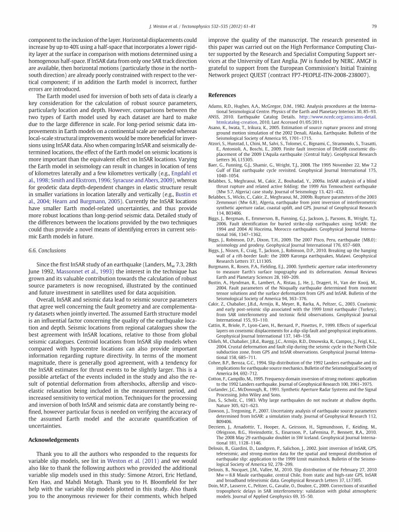
79J. Weston et al. / Tectonophysics 532–535 (2012) 61–81

component to the inclusion of the layer. Horizontal displacements couldincrease by up to 40% using a half-space that incorporates a lower rigid-ity layer at the surface in comparison with motions determined using ahomogenous half-space. If InSAR data from only one SAR track directionare available, then horizontal motions (particularly those in the north–south direction) are already poorly constrained with respect to the ver-tical component; if in addition the Earth model is incorrect, furthererrors are introduced.

The Earth model used for inversion of both sets of data is clearly akey consideration for the calculation of robust source parameters,particularly location and depth. However, comparisons between thetwo types of Earth model used by each dataset are hard to makedue to the large difference in scale. For long-period seismic data im-provements in Earth models on a continental scale are neededwhereaslocal-scale structural improvementswould bemore beneficial for inver-sions using InSAR data. Alsowhen comparing InSAR and seismically de-termined locations, the effect of the Earth model on seismic locations ismore important than the equivalent effect on InSAR locations. Varyingthe Earth model in seismology can result in changes in location of tensof kilometres laterally and a few kilometres vertically (e.g., Engdahl etal., 1998; Smith and Ekstrom, 1996; Syracuse andAbers, 2009),whereasfor geodetic data depth-dependent changes in elastic structure resultin smaller variations in location laterally and vertically (e.g., Bustin etal., 2004; Hearn and Burgmann, 2005). Currently the InSAR locationshave smaller Earth model-related uncertainties, and thus providemore robust locations than long-period seismic data. Detailed study ofthe differences between the locations provided by the two techniquescould thus provide a novel means of identifying errors in current seis-mic Earth models in future.

6.6. Conclusions

Since the first InSAR study of an earthquake (Landers, Mw 7.3, 28thJune 1992, Massonnet et al., 1993) the interest in the technique hasgrown and its valuable contribution towards the calculation of robustsource parameters is now recognised, illustrated by the continuedand future investment in satellites used for data acquisition.

Overall, InSAR and seismic data lead to seismic source parametersthat agree well concerning the fault geometry and are complementa-ry datasets when jointly inverted. The assumed Earth structure modelis an influential factor concerning the quality of the earthquake loca-tion and depth. Seismic locations from regional catalogues show thebest agreement with InSAR locations, relative to those from globalseismic catalogues. Centroid locations from InSAR slip models whencompared with hypocentre locations can also provide importantinformation regarding rupture directivity. In terms of the momentmagnitude, there is generally good agreement, with a tendency forthe InSAR estimates for thrust events to be slightly larger. This is apossible artefact of the events included in the study and also the re-sult of potential deformation from aftershocks, afterslip and visco-elastic relaxation being included in the measurement period, andincreased sensitivity to vertical motion. Techniques for the processingand inversion of both InSAR and seismic data are constantly being re-fined, however particular focus is needed on verifying the accuracy ofthe assumed Earth model and the accurate quantification ofuncertainties.

Acknowledgements

Thank you to all the authors who responded to the requests forvariable slip models, see list in Weston et al. (2011) and we wouldalso like to thank the following authors who provided the additionalvariable slip models used in this study: Simone Atzori, Eric Hetland,Ken Hao, and Mahdi Motagh. Thank you to H. Bloomfield for herhelp with the variable slip models plotted in this study. Also thankyou to the anonymous reviewer for their comments, which helped

improve the quality of the manuscript. The research presented inthis paper was carried out on the High Performance Computing Clus-ter supported by the Research and Specialist Computing Support ser-vices at the University of East Anglia. JW is funded by NERC. AMGF isgrateful to support from the European Commission's Initial TrainingNetwork project QUEST (contract FP7-PEOPLE-ITN-2008-238007).

References

Adams, R.D., Hughes, A.A., McGregor, D.M., 1982. Analysis procedures at the Interna-tional Seismological Centre. Physics of the Earth and Planetary Interiors 30, 85–93.

ANSS, 2010. Earthquake Catalog Details. http://www.ncedc.org/anss/anss-detail.htmlcatalog-creation, 2010, Last Accessed 01/05/2011.

Asano, K., Iwata, T., Irikura, K., 2005. Estimation of source rupture process and strongground motion simulation of the 2002 Denali, Alaska, Earthquake. Bulletin of theSeismological Society of America 95, 1701–1715.

Atzori, S., Hunstad, I., Chini, M., Salvi, S., Tolomei, C., Bignami, C., Stramondo, S., Trasatti,E., Antonioli, A., Boschi, E., 2009. Finite fault inversion of DInSAR coseismic dis-placement of the 2009 L'Aquila earthquake (Central Italy). Geophysical ResearchLetters 36, L15305.

Baer, G., Funning, G.J., Shamir, G., Wright, T.J., 2008. The 1995 November 22, Mw 7.2Gulf of Elat earthquake cycle revisited. Geophysical Journal International 175,1040–1054.

Belabbes, S., Meghraoui, M., Cakir, Z., Bouhadad, Y., 2009a. InSAR analysis of a blindthrust rupture and related active folding: the 1999 Ain Temouchent earthquake(Mw 5.7, Algeria) case study. Journal of Seismology 13, 421–432.

Belabbes, S., Wicks, C., Cakir, Z., Meghraoui, M., 2009b. Rupture parameters of the 2003Zemmouri (Mw 6.8), Algeria, earthquake from joint inversion of interferometricsynthetic aperture radar, coastal uplift, and GPS. Journal of Geophysical Research114, B03406.

Biggs, J., Bergman, E., Emmerson, B., Funning, G.J., Jackson, J., Parsons, B., Wright, T.J.,2006. Fault identification for buried strike-slip earthquakes using InSAR: the1994 and 2004 Al Hoceima, Morocco earthquakes. Geophysical Journal Interna-tional 166, 1347–1362.

Biggs, J., Robinson, D.P., Dixon, T.H., 2009. The 2007 Pisco, Peru, earthquake (M8.0):seismology and geodesy. Geophysical Journal International 176, 657–669.

Biggs, J., Nissen, E., Craig, T., Jackson, J., Robinson, D.P., 2010. Breaking up the hangingwall of a rift-border fault: the 2009 Karonga earthquakes, Malawi. GeophysicalResearch Letters 37, L11305.

Burgmann, R., Rosen, P.A., Fielding, E.J., 2000. Synthetic aperture radar interferometryto measure Earth's surface topography and its deformation. Annual ReviewsEarth and Planetary Sciences 28, 169–209.

Bustin, A., Hyndman, R., Lambert, A., Ristau, J., He, J., Dragert, H., Van der Kooij, M.,2004. Fault parameters of the Nisqually earthquake determined from momenttensor solutions and the surface deformation from GPS and InSAR. Bulletin of theSeismological Society of America 94, 363–376.

Cakir, Z., Chabalier, J.B.d., Armijo, R., Meyer, B., Barka, A., Peltzer, G., 2003. Coseismicand early post-seismic slip associated with the 1999 Izmit earthquake (Turkey),from SAR interferometry and tectonic field observations. Geophysical JournalInternational 155, 93–110.

Cattin, R., Briole, P., Lyon-Caen, H., Bernard, P., Pinettes, P., 1999. Effects of superficiallayers on coseismic displacements for a dip-slip fault and geophysical implications.Geophysical Journal International 137, 149–158.

Chlieh, M., Chabalier, J.B.d., Ruegg, J.C., Armijo, R.D., Dmowska, R., Campos, J., Feigl, K.L.,2004. Crustal deformation and fault slip during the seismic cycle in the North Chilesubduction zone, from GPS and InSAR observations. Geophysical Journal Interna-tional 158, 685–711.

Cohee, B.P., Beroza, G.C., 1994. Slip distribution of the 1992 Landers earthquake and itsimplications for earthquake sourcemechanics. Bulletin of the Seismological Society ofAmerica 84, 692–712.

Cotton, F., Campillo, M., 1995. Frequency domain inversion of strongmotions: applicationto the 1992 Landers earthquake. Journal of Geophysical Research 100, 3961–3975.

Curlander, J.C., McDonough, R., 1991. Synthetic Aperture Radar Systems and the SignalProcessing. John Wiley and Sons.

Das, S., Scholz, C., 1983. Why large earthquakes do not nucleate at shallow depths.Nature 305, 621–623.

Dawson, J., Tregoning, P., 2007. Uncertainty analysis of earthquake source parametersdetermined from InSAR: a simulation study. Journal of Geophysical Research 112,B09406.

Decriem, J., Arnadottir, T., Hooper, A., Geirsson, H., Sigmundsson, F., Keiding, M.,Ofeigsson, B.G., Hreinsdottir, S., Einarsson, P., LaFemina, P., Bennett, R.A., 2010.The 2008 May 29 earthquake doublet in SW Iceland. Geophysical Journal Interna-tional 181, 1128–1146.

Delouis, B., Giardini, D., Lundgren, P., Salichon, J., 2002. Joint inversion of InSAR, GPS,teleseismic, and strong-motion data for the spatial and temporal distribution ofearthquake slip: application to the 1999 Izmit mainshock. Bulletin of the Seismo-logical Society of America 92, 278–299.

Delouis, B., Nocquet, J.M., Vallee, M., 2010. Slip distribution of the February 27, 2010Mw=8.8 Maule earthquake, central Chile, from static and high-rate GPS, InSARand broadband teleseismic data. Geophysical Research Letters 37, L17305.

Doin, M.P., Lasserre, C., Peltzer, G., Cavalie, O., Doubre, C., 2009. Corrections of stratifiedtropospheric delays in SAR interferometry: validation with global atmosphericmodels. Journal of Applied Geophysics 69, 35–50.

80 J. Weston et al. / Tectonophysics 532–535 (2012) 61–81

Dziewonski, A.M., Woodhouse, J.H., 1983. An experiment in systematic study of globalseismicity: centroid-moment tensor solutions for 201 moderate and large earth-quakes of 1981. Journal of Geophysical Research 88, 3247–3271.

Dziewonski, A.M., Woodward, R., 1992. Acoustic imaging on the planetary scale. Acous-tical Imaging 19, 785–797.

Dziewonski, A.M., Chou, T.A., Woodhouse, J.H., 1981. Determination of earthquakesource parameters from waveform data for studies of global and regional seismicity.Journal of Geophysical Research 86, 2825–2852.

Eberhart-Philips, D., Stuart, W., 1992. Material heterogeneity simplifies the picture:Loma Prieta. Bulletin of the Seismological Society of America 82, 1964–1968.

Engdahl, E., van der Hilst, R., Buland, R., 1998. Global teleseismic earthquake relocationwith improved travel times and procedures for depth determination. Bulletin ofthe Seismological Society of America 88, 722–743.

ESA, 2007. Sentinel-1 the radar mission for GMES operational land and sea services.ESA Bulletin 131.

ESA, 2011. ESA's Sentinel Satellites. http://www.esa.int/esaLP/SEMBRS4KXMF_LPgmes_0.html, 2011, Last Accessed, 26/04/11.

Feigl, K.L., 2002. Estimating earthquake source parameters from geodetic measure-ments. International Handbook of Earthquake and Engineering Seismology 81A,1–14.

Feng, G., Hetland, E., Ding, X.L., Li, Z., Zhang, L., 2010. Coseismic fault slip of the 2008Mw 7.9 Wenchuan earthquake estimated from InSAR and GPS measurements.Geophysical Research Letters 37, L01302.

Ferreira, A., Woodhouse, J.H., 2006. Long-period seismic source inversions using globaltomographic models. Geophysical Journal International 166, 1178–1192.

Ferreira, A., Weston, J., Funning, G.J., 2011. Global compilation of interferometric syn-thetic aperture radar earthquake source models: 2. Effects of 3D earth structure.Journal of Geophysical Research 116, B08409.

Fialko, Y., 2004. Probing the mechanical properties of seismically active crust with spacegeodesy: study of the coseismic deformation due to the 1992Mw7.3 Landers (south-ern California) earthquake. Journal of Geophysical Research 109, B03307.

Fukushima, Y., Ozawa, T., Hashimoto, M., 2008. Fault model of the 2007 Noto Hantoearthquake estimated from PALSAR radar interferometry and GPS data. EarthPlanets and Space 60, 99–104.

Funning, G.J., 2005. Source parameters of large shallow earthquakes in the Alpine–Himalayan belt from InSAR and waveform modelling. Ph.D. thesis. Faculty ofPhysical Sciences, University of Oxford.

Funning, G.J., Parsons, B., Wright, T.J., Jackson, J.A., Fielding, E.J., 2005. Surface displace-ments and source parameters of the 2003 Bam (Iran) earthquake from Envisat ad-vanced synthetic aperture radar imagery. Journal of Geophysical Research 110,B09406.

Funning, G.J., Parsons, B., Wright, T.J., 2007. Fault slip in the 1997 Manyi, Tibet earth-quake from linear elastic modelling of InSAR displacements. Geophysical JournalInternational 169, 988–1008.

Ghasemi, H., Fukushima, Y., Koketsu, K., Miyake, H., Wang, Z., Anderson, J.G., 2010.Ground-motion solution simulation for the 2008 Wenchuan. China, earthquakeusing the stochastic finite-fault method. Bulletin of the Seismological Society ofAmerica 100, 2476–2490.

Gilbert, F., Dziewonski, A.M., 1975. An Application of Normal Mode Theory to the Re-trieval of Structural Parameters and Source Mechanisms from Seismic Spectra.Philosophical Transactions of the Royal Society of London.

Godey, A., Bossu, R., Guilbert, J., Mazet-Roux, G., 2006. The Euro-Mediterranean Bulletin:a comprehensive seismological bulletin at regional scale. Seismological ResearchLetters 77, 460–474.

Hao, K.X., Si, H., Fujiwara, H., Ozawa, T., 2009. Coseismic surface-ruptures and crustaldeformations of the 2008 Wenchuan earthquake Mw 7.9, China. Geophysical Re-search Letters 36, L11303.

Hearn, E.H., Burgmann, R., 2005. The effect of elastic layering on inversions of GPS datafor coseismic slip and resulting stress changes: strike-slip earthquakes. Bulletin ofthe Seismological Society of America 95, 1637–1653.

Hergert, T., Heidbach, O., 2006. New insights into the mechanism of postseismic stressrelaxation exemplified by the 23 June 2001, Mw=8.4 earthquake in southernPeru. Geophysical Research Letters 33.

Hutton, K., Woessner, J., Hauksoon, E., 2010. Earthquake monitoring in Southern Cali-fornia for seventy-seven years (1932–2008). Bulletin of the Seismological Societyof America 100, 423–446.

IMD, 2011. Seismological Activities. http://www.imd.gov.in/section/seismo/static/welcome.htm2011Last accessed 23/05/11.

Jeffreys, H., Bullen, K., 1940. Seismological tables. British Association for the Advance-ment of Science 50.

Ji, C., Hayes, G., 2008. Preliminary Result of the May 12, 2008 mw 7.9 Eastern Sichuan,China Earthquake. (Last accessed 19/10/08).

Jonsson, S., Zebker, H., Segall, P., Amelung, F., 2002. Fault slip distribution of the 1999Mw 7.1 Hector Mine, California, earthquake, estimated from satellite radar andGPS measurements. Bulletin of the Seismological Society of America 92,1377–1389.

Jouanne, F., Awan, A., Madji, A., Pecher, A., Latif, M., Kausar, A., Mugnier, J.L., Khan, I.,Khan, N.A., 2011. Postseismic deformation in Pakistan after the 8 October 2005earthquake: evidence of afterslip along a flat north of the Balakot–Bagh thrust.Journal of Geophysical Research 116, B07401.

Kennett, B.L.N., Engdahl, E.R., Buland, R., 1995. Constraints on seismic velocities in theEarth from traveltimes. Geophysical Journal International 122, 108–124.

King, G.C.P., Stein, R., Lin, J., 1994. Static stress changes and the triggering of earth-quakes. Bulletin of the Seismological Society of America 84, 935–953.

Kontoes, C., Elias, P., Sykioti, O., Briole, P., Remy, D., Sachpazi, M., Veis, G., Kotsis, I.,2000. Displacement field and fault model for the September 7, 1999 Athens

earthquake inferred from ERS2 satellite radar interferometry. Geophysical Re-search Letters 27, 3989–3992.

Kubo, A., Fukuyama, E., Kawai, H., Nonomura, K., 2002. NIED seismic moment tensorcatalogue for regional earthquakes around Japan: quality test and application.Tectonophysics 356, 23–48.

Li, Z., Muller, J.P., Cross, P., Fielding, E.J., 2005. Interferometric synthetic aperture radar(InSAR) atmospheric correction: GPS, Moderate Resolution Imaging Spectrora-diometer (MODIS) and InSAR integration. Journal of Geophysical Research 110,B03410.

Li, X.J., Liu, L., Wang, Y.S., Yu, T., 2010. Analysis of horizontal strong-motion attenuationin the great 2008 Wenchuan earthquake. Bulletin of the Seismological Society ofAmerica 100, 2440–2449.

Liu-Zeng, J., Zhang, Z., Wen, L., Tapponnier, P., Sun, J., Xing, X., Hu, G., Xu, Q., Zeng, L.,Ding, L., Ji, C., Hudnut, K.W., van der Woerd, J., 2009. Co-seismic rupture of the12 May 2008, Ms 8.0Wenchuan earthquake, Sichuan: east–west crustal shorteningon oblique, parallel thrusts along the eastern edge of Tibet. Earth and PlanetaryScience Letters 286, 355–370.

Liu-Zeng, J., Wen, L., Sun, J., Zhang, Z., Hu, G., Xing, X., Zeng, L., Xu, Q., 2010. Surface slipand rupture geometry on the Beichuan Fault near Hongkou during the Mw 7.9Wenchuan Earthquake, China. Bulletin of the Seismological Society of America100, 2615–2650.

Lohman, R.B., Simons, M., 2005a. Locations of selected small earthquakes in the Zagrosmountains. Geochemistry, Geophysics, Geosystems 6, Q03001.

Lohman, R.B., Simons, M., 2005b. Some thoughts on the use of InSAR data to constrainmodels of surface deformation: noise structure and data downsampling. Geochemis-try, Geophysics, Geosystems 6, Q01007.

Lohman, R.B., Simons, M., Savage, B., 2002. Location and mechanism of the Little SkullMountain earthquake as constrained by satellite radar interferometry and seismicwaveform modelling. Journal of Geophysical Research 107, B6.

Marshall, G., Stein, R., Tatcher, W., 1991. Faulting geometry and slip from co-seismicelevation changes: the 18 October 1989, Loma Prieta, California, earthquake. Bulle-tin of the Seismological Society of America 81, 1660–1693.

Massonnet, D., Feigl, K.L., 1995. Satellite radar interferometric map of the coseismic de-formation field of the M=6.1 Eureka Valley, California earthquake of May 17,1993. Geophysical Research Letters 22, 1541–1544.

Massonnet, D., Feigl, K.L., 1998. Radar interferometry and its application to changes inthe earth's surface. Reviews of Geophysics 36, 441–500.

Massonnet, D., Rossi, M., Carmona, C., Adragna, F., Peltzer, G., Feigl, K., Rabaute, T., 1993.The displacement field of the Landers earthquake mapped by radar interferometry.Nature 364, 138–142.

McCaffrey, R., Abers, G., Zwick, P., 1991. Inversion of teleseismic bodywaves. In: Lee,W.H.K. (Ed.), IASPEI Software Library, 3, pp. 81–166.

Mellors, R.J., Magistrale, H., Earle, P., Cogbill, A., 2004. Comparison of four moderate-size earthquakes in Southern California using seismology and InSAR. Bulletin ofthe Seismological Society of America 94, 2004–2014.

Motagh, M., Wang, R., Walter, T., Burgmann, R., Fielding, E., Anderssohn, J., Zschau, J.,2008. Coseismic slip model of the 2007 August Pisco earthquake (Peru) as con-strained by Wide Swath radar observations. Geophysical Journal International174, 842–848.

Motagh, M., Schurr, B., Anderssohn, J., Cailleau, B., Walter, T., Wang, R., Vilotte, J.P.,2010. Subduction earthquake deformation associated with 14 November 2007,Mw 7.8 Tocopilla earthquake in Chile: results from InSAR and aftershocks. Tecto-nophysics 490, 60–68.

Nakamura, T., Tsuboi, S., Kaneda, Y., Yamanaka, Y., 2010. Rupture process of the 2008Wenchuan, China earthquake inferred from teleseismic waveform inversion andforward modelling of broadband seismic waves. Tectonophysics 491, 72–84.

Nissen, E., Ghorashi, M., Jackson, J., Parsons, B., Talebian, M., 2007. The 2005 QeshmIsland earthquake (Iran)— a link between buried reverse faulting and surface foldingin the Zagros Simply Folded Belt. Geophysical Journal International 171, 326–338.

Nissen, E., Yamini-Fard, F., Tatar, M., Gholamzadeh, A., Bergman, E., Elliot, J.R., Jackson,J.A., Parsons, B., 2010. The vertical separation of mainshock rupture and microseis-micity at Qeshm Island in the Zagros fold-and-thrust belt, Iran. Earth and PlanetaryScience Letters 296, 181–194.

Okada, Y., 1985. Surface deformation due to shear and tensile fault in a half-space.Bulletin of the Seismological Society of America 75, 1135–1154.

Okada, Y., Kasahara, K., Hori, S., Obara, K., Sekiguchi, S., Fujiwara, H., Yamamoto, A.,2004. Recent progress of seismic observation networks in Japan — Hi-net, F-net,K-NET and KiK-net. Earth Planets and Space 56.

Ozawa, S., Yarai, H., Tobita, M., Une, H., Nishimura, T., 2008. Crustal deformation asso-ciated with the Noto Hanto Earthquake in 2007 in Japan. Earth Planets and Space60, 95–98.

Peltzer, G., Rosen, P., 1995. Surface displacement of the 17 May 1993 Eureka Valley,California, earthquake observed by SAR interferometry. Science 268, 1333–1336.

Perfettini, H., Avouac, J.P., Tavera, H., Kositsky, A., Nocquet, J.M., Bondoux, F., Chlieh, M.,Sladen, A., Audin, L., Farber, D.L., Soler, P., 2010. Seismic and aseismic slip on theCentral Peru megathrust. Nature 465, 78–81.

Pondrelli, S., Morelli, A., Ekstrom, G., Mazza, S., Boschi, E., Dziewonski, A.M., 2002.European–Mediterranean regional centroid-moment tensors: 1997–2000. Physicsof the Earth and Planetary Interiors 130, 71–101.

Pondrelli, S., Salimbeni, S., Morelli, A., Ekstrom, G., Olivieri, M., Boschi, E., 2010. Seismicmoment tensors of the April 2009, L'Aquila (Central Italy) earthquake sequence.Geophysical Journal International 180, 238–242.

Pondrelli, S., Salimbeni, S., Morelli, A., Ekstrom, G., Postpischl, L., Vannuccii, G., Boschi,E., 2011. European–Mediterranean regional centroid moment tensor catalog: solu-tions for 2005–2008. Physics of the Earth and Planetary Interiors 185, 74–81.

Potin, P., 2011. Sentinal-1 Mission Overview. (Last Accessed 26/04/11).

81J. Weston et al. / Tectonophysics 532–535 (2012) 61–81

Pritchard, M.E., Ji, C., Simons, M., 2006. Distribution of slip from 11Mw> 6 earthquake inthe northern Chile subduction zone. Journal of Geophysical Research 111, B10302.

Pussegur, B., Michel, R., Avouac, J.P., 2007. Tropospheric phase delay in interferometricsynthetic aperture radar estimated frommeteorologicalmodelmultispectral imagery.Journal of Geophysical Research 112, B05419.

Rigo, A., de Chabalier, J.B., Meyer, B., Armijo, R., 2004. The 1995 Kozani–Grevena(northern Greece) earthquake revisited: an improved faulting model from syn-thetic radar interferometry. Geophysical Journal International 157, 727–736.

Rosen, P.A., Hensley, S., Joughin, I.R., Li, F.K., Madsen, S.N., Rodriguez, E., Goldtsein, R.M.,2000. Synthetic aperture radar interferometry. Proceedings of the IEEE 88.

Rosen, P.A., Hensley, S., Peltzer, G., 2004. Updated repeat orbit interferometry packagereleased. EOS 85, 47.

Salichon, J., Lundgren, P., Delouis, B., Giardini, D., 2004. Slip history of the 16 October1999 Mw 7.1 Hector Mine Earthquake (California) from the inversion of InSAR,GPS, and teleseismic data. Bulletin of the Seismological Society of America 94,2015–2027.

Satyabala, S.P., 2006. Coseismic ground deformation due to an intraplate earthquakeusing synthetic aperture radar interferometry: the Mw 6.1 Killari, India, earth-quake of 29 September 1993. Journal of Geophysical Research 111, B02302.

Satyabala, S.P., Bilham, R., 2006. Surface deformation and subsurface slip of the 28March 1999 Mw=6.4 west Himalayan Chamoli earthquake from InSAR analysis.Geophysical Research Letters 33, L23305.

Savage, J., 1987. Effect of crustal layering upon dislocation modeling. Journal of Geo-physical Research 92, 10595–10600.

Savage, J., 1998. Displacement field for an edge dislocation in a layered half-space. Jour-nal of Geophysical Research 103, 2439–2446.

Schmidt, D.A., Burgmann, R., 2006. InSAR constraints on the source parameters of the2001 Bhuj earthquake. Geophysical Research Letters 33, L02315.

Sieh, K., Jones, L., Hauksoon, E., Hudnut, K., Eberhart-Philips, D., Heaton, T., Hough, S.,Hutton, K., Kanamori, H., Lilje, A., Lindvall, S., McGill, S.F., Mori, J., Rubin, C.,Spotila, J.A., Stock, J., Thio, H.K., Treiman, J.A., Wernicke, B., Zachariasen, J., 1993.Near-field investigations of the Landers earthquake sequence, April to July 1992.Science 260, 171–176.

Simons, M., Fialko, Y., Rivera, L., 2002. Coseismic deformation from the 1999 Mw 7.1Hector Mine, California, Earthquake as inferred from INSAR and GPS observations.Bulletin of the Seismological Society of America 92, 1390–1402.

Smith, G.P., Ekstrom, G., 1996. Improving teleseismic event locations using a three-dimensional Earth model. Bulletin of the Seismological Society of America 86,788–796.

Smith, G.P., Ekstrom, G., 1997. Interpretation of earthquake epicenter and CMT cen-troid locations, in terms of rupture length and direction. Physics of the Earth andPlanetary Interiors 102, 123–132.

Sudhaus, H., Jonsson, S., 2009. Improved source modelling through combined use ofInSAR and GPS under consideration of correlated data errors: application to theJune 2000 Kleifarvatn earthquake Iceland. Geophysical Journal International 176,389–404.

Sun, J., Shen, Z., Xu, X., Burgmann, R., 2008. Synthetic normal faulting of the 9 January2008 Nima (Tibet) earthquake from conventional and along-track SAR interferom-etry. Geophysical Research Letters 35, L22308.

Swenson, J.L., Beck, S.L., 1999. Source characteristics of the 12 November 1996 Mw 7.7Peru subduction zone earthquake. Pure and Applied Geophysics 154, 731–751.

Syracuse, E.M., Abers, G.A., 2009. Systematic biases in subduction zone hypocenters.Geophysical Research Letters 36, L10303.

Tahayt, A., Feigl, K.L., Mourabit, T., Rigo, A., Reilinger, R., McClusky, S., Fadil, A., Berthier, E.,Dorbath, L., Serroukh, M., Gomez, F., Ben Sari, D., 2009. The Al Hoceima (Morocco)earthquake of 24 February 2004, analysis and interpretation of data from ENVISATASAR and SPOT5 validated by ground-based observations. Remote Sensing of theEnvironment 113, 306–316.

Talebian, M., Biggs, J., Bolourchi, M., Copley, A., Ghassemi, A., Ghorashi, M.,Hollingsworth, J., Jackson, J., Nissen, E., Oveisi, B., Priestly, K., Saiidi, A., 2006.The Dahuiyeh (Zarand) earthquake of 2005 February 22 in central Iran: reactiva-tion of an intramountain reverse fault. Geophysical Journal International 164,137–148.

Treiman, J.A., Kendrick, K.J., Bryant, A., Rockwell, T.K., McGill, S.F., 2002. Primary surfacerupture associated with the Mw 7.1 16 October 1999 Hector Mine Earthquake, SanBernardino County, California. Bulletin of the Seismological Society of America 92,1171–1191.

United States Geological Survey (California Geological Survey), 2006. Quaternary Faultand Fold Database for the United States. http://earthquake.usgs.gov/hazards/qfaults, 2006, Last Accessed, 25/02/11.

Vannuccii, G., Gasperini, P., 2003. A database of revised fault plane solutions for Italyand surrounding regions. Computer & Geosciences 29, 903–909.

Velasco, A.A., Ammon, C.J., Farrell, J., Pankow, K., 2004. Rupture directivity of the 3November 2002 Denali Fault Earthquake determined from surface waves. Bulletinof the Seismological Society of America 94, S293–S299.

Wadge, G., Zhu, M., Holley, R.J., James, I.N., Clark, P.A., Wang, C., Woodage, M.J.,2010. Correction of atmospheric delay effects in radar interferometry using anested mesoscale atmospheric model. Journal of Applied Geophysics 84,537–546.

Wald, D., Graves, R., 2001. Resolution analysis of finite fault source inversion using one-and three-dimensional Green's functions 2. Combining seismic and geodetic data.Journal of Geophysical Research 106, 8767–8788.

Wald, D., Heaton, T., 1994. Spatial and temporal distribution of slip for the 1992Landers, California earthquake. Bulletin of the Seismological Society of America84, 668–691.

Walters, R.J., Elliot, J.R., D'Agostino, N., England, P.C., Hunstad, I., Jackson, J.A., Parsons,B., Phillips, R.J., Roberts, G., 2009. The 2009 L'Aquila earthquake (central Italy):a source mechanism and implications for seismic hazard. Geophysical ResearchLetters 36, L17312.

Weston, J., Ferreira, A., Funning, G.J., 2011. Global compilation of InSAR earthquakesource models: 1. Comparisons with seismic catalogs. Journal of Geophysical Re-search 116, B08408.

Wright, T.J., 2000. Crustal Deformation in Turkey from Synthetic Aperture Radar Inter-ferometry. Ph.D. thesis. Faculty of Physical Sciences, University of Oxford.

Wright, T.J., Parsons, B.E., Jackson, J.A., Haynes, M., Fielding, E.J., England, P.C., Clarke,P.J., 1999. Source parameters of the 1 October 1995 Dinar (Turkey) earthquakefrom SAR interferometry and seismic bodywave modelling. Earth and PlanetaryScience Letters 172, 23–37.

Wright, T.J., Lu, Z., Wicks, C., 2003. Source model for the Mw 6.7, 23 October 2002,Nenana Mountain Earthquake (Alaska) from InSAR. Geophysical Research Letters30, 1974.

Wright, T.J., Lu, Z., Wicks, C., 2004a. Constraining the slip distribution and fault geometryof the Mw 7.9, 3 November 2002, Denali Fault Earthquake with interferometricsynthetic aperture radar and global positioning system data. Bulletin of the Seismo-logical Society of America 94, 175–189.

Wright, T.J., Parsons, B.E., Lu, Z., 2004b. Toward mapping surface deformation in threedimensions using InSAR. Geophysical Research Letters 31.

Yagi, Y., Kikuchi, M., 2000. Source rupture process of the Kocaeli, Turkey, earthquake ofAugust 17 1999, obtained by joint inversion of near-field data and telelseismicdata. Geophysical Research Letters 27, 1969–1972.

Zhang, H., Ge, Z., 2010. Tracking the rupture of the 2008 Wenchuan earthquake byusing the relative back-projection method. Bulletin of the Seismological Societyof America 100, 2551–2560.