system dynamics and stress testing - cbr.ru 6 - imf -system dynamics... · objective identify...

SYSTEM DYNAMICS AND STRESS TESTING

Laura ValderramaInternational Monetary Fund

IMF-Bank of Russia WorkshopRecent Developments in Macroprudential Stress Testing

Bank of Russia, 4-5 September, 2018

Outline

Objective System Dynamics Banks Borrowers Non-bank Financial Institutions Macro-feedback Calibration

2

Objective

Objective

Identify shocks and quantify feedback effects that might affect financial stability and the real economy Assess banks’ individual behavior and system-wide dynamics

under different scenarios Examine propagation of shocks within the financial system Measure the impact on credit growth and GDP growth

Facilitate a rapid policy response to shocks Evaluate the impact of changes to bank capital regulation… … and other financial sector policies Liquidity regulation, regulatory treatment of provisions (IFRS 9), NPL

guidance, LTRO, banking system structure

Modeling Approach

ABM

DSGE Stress Testing

VaR

Examine the transmission mechanism of different types of shocks:exogenous risk (scenario) and endogenous risk (firms’ reaction to shocks)

System Dynamics

Key Features

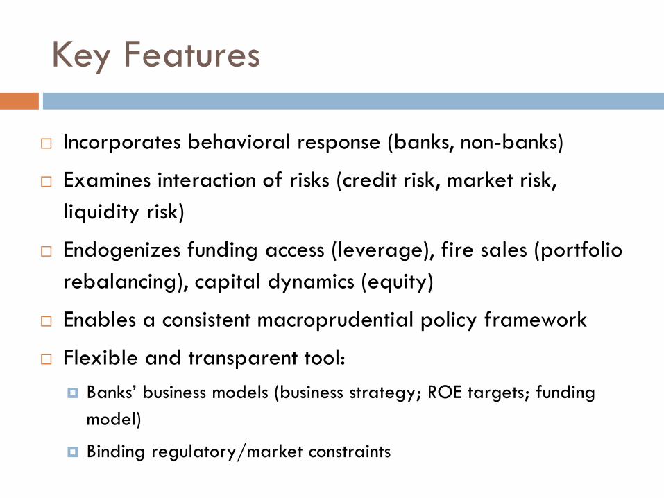
Incorporates behavioral response (banks, non-banks)

Examines interaction of risks (credit risk, market risk, liquidity risk)

Endogenizes funding access (leverage), fire sales (portfolio rebalancing), capital dynamics (equity)

Enables a consistent macroprudential policy framework

Flexible and transparent tool: Banks’ business models (business strategy; ROE targets; funding

model)

Binding regulatory/market constraints

Ingredients

Cournot Nash Equilibrium

BankStrategy

Basel III regulation•Capital•Liquidity•Leverage

MarketLeverage

EndogenousAsset Prices

Macro feedback•Credit growth•GDP growth

Bank i

Securitiesmarkets

Other banks

Equitymarkets

GDP

• At each time step, banks optimize their balance sheet, investors inject/withdraw capital, and noise traders rebalance their asset holdings

• Implications for credit risk, asset volatility, bank capital position, credit growth, GDP growth

Constraint 1: Fundingmarkets

Macro feedback

Constraint 2:RegulatoryFramework

Credit allocation

Leverage

Capital allocation

System Interactions

PDEquity

investors

Noise traders • Lack of

Coordination• Bounded

Rationality

Borrowers

Policy Instruments

Monetary Policy LTRO, TLTRO Forward Guidance Asset purchases/collateral framework

Accounting Policy Provisions

Prudential Capital requirements: structural (min), cyclical (buffers) IRB correlation factor LGD floor Run-off rate (LCR), funding structure (NSFR) Guidance on NPL/write-offs

Banks

Borrowers

Noise Traders

Macroprudential policy LTI, DSTI

Liquidity regulation Redemption policy

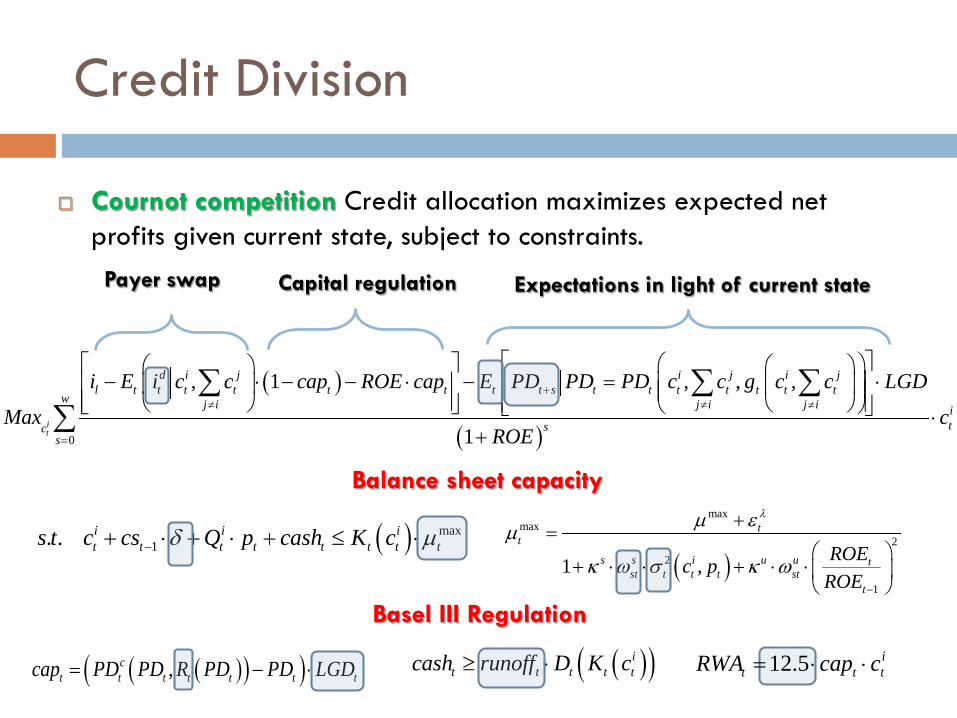
Credit Division

Cournot competition Credit allocation maximizes expected net profits given current state, subject to constraints.

( )

( )0

, 1 , , ,

1it

d i j i j i jl t t t t t t t t s t t t t t t t

w j i j i j i itsc

s

i E i c c cap ROE cap E PD PD PD c c g c c LGD

Max cROE

+≠ ≠ ≠

=

− ⋅ − − ⋅ − = ⋅ ⋅

+

∑ ∑ ∑∑

( ) max1. . i i i

t t t t t t t ts t c cs Q p cash K cδ µ−+ ⋅ + ⋅ + ≤ ⋅

( )( )it t t t tcash runoff D K c≥ ⋅

Balance sheet capacity

Basel III Regulation

( )

maxmax

22

1

1 ,

tt

s s i u u tst t t t st

t

ROEc pROE

λµ εµ

κ ω σ κ ω−

+=

+ ⋅ ⋅ + ⋅ ⋅

( )( )( ),ct t t t t t tcap PD PD R PD PD LGD= − ⋅

ittt ccapRWA ⋅⋅= 5.12

Payer swap Expectations in light of current stateCapital regulation

Credit Policy

Credit allocation

Banks’ underwriting standards define the LTI distribution

Subject to regulatory policy

Credit flow depends on underwriting standards and income

1

i jt t t

jc L L

τ

τ=

= = ⋅∑

( )maxttj

t

LE I

≤ Β

( )j j jt t t

jt t

L E I

such thatτ

= Β ⋅

Β < Β

( )1

i j jt t t t

jc E I

τ

=

= Β ⋅∑

Credit Allocation

14

( ) ( )

( )* **

* ** * * *

* *

*1

1

t tt

t tt t t t

d il t t t t tc cc

td s

dt t t tt ti i i ic c

t t t tc c c c

i i cap ROE cap PD c LGDc

i cap cap PDcap i ROE LGDc c c c

− ⋅ − − ⋅ − ⋅= ∂ ∂ ∂ ∂ ⋅ − − ⋅ + ⋅ + ⋅∂ ∂ ∂ ∂

Capital regulationeffect

Interest margin

Credit risk effect

Expected losses

Funding cost effect

Securities Division

Banks exploit mispricing of securities: (i) securities are measured at fair value (trading book) (ii) banks take into account the cost of capital to cover market risk

where market risk is defined according to Basel IMM approach

and the volatility of asset prices follows an autoregressive process

( )( )max

1

max1

0 t t

i i tt t i t t t t t t t t

ii

t t t t t

if L p

Q p L p K cash cs c if L p L

K cash cs c else

δ

λβ δ δ δβ

λ δ

−

−

> +⋅ = ⋅ − + ⋅ − − ⋅ − − < + < ⋅ − − ⋅ −

( ) 210399.0 tt Gcapmk σ⋅⋅⋅=

( ) ( )21

21

2 /log1 −− ⋅−+⋅= tttt ppθσθσ

( )1dt t t ti capmk ROE capmkδ = ⋅ − + ⋅

Business model

Evolution of Capital

Capital evolves with Dynamic balance sheet (rebalancing of portfolio) Mark-to-market gains/losses in traded securities Net interest income Loan loss provisions (new credit + revision of provisions from credit risk

migration) Investors’ capital flow Dividend payout

If capital falls below the minimum regulatory level Banks continue operating even if their capital falls below regulatory

minimum (benchmark) Banks are forced to be raise capital to satisfy the regulatory minimum

(recapitalization) Credit and dividend payout is constrained (CCB)

Non-Banks

Borrowers

Income distribution

Income linked to growth subject to shocks

The probability of default of borrower j

The probability of default of the portfolio

PD rises with credit growth and declines with growth

( ){ } ( ) ( )j jt t t t t tE I if j E I E Iττ > ⇒ <

( )

1 1j jtt t I tI I gσ ε−= ⋅ + ⋅ +

( ){ }# 1j j l j jt s t s t t t sPD I i L Iδ+ + + = − + ⋅ >

( )1

i i jt t t

jPD c PD

τ

=

= ∑

( ) ( )

0 0

0 0

t ti it t

ct t

t t t t

PD PDandc cPD PDand

E g E g

∂ ∂> >

∂ ∂

∂ ∂< >

∂ ∂

Stochastic

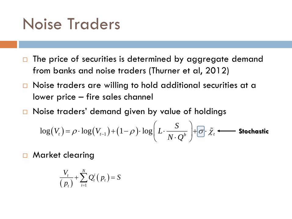
Noise Traders

The price of securities is determined by aggregate demand from banks and noise traders (Thurner et al, 2012)

Noise traders are willing to hold additional securities at a lower price – fire sales channel

Noise traders’ demand given by value of holdings

Market clearing

( ) ( )1

Nitt t

it

V Q p Sp =

+ =∑

( ) ( ) ( )1log log 1 logt t tb

SV V LN Q

ρ ρ σ χ−

= ⋅ + − ⋅ ⋅ + ⋅ ⋅

Stochastic

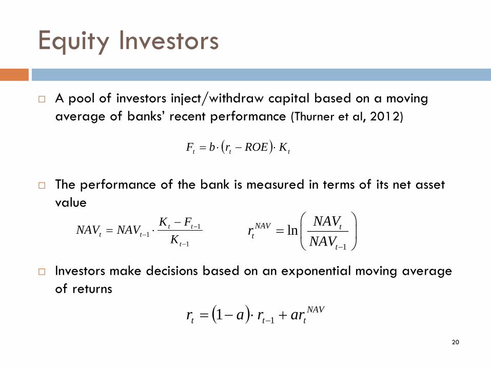
Equity Investors

A pool of investors inject/withdraw capital based on a moving average of banks’ recent performance (Thurner et al, 2012)

The performance of the bank is measured in terms of its net asset value

Investors make decisions based on an exponential moving average of returns

20

( ) ttt KROErbF ⋅−⋅=

( ) NAVttt arrar +⋅−= −11

1

11

−

−−

−⋅=

t

tttt K

FKNAVNAV

1

lnNAV tt

t

NAVrNAV −

=

Macro-feedback

Macro-feedback effects

IS Curve

Expectations Augmented Phillips Curve

Monetary Policy “Taylor-type” Rule

Credit spreads

Interest rates

22

( ) ( ) ( ) ( ) ( ) ( ) yt

ltyttyttyttytt icsNcsNgEgEgE εργβαα +−⋅−⋅⋅⋅+⋅−+⋅= −−+− 2111 /log1

( ) ( ) ( ) ( ) ( ) ππππ εβπαπαπ ttttttttt gEEEE +⋅+⋅−+⋅= +− 11 1

( ) ( )( ) ( )( )[ ] ( ) rttrttr

Tttr

Trt rygEEr εαγππβπρα +⋅−+−⋅+−⋅++⋅= −11*

( ) ( ) ( )( ) ltttl

dtl

lt

dttt

dt

gEymii

sri

εαα

ε

+−⋅−++⋅=

++=

*1

st

t

tttstst rCAR

CARliborss εγαρ +⋅+⋅+⋅= −1Global funding conditionsExcess regulatory capital

Funding costs (policy rate, bank credit spreads)

Lending rates (funding costs, pass-through, borrower credit spreads)

Reduced-form

For the calibration, the following macro-econometric equation is estimated

Key variables: Expected GDP growth

Potential output

Credit growth

23

( ) ( )1 1 2* 1 log / yt y t y y y t t tg g y N cs N csα γ α γ ε− − −= ⋅ + ⋅ + − − ⋅ ⋅ ⋅ +

Calibration

Key Initial Conditions

Credit risk

Macroeconomy

25

5=N Core parameters Balance sheet

Rates Securities market

60=T

0

0

0

0

0

0

0max

max 21 0

183.4157.0

26.410.15

7.336176.0625

11.4%64.351

2524.75 100, 0.0001

t

AcscashrunoffKD

CARRWA

given

λ

µ

µ κ σ

====

===

==

=

= = =

08.004.006.0

0

0

==

=

ROEii

l

l ( )0

0

20

0.9 1900

10000.00010.0001

p LVSσ

σ

= =

===

=

0

0*

0

0

0 0

0.030

0.030.02319.4

0.860.80.1

y

y

gc

y

yny yn

π

ρ

γ

=∆ =

==== ⋅=

=

( )

0

0

1

0.16%4.78%

0.005 0.0056 ln 0.09

0.6

c

PDtt t t t

t

PDPD

N csPD E gN cs

LGD

ε−

=

=

⋅= + ⋅ − + ⋅ =

60=w

983.0=δ

Baseline CAR-at Risk

Adverse Scenarios

GDP shock

Funding (liquidity) shock

Market (liquidity) shock

27

[ ] 02.020,1201.010

−=∈

−==y

t

yt

tiftif

ε

ε

[ ]

<=

∈005.0

20,12t

tifχ

σ

[ ] 460,12 −=∈ λε ttif

GDP shock

-10

-8

-6

-4

-2

0

2

4

6

1 4 7 10 13 16 19 22 25 28 31 34 37 40 43 46 49 52 55 58

Capital Shortfall/GDP

Real GDP - Deviation from Baseline

Real Effects(Percent)

0

2

4

6

8

10

12

14

16

18

20

1 4 7 10 13 16 19 22 25 28 31 34 37 40 43 46 49 52 55 58

CAR CAR min

Bank Solvency(Percent)

• GDP Projections are endogenousto banks’ reaction to stress

• Despite recovery in banks’ capital ratios, permanent real effects

• Recessions deeper and more persistent when second-round effects are included

• Bank recapitalization peaks at 5 percent of nominal GDP

• Over 5-year, cumulative real gdp declines by 8 percent relative to baseline

Funding shock

0

0.05

0.1

0.15

0.2

0.25

0 10 20 30 40 50Baseline Funding Shock

1. Capital Adequacy Ratio(Percent)

18

19

20

21

22

23

24

25


2. Leverage(Assets/Equity)

0

0.5

1

1.5

2

2.5

3

3.5

4

4.5

5


4. GDP Growth(Percent)

-2

-1

0

1

2

3

4

5

6

7

0 10 20 30 40 50

Baseline Funding Shock

3. Credit Growth(Percent)

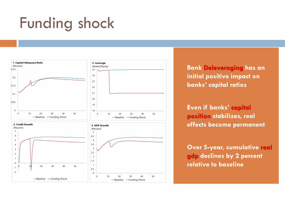
• Bank Deleveraging has an initial positive impact on banks’ capital ratios

• Even if banks’ capital position stabilizes, real effects become permanent

• Over 5-year, cumulative real gdp declines by 2 percent relative to baseline

Market shock

0

0.05

0.1

0.15

0.2

0.25

0 10 20 30 40 50Baseline Market Shock

1. Capital Adequacy Ratio(Percent)

0.8

0.85

0.9

0.95

1


2. Price(Index, Fundamental Value = 1)

22

23

24

25


3. Leverage(Assets/Equity)

0

0.0001

0.0002

0.0003

0.0004

0.0005

0.0006

0.0007

0.0008

0.0009

0.001


4. Price Volatility(Percent)

0

0.5

1

1.5

2

2.5

3

3.5

4

4.5

5


6. GDP Growth(Percent)

0

1

2

3

4

5

6

7

0 10 20 30 40 50

Baseline Market Shock

5. Credit Growth(Percent)

• A MARKET SHOCK (REDEMPTIONS FROM NOISE TRADERS) MORPHS INTO…

• …A LIQUIDITY SHOCK (THROUGH LEVERAGE CONSTRAINT) AND…

• …A CREDIT SHOCK (THROUGH BANKS’ BEHAVIORAL RESPONSE)…

• … INCREASING DEFAULT RISK (THROUGH SECOND-ROUND EFFECTS)…

• …SLOWING DOWN ECONOMIC GROWTH…

• …CUMULATIVE REAL GDP DECLINES BY 1 PERCENT RELATIVE TO BASELINE

Thank you

system dynamics and stress testing - cbr.ru 6 - imf -system dynamics... · objective identify...

Documents