switch-wecc - renewable & appropriate energy...

1

SWITCH-WECC

Data, Assumptions, and Model Formulation

October 2013

Ph.D. Students Josiah Johnston, Ana Mileva, and James H. Nelson

Professor Daniel M. Kammen

Renewable and Appropriate Energy Laboratory (http://rael.berkeley.edu/)

Energy and Resources Group

University of California, Berkeley

2

Table of Contents

1 SWITCH-WECC Model Summary ....................................................................................... 4

1.1 Geographic Scope .................................................................................................... 4

1.2 SWITCH-WECC Capabilities ....................................................................................... 5

1.3 Cost and Fuel Price Inputs ........................................................................................ 6

1.4 Independent Variables ............................................................................................. 8

1.5 Constraints .............................................................................................................. 9

2 Data Description ............................................................................................................ 11

2.1 Load Zones ............................................................................................................ 11

2.1.1 Geospatial Definition .............................................................................................. 11

2.1.2 Cost Regionalization ................................................................................................ 12

2.2 High Voltage Transmission ..................................................................................... 13

2.2.1 General Approach ................................................................................................... 13

2.2.2 De-rating of Thermal Limits to Path Limits ............................................................. 14

2.2.3 Transmission Cost and Terrain Multiplier ............................................................... 15

2.2.4 Transmission Sunk Costs ......................................................................................... 17

2.3 Distribution System ............................................................................................... 17

2.4 Historical Demand Profiles ..................................................................................... 17

2.5 Demand Response Hourly Potentials ...................................................................... 18

2.6 Policies, Initiatives, and Goals ................................................................................ 19

2.6.1 Carbon Cap .............................................................................................................. 19

2.6.2 Renewable Portfolio Standards .............................................................................. 19

2.6.3 California Solar Initiative (CSI) ................................................................................ 20

2.6.4 California Distributed Generation Mandate ........................................................... 20

2.7 Fuel Prices ............................................................................................................. 20

2.8 Biomass Solid Supply Curve .................................................................................... 21

2.9 Existing Generators ................................................................................................ 22

2.9.1 Existing Generator Data .......................................................................................... 22

2.9.2 Existing Hydroelectric and Pumped Hydroelectric Plants ...................................... 23

2.9.3 Existing Wind Plants ................................................................................................ 23

2.10 New Generators and Storage ................................................................................. 24

2.10.1 Capital and O&M Costs ........................................................................................... 24

2.10.2 New Generator and Storage Project Parameters ................................................... 26

2.10.3 Connection Costs .................................................................................................... 26

2.10.4 Non-Renewable Thermal Generators ..................................................................... 28 2.10.4.1 Non-Renewable Thermal Generators without CCS ....................................................................... 28 2.10.4.2 Non-Renewable Thermal Generators with CCS ............................................................................ 28

2.10.5 Compressed Air Energy Storage ............................................................................. 29

2.10.6 Battery Storage ....................................................................................................... 30

2.10.7 Geothermal ............................................................................................................. 30

2.10.8 Biogas and Bioliquid ................................................................................................ 30

3

2.10.9 Biomass Solid .......................................................................................................... 31

2.10.10 Wind and Offshore Wind Resources ................................................................... 31 2.10.10.1 United States Wind ................................................................................................................... 31 2.10.10.2 Canadian Wind .......................................................................................................................... 32

2.10.11 Solar Resources ................................................................................................... 32 2.10.11.1 Distributed Photovoltaics – Residential and Commercial......................................................... 33 2.10.11.2 Central Station Solar – Photovoltaics (PV) and Concentrating Solar Power (CSP) .................... 34

2.10.12 Site Selection of Variable Renewable Projects ................................................... 35

3 SWITCH Investment Model Description .......................................................................... 36

3.1 Study Years, Months, Dates and Hours ................................................................... 36

3.2 Sets and Indices ..................................................................................................... 37

3.3 Decision Variables: Capacity Investment ................................................................ 38

3.4 Decision Variables: Dispatch .................................................................................. 39

3.4.1 Treatment of Operating Reserves .......................................................................... 41

3.5 Objective Function and Economic Evaluation ......................................................... 43

3.6 Constraints ............................................................................................................ 46

3.6.1 Demand-Meeting Constraints ................................................................................ 47

3.6.2 Reserve Margin Constraints .................................................................................... 49

3.6.3 Policy Constraints .................................................................................................... 51

3.6.4 Resource Constraints .............................................................................................. 54

3.6.5 Transmission and Distribution Constraints ............................................................. 56

3.6.6 Operational Constraints .......................................................................................... 58

3.6.7 Demand Response Constraints ............................................................................... 65

3.7 Present-Day Dispatch ............................................................................................. 67

3.8 Post-Investment Dispatch Check ............................................................................ 67

4 References .................................................................................................................... 69

4

1 SWITCH-WECC MODEL SUMMARY

1.1 GEOGRAPHIC SCOPE

This document describes the input data, key assumptions, and linear program formulation of the SWITCH-WECC model. SWITCH is free and open-access software that can be redistributed and modified under the terms of the GNU General Public License version 3. Documentation for the original version of the model created by Dr. Matthias Fripp and applied to California’s power system for his doctoral dissertation can be found at http://www.switch-model.org (Fripp 2008, Fripp 2012).

SWITCH-WECC is a version of the model for the synchronous region of the Western Electricity Coordinating Council (WECC), which extends east-west from the Pacific coast of North America to the eastern border of Colorado, and north-south from the Canadian provinces of British Columbia and Alberta to Arizona and the Mexican state of Baja Mexico Norte. SWITCH-WECC is maintained and developed by Ph.D. students Josiah Johnston, Ana Mileva, and James Nelson in Professor Daniel Kammen’s Renewable and Appropriate Energy Laboratory (RAEL) at the University of California, Berkeley. Previous publications from RAEL include: Nelson et al. 2012; Wei et al. 2012; Wei et al. 2013; Mileva et al. 2013.

Figure 1-1: North American Electric Reliability Corporation regions. Reproduced from (NERC, 2013).

WECC is divided into 50 ‘load zones,’ within which power is generated and stored, and between which power is transmitted. Load zones represent zones of electricity demand within WECC. In addition, load zones correspond to parts of the existing electric power system within which

http://www.switch-model.org/

5

there is significant transmission and distribution infrastructure, but between which limited long-range, high-voltage transmission currently exists. Consequently, load zones are regions between which new transmission may be needed.

1.2 SWITCH-WECC CAPABILITIES

Category Currently, SWITCH can: Currently, SWITCH cannot:

Model uses Create long-term investment plans that meet load, reliability requirements, operational constraints, and policy goals using projected technology costs. A simplified hourly dispatch algorithm within the investment framework captures aspects of wind and solar variability and mitigation measures for such variability

Perform detailed mixed-integer unit commitment to simulate day-to-day grid operations

Geographic extent and resolution

Model the Western Electricity Coordinating Council (WECC): California, Oregon, Washington, Idaho, Montana, Utah, Wyoming, Nevada, Colorado, Arizona, New Mexico, Baja Mexico Norte, British Columbia, Alberta

Import or export power from the eastern United States or eastern Canada

Model 50 load zones or “zones” in the WECC within which demand must be met and between which power is sent

Perform bus or substation level analysis

Technology options

Operate existing generation and storage infrastructure within operational lifetimes

Retire existing generation infrastructure

Install and operate conventional and renewable generation capacity using projected fuel and technology costs. Natural gas fuel costs can be modeled with price elasticity

Determine economy-wide fuel prices

Install and operate storage technologies with multiple hours of storage duration for power management services

Install and operate storage technologies with shorter storage duration

Use supply curve for biomass to deploy bioelectricity plants

Determine the optimal ratio of biomass allocation between electricity and other end uses (notably biofuels for transportation)

Transmission network

Install new transmission lines and operate new and existing lines as a transportation network subject to transmission path limits that approximate transmission system operational constraints

Enforce DC or AC power flow, stability, and N-1 contingency constraints for the transmission network

Demand Detailed hourly demand forecasts for 50 load area throughout WECC through 2050, including energy efficiency, electric vehicles, and heating electrification

Evaluate the optimal levels of: energy efficiency installation, demand response procurement, or electrification of transportation and heating

Reliability Ensure load is met on an hourly basis in all Account for sub-optimal unit-commitment

6

load zones due to forecast error; include treatment of electricity market structures

Maintain spinning and non-spinning reserves in each balancing area in each hour to address contingencies

Explicitly balance load and generation on the sub-hourly timescale, maintain regulation reserves, model system inertia or Automatic Generation Control (AGC)

Maintain a capacity reserve margin in each load area in each hour

Operations Cycle baseload coal generation on a daily basis and enforce heat-rate penalties for operation below full load

Enforce coal ramping constraints

Enforce startup costs and part-load heat-rate penalties for intermediate generation such as combined cycle gas turbines (CCGTs)

Perform detailed unit-commitment

Enforce startup costs for peaker combustion turbines

Perform detailed unit-commitment

Shift loads within a day using projections of demand response potential

Operate hydroelectric generators within water flow limits

Model detailed dam-level water flow or environmental constraints

Policy Enforce Renewable Portfolio Standards (RPS) at the load-serving entity level using bundled Renewable Energy Certificates (RECs)

Model unbundled RECs, enforce NOx and SOx limits

Enforce a WECC-wide carbon cap or carbon price that varies over time

Provide global equilibrium carbon price or warming target; assess leakage or reshuffling from carbon policies

Enforce the California Solar Initiative (CSI) and other distributed generation targets

Assess incentives for distributed generation

Calculate costs that must be recovered from consumers

Determine rate structures to recover costs

Environmental Impacts

Exclude sensitive land from project development

Enforce local criteria air pollutant constraints

Deploy concentrating solar power (CSP) with air-cooling to minimize water impacts

Enforce local water constraints

Uncertainty Perform deterministic, scenario-based planning

Perform stochastic planning; develop robust optimization plans using multiple scenarios

Table 1-1: Capabilities of the SWITCH model.

1.3 COST AND FUEL PRICE INPUTS

The assumed capital, operational, and fuel costs of generation, storage, and transmission projects are fundamental drivers in each SWITCH optimization. SWITCH is an optimization model that seeks to minimize the cost of meeting demand, reliability, and policy constraints, so

7

the benefits of installing an infrastructure project are weighed against the cost of that project in order to find the best set of investments. In Table 1-11-2 the input cost values are broken up by the spatial and temporal scales over which they are incurred.

Tem

po

ral Decadal

(Investment Period) Daily

(Peak and median day of each month in

Investment Optimization; 365 days in Dispatch

Optimization)

Hourly (or 4-hourly in

Investment Optimization)

Spatial

Entire WECC system

• Generator, storage, transmission, and distribution base capital and fixed O&M costs

• Natural gas wellhead price supply curve

• Nuclear fuel price • Carbon price (if enabled)

Balancing areas

• Non-bio fuel prices • Natural gas price regional

adjustment • Sunk transmission and

distribution costs • New base distribution costs

Load zones

• Generator, storage, transmission, and distribution local adjustment to capital and fixed O&M cost

• Grid connection of non-sited generation (new bio, natural gas, nuclear, coal, storage)

• New non-sited baseload fuel and variable O&M

• Bio solid fuel price supply curve

• New flexible baseload (coal) fuel and variable O&M

• New dispatchable generation fuel and variable O&M

• New combined cycle startup costs

• New and existing storage variable O&M

Existing generator or storage projects; new wind, solar, or geothermal projects

• Existing generator and storage sunk costs

• Existing baseload fuel and variable O&M

• Grid connection of sited generation (wind, solar, geothermal)

• Existing flexible baseload (coal) fuel and variable O&M

• Existing dispatchable generation fuel and variable O&M

• Existing combined cycle startup costs

Table 1-1: Cost and fuel price inputs to SWITCH.

8

1.4 INDEPENDENT VARIABLES

Independent variables represent the various options that are available to the SWITCH optimization in order to satisfy demand, reliability, and policy constraints. The installation of physical (“in the ground”) power systems infrastructure over time is controlled by capacity investment decision variables. These can be found in the ‘Decadal (Investment Period)’ column of Table 1-2. The way in which physical power systems infrastructure is utilized is controlled by dispatch decision variables. Choices are made in every study hour or every study day about how to dispatch generation, storage, transmission, and demand response.

Tem

po

ral Decadal

(Investment Period) Daily

(Peak and median day of each month in

Investment Optimization; 365 days in Dispatch

Optimization)

Hourly (or 4-hourly in Investment

Optimization)

Spatial

Entire WECC system

• Natural gas consumption (derived)

Balancing areas

RPS areas (roughly load serving entities)

• Transmit renewable energy certificate

• Surrender renewable energy certificate

Load zones

• Capacity installed of non-sited new generation and storage (gas, coal, bio, nuclear, storage)

• New baseload output • Transmission and

distribution capacity • Biomass solid

consumption (derived)

• New flexible baseload (coal) power output

• New dispatchable generation power output and operating reserve commitment

• New combined cycle unit commitment

• Storage charge and discharge • Demand response load

shifting • Transmission dispatch


• Retire or operate existing generator

• Exiting baseload power output

• New wind, solar, or geothermal capacity installed

• Existing flexible baseload (coal) power output

• Existing dispatchable generation power output and operating reserve commitment

• Existing combined cycle unit commitment

Table 1-2: Independent variables optimized by SWITCH.

9

1.5 CONSTRAINTS

The constraints of SWITCH can be thought of as the requirements that must be met in each optimization in order to meet policy targets while reliably operating the power system. The optimization can meet these requirements with different combinations of decision variables and it must pick the values of decision variables that minimize the total power system cost over the next 40 years.

Each constraint will have a corresponding long-run marginal cost. SWITCH optimizations calculate long-run instead of short-run costs because the model can make infrastructure investments that change the shape of the short-run supply curve. The interpretation of long-run marginal costs can be quite different from that of short-run costs – in a present-day short-run framework in California, gas-fired generation is typically on the margin because it has the highest variable costs of any generation unit. However, if investment decisions are allowed, then virtually any generator can be on the margin, including those with zero variable costs such as wind and solar, as long as the total system cost induced by installing that generator is the smallest of any option available on the margin. The long-run costs calculated by SWITCH include not only the cost to install and operate a generation unit, but also costs related to delivering electricity generated to the point of demand via transmission and storage.

10

Tem

po

ral

Decadal (Investment Period)

Daily (Peak and median day

of each month in Investment

Optimization; 365 days in Dispatch

Optimization)

Hourly (or 4-hourly in Investment

Optimization)

Spatial

Entire WECC system

• Carbon emissions compliance

• Natural gas price-consumption limits

Balancing areas

• California distributed renewable target compliance

• Regional generator exclusions

• Operating reserve compliance

RPS areas (roughly load serving entities)

• RPS compliance

Load zones

• Installed capacity limit of non-sited new generation (bio, compressed air energy storage)

• Solid biomass price-consumption limits

• Baja Mexico export limit

• Storage, demand response, and hydro energy balance

• Meet demand • Meet capacity reserve margin • Generator, storage, and

transmission capacity limits • Demand response limits


• Installed capacity limit of sited generation (existing generator or storage; new wind, solar, or geothermal)

• Existing generator or storage

project capacity limits

Table 1-3: Constraints in version of SWITCH used for this study.

11

2 DATA DESCRIPTION

2.1 LOAD ZONES

2.1.1 GEOSPATIAL DEFINITION

In SWITCH-WECC, we divide the synchronous western North American electric power interconnect – the geographic extent of the Western Electricity Coordinating Council (WECC) – into 50 load zones. These areas represent sections of the electricity grid within which there is significant existing local transmission and distribution, but between which there is limited existing long-range, high-voltage transmission. Consequently, load zones are geographic regions between which transmission investment may be beneficial.

Load zones are divided predominantly according to pre-existing administrative and geographic boundaries, including, in descending order of importance: state lines, North American Electric Reliability Corporation (NERC) control areas, and utility service territory boundaries. Utility service territory boundaries are used instead of state lines where a large amount of high-voltage transmission connectivity is present between states within the same utility service territory. The location of mountain ranges is considered because of their role as natural boundaries to transmission networks. Major metropolitan areas are included because they represent localized areas of high electrical demand.

In addition, load area boundaries are defined to capture as many currently congested transmission paths as possible (Western Electricity Coordinating Council 2009). These pathways, which consist of important bundles of existing transmission lines, are some of the first places where transmission is likely to be built. Exclusion of these pathways in definition of load zones would allow power to flow without penalty along overloaded transmission paths.

12

Figure 2-1: Geographic overlay of the 50 SWITCH load zones with US states, Canadian provinces, and Mexican states. States/provinces are given blue borders and are denoted using their abbreviations in black letters. Load area boundaries are represented with thin black lines and the territory that each load area encompasses is represented with a purple gradient. The purple gradient is utilized here because in many cases, load area boundaries overlap with state lines.

2.1.2 COST REGIONALIZATION

Costs for constructing and operating power systems infrastructure vary by region. To capture this variation, all costs in the model are multiplied by a regional economic multiplier derived from normalized average pay for major occupations in United States Metropolitan Statistical Areas (MSAs) (United States Department of Labor 2009). Counties that are not present in the

13

listed MSAs are given the regional economic multiplier of the nearest MSA. These regional economic multipliers are then assigned to load zones weighted by the population within each county located within each load area. Economic multipliers for the US portion of WECC range from 0.88 to 1.18.

Data for Canadian and Mexican economic multipliers are estimated at 1.05-1.1 for Canada and 0.85 for Baja Mexico. These values will be updated in future versions of the model.

2.2 HIGH VOLTAGE TRANSMISSION

2.2.1 GENERAL APPROACH

SWITCH treats the electrical transmission system as a generic transportation network with maximum transfer capabilities equal to the sum of the thermal limits of individual transmission lines between each pair of load zones, de-rated by a path de-rating factor. As is common in long-term electricity planning studies, we model the capabilities of the transmission network, and the cost of upgrading those capabilities, rather than simulating the physical behavior of the transmission network directly. SWITCH does not currently model the electrical properties of the transmission network in detail and, as such, is not a power flow model based explicitly on Kirchhoff’s laws. Optimal power flow models identify the least expensive dispatch plan for existing generators to meet a pre-specified set of loads, while respecting the physical constraints on the flow of power on every line in the network. They become non-linear when investment choices or AC properties are included, making them computationally infeasible for optimizing the evolution of the power system, especially when modeling a large area with many distinct time points.

Energy losses from power transmission are function of the square of the current through the line and are thus also difficult to include in detail in a large linear program. We make the approximation that 1 percent of power transmitted along each transmission path is lost for every 161 km (100 miles) over which it is transmitted. This value is representative of typical loss factors for high voltage, long distance transmission.

The existing thermal limits of transmission lines between load zones is found by matching geolocated Ventyx transmission line data (Ventyx EV Energy Map 2012) with Federal Energy Regulatory Commission (FERC) data on the thermal limits of individual power lines (Federal Energy Regulatory Commission 2012). In total, 105 existing inter-load-area transmission corridors are represented in SWITCH. The largest capacity substation in each load area is chosen by adding the transfer capacities of all lines into and out of each substation within each load area. It is assumed that all power transfer between load zones occurs between these largest capacity substations, using the corresponding minimum distance along existing transmission lines between the substations as calculated using Dijkstra’s algorithm.

14

If no existing path is present, new transmission can be installed between adjacent load zones assuming a distance of 1.3 times the straight-line distance between largest capacity substations of the two load zones. The factor of 1.3 is chosen as it represents the average increase in distance relative to the straight-line distance between two large substations that a transmission line incurs when traversing land in Western North America. This factor is calculated as the distance-weighted ratio of exiting transmission line length to straight-line distance between largest capacity substations within WECC. In total, 19 new inter-load-area transmission corridors are represented in SWITCH-WECC.

All new transmission built by SWITCH is assumed to be Alternating Current (AC).

Figure 2-2: Existing thermal transmission capacity between load zones. See the following section (2.2.2) for a description of how thermal capacity is derated in SWITCH. Transmission paths that do not currently have any existing capacity, but are given the option to install new capacity in SWITCH are shown in light blue. The largest capacity substation in each load area is depicted by a black dot. This picture represents a simplified picture of the transmission system as capacity is aggregated here along a single transmission corridor between any pair of load zones.

2.2.2 DE-RATING OF THERMAL LIMITS TO PATH LIMITS

The amount of power than can be safely transferred along a bundle of individual transmission lines (a transmission “path”) is less than or equal to the thermal rating of the individual transmission lines in the bundle. Several factors can contribute to this decrease in aggregate power transfer capability relative to thermal limits, including stability concerns, loop flows,

0 GW <1 GW 1-3 GW 3-6 GW 6-12 GW >12 GW

Existing Thermal Transmission Capacity

15

voltage concerns, power factors less than unity, overloading of individual transmission lines within the bundle, etc. The ratio of path transfer capacity to the sum of individual line thermal limits will be referred to here as the path de-rating factor. Many, but not all of these concerns are specific to AC transmission lines, so AC transmission paths tend to have path de-rating factors further from unity than direct current (DC) paths.

It is not currently possible to model the complete set of factors that define path de-rating factors within a long-term planning model such as SWITCH. In SWITCH-WECC, we give each transmission path a de-rating factor, which we apply to the path’s thermal limit. The path de-rating factor is equal to the present day WECC-wide capacity-weighted average path de-rating factor, which is calculated by comparing the path rating of each existing transmission path in WECC (Western Electricity Coordinating Council 2013) to the sum of thermal MVA ratings for each transmission line included in the path (Federal Energy Regulatory Commission 2012, Ventyx EV Energy Map 2012). The capacity-weighted average path de-rating factor for AC transmission paths is 0.59 (Figure 2-3), whereas for DC transmission paths, this factor is 0.91.

Figure 2-3: Histogram of AC transmission path de-rating factors in WECC. The path de-rating factor is calculated as the ratio of transmission path rating to the sum of the thermal MVA capacity of the individual lines that make up the transmission path. The two occurrences greater than 1.0 indicate small differences in the three datasets combined to create this analysis.

2.2.3 TRANSMISSION COST AND TERRAIN MULTIPLIER

The cost to build a transmission line depends on the terrain through which it passes. Expensive terrain types such as mountainous or urban terrain tend to be avoided in transmission planning, whereas less expensive flat or desert terrain types tend to be preferred. To capture the dependence of transmission cost on terrain type, Geographic Information Systems (GIS) analysis is used to overlay transmission paths with a terrain cost surface. Terrain-dependent cost multipliers (Black and Veatch, 2012a) are derived by combining a 1x1 km slope raster dataset with a 1x1 km land cover raster dataset. The length of transmission line that crosses

0

2

4

6

8

10

12

14

0.1 0.2 0.3 0.4 0.5 0.6 0.7 0.8 0.9 1 1.1

Nu

mb

er

of

Occ

urr

en

ces

AC Path De-rating Factor

16

each raster grid cell is multiplied by the terrain-dependent cost of the raster grid cell and summed over the entire transmission line, and then normalized by the length of the transmission line. Calculated in this manner, the average terrain cost multiplier is 1.50 for existing transmission paths across WECC that are simulated in SWITCH.

If no transmission corridor currently exists between two load zones, the terrain traversed by straight line between the largest capacity substations of the two load zones is used to calculate the terrain multiplier. This method will likely overestimate the cost of building between two previously unconnected load zones because transmission planners devise routes for new transmission lines that go around obstacles in order to minimize the cost of building the transmission line. However, it is more difficult to site and approve new transmission paths than to build along existing paths, so the overestimate resulting from the straight-line assumption may in many cases be balanced by the lack of accounting for the difficulty of building new lines.

The average terrain cost multiplier of 1.50 is assumed to correspond to the average cost for building new high voltage transmission. An average high voltage transmission cost of $1130 MW-1km-1 ($2013) is adopted by default based on a range of values found in the Western Renewable Energy Zones (WREZ) transmission model (Western Governor’s Association 2009a) for building new high voltage transmission lines in WECC. To calculate the total cost per MW of building transmission in SWITCH, the terrain cost multiplier of each new transmission path is normalized by the average terrain cost multiplier for existing transmission (1.50), multiplied by the per unit transmission cost ($1130 MW-1km-1), multiplied by the transmission path length in km (generally the length along existing transmission lines), and finally multiplied by the average of the cost regionalization factors of the two load zones at the start and end of the transmission path (Section 2.1.2: Cost Regionalization).

Figure 2-4: Transmission terrain cost multiplier between pairs of load zones. The most costly routes to build are the ones with the highest value for the cost multiplier. The largest capacity

Transmission Terrain Cost Multiplier

1.04 2.74

17

substation in each load area is depicted by a black dot. The cost multipliers depicted here are not normalized by the factor of 1.50 described above.

2.2.4 TRANSMISSION SUNK COSTS

The cost for maintaining the existing high voltage transmission is derived from the regional electricity tables of the United States Energy Information Administration’s 2010 Annual Energy Outlook (United States Energy Information Administration 2010a). The $/MWh cost incurred in 2010 for each NERC subregion is apportioned by present-day average load to each load area and the resultant annualized cost is assumed to be a sunk cost in every investment period in the study. All existing transmission capacity is therefore implicitly assumed to be kept operational indefinitely, incurring the associated operational costs.

2.3 DISTRIBUTION SYSTEM

We assume that the distribution network is built to serve the present-day peak demand, and that in future investment periods this equivalence must be maintained. By default, investment in new distribution capacity is therefore a sunk cost as projected loads are exogenously calculated. Sunk costs from existing distribution capacity are calculated in the same manner as sunk costs from existing transmission capacity (Section 2.2.4: Transmission Sunk Costs). If demand response is enabled, then investment in new distribution capacity may take place to enable load shifting to peak demand hours. Such investment may be advantageous when peak demand hours coincide with hours of low net demand (demand minus variable renewable generation) such as when a large amount of solar power is installed that exhibits a positive correlation with demand. In those cases, demand response may for example shift load from hours just following sunset that have peak net demand to hours early in the day (see Mileva et al. 2013).

Distribution losses are assumed to be 5.3% of end-use demand; commercial and residential distributed PV technologies are assumed to experience zero distribution losses as they are sited inside the distribution network. SWITCH does not currently support the export of power generated within the distribution system to the high voltage transmission system, rather any power generated within the distribution system must be consumed locally or curtailed.

2.4 HISTORICAL DEMAND PROFILES

The amount of projected electricity demand in each hour SWITCH is based on observed demand on one real, historical hour. This equivalence ensures that the temporal profiles of wind and solar power output are properly matched to electricity demand, as correlations exist between demand and the output of wind and solar generators. The historical demand profile from 2004, 2005, and 2006 is used as a base from which demand projections are created.

18

Planning Area hourly demand from the Federal Energy Regulatory Commission’s (FERC) Annual Electric Balancing Authority Area and Planning Area Report (FERC Form 714) (Federal Energy Regulatory Commission 2006) are partitioned into SWITCH load zones by matching substations owned by each planning area to georeferenced substations (Platts Corporation 2009). A number of the SWITCH load zones represent a single planning area, so for these regions the planning area hourly demand is used as the demand of the corresponding load area. For planning areas that cross load area boundaries, the fraction of population within each load area is used to apportion planning area loads between SWITCH load zones.

2.5 DEMAND RESPONSE HOURLY POTENTIALS

To calculate hourly demand response potentials, we use hourly load data from ITRON for commercial and residential loads disaggregated by end-use, along with assumptions about the fraction of each of these types of demand that will be shiftable in 2020, 2030, 2040, and 2050 (extrapolated linearly for years in between). The residential demand types we assume can be shifted include space heating and cooling, water heating, and dryers. Shiftable commercial building demand types include space heating and cooling as well as water heating.

Sector End Use 2020 2030 2040 2050

Residential Space heating 2% 20% 40% 60%

Water heating 20% 40% 60% 80%

Space cooling 2% 20% 40% 60%

Dryer 2% 20% 60% 80%

Commercial Space heating 2% 20% 40% 60%

Water heating 20% 40% 60% 80%

Space cooling 2% 20% 40% 60%

Table 2-1: Fraction of demand that is shiftable by end use and year for residential and commercial demand types.

Based on the values in Table 2-1, we calculate the fraction of total residential and commercial demand respectively (after energy efficiency and heating electrification) in California that can be shifted and apply this fraction to each of SWITCH’s California load zones to arrive at a total potential for shiftable demand by hour. We assume this demand can be shifted to any other hour in the same day. Since demand data disaggregated by sector and end-use is not available for the rest of WECC, we used the overall fraction of total non-EV demand calculated to be shiftable in California in each hour and applied that fraction to the hourly non-EV demand in each load area in the rest of WECC to calculate shiftable demand availability. We assumed that shiftable demand potential in the rest of WECC lags that in California by a decade.

Demand from electric vehicles (EV) is assumed to be shiftable subject to the battery charging rates of the EV fleet shown below.

19

Hours needed for full charge

Percent of total EV demand

2012 2020 2030 2040 2050

10 98.0% 91% 60% 20% 10%

4 1.8% 8% 38% 68% 70%

0.33 0.2% 1% 2% 12% 20%

Table 2-2: Assumed battery charging times of the electric vehicle fleet.

2.6 POLICIES, INITIATIVES, AND GOALS

2.6.1 CARBON CAP

The State of California has put into law a requirement to reduce greenhouse gas emissions (GHG) to 1990 levels by 2020 with Assembly Bill 32 (California Air Resources Board, 2013). In addition, Executive Order S-3-05 calls for a further decline in the state’s emissions to 80% below 1990 levels by 2050. Our carbon cap scenarios assume that the rest of the WECC will have the same targets as California, possibly from national-level policy.

2.6.2 RENEWABLE PORTFOLIO STANDARDS

State-based Renewable Portfolio Standards (RPS) require that a fraction of electricity consumed within a Load Serving Entity (LSE) be produced by qualifying renewable generators. Targets follow a yearly schedule (North Carolina State University 2011). For example, California has RPS targets of 20% and 33% by 2010 and 2020, respectively. RPS targets are subject to the political structure of each state and are therefore heterogeneous in not only what resources qualify as renewable, but also when, where and how the qualifying renewable power is made and delivered. To maintain computational feasibility, RPS is modeled as a yearly target for each load serving entity for the percentage of load that must be met by delivered renewable power. Delivered power is power that is either generated within a load-serving entity and consumed immediately, or imported to a load area via transmission. To ensure proper accounting, the stocks, flows, and consumption of qualifying power is kept separate from non-qualifying power.

Renewable power is defined as power from geothermal, biomass solid, biomass liquid, biogas, solar or wind power plants. This is consistent with most of the state-specific definitions of qualifying resources in the western United States. Additionally, in most states, large hydroelectric power plants (> 50 MW) are not considered renewable power plants due to their high environmental impacts. Small hydroelectric power plants (< 50 MW) do not qualify as renewable power in the current version of the model.

20

2.6.3 CALIFORNIA SOLAR INITIATIVE (CSI)

A number of programs collectively know as the “Go Solar California” programs (The California Solar Initiative, New Solar Homes Partnership, and various other programs), have set a goal of installing 3,000 MW of distributed solar capacity throughout the state of California by the year 2016 (California Public Utilities Commission 2013). As these programs are well underway and are likely to reach their targets, we include a constraint in all optimizations that 3,000 MW of distributed solar photovoltaic capacity must be installed by 2016. The geographic distribution of this capacity will reflect the economic optimum from the perspective of the bulk power grid, and will not reflect the impacts of consumer preference or local incentives, which are often the most significant drivers of distributed renewable deployment.

2.6.4 CALIFORNIA DISTRIBUTED GENERATION MANDATE

California Governor Jerry Brown has set a goal of reaching 12,000 MW of distributed generation within the state of California by the year 2020 (Wiedman et al. 2012). SWITCH-WECC can enforce a constraint requiring 12,000 MW of distributed solar photovoltaic capacity to be installed by 2020 in California.

2.7 FUEL PRICES

Natural gas fuel price projections for electric power generation originate from the reference case of the United States Energy Information Administration’s 2012 Annual Energy Outlook (AEO) (United States Energy Information Administration 2012). The AEO has yearly projections for each North American Electric Reliability Corporation (NERC) subregion through 2035, which we extrapolate for years after 2035. An inverse wellhead price elasticity of 1.2 is assumed (i.e. 1 percent change in quantity results in 1.2 percent change in price) for natural gas based on the median value from Wiser, Bolinger, and Claire (2005), with consumption outside of the WECC assumed as projected in the 2012 AEO. Regional price adders are determined by calculating the difference between the AEO 2012 projected regional prices and average wellhead price. Natural gas consumption data for all of Canada and Mexico are based on projections from the 2011 International Energy Outlook (IEO) and then subdivided into regional consumption by province based on historical consumption data by province. Natural gas price data for Canada are based on the average border price forecast for natural gas from AEO2012. Natural gas price for Baja Mexico are assumed equal to the prices in the Southwest.

Coal and fuel oil prices are from the 2009 Annual Energy Outlook. The fuel price for each load area is set by the NERC subregion with the greatest overlap with that load area. Canadian and Mexican coal and fuel oil prices are assumed to be the same as the prices in the nearest United States NERC subregion. Coal and fuel oil price elasticity is not currently included.

21

Uranium price projections are taken from the California Energy Commission’s 2007 Cost of Generation Model (Klein 2007). These prices are applied to all load zones as regional price variation for uranium is negligible.

2.8 BIOMASS SOLID SUPPLY CURVE

Fuel costs for solid biomass are input into the SWITCH model as a piecewise linear supply curve for each load area. This piecewise linear supply curve is adjusted to include producer surplus from the solid biomass cost supply curve in order to represent market equilibrium of biomass prices in the electric power sector.

As no single data source is exhaustive in the types of biomass considered, solid biomass feedstock recovery costs and corresponding energy availability at each cost level originate from several sources listed in Table 2-3 below. This table represents the economically recoverable quantity of biomass solid feedstock, not the technical potential of recoverable solid biomass. The definition of ‘economically recoverable’ is dependent on each dataset, but the maximum cost is generally less than or equal to $100 per bone dry ton (BDT) of biomass, with a small amount of biomass available at higher prices. Feedstock prices range between $0.2/MMBtu and $15.0/MMBtu (in $2013), with a quantity-weighted average cost across WECC of $3.1/MMBtu. Note that, following standard biomass unit definitions, 1 MMBtu = 106 Btu. Feedstock-specific conversion factors for the energy content per BDT of biomass are used for all calculations.

Biomass Feedstock Type California Availability [10

12 Btu/Yr]

Rest of WECC Availability [10

12 Btu/Yr]

Sources

Corn Stover 19.1 82.3 1

Forest Residue 41.3 408.8 1, 4

Forest Thinning 72.3 211.0 1

Mill Residue + Pulpwood 39.5 254.3 2, 3, 4

Municipal Solid Waste (MSW) 81.4 117.1 2, 4

Orchard and Vineyard Waste 66.1 10.5 2

Switchgrass 0 123.7 1, 4

Wheat Straw 8.1 70.0 1

Agricultural Residues (Canada Data Only) 0 183.2 4

Total 327.8 1460.9

Table 2-3: Biomass Supply in the SWITCH model for year 2030. No growth in biomass availability is assumed past 2030. Sources: 1: de la Torre Ugarte 2000; University of Tennessee 2007; 2: Parker 2011; 3: Milbrandt 2005; 4: Kumarappan 2009 (Canada Data Only). The conversion factor between BDT and MMBtu varies as a function of feedstock, but as a rule of thumb a factor of 15 MMBtu/BDT can be used for rough conversion between BDT and MMBtu.

22

2.9 EXISTING GENERATORS

2.9.1 EXISTING GENERATOR DATA

Existing generators within the United States portion of WECC are geo-located and assigned to SWITCH load zones using Ventyx EV Energy Map (Ventyx EV Energy Map 2009). Generators found in the United States Energy Information Administration’s Annual Electric Generator Report (United States Energy Information Administration 2007a) but not in the Ventyx EV Energy Map database are geo-located by ZIP code. Canadian and Mexican generators are included using data in WECC’s Transmission Expansion Planning Policy Committee database of generators (Western Electricity Coordinating Council 2009). Generators with the primary fuel of coal, natural gas, fuel oil, nuclear, water (hydroelectric, including pumped storage), geothermal, biomass solid, biomass liquid, biogas and wind are included. Existing solar thermal and solar photovoltaic generators, as well as biomass co-firing units on existing coal plants are not included in the current version of the model. These generators represent a small fraction of existing capacity, and their exclusion does not significantly impact our results.

Existing generators are assumed to use the fuel with which they generated the most electricity in 2007 as reported in the United States Energy Information Administration’s Form 906 (United States Energy Information Administration 2007b). Generator-specific heat rates are derived by dividing each generator’s fuel consumption by its total electricity output in 2007. Canadian and Mexican plants are assigned the heat rates given to their technology class (Western Electricity Coordinating Council 2009), except for cogeneration plants, which are assigned the average heat rate for United Stated generators with the same fuel and prime mover.

Capital and operating costs for existing hydroelectric generators originate from present-day costs found in the United States Energy Information Administration’s Updated Capital Cost Estimates for Electricity Generation Plants (United States Energy Information Administration 2010). Costs for existing non-hydroelectric generators originate from Black and Veatch (2012b). Generator lifetimes and construction schedules originate from the California Energy Commission’s cost of generation model (California Energy Commission 2010). To reflect shared infrastructure costs, cogeneration plants are assumed to have 75% of the capital cost of pure electric plants. Capital costs of existing plants are included as sunk costs and therefore do not influence decision variables.

Existing plants are not allowed to operate past their expected lifetime. Cogeneration and geothermal existing plants are given the option to be reinstalled after their expected lifetime, at costs commensurate with the year of reinstallation. Existing plants scheduled for compliance with California’s once-through cooling regulation are retired by the required compliance year (California Environmental Protection Agency 2011) with the exception of the Diablo Canyon Power Plant. The nuclear power plants Diablo Canyon Power Plant and Columbia Generating Station are assumed to have an operational lifetime of 60 years (a single relicensing) and therefore are retired before 2050. Palo Verde Nuclear Generating Station is assumed to be operational through 2050 due to its pivotal importance in the WECC power system. The San Onofre Nuclear Generating Station has been retired.

23

In order to reduce the number of decision variables, non-hydroelectric generators are aggregated by prime mover for each plant and hydroelectric generators are aggregated by load area.

2.9.2 EXISTING HYDROELECTRIC AND PUMPED HYDROELECTRIC PLANTS

In any day simulated by SWITCH, hydroelectric generators without pumped storage are constrained to generate at an average historical monthly capacity factor derived from the years 2004-2011. For non-pumped hydroelectric generators in the United States, monthly net generation data originates from the United States Energy Information Administration’s Form 923 and Form 906 (United States Energy Information Administration 2011b). For non-pumped hydroelectric generators in the Canadian provinces of British Columbia and Alberta, monthly net generation data originates from Statistics Canada Tables 127-0001 and 127-0002 (Statistics Canada 2008; Statistics Canada 2012). For pumped hydroelectric generators, the use of net generation data is not sufficient, as net generation takes into account both electricity generated from in-stream flows and efficiency losses from the pumping process. The total electricity input to each pumped hydroelectric generator (United States Energy Information Administration 2011b) is used to correct this factor. By assuming a 74% round-trip efficiency (Electricity Storage Association 2010) and monthly in-stream flows for pumped hydroelectric projects similar to those from non-pumped projects, the monthly in-stream flow for pumped projects is derived. No pumped hydroelectric plants currently exist in Canadian or Mexican WECC territory (Ventyx EV Energy Map 2009).

Hydroelectric and pumped hydroelectric generators are aggregated to the load area level in order to reduce the number of decision variables in the model formulation. New hydroelectric facilities are not built in the current version of the model.

2.9.3 EXISTING WIND PLANTS

Hourly existing wind farm power output is derived from the 3TIER Western Wind and Solar Integration Study (WWSIS) wind speed dataset (3TIER 2010; GE Energy 2010) using idealized turbine power output curves on interpolated wind speed values. The total existing capacity, number of turbines, and installation year of each wind farm in WECC is obtained from the American Wind Energy Association (AWEA) wind plant dataset (American Wind Energy Association 2010). A total of 10 GW of existing wind farm capacity in the United States portion of WECC is input into SWITCH. Wind farms are geo-located by matching wind farms in the AWEA dataset with wind farms in the Ventyx EV Energy Map dataset (Ventyx EV Energy Map 2009).

Historical production from existing wind farms could not be used as many of these wind projects began operation after the historical study year of 2006. In addition, historical output

24

would include forced outages, a phenomenon that is factored out of hourly power output in SWITCH. In order to calculate hourly capacity factors for existing wind farms, the rated capacity of each wind turbine is used to find the turbine hub height and rotor diameter using averages by rated capacity (The Wind Power 2010). Wind speeds are interpolated from wind points found in the 3TIER wind dataset (3TIER 2010) to the wind farm location using an inverse distance-weighted interpolation. The resultant speeds are scaled to turbine hub height using a friction coefficient of 1/7 (Masters 2004). These wind speeds are put through an ideal turbine power output curve (Westergaard 2009) to generate the hourly power output for each wind farm in the WECC.

Existing Canadian wind power output is calculated in similar manner to United States existing wind, using data from the Canadian Wind Energy Association (Canadian Wind Energy Association 2012) on wind turbine type and power capacity. AWS Truepower hourly wind speed data for a number of sites across Canada is scaled to existing turbine hub height and hourly power output is calculated using turbine power curves for the existing wind turbine generators. In total, 248 MW and 885 MW of existing wind are included for British Columbia and Alberta respectively.

2.10 NEW GENERATORS AND STORAGE

2.10.1 CAPITAL AND O&M COSTS

Costs for most technologies are assumed to stay constant in real terms through 2050 as these technologies are considered mature. Technologies that are assumed to decline in costs over time include solar, offshore wind, and battery storage. Capital costs and operation and maintenance (O&M) costs for each new power plant type originate primarily from Black and Veatch projections (Black and Veatch 2012b). Capital costs for compressed air energy storage in WECC are assumed to be higher than those in the Black and Veatch projections due to less favorable geology in WECC relative to other parts of the United States. Costs for biogas originate from McGowin (2007).

To reflect shared infrastructure costs, cogeneration projects are assumed to have 75 % of the capital and fixed O&M costs of a non-cogeneration project with the same prime mover and fuel. Variable O&M costs for cogeneration projects are assumed to be the same as for a non-cogeneration project with the same prime mover and fuel.

Default technology costs are shown in Table 2-4; these can be varied to explore different cost trajectory scenarios.

25

Fuel Technology Overnight Capital Cost ($2013/W)

Fixed O&M ($2013/MW/Yr)

Variable O&M ($2013/MWh)

Bio Gas Bio Gas 1.98 60000 15

Bio Solid Biomass IGCC 4.02 100000 15.8

Bio Solid CCS Biomass IGCC CCS 6.75 114000 22.7

Coal Coal IGCC 4.21 33000 6.9

Coal Coal Steam Turbine 3.04 24000 3.9

Coal CCS Coal IGCC CCS 6.94 47000 11.1

Coal CCS Coal Steam Turbine CCS 5.93 37000 6.3

Gas CCGT 1.29 7000 3.9

Gas Compressed Air Energy Storage 1.24 12000 1.6

Gas Gas Combustion Turbine 0.68 6000 31.4

Gas CCS CCGT CCS 3.94 19000 10.5

Geothermal Geothermal 6.24 0 32.6

Solar Central PV (2020) 2.64 47000 0

Solar Central PV (2030) 2.43 43000 0

Solar Central PV (2040) 2.27 39000 0

Solar Central PV (2050) 2.13 35000 0

Solar Commercial PV (2020) 3.51 47000 0




Solar CSP Trough 6h Storage (2020) 6.86 53000 0




Solar CSP Trough No Storage (2020) 4.77 53000 0




Solar Residential PV (2020) 3.94 47000 0




Storage Battery Storage (2020) 3.98 26000 0




Uranium Nuclear 6.41 133000 0

Wind Offshore Wind (2020) 3.31 105000 0




Wind Wind 2.08 63000 0

Table 2-4: Generator and storage costs, in real $2013 (not including interest during construction, connection costs, upgrades to the local grid, and regional cost multipliers).

26

2.10.2 NEW GENERATOR AND STORAGE PROJECT PARAMETERS

Generator lifetimes and construction schedules originate from the California Energy Commission’s cost of generation model (California Energy Commission 2010). Heat rates, forced outage rates, and scheduled outage rates originate from Black and Veatch, 2012b, except for biogas (McGowin 2007). All thermal technologies in SWITCH have the same heat rate throughout all investment periods. New cogeneration projects that replace existing projects are assumed to have the same electrical and thermal efficiencies as reported in United States Energy Information Administration (2007b).

Fuel Technology Heat Rate (MMBtu/MWh)

Thermal Efficiency, Net (%)

Construction Time (Yr)

Lifetime (Yr)

Forced Outage Rate (%)

Scheduled Outage Rate (%)

Carbon Emissions (tCO2/MWh)

Bio Gas Bio Gas 13.5 25.3 1 20 11 4 0

Bio Solid Biomass IGCC 12.5 27.3 2 40 9 7.6 0

Bio Solid CCS Biomass IGCC CCS 16.3 20.9 2 40 9 7.6 -1.309

Coal Coal IGCC 7.9 42.9 2 40 8 12 0.759

Coal Coal Steam Turbine 9.0 37.9 2 40 6 10 0.860

Coal CCS Coal IGCC CCS 10.4 32.9 2 40 8 12 0.149

Coal CCS Coal Steam Turbine CCS 12.1 28.2 2 40 6 10 0.173

Gas CCGT 6.7 50.9 2 20 4 6 0.356

Gas Compressed Air Energy Storage

4.9 69.5* 6 30 3 4 0.261

Gas Gas Combustion Turbine 10.4 32.8 2 20 3 5 0.551

Gas CCS CCGT CCS 10.1 33.9 2 20 4 6 0.080

Geothermal Geothermal - - 3 30 0.7 2.4 0

Solar Central PV - - 1 20 0 2 0

Solar Commercial PV - - 1 20 0 2 0

Solar CSP Trough 6h Storage - - 1 20 6 0 0

Solar CSP Trough No Storage - - 1 20 6 0 0

Solar Residential PV - - 1 20 0 2 0

Storage Battery Storage - - 3 10 2 0.5 0

Uranium Nuclear 9.7 35.1 6 40 4 6 0

Wind Offshore Wind - - 2 30 5 0.6 0

Wind Wind - - 2 30 5 0.6 0

Table 2-5: New generator and storage project parameters. Projects with CCS are assumed to capture 85% of the carbon content of the input fuel. *The efficiency of compressed air energy storage contains only the natural gas portion of electricity generation – energy from compressed air in the storage cavern is also needed, lowering the total efficiency.

2.10.3 CONNECTION COSTS

The cost to connect new generators to the existing electricity grid is derived from the United States Energy Information Administration’s 2007 Annual Electric Generator Report (United States Energy Information Administration 2007a). Connection costs for different technologies are shown in Table 2-6.

27

Connection Category Generic Site-Specific Distributed

Connection Cost $103,200/MW ($2013)

$74,200/MW ($2013) Substation Cost + Additional Distance-Specific Transmission Costs

$0/MW ($2013) (interconnection included In capital cost)

Technologies Nuclear Gas Combined Cycle Gas Combustion Turbine Coal Steam Turbine Coal Integrated

Gasification Combined Cycle

Biomass Integrated Gasification Combined Cycle

Biogas Battery Storage Compressed Air Energy

Storage

Wind Offshore Wind Central Station

Photovoltaic Solar Thermal Trough,

No Thermal Storage Solar Thermal Trough,

6h Thermal Storage Geothermal

Residential Photovoltaic

Commercial Photovoltaic

Table 2-6: Connection Cost Types in SWITCH.

The generic connection cost category applies to projects that are not sited at specific geographic locations. For these projects, the load area is the highest level of geographic resolution that we explore in SWITCH. For projects in generic connection cost category, it is assumed that it is possible to find a site near existing transmission in each load area, thereby not incurring large costs to build new transmission lines to the grid. The average cost over the United States in 2007 (inflated to $2013) to connect generators to the grid without a large transmission line was $103,200 per MW (United States Energy Information Administration 2007a). Substation installation or upgrade and grid enhancement costs that are incurred by adding the generator to the grid account for $74,200 per MW of the total connection cost. Constructing a small transmission line to the existing grid accounts for $29,000 per MW of the total connection cost.

The site-specific connection cost category applies to projects that are sited in specific geographic locations within SWITCH load zones but are not considered distributed generation. For these projects, the calculated cost to build a transmission line from the resource site to the nearest substation at or above 115 kV replaces the cost to build a small transmission line above. The cost to build this new line is $1,130 per MW per km, the same as to the assumed base cost of building transmission between load zones. Underwater transmission for offshore wind projects is assumed to be five times this cost, $5650 per MW per km. The load area of each site-specific project is determined through connection to the nearest substation, as the grid connection point represents the part of the grid into which these projects will inject power. At present, terrain cost multipliers are not included the cost of connection to the transmission

28

grid, but as transmission lines for grid connection tend to be relatively short, the effect of this exclusion is likely to be minor. The distributed connection cost category currently applies only to residential and commercial photovoltaic projects. For these projects, interconnection costs are included in project capital costs and are therefore given a cost of $0/MW here.

The connection cost of existing generators is assumed to be included in the capital costs of each existing plant.

2.10.4 NON-RENEWABLE THERMAL GENERATORS

2.10.4.1 NON-RENEWABLE THERMAL GENERATORS WITHOUT CCS

Nuclear steam turbines are modeled as baseload technologies. Their output remains constant in every study hour, de-rated by their forced and scheduled outage rates. Coal steam turbines and coal integrated gasification combined cycle plants (Coal IGCC) can vary output daily subject to minimum loading constraints, incurring heat rate penalties when operating below full load. These technologies are assumed to be installable in any load area, which the exception of California load zones due to legal build restrictions on new nuclear and coal generation in California.

Natural gas combined cycle plants (CCGTs) and combustion turbines are modeled as dispatchable technologies and can vary output hourly. CCGTs incur costs and emission penalties when new capacity is started up and heat rate penalties when operating below full load. Combustion turbines incur startup costs and emissions when new capacity is started up. The optimization chooses how much power to dispatch from these generators in each study hour, limited by their installed capacity and de-rated by their forced outage rate.

Cogeneration existing plants are given the option to be reinstalled after their expected lifetime, at costs commensurate with the year of reinstallation.

2.10.4.2 NON-RENEWABLE THERMAL GENERATORS WITH CCS

Generators equipped with carbon capture and sequestration (CCS) equipment are modeled similarly to their non-CCS counterparts, but with higher capital costs, fixed O&M costs, variable O&M costs, and heat rates (lower power conversion efficiencies). Projects with CCS are assumed to capture 85% of the carbon content of the input fuel. Newly installable non-renewable CCS technologies include gas combined cycle, coal steam turbine, and coal integrated gasification combined cycle, with cost data originating from Black and Veatch (2012b).

29

All existing non-renewable cogeneration plants are given the option to replace the existing plant’s turbine at the end of the turbine’s operational lifetime with a new turbine of the same type equipped with CCS. As is the case with non-CCS cogeneration technologies, CCS cogeneration plants incur 75% of the capital cost of non-cogeneration plants to reflect shared infrastructure costs. Variable O&M costs for CCS generators increase relative to their non-CCS counterparts from costs incurred during O&M of the CCS equipment itself, as well as costs incurred from the decrease in efficiency of CCS power plants relative to non-CCS plants.

Large-scale deployment of CCS pipelines would require large interconnected pipeline networks from CO2 sources to CO2 sinks. While the cost to construct a short pipeline is typically included in cost estimates, CCS generators that are not near a CO2 sink would be forced to build longer pipelines, thereby incurring extra capital cost. If a load area does not does not contain an adequate CO2 sink (National Energy Technology Laboratory, 2008) within its boundaries, a pipeline between the largest substation in that load area and the nearest CO2 sink is built, incurring costs consistent with those found in Middleton et al., 2009.

CCS technology is in its infancy, with a handful of demonstration projects completed to date. This technology is therefore not allowed to be installed in the 2016-2025 investment period, as gigawatt scale deployment would not be feasible in this timeframe. Starting in 2026, CCS generation can be installed in unlimited quantities.

2.10.5 COMPRESSED AIR ENERGY STORAGE

Conventional gas turbines expend much of their gross energy compressing the air/fuel mixture for the turbine intake. Compressed air energy storage (CAES) works in conjunction with a gas turbine, using underground reservoirs to store compressed air for the intake. During off-peak hours, CAES uses electricity from the grid to compress air into the underground reservoir. During peak hours, CAES adds natural gas to the compressed air and releases the mixture into the intake of a gas turbine. A storage efficiency of 81.7 % for CAES is used, in concert with a round trip efficiency of 1.4 (Succar and Williams 2008) to apportion power output between generation and storage, as both natural gas and electricity from the grid energy stored in the form of compressed air are used to produce power from CAES plants. In addition, a compressor to expander ratio of 1.2 (Greenblatt et al. 2007) is assumed.

CAES projects in WECC are assumed to be sited in aquifer geology. Geospatial aquifer layers are obtained from the United States Geological Survey (United States Geological Survey 2003) and all sandstone, carbonate, igneous, metamorphic, and unconsolidated sand and gravel aquifers are included (Succar and Williams 2008; Electric Power Research Institute 2003). A density of 83 MW/km2 is assumed, following (Succar and Williams 2008), resulting in very large CAES potential in almost all load zones. Local geological conditions may further restrict the amount of available capacity for CAES, but it is likely that substantial CAES potential exists in many areas throughout WECC.

30

2.10.6 BATTERY STORAGE

Sodium sulfur (NaS) batteries are available for construction in all load zones and investment periods. An AC-DC-AC storage efficiency of 76.7 % is assumed. Battery lifetime is based on Lu et al. 2009. SWITCH allows 100% depth of discharge, so we take a battery life of 3142 cycles. Assuming frequent utilization, we calculate a battery lifetime of 10 years ( 3142 cycles / ( 10 yrs * 365 days/yr ) = 0.86 cycles/day on average ). In SWITCH, batteries are explicitly replaced at the end of their lifetime, so we assume that the variable O&M cost is zero, consistent with Lu et al. 2009, Walawalker 2008, and EPRI 2010. Battery capital and fixed O&M costs are from Black and Veatch 2012b. Note that Black and Veatch 2012b includes the cost of battery replacement in their variable O&M cost and we therefore do not adopt their variable O&M value.

2.10.7 GEOTHERMAL

New sites for geothermal power projects are compiled from two separate datasets of geothermal projects under consideration from power plant developers (Ventyx EV Energy Map 2009, Western Governors’ Association 2009b). The larger potential capacity of projects appearing in both datasets is taken. As new geothermal projects are located at specific sites within a load area, they incur the cost of building a transmission line to the existing electricity grid rather than a generic connection costs. These projects represent 7 GW of new geothermal capacity potential. Existing geothermal sites can be redeveloped after their expected lifetime using future cost values equal to that of new geothermal projects.

2.10.8 BIOGAS AND BIOLIQUID

County-level biogas availability (Milbrandt 2005) is divided into load zones by land area overlap between each load area and county. This resource includes landfill gas, methane from wastewater treatment plants and methane from manure. Canadian and Mexican biogas resource potentials are scaled from United States potentials by population and Gross Domestic Product (GDP). Biogas plants are not sited in specific geographic locations within each load area and therefore incur the generic grid connection cost. It is assumed that new biogas plants will use combustion turbine technology. Existing biogas facilities that include cogeneration can be replaced at the end of their lifetime.

No new bioliquid plants are built, but existing bioliquid facilities can be replaced at the end of their lifetime.

31

2.10.9 BIOMASS SOLID

New biomass solid generation is not allowed to be built by default, as it is assumed that all available solid biomass will be directed towards liquid biofuels for the transportation sector. Existing solid biomass plants are allowed to continue operation until the end of their operational lifetime. The resource potential and concomitant costs of biomass solid are as in Section 2.8: Biomass Solid Supply Curve.

In two of the electricity scenarios, we explore scenarios in which the electricity sector is allowed to build new generation units that consume solid biomass fuel to generate electricity. New biomass solid plants are assumed to use integrated gasification combined cycle (IGCC) technology. The option to include carbon capture and sequestration (CCS) technology for these biomass solid IGCC plants is included. While cost estimates exist for biomass solid IGCC plants in the capital and operating cost datasets that are utilized (Section 2.10.1: Capital and O&M Costs), these datasets do not include similar values for biomass solid IGCC CCS plants. As assumptions between cost datasets can differ substantially, we choose to estimate cost and efficiency parameters for biomass solid IGCC CCS plants from other similar plant types. To estimate the capital cost of CCS equipment, we assume that the capital and fixed costs for adding a CCS system to a biomass solid IGCC plant are the same (in $/W of capacity) as for coal IGCC relative to coal IGCC CCS. To estimate the efficiency penalty of performing CCS – input energy is necessary to sequester carbon – we assume that the heat rate of a biomass solid IGCC plant increases by the same percentage when sequestering carbon as does coal IGCC relative to coal IGCC CCS. To estimate the increase in non-fuel variable operations and maintenance costs incurred by operating a CCS system on a biomass solid IGCC plant, we add a variable cost for sequestering carbon of $6.2/MWh to the biomass solid IGCC variable cost, which was calculated using the heat rate increase due to carbon sequestration of both coal and biomass IGCC plants.

2.10.10 WIND AND OFFSHORE WIND RESOURCES

2.10.10.1 UNITED STATES WIND

Hourly wind turbine output is obtained from the 3TIER wind power output dataset produced for the Western Wind and Solar Integration Study (WWSIS) (3TIER 2010). 3TIER models the historical 10-minute power output from Vestas V-90 3 MW turbines in a 2-km by 2-km grid cells across the western United States over the years 2004-2006 using the Weather Research and Forecasting (WRF) mesoscale weather model. Each of these grid cells contains ten turbines, so each grid cell represents 30 MW of potential wind capacity. The Vestas V-90 3 MW turbine has a 100 m hub height.

Grid cells were selected by 3TIER using the following criteria:

1. Wind projects that already exist or are under development 2. Sites with the high wind energy density at 100 m within 80 km of existing or planned

32

transmission networks 3. Sites with high degree of temporal correlation to load profiles near the grid point 4. Sites with the highest wind energy density at 100 m (irrespective of location)

All of the grid cells in the 3TIER dataset (> 30,000) within WECC are aggregated into 3,311 onshore and 48 offshore wind farms. Many of the grid cells are very near each other; adjacent wind points are aggregated if their area is within the corner-to-corner distance of each other, 2.8 km. Wind points with standard deviations in their average SCORE-lite power output greater than 3 MW are aggregated into different wind farms. Offshore and onshore wind points are aggregated separately. The 10-minute SCORE-lite power output for each wind point is averaged over the hour before each timestamp, and then these hourly averages are again averaged over each group of aggregated grid cells to create the hourly output of 3,311 onshore (875 GW) and 48 offshore (6 GW) wind farms. The onshore wind farms are then put through the site selection process (Section 2.10.12: Site Selection of Variable Renewable Projects), resulting in 1,527 sites with 466 GW of potential capacity.

2.10.10.2 CANADIAN WIND

A 2x2 km raster GIS layer of average wind speed at 80 m hub height from AWS Truepower is used both to select wind projects, and to quantify the potential wind power capacity of each project. Land not suitable for wind development is removed by excluding sites with low average wind speeds, slope over 10%, forested areas, and exclude/avoid areas from the Western Renewable Energy Zones (WREZ) study (Western Governors’ Association 2009b). After site selection, British Columbia has 20 sites with a total of 10.6 GW of potential onshore wind turbine capacity, and Alberta has 21 sites with a total of 74.3 GW of onshore potential wind turbine capacity. Canadian offshore wind is not modeled.

Historical hourly wind speed data originates from AWS Truepower for the Canadian provinces of British Columbia and Alberta for the wind sites discussed above. Hourly turbine power output is calculated by using a Vestas V-90 3 MW wind turbine power curve and AWS Truepower wind speed data at 80m hub height.

2.10.11 SOLAR RESOURCES

We model five different solar technologies, each with different output characteristics, resource availability, and costs. Concentrating Solar Power (CSP) is used here as a synonym for solar thermal power.

1. Residential PV - south-facing fixed photovoltaics mounted on residential rooftops, connected to the distribution grid

2. Commercial PV - south-facing fixed photovoltaics mounted on commercial rooftops, connected to the distribution grid

33

3. Central PV – 1-axis tracking photovoltaics cited on available rural land, connected to the transmission grid

4. CSP Trough No Storage – dry-cooled solar thermal trough systems lacking thermal energy storage cited on available rural land, connected to the transmission grid

5. CSP Trough 6h Storage – dry-cooled solar thermal trough systems with 6 hours of thermal energy storage cited on available rural land, connected to the transmission grid

For each project of a given technology, the hourly capacity factor of that project over the course of the year 2006 is simulated using the System Advisor Model from the National Renewable Energy Laboratory (National Renewable Energy Laboratory 2013a). Hourly weather input data from 2006 is obtained from the National Renewable Energy Laboratory’s Solar Prospector dataset (National Renewable Energy Laboratory 2013b). The Solar Prospector dataset has 10x10 km resolution across the entire United States.

2.10.11.1 DISTRIBUTED PHOTOVOLTAICS – RESIDENTIAL AND COMMERCIAL

Residential and commercial PV sites are created overlaying a raster GIS layer of population density with the 10x10 km Solar Prospector grid cells. Any grid cell with a total projected population greater than 10,000 in the year 2015 is included in the set of distributed PV sites modeled in SWITCH. Grid cells were aggregated to distributed PV sites by joining adjacent grid cells. When calculating hourly capacity factors for each distributed PV site, the population-weighted average of hourly capacity factor is used as the output of the site. Solar Prospector data currently only spans the United States, so Mexican and Canadian cities in WECC with a population greater than 10,000 are assumed to have the insolation and weather conditions of the nearest Solar Prospector grid cell. In total, 216 distributed PV sites are modeled, each with separate hourly output profiles for residential and commercial PV (432 total output profiles).

The roof area available for distributed photovoltaic development is estimated based on Navigant (Chaudhari, Frantzis, and Hoff 2004) and NREL (Denholm and Margolis 2007) reports. Projected state-level roof area data for the year 2025 (Chaudhari, Frantzis, and Hoff 2004) is apportioned to distributed PV sites by population. We assume 20% of all residential and 60% of all commercial roof area to be available for development. The rooftop spacing ratio for commercial PV is derived from the Department of Defense Unified Facilities Criteria (United States Department of Defense 2002). Canadian rooftop availability per capita is assumed to be equal to the US average rooftop availability per capita. Mexican rooftop availability is scaled by GDP from average US values. In total, 125 GW of residential and 53 GW of commercial PV are included across WECC.

In SAM, residential, and commercial PV systems are simulated as 270 WDC multi-crystalline silicon Suntech STP270-24-Vb-1 modules using the California Energy Commission module model. Both technologies are modeled as southward facing, not shaded, and tilted at an angle equal to the latitude of the simulated grid cell. Residential PV systems are simulated with the 270 WDC modules connected in a 9-module string to make a 2.4 kWDC array and are coupled with a 2.5 kWAC SMA Solar Technology SB2500HFUS-30-208V inverter. De-rating factors for soiling (95 %), pre-inverter (96 %), and post-inverter (98 %) are included. Commercial

34

photovoltaic systems are simulated as a 250 kWDC array and are coupled with a 250 kWAC SMA America SC250U (480V) inverter. De-rating factors for soiling (98 %), pre-inverter (96 %), and post-inverter (98 %) are included.

2.10.11.2 CENTRAL STATION SOLAR – PHOTOVOLTAICS (PV) AND CONCENTRATING SOLAR POWER (CSP)

Land suitable for large-scale solar development is derived using land exclusion criteria from Mehos and Perez (2005). Types of land excluded are: national parks, national monuments, wildlife refuges, military land, urban areas, land with greater than 1% slope (at 1 km resolution), and parcels of land smaller than 1 km2. In addition, only areas with land cover of wooded and non-wooded grassland, closed and open shrubland, and bare ground are assumed to be available for solar development. The minimum insolation cutoff from Mehos and Perez (2005) is not used because the potential for low cost solar in the future might make central station solar viable in areas with only moderate insolation.

The available land for solar is aggregated on the basis of average Direct Normal Insolation (DNI) for both CSP and central station PV. To create the final solar farms, an iterative procedure is employed that partitions available solar land polygons with standard deviations of DNI greater than 0.12 kWh/m^2/day into smaller polygons. Note that photovoltaics can utilize diffuse radiation in addition to direct normal radiation, but for the purposes of creating available land for central station solar, we ignore this difference because similar areas of available land would be created using either metric. In the final power output calculations described below, diffuse and direct insolation is handled correctly for each technology via the System Advisor Model (SAM).

In SAM, central station PV is modeled single-axis tracking 100 MWDC array using the Suntech 270 WDC panels discussed above. The array is connected to an Advanced Energy Solaron 500HE (3159502-XXXX) 408V inverter with 500 kWAC capacity. The tracker is tilted at an angle equal to the latitude of the simulated grid cell, with a row width of 3 m and space between adjacent rows of 3 m. Backtracking is enabled. De-rating factors for soiling (98 %), pre-inverter (94 %), and post-inverter (98 %) are included. A total of 10.9 TW of central station photovoltaic systems are simulated; after site selection (Section 2.10.12: Site Selection of Variable Renewable Projects) this is reduced to 3.3 TW.

100 MW nameplate CSP systems with and without thermal storage are modeled in SAM using the ‘CSP Trough Physical’ model for parabolic trough systems. Solargenix SGX-1 collectors and Schott PTR70 receivers are used, and natural gas backup is not included. A solar multiple of 1.4 is assumed for systems without thermal storage and a solar multiple of 2.0 is assumed for systems with thermal storage. The irradiation at design is set using Typical Direct Year (TDY) from the Solar Prospector dataset. An air-cooled cooling system is modeled in order to minimize water consumption, as many of these CSP systems would be installed in places with little or no water nearby.

For systems with thermal storage, 6 full load hours of storage is included using Hitec Solar Salt.

35

Dispatch of CSP thermal storage is embedded in the hourly capacity factors using a uniform dispatch schedule. On sunny days CSP storage is therefore typically dispatched from sunset through the early part of the night.

A total of 16.4 TW of CSP trough systems without storage are simulated; after site selection, this is reduced to 5.4 TW. A total of 11.5 TW of CSP trough systems with six hours of thermal storage are simulated; after site selection, this is reduced to 3.7 TW.

2.10.12 SITE SELECTION OF VARIABLE RENEWABLE PROJECTS

In an effort to reduce model runtime, the number of central station solar and onshore wind sites is reduced using criteria that retain the best quality resources, geographic diversity, and load-serving capability of each resource. All distributed photovoltaic and offshore wind sites are retained. There is enormous central station solar and onshore wind potential in WECC, and applying the following conditions does not substantially reduce the ability of these resources to meet demand.

1. All projects with capacity factors that are in at least the 75th percentile of the capacity-weighted average capacity factor for their technology are retained.

2. At least five of the highest average capacity factor projects of each technology type in each load area are retained.

3. Projects are retained such that the total available energy over the course of a year from all projects of a given technology type must be greater than or equal to three times the present-day demand in each load area. If a given technology type in a load area does have sufficient available energy to meet this restriction, then all projects of that technology type are retained.

36

3 SWITCH INVESTMENT MODEL DESCRIPTION

3.1 STUDY YEARS, MONTHS, DATES AND HOURS

To simulate the dynamic evolution of the power system over the course of the next forty years, four levels of temporal resolution are employed by the SWITCH model: investment periods, months, days, and hours. Investment periods are the only level of temporal resolution in which SWITCH is able to modify the installed capacity of power system assets – generation plants, transmission lines, and storage facilities. In the other three levels of temporal resolution, power system assets must be operated within the installed capacities determined by investments made in each investment period. It is important to note that SWITCH simultaneously simulates all four levels of temporal resolution in order to capture the interdependencies between system dispatch and installed capacity of power system assets.

A single investment period contains historical data from 12 months, two days per month (the peak and median load days) and six hours per day. There are four ten-year long investment periods: 2016-2025, 2026-2035, 2036-2045, and 2046-2055 in each optimization, resulting in (4 investment periods) x (12 months/investment period) x (2 days/month) x (6 hours/day) = 576 study hours over which the system is dispatched. The middle of each period is assumed to be representative of conditions within that period, e.g. the year 2050 represents the period 2046-2055.

The days with peak hourly demand and median total demand from each historical month are sampled in order to characterize a large range of possible load and weather conditions over the course of each investment period. Each sampled day is assigned a weight: peak load days are given a weight of one day per month, while median days are given a weight of the number of days in a given month minus one. The purpose of this weighting scheme is threefold: 1) to ensure that the total number of days simulated in each investment period is equal to the number of days between the start and end of that investment period; 2) to emphasize the economics of dispatching the system under ‘average’ load conditions; and 3) to guarantee that sufficient capacity is available during times of high grid stress. Note that a larger set of sampled hours are explored in the post-investment dispatch check (3.7: Present-Day Dispatch), but will not be discussed further in this section.

To make the investment optimization computationally feasible, six distinct hours of load and resource data are sampled from each study date, spaced four hours apart. For peak days, hourly sampling is offset to ensure the peak hour is included. For median days, hourly sampling begins at 2 am Greenwich Mean Time (GMT) and includes hours 2, 6, 10, 14, 18, and 22. This median day sampling regime was chosen because it represents solar insolation conditions within WECC with the smallest difference between population and sample means of any four-hour spacing interval.

The output of renewable generators can be correlated not only across renewable sites but also with electricity demand as both are affected by weather conditions. A classic example of this type of correlation is the large magnitude of air conditioning load that is present on sunny, hot

37

days. To account for these correlations in SWITCH, we employ time-synchronized historical hourly load and generation profiles for locations across the Western Electricity Coordinating Council (WECC). Each date in future investment periods corresponds to a distinct historical date from 2006, for which historical data on hourly loads and simulated hourly wind and solar capacity factors over the Western United States, Western Canada, and Northern Baja Mexico are used. Historical hourly load data is scaled to projected future demand and shaped by implementation of energy efficiency, vehicle electrification, and heating electrification. Solar and wind resource availability is used directly from historical data. Hydroelectric average capacity factors are a function of month and are derived from historical average generation from the years 2004-2011.

3.2 SETS AND INDICES

SWITCH employs many levels of temporal, geographic, resource, and operational specificity when making investment decisions. Sets and their corresponding indices are a concise notational method for representing these levels of specificity, and will be used extensively in the following documentation.

Sets and Indices

Set Index Description

I i investment periods

M m months

D d dates

T t timepoints (hours)

Ti⊂T - set of timepoints in investment period i

Td⊂T - set of timepoints on day d

A a load zones

TX (a,a’)

transmission paths that connect load areas a and a’

LSE lse load-serving entities

BA ba balancing areas

F f fuels

BF⊂F bf biofuels

R⊂F r RPS-eligible fuels

DC dc demand category

P p all generation and storage projects

GP⊂P gp all generation projects

GPa⊂GP - all generation projects in load area a

GPcal⊂GP - all generation projects in California

DP⊂P dp dispatchable generation projects

IP⊂P ip intermediate generation projects

FBP⊂P fbp flexible baseload generation projects

BP⊂P bp baseload generation projects

38

CBP⊂BP cbp cogeneration projects (baseload)

VP⊂P vp variable renewable generation projects

VDP⊂VP vdp variable renewable distributed generation projects

VCP⊂VP vcp variable renewable centralized generation projects

SP⊂P sp storage projects (pumped hydro, compressed air energy storage and battery storage)

SPa⊂SP - storage projects in load area a

HP⊂P hp hydroelectric projects

PHP⊂S (also, PHP⊂HP) php pumped hydroelectric projects

BP⊂S bp battery storage projects

CP⊂S (also, CP⊂DP) cp compressed air energy storage projects

EP⊂P ep existing plants

RP⊂P rp RPS-eligible projects

CLP⊂P clp capacity-limited projects

LLP⊂P llp land area-limited projects

LOC loc locations over which land area-limited projects are constrained

BLP⊂P blp bio availability-limited projects

3.3 DECISION VARIABLES: CAPACITY INVESTMENT

The installation of physical (“in the ground”) power systems infrastructure over time is controlled by the capacity investment decision variables in SWITCH. The capacity of each piece of physical infrastructure installed at each point in time and at different locations throughout WECC is dependent on both the cost to install and maintain the infrastructure (Section 3.5: Objective Function and Economic Evaluation) and the way in which the infrastructure is utilized (Section 3.4: Decision Variables: Dispatch).

Capacity Investment Decision Variables:

1. Amount of new generation or storage capacity to install of each generation or storage technology type in each load area in each investment period

2. Amount of transmission capacity to add between load zones in each investment period 3. Capacity at which to operate each thermal existing power plant in each investment

period 4. Amount of distribution network capacity to install in each load area in each investment

period

39

Investment Decision Variables

Gp,i Generation or storage capacity to install at project p in investment period i

Eep,i Capacity at which to operate existing plant ep in investment period i

T(a,a’),i Transmission capacity to install between two load zones (a,a’) in investment period i

Da,i Distribution network capacity to install in load area a in investment period i

Generation and storage projects can only be built if there is sufficient time to build the project between present-day and the start of each investment period. This is important for projects with long construction times such as nuclear plants and compressed air energy storage projects, which could not be finished by 2016, even if construction began today. Carbon capture and sequestration (CCS) generation cannot be built in the first investment period of 2016-2025, as this technology is not likely to be mature enough to able to be deployed at large scale before 2020. The installed capacity of resource-constrained generation and storage projects cannot exceed the maximum available resource for each project.

During each investment period, the model decides whether to operate or retire each of ~730 existing thermal power plants in WECC. Once retired, existing plants cannot be re-started. All existing plants are forced to retire at the end of their operational lifetime except for hydroelectric facilities. Hydroelectric facilities are required to operate throughout the whole study as, in addition to their value as electric generators, they also have other important functions such as controlling stream flow. Existing wind plants are required to operate until the end of their operational lifetime. Existing solar plants are not modeled..

New high-voltage transmission capacity is built along existing transmission corridors between the largest capacity substations of each load area. Transmission can be built between adjacent load zones, non-adjacent load zones with primary substations less than 300 km from one another, and non-adjacent load zones that are already connected by existing transmission. Transmission capacity cannot be retired in the current version of SWITCH.

Investment in new distribution capacity within a load area is included as a sunk cost equal to the cost of building the distribution system to meet projected peak demand. Consequently, by default new distribution capacity does not have associated decision variables. However, if demand response is enabled, then investment in new distribution capacity may take place to enable load shifting to peak demand hours. Such investment may be advantageous when peak demand hours coincide with hours of low net demand (demand minus variable renewable generation) such as when a large amount of solar power is installed that exhibits a positive correlation with demand. In those cases, demand response may shift load from hours just following sunset that have peak net demand to hours early in the day.

3.4 DECISION VARIABLES: DISPATCH

The way in which physical power systems infrastructure is utilized is controlled by dispatch decision variables. Choices are made in every study hour or every study day about how to dispatch generation, storage, and transmission via the dispatch decision variables.

40

Dispatch Decision Variables:

1. Amount of energy to generate from each dispatchable and intermediate generation project (hydroelectric and non-cogen natural gas plants) in each hour.

2. Amount of capacity to commit to being online from each intermediate generation project (non-cogen combined cycle and steam turbine natural gas plants) in each hour.

3. Amount of capacity to commit to providing operating reserves (spinning and quickstart capacity) from dispatchable and intermediate generation, as well as storage facilities, in each hour.

4. Amount of energy to generate from each flexible baseload generation project (coal plants) each day.

5. Amount of energy to transfer along each transmission corridor in each hour. 6. Amount of energy to store and release at each storage facility (pumped hydroelectric,

compressed air energy storage, and sodium-sulfur battery plants) in each hour. 7. If demand response is enabled, the amount of demand to shift from and to each hour. 8. Amount of renewable energy and associated certificates (RECs) to consume in each load

serving entity in each hour. 9. Amount of non-distributed energy to consume in each load area in each hour, in both

the load-satisfying and reserve margin dispatch schedule. Dispatch decisions are not made for baseload generation projects (nuclear, geothermal, biomass, biogas, bioliquid) because these generators, if active in an investment period, are assumed to produce the same amount of power in each hour of that period. Dispatch decisions are also not made for variable renewable generators such as wind and solar. If the model chooses to install them, wind and solar facilities produce an amount of power that is exogenously calculated: a capacity factor is specified for each hour based on the weather conditions in the corresponding historical hour at the location of each renewable plant. Excess generation is allowed to occur in any hour and is assumed to be curtailed.

Most decision variables listed here represent decisions about how to operate physical power systems infrastructure. In contrast, the decision variables associated with the consumption of electricity and RECs represent a higher-level of decisions associated with activities of larger entities (such as load serving or balancing entities) in the power system. One can think of these consumption variables as ‘bookkeeping’ variables in that they do not directly represent physical infrastructure decisions. Rather, bookkeeping variables influence direct physical infrastructure decisions and are therefore of importance to power systems operation.

41

3.4.1 TREATMENT OF OPERATING RESERVES

Operating reserves in the WECC are currently determined by the ‘Regional Reliability Standard to Address the Operating Reserve Requirement of the Western Interconnection’ (North American Electric Reliability Corporation 2007). This standard dictates that contingency reserves (spinning and quickstart) must be at least: “the sum of five percent of the load responsibility served by hydro generation and seven percent of the load responsibility served by thermal generation.” At least half of those reserves must be spinning. In practice, this has usually meant a spinning reserve requirement of 3 percent of load and a quickstart reserve requirement of 3 percent of load. Similarly, the WECC version of SWITCH holds a base operating reserve requirement of 6 percent of load in each study hour, half of which is spinning. In addition, ‘variability’ reserves: spinning and quickstart reserves each equal to 5 percent of the wind and solar output in each hour are held to cover the additional uncertainty imposed by generation variability.

SWITCH’s operating reserve requirement is based on the “3+5 rule” developed in the Western Wind and Solar Integration Study as one possible heuristic for determining reserve requirements that is “usable” to system operators (GE Energy 2010). The 3+5 rule means that spinning reserves equal to 3 percent of load and 5 percent of wind generation are held. When

Dispatch Decision Variables

Op,t Energy output of project p in hour t

Cip,t Capacity committed from intermediate generation project ip in hour t

STip,t Capacity of intermediate generation project ip started up in hour t since the previous hour

Cfbp,d Capacity committed from flexible baseload project fbp on day d

TR(a,a’),t Energy transferred in hour t along the transmission path between two load zones (a,a’)

Ssp,t Energy stored in hour t at storage project sp

Rsp,t Energy released in hour t from storage project sp

SRp,t Spinning reserve provided by dispatchable or intermediate project p in hour t (p DPUIP)

Qp,t Quickstart reserve provided by project p in hour t (p DPUIP)

OPp,t Operating reserve (spinning and quickstart) provided by hydroelectric or storage plant p in hour t (p HPUSP)

DRa,t Shift load away from hour t in load area a

MDRa,t Meet shifted load in hour t in load area a

REClse, t Renewable energy certificates consumed in load serving entity lse in hour t

NPa,t Non-distributed energy consumed in load-satisfying dispatch in load area a in hour t

NPRa,t Non-distributed energy consumed in reserve margin scheduling in load area a in hour t

42

keeping this amount of reserves, the report found, at the study footprint level there were no conditions under which insufficient reserves were carried to meet the implied 3Δσ requirement for net load variability. For most conditions, a considerably higher amount of reserves were carried than necessary to meet the 3Δσ requirement. Performance did vary at the individual area level, so in the future customized reserve rules may be implemented for different areas. SWITCH’s contingency reserve requirement is even more conservative, as quickstart reserves of 3 percent of load and 5 percent of variable renewable generation are also held.

The size of the entity responsible for providing balancing services is important both in terms of ability to meet the reserve requirement and the cost of doing so. The sharing of generation resources, load, and reserves through interconnection and market mechanisms is one of the least-cost methods for dealing with load variability. Multiple renewable integration studies have now also demonstrated the benefits of increased balancing area size (through consolidation or cooperation) in managing the variability of variable renewable output. At present, WECC operates as 39 balancing areas (GE Energy 2010), but in light of the large benefits of increased balancing area size, their functions will likely be consolidated in the future. The Western Wind and Solar Integration Study assumes five regional balancing area in WECC for operating reserves – Arizona‐New Mexico, Rocky Mountain, Pacific Northwest, Canada, and California – as their “statistical analysis showed, incorporating large amounts of variable renewable generation without consolidation of the smaller balancing areas in either a real or virtual sense could be difficult.” Similarly, the WECC version of SWITCH assumes the primary NERC subregion as the balancing area in its optimization. Six balancing areas are modeled: Arizona-New Mexico, Rocky Mountain, California, Pacific Northwest, Canada, and Baja California.

Currently, the model allows natural gas generators (including gas combustion turbines, combined-cycle natural gas plants, and stream turbine natural gas plants), hydro projects, and storage projects (including compressed air energy storage, NaS batteries, and pumped hydro) to provide spinning and non-spinning reserves. It is assumed that natural gas generators back off from full load and operate with their valves partially closed when providing spinning reserves, so they incur a heat rate penalty, which is calculated from the generator’s part-load efficiency curve (London Economics and Global Energy Decisions, 2007). Natural gas generators cannot provide more than their 10-min ramp rates in spinning reserves and must also be delivering useful energy when providing spinning reserves as backing off too far from full load quickly becomes uneconomical. Hydro projects are limited to providing no more than 20 percent of their turbine capacity as spinning reserves, in recognition of water availability limitations and possible environmental constraints on their ramp rates.

43

3.5 OBJECTIVE FUNCTION AND ECONOMIC EVALUATION

The goal of SWITCH is to minimize the present value of all costs incurred while running the power system from present-day to 2050. SWITCH must do so while satisfying a multitude of requirements of the power system: meeting projected demand, renewable portfolio standard goals, carbon goals, reliability requirements, etc. In the language of the constrained optimization framework used by SWITCH, the goal of the optimization is called the “objective function.” The requirements, or “constraints” will be described in detail following a description of the objective function.

The decisions made by SWITCH can be thought of as those that would be made by a hypothetical WECC-wide electric power system planning agency whose goal is to deliver the lowest cost of electricity over the course of time over their entire planning region, while meeting a number of goals and standards. SWITCH therefore employs a discount rate that represents the return on societal investments over time, as made by either the public or private actors. All costs during the study timeframe are discounted to a present-day value using a real discount rate of 7% (White House Office of Management and Budget 2010), so that costs incurred later in the study have less impact on the optimization than those incurred earlier. Consistent with the societal planning perspective taken by SWITCH, a real finance rate of 7% is also assumed throughout the study. The 7 % real value is within the range of normal Weighted Average Cost of Capital (WACC) values for regulated electric utilities. All costs are specified in real terms throughout this study, and are inflated to real $2013 using the Consumer Price Index (CPI).

Sensitivity studies investigated the impact of different discount rates on the build-out of power system capacity. In one set of studies, the discount rate was kept constant at 7 % and the finance rate was varied between 0 % and 10 %, thereby investigating how the cost of capital relative to the cost of fuel and maintenance would change grid infrastructure build-out. It was found that the optimal build-out changed greatly with finance rate. At lower finance rates, more capital-intensive projects were built, whereas at higher finance rates less capital-intensive projects were built. The second set of studies adjusted the discount and finance rates up and down from 0 % to 10 % together (discount rate = finance rate) to understand how the relative weighting of costs at different points in time would influence built-out. In these studies, very little difference in build-out was found between different rates, indicating that few trade-offs exist with respect to the timing of infrastructure build-out when considering minimal cost strategies across all time periods simultaneously. This makes sense in the context of a quickly decreasing cap on carbon emissions – the cap drives much of the infrastructure build-out over time, drastically reducing the number of tradeoffs that can be made between different time periods at minimal cost. The two discount/finance rate sensitivity studies together indicate that the generation, transmission, and storage infrastructure built is relatively insensitive to the valuation of costs incurred at different points in time, but is sensitive to the cost of capital. As we believe that a 7 % real value for the cost of capital represents a reasonable expectation of future conditions, we did not perform further sensitivities and thus all optimizations in the results section have both a 7 % real discount and a 7 % real finance rate.

44

The objective function includes the following system costs:

1. capital costs of existing and new power plants and storage projects 2. fixed operations and maintenance (O&M) costs incurred by all active power plants and

storage projects 3. variable costs incurred by each plant, including variable O&M costs, fuel costs to

produce electricity and provide spinning reserves, and any carbon costs of greenhouse gas emissions (carbon costs are not included)

4. capital costs of new and existing transmission lines and distribution infrastructure 5. annual O&M costs of new and existing transmission lines and distribution infrastructure

Generator and storage capital and O&M costs are specified for each technology and each year and are primarily based on Black and Veatch and United States Energy Information Administration data (Black and Veatch 2012b, United States Energy Information Administration 2010). See Section 2.10.1: Capital and O&M Costs for more detail. Capital costs are amortized over the expected lifetime of each generator or transmission line, and only those payments that occur during the length of the study are included in the objective function. For each project in the SWITCH optimization, capital costs are assumed to be as in the first year of construction. Construction costs are tallied yearly, discounted to present value at the online year of the project, and then amortized over the operational lifetime of the project. The cost to connect new power plants to the grid is assumed to be incurred in the year before operation begins.

Fuel prices are derived from a number of sources (Section 2.7: Fuel Prices and Section 2.8: Biomass Solid Supply Curve). Coal, oil, and nuclear fuel costs are modeled as invariant with the level of fuel consumption as the consumption of these fuels within WECC represents a small fraction of their total consumption. Natural gas and biomass solid fuel prices are allowed to vary with the level of consumption.

Transmission and distribution costs are discussed in Section 2.2

High Voltage Transmission and Section 2.3: Distribution System respectively.

Objective function: minimize the power system discounted present-day cost

Gen

erat

ion

an

d S

tora

ge

Cap

ital

∑

The capital cost incurred for installing capacity at generation or storage project p in investment period i is calculated as the generator or storage project size in MW (Gp,i) multiplied by the capital cost (including installation, grid connection, and interest during construction costs) of that type of generator or storage project in $/MW (cp,i).

45

Fixe

d O

&M

∑

∑

The fixed operation and maintenance costs paid for generation and storage projects are calculated as the sum of fixed O&M of each existing project in each investment period (the existing capacity (Eep,i) online in investment period i at existing plant ep multiplied by the recurring fixed costs associated with that type of generator in $/MW (fomep,i)) and the sum of fixed O&M for new projects (new capacity installed and online (Gp,i) through investment period i at project p multiplied by the recurring fixed costs associated with that type of generator in $/MW (fomp,i)).

Var

iab

le

∑ ( )

∑ ( )

∑ ( )

The variable costs paid for operating plant p in timepoint t are calculated as the power output in MWh (Op,t) multiplied by the sum of the variable costs associated with that type of generator in $/MWh. The variable costs include operations and maintenance (vomp,t), fuel (fp,t), and carbon cost (cp,t) (not included), and are weighted by the number of hours each timepoint represents (hst). Variable costs also include the fuel (spfp,t) and carbon (spcp,t) costs incurred by projects providing spinning reserves (SRp,t). (only dispatchable and intermediate generation projects incur costs while providing spinning reserves) as well as fuel (dcfp,t) and carbon (dccp,t) costs incurred when deep-cycling below full load. The amount below full load (DCp,t) equals the committed capacity minus the actual power output of the intermediate or flexible baseload plant.

46

Tran

smis

sio

n

Cap

ital

∑ ( ) ( )

The cost of building or upgrading transmission lines in the path between two load zones (a,a’) in investment period i is calculated as the product of the rated transfer capacity of the new lines in MW (T(a,a′),i), the length of the path (l(a,a′)), and the area- and terrain-adjusted per-km cost of building new transmission in $/MW·km (t(a,a′),i).

O&

M ∑ ( )

The cost of maintaining new transmission lines in the path between two load zones (a,a’) in investment period i is calculated as the product of the rated transfer capacity of the new lines in MW (T(a,a′),i) the length of the path (l(a,a′)) and the area- and terrain-adjusted per-km cost of maintaining new transmission in $/MW·km (fom(a,a′),i).

Dis

trib

uti

on

∑

The cost of upgrading the distribution system within load area a in investment period i is calculated as the product of the new distribution capacity installed in MW (Da,i) and the cost of building and maintaining the new capacity in $/MW (da,i). Unless demand response is enabled, the new distribution capacity installed (Da,i) is completely determined by the peak demand in load area a in investment period i.

Sun

k

Sunk costs (s) include capital payments for existing generation and storage plants, and capital and maintenance payments for existing transmission and distribution networks.

3.6 CONSTRAINTS

Limits imposed on the power system are mathematically described as constraints within the SWITCH model framework. It is the constraints of the SWITCH model that determine the context for least cost investment plans and as such the constraints are inseparable from the cost-minimization objective function itself. It can therefore be helpful when reading the

47

description of each constraint to ask the question “How is this constraint satisfied at least cost?,” keeping in mind that least cost is defined in Section 3.5: Objective Function and Economic Evaluation. One of the biggest strengths of using a linear program framework (the framework used by SWITCH) is that all constraints are satisfied in an interdependent manner, so the decision variables that appear in more than one constraint will be adjusted in the context of all other constraints in the model, as well as the objective function.

The model includes a few main sets of constraints:

1. those that ensure that demand is satisfied 2. those that maintain reserves for reliability purposes 3. those that enforce public policy constraints (such as a cap on carbon emissions) 4. those that enforce resource constraints for generation projects 5. those that govern the installation of additional transmission and distribution capacity 6. those that model the operational characteristics of generation and storage projects 7. those that govern the dispatch of demand response

We choose to describe each constraint or set of constraints in three different but equivalent ways below in order to facilitate reader comprehension of each constraint. At the start of each section we describe the constraint in words, excluding indices and variable definitions for clarity. We then include on the left hand side of each box a mathematical definition of each constraint, and on the right hand side of each box a verbal definition of each constraint using indices and variables from the mathematical definition.

3.6.1 DEMAND-MEETING CONSTRAINTS

The demand-meeting constraints require generation, transmission, and storage infrastructure be dispatched in such as a manner as to meet demand in every simulated hour in every load area. The nameplate capacity of grid assets is de-rated by their forced outage rate to represent the amount of generation, transmission, and storage capacity that is available on average in each hour of the study. Baseload generator output is also de-rated by scheduled outage rates. The total supply of power can exceed the demand for power to reflect the potential of spilling power or curtailment during certain hours. Distribution losses are incurred for traversing the distribution system, and are taken to be 5.3%.

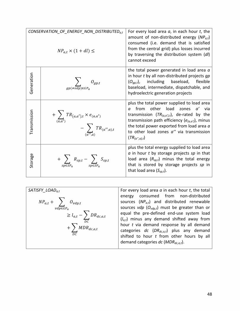
48

CONSERVATION_OF_ENERGY_NON_DISTRIBUTEDa,t

For every load area a, in each hour t, the amount of non-distributed energy (NPa,t) consumed (i.e. demand that is satisfied from the central grid) plus losses incurred by traversing the distribution system (dl) cannot exceed

Gen

erat

ion

∑

the total power generated in load area a in hour t by all non-distributed projects gp (Ogp,t), including baseload, flexible baseload, intermediate, dispatchable, and hydroelectric generation projects

Tran

smis

sio

n

∑ ( )

∑

plus the total power supplied to load area a from other load zones a’ via transmission (TR(a,a’),t), de-rated by the transmission path efficiency (e(a,a’)), minus the total power exported from load area a to other load zones a’’ via transmission (TR(a’’,a),t)

Sto

rage

∑

∑

plus the total energy supplied to load area a in hour t by storage projects sp in that load area (Rsp,t) minus the total energy that is stored by storage projects sp in that load area (Ssp,t).

SATISFY_LOADa,t

∑

∑

∑

For every load area a in each hour t, the total energy consumed from non-distributed sources (NPa,t) and distributed renewable sources vdp (Ovdp,t) must be greater than or equal the pre-defined end-use system load (la,t) minus any demand shifted away from hour t via demand response by all demand categories dc (DRdc,a,t) plus any demand shifted to hour t from other hours by all demand categories dc (MDRdc,a,t).

49

3.6.2 RESERVE MARGIN CONSTRAINTS

1. The capacity reserve constraints address the system risk that arises from power plants outages due to various mechanical and electrical failures. The capacity reserve constraints require that be power system maintain capacity reserve each load area in all hours, i.e. that there would have sufficient capacity available to provide at least 15 percent extra power above demand in every load area in every hour if all generators were working properly. In calculating the capacity reserve margin, the output of generators are therefore not de-rated by forced outage rates. Outages from the failure of transmission or storage assets are included via the use of the dispatch variables (TR, R, S), which have already been de-rated by forced outage rate. SWITCH determines the reserve margin schedule concurrently with the load-satisfying dispatch schedule.

CONSERVATION_OF_ENERGY_NON_DISTRIBUTED_RESERVEa,t

In every load area a, in each hour t, the amount of non-distributed capacity available to meet the capacity reserve margin (NPRa,t) plus losses incurred by traversing the distribution system (dl) cannot exceed

Gen

erat

ion

Cap

acit

y

∑(∑

)

∑ (∑

)

∑ (∑ ( )

)

the total capacity of all variable renewable non-distributed projects (Gvcp,i) multiplied by their capacity factor in hour t (cfvcp,t), plus the total capacity of all dispatchable (dp), intermediate (ip), and hydro (hp) projects (Gp,i) plus the total capacity (Gp,i), adjusted by scheduled outage rate (sp), of all flexible baseload (fbp) and baseload projects (bp) in load area a in hour t

Tran

smis

sio

n

Cap

acit

y

∑

∑

plus the total power transmitted to load area a from other load zones a’ (TR(a,a’),t), de-rated for the path’s transmission efficiency (e(a,a’)), minus the total power transmitted from load area a to other load zones a’’ (TR(a’’,a),t)

50

Sto

rage

C

apac

ity

∑

∑

plus the total output, of storage projects sp in load area a in hour t (Rsp,t) minus the energy stored by storage projects sp (Ssp,t).

SATISFY_RESERVE_MARGINa,t

∑

( ∑

∑

)

For each load area a, in each hour t, the total non-distributed capacity (NPRa,t) and variable renewable distributed output within that load area (Ovdp,t) available for consumption must be a pre-specified reserve margin (r) above the pre-defined system load (la,t) minus any demand shifted away from hour t via demand response by all demand categories dc (DRdc,a,t) plus any demand shifted to hour t from other hours by all demand categories dc (MDRdc,a,t). r is usually set at 0.15 for all load zones in all investment periods.

2. The operating reserve constraints ensure that electricity supply is able to follow electricity

demand on the sub-hourly timescale. Operating reserve (spinning and quickstart) equal to a percentage of demand plus a percentage of variable renewable generation is maintained in each balancing area in each hour. At least half of the operating reserves must be spinning. Frequency or inertial reserves are not modeled.

SATISFY_SPINNING_RESERVEba,t

∑

∑

In each balancing area ba in each hour t, the spinning reserve (SRp,t) provided by dispatchable (DPba) and intermediate plants (IPba), plus the operating reserve (OPp,t) provided by storage plants (SPba) and hydroelectric plants (Hba) must equal or exceed the spinning reserve requirement (spinning_reserve_reqtba,t) in that balancing area in that hour. The spinning reserve requirement is calculated as a percentage of demand plus a percentage of variable renewable generation in each balancing area in each hour.

SATISFY_OPERATING_RESERVEba,t In each balancing area ba in each hour t, the spinning reserve (SRp,t) plus the quickstart reserve, (Qp,t) provided by dispatchable (DPba) and intermediate plants (IPba) plus the operating

51

∑

∑

reserve (OPp,t) provided by storage plants (SPba) and hydroelectric plants (Hba) must equal or exceed the total operating (spinning plus quickstart) reserve requirement (operating_reserve_reqtba,t) in that balancing area in that hour. The operating reserve requirement is calculated as a percentage of demand plus a percentage of renewable generation in each balancing area in each hour.

3.6.3 POLICY CONSTRAINTS

1. The carbon cap constraint requires that the total carbon dioxide emissions from all generation sources cannot exceed a pre-specified emissions cap in every investment period. Emissions are incurred for power generation, provision of spinning reserves, cycling of plants below full load, and generator start-up. As implemented here, the carbon cap constraint limits the total amount of carbon emissions across all of WECC in each study period to a pre-defined level, generally reaching roughly 85 percent reductions relative to 1990 carbon emissions levels for the investment period 2046-2055. The reference 1990 carbon emissions from electricity generation is 284.8 MtCO2/yr. Non-CO2 greenhouse gas emissions from power generation are not included. An iterative process between the investment optimization and the post-investment dispatch check ensures that the final emissions quoted are those that would be incurred when operating the power system over an entire year of hourly data, rather than just the hours sampled in the investment optimization.

CARBON_CAPi

∑

∑

∑

In every period i, the total carbon emissions cannot exceed a pre-specified carbon cap (carbon_capi) for that period. Emissions are incurred from power generation (calculated as the project output (Op,t) times the project heat rate at full load (hrp) times the CO2 content of the fuel for that project (

)); plus the

carbon emissions from spinning reserve from dispatchable and intermediate projects (calculated as the amount of spinning reserves provided (SRp,t) times the project per unit heat rate penalty for providing spinning reserve (sr_penaltyp) times the CO2 content of the fuel for that project (

)); plus the carbon

emissions from deep-cycling flexible baseload and intermediate projects below full load

52

∑

(calculated as the amount below full load (DCp,t) times the heat rate penalty for cycling below full load (dc_penaltyp) times the CO2 content of the fuel for that project (

));

plus the emissions from starting up intermediate and dispatchable plants (calculated as the capacity started up since the previous hour (STp,t) times the startup fuel required (startup_fuelp) times the CO2 content of the fuel for that project (

)). All hourly

values are weighted by the hours represented by each sampled hour t (hst).

2. The RPS constraints require that a certain percentage of end-use demand be met by

renewable energy sources in each load-serving entity, consistent with state-based Renewable Portfolio Standards. A load-serving entity may encompass a single load area or many load zones. More specifically, in each load-serving entity and in each investment period, the ratio of renewable energy certificates (RECs) delivered to that load-serving entity by qualifying renewable sources to end-use demand is greater than or equal to the fraction of end-use demand specified by existing RPS targets. Existing RPS targets are broken into two different categories: primary and distributed. Primary RPS targets can be satisfied by either distributed or central station renewable generation sources, whereas distributed RPS targets can only be satisfied by distributed renewable generation sources. The RPS constraints do not allow the use of unbundled (tradable) RECs, but primary RPS targets may be met by power imported over reserved transmission capacity as controlled by the CONSERVATION_OF_REC constraint. By definition, RECs do not undergo transmission, storage or distribution losses.

MEET_PRIMARY_RPSlse,i

∑

∑

For every load-serving entity lse in every investment period i, the proportion of the renewable energy certificates consumed (REClse,t) in all load zones a within that load-serving entity (the set Alse) in all hours t of that period (the set Ti) as a fraction of total end-use demand (la,t) in that period in that load-serving entity must be greater than or equal to the pre-defined primary RPS fraction (rps_plse,i), for that load-serving entity for that period. Each timepoint in the set Ti is weighted by the number of sample hours it represents (hst).

53

CONSERVATION_OF_REClse,t

∑

∑

∑

For every load-serving entity lse in every hour t, the amount of renewable energy consumed (REClse,t) cannot exceed the total output of renewable generators (Orp,t) in the load-serving entity in that hour plus the energy from RPS-eligible fuels (fR)

transmitted into the load-serving entity (TR(a,a’),f,t) minus the energy from RPS-eligible fuels transmitted out of the load-serving entity (TR(a’’,a),f,t). Only transmission between load zones within different load-serving entities is included in the sums above. By definition, RECs do not undergo transmission, storage or distribution losses.

MEET_DISTRIBUTED_RPSlse,i

∑

∑

For every load-serving entity lse in every investment period i, the proportion of the power generated (Ovdp,t) from distributed renewable sources vdp in that load-serving entity (VDPlse) in all hours t of that period (the set Ti) as a fraction of total load (la,t) in that period in that load-serving entity must be greater than or equal to the pre-defined distributed RPS fraction (rps_dlse,i), for that load-serving entity for that period. Each timepoint in the set Ti is weighted by the number of sample hours it represents (hst).

3. The California Solar Initiative constraint requires the installed capacity of distributed solar projects in California to meet or exceed 3 GW by 2016 and to maintain this capacity in all subsequent investment periods. This constraint can be met with either commercial or residential photovoltaics.

CALIFORNIA_SOLAR_INITIATIVEi≥2016

∑

For every investment period i that occurs on or after the year 2016, the sum of installed capacity of variable renewable distributed projects (Gvdp,i) within the state of California must exceed a pre-specified target capacity (csi_target). csi_target is taken as 3,000 MW. The operational generator lifetime limits the extent of the sum over i to only periods in which the generator would still be operational, but is not included here for simplicity.

54

4. The California Distributed Generation Mandate constraint, not enabled by default, requires the installed capacity of distributed solar projects in California to meet or exceed 12 GW by 2020 and to maintain this capacity in all subsequent investment periods. This constraint can be met with either commercial or residential photovoltaics. This constraint is only included in scenarios that explicitly include the California distributed generation mandate.

CALIFORNIA_DG_MANDATEi≥2020

∑

For every investment period i that occurs on or after the year 2020, the sum of installed capacity of variable renewable distributed projects (Gvdp,i for projects in VDPcal) within the state of California must exceed a pre-specified target capacity (ca_dg_target). ca_dg_target is taken as 12,000 MW. The operational generator lifetime limits the extent of the sum over i to only periods in which the generator would still be operational, but is not included here for simplicity.

5. The Mexico net export constraint caps the growth rate of net power exports from Mexico to surrounding load zones in the United States at no more than the historical electric power export growth rate between 2003 and 2008 of 3.2%/yr (Secretaría de Energía 2010). Baja California Norte is the only Mexican load area simulated. This constraint does not represent a specific public policy, but instead ensures that Mexico can export power to United States load zones while restricting the growth of exports to realistic levels.

3.6.4 RESOURCE CONSTRAINTS

Large energy projects tend to be limited in size due to resources constraints such as land availability, geology, resource quality, etc. All renewable resources in SWITCH are constrained by resource availability. In addition, the availability of cogeneration with either renewable or non-renewable fuels is constrained to present levels. Compressed air energy storage is resource-constrained by underground geology. Other non-renewable resources (non-cogeneration natural gas, oil, coal, and nuclear) do not have explicit resource constraints, but

∑

∑

MEX_EXPORT_LIMITa=MEX_BAJA,i

For each investment period i, the sum of transmission capacity dispatched out of the load area a=MEX_BAJA, (TR(a,a’),t) minus the sum of transmission capacity dispatched into the load area a=MEX_BAJA (TR(a’’,a),t), weighted by the number of sample hours represented by hour t (hst), cannot exceed the specified export limit out of MEX_BAJA (mex_export_limi).

55

are instead limited by cost and/or policy measures and are therefore not discussed further in this section.

1. For capacity limited projects (residential and commercial photovoltaic, geothermal, offshore and onshore wind, and compressed air energy storage), the amount of installed capacity at a specific project cannot exceed a pre-specified MW capacity limit.

MAX_RESOURCE_PROJECTclp,i

∑

For each capacity-limited project clp in every investment period i, the sum of generation capacity installed at the project in the current and all preceding periods i (Gclp,i) must not exceed the pre-specified capacity limit for that project (clclp). The operational generator lifetime limits the extent of the sum over i to only periods in which the generator would still be operational, but is not included here for simplicity.

2. Central station solar projects compete for the same locations and are thus constrained to not exceed the pre-specified available land area of any specific piece of land. Central station solar projects include central station photovoltaics and solar thermal trough systems with and without thermal storage.

MAX_RESOURCE_LANDloc,i

∑

For each location loc in which land-area-limited projects are sited and every investment period i, the total capacity of land-area-limited projects llp at that location installed in the current and all preceding periods i (Gllp,i), divided by the land area per unit of installed capacity for the project (lallp) must not exceed the pre-specified land-area limit for that location (llloc). The generator operational lifetime limits the extent of the sum over i to only periods in which the generator would still be operational, but is not included here for simplicity.

3. Biogas and biomass solid projects are limited by the pre-specified amount of biogas or biomass available within each load area in each investment period.

MAX_RESOURCE_BIObf,a,i

For each biofuel (biomass solid and biogas) bf in every load area a in every investment period i, the total consumption of that biofuel must not exceed a pre-specified biofuel availability limit

56

∑

(bflbf,a,i). The total consumption of biofuel is calculated as the sum over all bio-limited projects blp of biofuel type bf in all hours t in investment period i of power produced by bio-limited projects (Oblp,bf,t), multiplied by the project’s heat rate (hrblp) plus cogeneration thermal demand (in units of thermal energy demanded per MW generated) (ctdblp), weighted by the number of hours represented by hour t (hst). The cogeneration heat demand term is zero for non-cogen plants. The operational generator lifetime limits the extent of the sum over i to only periods in which the generator would still be operational, but is not included here for simplicity.

4. The amount of cogeneration resource available is limited by the current installed capacity at each cogeneration plant.

MAX_RESOURCE_COGENcbp,i

∑

For each cogeneration project cbp in every investment period i, the sum of generation capacity installed at the project in the current and all preceding periods i (Gcbp,i) must not exceed the pre-specified capacity limit for that project (clcbp). The operational generator lifetime limits the extent of the sum over i to only periods in which the generator would still be operational, but is not included here for simplicity.

3.6.5 TRANSMISSION AND DISTRIBUTION CONSTRAINTS

1. Transmission paths can transfer no more energy in each hour in each direction between each pair of connected load zones than the path’s rated thermal capacity, de-rated by its path de-rating factor. Once transmission capacity is installed, it is assumed to remain in operation for the remainder of the study.

MAX_TRANS(a,a’),t

For each transmission path (a, a’) in every hour t, the total amount of energy dispatched along the transmission path between two load zones (a,a’) in each hour t (TR(a,a’),t) cannot exceed the sum of the pre-existing thermal transmission capacity (et(a,a’)) and the sum of additional thermal

57

∑

transmission capacity installed between the two load zones in the current and all preceding periods i (T(a,a’),i), de-rated by the transmission path’s de-rating factor (path_derate(a,a’)).

2. Distribution capacity must be installed in order to serve peak demand in each load area and

in each investment period. If demand response is not enabled, then only the MIN_DISTRIBUTION_NO_DR is enforced and consequently the amount of distribution capacity installed is completely determined by the exogenously specified demand profile. If demand response is enabled, both the MIN_DISTRIBUTION_DR and MIN_DISTRIBUTION_NO_DR constraints are enforced. Consequently, additional distribution capacity above projected peak demand may be installed in order to allow for demand response to shift demand to hours of peak demand. Such an event may occur if variable renewable generation exhibits a positive correlation with hours of peak demand.

MIN_DISTRIBUTION_NO_DRa,i

∑

For each load area a in every investment period i, the pre-defined maximum end-use system load in period i (mla,i) must be less than or equal to the sum of pre-existing distribution capacity (eda) and additional distribution capacity installed in the load area in the current and all preceding periods i (Da,i).

MIN_DISTRIBUTION_DRa,t

∑

∑

∑

For each load area a in every hour t, the pre-defined end-use system load (la,t), minus any demand response provided in hour t from all demand categories dc (DRdc,a,t) plus any demand shifted to hour t from other hours from all demand categories dc (MDRdc,a,t), must be less than or equal to the sum of the pre-existing distribution capacity (eda) and additional distribution capacity installed in the load area in the current and all preceding periods i (Da,i). This constraint is written over the set of hours t but will only be binding for a small number of hours in each investment period (likely only one), thereby setting the amount of distribution capacity installed in the investment period.

58

3.6.6 OPERATIONAL CONSTRAINTS

1. Variable renewable generators (solar and wind) produce the amount of power corresponding to their simulated historical power output in each hour, de-rated by their forced outage rate.

VAR_GENvp,t

∑

For each variable renewable generation project vp in every hour t, the expected amount of power produced by the variable renewable generator in that hour (Ovp,t) must equal the sum of generator capacity installed at generator vp in the current and preceding investment periods i (Gvp,i), de-rated by the generator’s forced outage rate (ovp), multiplied by the generator’s capacity factor in hour t (cfvp,t). The operational generator lifetime limits the extent of the sum over i to only periods in which the generator would still be operational, but is not included here for simplicity.

2. Baseload generators (nuclear, geothermal, biomass solid, biogas and cogeneration) must produce an amount of power equal to their installed nameplate capacity, de-rated by their forced and scheduled outage rates, in all hours in each investment period.

BASELOAD_GENbp,t

∑

For every baseload project bp and every hour t, the expected amount of power produced by the baseload generator in that hour (Obp,t) cannot exceed the sum of generator capacity installed at generator bp in the current and preceding investment periods i (Gbp,i), de-rated by the generator’s forced outage rate (obp) and scheduled outage rate (sbp). The operational generator lifetime limits the extent of the sum over i to only periods in which the generator would still be operational, but is not included here for simplicity.

3. Flexible baseload generators (non-cogeneration coal) cannot commit more capacity in each

day than their nameplate capacity, de-rated by their forced and scheduled outage rates.

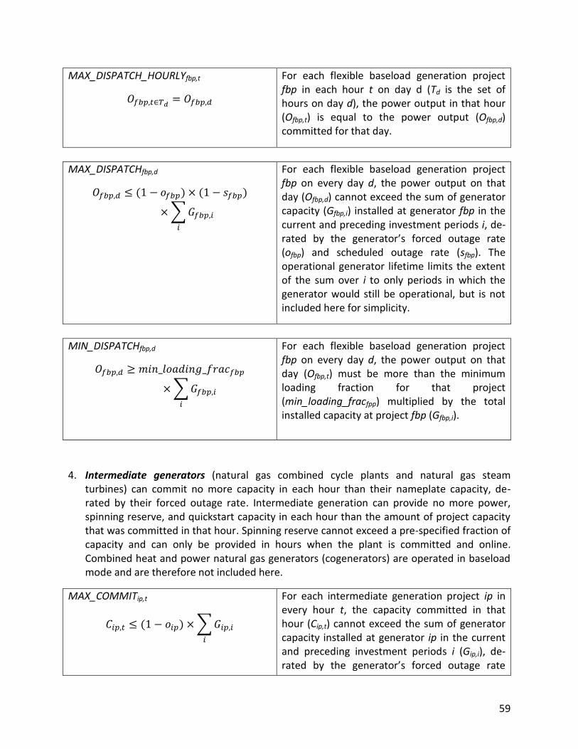
59

MAX_DISPATCH_HOURLYfbp,t

For each flexible baseload generation project fbp in each hour t on day d (Td is the set of hours on day d), the power output in that hour (Ofbp,t) is equal to the power output (Ofbp,d) committed for that day.

MAX_DISPATCHfbp,d

∑

For each flexible baseload generation project fbp on every day d, the power output on that day (Ofbp,d) cannot exceed the sum of generator capacity (Gfbp,i) installed at generator fbp in the current and preceding investment periods i, de-rated by the generator’s forced outage rate (ofbp) and scheduled outage rate (sfbp). The operational generator lifetime limits the extent of the sum over i to only periods in which the generator would still be operational, but is not included here for simplicity.

MIN_DISPATCHfbp,d

∑

For each flexible baseload generation project fbp on every day d, the power output on that day (Ofbp,t) must be more than the minimum loading fraction for that project (min_loading_fracfpp) multiplied by the total installed capacity at project fbp (Gfbp,i).

4. Intermediate generators (natural gas combined cycle plants and natural gas steam

turbines) can commit no more capacity in each hour than their nameplate capacity, de-rated by their forced outage rate. Intermediate generation can provide no more power, spinning reserve, and quickstart capacity in each hour than the amount of project capacity that was committed in that hour. Spinning reserve cannot exceed a pre-specified fraction of capacity and can only be provided in hours when the plant is committed and online. Combined heat and power natural gas generators (cogenerators) are operated in baseload mode and are therefore not included here.

MAX_COMMITip,t

∑

For each intermediate generation project ip in every hour t, the capacity committed in that hour (Cip,t) cannot exceed the sum of generator capacity installed at generator ip in the current and preceding investment periods i (Gip,i), de-rated by the generator’s forced outage rate

60

(oip). The operational generator lifetime limits the extent of the sum over i to only periods in which the generator would still be operational, but is not included here for simplicity.

MIN_DISPATCHip,t

For each intermediate generation project ip in every hour t, the power output in that hour (Oip,t) must be more than the minimum loading fraction for that project (min_loading_fracip) multiplied by total committed capacity in that hour (Cip,t).

MAX_DISPATCHip,t

For each intermediate generation project ip in every hour t, the expected amount of power (Oip,t), spinning reserve (SRip,t), and quickstart capacity (Qip,t) supplied by the intermediate generator in that hour cannot exceed the generator capacity committed in that hour (Cip,t).

MAX_SPINip,t

For each intermediate generation project ip in every hour t, the spinning reserve supplied by the project in that hour (SRip,t) cannot exceed a pre-specified fraction of committed capacity (spin_fracip). This constraint is tied to the amount of capacity actually committed (Cip,t) to ensure that spinning reserve is only provided in hours when the plant is also producing useful generation. The parameter spin_fracip is calculated using the generator’s 10-minute ramp rate.

STARTUPip,t

For each intermediate project ip in every hour t, the amount of capacity started up (STip,t) equals the committed capacity in hour t (Cip,t) minus the committed capacity in the previous simulated hour (Cip,t-1). Hours within each study day are defined circularly (the first hour of the day is preceded by the last hour of the same day) for the purpose of generator startup. STip,t should be considered a derived variable as this constraint will be binding due to startup

61

costs incurred when Cip,t and Cip,t-1 are not equal.

5. Dispatchable generators (natural gas combustion turbines) can provide no more power, spinning reserve, and quickstart capacity in each hour than their nameplate capacity, de-rated by their forced outage rate. Spinning reserve can only be provided in hours when the plant is also producing useful generation and cannot exceed a pre-specified fraction of capacity.

MAX_DISPATCHdp,t

∑

For each dispatchable generation project dp in every hour t, the expected amount of power (Odp,t), spinning reserve (SRdp,t), and quickstart capacity (Qdp,t) supplied by the project in that hour cannot exceed the sum of capacity installed at the project dp in the current and preceding periods i (Gdp,i), de-rated by the generator’s forced outage rate (odp). The generator’s operational lifetime limits the extent of the sum over i to only periods in which the generator would still be operational, but is not included here for simplicity.

MAX_SPINdp,t

For each dispatchable project dp in every hour t, the spinning reserve supplied by the dispatchable generator in that hour (SRdp,t) cannot exceed a pre-specified fraction (spin_fracdp) of power dispatched by the dispatchable project (Odp,t). This constraint ties the dispatch of spinning reserve to the amount of power actually dispatched Odp,t to ensure that spinning reserve is only provided in hours when the plant is also producing power.

STARTUPdp,t

For each dispatchable project dp in every hour t, the amount of capacity started up (STdp,t) equals the power output in hour t (Odp,t) minus the power output in the previous simulated hour (Odp,t-1). Hours within each study day are defined circularly (the first hour of the day is preceded by the last hour of the same day) for the purpose of generator startup. STdp,t should be considered a derived

62

variable as this constraint will be binding due to startup costs incurred when Odp,t and Odp,t-1 are not equal.

6. Hydroelectric generators must provide output in each hour equal to or exceeding a pre-specified fraction – usually 50% – of the average hydroelectric capacity factor for the month in which the study day resides in order to maintain downstream water flow. The total energy (which, for pumped hydro, includes energy released from storage) and operating reserves provided by each hydro project in each hour cannot exceed the project’s total turbine capacity, de-rated by the forced outage rate of hydroelectric generators. Operating reserves from hydro cannot exceed a pre-specified fraction of installed capacity – usually 20%. The capacity factor for all hydroelectric facilities in a load area over the course of each study day must equal the historical daily average capacity factor for the month in which that day resides. New hydroelectric facilities are not built, but existing facilities are operated indefinitely. The dispatch of hydroelectric projects is aggregated to the load area level to reduce the number of decision variables. All load area level hydro dispatch decisions are allocated to individual projects on an installed capacity basis.

HYDRO_MIN_DISPhp,t

For every hydroelectric project hp in every hour t on day d (Td is the set of hours on day d), the amount of energy in dispatched by the project (Ohp,t) must be greater than or equal to a pre-specified average capacity factor for that project for that day (cfhp,d), multiplied by the project’s installed capacity (hghp), multiplied by a pre-specified minimum dispatch fraction (min_dispatch_frac), necessary to maintain stream flow.

HYDRO_MAX_DISPhp,t

For every hydroelectric project hp in every hour t, the sum of watershed energy output (Ohp,t) and operating reserve (OPhp,t) as well as, for pumped hydroelectric projects php, energy dispatched from storage (Rphp,t), and operating reserve from storage (OPphp), cannot exceed the project’s installed capacity (hghp) de-rated by the project’s forced outage rate (ohp).

63

HYDRO_MAX_OP_RESERVEhp,t

For every hydroelectric project hp in every hour t, the amount of operating reserve dispatched (OPhp,t) cannot exceed a fraction (hydro_op_reserve_frac) of the project’s installed capacity (hghp).

HYDRO_AVG_OUTPUThp,d

∑

For every hydroelectric project hp and every day d, the historical average energy output must be met, i.e. the sum over all hours t on day d of energy dispatched by the hydroelectric project (Ohp,t) plus the fraction of time operating reserves are deployed (op_reserve_deploy_frac) multiplied by the operating reserve provided by the hydroelectric project (OPhp,t) must equal the historical average capacity factor of the hydroelectric project (cfhp,d) on day d multiplied by the project’s installed capacity (hghp) multiplied by the number of hours simulated in day d (num_hours_simulatedd). Td is the set of hours on day d.

7. Storage facilities (battery storage, pumped hydroelectric, and compressed air energy

storage (CAES)) can store no more power in each hour than their maximum hourly store rate, de-rated by a forced outage rate, and dispatch no more power in each hour than total capacity, de-rated by a forced outage rate. CAES projects must maintain the proper ratio between dispatch of energy stored in the form of compressed air and energy dispatched from natural gas. In SWITCH, days are modeled as independent dispatch units, and as such, the energy dispatched by each storage project on each day must equal the energy stored by the project on that day, adjusted for the storage project’s round-trip efficiency losses.

MAX_STORE_RATEsp,t

∑

For every storage project sp in every hour t, the amount of energy stored (Ssp,t) cannot exceed the product of a pre-specified store rate for that project (rsp) and the total capacity installed at that project in the current and preceding periods i (Gsp,i), de-rated by the storage project’s forced outage rate (osp). For pumped hydro, Gsp,t is equal to the preexisting capacity as no new capacity can be installed. The storage project operational lifetime limits the extent of the sum over i to only periods in which the storage project would still be operational, but is not

64

included here for simplicity.

MAX_BATTERY_STORAGE_DISPATCHbp,t

∑

For every battery storage project bp in every hour t, the amount of energy dispatched from the storage project in that hour (Rbp,t) plus the operating reserve provided in that hour (OPbp,t) cannot exceed the sum of the storage project’s power capacity installed in the current and preceding periods i (Gbp,i), de-rated by the storage project’s forced outage rate (os). The storage project operational lifetime limits the extent of the sum over i to only periods in which the storage project would still be operational, but is not included here for simplicity.

MAX_CAES_DISPATCHcp,t

∑

For every CAES storage project cp in every hour t, the sum of the energy released from storage (Rcp,t) and operating reserve (OPcp,t) provided by the storage plant plus the energy (Ocp,t), spinning reserve (SRcp,t) and quickstart reserve (Qcp,t) provided from natural gas cannot exceed the plant’s total power capacity installed in the current and preceding periods i (Gcp,i), de-rated by the plant’s forced outage rate (ocp). The storage project operational lifetime limits the extent of the sum over i to only periods in which the storage project would still be operational, but is not included here for simplicity.

CAES_COMBINED_DISPATCHcp,t

For every CAES project cp in every hour t, the amount of energy dispatched from storage (Rcp,t) must equal the amount of energy dispatched from natural gas (Ocp,t) multiplied by the dispatch ratio between storage and natural gas (caes_ratio). caes_ratio is derived from the storage efficiency and overall round-trip efficiency of CAES and is calculated to be 1.40.

65

CAES_COMBINED_ORcp,t

For every CAES project cp in every hour t, the amount of operating reserve dispatched from the CAES project in that hour (ORcp,t) must equal the operating reserve (spinning plus quickstart) dispatched from natural gas (SRcp,t + Qcp,t) multiplied by the dispatch ratio between storage and natural gas (caes_ratio).

STORAGE_ENERGY_BALANCEsp,d

∑

∑

∑

For each storage project sp on each day d, the energy dispatched by the storage project in all hours t on day d (Rsp,t) must equal the energy stored by the storage project in all hours t on day d, de-rated by the storage project’s round-trip efficiency (esp). It is assumed that operating reserve (ORsp,t) is called upon a fraction of the time, (op_reserve_deploy_frac), and is therefore included in the energy balance. Td is the set of hours on day d.

3.6.7 DEMAND RESPONSE CONSTRAINTS

By default demand response is disabled. When demand response is enabled, the amount of demand that can be moved from or to an hour via demand response for each demand category in each load area is limited to a pre-specified amount of energy. Over the course of a day, the total demand moved from and to all hours must sum to zero for each demand category in each load area – the total amount of demand met over the course of a day is the same with or without demand response. The two demand categories that can participate in demand response are electric vehicles and buildings (residential + commercial). The amount of demand that can be moved from or to an hour from electric vehicles is calculated using battery charging rates (Section 2.5: Demand Response Hourly Potentials).

MAX_DR_FROMdc,a,t

For every demand category dc in every load area a in every hour t, the amount of demand moved from an hour via demand response (DRdc,a,t) must be less than or equal to a pre-specified energy limit (dr_from_limitdc,a,t).

66

MAX_DR_TOdc,a,t

For every demand category dc in every load area a in every hour t, the amount of demand moved to an hour via demand response (MDRdc,a,t) must be less than or equal to a pre-specified energy limit (dr_to_limitdc,a,t).

DR_ENERGY_BALANCEdc,a,d

∑

∑

For every demand category dc in every load area a in every day d, the amount of demand moved from all hours t on day d (Td is the set of hours on day d) via demand response (DRdc,a,t) must be equal to the amount of demand moved to all hours t on day d via demand response (MDRdc,a,t).

67

3.7 PRESENT-DAY DISPATCH

For the purpose of having a benchmark to which to compare future investment plans, we perform a present-day optimization for each scenario. In this present-day optimization, all current generation, transmission, and storage capacity is operated subject to the constraints described above, but no new capacity is built with the exception of natural gas combustion turbines. The simulation year is fixed as 2013 (the year in which this study was performed), and parameters such as demand projections, fuel prices, biomass availability, etc., that vary by year are taken from 2013. Policy targets such as renewable portfolio standards, carbon caps, and distributed generation targets are not enforced as the data sources on which existing power system asset capacity is based tends to lag behind that which is in the ground by a few years. The exclusion of policy constraints makes present-day dispatch an imperfect benchmark, but present-day dispatch still includes many important current aspects of power system economics and therefore is an acceptable benchmark for purposes of comparison to future investment results.

3.8 POST-INVESTMENT DISPATCH CHECK

The decisions made by each SWITCH optimization use a limited number of sampled hours over which to dispatch the electric power system. While the model has state-of-the art hourly resolution for a large-scale capacity expansion model, each investment period optimizes on 144 sampled hours – much less than a full year of load and intermittent renewable data. To verify that the model has in fact designed a power system that can function over a full year of hourly load and intermittent renewable output data, a post-investment dispatch check is included. In this check, performed after each investment optimization, all investment decisions are held fixed and new, unseen hourly data are tested in batches of one day at a time. If there is not sufficient generation capacity to meet demand, operational, and reserve constraints on a given day, more peaking gas combustion turbine capacity is added to the system to compensate.

In total, 364 distinct days (8736 distinct hours) are simulated in the post-investment dispatch check. One day per year is not simulated because time zone conversion results in incomplete data for that day. The hourly weighting scheme used in the post-investment dispatch check ensures that 365 days per year are represented, so we refer to the simulated 8736 hours as a year of hourly data.

In addition to investment decision variables, three sets of prices in each investment period are determined by the investment optimization and subsequently passed to the post-optimization dispatch check:

1. Carbon price – taken from the dual value of the carbon cap constraint for each investment period. The carbon price has a uniform value over the entire WECC for each period in the post-dispatch optimization.

2. Natural gas fuel price – calculated as the sum of all expenditures on natural gas in a period divided by the quantity of natural gas consumed in that period. The natural gas

68

price has a uniform value over the entire WECC for each period in the post-dispatch optimization.

3. Biomass solid fuel price – calculated as the sum of all expenditures on biomass solid fuel in a load area in a period divided by the quantity of biomass solid fuel consumed in that period in that load area. The biomass solid fuel price has a uniform value over each load area for each period in the post-investment dispatch check.

The current version of the post-investment dispatch check does not enforce the capacity reserve margin constraint, though the capabilities of grid assets are de-rated by forced and scheduled outage rates as is the case in the investment optimization. The dispatch check uses the same constraints and general structure as the investment optimization and therefore does not include binary unit commitment constraints, security constraints, or load flow transmission constraints.

Annual RPS targets and carbon emission caps are not included in the post-optimization dispatch check in order to allow the problem to be decomposed into separate optimization problems for each day. Unlike the main optimization, the dispatch simulation does not track renewable electricity through the transmission network and consequently does not report whether RPS targets can be met with the larger number of time points. Results from the investment optimization tend to be in most cases quantitatively similar to results from the post-investment dispatch check, so the omission of RPS targets in the post-investment dispatch check is not thought to introduce substantial error. When reporting the amount of imported or exported power to or from California of either renewable or non-renewable variety, it is assumed that the fraction of renewable and non-renewable power dispatched across the California border is equivalent in the investment optimization and the post-optimization dispatch check.

The post-investment dispatch check includes a price on carbon emissions in order to emulate the behavior of the carbon cap in the investment optimization. The carbon price is not guaranteed to produce identical emissions between the two problems, and as such an emissions true-up is performed.

69

4 REFERENCES

3TIER, 2010. Development of regional wind resource and wind plant output datasets. National Renewable Energy Laboratory, Subcontract Report NREL/SR-550-47676, March 2010.

American Wind Energy Association, 2010. U.S. wind energy projects. Washington, DC, 2010; http://www.awea.org/projects/). Black and Veatch, 2012a. Capital costs for transmission and substations: recommendations for WECC transmission expansion planning. B&V project no. 176322; http://www.wecc.biz/committees/BOD/TEPPC/External/BV_WECC_TransCostReport_Final.pdf. Black and Veatch, 2012b. Cost and performance data for power generation technologies. Overland Park, KS, 2012; http://bv.com/docs/reports-studies/nrel-cost-report.pdf. California Air Resources Board, 2013. AB32 Scoping Plan Website; www.arb.ca.gov/cc/scopingplan/scopingplan.htm.

California Council on Science and Technology, 2011. California’s energy future – the view to 2050; http://www.ccst.us/publications/2011/2011energy.php.

California Energy Commission, 2010. Cost of generation model, version 2; http://www.energy.ca.gov/2010publications/CEC-200-2010-002/index.html. California Environmental Protection Agency, 2011. Statewide water quality control policy on the use of coastal and estuarine waters for power plant cooling, State Water Resources Control Board; http://www.waterboards.ca.gov/water_issues/programs/ocean/cwa316/docs/otc_clean.pdf. California Public Utilities Commission, 2013. About the California Solar Initiative; http://www.cpuc.ca.gov/PUC/energy/Solar/aboutsolar.htm Canadian Wind Energy Association, 2012. List of wind farms; http://www.canwea.ca/farms/wind-farms_e.php. Chaudhari, M., L. Frantzis, T. E. Hoff, 2004. PV grid connected market potential under a cost breakthrough scenario. Navigant Consulting, Burlington, Massachusetts, 2004; http://www.ef.org/documents/EF-Final-Final2.pdf. Margolis, R., Coggeshall, C., and Zuboy, J., 2012. SunShot Vision Study. US Department of Energy.

Denholm, P. and R. Margolis, 2007. Supply curves for rooftop solar PV-generated electricity for the United States. National Renewable Energy Laboratory, Boulder, CO, Technical Report NREL/TP-6A0-44073, 2007; http://www.nrel.gov/docs/fy09osti/44073.pdf.

http://www.awea.org/projects/

http://www.wecc.biz/committees/BOD/TEPPC/External/BV_WECC_TransCostReport_Final.pdf

http://bv.com/docs/reports-studies/nrel-cost-report.pdf

http://www.arb.ca.gov/cc/scopingplan/scopingplan.htm

http://www.ccst.us/publications/2011/2011energy.php

http://www.energy.ca.gov/2010publications/CEC-200-2010-002/index.html

http://www.waterboards.ca.gov/water_issues/programs/ocean/cwa316/docs/otc_clean.pdf

http://www.cpuc.ca.gov/PUC/energy/Solar/aboutsolar.htm

http://www.canwea.ca/farms/wind-farms_e.php

http://www.ef.org/documents/EF-Final-Final2.pdf

http://www.nrel.gov/docs/fy09osti/44073.pdf

70

de la Torre Ugarte, D. and D.E. Ray, 2000. Applications of the POLYSIS Modeling Framework. Biomass and Bioenergy 18(4) p. 291-308.

Electric Power Research Institute, 2002. Handbook of Energy Storage for Transmission or Distribution Applications. Technical Update, Palo Alto, CA, December 2002.

Electric Power Research Institute, 2003. Handbook of energy storage for transmission and distribution applications. Palo Alto, CA, 2003.

Electric Power Research Institute, 2010. Electricity energy storage technology options: a white paper primer on applications, costs, and benefits. Technical Update, 1029676.

Electricity Storage Association, 2010. Technologies: pumped hydro. Washington, DC, 2010; http://www.electricitystorage.org/site/technologies/pumped_hydro/. Federal Energy Regulatory Commission, 2006. Form 714: annual electric balancing authority area and planning area report. Washington, DC, 2006.

Federal Energy Regulatory Commission, 2012. Form 715: annual transmission planning and evaluation report, 2012. Washington, DC, 2009.

Fripp, M., 2008. Optimal Investment in Wind and Solar Power in California, doctoral dissertation, University of California, Berkeley, 2008; http://disexpress.umi.com/dxweb#download?&type=pdf&dpubno=3388273.

Fripp, M., 2012. Switch: a planning tool for power systems with large shares of intermittent renewable energy. Accepted in Environmental Science and Technology, 2012.

GE Energy, 2010. Western wind and solar integration study. National Renewable Energy Laboratory, Boulder, CO, Subcontract No. AAM-8-77557-01, 2010; http://www.nrel.gov/wind/systemsintegration/pdfs/2010/wwsis_final_report.pdf). Greenblatt, J. B. et al., 2007. Baseload wind energy: modeling the competition between gas turbines and compressed air energy storage for supplemental generation. Energy Policy 35, 1474-1492 (March 2007).

Klein, J., 2010. Comparative costs of California central station electricity generation technologies: cost of generation model. California Energy Commission, Sacramento, CA, 2007; http://www.energy.ca.gov/2007publications/CEC-200-2007-011/CEC-200-2007-011-SD.PDF. Kumarappan, S. et al., 2009. Biomass supply for biofuel production: estimates for the United States and Canada. BioResources 4(3), 1070-1087. London Economics and Global Energy Decisions, 2007. Performance of six European wholesale electricity markets in 2003, 2004, and 2005, Appendix I;

http://www.electricitystorage.org/site/technologies/pumped_hydro/

http://disexpress.umi.com/dxweb#download?&type=pdf&dpubno=3388273

http://www.nrel.gov/wind/systemsintegration/pdfs/2010/wwsis_final_report.pdf

http://www.sciencedirect.com/science?_ob=PublicationURL&_tockey=%23TOC%235713%232007%23999649996%23639113%23FLA%23&_cdi=5713&_pubType=J&view=c&_auth=y&_acct=C000059607&_version=1&_urlVersion=0&_userid=4420&md5=cb42f0be84c161373b450a7a5c2a1141

http://www.energy.ca.gov/2007publications/CEC-200-2007-011/CEC-200-2007-011-SD.PDF

71

http://ec.europa.eu/competition/sectors/energy/inquiry/electricity_final_appendix1.pdf. Lu, N., et al., 2009. The wide-area energy storage and management system -- battery storage evaluation. Pacific Northwest National Laboratory, July 2009, PNNL-18679.

Mai, T., et al., 2013. Resource Planning Model: an integrated resource planning and dispatch tool for regional electric systems. National Renewable Energy Laboratory, NREL/TP-6A20-56723, January 2013.

Masters, G.M., 2004. Renewable and Efficient Electric Power Systems (Wiley-Interscience, New Jersey, 2004), p. 319.

McGowin, C., 2007. Renewable Energy Technical Assessment Guide. TAG-RE:2007. Palo Alto, CA: Electric Power Research Institute.

Mehos, M. and R. Perez, 2005. Mining for solar resources: U.S. Southwest provides vast potential. Imaging Notes 20 (Summer 2005).

Meinel, A.B. and M.P. Meinel, 1976. Applied Solar Energy (Addison Wesley Publishing Co., Massachusetts, 1976).

Milbrandt, A., 2005. A geographic perspective on the current biomass resource availability in the United States. National Renewable Energy Laboratory, Boulder, CO, 2005.

Mileva, A. et al., 2013. SunShot solar power reduces costs and uncertainty in future low-carbon electricity systems, Environ. Sci. Technol., 2013, in press, DOI: 10.1021/es401898f.

Mills, A., Wiser, R., 2012. An evaluation of solar valuation methods used in utility planning and procurement processes. Ernest Orlando Lawrence Berkeley National Laboratory, LBNL-5933E, December 2012.

National Renewable Energy Laboratory, 2013a. System Advisor Model, v2013.1.15. Boulder, CO; https://sam.nrel.gov/.

National Renewable Energy Laboratory, 2013b. Solar Prospector dataset, Boulder, CO; http://maps.nrel.gov/prospector.

National Energy Technology Laboratory, 2008. National Carbon Sequestration Database and Geographic Information System. United Stated Department of Energy, 2008; http://www.netl.doe.gov/technologies/carbon_seq/natcarb/index.html.

National Oceanic and Atmospheric Administration, 2009. Relative humidity and dewpoint temperature from temperature and wet-bulb temperature. Washington, DC, 2009; http://www.srh.noaa.gov/images/epz/wxcalc/rhTdFromWetBulb.pdf. National Renewable Energy Laboratory, 2013. System Advisor Model. Boulder, Colorado, 2010; https://www.nrel.gov/analysis/sam/).

https://sam.nrel.gov/

http://maps.nrel.gov/prospector

http://www.netl.doe.gov/technologies/carbon_seq/natcarb/index.html

http://www.srh.noaa.gov/images/epz/wxcalc/rhTdFromWetBulb.pdf

https://www.nrel.gov/analysis/sam/

72

North American Electric Reliability Corporation (NERC), 2013. NERC Interconnections map. http://www.nerc.com/AboutNERC/keyplayers/Documents/NERC_Interconnections_Color_072512.jpg Nelson, J. et al., 2012. High-resolution modeling of western North American power system demonstrates low-cost and low-GHG futures. Energy Policy 2012, 43, 436−447.

North American Electric Reliability Corporation, 2007. WECC Standard BAL-STD-002-0 - Operating Reserves; http://www.nerc.com/files/BAL-STD-002-0.pdf. North Carolina State University, 2011. Database of state incentives for renewables and efficiency. Raleigh, NC, 2011; http://www.dsireusa.org/. Hunsaker, M.; Samaan, N.; Guo, T.; Liu, G.; Toolson, J. Balancing authority cooperation concepts to reduce variable generation integration costs in the western interconnection: intra-hour scheduling. Western Electricity Coordinating Council (WECC). 2013; http://energyexemplar.com/wp-content/uploads/publications/Balancing%20Authority%20Cooperation%20Concepts%20-%20Intra-Hour%20Scheduling.pdf

Parker, N. C., 2011. Modeling Future Biofuel Supply Chains using Spatially Explicit Infrastructure Optimization, doctoral dissertation, University of California, Davis, 2011.

Platts Corporation, 2009. POWERmap: Substation Layer. Westminster, CO, 2009; http://www.platts.com/Products/powermap). Secretaría de Energía, 2010. Programa de obras e inversions del sector eléctrico 2010-2024. Mexico, 2010; http://www.energia.gob.mx/portal/Default.aspx?id=1453.

Succar, S. and R. H. Williams, 2008. Compressed air energy storage: theory, resources, and applications for wind power. Princeton Environmental Institute, Princeton, New Jersey, 2008; http://www.princeton.edu/pei/energy/publications/texts/SuccarWilliams_PEI_CAES_2008April8.pdf).

Statistics Canada, 2008. Table 127-0001 - Electric power statistics, monthly (megawatt hour), CANSIM database; http://www5.statcan.gc.ca/cansim/a26?lang=eng&retrLang=eng&id=1270001&paSer=&pattern=&stByVal=1&p1=1&p2=-1&tabMode=dataTable&csid=. Statistics Canada, 2012. Table 127-0002 - Electric power generation, by class of electricity producer, monthly (megawatt hour), CANSIM database; http://www5.statcan.gc.ca/cansim/a26?lang=eng&retrLang=eng&id=1270002&paSer=&pattern=&stByVal=1&p1=1&p2=-1&tabMode=dataTable&csid=.

http://www.nerc.com/AboutNERC/keyplayers/Documents/NERC_Interconnections_Color_072512.jpg

http://www.nerc.com/AboutNERC/keyplayers/Documents/NERC_Interconnections_Color_072512.jpg

http://www.nerc.com/files/BAL-STD-002-0.pdf

http://www.dsireusa.org/

http://energyexemplar.com/wp-content/uploads/publications/Balancing%20Authority%20Cooperation%20Concepts%20-%20Intra-Hour%20Scheduling.pdf



http://www.platts.com/Products/powermap

http://www.energia.gob.mx/portal/Default.aspx?id=1453

http://www.princeton.edu/pei/energy/publications/texts/SuccarWilliams_PEI_CAES_2008April8.pdf

http://www.princeton.edu/pei/energy/publications/texts/SuccarWilliams_PEI_CAES_2008April8.pdf

http://www5.statcan.gc.ca/cansim/a26?lang=eng&retrLang=eng&id=1270001&paSer=&pattern=&stByVal=1&p1=1&p2=-1&tabMode=dataTable&csid




73

The Wind Power, 2010. Wind turbines and wind farms database. Buc, France, 2010; http://www.thewindpower.net/index_turbines.php). University of Tennessee, Agricultural Policy Analysis Center: POLYSYS - Policy analysis System, 2007; http://www.agpolicy.org/polysys.html. United States Department of Defense, 2002. Unified Facilities Criteria (UFC): active solar preheat systems. Washington, DC, UFC 3-440-01, 2002; http://www.wbdg.org/ccb/DOD/UFC/ufc_3_440_01.pdf). United States Department of Energy, 2010. Solar Vision Study. Washington, DC, 2010; http://www1.eere.energy.gov/solar/vision_study.html). United States Department of Labor, 2009. Occupational pay comparisons among metropolitan areas. Bureau of Labor Statistics, Washington, DC, 2009. United States Energy Information Administration, 2007a. Form EIA-860 database annual electric generator report. Washington, DC, 2007. United States Energy Information Administration, 2007b. Form EIA-906. Washington, DC, 2007.

United States Energy Information Administration, 2010a. Annual energy outlook 2010. Washington, DC, 2010. United States Energy Information Administration, 2010b. Updated Capital Cost Estimates for Electricity Generation Plants. Washington, DC, 2010; http://www.eia.gov/oiaf/beck_plantcosts/. United States Energy Information Administration, 2011. Power plant operations report, Form EIA-923. Washington, DC, 2011.

United States Energy Information Administration, 2012. Annual energy outlook 2012. Washington, DC, 2012. United States Geological Survey, 2003. Principal aquifers of the 48 conterminous United States, Hawaii, Puerto Rico, and the U.S. Virgin Islands. Reston, Virginia, 2003; http://nationalatlas.gov/atlasftp.html.

University of Tennessee, Agricultural Policy Analysis Center: POLYSYS - Policy analysis System, 2007; http://www.agpolicy.org/polysys.html. Ventyx EV Energy Map, 2009. Ventyx Corporation, Atlanta, GA; http://www.ventyx.com/velocity/ev-energy-map.asp).

http://www.thewindpower.net/index_turbines.php

http://www.agpolicy.org/polysys.html

http://www.wbdg.org/ccb/DOD/UFC/ufc_3_440_01.pdf

http://www1.eere.energy.gov/solar/vision_study.html

http://www.eia.gov/oiaf/beck_plantcosts/

http://nationalatlas.gov/atlasftp.html

http://www.agpolicy.org/polysys.html

http://www.ventyx.com/velocity/ev-energy-map.asp

74

Ventyx EV Energy Map, 2012. Ventyx Corporation, Atlanta, GA; http://www.ventyx.com/velocity/ev-energy-map.asp). Walawalker, R., 2008. The economics of emerging electric energy storage technologies and demand response in deregulated electricity markets. Ph.D. Dissertation, Carnegie Mellon University, 2008.

Walsh, M.E. et al., 2000. Biomass feedstock availability in the United States: 1999 state level analysis. Oak Ridge National Laboratory, Oak Ridge, Tennessee, 2000.

Wei et al., 2012. California’s carbon challenge: scenarios for achieving 80 % emissions reduction in 2050, Lawrence Berkeley National Laboratory, Environmental Energy Technologies Division, LBNL contract number DE-AC02-05CH1123; http://eaei.lbl.gov/sites/all/files/california_carbon_challenge_feb20_20131.pdf. Wei, M. et al., 2013. Deep carbon reductions in California require electrification and integration across economic sectors, Environ. Res. Lett., 2013, 8 (1), 014038.

Westergaard, C., 2009. Basic and idealized rotor power curve: Version 0.56a. Vestas Corporation, Randers, Denmark, 2009. Western Electricity Coordinating Council, 2009. 2009 Western Interconnection transmission path utilization study. Salt Lake City, UT, 2009; http://www.wecc.biz/committees/BOD/TEPPC/Shared%20Documents/TEPPC%20Annual%20Reports/2009/2009%20Western%20Interconnection%20Trasnsmission%20Path%20Utilization%20Study.pdf).

Western Electricity Coordinating Council, 2009. Powerbase database of generators. Salt Lake City, UT. Western Electricity Coordinating Council, 2013. WECC 2013 path rating catalog. Salt Lake City, UT. Western Governors’ Association, 2009a. WREZ transmission model, Version 2.5; http://www.westgov.org/rtep/220-wrez-transmission-model-page.

Western Governors’ Association, 2009b. Western renewable energy zones - Phase 1 report. Washington, DC, United States Department of Energy, Washington, DC, 2009; http://www.westgov.org/wga/publicat/WREZ09.pdf. White House Office of Management and Budget, 2010. Circular No. A94 Revised. Washington, DC, 2010; http://www.whitehouse.gov/omb/circulars_a094#8).

http://www.ventyx.com/velocity/ev-energy-map.asp

http://eaei.lbl.gov/sites/all/files/california_carbon_challenge_feb20_20131.pdf

http://www.wecc.biz/committees/BOD/TEPPC/Shared%20Documents/TEPPC%20Annual%20Reports/2009/2009%20Western%20Interconnection%20Trasnsmission%20Path%20Utilization%20Study.pdf



http://www.westgov.org/rtep/220-wrez-transmission-model-page

http://www.westgov.org/wga/publicat/WREZ09.pdf

http://www.whitehouse.gov/omb/circulars_a094#8

75

Wiedman, J. et al., 2012. 12,000 MW of renewable distributed generation by 2020: benefits, costs and policy implications, Interstate Renewable Energy Council, 2012; http://www.irecusa.org/wp-content/uploads/Final-12-GW-report-7.31.12.pdf. Williams J.H. et al., 2012. The technology path to deep greenhouse gas emissions cuts by 2050: the pivotal role of electricity. Science, 335, 53-59.

Wiser, Bolinger, and Claire (2005), 'Easing the natural gas crisis: reducing natural gas prices through increased deployment of renewable energy and energy efficiency,' LBNL-56756; http://www.lbl.gov/Science-Articles/Archive/sabl/2005/Fpebruary/assets/Natural-Gas.pdf.

http://www.irecusa.org/wp-content/uploads/Final-12-GW-report-7.31.12.pdf

http://www.lbl.gov/Science-Articles/Archive/sabl/2005/February/assets/Natural-Gas.pdf