sustainable fiscal policy and economic growth in …
TRANSCRIPT
1
SUSTAINABLE FISCAL POLICY AND ECONOMIC GROWTH IN SOUTH AFRICA1
An assessment of the sustainability of the public finances
by
Philippe Burger (University of the Free State) and Estian Calitz (Stellenbosch University)
Abstract: Following ten years of fast-rising public debt levels and low economic growth in South Africa, how can the government re-establish fiscal sustainability? And more importantly, amidst low economic growth, how can public finances contribute to an environment conducive to higher economic growth? These are the questions we address in this paper. To assess the sustainability of fiscal policy in South Africa, we use Markov-Switching VARs to estimate a number of fiscal reaction functions. The fiscal variables considered are the primary balance, total non-interest expenditure, total expenditure and total revenue, all expressed as percentage of GDP. The MS-VAR also considers the impact of fiscal policy on economic growth. We subsequently consider what size of primary balance adjustment is required to stabilise the fast-rising public debt/GDP ratio. This is followed by an assessment of the various revenue and expenditure adjustment options open to government to achieve the required primary balance adjustment. We find that there is little scope to increase revenue, and that the government’s salary bill and goods-and-services budget should carry the load of the primary balance adjustment needed to stabilise the debt/GDP ratio. In addition, state-owned enterprises (SOEs) should be restructured urgently to arrest the fiscal risk SOE debts and guarantees hold for government finances.
JELcodes:E62,E63,H62,H63Keywords:Publicdebt;budgetdeficit;primarybalance;economicgrowth;governmentexpenditure;taxrevenue Following ten years of rising public debt levels and low economic growth, how can public finances return to health and sustainability? And more importantly, amidst low economic growth, how can public finances contribute to an environment conducive to higher economic growth? These are the questions we address in this memorandum.
1. The loss of fiscal sustainability
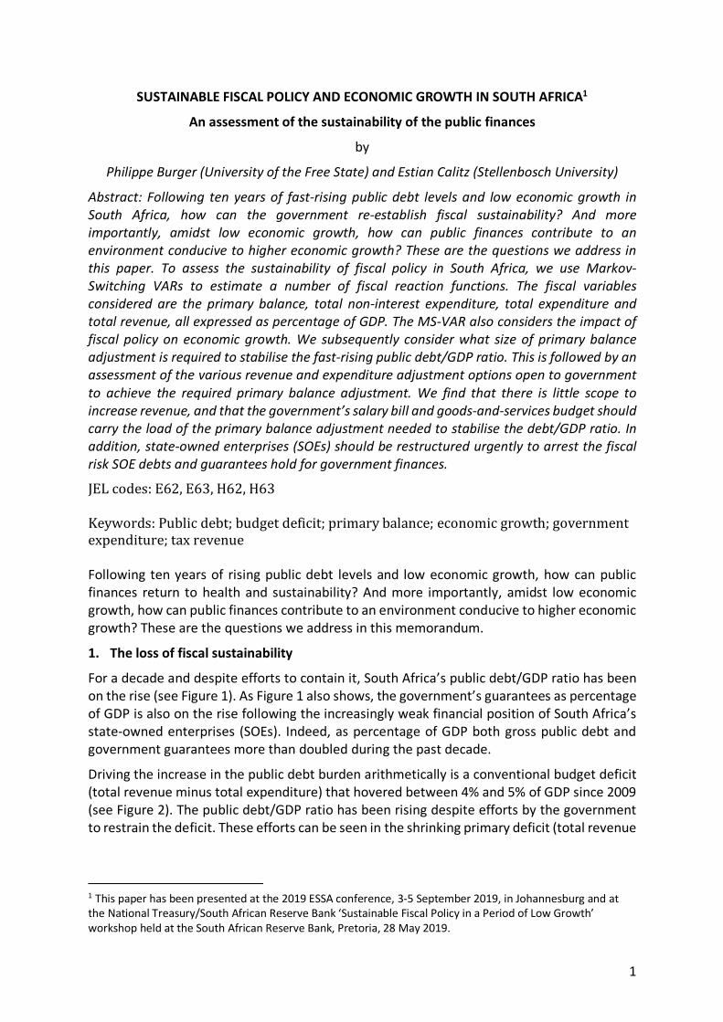
For a decade and despite efforts to contain it, South Africa’s public debt/GDP ratio has been on the rise (see Figure 1). As Figure 1 also shows, the government’s guarantees as percentage of GDP is also on the rise following the increasingly weak financial position of South Africa’s state-owned enterprises (SOEs). Indeed, as percentage of GDP both gross public debt and government guarantees more than doubled during the past decade.
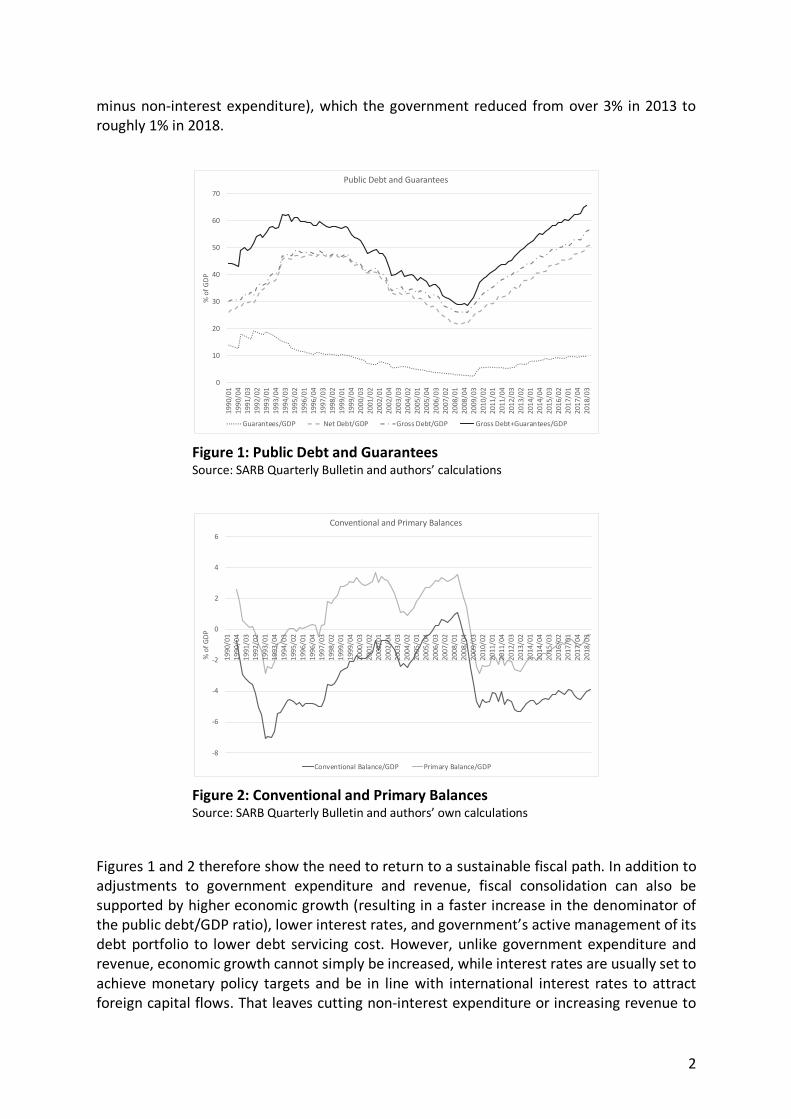
Driving the increase in the public debt burden arithmetically is a conventional budget deficit (total revenue minus total expenditure) that hovered between 4% and 5% of GDP since 2009 (see Figure 2). The public debt/GDP ratio has been rising despite efforts by the government to restrain the deficit. These efforts can be seen in the shrinking primary deficit (total revenue
1 This paper has been presented at the 2019 ESSA conference, 3-5 September 2019, in Johannesburg and at the National Treasury/South African Reserve Bank ‘Sustainable Fiscal Policy in a Period of Low Growth’ workshop held at the South African Reserve Bank, Pretoria, 28 May 2019.
2
minus non-interest expenditure), which the government reduced from over 3% in 2013 to roughly 1% in 2018.
Figure 1: Public Debt and Guarantees Source: SARB Quarterly Bulletin and authors’ calculations
Figure 2: Conventional and Primary Balances Source: SARB Quarterly Bulletin and authors’ own calculations
Figures 1 and 2 therefore show the need to return to a sustainable fiscal path. In addition to adjustments to government expenditure and revenue, fiscal consolidation can also be supported by higher economic growth (resulting in a faster increase in the denominator of the public debt/GDP ratio), lower interest rates, and government’s active management of its debt portfolio to lower debt servicing cost. However, unlike government expenditure and revenue, economic growth cannot simply be increased, while interest rates are usually set to achieve monetary policy targets and be in line with international interest rates to attract foreign capital flows. That leaves cutting non-interest expenditure or increasing revenue to
0
10
20
30
40
50
60
70
1990
/01
1990
/04
1991
/03
1992
/02
1993
/01
1993
/04
1994
/03
1995
/02
1996
/01
1996
/04
1997
/03
1998
/02
1999
/01
1999
/04
2000
/03
2001
/02
2002
/01
2002
/04
2003
/03
2004
/02
2005
/01
2005
/04
2006
/03
2007
/02
2008
/01
2008
/04
2009
/03
2010
/02
2011
/01
2011
/04
2012
/03
2013
/02
2014
/01
2014
/04
2015
/03
2016
/02
2017
/01
2017
/04
2018
/03
% o
f GDP
Public Debt and Guarantees
Guarantees/GDP Net Debt/GDP Gross Debt/GDP Gross Debt+Guarantees/GDP
-8
-6
-4
-2
0
2
4
6
1990
/01
1990
/04
1991
/03
1992
/02
1993
/01
1993
/04
1994
/03
1995
/02
1996
/01
1996
/04
1997
/03
1998
/02
1999
/01
1999
/04
2000
/03
2001
/02
2002
/01
2002
/04
2003
/03
2004
/02
2005
/01
2005
/04
2006
/03
2007
/02
2008
/01
2008
/04
2009
/03
2010
/02
2011
/01
2011
/04
2012
/03
2013
/02
2014
/01
2014
/04
2015
/03
2016
/02
2017
/01
2017
/04
2018
/03
% o
f GDP
Conventional and Primary Balances
Conventional Balance/GDP Primary Balance/GDP

3
achieve fiscal sustainability as primary instruments to attain fiscal sustainability. Nevertheless, in principle, doing so might negatively impact economic growth, creating the danger that efforts to arrest the increase in the public debt/GDP ratio become self-defeating (e.g. even though cutting the deficit ensures that the public debt increases more slowly, if cutting the deficit also depresses economic growth, the denominator in the debt/GDP ratio might also increase more slowly, thereby leaving the overall ratio unchanged or even increasing – the experience of Greece in the last decade is often held as an example of this phenomenon). Though this is a possibility, what does international literature conclude are the best channels to effect fiscal consolidation?
2. Empirical evidence on successful fiscal consolidation
International literature considers the question ‘what constitutes a durable consolidation?’, with ‘durable’ meaning less likely to have been reversed within a few years after satisfying the chosen criteria for a successful consolidation. The literature shows that in OECD countries cuts in transfer payments and the government wage bill were more likely to have achieved significant and durable reductions in fiscal deficits than those based mainly on tax increases (Alesina and Ardagna, 1998; 2010; 2013; Alesina and Perotti, 1997; Ardagna, 2004; Guichard, Kennedy, Wurzel and André, 2007; McDermott and Wescott, 1996; Von Hagen and Strauch, 2001). Wiese, Jong-A-Pin and De Haan (2018) found that a fiscal adjustment’s success improves if a left-wing government relies on spending cuts and a right-wing government relies on tax increases.
Kickert et al (2015) argue that cutbacks on operational costs (hiring and pay freeze, wage reduction, staff reduction) followed a similar pattern across Europe. Virtually no country undergoing a successful fiscal adjustment could escape a freeze on hiring and pay, or capping replacements. Nevertheless, in most countries, governments introduced politically sensitive measures such as reducing wages and employment only in the later stages of the crisis. However, European countries that received bail-outs on condition of cuts to their public sector wage bill did apply immediate cuts in salaries and employment. Hardiman, Dellepiane and Hardiman (2015: 28) investigated fiscal consolidation in Ireland, Greece, Britain and Spain (1980 to 2012) and found that older literature on fiscal consolidation from the 1990s and 2000s overlooked core issues in domestic political economy, including the role of interest group representation, political legitimacy, and policy contestation. Without bringing in politics – including the new politics of multi-level economic governance – the analysis of credibility and efficacy in fiscal consolidation policies is unlikely to deliver plausible policy advice. (Also see Figari & Fiori, 2015: 15).
Furthermore, Baldacci, Clements, Gupta and Mulas-Granados (2004) and Gupta, Baldacci, Clements and Tiongson (2003) found that protecting or increasing the share of capital spending in total government expenditure during consolidation episodes increased the probabilities of success and persistence. In some OECD countries taxes played a role as well, e.g. VAT increases in the Eurozone during the international financial crisis had an impact, but also displayed adverse distributional implications (de Mooij and Keen, 2013).
In emerging market countries, the empirical literature also links success and persistence of fiscal consolidations to the extent that the government cuts back current expenditure (cf. Adam and Bevan, 2003; Baldacci, Clements, Gupta and Mulas-Granados, 2004; 2006; Gupta et al., 2003; Gupta, Clements, Baldacci and Mulas-Granados, 2004). The art of cutbacks also requires a serious and continuous review of all expenditure so as to ensure that the

4
prioritisation of public spending programmes contributes to allocative efficiency. There must also be collective responsibility for and commitment in government for this approach – in the national interest rather than sectional interests.
To a larger extent than in OECD countries revenue increases also played a role in successfully consolidating fiscal positions. But this mostly occurred in cases where revenue collection was weak and where large tax gaps existed. Thus, in emerging market and developing economies revenue contributed to fiscal consolidation where there was considerable scope to increase tax revenues without raising tax rates (i.e. improve tax administration).
3. Empirical findings for South Africa
What has been the behaviour of fiscal policy in South Africa? Did the government take steps to re-establish fiscal sustainability and arrest the increase in the debt/GDP ratio (this is usually done by increasing the primary balance in reaction to an increase in the debt/GDP ratio)? And what has been the impact of fiscal policy on economic growth? To explore these questions, we conducted an empirical analysis.
3.1 Economic growth and the sustainability of fiscal policy
Fiscal reaction functions have their origin in the work of Henning Bohn (1995; 1998; 2007; 2010). To establish whether or not fiscal policy reacts to an increase in the debt/GDP ratio, the primary balance/GDP ratio (𝐵"/𝑌" in Equation 1) is regressed on a lag of the debt/GDP ratio (𝐷"&'/𝑌"&' in Equation 1). The question is whether 𝛽' in Equation 1 is positive, i.e. if (𝐷"&'/𝑌"&') increases, the primary balance increases in period t:
𝐵"/𝑌" = 𝛽- + 𝜷𝟏(𝑫𝒕&𝟏/𝒀𝒕&𝟏) + 𝛽4𝑔"&'+𝛽6𝐵"&'/𝑌"&' + 𝜀" (1)
Where:
• 𝐵"/𝑌" is the primary balance (surplus (+)/deficit (-)) • 𝐷"&'/𝑌"&' is the debt/GDP ratio • g is the economic growth rate, its inclusion measures a business cycle reaction, i.e. if 𝛽4 is
negative lower growth leads to a more stimulating fiscal policy. • 𝐵"&'/𝑌"&' is included to allow for inertia in government’s behaviour.
The primary balance is difference between non-interest expenditure and revenue. Thus, if it is found that the government changes the primary balance/GDP ratio in reaction to changes in the debt/GDP ratio, the question is whether the government reduced the total non-interest expenditure/GDP ratio or increased the total revenue/GDP ratio (or both) in reaction to an increase in the debt/GDP ratio. Since the government can also manage its interest bill down in reaction to an increase in the debt/GDP ratio, we also considered the reaction of total expenditure to a change in the debt/GDP ratio. Thus, following Claeys (2008) and Favero and Marcellino (2005) we also estimated the following regressions:
𝑁𝐼𝐸"/𝑌" = 𝛽- + 𝛽'(𝐷"&'/𝑌"&') + 𝛽4𝑔"&'+𝛽6𝑁𝐼𝐸"&'/𝑌"&' + 𝜀" (2)
𝐸"/𝑌" = 𝛽- + 𝛽'(𝐷"&'/𝑌"&') + 𝛽4𝑔"&'+𝛽6𝐸"&'/𝑌"&' + 𝜀" (3)
𝑇"/𝑌" = 𝛽- + 𝛽'(𝐷"&'/𝑌"&') + 𝛽4𝑔"&'+𝛽6𝑇"&'/𝑌"&' + 𝜀" (4)

5
We expect 𝛽' to be negative in Equations (2) and (3) and positive in Equation (4). Equations (1) to (4) were each estimated in a model that also contained a version of Equation (5). Thus, we estimated the a Vector Autoregressive (VAR) Model.
𝑔" = 𝛽- + 𝛽'(𝐷"&'/𝑌"&') + 𝛽4𝑔"&'+𝛽6𝐹"&'/𝑌"&' + 𝜀" (5)
Where 𝐹"&'/𝑌"&' is the fiscal variable used in that model. Thus, in the model estimated with the primary balance 𝐹"&'/𝑌"&' is 𝐵"&'/𝑌"&', while in the other models it is respectively 𝑁𝐼𝐸"&'/𝑌"&', 𝐸"&'/𝑌"&', and 𝑇"&'/𝑌"&'. Lastly, to allow for two behavioural regimes of fiscal policy, we used the Markov-switching methodology to estimate the VAR (see Ricci-Risquete, Ramajo, and De Castro (2016) who also used an MS-VAR model for Spain).
3.1.1 Primary balance reaction functions
The primary balance/GDP ratio reacts to an increase in the debt/GDP ratio. The reaction has the appropriate sign. A one percentage point increase in the debt/GDP ratio leads to a 0.012 percentage point increase in the primary balance/GDP ratio.
Figure A1: Regime-switching behaviour in the primary balance/GDP and economic growth model
Although this regression shows that the primary balance/GDP ratio reacted throughout the sample period, the constant of -0.742 in Regime 1 is lower than the statistically insignificant constant value of -0.193 in regime 0. This means that the average primary balance/GDP ratio during Regime 1 (in place since 2009Q2) has been too low to prevent an increase in the debt/GDP ratio. The estimation detects no impact of the primary balance/GDP ratio on economic growth.

6
Table 1: Primary balance to debt reaction function Primary Balance/GDP GDP growth Primary Balance/GDP (t-1) 0.866 (0.000) -0.039 (0.757) Primary Balance/GDP (t-2) 0.250 (0.034) -0.069 (0.684) Primary Balance/GDP (t-3) -0.269 (0.001) 0.024 (0.830) GDP growth (t-1) 0.170 (0.003) 0.499 (0.000) Debt/GDP (t-4) 0.012 (0.021) -0.003 (0.734) Constant (0) -0.193 (0.424) 0.768 (0.028) Constant (1) -0.742 (0.001) 0.226 (0.475) Linearity LR-test Chi^2(4) 226.59 (0.000) Vector Normality test Chi^2(4) 4.587 (0.332) Vector ARCH 1-1 test F(4,174) 0.224 (0.925) Vector Portmanteau(12) Chi^2(44) 45.99 (0.390) Transition probabilities Regime 0,t Regime 1,t Regime 0,t+1 0.972 0.017 Regime 1,t+1 0.028 0.983 Regime 0 Quarters Average probability 1997(3) - 2008(2) 44 0.981 Regime 1 Quarters Average probability 1991(3) - 1997(2) 24 0.987 2008(3) - 2018(4) 42 0.998
Other coefficients (Std Error): scale[0] 0.502 (0.035); scale[1] 0.342 (0.024); L[1][0] -0.069 (0.066); p{0|0} 0.972 (0.028); p{1|1} 0.984 (0.017) Probabilities ( ); Sample: 1991(3) - 2018(4) Regime 0: Total: 44 quarters (40.00%) with average duration of 44.00 quarters. Regime 1: Total: 66 quarters (60.00%) with average duration of 33.00 quarters. 3.1.2 Total non-interest expenditure reaction functions
Two regimes were identified with respect to the reaction of the total non-interest expenditure/GDP ratio to specifically changes in the debt/GDP ratio. Regime 0 has existed from 2009Q2, while Regime 1 existed from 1997Q3 to 2009Q1.
Figure A2: Regime-switching behaviour in the total non-interest expenditure/GDP and economic growth model

7
In Regime 1 total non-interest expenditure does not react to increases in the debt/GDP ratio, which also helps to explain why the debt/GDP ratio kept increasing from 2009Q2. In Regime 0, which existed from 1997Q3 to 2009Q1, total non-interest expenditure did react to increases in the debt/GDP ratio; with the non-interest expenditure/GDP ratio falling by 0.032 percentage point for every percentage point increase in the debt/GDP ratio. This partially explains the reduction in the debt/GDP ratio in the 2000s. In addition, the non-interest expenditure/GDP ratio falls in reaction to an increase in the growth rate, with the fall being larger in Regime 0 (2009Q2 to 2018Q4) than in Regime 1 (1997Q3 to 2009Q1) – unfortunately average growth during Regime 1 has been much lower than during Regime 0.
Table A2: Total non-interest expenditure to debt reaction function
Total Non-interest Expenditure/GDP GDP growth Total NI Exp/GDP (t-1) 0.865 (0.000) -0.060 (0.147) GDP growth (t-1) (0) -0.237 (0.000) 0.220 (0.056) GDP growth (t-1) (1) -0.109 (0.027) 0.810 (0.000) Debt/GDP (t-4) (0) -0.007 (0.104) -0.014 (0.119) Debt/GDP (t-4) (1) -0.032 (0.000) 0.010 (0.278) Constant (0) 3.969 (0.000) 2.474 (0.023) Constant (1) 4.175 (0.000) 0.970 (0.367) Linearity LR-test Chi^2(4) 288.21 (0.000) Vector Normality test Chi^2(4) 5.368 (0.252) Vector ARCH 1-1 test F(4,174) 0.585 (0.674) Vector Portmanteau(12) Chi^2(44) 48.48 (0.413) Transition probabilities Regime 0,t Regime 1,t Regime 0,t+1 0.949 0.048 Regime 1,t+1 0.051 0.952 Regime 0 Quarters Average probability 1993(1) - 1993(1) 1 1.000 1996(3) - 1997(2) 4 0.999 2009(2) - 2018(4) 39 0.999 Regime 1 Quarters Average probability 1991(4) - 1992(4) 5 1.000 1993(2) - 1996(2) 13 0.980 1997(3) - 2009(1) 47 0.993
Other coefficients (Std Error): scale[0] 0.475 (0.032); scale[1] 0.243 (0.017); L[1][0] -0.011 (0.052); p{0|0} 0.949 (0.035); p{1|1} 0.952 (0.028) Probabilities ( ); Sample: 1991(4) - 2018(4) Regime 0: Total: 44 quarters (40.37%) with average duration of 14.67 quarters. Regime 1: Total: 65 quarters (59.63%) with average duration of 21.67 quarters.
3.1.3 Total expenditure reaction functions
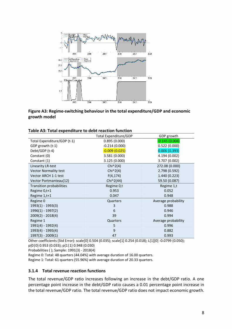
An increase in the debt/GDP ratio leads to a reduction in the total government expenditure/GDP ratio. In addition, an increase in economic growth leads to a reduction in the total government expenditure/GDP ratio. Furthermore, an increase in the total government expenditure/GDP ratio leads to a reduction in economic growth. Specifically, a one percentage point increase in the total government expenditure/GDP ratio leads to a reduction in economic growth of 0.145 percentage points. In addition, an increase in the economic growth rate leads to a reduction in the total expenditure/GDP ratio.
8
Figure A3: Regime-switching behaviour in the total expenditure/GDP and economic growth model
Table A3: Total expenditure to debt reaction function
Total Expenditure/GDP GDP growth Total Expenditure/GDP (t-1) 0.895 (0.000) -0.145 (0.004) GDP growth (t-1) -0.214 (0.000) 0.522 (0.000) Debt/GDP (t-4) -0.009 (0.025) 0.006 (0.393) Constant (0) 3.581 (0.000) 4.194 (0.002) Constant (1) 3.125 (0.000) 3.707 (0.002) Linearity LR-test Chi^2(4) 272.08 (0.000) Vector Normality test Chi^2(4) 2.798 (0.592) Vector ARCH 1-1 test F(4,174) 1.440 (0.223) Vector Portmanteau(12) Chi^2(44) 59.50 (0.087) Transition probabilities Regime 0,t Regime 1,t Regime 0,t+1 0.953 0.052 Regime 1,t+1 0.047 0.948 Regime 0 Quarters Average probability 1993(1) - 1993(3) 3 0.988 1996(1) - 1997(2) 6 0.946 2009(2) - 2018(4) 39 0.994 Regime 1 Quarters Average probability 1991(4) - 1992(4) 5 0.996 1993(4) - 1995(4) 9 0.882 1997(3) - 2009(1) 47 0.993
Other coefficients (Std Error): scale[0] 0.504 (0.035); scale[1] 0.254 (0.018); L[1][0] -0.0799 (0.050); p{0|0} 0.953 (0.033); p{1|1} 0.948 (0.030) Probabilities ( ); Sample: 1991(3) - 2018(4) Regime 0: Total: 48 quarters (44.04%) with average duration of 16.00 quarters. Regime 1: Total: 61 quarters (55.96%) with average duration of 20.33 quarters. 3.1.4 Total revenue reaction functions
The total revenue/GDP ratio increases following an increase in the debt/GDP ratio. A one percentage point increase in the debt/GDP ratio causes a 0.01 percentage point increase in the total revenue/GDP ratio. The total revenue/GDP ratio does not impact economic growth.

9
Figure A4: Regime-switching behaviour in the total revenue/GDP and economic growth model
Table A4: Revenue to debt reaction function Total Revenue/GDP GDP growth Total Revenue/GDP (t-1) 1.088 (0.000) 0.008 (0.943) Total Revenue/GDP (t-3) -0.217 (0.000) -0.121 (0.262) GDP growth (t-1) 0.034 (0.387) 0.533 (0.000) Debt/GDP (t-4) 0.010 (0.008) 0.001 (0.932) Constant (0) 2.798 (0.001) 2.999 (0.047) Constant (1) 2.421 (0.001) 2.796 (0.039) Linearity LR-test Chi^2(4) 296.76 (0.000) Vector Normality test Chi^2(4) 5.729 (0.220) Vector ARCH 1-1 test F(4,174) 1.170 (0.326) Vector Portmanteau(12) Chi^2(44) 49.12 (0.312) Transition probabilities Regime 0,t Regime 1,t Regime 0,t+1 1.000 0.019 Regime 1,t+1 0.000 0.981 Regime 0 Quarters Average probability 2004(4) - 2018(4) 57 0.995 Regime 1 Quarters Average probability 1991(4) - 2004(3) 52 0.982
Other coefficients (Std Error): scale[0] 0.516 (0.035); scale[1] 0.249 (0.017); L[1][0] -0.000 (0.047); p{1|1} 0.981 (0.019) Probabilities ( ); Sample: 1991(4) - 2018(4) Regime 0: Total: 57 quarters (52.29%) with average duration of 57.00 quarters. Regime 1: Total: 52 quarters (47.71%) with average duration of 52.00 quarters.
3.2 Summary of empirical findings
With regard to the reaction of fiscal policy to changes in debt/GDP:
• When the public debt/GDP ratio increased during the period 1991 to 2018, the government, in reaction, increased the primary balance/GDP ratio in an attempt to arrest the increase in the debt/GDP ratio (and the opposite when the debt/GDP ratio fell). Notwithstanding this reaction, what the analysis also shows is that since the third quarter of 2008 the overall level of the primary balance was too low to prevent an increase in the

10
debt/GDP ratio. Thus, although fiscal policy took steps to arrest the increase in the debt/GDP ratio, since 2008 those steps were just not enough.
• When the public debt/GDP ratio increased during the period 1991 to 2018, the government, in reaction, increased the total revenue/GDP ratio. However, total non-interest expenditure/GDP has not reacted to changes in the debt/GDP ratio since the second quarter of 2009. Thus, the reaction observed in the primary balance/GDP ratio to changes in the debt/GDP ratio during the last decade, is due to the reaction of revenue/GDP, not non-interest expenditure. In short, though it failed to stabilise the debt/GDP ratio revenue, revenue did the work of preventing the debt/GDP ratio from increasing any faster.
With regard to the impact of fiscal policy on economic growth:
• Increases in the debt/GDP ratio in the period 1991-2018 did not impact economic growth negatively.
• Changes in the primary deficit/GDP, total non-interest expenditure/GDP and total revenue/GDP in the period 1991-2018 did not impact on economic growth
• Increases in total expenditure/GDP in the period 1991-2018 did impact economic growth negatively. This means that higher levels of government expenditure relative to GDP dampen economic growth. The reverse is also true, should the government reduce the total expenditure/GDP ratio, it will lead to higher economic growth. The regression analysis does not consider the various channels through which this may occur, but typically lower levels of government expenditure might release resources for private investment (thus, the crowding-out process in reverse), while any negative multiplier effect resulting directly from the reduction in government expenditure might be offset by a positive confidence and multiplier effect of higher private investment and consumption expenditure. All of this does not exclude the possible growth-enhancing impact of improvements in the allocative efficiency of government programmes, for any given aggregate expenditure level.
4. What size of fiscal adjustment is required?
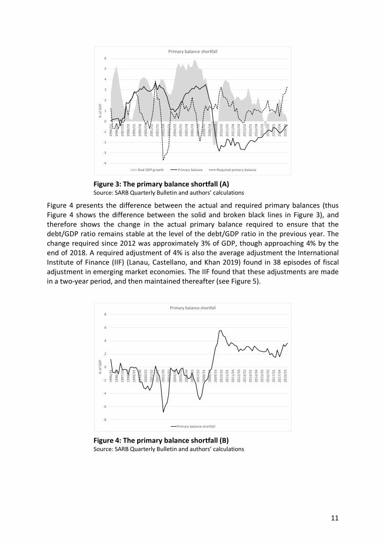
The above analysis shows what the fiscal adjustment was in the past. This section briefly sets out the requirements for future adjustment. Figure 3 contrasts the actual primary balance/GDP ratio (solid black line) in each year with the primary balance/GDP ratio that was required in each year to stabilise the debt/GDP ratio at its level in the previous year (broken black line) – thus, the debt/GDP ratio used to calculate the required primary balance is a moving target; each year it is reset at the level of the actual debt/GDP ratio of the previous year. Figure 3 shows that from 1999 to 2008 the actual primary balance/GDP ratio exceeded the required primary balance/GDP ratio, which explains why the debt/GDP ratio fell during this period (see Figure 1 above). The reverse holds for the period since 2009.
11
Figure 3: The primary balance shortfall (A) Source: SARB Quarterly Bulletin and authors’ calculations
Figure 4 presents the difference between the actual and required primary balances (thus Figure 4 shows the difference between the solid and broken black lines in Figure 3), and therefore shows the change in the actual primary balance required to ensure that the debt/GDP ratio remains stable at the level of the debt/GDP ratio in the previous year. The change required since 2012 was approximately 3% of GDP, though approaching 4% by the end of 2018. A required adjustment of 4% is also the average adjustment the International Institute of Finance (IIF) (Lanau, Castellano, and Khan 2019) found in 38 episodes of fiscal adjustment in emerging market economies. The IIF found that these adjustments are made in a two-year period, and then maintained thereafter (see Figure 5).
Figure 4: The primary balance shortfall (B) Source: SARB Quarterly Bulletin and authors’ calculations
-4
-3
-2
-1
0
1
2
3
4
5
6
1996
/01
1996
/04
1997
/03
1998
/02
1999
/01
1999
/04
2000
/03
2001
/02
2002
/01
2002
/04
2003
/03
2004
/02
2005
/01
2005
/04
2006
/03
2007
/02
2008
/01
2008
/04
2009
/03
2010
/02
2011
/01
2011
/04
2012
/03
2013
/02
2014
/01
2014
/04
2015
/03
2016
/02
2017
/01
2017
/04
2018
/03
% o
f GDP
Primary balance shortfall
Real GDP growth Primary balance Required primary balance
-8
-6
-4
-2
0
2
4
6
8
1996
/01
1996
/04
1997
/03
1998
/02
1999
/01
1999
/04
2000
/03
2001
/02
2002
/01
2002
/04
2003
/03
2004
/02
2005
/01
2005
/04
2006
/03
2007
/02
2008
/01
2008
/04
2009
/03
2010
/02
2011
/01
2011
/04
2012
/03
2013
/02
2014
/01
2014
/04
2015
/03
2016
/02
2017
/01
2017
/04
2018
/03
% o
f GDP
Primary balance shortfall
Primary balance shortfall

12
KES: Kenya; RSD: Serbia; JMD: Jamaica; LKR: Sri Lanka; JOD: Jordan; EGP: Egypt; ARS: Argentina Figure 5: Primary balance adjustments in emerging markets Source: Adapted from Lanau, Castellano, Khan (2019)
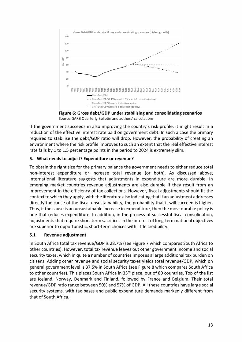
What should be the adjustment path of fiscal policy in South Africa? To explore a realistic adjustment path Table 1 and Figure 8 present two adjustment paths. The first, Scenario 1, is a stabilising fiscal policy that aims at merely arresting the increase in the gross debt GDP ratio, keeping it stable afterwards, while the second, Scenario 2, is a consolidating fiscal policy that seeks to reduce the gross debt/GDP ratio to below 40% by the mid-2030s. Table 1 shows the assumptions made. It shows that for both policies we assume that the economic growth rate slowly improves to a modest 2.5% by 2023. In the case of the stabilising policy the primary balance improves from a deficit of 1% of GDP in 2019 to a surplus of 1% by 2021. Note that the adjustment is smaller than the adjustment identified in Figure 4 above because in Table 1 and Figure 6 we assume that the economic growth rate improves by 1.5 percentage points. In the case of the consolidating policy the primary balance improves from a primary deficit of 1% of GDP in 2019 to a primary surplus of 2.5% of GDP by 2023.
Table 1: Stabilising as well as consolidating fiscal policy – assumptions made Current trajectory Scenario 1:
Stabilising policy Scenario 2:
Consolidating policy Primary balance -1.5% 2019: -1%
2020: 0% 2021: 1% 2022: 1% 2023: 1%
2024 onwards: 1%
2019: -1% 2020: 0% 2021: 1%
2022: 1.5% 2023: 2%
2024 onwards: 2.5% Real interest rate 4% 4% 4% Real growth rate 1.45% 2019: 1%
2020: 1.5% 2021: 2% 2022: 2%
2023 onwards: 2.5%
2019: 1% 2020: 1.5% 2021: 2% 2022: 2%
2023 onwards:2.5%
13
Figure 6: Gross debt/GDP under stabilising and consolidating scenarios Source: SARB Quarterly Bulletin and authors’ calculations
If the government succeeds in also improving the country’s risk profile, it might result in a reduction of the effective interest rate paid on government debt. In such a case the primary required to stabilise the debt/GDP ratio will drop. However, the probability of creating an environment where the risk profile improves to such an extent that the real effective interest rate falls by 1 to 1.5 percentage points in the period to 2024 is extremely slim.
5. What needs to adjust? Expenditure or revenue?
To obtain the right size for the primary balance the government needs to either reduce total non-interest expenditure or increase total revenue (or both). As discussed above, international literature suggests that adjustments in expenditure are more durable. In emerging market countries revenue adjustments are also durable if they result from an improvement in the efficiency of tax collections. However, fiscal adjustments should fit the context to which they apply, with the literature also indicating that if an adjustment addresses directly the cause of the fiscal unsustainability, the probability that it will succeed is higher. Thus, if the cause is an unsustainable increase in expenditure, then the most durable policy is one that reduces expenditure. In addition, in the process of successful fiscal consolidation, adjustments that require short-term sacrifices in the interest of long-term national objectives are superior to opportunistic, short-term choices with little credibility.
5.1 Revenue adjustment
In South Africa total tax revenue/GDP is 28.7% (see Figure 7 which compares South Africa to other countries). However, total tax revenue leaves out other government income and social security taxes, which in quite a number of countries imposes a large additional tax burden on citizens. Adding other revenue and social security taxes yields total revenue/GDP, which on general government level is 37.5% in South Africa (see Figure 8 which compares South Africa to other countries). This places South Africa in 33rd place, out of 80 countries. Top of the list are Iceland, Norway, Denmark and Finland, followed by France and Belgium. Their total revenue/GDP ratio range between 50% and 57% of GDP. All these countries have large social security systems, with tax bases and public expenditure demands markedly different from that of South Africa.
0
20
40
60
80
100
120
140
2000
2001
2002
2003
2004
2005
2006
2007
2008
2009
2010
2011
2012
2013
2014
2015
2016
2017
2018
2019
2020
2021
2022
2023
2024
2025
2026
2027
2028
2029
2030
2031
2032
2033
2034
2035
2036
% o
f GDP
Gross Debt/GDP under stabilising and consolidating scenarios (higher growth)
Gross Debt/GDP
Gross Debt/GDP (1.45% growth, 1.5% prim def, current trajectory)
Gross Debt/GDP (Scenario 1: stabilising policy)Gross Debt/GDP (Scenario 2: consolidating policy)

14
Figure 7: General government total tax as percentage of GDP Source: IMF
Figure 9: General government total revenue as percentage of GDP Source: IMF
Of the 32 countries with heavier total revenue burdens than South Africa, 22 are OECD countries and four are Eastern European transition economies with higher per capita GDPs than South Africa. South Africa is highly taxed for an emerging market. Only five emerging economies carry heavier burdens: Brazil, Cyprus, Tonga, Malta and the Seychelles. There are
15
20 emerging markets which collect less revenue as percentage of GDP than SA, including China, Thailand, Indonesia, Kenya and Uganda. South Africa also has a higher total revenue/GDP ratio than the US, Switzerland, South Korea, Australia and Israel, all of which are developed economies. Although the empirical analysis reported above found that an increase in the total revenue/GDP ratio did not impact negatively on GDP in the period 1991 to 2018, given South Africa’s relatively high revenue burden compared to other emerging market economies, there is little scope for South Africa to increase tax rates in future. Doing so will serve as a disincentive for individuals and companies to earn their income and be taxed in South Africa.
5.2 Capital expenditure adjustment
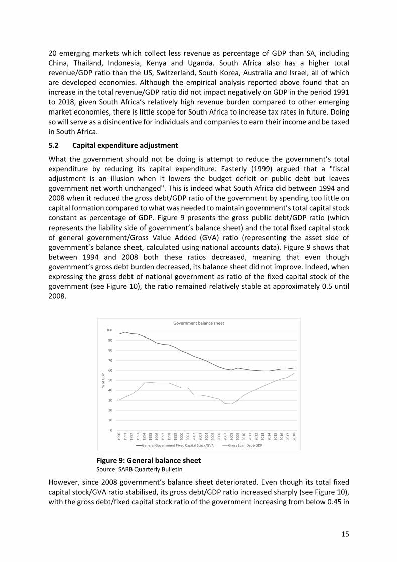
What the government should not be doing is attempt to reduce the government’s total expenditure by reducing its capital expenditure. Easterly (1999) argued that a "fiscal adjustment is an illusion when it lowers the budget deficit or public debt but leaves government net worth unchanged". This is indeed what South Africa did between 1994 and 2008 when it reduced the gross debt/GDP ratio of the government by spending too little on capital formation compared to what was needed to maintain government’s total capital stock constant as percentage of GDP. Figure 9 presents the gross public debt/GDP ratio (which represents the liability side of government’s balance sheet) and the total fixed capital stock of general government/Gross Value Added (GVA) ratio (representing the asset side of government’s balance sheet, calculated using national accounts data). Figure 9 shows that between 1994 and 2008 both these ratios decreased, meaning that even though government’s gross debt burden decreased, its balance sheet did not improve. Indeed, when expressing the gross debt of national government as ratio of the fixed capital stock of the government (see Figure 10), the ratio remained relatively stable at approximately 0.5 until 2008.
Figure 9: General balance sheet Source: SARB Quarterly Bulletin
However, since 2008 government’s balance sheet deteriorated. Even though its total fixed capital stock/GVA ratio stabilised, its gross debt/GDP ratio increased sharply (see Figure 10), with the gross debt/fixed capital stock ratio of the government increasing from below 0.45 in
0
10
20
30
40
50
60
70
80
90
100
1990
1991
1992
1993
1994
1995
1996
1997
1998
1999
2000
2001
2002
2003
2004
2005
2006
2007
2008
2009
2010
2011
2012
2013
2014
2015
2016
2017
2018
% o
f GDP
Government balance sheet
General Government Fixed Capital Stock/GVA Gross Loan Debt/GDP

16
2008 to over 0.9 in 2018 (see Figure 10). Cutting capital expenditure to reduce the debt burden might again, to a limited extent (limited because government’s capital budget is small relative to its total expenditure) assist in reducing the debt burden, but the fall in the debt burden will not improve government’s balance sheet.
Figure 10: Gross loan debt (national government)/Capital stock (general
government) Source: SARB Quarterly Bulletin
Figure 11: SOE balance sheet Source: SARB Quarterly Bulletin
In addition, due to the previous episode during which the government reduced its debt burden by allowing its fixed capital stock/GVA ratio to deteriorate, South Africa’s public infrastructure is under pressure. Not only did the general government’s fixed capital stock/GVA ratio decrease until 2008, but so too did the total non-financial assets/GDP ratio of state-owned enterprises decrease (a similar decrease occurred in the private sector’s fixed capital stock/GVA ratio). This also put pressure on public infrastructure (see Figure 11). Not only does a reduction of the public debt burden attained through the deterioration in the government’s fixed capital/GVA ratio not improve the government’s balance sheet, but it also
0.00
0.10
0.20
0.30
0.40
0.50
0.60
0.70
0.80
0.90
1.0019
9019
9119
9219
9319
9419
9519
9619
9719
9819
9920
0020
0120
0220
0320
0420
0520
0620
0720
0820
0920
1020
1120
1220
1320
1420
1520
1620
1720
18
Ratio
Gross loan debt (National Government)/Capital stock ratio (General Government)
Gross loan debt/Capital stock ratio
0
10
20
30
40
50
60
1981
1982
1983
1984
1985
1986
1987
1988
1989
1990
1991
1992
1993
1994
1995
1996
1997
1998
1999
2000
2001
2002
2003
2004
2005
2006
2007
2008
2009
2010
2011
2012
2013
2014
2015
2016
2017
2018
% o
f GD
P
SOE sector balance sheet
Total Non-Financial Assets/GDP Total Debt/GDP
Total Debt + Other Accounts Payable/GDP Equity/GDP

17
undermines the longer-run growth capacity of the economy. Lower growth in the longer run also undermines the sustainability of fiscal policy as it undermines the revenue earning capacity of the government.
Since 2008 the total non-financial assets/GDP ratio of SOEs improved to over 30%, largely because of the construction of the Medupi and Kusile power plants. However, given that these plants operate currently only at 40%, are still not complete and suffer from major construction errors and management deficiencies, the increase in the total non-financial assets/GDP ratio is probably inflated. If it is inflated, the true value of the SOE equity/GDP ratio might be much lower than reported in Figure 11. Instead of the reported increase, it might have decreased since 2008. The increased total-debt-and-other-accounts-payable/GDP ratio is also reflected in the increased guarantees/GDP ratio reported in Figure 1 and constitutes one of the largest fiscal risks the South African government faces in 2019. Moody’s already in May 2019 announced that in assessing the country’s sovereign credit rating they will consider the public debt/GDP burden inclusive of guarantees. As Figure 1 above shows, the gross public debt-plus-guarantees ratio is in excess of 65% in 2019. With SOE debt as well as guarantees more than doubling as percentages of GDP since 2008, restructuring the finances of SOEs is key to ensure fiscal sustainability.
Not only has the general government’s own balance sheet deteriorated significantly since 2008, undermining the country’s longer run economic growth potential, so too has that of SOEs, further undermining the country’s longer run economic growth potential. For instance, given the strain on the country’s electricity and water infrastructure, there is little prospect in the foreseeable future of reaching the GEAR, ASGISA and the NDP growth targets of 5% and 6%. Attempting to regain fiscal sustainability and reducing the public debt burden by cutting capital expenditure any further will just limit longer-term growth prospects further.
5.3 Current expenditure adjustment
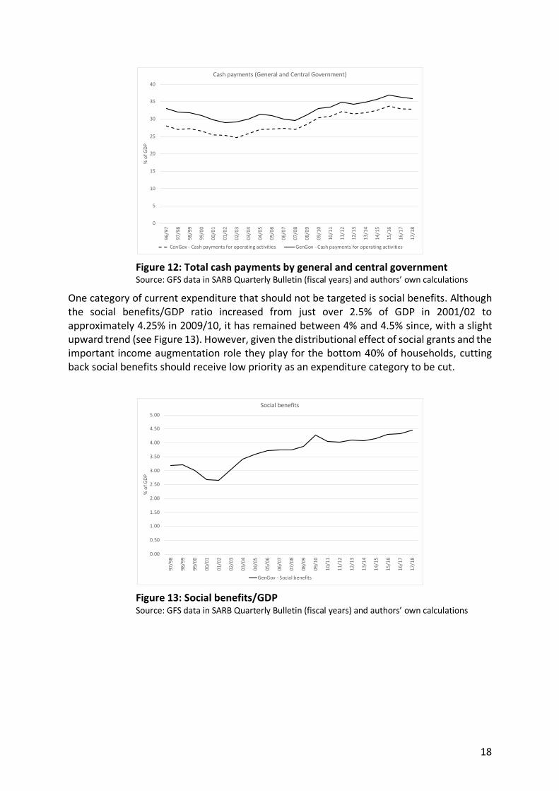
If there is limited scope on the revenue and capital expenditures sides of the budget to adjust the primary balance, the government is left with only the current expenditure side to make the necessary adjustment. Government cash payments for operating activities, on both general and central government level, expressed as percentage of GDP, increased by 7 percentage points between 2007/08 and 2015/06, before tapering off by a percentage point in 2017/08 (see Figure 12). Particularly between 2007/08 and 2011/12 the cash payment for operating activities, as a percentage of GDP, displayed a sharp increase of 5 percentage points, coinciding with the sharp deterioration in the primary balance/GDP ratio observed in Figure 2. Thus, a case exists to address the deterioration in the primary balance by rolling back the increase in government expenditure that gave rise to the deterioration in the first place. In other words, spend only what can be afforded; or, only spend more when it can be afforded.
18
Figure 12: Total cash payments by general and central government Source: GFS data in SARB Quarterly Bulletin (fiscal years) and authors’ own calculations
One category of current expenditure that should not be targeted is social benefits. Although the social benefits/GDP ratio increased from just over 2.5% of GDP in 2001/02 to approximately 4.25% in 2009/10, it has remained between 4% and 4.5% since, with a slight upward trend (see Figure 13). However, given the distributional effect of social grants and the important income augmentation role they play for the bottom 40% of households, cutting back social benefits should receive low priority as an expenditure category to be cut.
Figure 13: Social benefits/GDP Source: GFS data in SARB Quarterly Bulletin (fiscal years) and authors’ own calculations
0
5
10
15
20
25
30
35
40
96/9
7
97/9
8
98/9
9
99/0
0
00/0
1
01/0
2
02/0
3
03/0
4
04/0
5
05/0
6
06/0
7
07/0
8
08/0
9
09/1
0
10/1
1
11/1
2
12/1
3
13/1
4
14/1
5
15/1
6
16/1
7
17/1
8
% o
f GDP
Cash payments (General and Central Government)
CenGov - Cash payments for operating activities GenGov - Cash payments for operating activities
0.00
0.50
1.00
1.50
2.00
2.50
3.00
3.50
4.00
4.50
5.00
97/9
8
98/9
9
99/0
0
00/0
1
01/0
2
02/0
3
03/0
4
04/0
5
05/0
6
06/0
7
07/0
8
08/0
9
09/1
0
10/1
1
11/1
2
12/1
3
13/1
4
14/1
5
15/1
6
16/1
7
17/1
8
% o
f GDP
Social benefits
GenGov - Social benefits

19
Figure 14: Compensation of employees (general and central government) Source: GFS data in SARB Quarterly Bulletin (fiscal years) and authors’ own calculations
Contributing at least 3 percentage points to the increase in the general government expenditure/GDP ratio is compensation of employees, rising from below 11% of GDP in 2007/08 to 14% in 2018 (see Figure 14). On central government level the increase was modest, from just below 4% of GDP in 2007/08, to just below 5% of GDP in 2018. Thus, the sharp increase on general government level occurred at provincial and local government level, which is not surprising given the constitutional structure of subnational responsibilities. Figure 15, which presents the percentage nominal increase in the compensation of employees (i.e. the total salary bill), shows that most of this increase occurred from 2008/09 to 2011/12, with the nominal salary bill in these years increasing in excess of 14%, while both inflation and the nominal percentage increase in GDP were much lower. Since 2012/3 the nominal increase in the salary bill is largely in line with the increase in nominal GDP, which explains why the compensation of employees/GDP ratio stabilised. Nevertheless, the 3-percentage point increase in the compensation of employees/GDP ratio coincided with the between 5% and 6% deterioration in the conventional budget deficit.
Politically reducing the government’s wage bill will be difficult. This emphasises the importance of improving economic growth. As the analysis above has shown, if economic growth improves from 1% to 2.5% by 2023, the required increase in the primary balance decreases from 3% to 2% of GDP. Nevertheless, even with better economic growth, the primary balance must still improve and that improvement will to a large extent have to come from reducing the salary bill. The reduction can also be spread over three or four years to limit the impact per year and allow some of the reduction in the compensation of employees/GDP ratio to come from an increase in its denominator rather than a decrease in its numerator. For more on this, see the recommendation in the conclusion and recommendation section below.
0
2
4
6
8
10
12
14
16
97/9
8
98/9
9
99/0
0
00/0
1
01/0
2
02/0
3
03/0
4
04/0
5
05/0
6
06/0
7
07/0
8
08/0
9
09/1
0
10/1
1
11/1
2
12/1
3
13/1
4
14/1
5
15/1
6
16/1
7
17/1
8
% o
f GDP
Compensation of Employees (General and Central Government)
CenGov - Compensation of employees GenGov - Compensation of employees

20
Figure 15: Government salary bill increase (general government) Source: GFS data in SARB Quarterly Bulletin (fiscal years) and authors’ own calculations
There was also an increase, though much more muted, in the government’s goods-and-services/GDP ratio. It increased from approximately 9.5% in 2008/09 to almost 11% by 2015/16, before returning to just below 10% in 2017/18 (see Figure 16). This ratio can probably be reduced further by improving efficiency and eradicating corruption, and fruitless and wasteful expenditure in government procurement. Improved control over the procurement process of new acquisitions as well as a review of existing contracts to identify overpriced goods and services, will improve value for money. (Incidentally, centralising procurement, while maybe promising some benefits of scale, is not necessarily more efficient in terms of compliance with local requirements, speed of delivery and other controls that are better served in a decentralised manner.) The more value-for-money can be improved through better procurement and the eradication of corruption, the more can be saved on the goods-and-services budget, and the less pressure there is on government’s salary bill to adjust.
Figure 16: Goods and services (general and central government) Source: GFS data in SARB Quarterly Bulletin (fiscal years) and authors’ own calculations
0
2
4
6
8
10
12
14
16
18
20
99/0
0
00/0
1
01/0
2
02/0
3
03/0
4
04/0
5
05/0
6
06/0
7
07/0
8
08/0
9
09/1
0
10/1
1
11/1
2
12/1
3
13/1
4
14/1
5
15/1
6
16/1
7
17/1
8
%
Salary bill and inflation
CPI Inflation (Av for Fiscal years) Compensation of employees (nominal % increase)
GDP (Fiscal years) (nominal % increase)
0
2
4
6
8
10
12
97/9
8
98/9
9
99/0
0
00/0
1
01/0
2
02/0
3
03/0
4
04/0
5
05/0
6
06/0
7
07/0
8
08/0
9
09/1
0
10/1
1
11/1
2
12/1
3
13/1
4
14/1
5
15/1
6
16/1
7
17/1
8
% o
f GDP
Goods and Services (General and Central Government)
CenGov - Goods and services GenGov - Social benefits

21
6. Conclusion and recommendations
To stabilise Debt/GDP requires a 2% of GDP improvement in the primary balance/GDP ratio (and a 2.5% growth rate by 2023). To consolidate the gross debt/GDP to below 40% by 2036 requires a 3.5% of GDP improvement in primary balance/GDP ratio (and also a 2.5% growth rate by 2023). Should economic growth remain stagnant at its average between 2012 and 2018 of 1.45%, the required adjustment in the primary balance/GDP ratio is at least 1 percentage point higher than in the case where growth improves by 2.5%.
The analysis above shows that there is not much room to do the adjustment via the revenue side of the budget. The South African total revenue/GDP ratio is already high compared to other emerging market countries. Cuts to infrastructure expenditure should also be avoided. As Easterly has shown, fiscal adjustment will be an illusion when it lowers the budget deficit/GDP or public debt/GDP ratios, but leaves government’s net worth unchanged or worse off.
The problem also does not lie with social benefits or government’s goods-and-services budget, although the latter can probably be reduced by improving procurement and rolling back corruption. That leaves government’s salary bill as the main item to adjust. The salary bill increased by 3% of GDP between 2008 and 2018. Reducing the salary bill is politically difficult. Thus, the recommendations below spread the adjustment evenly across both the salary bill and the goods-and-services budget.
Thus, this memorandum makes the following recommendations:
1) For as long as real economic growth is below 2%, the government attempts to stabilise the gross public debt/GDP ratio, not reduce it. When growth reaches 2% or more, the government switches to a policy aimed at the reduction of the public debt/GDP ratio to below 40% in the mid-2030s. This of course requires success at improving other determinants of economic growth. South Africa can ill-afford a mindset that accepts low growth as the new normal.
2) Government engages with public sector trade unions to reach an agreement that limits the nominal growth in general government’s salary bill over the period 2020 to 2023 to half of the expected nominal GDP growth rate. Inflation and above-inflation salary increases will therefore require a reduction in the number of civil servants employed. Such a reduction should be done through early retirement, a moratorium on filling vacant posts and promotions (with the exception of critical key positions that experience higher-than-average staff turnover), as well as voluntary and involuntary severance. With this recommendation, the wage bill will only carry 50% of the required fiscal adjustment. Rationale for the recommendation: Depending on the improvement in the economic growth rate by 2023, the adjustment required in the primary balance to stabilise the debt/GDP ratio ranges between 2% and 3% of GDP. If the wage bill has to carry the full fiscal adjustment of 3% of GDP, it will require from government to keep the wage bill constant in nominal terms for the period 2020 to 2023 and nominal GDP to grow at 6.5% per annum (5% inflation plus 1.5% real GDP growth). Such a freeze of the wage bill will reduce the wage bill from 14% of GDP in 2019 to 11% in 2023. However, reducing the salary bill from 14% to just below 11% in 2023 is a big adjustment which in all likelihood is not politically feasible. Therefore, by allowing the salary bill to increase annually at half the rate at which nominal GDP increases, means that the salary bill falls to 12.4% of GDP

22
in 2023 (assuming 5% inflation and real GDP growth remaining at 1.5%). This limits the overall fall in the salary bill as percentage of GDP to just more than 1.5%, which is politically much more feasible. However, this step will only deliver half of the required adjustment in the budget deficit. As a result, the goods-and-services budget will have to deliver the other 1.5% of the adjustment. Of course, if economic growth improves to 2.5% in 2023, the required adjustment in the primary balance falls from 3% to 2% of GDP, which will alleviate some of the pressure on the salary and goods-and-services budgets. But for growth to improve, business confidence first needs to improve, and the latter might only occur when investors see a demonstration of government’s commitment to take hard decisions such as cutting the salary bill. Therefore, the prudent policy approach would be to plan as if growth will remain at 1.5% and take the effect on the budget of growth in excess of 1.5% as a windfall.
3) Accompanying the fall in the salary bill as percentage of GDP, create a similarly sized reduction of 1.5% of GDP in the goods-and-services budget.
4) The government will also have to contain the financial risks stemming from SOE balance sheets by restructuring these institutions and putting them on a healthy financial footing. Various restructuring models can be considered, but one option is for the government to consider using the good bank/bad bank restructuring model employed in some countries during the financial crisis of 2008. Such a model separates SOE assets and liabilities into a new, good SOEs with the assets and the old, bad SOEs with the debt. It will then sell off equity stakes in new, good SOEs to private investors and recapitalise the remaining assets in the new, good SOE using a mix of government capital and new SOE loan debt. Some of the loan debt can be turned into equity once the new, good SOE starts performing. The funds raised by selling off stakes in the new, good SOEs will in essence mean that the new, good SOE uses these funds to buy out the assets from the old, bad SOE, which, in turn, uses the funds to extinguish the old, bad SOE debt. The remaining debt might have to be taken onto government’s own balance sheet before closing the old SOE down. If the government has to take over, say, half of all SOE debt (with the other half being extinguished through selling equity stakes), the gross debt/GDP ratio will increase from 57% to 67%, while the primary surplus required to stabilise the ratio at 67%, increasing by 0.25% of GDP. This might be acceptable to financial markets and rating agencies if they understood it as part of a restructuring package that limits the impact on the fiscus to that of a once-off debt take-over event. However, the balance sheet restructuring should then be accompanied by the restructuring of SOE operational models to return them to profitability. This will, in cases such as Eskom, require the implementation of cost-cutting measures (including cuts in the SOE salary bill).
Supporting the above three recommendations are three further recommendations with a specific aim of creating a capable state that supports higher levels of economic growth:
1) Right-sizing the civil service into a capable and fit-for-purpose civil service where purpose is informed by clear and measurable departmental and programme objectives, which in turn are informed by clear overall policy objectives.
2) Reforming the government’s procurement processes to ensure higher levels of efficiency, less fruitless and wasteful expenditure, less overpriced goods and services, and the roll back of corruption. The objective should be to obtain maximum value-for-money. Not only should future procurement be subject to such an improved procurement process, but existing contracts should also be reviewed to identify overpriced goods and services and

23
outright corruptions. There should also be a credible balance between centralisation and decentralisation of procurement processes.
3) In the medium to longer run right-sizing the civil service must accompany a shift in government expenditure, away from current expenditure such as salaries, towards capital expenditure. Thus, as percentage of GDP the government’s salary bill needs to decrease, not only to consolidate the public debt/GDP ratio, but also to free up revenue to finance capital. That should be the real consolidation dividend. The country’s infrastructure is aging and needs additional investment to ensure that infrastructure facilitates future economic growth. Insufficient, aging and dilapidated infrastructure constitutes a drag on economic growth – that must change. Given that the government’s borrowing capacity will remain severely constrained by the need to consolidate its fiscal position, the government should increasingly look towards a larger role for the private sector in financing, constructing and managing infrastructure. Independent power producers (IPPs) in the energy sector, independent water producers (IWPs) in the water sector, the use of concession contracts and public-private partnerships for toll roads, railroads, harbours, as well as for the building and operation of school and other government buildings are just some of the examples of roles that private companies can play in the financing, construction and management of public infrastructure.
References
Adam, C.S. and D.L. Bevan. 2003. Staying the course: Maintaining fiscal control in developing countries. Brookings Trade Forum (2003): 167-214.
Alesina, A., and S. Ardagna. 1998. Tales of fiscal adjustment. Economic Policy, 13(27): 487-545.
Alesina, A. and S. Ardagna. 2010. Large changes in fiscal policy: Taxes versus spending. In Tax Policy and the Economy (volume 24) (edited by J.R. Brown). Cambridge & Chicago: National Bureau of Economic Research & University of Chicago Press: 35-68.
Alesina, A. and S. Ardagna. 2013. The design of fiscal adjustments. In Tax Policy and the Economy (volume 27) (edited by J.R. Brown). Cambridge & Chicago: National Bureau of Economic Research & University of Chicago Press: 19-68.
Alesina, A. and R. Perotti. 1997. Fiscal adjustments in OECD countries: Composition and macroeconomic effects. IMF Staff Papers, 44(2): 210-248.
Ardagna, S. 2004. Fiscal stabilizations: When do they work and why? European Economic Review, 48(5): 1047-1074.
Baldacci, E., B. Clements, S. Gupta and C. Mulas-Granados. 2004. Persistence of fiscal adjustments and expenditure composition in low-income countries. In Helping Countries Develop: The Role of Fiscal Policy (edited by S. Gupta, B. Clements and G. Inchauste). Washington, D.C.: The IMF: 48-66.
___. 2006. The phasing of fiscal adjustments: What works in emerging market economies? Review of Development Economics, 10(4): 612–631.
Bohn, H. 1995. The sustainability of budget deficits in a stochastic economy. Journal of Money, Credit and Banking, 27(1), 257–271. doi:10.2307/2077862

24
Bohn, H. 1998. The behaviour of US public debt and deficits. Quarterly Journal of Economics, 113(3), 949–963. doi:10.1162/003355398555793
Bohn, H. 2007. Are stationary and cointegration restrictions really necessary for the intertemporal budget constraint?”, Journal of Monetary Economics, 54:1837-1847.
Bohn, H. 2010. The Economic Consequences of Rising US Government Debt: Privileges at Risk”, University of California at Santa Barbara, United States, http://econ.ucsb.edu/~bohn.
Claeys, P. 2005. Policy Mix and Debt Sustainability: Evidence from Fiscal Policy Rules”, CESifo Working Paper No. 1406, CESifo Group (the Center for Economic Studies, the Ifo Institute and the CESifo GmbH), Munich, Germany, www.cesifo-group.de.
De Mooij, R. & M. Keen, 2013. “Fiscal Devaluation” and Fiscal Consolidation The VAT in Troubled Times. In Fiscal Policy fter the Financial Crisis, edited by Alessina, A. & F. Giavazzi. Chicago: University of Chicago Press: 443-484. Available: https://www.nber.org/chapters/c12646.pdf. Accessed 20-05-19.
Easterly, W. 1999. When is fiscal adjustment an illusion? Economic Policy, 14(28): 57-76.
Favero, C. and M. Marcellino (2005), “Modelling and Forecasting Fiscal Variables for the Euro Area”, Oxford Bulletin of Economics and Statistics, 67 (Supplement [2005] 0305-9049), pp. 755-783.
Figari, F. & C. Fioro. 2015. Fiscal consolidation policies in the context of Italy'stwo recessions. EUROMOD Working Paper, No. EM7/15. Available: https://www.econstor.eu/bitstream/10419/113332/1/828385726.pdf. Accessed: 20-15-19.
Guichard, S., M. Kennedy, E. Wurzel and C. André. 2007. What promotes fiscal consolidation? OECD country experiences. Economics Department Working Paper No. 553. Paris: Organisation for Economic Cooperation and Development.
Gupta, S., E. Baldacci, B. Clements and E.R. Tiongson. 2003. What sustains fiscal consolidations in emerging market countries? Working Paper No. WP/03/224. Washington, D.C.: The IMF.
Gupta, S., B. Clements, E. Baldacci and C. Mulas-Granados. 2004. The persistence of fiscal adjustments in developing countries. Applied Economics Letters, 11: 209-212.
Hardiman, N., S. Dellepiane & N. Hardiman. 2015. Fiscal politics in time: Pathways to fiscal consolidation in Ireland, Greece, Britain, and Spain, 1980-2012. European Political Science Review 7(2): 189-219.
Heylen, F. & G. Everhaert. 2000. Success and failure of fiscal consolidation in the OECD: A multivariate analysis. Public Choice 105: 103-124.
Lanau, S, Castellano, M, Khan, T. 2019. Economic Views – Can Argentina Continue Adjusting? International Institute of Finance.
McDermott, J. and R. Wescott. 1996. An empirical analysis of fiscal adjustments. IMF Staff Papers, 43(4): 723-753.
Ricci-Risquete, A, Ramajo, J, and De Castro, F. 2016. Time-varying effects of fiscal policy in Spain: a Markov-switching approach, Applied Economics Letters, 23:8, 597-600, DOI: 10.1080/13504851.2015.1090544

25
Von Hagen, J. and R. Strauch. 2001. Fiscal consolidations: Quality, economic conditions, and success. Public Choice, 109(3–4): 327–346.
Wiese, R, Jong-A-Pin, R, and De Haan, J. 2018. Can successful fiscal adjustments only be achieved by spending cuts? European Journal of Political Economy 54 (2018) 145–166