Supplementary File:Astronomical tuning of the Aptian Stage from Italian reference sectionsChunju Huang, Linda Hinnov, Alfred G. Fischer, Alessandro Grippo, Timothy Herbert

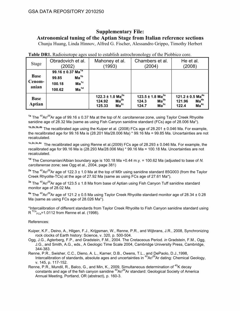
Table DR1. Radioisotope ages used to establish astrochronology of the Piobbico core.

StageObradovich et al.

(2002)Mahoney et al.

(1993)Chambers et al.

(2004)He et al.(2008)

BaseCenom-anian

99.16 ± 0.37 Ma1a

99.85 Ma1b

100.18 Ma1c

100.62 Ma1d

BaseAptian

122.3 ± 1.0 Ma2a

124.92 Ma2b

125.33 Ma2c

123.5 ± 1.8 Ma3a

124.3 Ma3b

124.7 Ma3c

121.2 ± 0.5 Ma4a

121.96 Ma4b

122.4 Ma4c

1a The 40Ar/39Ar age of 99.16 ± 0.37 Ma at the top of N. carcitanense zone, using Taylor Creek Rhyolitesanidine age of 28.32 Ma (same as using Fish Canyon sanidine standard (FCs) age of 28.006 Ma*).1b,2b,3b,4b The recalibrated age using the Kuiper et al. (2008) FCs age of 28.201 ± 0.046 Ma. For example,the recalibrated age for 99.16 Ma is (28.201 Ma/28.006 Ma) * 99.16 Ma = 99.85 Ma. Uncertainties are notrecalculated.1c,2c,3c,4c The recalibrated age using Renne et al.(2009) FCs age of 28.293 ± 0.046 Ma. For example, therecalibrated age for 99.16 Ma is (28.293 Ma/28.006 Ma) * 99.16 Ma = 100.18 Ma. Uncertainties are notrecalculated.1d The Cenomanian/Albian boundary age is 100.18 Ma +0.44 m.y. = 100.62 Ma (adjusted to base of N.carcitanense zone; see Ogg et al., 2004, page 381)2a The 40Ar/39Ar age of 122.3 ± 1.0 Ma at the top of M0r using sanidine standard 85G003 (from the TaylorCreek Rhyolite-TCs) at the age of 27.92 Ma (same as using FCs age of 27.61 Ma*).3a The 40Ar/39Ar age of 123.5 ± 1.8 Ma from base of Aptian using Fish Canyon Tuff sanidine standardmonitor age of 28.02 Ma.4a The 40Ar/39Ar age of 121.2 ± 0.5 Ma using Taylor Creek Rhyolite standard monitor age of 28.34 ± 0.28Ma (same as using FCs age of 28.026 Ma*).

*Intercalibration of different standards from Taylor Creek Rhyolite to Fish Canyon sanidine standard usingR TCs

FCs=1.0112 from Renne et al. (1998).

References:

Kuiper, K.F., Deino, A., Hilgen, F.J., Krijgsman, W., Renne, P.R., and Wijbrans, J.R., 2008, Synchronizingrock clocks of Earth history: Science, v. 320, p. 500-504.

Ogg, J.G., Agterberg, F.P., and Gradstein, F.M., 2004. The Cretaceous Period. in Gradstein, F.M., Ogg,J.G., and Smith, A.G., eds., A Geologic Time Scale 2004, Cambridge University Press, Cambridge,344-383.

Renne, P.R., Swisher, C.C., Dieno, A. L., Karner, D.B., Owens, T.L., and DePaolo, D.J.,1998,Intercalibration of standards, absolute ages and uncertainties in 40Ar/39Ar dating: Chemical Geology,v. 145, p. 117-152.

Renne, P.R., Mundil, R., Balco, G., and Min, K., 2009, Simultaneous determination of 40K decayconstants and age of the fish canyon sanidine 40Ar/39Ar standard: Geological Society of AmericaAnnual Meeting, Portland, OR (abstract), p. 160-3.

GSA DATA REPOSITORY 2010250

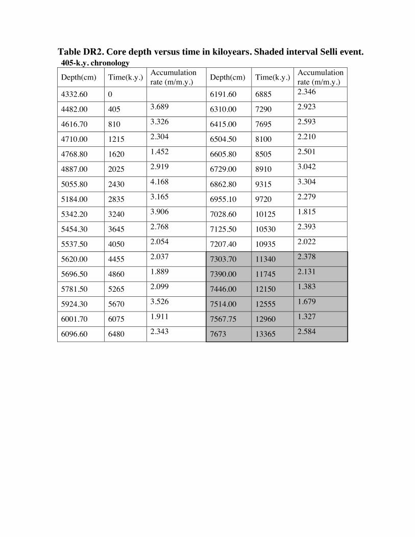
405-k.y. chronology

Depth(cm) Time(k.y.) Accumulationrate (m/m.y.) Depth(cm) Time(k.y.) Accumulation

rate (m/m.y.)4332.60 0 6191.60 6885 2.346

4482.00 405 3.689 6310.00 7290 2.923

4616.70 810 3.326 6415.00 7695 2.593

4710.00 1215 2.304 6504.50 8100 2.210

4768.80 1620 1.452 6605.80 8505 2.501

4887.00 2025 2.919 6729.00 8910 3.042

5055.80 2430 4.168 6862.80 9315 3.304

5184.00 2835 3.165 6955.10 9720 2.279

5342.20 3240 3.906 7028.60 10125 1.815

5454.30 3645 2.768 7125.50 10530 2.393

5537.50 4050 2.054 7207.40 10935 2.022

5620.00 4455 2.037 7303.70 11340 2.378

5696.50 4860 1.889 7390.00 11745 2.131

5781.50 5265 2.099 7446.00 12150 1.383

5924.30 5670 3.526 7514.00 12555 1.679

6001.70 6075 1.911 7567.75 12960 1.327

6096.60 6480 2.343 7673 13365 2.584

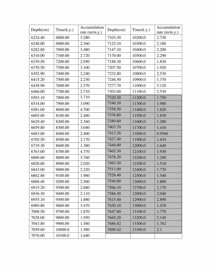
Table DR2. Core depth versus time in kiloyears. Shaded interval Selli event.

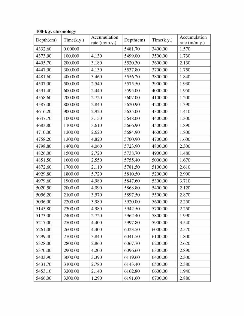
100-k.y. chronology

Depth(cm) Time(k.y.) Accumulationrate (m/m.y.) Depth(cm) Time(k.y.) Accumulation

rate (m/m.y.)4332.60 0.00000 5481.70 3400.00 1.5704373.90 100.000 4.130 5499.00 3500.00 1.7304405.70 200.000 3.180 5520.30 3600.00 2.1304447.00 300.000 4.130 5537.80 3700.00 1.7504481.60 400.000 3.460 5556.20 3800.00 1.8404507.00 500.000 2.540 5575.50 3900.00 1.9304531.40 600.000 2.440 5595.00 4000.00 1.9504558.60 700.000 2.720 5607.00 4100.00 1.2004587.00 800.000 2.840 5620.90 4200.00 1.3904616.20 900.000 2.920 5635.00 4300.00 1.4104647.70 1000.00 3.150 5648.00 4400.00 1.3004683.80 1100.00 3.610 5666.90 4500.00 1.8904710.00 1200.00 2.620 5684.90 4600.00 1.8004758.20 1300.00 4.820 5700.90 4700.00 1.6004798.80 1400.00 4.060 5723.90 4800.00 2.3004826.00 1500.00 2.720 5738.70 4900.00 1.4804851.50 1600.00 2.550 5755.40 5000.00 1.6704872.60 1700.00 2.110 5781.50 5100.00 2.6104929.80 1800.00 5.720 5810.50 5200.00 2.9004979.60 1900.00 4.980 5847.60 5300.00 3.7105020.50 2000.00 4.090 5868.80 5400.00 2.1205056.20 2100.00 3.570 5897.50 5500.00 2.8705096.00 2200.00 3.980 5920.00 5600.00 2.2505145.80 2300.00 4.980 5942.50 5700.00 2.2505173.00 2400.00 2.720 5962.40 5800.00 1.9905217.00 2500.00 4.400 5997.80 5900.00 3.5405261.00 2600.00 4.400 6023.50 6000.00 2.5705299.40 2700.00 3.840 6041.50 6100.00 1.8005328.00 2800.00 2.860 6067.70 6200.00 2.6205370.00 2900.00 4.200 6096.60 6300.00 2.8905403.90 3000.00 3.390 6119.60 6400.00 2.3005431.70 3100.00 2.780 6143.40 6500.00 2.3805453.10 3200.00 2.140 6162.80 6600.00 1.9405466.00 3300.00 1.290 6191.60 6700.00 2.880

Depth(cm) Time(k.y.) Accumulationrate (m/m.y.) Depth(cm) Time(k.y.) Accumulation

rate (m/m.y.)6224.40 6800.00 3.280 7103.30 10200.0 2.7306248.00 6900.00 2.360 7125.10 10300.0 2.1806282.80 7000.00 3.480 7147.10 10400.0 2.2006310.00 7100.00 2.720 7170.00 10500.0 2.2906339.50 7200.00 2.950 7188.30 10600.0 1.8306370.50 7300.00 3.100 7207.50 10700.0 1.9206392.90 7400.00 2.240 7232.80 10800.0 2.5306415.20 7500.00 2.230 7246.50 10900.0 1.3706438.90 7600.00 2.370 7277.70 11000.0 3.1206466.00 7700.00 2.710 7303.00 11100.0 2.5306503.10 7800.00 3.710 7320.50 11200.0 1.7506534.00 7900.00 3.090 7340.30 11300.0 1.9806581.00 8000.00 4.700 7358.50 11400.0 1.8206605.80 8100.00 2.480 7376.80 11500.0 1.8306629.40 8200.00 2.360 7389.60 11600.0 1.2806659.80 8300.00 3.040 7403.70 11700.0 1.4106683.80 8400.00 2.400 7413.26 11800.0 0.95606705.50 8500.00 2.170 7427.40 11900.0 1.6346719.30 8600.00 1.380 7446.00 12000.0 1.6406763.00 8700.00 4.370 7465.30 12100.0 1.9306800.60 8800.00 3.760 7478.20 12200.0 1.2906820.80 8900.00 2.020 7493.30 12300.0 1.5106843.00 9000.00 2.220 7511.00 12400.0 1.7706862.80 9100.00 1.980 7526.40 12500.0 1.5406888.40 9200.00 2.560 7546.80 12600.0 1.8006915.20 9300.00 2.680 7566.10 12700.0 2.1706936.30 9400.00 2.110 7586.50 12800.0 2.0406955.10 9500.00 1.880 7615.40 12900.0 2.8906989.80 9600.00 3.470 7630.10 13000.0 1.4707008.50 9700.00 1.870 7647.80 13100.0 1.7707028.00 9800.00 1.950 7669.20 13200.0 2.1407043.80 9900.00 1.580 7686.82 13300.0 1.7627059.60 10000.0 1.580 7699.42 13360.0 2.17076.00 10100.0 1.640

-40

0

40

7200 7300 7400 7500 7600

0

40

80

14 16 18 20 22 24 26 28 30

Ee

OP

Gre

ysca

leA

lbed

0

2 104

4 104

6 104

0 0.1 0.2 0.3 0.4

Pow

er

47 cm

6 cm

12 cm

3 cm

0

1000

2000

3000

0 0.05 0.1 0.15P

ower

14.7 cm

45 cm

8 cm

Frequency (cycles/cm)

E e

O

P

M0r

(A)

(B)

(C) (D)

Frequency (cycles/cm)

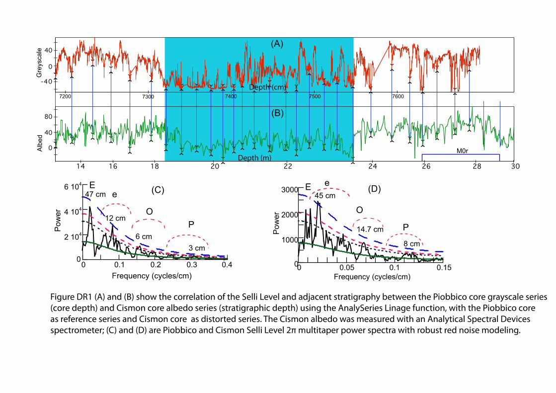
Figure DR1 (A) and (B) show the correlation of the Selli Level and adjacent stratigraphy between the Piobbico core grayscale series(core depth) and Cismon core albedo series (stratigraphic depth) using the AnalySeries Linage function, with the Piobbico core as reference series and Cismon core as distorted series. The Cismon albedo was measured with an Analytical Spectral Devices spectrometer; (C) and (D) are Piobbico and Cismon Selli Level 2π multitaper power spectra with robust red noise modeling.

Depth (m)

Depth (cm)

0 2 4 6 8 10 12 14Frequency (cycle/m)

0

2000

4000

Pow

er

19.2 20 20.8 21.6 22.4 23.2

01020304050607080

19.2 20 20.8 21.6 22.4 23.2

Mea

sure

d C

aCO

3 (%

)

0

500

1000

1500

2000 0 2 4 6 8 10 12 14

Pow

er

Depth (m)

(a)

(b)

(c)

(d)

1.4 m

0.46 m

0.084 m0.146 m

0.46 m

1.4 m

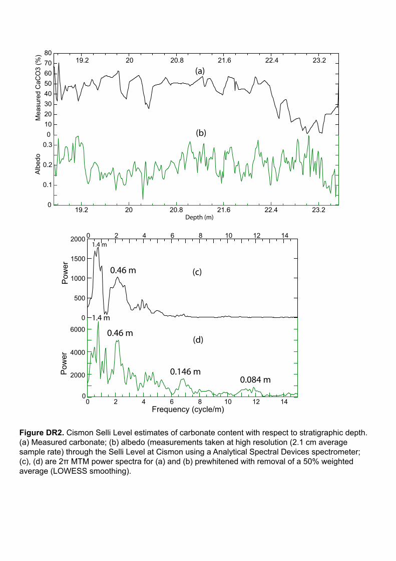
Figure DR2. Cismon Selli Level estimates of carbonate content with respect to stratigraphic depth. (a) Measured carbonate; (b) albedo (measurements taken at high resolution (2.1 cm average sample rate) through the Selli Level at Cismon using a Analytical Spectral Devices spectrometer; (c), (d) are 2π MTM power spectra for (a) and (b) prewhitened with removal of a 50% weighted average (LOWESS smoothing).

0

0.1

0.2

0.3

Alb

edo

6000

100

1000

104

105

0 0.1 0.2 0.3

PowerM90%95%99%

Pow

er

Frequency (cycles/cm)

148

36

4.64.3

400

20.6

12.5

7.27.7

3.84 3.6

16.9

80

9.8

E eccentricityObliquity

Precession

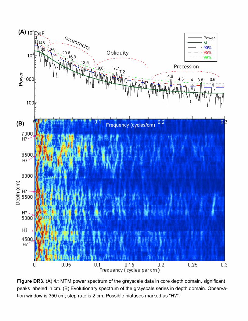
Figure DR3. (A) 4π MTM power spectrum of the grayscale data in core depth domain, significant peaks labeled in cm. (B) Evolutionary spectrum of the grayscale series in depth domain. Observa-tion window is 350 cm; step rate is 2 cm. Possible hiatuses marked as “H?”.

(A)

(B)

H?

H?

H?

H?

H?

H?

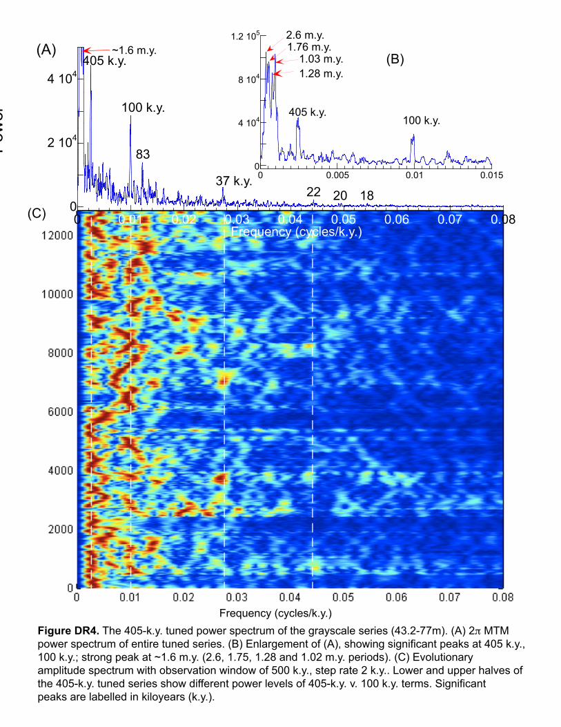
Figure DR4. The 405-k.y. tuned power spectrum of the grayscale series (43.2-77m). (A) 2π MTM power spectrum of entire tuned series. (B) Enlargement of (A), showing significant peaks at 405 k.y., 100 k.y.; strong peak at ~1.6 m.y. (2.6, 1.75, 1.28 and 1.02 m.y. periods). (C) Evolutionary amplitude spectrum with observation window of 500 k.y., step rate 2 k.y.. Lower and upper halves of the 405-k.y. tuned series show different power levels of 405-k.y. v. 100 k.y. terms. Significant peaks are labelled in kiloyears (k.y.).

(A)

(C)

(B)

0

4 104

8 104

1.2 105

0 0.005 0.01 0.015

1.28 m.y.

100 k.y.405 k.y.

1.03 m.y.1.76 m.y.2.6 m.y.

0

2 104

4 104

0 0.01 0.02 0.03 0.04 0.05 0.06 0.07 0.08

Pow

er

Frequency (cycles/k.y.)

~1.6 m.y.

100 k.y.

405 k.y.

37 k.y.22 20 18

83

Tim

e (k

.y.)

Frequency (cycles/k.y.)

0

4 104

8 104

0 0.01 0.02 0.03 0.04 0.05 0.06 0.07 0.08

Pow

er

Frequency (cycles/k.y.)

~1.6 m.y100 k.y.

405 k.y.

39 25 203322

0

4 104

8 104

1.2 105

0 0.005 0.01 0.015

1.28 m.y. 100 k.y.

405 k.y.

1.04 m.y.

2.13 m.y.2.6 m.y.

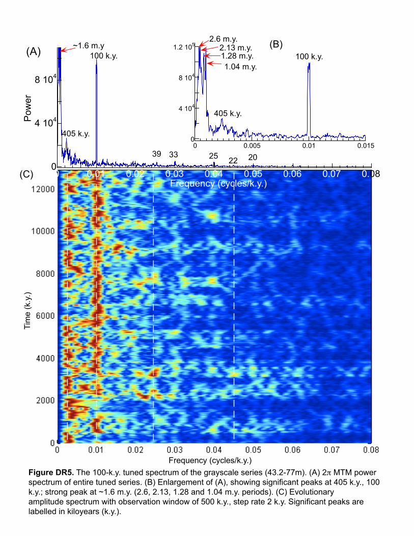
Figure DR5. The 100-k.y. tuned spectrum of the grayscale series (43.2-77m). (A) 2π MTM power spectrum of entire tuned series. (B) Enlargement of (A), showing significant peaks at 405 k.y., 100 k.y.; strong peak at ~1.6 m.y. (2.6, 2.13, 1.28 and 1.04 m.y. periods). (C) Evolutionary amplitude spectrum with observation window of 500 k.y., step rate 2 k.y. Significant peaks are labelled in kiloyears (k.y.).

(A)

(C)

(B)

Tim

e (k

.y.)

Frequency (cycles/k.y.)

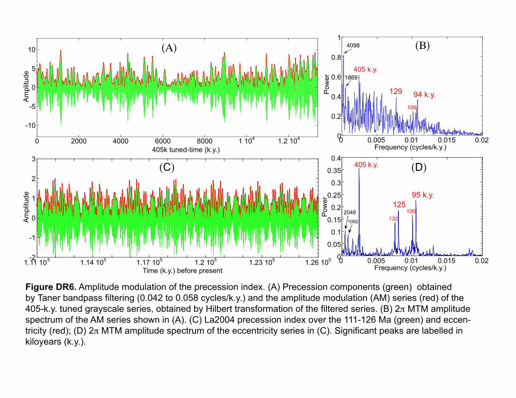
Figure DR6. Amplitude modulation of the precession index. (A) Precession components (green) obtained by Taner bandpass filtering (0.042 to 0.058 cycles/k.y.) and the amplitude modulation (AM) series (red) of the 405-k.y. tuned grayscale series, obtained by Hilbert transformation of the filtered series. (B) 2π MTM amplitude spectrum of the AM series shown in (A). (C) La2004 precession index over the 111-126 Ma (green) and eccen-tricity (red); (D) 2π MTM amplitude spectrum of the eccentricity series in (C). Significant peaks are labelled in kiloyears (k.y.).

(Α)

(D)

(Β)

(C)

0

0.2

0.4

0.6

0.8

1

0 0.005 0.01 0.015 0.02

Pow

er

Frequency (cycles/k.y.)

405 k.y.

94 k.y.129

1869

100

0

0.05

0.1

0.15

0.2

0.25

0.3

0.35

0.4

0 0.005 0.01 0.015 0.02

Pow

er

Frequency (cycles/k.y.)

405 k.y.

95 k.y.125

2048132

100

1092

-10

-5

0

5

10

0 2000 4000 6000 8000 1 104 1.2 104

Am

plitu

de

405k tuned-time (k.y.)

-2

-1

0

1

2

3

1.11 105 1.14 105 1.17 105 1.2 105 1.23 105 1.26 105

Am

plitu

de

Time (k.y.) before present

4098