Econometrica Supplementary Material

SUPPLEMENT TO “UNCERTAINTY SHOCKS IN A MODEL OFEFFECTIVE DEMAND”: TECHNICAL APPENDIX

(Econometrica, Vol. 85, No. 3, May 2017, 937–958)

BY SUSANTO BASU AND BRENT BUNDICK1

APPENDIX A: ADDITIONAL DETAILS CONCERNING EMPIRICAL EVIDENCE

A.1. Data Construction and Estimation

THIS SECTION PROVIDES additional details on the data construction and estimation proce-dure for the empirical evidence from Section 2 of the main text. We estimate our baselineVAR using data on the VXO, GDP, consumption, investment, hours worked, the GDP de-flator, the M2 money stock, and the Wu and Xia (2016) shadow rate. To match the conceptin the model, we measure consumption in the data as the sum of non-durable and servicesconsumption. Then, we use the sum of consumer durables and private fixed investmentas a measure of investment in our baseline empirical model. To match the quarterly fre-quency of the macroeconomic data, we average a weekly VXO series for each quarter.Thus, our measure of uncertainty captures the average implied stock market volatilitywithin a quarter. We convert output, consumption, investment, and hours worked to per-capita terms by dividing by population. Except for the shadow rate, all other variablesenter the VAR in log levels.

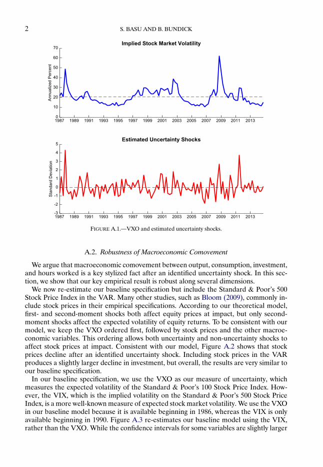
We include four lags in the estimation of the VAR and generate our confidence intervalsusing the Bayesian method outlined in Sims and Zha (1999).2 Figure A.1 plots the VXOover time as well as the series of identified, structural uncertainty shocks from the VAR.The empirical model identifies large uncertainty shocks after the 1987 stock market crash,the failure of Lehman Brothers, and the euro area sovereign debt crisis.

To generate the unconditional moments in Table II of the main text, we detrend the logof each empirical data series using the HP filter with a smoothing parameter of 1600. Wemeasure the unconditional volatility using the sample standard deviation of the detrendedvariable. We compute the empirical moments over the 1986–2014 sample period, whichis the same time frame used in our empirical VAR. In Appendix Section D.3, we providefurther analysis of the unconditional moments predicted by the model.

We estimate stochastic volatility using a simple model-free and nonparametric methodbased on rolling sample standard deviations. Given an empirical data series, we estimatea rolling 5-year standard deviation. This procedure provides a time-series of realizedvolatility estimates for the given data series. Then, we compute the standard deviationof this time-series of estimates. This simple measure provides an estimate of the stochas-tic volatility in the data series. If the actual data were homoscedastic, the estimates of the5-year rolling standard deviations should show little volatility and the resulting statisticwould be near zero.

1We thank Trenton Herriford for excellent research assistance. The replication package for this paper isavailable from the websites of Econometrica or the Federal Reserve Bank of Kansas City. The views expressedherein are solely those of the authors and do not necessarily reflect the views of the Federal Reserve Bank ofKansas City or the Federal Reserve System.

2We are grateful to A. Lee Smith for many helpful discussions and for sharing his code for computing theSims and Zha (1999) confidence intervals.

© 2017 The Econometric Society DOI: 10.3982/ECTA13960

2 S. BASU AND B. BUNDICK

FIGURE A.1.—VXO and estimated uncertainty shocks.

A.2. Robustness of Macroeconomic Comovement

We argue that macroeconomic comovement between output, consumption, investment,and hours worked is a key stylized fact after an identified uncertainty shock. In this sec-tion, we show that our key empirical result is robust along several dimensions.

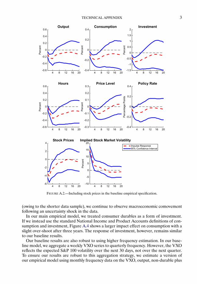
We now re-estimate our baseline specification but include the Standard & Poor’s 500Stock Price Index in the VAR. Many other studies, such as Bloom (2009), commonly in-clude stock prices in their empirical specifications. According to our theoretical model,first- and second-moment shocks both affect equity prices at impact, but only second-moment shocks affect the expected volatility of equity returns. To be consistent with ourmodel, we keep the VXO ordered first, followed by stock prices and the other macroe-conomic variables. This ordering allows both uncertainty and non-uncertainty shocks toaffect stock prices at impact. Consistent with our model, Figure A.2 shows that stockprices decline after an identified uncertainty shock. Including stock prices in the VARproduces a slightly larger decline in investment, but overall, the results are very similar toour baseline specification.

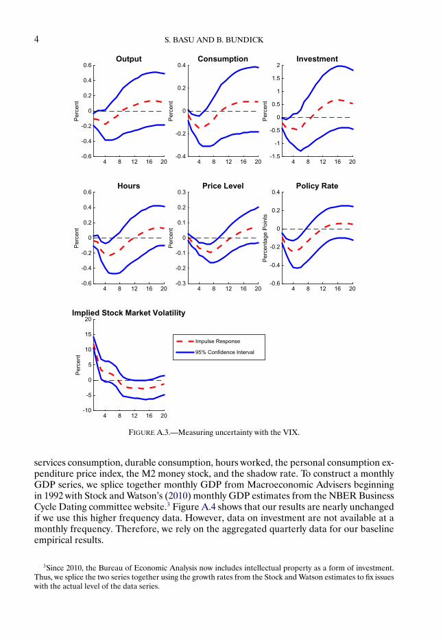
In our baseline specification, we use the VXO as our measure of uncertainty, whichmeasures the expected volatility of the Standard & Poor’s 100 Stock Price Index. How-ever, the VIX, which is the implied volatility on the Standard & Poor’s 500 Stock PriceIndex, is a more well-known measure of expected stock market volatility. We use the VXOin our baseline model because it is available beginning in 1986, whereas the VIX is onlyavailable beginning in 1990. Figure A.3 re-estimates our baseline model using the VIX,rather than the VXO. While the confidence intervals for some variables are slightly larger

TECHNICAL APPENDIX 3

FIGURE A.2.—Including stock prices in the baseline empirical specification.

(owing to the shorter data sample), we continue to observe macroeconomic comovementfollowing an uncertainty shock in the data.

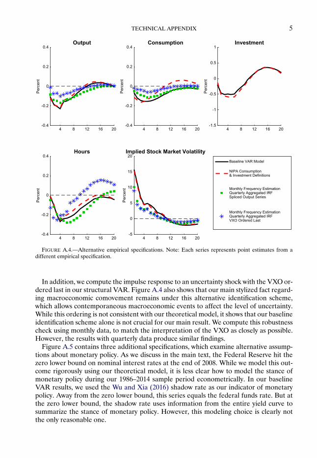
In our main empirical model, we treated consumer durables as a form of investment.If we instead use the standard National Income and Product Accounts definitions of con-sumption and investment, Figure A.4 shows a larger impact effect on consumption with aslight over-shoot after three years. The response of investment, however, remains similarto our baseline results.

Our baseline results are also robust to using higher frequency estimation. In our base-line model, we aggregate a weekly VXO series to quarterly frequency. However, the VXOreflects the expected S&P 100 volatility over the next 30 days, not over the next quarter.To ensure our results are robust to this aggregation strategy, we estimate a version ofour empirical model using monthly frequency data on the VXO, output, non-durable plus

4 S. BASU AND B. BUNDICK

FIGURE A.3.—Measuring uncertainty with the VIX.

services consumption, durable consumption, hours worked, the personal consumption ex-penditure price index, the M2 money stock, and the shadow rate. To construct a monthlyGDP series, we splice together monthly GDP from Macroeconomic Advisers beginningin 1992 with Stock and Watson’s (2010) monthly GDP estimates from the NBER BusinessCycle Dating committee website.3 Figure A.4 shows that our results are nearly unchangedif we use this higher frequency data. However, data on investment are not available at amonthly frequency. Therefore, we rely on the aggregated quarterly data for our baselineempirical results.

3Since 2010, the Bureau of Economic Analysis now includes intellectual property as a form of investment.Thus, we splice the two series together using the growth rates from the Stock and Watson estimates to fix issueswith the actual level of the data series.

TECHNICAL APPENDIX 5

FIGURE A.4.—Alternative empirical specifications. Note: Each series represents point estimates from adifferent empirical specification.

In addition, we compute the impulse response to an uncertainty shock with the VXO or-dered last in our structural VAR. Figure A.4 also shows that our main stylized fact regard-ing macroeconomic comovement remains under this alternative identification scheme,which allows contemporaneous macroeconomic events to affect the level of uncertainty.While this ordering is not consistent with our theoretical model, it shows that our baselineidentification scheme alone is not crucial for our main result. We compute this robustnesscheck using monthly data, to match the interpretation of the VXO as closely as possible.However, the results with quarterly data produce similar findings.

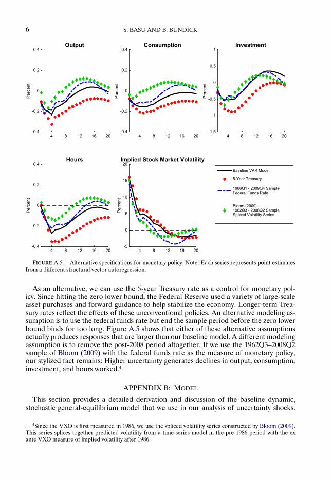
Figure A.5 contains three additional specifications, which examine alternative assump-tions about monetary policy. As we discuss in the main text, the Federal Reserve hit thezero lower bound on nominal interest rates at the end of 2008. While we model this out-come rigorously using our theoretical model, it is less clear how to model the stance ofmonetary policy during our 1986–2014 sample period econometrically. In our baselineVAR results, we used the Wu and Xia (2016) shadow rate as our indicator of monetarypolicy. Away from the zero lower bound, this series equals the federal funds rate. But atthe zero lower bound, the shadow rate uses information from the entire yield curve tosummarize the stance of monetary policy. However, this modeling choice is clearly notthe only reasonable one.

6 S. BASU AND B. BUNDICK

FIGURE A.5.—Alternative specifications for monetary policy. Note: Each series represents point estimatesfrom a different structural vector autoregression.

As an alternative, we can use the 5-year Treasury rate as a control for monetary pol-icy. Since hitting the zero lower bound, the Federal Reserve used a variety of large-scaleasset purchases and forward guidance to help stabilize the economy. Longer-term Trea-sury rates reflect the effects of these unconventional policies. An alternative modeling as-sumption is to use the federal funds rate but end the sample period before the zero lowerbound binds for too long. Figure A.5 shows that either of these alternative assumptionsactually produces responses that are larger than our baseline model. A different modelingassumption is to remove the post-2008 period altogether. If we use the 1962Q3–2008Q2sample of Bloom (2009) with the federal funds rate as the measure of monetary policy,our stylized fact remains: Higher uncertainty generates declines in output, consumption,investment, and hours worked.4

APPENDIX B: MODEL

This section provides a detailed derivation and discussion of the baseline dynamic,stochastic general-equilibrium model that we use in our analysis of uncertainty shocks.

4Since the VXO is first measured in 1986, we use the spliced volatility series constructed by Bloom (2009).This series splices together predicted volatility from a time-series model in the pre-1986 period with the exante VXO measure of implied volatility after 1986.

TECHNICAL APPENDIX 7

The baseline model shares many features of the models of Ireland (2003), Ireland (2011),and Jermann (1998). The model features optimizing households and firms and a centralbank that follows a Taylor rule to stabilize inflation and offset adverse shocks. We allowfor sticky prices using the quadratic-adjustment costs specification of Rotemberg (1982).Our baseline model considers technology and household discount rate shocks. The dis-count rate shocks have a time-varying second moment, which we interpret as the degreeof uncertainty about future demand.

B.1. Households

In our model, the representative household maximizes lifetime utility given Epstein–Zin preferences over streams of consumption Ct and leisure 1 −Nt . The key parametersgoverning household decisions are its risk aversion σ over the consumption-leisure basketand its intertemporal elasticity of substitution ψ. The parameter θV � (1 −σ)(1 − 1/ψ)−1

controls the household’s preference for the resolution of uncertainty. The household re-ceives labor income Wt for each unit of labor Nt supplied to the representative inter-mediate goods-producing firm. The representative household also owns the intermediategoods firm and holds equity shares St and one-period risk-less bonds Bt issued by repre-sentative intermediate goods firm. Equity shares have a price of PEt and pay dividendsDE

t

for each share St owned. The risk-less bonds return the gross one-period risk-free inter-est rate RRt . The household divides its income from labor and its financial assets betweenconsumption Ct and holdings of financial assets St+1 and Bt+1 to carry into next period.The discount rate of the household β is subject to shocks via the stochastic process at .

The representative household maximizes lifetime utility by choosing Ct+s�Nt+s, Bt+s+1,and St+s+1 for all s = 0�1�2� � � � by solving the following problem:

Vt = max[at

(Cηt (1 −Nt)

1−η)(1−σ)/θV +β(EtV

1−σt+1

)1/θV ]θV /(1−σ)

subject to its intertemporal household budget constraint each period,

Ct + PEtPtSt+1 + 1

RRtBt+1 ≤ Wt

PtNt +

(DEt

Pt+ PEtPt

)St +Bt�

Using a Lagrangian approach, household optimization implies the following first-orderconditions:

∂Vt

∂Ct= λt� (S.1)

∂Vt

∂Nt

= λt Wt

Pt� (S.2)

PEtPt

= Et

{(λt+1

λt

)(DEt+1

Pt+1+ PEt+1

Pt+1

)}� (S.3)

1 =RRt Et{(λt+1

λt

)}� (S.4)

8 S. BASU AND B. BUNDICK

where λt denotes the Lagrange multiplier on the household budget constraint. Epstein–Zin preferences imply the following relationships:

∂Vt

∂Ct= atV

1−(1−σ)/θVt η

(Cηt (1 −Nt)

1−η)(1−σ)/θV

Ct�

∂Vt+1

∂Ct+1= at+1V

1−(1−σ)/θVt+1 η

(Cηt+1(1 −Nt+1)

1−η)(1−σ)/θV

Ct+1�

∂Vt

∂Ct+1= βV

1−(1−σ)/θVt

(EtV

1−σt+1

)1/θV −1Et

{V −σt+1

(∂Vt+1

∂Ct+1

)}

= βV1−(1−σ)/θVt

(EtV

1−σt+1

)1/θV −1Et

{V −σt+1 at+1V

1−(1−σ)/θVt+1 η

(Cηt+1(1 −Nt+1)

1−η)(1−σ)/θV

Ct+1

}�

Thus, we define the household stochastic discount factor M between periods t and t + 1:

Mt+1 �(∂Vt/∂Ct+1

∂Vt/∂Ct

)=

(βat+1

at

)(Cηt+1(1 −Nt+1)

1−η

Cηt (1 −Nt)

1−η

)(1−σ)/θV ( Ct

Ct+1

)(V 1−σt+1

Et

[V 1−σt+1

])1−1/θV

�

Using the stochastic discount factor, we can eliminate λ and simplify Equations (S.1)–(S.4):

1 −ηη

Ct

1 −Nt

= Wt

Pt� (S.5)

PEtPt

= Et

{Mt+1

(DEt+1

Pt+1+ PEt+1

Pt+1

)}� (S.6)

1 =RRt Et{Mt+1}� (S.7)

Equation (S.5) represents the household intratemporal optimality condition with respectto consumption and leisure, and Equations (S.6) and (S.7) represent the Euler equationsfor equity shares and one-period risk-less firm bonds.

B.2. Intermediate Goods Producers

Each intermediate goods-producing firm i rents labor Nt(i) from the representativehousehold to produce intermediate good Yt(i). Intermediate goods are produced in amonopolistically competitive market where producers face a quadratic cost of changingtheir nominal price Pt(i) each period. The intermediate goods firms own their capitalstocks Kt(i), and face convex costs of changing the quantity of installed capital. Firmsalso choose the rate of utilization of their installed physical capital Ut(i), which affectsits depreciation rate. Each firm issues equity shares St(i) and one-period risk-less bondsBt(i). Firm i chooses Nt(i), It(i), Ut(i), and Pt(i) to maximize firm cash flows Dt(i)/Pt(i)given aggregate demand Yt and price Pt of the finished goods sector. The intermediategoods firms all have the same constant returns to scale Cobb–Douglas production func-tion, subject to a fixed cost of production � and their level of productivity Zt .

TECHNICAL APPENDIX 9

Each firm producing intermediate goods maximizes discounted cash flows using thehousehold’s stochastic discount factor:

maxEt∞∑s=0

(∂Vt/∂Ct+s∂Vt/∂Ct

)[Dt+s(i)Pt+s

]

subject to the production function:

[Pt(i)

Pt

]−θμYt ≤

[Kt(i)Ut(i)

]α[ZtNt(i)

]1−α −��

and subject to the capital accumulation equation:

Kt+1(i)=(

1 − δ(Ut(i)) − φK

2

(It(i)

Kt(i)− δ

)2)Kt(i)+ It(i)�

where

Dt(i)

Pt=

[Pt(i)

Pt

]1−θμYt − Wt

PtNt(i)− It(i)− φP

2

[Pt(i)

ΠPt−1(i)− 1

]2

Yt

and depreciation depends on utilization via the following functional form:

δ(Ut(i)

) = δ+ δ1

(Ut(i)−U) +

(δ2

2

)(Ut(i)−U)2

�

The behavior of each firm i satisfies the following first-order conditions:

Wt

PtNt(i)= (1 − α)Ξt

[Kt(i)Ut(i)

]α[ZtNt(i)

]1−α�

RKtPtUt(i)Kt(i)= αΞt

[Kt(i)Ut(i)

]α[ZtNt(i)

]1−α�

qtδ′(Ut(i)

)Ut(i)Kt(i)= αΞt

[Kt(i)Ut(i)

]α[ZtNt(i)

]1−α�

φP

[Pt(i)

ΠPt−1(i)− 1

][Pt

ΠPt−1(i)

]

= (1 − θμ)[Pt(i)

Pt

]−θμ+ θμΞt

[Pt(i)

Pt

]−θμ−1

+φPEt{Mt+1

Yt+1

Yt

[Pt+1(i)

ΠPt(i)− 1

][Pt+1(i)

ΠPt(i)

Pt

Pt(i)

]}�

(S.8)

qt = Et

{Mt+1

(Ut+1(i)

RKt+1

Pt+1+ qt+1

(1 − δ(Ut+1(i)

) − φK

2

(It+1(i)

Kt+1(i)− δ

)2

+φK(It+1(i)

Kt+1(i)− δ

)(It+1(i)

Kt+1(i)

)))}�

10 S. BASU AND B. BUNDICK

1qt

= 1 −φK(It(i)

Kt(i)− δ

)�

where Ξt is the marginal cost of producing one additional unit of intermediate good i,and qt is the price of a marginal unit of installed capital. RKt /Pt is the marginal revenueproduct per unit of capital services KtUt , which is paid to the owners of the capital stock.Our adjustment cost specification is similar to the specification used by Jermann (1998)and allows Tobin’s q to vary over time.

Each intermediate goods firm finances a percentage ν of its capital stock each periodwith one-period risk-less bonds. The bonds pay the one-period real risk-free interest rate.Thus, the quantity of bonds Bt(i) = νKt(i). Total firm cash flows are divided betweenpayments to bond holders and equity holders as follows:

DEt (i)

Pt= Dt(i)

Pt− ν

(Kt(i)− 1

RRtKt+1(i)

)�

Since the Modigliani and Miller (1958) theorem holds in our model, leverage does notaffect firm value or optimal firm decisions. Leverage makes the payouts and price of eq-uity more volatile and allows us to define a concept of equity returns in the model. Weuse the volatility of equity returns implied by the model to calibrate our uncertainty shockprocesses in Section 6.

B.3. Final Goods Producers

The representative final goods producer uses Yt(i) units of each intermediate goodproduced by the intermediate goods-producing firm i ∈ [0�1]. The intermediate output istransformed into final output Yt using the following constant returns to scale technology:

[∫ 1

0Yt(i)

(θμ−1)/θμ di

]θμ/(θμ−1)

≥ Yt�

Each intermediate good Yt(i) sells at nominal price Pt(i) and each final good sells atnominal price Pt . The finished goods producer chooses Yt and Yt(i) for all i ∈ [0�1] tomaximize the following expression of firm profits:

PtYt −∫ 1

0Pt(i)Yt(i)di�

subject to the constant returns to scale production function. Finished goods-produceroptimization results in the following first-order condition:

Yt(i)=[Pt(i)

Pt

]−θμYt�

The market for final goods is perfectly competitive, and thus the final goods-producingfirm earns zero profits in equilibrium. Using the zero-profit condition, the first-order con-dition for profit maximization, and the firm objective function, the aggregate price indexPt can be written as follows:

Pt =[∫ 1

0Pt(i)

1−θμ di]1/(1−θμ)

�

TECHNICAL APPENDIX 11

B.4. Equilibrium

The assumption of Rotemberg (1982) (as opposed to Calvo (1983)) pricing impliesthat we can model our production sector as a single representative intermediate goods-producing firm. In the symmetric equilibrium, all intermediate goods firms choose thesame price Pt(i)= Pt , employ the same amount of labor Nt(i)=Nt , and choose the samelevel of capital and utilization rate Kt(i) = Kt and Ut(i) = Ut . Thus, all firms have thesame cash flows and payout structure between bonds and equity. With a representativefirm, we can define the unique markup of price over marginal cost as μt = 1/Ξt and grossinflation as Πt = Pt/Pt−1.

B.5. Monetary Policy

We assume a cashless economy where the monetary authority sets the net nominal in-terest rate rt to stabilize inflation and output growth. Monetary policy adjusts the nominalinterest rate in accordance with the following rule:

rt = r + ρπ(πt −π)+ ρy�yt� (S.9)

where rt = ln(Rt), πt = ln(Πt) , and �yt = ln(Yt/Yt−1). Changes in the nominal interestrate affect expected inflation and the real interest rate. Thus, we include the followingEuler equation for a zero net supply nominal bond in our equilibrium conditions:

1 =RtEt{Mt+1

(1Πt+1

)}� (S.10)

B.6. Shock Processes

The demand and technology shock processes are parameterized as follows:

at = (1 − ρa)a+ ρaat−1 + σat−1εat �

σat = (1 − ρσa)σa + ρσaσat−1 + σσaεσat �Zt = (1 − ρZ)Z + ρZZt−1 + σZεZt �

εat and εZt are first-moment shocks that capture innovations to the level of the stochasticprocess for technology and household discount factors. We refer to εσat as second-momentor “uncertainty” shock since it captures innovations to the volatility of the exogenousprocess for household discount factors. An increase in the volatility of the shock processincreases the uncertainty about the future time path of household demand. All threestochastic shocks are independent, standard normal random variables.

B.7. Solution Method

Our primary focus is examining the effect of an increase in the second moment ofthe preference shock process. Using a standard first-order or log-linear approximation tothe equilibrium conditions of our model would not allow us to examine second-momentshocks, since the approximated policy functions are invariant to the volatility of the shockprocesses. Similarly, second-moment shocks would only enter as cross-products with theother state variables in a second-order approximation, and thus we could not study the

12 S. BASU AND B. BUNDICK

effects of shocks to the second moments alone. In a third-order approximation, however,second-moment shocks enter independently in the approximated policy functions. Thus, athird-order approximation allows us to compute an impulse response to an increase in thevolatility of the discount rate shocks, while holding constant the levels of those variables.

To solve the baseline model, we use the Dynare software package developed byAdjemian, Bastani, Juillard, Karamé, Mihoubi, Perendia, Pfeifer, Ratto, and Villemot(2011). Dynare computes the rational expectations solution to the model using third-order Taylor series approximation around the deterministic steady state of the model.Section B.8 contains all the equilibrium conditions for the baseline model. To assist in nu-merically calibrating and solving the model, we introduce constants into the period utilityfunction and the production function to normalize the value function V and output Yto both equal 1 at the deterministic steady state. We use Dynare version 4.4.3 in Matlab2014b to solve and simulate the baseline model.

As discussed in Fernández-Villaverde, Guerrón-Quintana, Rubio-Ramírez, and Uribe(2011), approximations higher than first-order move the ergodic distributions of themodel endogenous variables away from their deterministic steady-state values. With theexception of our simulation exercises in Sections 5.3 and 6.2 of the main text, we alwaysanalyze a traditional impulse response in percent deviation from the stochastic steadystate of the model. To construct these responses, we set the exogenous shocks in the modelto zero and iterate our third-order solution forward. After a sufficient number of periods,the endogenous variables of the model converge to a fixed point, which we denote thestochastic steady state. We then hit the economy with a one standard deviation uncer-tainty shock but assume the economy is hit by no further shocks. We compute the impulseresponse as the percent deviation between the equilibrium responses and the pre-shockstochastic steady state.

By default, Dynare uses an alternative simulation-based procedure to construct im-pulse responses for second-order and higher model solutions. This method is based onthe generalized impulse response of Koop, Pesaran, and Potter (1996). As opposed to be-ing centered around the stochastic steady state, these alternative responses are computedin deviations from the ergodic mean of the endogenous variables. In addition, these re-sponses combine both the effects of higher uncertainty about future shocks with higherrealized volatility of the actual shocks hitting the economy. We choose to compute the tra-ditional impulse responses at the stochastic steady state for two reasons. First, Figure B.1shows that these two procedures produce nearly identical results, yet the computationaltime is significantly less for the traditional impulse response. This computational advan-tage is particularly helpful when we estimate some of the model parameters using impulseresponse matching, which requires us to repeatedly solve the model under various param-eterizations. Second, the traditional impulse response around the stochastic steady stateallows us to analyze an increase in uncertainty about the future without any change in therealized volatility of the shock processes.

B.8. Complete Model

In the symmetric equilibrium, the baseline model in Dynare notation is as follows:

y + fixedcost = productionconstant*(z*n)^(1 - alpha)

*(u*k(-1))^(alpha);

c + leverageratio*k/rr = w*n + de + leverageratio*k(-1);

TECHNICAL APPENDIX 13

FIGURE B.1.—Alternative impulse response construction. Note: Impulse responses are plotted in percentdeviations from either the stochastic steady state or their ergodic mean.

w = ((1 - eta)/eta)*c/(1 - l);

vf = (utilityconstant*a*(c^(eta)*(1 - n)^(1 - eta))^((1- sigma)/thetavf)+ beta*expvfsigma^(1/thetavf))^(thetavf/(1 - sigma));

expvfsigma = vf(+1)^(1 - sigma);

w*n = (1 - alpha)*(y + fixedcost)/mu;

rrk*u*k(-1) = alpha*(y + fixedcost)/mu;

q*deltauprime*u*k(-1) = alpha*(y + fixedcost)/mu;

k = ((1 - deltau) - (phik/2)*(inv/k(-1) - delta0)^(2))*k(-1)+ inv;

deltau = delta0 + delta1*(u-1) + (delta2/2)*(u-1)^(2);

14 S. BASU AND B. BUNDICK

deltauprime = delta1 + delta2*(u-1);

sdf = beta*(a/a(-1))

*((c^(eta)*(1 - n)^(1 - eta))/(c(-1)^(eta)*(1 - n(-1))^(1 - eta)))^((1 - sigma)/thetavf)

*(c(-1)/c)*(vf^(1 - sigma)/expvfsigma(-1))^(1 -1/thetavf);

1 = rr*sdf(+1);

1 = r*sdf(+1)*(pie(+1))^(-1);

1 = sdf(+1)*(de(+1) + pe(+1))/pe;

log(r) = rhor*log(r(-1))+ (1 - rhor)*(log(rss) + rhopie*log(pie/piess)+ rhoy*log(y/y(-1)));

de = y - w*n - inv - (phip/2)*(pie/piess - 1)^(2)*y- leverageratio*(k(-1) - k/rr);

1 = sdf(+1)*(u(+1)*rrk(+1)+ q(+1)*((1 - deltau(+1)) - (phik/2)*(inv(+1)/k- delta0)^(2)+ phik*(inv(+1)/k - delta0)*(inv(+1)/k)))/q;

1/q = 1 - phik*(inv/k(-1) - delta0);

phip*(pie/piess - 1)*(pie/piess)= (1 - thetamu) + thetamu/mu

+ sdf(+1)*phip*(pie(+1)/piess - 1)*(y(+1)/y)

*(pie(+1)/piess);

expre = (de(+1) + pe(+1))/pe;

expre2 = (de(+1) + pe(+1))^(2)/pe^(2);

varexpre = expre2 - (expre)^(2);

a = (1 - rhoa)*ass + rhoa*a(-1) + vola(-1)*ea;

vola = rhovola*vola(-1) + (1 - rhovola)*volass + volvola*evola;

z = (1 - rhoz)*zss + rhoz*z(-1) + volzss*ez;

Since the capital stock is predetermined, we lag the capital stockK variables by one periodrelative to the timing in the model derivation.

TECHNICAL APPENDIX 15

APPENDIX C: ESTIMATING VARS ON SIMULATED MODEL DATA

This section provides additional details on our simulation exercises from Sections 5.3and 6.2 of the main text. After a burn-in sample, we simulate 30 years of data fromour theoretical model. We then estimate our baseline empirical VAR, described in Ap-pendix A.1, using the simulated model data. In Section 5.3, the variables in the VAR arethe model-implied VXO, output, consumption, investment, hours worked, the price level,and the short-term nominal policy rate. All variables, except the policy interest rate, en-ter the VAR in log levels. To match our empirical specification, we use the annualized,net nominal interest rate as our measure of monetary policy. After estimating the VAR,we compute the impulse responses to an identified uncertainty shock using a Choleskydecomposition with the VXO ordered first. We then repeat this exercise 10,000 times,which provides us with the probability distribution of the impulse response function. InSection 6.2, we also add in the log of the model-implied markup μt after the policy rate.

Since we compute a third-order approximation for this exercise, rather than a full non-linear solution, the simulated variance for the model-implied stock market can occasion-ally go negative. To reproduce our empirical framework where the VXO is always positive,we truncate simulated values for the VXO at a lower bound of 1 percent, which impliesthat the log VXO always remains positive. Since the estimated impulse responses reflectthe average effect of uncertainty on the economy, we plot the unconditional generalizedimpulse responses as the true model responses in Figures 5 and 6 of the main text.

APPENDIX D: EXAMINING MODEL FEATURES AND PREDICTIONS

Our baseline model is consistent with both the qualitative comovement and quantitativepredictions of an identified uncertainty shock in the data. In the following sections, weprovide further details on the key model ingredients and further examine some additionalpredictions of the model.

D.1. Countercyclical Markups in a Real Model

Our mechanism for generating macroeconomic comovement relies on countercyclicalmarkups following an uncertainty shock. Following much of the literature, we implementcountercyclical markups by assuming prices adjust slowly to changing economic condi-tions. However, our main results are unchanged if we instead consider a model with coun-tercyclical markups but without nominal rigidities. To illustrate this idea, we replace ourNew Keynesian Phillips Curve in Appendix Equation (S.8) with the following equation:

log(μt/μ)= εμy log(Yt/Y)� (S.11)

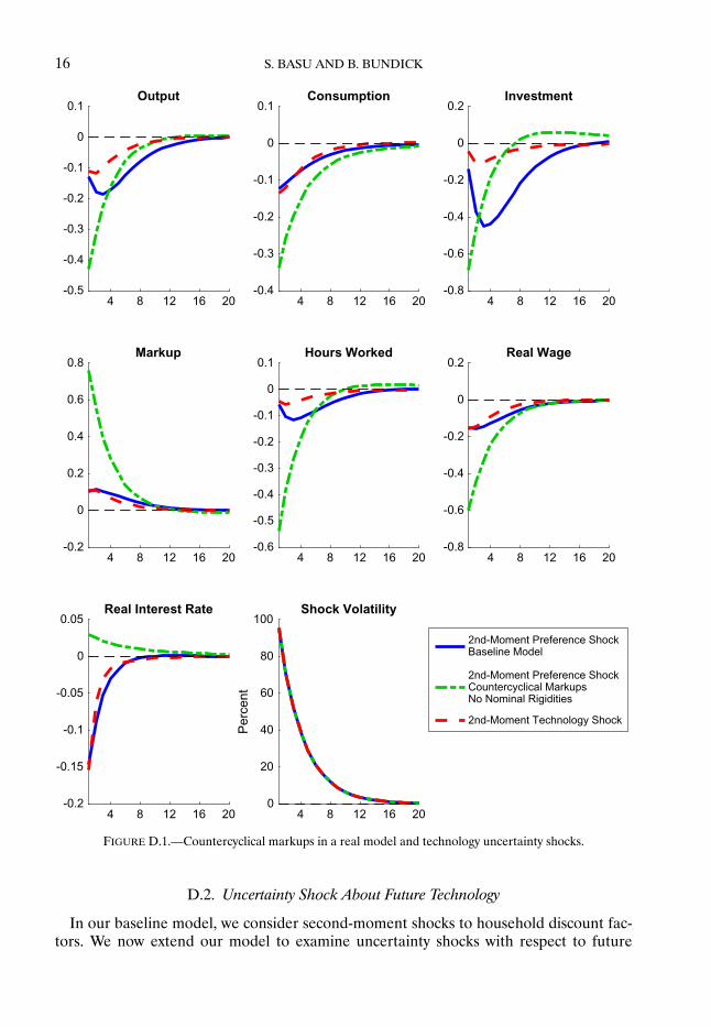
where μt is the markup over marginal cost and Yt is output. εμy denotes the elasticityof the markup with respect to output. The variables without t-subscripts denote theirsteady-state values. Following the empirical evidence of Bils, Klenow, and Malin (2014),we calibrate εμy = −1�8. Figure D.1 plots the impulse responses to a demand uncertaintyshock in this entirely real model with countercyclical markups. Even without nominalrigidities, countercyclical markups can generate macroeconomic comovment in responseto an uncertainty shock.

16 S. BASU AND B. BUNDICK

FIGURE D.1.—Countercyclical markups in a real model and technology uncertainty shocks.

D.2. Uncertainty Shock About Future Technology

In our baseline model, we consider second-moment shocks to household discount fac-tors. We now extend our model to examine uncertainty shocks with respect to future

TECHNICAL APPENDIX 17

technology. We replace our stochastic process for technology with the following two equa-tions:

Zt = (1 − ρZ)Z + ρZZt−1 + σZt−1εZt �

σZt = (1 − ρσZ)σZ + ρσZσZt−1 + σσZεσZt �Figure D.1 shows the impulse responses to a technology uncertainty shock.5 Similarly toa demand uncertainty shock, higher uncertainty about future technology can generate adecline in output, consumption, investment, and hours worked.

However, there are two reasons why second-moment technology shocks are not asgood at matching the quantitative aspects of the economy’s response to an uncertaintyshock. First, technology uncertainty shocks require significantly larger shocks to producesignificant fluctuations in output and its components. To produce the outcomes in Fig-ure D.1, we needed a five-fold increase in the volatility of the technology shocks relativeto our baseline calibration. This more volatile shock process implies too much uncon-ditional and stochastic volatility in key macroeconomic aggregates. Second, conditionalon a given movement in consumption, a technology impulse response generates a muchsmaller movement in investment than a demand uncertainty shock. When the uncer-tainty about future technology increases, higher capital provides a hedge against possi-ble negative shocks to future marginal costs. This additional substitution effect, which isnot present under a demand uncertainty shock, provides an incentive for a firm to avoiddisinvesting in the capital stock when uncertainty about future technology increases. Ac-cordingly, investment falls by only 10 basis points after a technology uncertainty shock butfalls by over 50 basis points after a demand uncertainty shock. Since capital and labor arecomplements in production, the time path of investment implies that equilibrium hoursworked also falls by less after a technology uncertainty shock.

D.3. Model-Implied Unconditional Moments

Building on the discussion in Section 5.2 of the main text, we now provide furthercomparison of the unconditional moments generated by our model with their empiricalcounterparts. Given that uncertainty shocks generate stochastic volatility in key macroe-conomic aggregates, a key litmus test for our model will be its ability to match the time-varying volatility in the data.

To evaluate the model’s fit, we compare its simulated moments with their data coun-terparts along three dimensions. First, we assess the model’s ability to match the uncon-ditional volatility in the data as measured by the sample standard deviation. Second, weevaluate the amount of stochastic volatility in key macro aggregates both in the data andin the model. Finally, we examine the average real interest rate, equity premium, andimplied stock market volatility generated by the model. We examine the model’s pre-dictions for output, consumption, investment, hours worked, the real interest rate, equitypremium, and the implied stock market volatility. For output and its components, we con-struct the data as outlined in Appendix A.1. For the real interest rate and equity premium,we calculate the quarterly, annualized ex post returns.6

5For this exercise, we calibrate σZ = 0�0064 and σσZ = 0�0061. This calibration implies a 95% increase inthe volatility of future technology shocks, which is similar to our baseline model using demand shocks. We alsoslightly increase the investment adjustment costs (φK = 10) to generate a larger decline in investment.

6We calculate the real interest rate by subtracting the ex post GDP deflator inflation rate from the effectivefederal funds rate.

18 S. BASU AND B. BUNDICK

To compare the distance between the model-implied moments and their empiri-cal counterparts, we generate small-sample bootstrapped probability intervals from themodel. Our empirical moments come from about a 30-year sample of quarterly data.We want to determine the likelihood that the moments from this given 30-year sampleof data could be generated by our baseline model. To compute the probability intervalfor each moment, we simulate the model economy for 30 years after an initial burn-inperiod. Then, we compute and save all the desired model-implied moments using thissmall sample of simulated data. We repeat this exercise 10,000 times, which provides uswith a series of small-sample estimates for each moment of interest. Table D.I reportsthe mean and the 95% probability interval for each model-implied moment as well astheir empirical counterparts. If the empirical moment falls outside of this model-impliedprobability interval, it is highly statistically unlikely that the model is able to generate mo-ments consistent with the data. In Table II of the main text, we report the mean for eachmodel-implied moment.

Our model is generally consistent with the unconditional and stochastic volatility inoutput, consumption, and investment. For each of these variables, the empirical momentfalls within the small-sample probability interval generated by the model. The model doesstruggle slightly in generating sufficient unconditional and stochastic volatility in hoursworked. However, the general fit of the model suggests that we would likely draw similarconclusions about the effects of uncertainty shocks if we instead chose to calibrate ourmodel directly using the stochastic volatility in key macro variables (as opposed to ourimpulse response matching procedure).

However, the model’s predictions for the real interest rate, equity premium, and im-plied stock market volatility could be improved. On average, the model generates realinterest rates that are too high relative to the data. In addition, the average equity pre-mium and VXO in the model are lower than in the data. Finally, the model does notgenerate enough volatility in the real interest rate, equity premium, or implied stock mar-ket volatility.

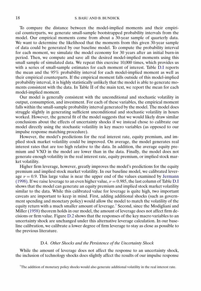
Higher firm leverage, however, greatly improves the model’s predictions for the equitypremium and implied stock market volatility. In our baseline model, we calibrated lever-age ν = 0�9. This large value is near the upper end of the values examined by Jermann(1998). If we raise leverage to an even higher value, ν = 0�985, the last column of Table D.Ishows that the model can generate an equity premium and implied stock market volatilitysimilar to the data. While this calibrated value for leverage is quite high, two importantcaveats are important to keep in mind. First, adding additional shocks (such as govern-ment spending and monetary policy) would allow the model to match the volatility of theequity return with a much smaller amount of leverage.7 Second, since the Modigliani andMiller (1958) theorem holds in our model, the amount of leverage does not affect firm de-cisions or firm value. Figure D.2 shows that the responses of the key macro variables to anuncertainty shock are unchanged under this alternative leverage calculation. In our base-line calibration, we calibrate a lower degree of firm leverage to stay as close as possible tothe previous literature.

D.4. Other Shocks and the Persistence of the Uncertainty Shock

While the amount of leverage does not affect the response to an uncertainty shock,the inclusion of technology shocks does slightly affect the results of our impulse response

7The addition of monetary policy shocks would also generate additional volatility in the real interest rate.

TECHNICAL APPENDIX 19

TABLE D.I

EMPIRICAL AND MODEL-IMPLIED UNCONDITIONAL MOMENTSa

Moment Data Baseline Model Higher Leverage

AverageReal Interest Rate 1�7 2.3 2.3

(2.2, 2.4) (2.2, 2.4)Equity Premium 6�3 0.9 4.7

(−0.6, 2.5) (−6.9, 15.4)Implied Stock Market Volatility 20�8 2.8 13.4

(2.2, 3.3) (4.8, 21.0)

Unconditional VolatilityOutput 1�1 1.0 1.0

(0.6, 1.7) (0.6, 1.7)Consumption 0�7 0.8 0.8

(0.4, 1.2) (0.4, 1.2)Investment 3�8 4.7 4.7

(2.5, 7.9) (2.5, 7.9)Hours Worked 1�4 0.8 0.8

(0.4, 1.3) (0.4, 1.3)Real Interest Rate 2�4 0.2 0.2

(0.1, 0.2) (0.1, 0.2)Equity Premium 25�7 7.7 61.7

(6.3, 9.3) (42.8, 89.5)Implied Stock Market Volatility 8�2 0.9 6.0

(0.6, 1.2) (3.3, 8.5)

Stochastic VolatilityOutput 0�4 0.2 0.2

(0.1, 0.4) (0.1, 0.4)Consumption 0�2 0.2 0.2

(0.1, 0.3) (0.1, 0.3)Investment 1�6 1.2 1.2

(0.6, 2.2) (0.6, 2.2)Hours Worked 0�5 0.2 0.2

(0.1, 0.4) (0.1, 0.4)

aUnconditional volatility is measured with the sample standard deviation. We measure stochastic volatility using the standard de-viation of the time-series estimate for the 5-year rolling standard deviation. The 95% small-sample bootstrapped probability intervalsappear in parentheses. The empirical sample period is 1986–2014.

matching estimator. In Figure D.2, we simulate a demand uncertainty shock but doublethe unconditional volatility of the technology shocks σZ = 0�0025. While more volatiletechnology shocks do not affect the macroeconomic responses of output and its compo-nents, we see that the log of the model-implied VXO rises by less when technology shocksare more volatile. Higher volatility of technology shocks raises the average model-impliedVXO but does not change how much the VXO moves in response to a demand uncertaintyshock. Thus, our estimator would choose a different size of uncertainty shock under thisalternative calibration. Obviously, doubling the volatility of the technology shocks hassignificant implications for the unconditional moments implied by the model. Thus, itprovides an additional rationale for checking the unconditional moments implied by ourmodel against the data.

20 S. BASU AND B. BUNDICK

FIGURE D.2.—The effects of leverage, other shocks, and uncertainty shock persistence.

Finally, Figure D.2 also plots the responses to an independent and identically dis-tributed uncertainty shock process by setting ρσa = 0. Even without exogenous persistencein the uncertainty shock process, output and its components continue to decline after anuncertainty shock. However, like nearly all simple macroeconomic models, the modeldoes not have a great deal of internal propagation. Therefore, the impulse response esti-mator prefers a somewhat persistent uncertainty shock process to match the quantitativeresponses.

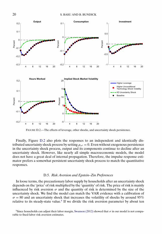
D.5. Risk Aversion and Epstein–Zin Preferences

In loose terms, the precautionary labor supply by households after an uncertainty shockdepends on the ‘price’ of risk multiplied by the ‘quantity’ of risk. The price of risk is mainlyinfluenced by risk aversion σ and the quantity of risk is determined by the size of theuncertainty shock. We find the model can match the VAR evidence with a calibration ofσ = 80 and an uncertainty shock that increases the volatility of shocks by around 95%relative to its steady-state value.8 If we divide the risk aversion parameter by about ten

8Since households can adjust their labor margin, Swanson (2012) showed that σ in our model is not compa-rable to fixed-labor risk aversion estimates.

TECHNICAL APPENDIX 21

FIGURE D.3.—The role of Epstein–Zin preferences.

(σ = 8), then Figure D.3 shows that the resulting impulse responses are roughly one-tenthas large as the baseline calibration. However, if we set σ = 8 but dramatically increasethe volatility of the demand shock process, the model can generate responses that look

22 S. BASU AND B. BUNDICK

like the baseline model even with substantially less risk-averse households.9 Thus, theinclusion of Epstein–Zin preferences allow us to match the VAR evidence with smallermovements in the expected volatility of the exogenous shocks.

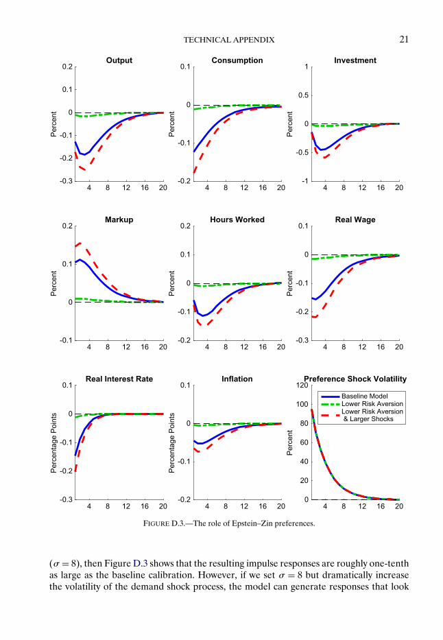
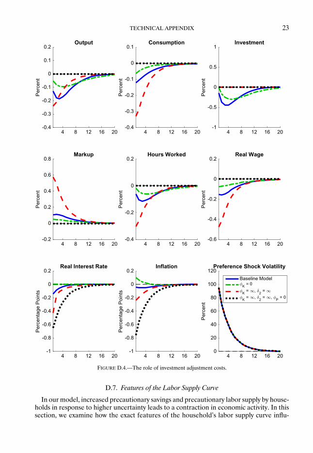
D.6. Investment Adjustment Costs and Variable Capital Utilization

Our baseline model features a very small amount of investment adjustment costs. Toillustrate the role of these adjustment frictions, Figure D.4 shows the impulse responsesto a demand uncertainty shock under two alternative calibrations. In the first alternative,we turn off the adjustment costs completely φK = 0. In the second calibration, we setthe costs of adjusting investment and capital utilization to extremely large values, whichresembles a model with a fixed capital stock.

Investment adjustment costs help the model generate a significant decline in invest-ment after an uncertainty shock. With zero adjustment costs, Figure D.4 shows that theresulting decline in investment is much smaller than our baseline model. Investment ad-justment costs make it more difficult for households to convert their desired savings intophysical assets. Thus, small adjustment frictions cause a larger decline in investment afterthe shock. However, for extremely large adjustment frictions, firms find it too costly to dis-invest. Thus investment stays fixed in response to the uncertainty shock but firms greatlydecrease their demand for household labor. Figure D.4 also shows that investment ad-justment costs are helpful in generating a decline in inflation following an uncertaintyshock.

Without the ability to adjust capital or utilization, the fixed capital stock calibrationresembles a simple New Keynesian model without capital. Figure D.4 plots the impulseresponses for this fixed capital model under both flexible and sticky prices. When pricesare fully flexible and the capital stock is fixed, higher uncertainty causes a decline in realinterest rates and inflation but output and consumption remain unchanged. When pricesare sticky, an increase in uncertainty looks similar to standard time-preference or discountfactor shock. If the central bank can always close the gap between the real rate and thenatural rate of interest, then higher uncertainty has no effect on output in the economy. Inour companion paper, Basu and Bundick (2015), we examined the effects of uncertaintyshocks in a simple New Keynesian model without capital and discussed the optimal policyresponse to higher uncertainty both at and away from the zero lower bound.

Our baseline model also features variable capital utilization. To illustrate the role ofthis feature, Figure D.5 shows the response to a demand uncertainty shock under ourbaseline calibration and a calibration with a significantly higher value of δ2. As discussedby Christiano, Eichenbaum, and Evans (2005), this parameter controls the elasticity ofcapital utilization with respect to the rental rate. Figure D.5 shows that highly elasticcapital utilization helps generate a larger decline in output and investment in our model.Capacity utilization extends the half-life of price stickiness, and hence the period of timeover which our results diverge substantially from those of a flexible-price model. Undernominal rigidities, firms set prices according to the expected present value of marginalcost. Variable capacity utilization creates an elastic supply of capital services and reducesthe responsiveness of marginal cost to output, just as elastic labor supply does.

9For this exercise, we set σa = 0�0105 and σσa = 0�01 such that, as in the baseline model, an uncertaintyshock raises the preference shock volatility by roughly 95%.

TECHNICAL APPENDIX 23

FIGURE D.4.—The role of investment adjustment costs.

D.7. Features of the Labor Supply Curve

In our model, increased precautionary savings and precautionary labor supply by house-holds in response to higher uncertainty leads to a contraction in economic activity. In thissection, we examine how the exact features of the household’s labor supply curve influ-

24 S. BASU AND B. BUNDICK

FIGURE D.5.—The role of variable capital utilization.

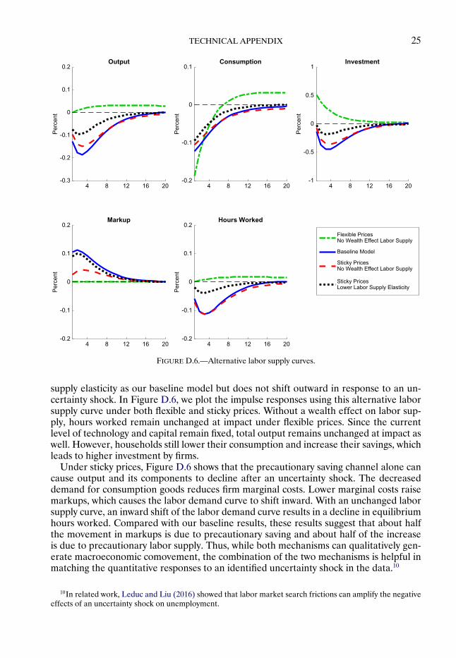
ence the equilibrium outcomes for the macroeconomy. Figure D.6 plots the impulse re-sponses to a demand uncertainty shock under several different labor supply curves. In ourbaseline model, we set the Frisch labor supply elasticity equal to 2. If we instead calibratea labor supply elasticity of one half, Figure D.6 shows that a given uncertainty shock gen-erates smaller movements in output and its components. In terms of the labor supply andlabor demand diagrams from Figure 2 of the main text, a smaller labor supply elasticityimplies a steeper labor supply curve. For given movement in the marginal utility of wealthλt , a steeper labor supply curve implies a much smaller decline in wages and firm marginalcosts.

Households in our model desire to increase saving and labor input in response to anuncertainty shock. To decompose the relative effects of the distinct precautionary laborsupply and precautionary saving channels, we solve a version of our model that does notfeature a wealth effect on labor supply. Taking Appendix Equation (S.5), we divide eachside by its steady-state value and then remove the term involving consumption:

W Rt

W R= 1 −N

1 −Nt

� (S.12)

where W Rt = Wt/Pt denotes the real wage. In the spirit of Greenwood, Hercowitz, and

Huffman (1988) preferences, this alternative labor supply curve features the same labor

TECHNICAL APPENDIX 25

FIGURE D.6.—Alternative labor supply curves.

supply elasticity as our baseline model but does not shift outward in response to an un-certainty shock. In Figure D.6, we plot the impulse responses using this alternative laborsupply curve under both flexible and sticky prices. Without a wealth effect on labor sup-ply, hours worked remain unchanged at impact under flexible prices. Since the currentlevel of technology and capital remain fixed, total output remains unchanged at impact aswell. However, households still lower their consumption and increase their savings, whichleads to higher investment by firms.

Under sticky prices, Figure D.6 shows that the precautionary saving channel alone cancause output and its components to decline after an uncertainty shock. The decreaseddemand for consumption goods reduces firm marginal costs. Lower marginal costs raisemarkups, which causes the labor demand curve to shift inward. With an unchanged laborsupply curve, an inward shift of the labor demand curve results in a decline in equilibriumhours worked. Compared with our baseline results, these results suggest that about halfthe movement in markups is due to precautionary saving and about half of the increaseis due to precautionary labor supply. Thus, while both mechanisms can qualitatively gen-erate macroeconomic comovement, the combination of the two mechanisms is helpful inmatching the quantitative responses to an identified uncertainty shock in the data.10

10In related work, Leduc and Liu (2016) showed that labor market search frictions can amplify the negativeeffects of an uncertainty shock on unemployment.

26 S. BASU AND B. BUNDICK

D.8. Extension to Sticky Nominal Wages

In our baseline model, we generate macroeconomic comovment after an uncertaintyshock by assuming that output prices are sticky, but household wages are fully flexible.However, various types of evidence suggest that nominal wages are sticky, especially athigh frequencies. At the macro level, Christiano, Eichenbaum, and Evans (2005) foundthat nominal wage stickiness is actually more important than nominal price stickiness forexplaining the observed impact of monetary policy shocks. At the micro level, Barattieri,Basu, and Gottschalk (2014) found that the wages of individual workers change less thanonce a year on average.

In this subsection, we show that our results extend readily to the case where nominalwages are sticky. Rather than writing down an extended model with two nominal frictions,we make our point heuristically using the graphical labor supply–labor demand apparatusfrom Section 3 of the main text. If households act competitively in the labor market,

U2(Ct�1 −Nt)= λtWt� (S.13)

whereW is the nominal wage and λt is now the utility value of a marginal dollar. Assumingfirms have market power, we can reorganize Equations (5) and (6) in the main text asfollows:

Wt = Pt

μPtZtF2(Kt�ZtNt)� (S.14)

U2(Ct�1 −Nt)

λtPt= 1μPtZtF2(Kt�ZtNt)� (S.15)

where μPt is the price-markup over marginal cost.Now assume a new model, where households also have market power and set wages

with a markup over their marginal disutility of work. Equation (3) in the main text andthe resulting equilibrium are modified as follows:

Wt = μWtU2(Ct�1 −Nt)

λt� (S.16)

U2(Ct�1 −Nt)

λtPt= 1μWt

1μPtZtF2(Kt�ZtNt)� (S.17)

Compared with the competitive labor market model, we can replace the labor supplycurve in Figure 2 in the main text with U2(Ct�1 −Nt)/λtPt . This quantity has the inter-pretation of the disutility faced by the household of supplying one more unit of labor,expressed in units of real goods (the real marginal cost of supplying labor). On the ver-tical axis, we now plot the equilibrium level of the real marginal disutility of work. Thisalternative ‘supply curve’ is shifted in exactly the same way by uncertainty as the standardlabor supply curve—higher uncertainty raises λ, which shifts the supply curve out. Butnow the ‘demand curve’ in the right-hand side of Equation (S.17) is shifted by both priceand wage markups—only the product of the two matters.

Take the polar opposite of the case we have analyzed so far: Assume perfect compe-tition in product markets but Rotemberg wage setting by monopolistically competitivehouseholds in the labor market. Then, the price markup is always fixed at 1, but the wagemarkup would jump up in response to an increase in uncertainty (since the marginal cost

TECHNICAL APPENDIX 27

of supplying labor falls but the wage is sticky). This alternative assumption would makethe qualitative outcome exactly the same as in our previous results. Thus, while introduc-ing nominal wage stickiness would certainly affect quantitative magnitudes, it would notchange our qualitative results.

APPENDIX E: SOLVING MODEL WITH A ZERO LOWER BOUND CONSTRAINT

To analyze the impact of uncertainty shocks at the zero lower bound, we solve ourmodel using the policy function iteration method of Coleman (1990) and Davig (2004).This global approximation method allows us to model the occasionally-binding zero lowerbound constraint. To make the model computationally feasible using policy function iter-ation, we simplify our baseline model by removing technology shocks and leverage. Wealso assume that households receive firm dividends as a lump-sum payment. Finally, wekeep the number of grid points reasonable by slightly lowering our risk aversion param-eter σ = 15, increasing the amount of investment adjustment costs φK = 10, and slightlyreducing the size of the uncertainty shocks σσa = 0�0015.

The policy function algorithm is implemented using the following steps:1. Discretize the state variables of the model: {Kt ×Yt−1 × at × σat }.2. Conjecture initial guesses for the policy functions of the model Nt = N(Kt�Yt−1�

at�σat ), Ut = U(Kt�Yt−1� at�σ

at ), It = I(Kt�Yt−1� at�σ

at ), Πt = Π(Kt�Yt−1� at�σ

at ), and

EtV1−σt+1 =EV (Kt�Yt−1� at�σ

at ).

3. For each point in the discretized state space, substitute the current policy functionsinto the equilibrium conditions of the model. Use interpolation and numerical integrationover the exogenous state variables at and σat to compute expectations for each Eulerequation. This operation generates a nonlinear system of equations. The solution to thissystem of equations provides an updated value for the policy functions at that point in thestate space.

4. Repeat Step (3) for each point in the state space until the policy functions convergeand cease to be updated.We implement the policy function iteration method in FORTRAN using the nonlinearequation solver DNEQNF from the IMSL numerical library. The model is solved usinga Linux computing cluster and the model solution is parallelized using Open MP.

To compute the impulse response of an uncertainty shock at the zero lower bound, wegenerate two time paths for the economy. In the first time path, we simulate an economyhit by a negative first-moment demand shock such that the zero lower bound binds forabout six quarters. In the second time path, we simulate the same first-moment demandshock, but also simulate an uncertainty shock. After the uncertainty shock, neither econ-omy is hit with any further shock. We present the (percent) difference between the timepaths of variables in the two simulations as the impulse response to the uncertainty shockat the zero lower bound. We choose the size of the uncertainty shock such that, at thestochastic steady state, the simplified model generates roughly the same movements inoutput as our baseline model from Section 4.

REFERENCES

ADJEMIAN, S., H. BASTANI, M. JUILLARD, F. KARAMÉ, F. MIHOUBI, G. PERENDIA, J. PFEIFER, M.RATTO, AND S. VILLEMOT (2011): “Dynare: Reference Manual, Version 4.” [12]

BARATTIERI, A., S. BASU, AND P. GOTTSCHALK (2014): “Some Evidence on the Important of Sticky Wages,”American Economic Journal: Macroeconomics, 6, 70–101. [26]

28 S. BASU AND B. BUNDICK

BASU, S., AND B. BUNDICK (2015): “Endogenous Volatility at the Zero Lower Bound: Implications for Stabi-lization Policy,” NBER Working Paper #21838. [22]

BILS, M., P. J. KLENOW, AND B. A. MALIN (2014): “Resurrecting the Role of the Product Market Wedge inRecessions,” NBER Working Paper #20555. [15]

BLOOM, N. (2009): “The Impact of Uncertainty Shocks,” Econometrica, 77 (3), 623–685. [2,6]CALVO, G. A. (1983): “Staggered Prices in a Utility-Maximizing Framework,” Journal of Monetary Economics,

12 (3), 383–398. [11]CHRISTIANO, L. J., M. EICHENBAUM, AND C. L. EVANS (2005): “Nominal Rigidities and the Dynamic Effects

of a Shock to Monetary Policy,” Journal of Political Economy, 113 (1), 1–45. [22,26]COLEMAN, J. W. (1990): “Solving the Stochastic Growth Model by Policy Function Iteration,” Journal of Busi-

ness & Economic Statistics, 8 (1), 27–29. [27]DAVIG, T. (2004): “Regime-Switching Debt and Taxation,” Journal of Monetary Economics, 51 (4), 837–859.

[27]FERNÁNDEZ-VILLAVERDE, J., P. A. GUERRÓN-QUINTANA, J. RUBIO-RAMÍREZ, AND M. URIBE (2011): “Risk

Matters: The Real Effects of Volatility Shocks,” American Economic Review, 101, 2530–2561. [12]GREENWOOD, J., Z. HERCOWITZ, AND G. W. HUFFMAN (1988): “Investment, Capacity Utilization, and the

Real Business Cycle,” American Economic Review, 78 (3), 402–417. [24]IRELAND, P. N. (2003): “Endogenous Money or Sticky Prices,” Journal of Monetary Economics, 50, 1623–1648.

[7](2011): “A New Keynesian Perspective on the Great Recession,” Journal of Money, Credit, and Bank-

ing, 43 (1), 31–54. [7]JERMANN, U. J. (1998): “Asset Pricing in Production Economies,” Journal of Monetary Economics, 41 (2), 257–

275. [7,10,18]KOOP, G., M. H. PESARAN, AND S. M. POTTER (1996): “Impulse Response Analysis in Nonlinear Multivariate

Models,” Journal of Econometrics, 74, 119–147. [12]LEDUC, S., AND Z. LIU (2016): “Uncertainty Shocks Are Aggregate Demand Shock,” Journal of Monetary

Economics, 82, 20–35. [25]MODIGLIANI, F., AND M. MILLER (1958): “The Cost of Capital, Corporation Finance and the Theory of In-

vestment,” American Economic Review, 48 (3), 261–297. [10,18]ROTEMBERG, J. J. (1982): “Sticky Prices in the United States,” Journal of Political Economy, 90, 1187–1211. [7,

11]SIMS, C. A., AND T. ZHA (1999): “Error Bands for Impulse Responses,” Econometrica, 67 (5), 1113–1155. [1]STOCK, J. H., AND M. W. WATSON (2010): “Research Memorandum.” Available at http://www.princeton.edu/

~mwatson/mgdp_gdi/Monthly_GDP_GDI_Sept20.pdf. [4]SWANSON, E. T. (2012): “Risk Aversion, Risk Premia, and the Labor Margin With Generalized Recursive

Preferences,” American Economic Review, 102, 1663–1691. [20]WU, J. C., AND F. D. XIA (2016): “Measuring the Macroeconomic Impact of Monetary Policy at the Zero

Lower Bound,” Journal of Money, Credit, and Banking, 48 (2–3), 253–291. [1,5]

Dept. of Economics, Boston College, Chestnut Hill, MA 02467, U.S.A. and NationalBureau of Economic Research, Cambridge, MA 02138, U.S.A.; susanto.basu@bc.edu;http://www.bc.edu/schools/cas/economics/ faculty-and-staff/faculty-listing/basu-susanto.html;http://www.nber.org/people/susanto_basu

andFederal Reserve Bank of Kansas City, 1 Memorial Drive, Kansas City, MO 64198, U.S.A.;

brent.bundick@kc.frb.org; https://www.kansascityfed.org/people/brentbundick.

Co-editor Giovanni L. Violante handled this manuscript.

Manuscript received 19 November, 2015; final version accepted 30 November, 2016; available online 10 January,2017.