supervised learning (contd) linear separation
TRANSCRIPT
Supervised Learning (contd)
Linear Separation
Mausam
(based on slides by UW-AI faculty)
1
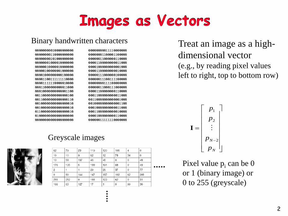
Images as VectorsBinary handwritten characters
Greyscale images
Treat an image as a high-
dimensional vector (e.g., by reading pixel values
left to right, top to bottom row)
N
N
p
p
p
p
2
2
1
I
Pixel value pi can be 0
or 1 (binary image) or
0 to 255 (greyscale)
2
The human brain is extremely good at classifying images
Can we develop classification methods by emulating the brain?
3

Human brain contains a massively
interconnected net of 1010-1011 (10 billion)
neurons (cortical cells)
Biological Neuron
- The simple “arithmetic computing”
element
Brain Computer: What is it?
4
5
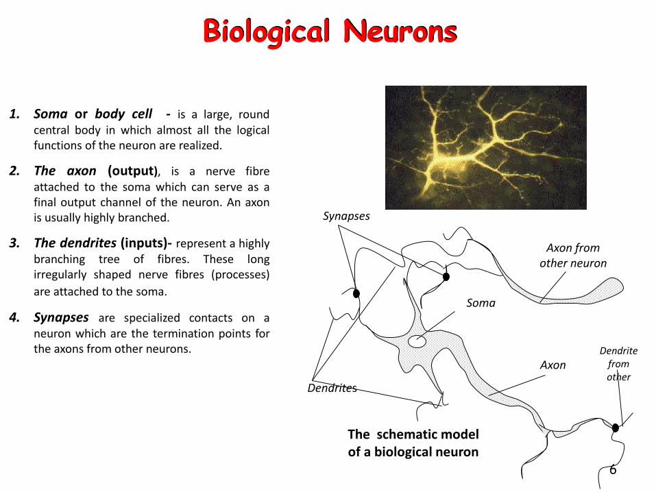
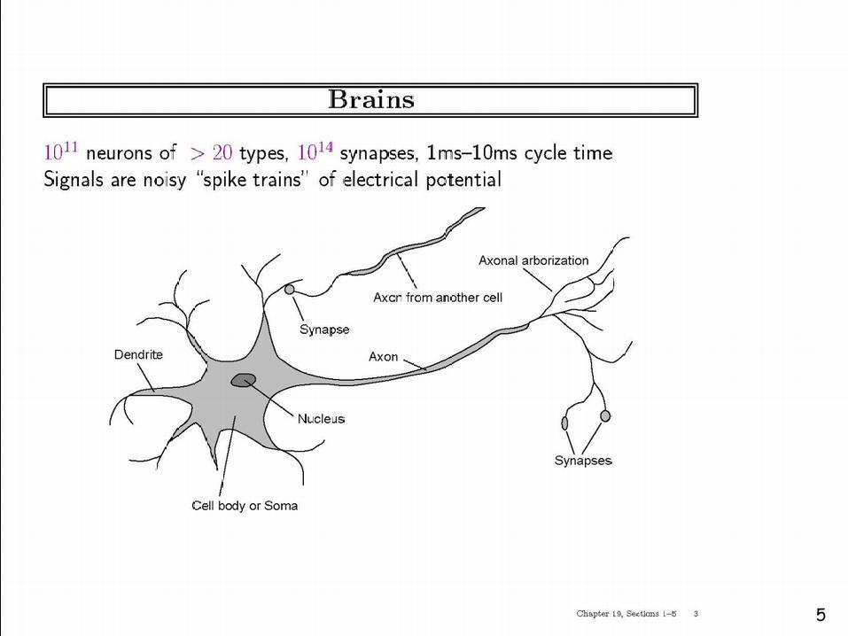
The schematic model of a biological neuron
Synapses
Dendrites
Soma
AxonDendrite
from other
Axon from other neuron
1. Soma or body cell - is a large, roundcentral body in which almost all the logicalfunctions of the neuron are realized.
2. The axon (output), is a nerve fibreattached to the soma which can serve as afinal output channel of the neuron. An axonis usually highly branched.
3. The dendrites (inputs)- represent a highlybranching tree of fibres. These longirregularly shaped nerve fibres (processes)
are attached to the soma.
4. Synapses are specialized contacts on aneuron which are the termination points forthe axons from other neurons.
Biological Neurons
6

Neurons communicate via spikes
Inputs
Output spike
(electrical pulse)
Output spike roughly dependent on whether sum of all inputs reaches a threshold
7
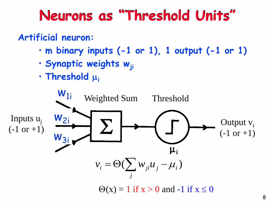
Neurons as “Threshold Units”
Artificial neuron:
• m binary inputs (-1 or 1), 1 output (-1 or 1)
• Synaptic weights wji
• Threshold i
Inputs uj
(-1 or +1)Output vi
(-1 or +1)
Weighted Sum Thresholdw1i
(x) = 1 if x > 0 and -1 if x 0
)( ij
j
jii uwv
w2i
w3i
8
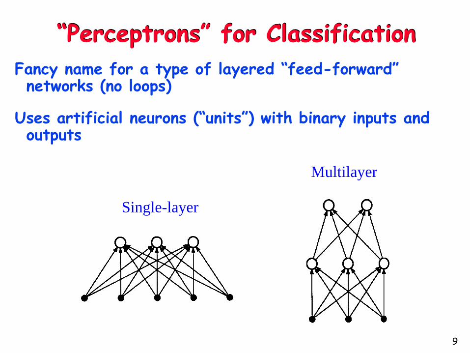
“Perceptrons” for Classification
Fancy name for a type of layered “feed-forward” networks (no loops)
Uses artificial neurons (“units”) with binary inputs and outputs
Multilayer
Single-layer
9
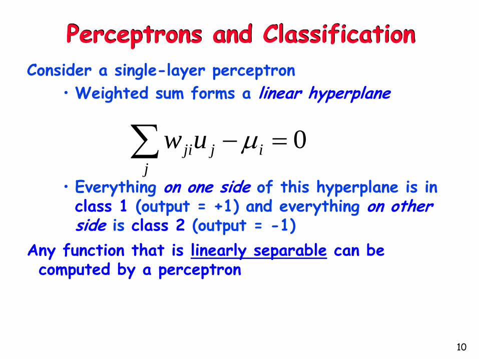
Perceptrons and Classification
Consider a single-layer perceptron
• Weighted sum forms a linear hyperplane
• Everything on one side of this hyperplane is in class 1 (output = +1) and everything on other side is class 2 (output = -1)
Any function that is linearly separable can be computed by a perceptron
0 ij
j
jiuw
10
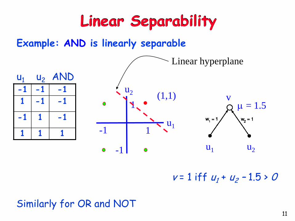
Linear Separability
Example: AND is linearly separable
Linear hyperplane
v
u1 u2
= 1.5(1,1)
1
-1
1
-1u1
u2-1 -1 -1
1 -1 -1
-1 1 -1
1 1 1
u1 u2 AND
v = 1 iff u1 + u2 – 1.5 > 0
Similarly for OR and NOT11

How do we learn the appropriate weights given only examples of
(input,output)?
Idea: Change the weights to decrease the error in output
12
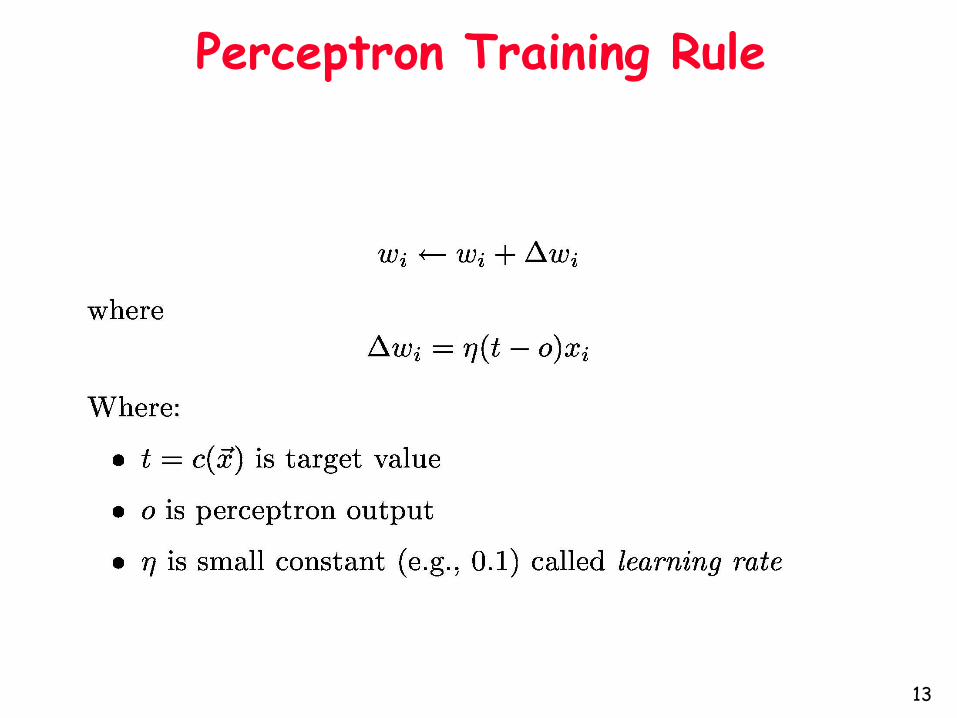
Perceptron Training Rule
13

What about the XOR function?
(1,1)
1
-1
1
-1u1
u2-1 -1 1
1 -1 -1
-1 1 -1
1 1 1
u1 u2 XOR
Can a perceptron separate the +1 outputs from the -1 outputs?
?
14
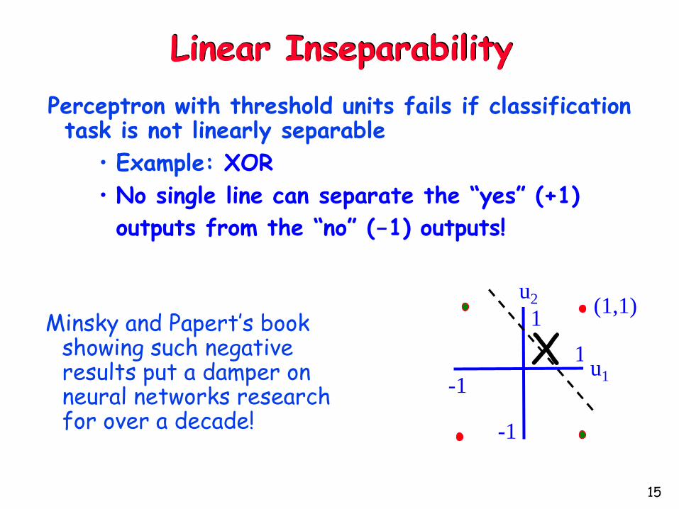
Linear Inseparability
Perceptron with threshold units fails if classification task is not linearly separable
• Example: XOR
• No single line can separate the “yes” (+1)
outputs from the “no” (-1) outputs!
Minsky and Papert’s book showing such negative results put a damper on neural networks research for over a decade!
(1,1)
1
-1
1
-1u1
u2
X
15
How do we deal with linear inseparability?
16
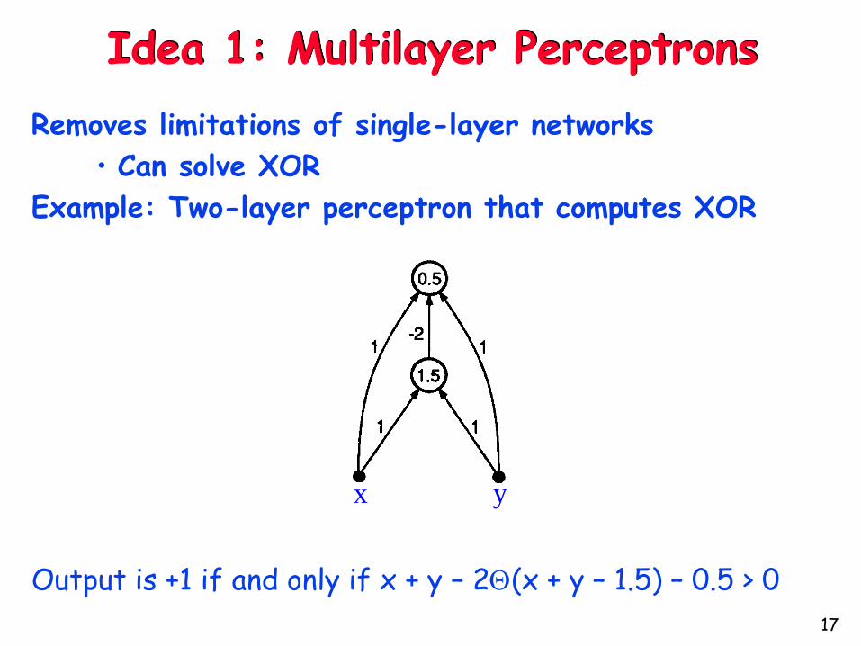
Idea 1: Multilayer Perceptrons
Removes limitations of single-layer networks
• Can solve XOR
Example: Two-layer perceptron that computes XOR
Output is +1 if and only if x + y – 2(x + y – 1.5) – 0.5 > 0
x y
17

x y
out
x
y
1
1
2
1 2
2
1
1
1 1
2
1
11
2
1
?
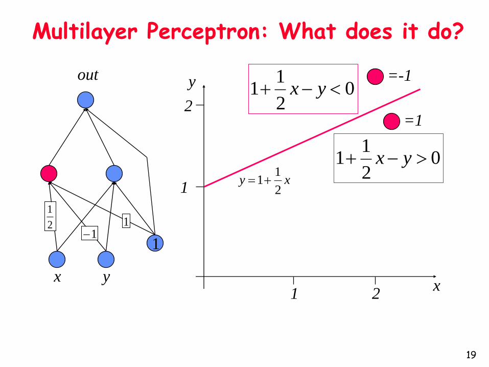
Multilayer Perceptron: What does it do?
18
x y
out
x
y
1
1
2
1 2
02
11 yx
02
11 yx
=-1
=1
2
1
11
xy2
11
Multilayer Perceptron: What does it do?
19
x y
out
x
y
1
1
2
1 2
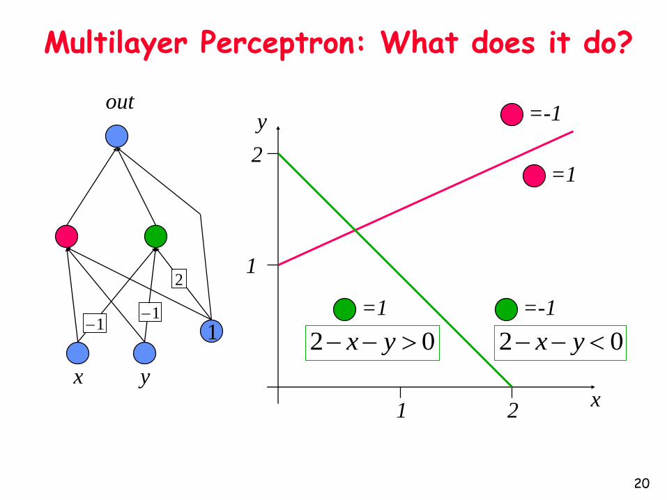
02 yx 02 yx
=-1
=-1=1
=1
1
2
1
Multilayer Perceptron: What does it do?
20

x y
out
x
y
1
1
2
1 2
=-1
=-1=1
=1
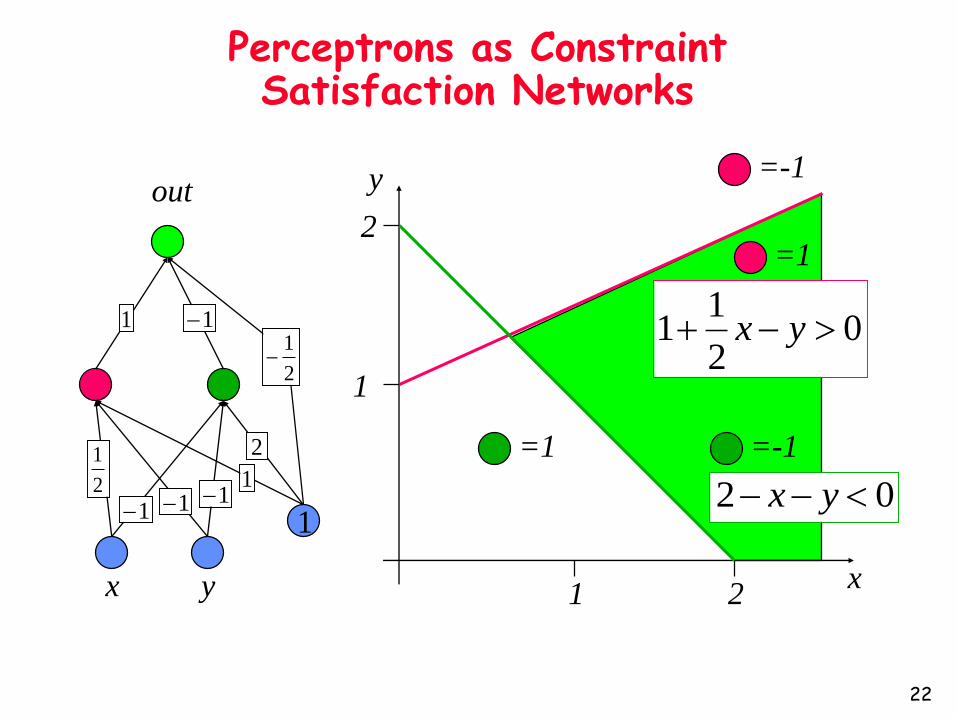
11
2
1 -
2
1 >0
Multilayer Perceptron: What does it do?
21
x y
out
x
y
1
1
2
1 2
02 yx
02
11 yx
=-1
=-1=1
=1
2
1
1
1 1
2
1
11
2
1
Perceptrons as Constraint Satisfaction Networks
22

z z
Linear activation
Threshold activation Hyperbolic tangent activation
Logistic activation
u
u
e
eutanhu
2
2
1
1
1
1 zz
e
1, 0,
sign( )1, 0.
if zz z
if z
z
z
z
z
1
-1
1
0
0
Σ
1
-1
Artificial Neuron:Most Popular Activation Functions
23
Neural Network Issues
• Multi-layer perceptrons can represent any function
• Training multi-layer perceptrons hard
• Backpropagation
• Early successes
• Keeping the car on the road
• Difficult to debug
• Opaque
24
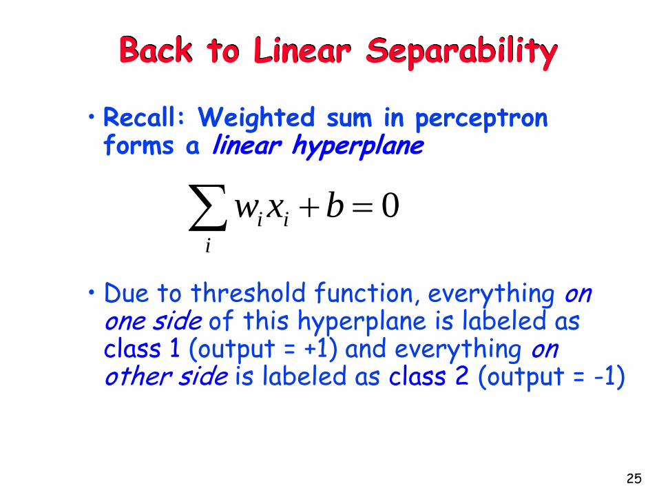
Back to Linear Separability
• Recall: Weighted sum in perceptron forms a linear hyperplane
• Due to threshold function, everything on one side of this hyperplane is labeled as class 1 (output = +1) and everything on other side is labeled as class 2 (output = -1)
0 bxw i
i
i
25
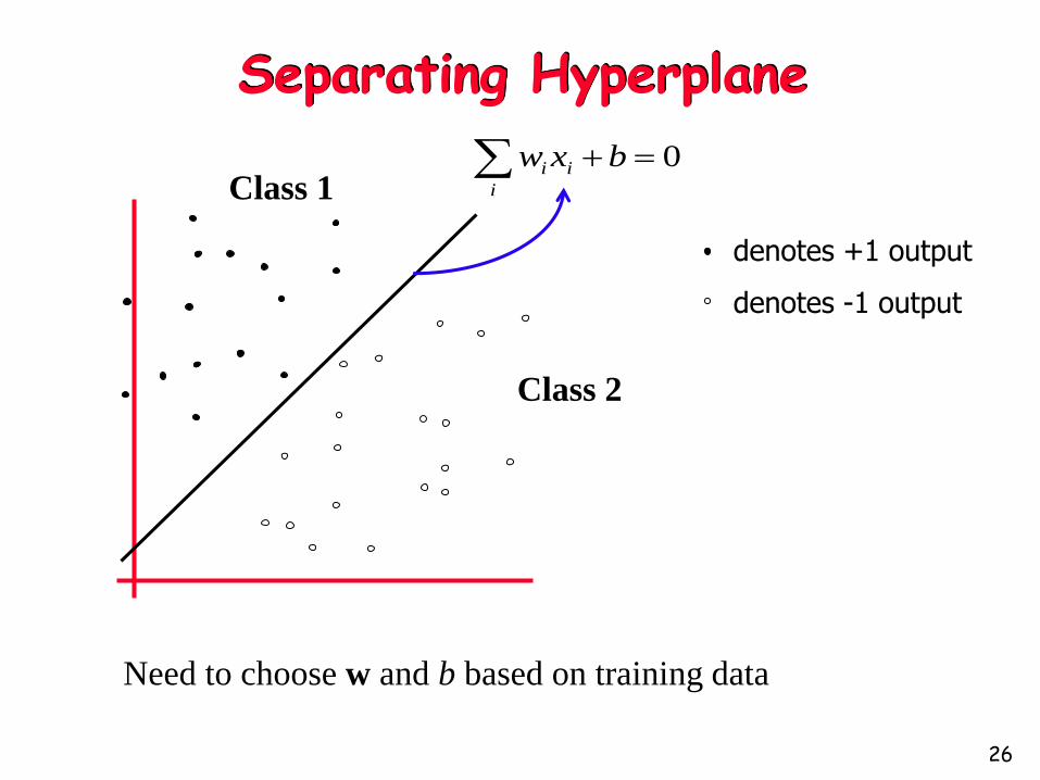
Separating Hyperplane
denotes +1 output
denotes -1 output
Class 2
Need to choose w and b based on training data
0 bxw i
i
i
Class 1
26

Separating Hyperplanes
Different choices of w and b give different hyperplanes
(This and next few slides adapted from Andrew Moore’s)
denotes +1 output
denotes -1 output
Class 1
Class 2
27
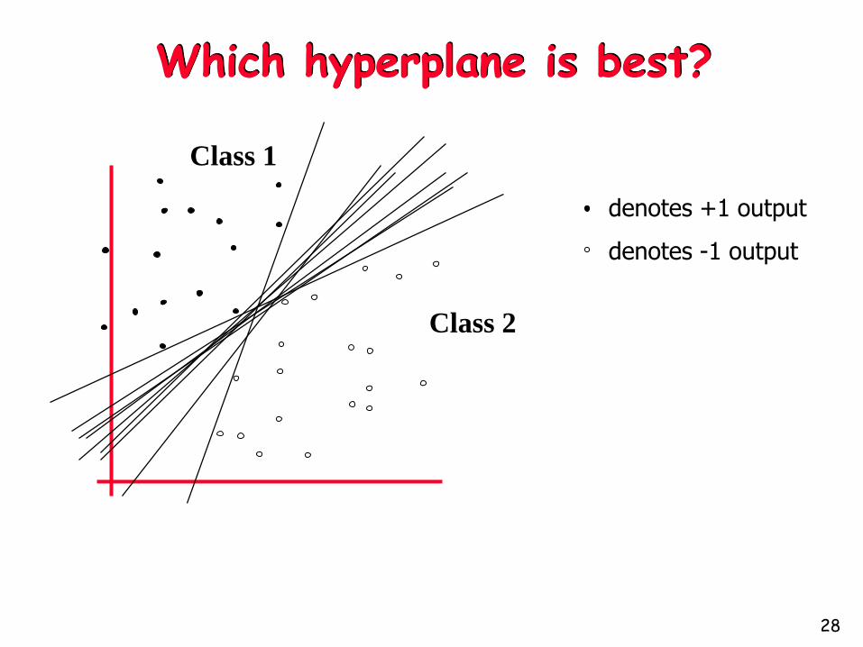
Which hyperplane is best?
denotes +1 output
denotes -1 output
Class 1
Class 2
28

How about the one right in the middle?
Intuitively, this boundary
seems good
Avoids misclassification of
new test points if they are
generated from the same
distribution as training points
29

Margin
Define the marginof a linear classifier as the width that the boundary could be increased by before hitting a datapoint.
30

Maximum Margin and Support Vector Machine
The maximum margin classifier is called a Support Vector Machine (in this case, a Linear SVM or LSVM)
Support Vectors are those datapoints that the margin pushes up against
31

Why Maximum Margin?
• Robust to small perturbations of data points near boundary
• There exists theory showing this is best for generalization to new points
• Empirically works great
32
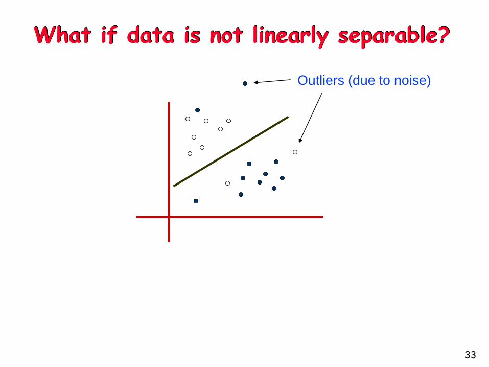
What if data is not linearly separable?
Outliers (due to noise)
33
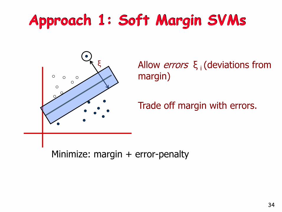
Approach 1: Soft Margin SVMs
Allow errors ξ i (deviations from margin)
Trade off margin with errors.
Minimize: margin + error-penalty
ξ
34

Not linearly separable
What if data is not linearly separable: Other ideas?
36
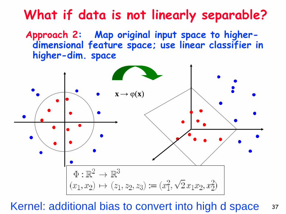
Approach 2: Map original input space to higher-dimensional feature space; use linear classifier in higher-dim. space
x→ φ(x)
What if data is not linearly separable?
Kernel: additional bias to convert into high d space 37
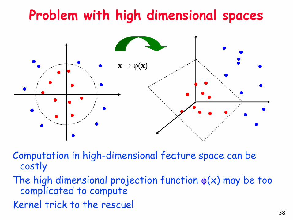
x→ φ(x)
Problem with high dimensional spaces
Computation in high-dimensional feature space can be costly
The high dimensional projection function φ(x) may be too complicated to compute
Kernel trick to the rescue!38
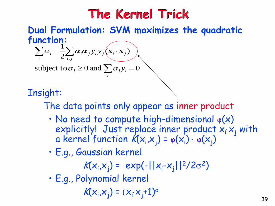
The Kernel TrickDual Formulation: SVM maximizes the quadratic function:
Insight:
The data points only appear as inner product
• No need to compute high-dimensional φ(x) explicitly! Just replace inner product xixj with a kernel function K(xi,xj) = φ(xi) φ(xj)
• E.g., Gaussian kernel
K(xi,xj) = exp(-||xi-xj||2/22)
• E.g., Polynomial kernel
K(xi,xj) = xixj+1)d
i
iii
ji
jijiji
i
i
y
yy
0 and 0 subject to
)(2
1
,
xx
39
K-Nearest Neighbors
A simple non-parametric classification algorithm
Idea:
• Look around you to see how your neighbors classify data
• Classify a new data-point according to a majority vote of your k nearest neighbors
41
Distance Metric
How do we measure what it means to be a neighbor (what is “close”)?
Appropriate distance metric depends on the problem
Examples:
x discrete (e.g., strings): Hamming distanced(x1,x2) = # features on which x1 and x2 differ
x continuous (e.g., vectors over reals): Euclidean distance
d(x1,x2) = || x1-x2 || = square root of sum of squared differences between corresponding elements of data vectors
42
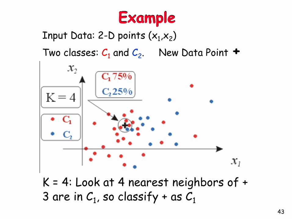
ExampleInput Data: 2-D points (x1,x2)
Two classes: C1 and C2. New Data Point +
K = 4: Look at 4 nearest neighbors of +3 are in C1, so classify + as C1
43

Decision Boundary using K-NN
Some points near the boundary may be misclassified
(but maybe noise)
44

What if we want to learn continuous-valued functions?
Input
Output
45
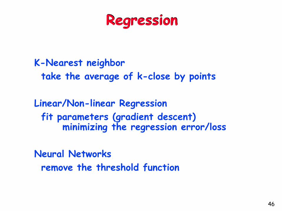
Regression
K-Nearest neighbor
take the average of k-close by points
Linear/Non-linear Regression
fit parameters (gradient descent) minimizing the regression error/loss
Neural Networks
remove the threshold function
46
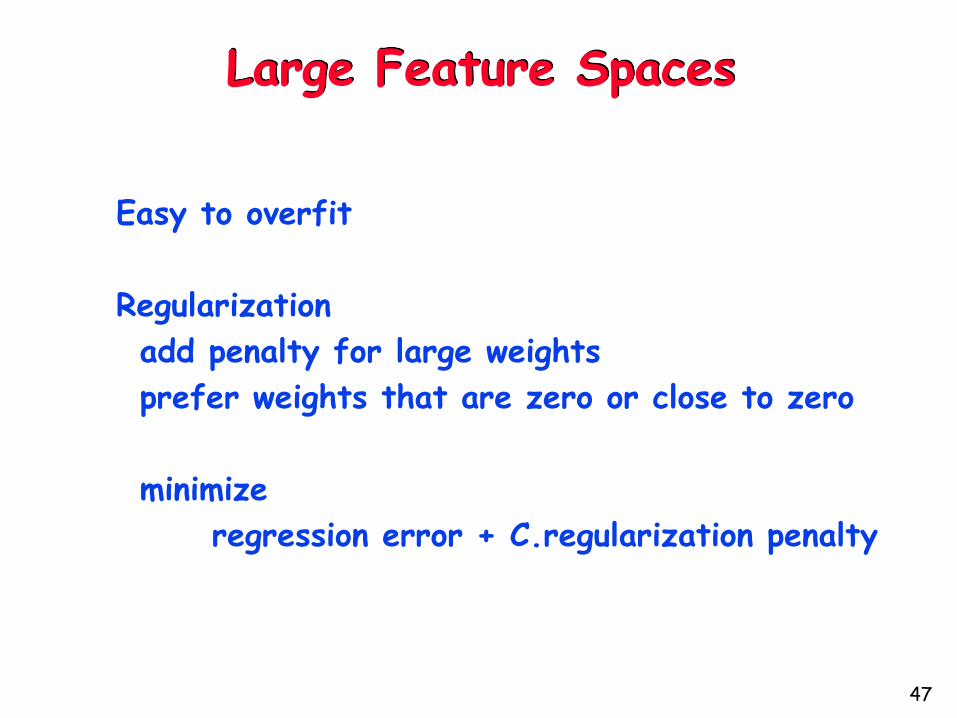
Large Feature Spaces
Easy to overfit
Regularization
add penalty for large weights
prefer weights that are zero or close to zero
minimize
regression error + C.regularization penalty
47
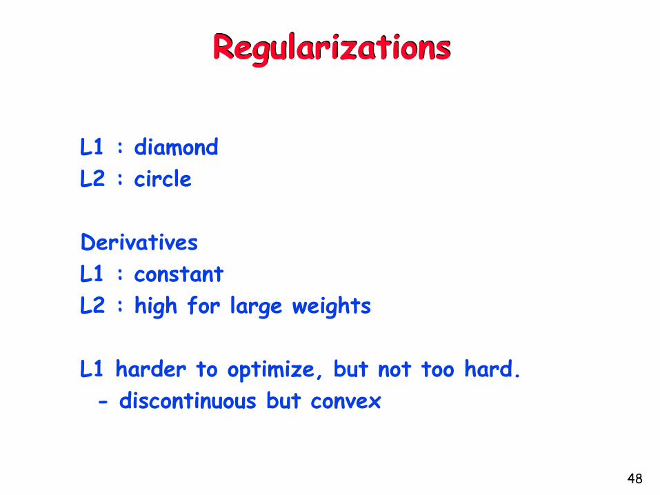
Regularizations
L1 : diamond
L2 : circle
Derivatives
L1 : constant
L2 : high for large weights
L1 harder to optimize, but not too hard.
- discontinuous but convex
48
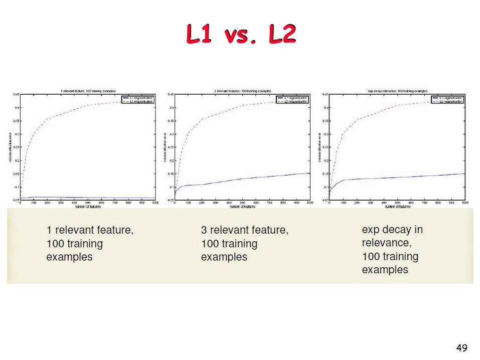
L1 vs. L2
49
Supervised Learning (contd)
Decision Trees
Mausam
(based on slides by UW-AI faculty)

51
Decision Trees
To play or
not to play?
http://www.sfgate.com/blogs/images/sfgate/sgreen/2007/09/05/2240773250x321.jpg

52
Example data for learning the concept “Good day for tennis”
Day Outlook Humid Wind PlayTennis?d1 s h w nd2 s h s nd3 o h w yd4 r h w yd5 r n w yd6 r n s yd7 o n s yd8 s h w nd9 s n w yd10 r n w yd11 s n s yd12 o h s yd13 o n w yd14 r h s n
• Outlook = sunny, overcast, rain
• Humidity = high, normal
• Wind = weak, strong
53
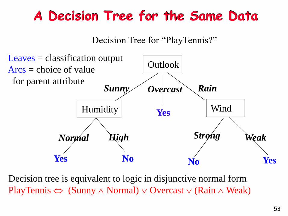
A Decision Tree for the Same Data
Outlook
Humidity Wind
YesYes
Yes
No No
Sunny Overcast Rain
High StrongNormal Weak
Decision Tree for “PlayTennis?”
Leaves = classification output
Arcs = choice of value
for parent attribute
Decision tree is equivalent to logic in disjunctive normal form
PlayTennis (Sunny Normal) Overcast (Rain Weak)
55
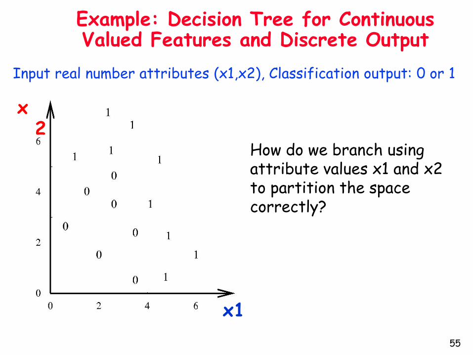
Example: Decision Tree for Continuous Valued Features and Discrete Output
x1
x2
How do we branch using attribute values x1 and x2 to partition the space correctly?
Input real number attributes (x1,x2), Classification output: 0 or 1

56
Example: Classification of Continuous Valued Inputs
3
4
Decision Tree
x1
x2
57
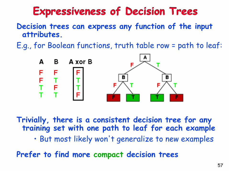
Expressiveness of Decision Trees
Decision trees can express any function of the input attributes.
E.g., for Boolean functions, truth table row = path to leaf:
Trivially, there is a consistent decision tree for any training set with one path to leaf for each example
• But most likely won't generalize to new examples
Prefer to find more compact decision trees

58
Learning Decision Trees
Example: When should I wait for a table at a restaurant?
Attributes (features) relevant to Wait? decision:
1. Alternate: is there an alternative restaurant nearby?
2. Bar: is there a comfortable bar area to wait in?
3. Fri/Sat: is today Friday or Saturday?
4. Hungry: are we hungry?
5. Patrons: number of people in the restaurant (None, Some, Full)
6. Price: price range ($, $$, $$$)
7. Raining: is it raining outside?
8. Reservation: have we made a reservation?
9. Type: kind of restaurant (French, Italian, Thai, Burger)
10. WaitEstimate: estimated waiting time (0-10, 10-30, 30-60, >60)

59
Example Decision tree
A decision tree for Wait? based on personal “rules of thumb”:
60
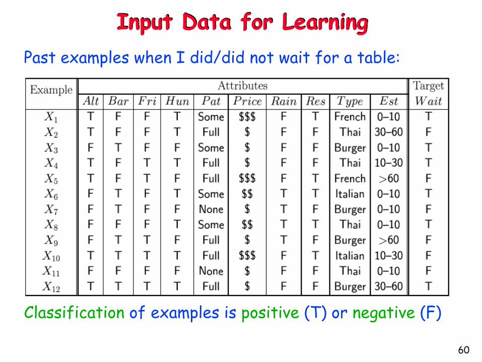
Input Data for Learning
Past examples when I did/did not wait for a table:
Classification of examples is positive (T) or negative (F)

61
Decision Tree Learning
Aim: find a small tree consistent with training examples
Idea: (recursively) choose "most significant" attribute as root of (sub)tree
62
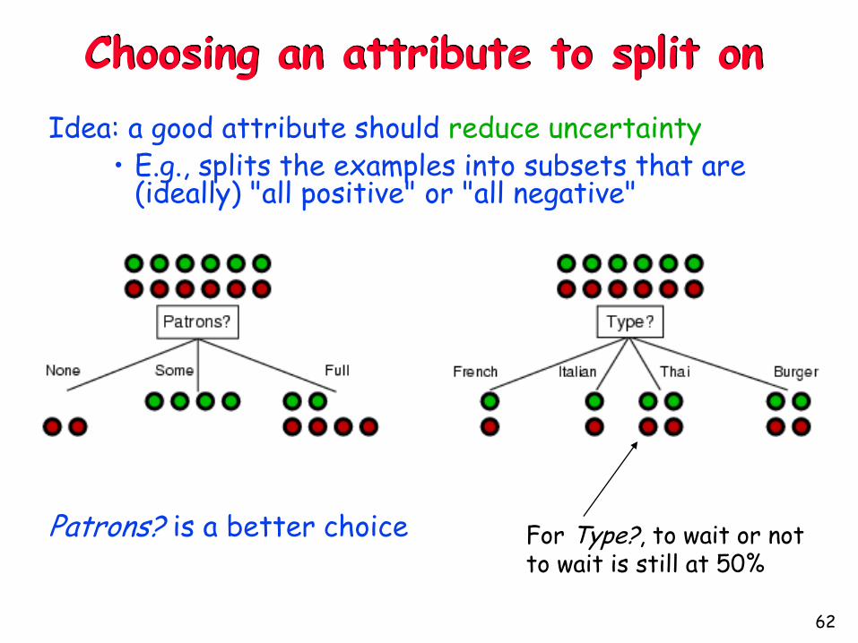
Choosing an attribute to split on
Idea: a good attribute should reduce uncertainty• E.g., splits the examples into subsets that are
(ideally) "all positive" or "all negative"
Patrons? is a better choice For Type?, to wait or not to wait is still at 50%
How do we quantify uncertainty?
http://a.espncdn.com/media/ten/2006/0306/photo/g_mcenroe_195.jpg

64
Using information theory to quantify uncertainty
Entropy measures the amount of uncertainty in a probability distribution
Entropy (or Information Content) of an answer to a question with possible answers v1, … , vn:
I(P(v1), … , P(vn)) = Σi=1 -P(vi) log2 P(vi)
65
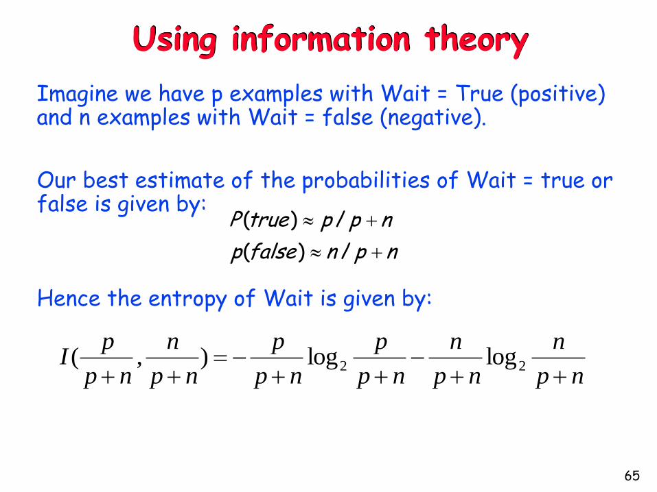
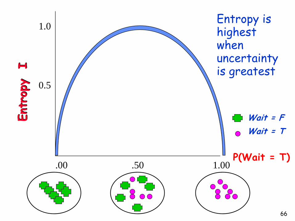
Using information theory
Imagine we have p examples with Wait = True (positive) and n examples with Wait = false (negative).
Our best estimate of the probabilities of Wait = true or false is given by:
Hence the entropy of Wait is given by:
( ) /
( ) /
P true p p n
p false n p n
np
n
np
n
np
p
np
p
np
n
np
pI
22 loglog),(
66
P(Wait = T)
Ent
ropy
I
.00 .50 1.00
1.0
0.5
Entropy is highest when uncertainty is greatest
Wait = T
Wait = F

67
Idea: a good attribute should reduce uncertainty and result in “gain in information”
How much information do we gain if we disclose the value of some attribute?
Answer:
uncertainty before – uncertainty after
Choosing an attribute to split on

68
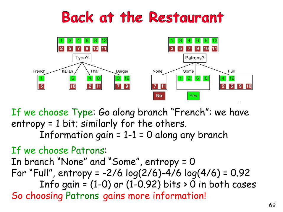
Back at the Restaurant
Before choosing an attribute:
Entropy = - 6/12 log(6/12) – 6/12 log(6/12)
= - log(1/2) = log(2) = 1 bit
There is “1 bit of information to be discovered”
69
Back at the Restaurant
If we choose Type: Go along branch “French”: we have entropy = 1 bit; similarly for the others.
Information gain = 1-1 = 0 along any branch
If we choose Patrons: In branch “None” and “Some”, entropy = 0 For “Full”, entropy = -2/6 log(2/6)-4/6 log(4/6) = 0.92
Info gain = (1-0) or (1-0.92) bits > 0 in both casesSo choosing Patrons gains more information!
70
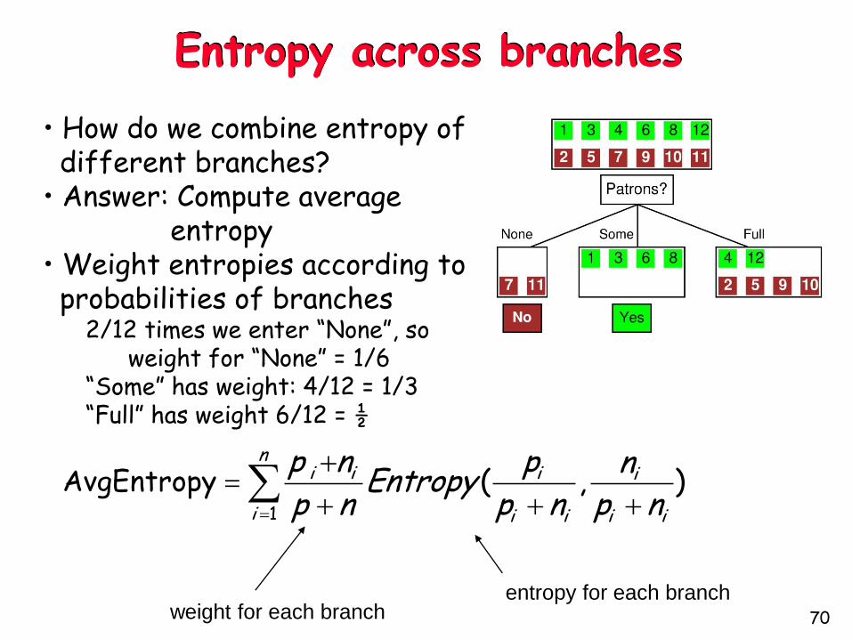
Entropy across branches
• How do we combine entropy of different branches?
• Answer: Compute average entropy
• Weight entropies according to probabilities of branches
2/12 times we enter “None”, so weight for “None” = 1/6
“Some” has weight: 4/12 = 1/3“Full” has weight 6/12 = ½
1
( ) ( , )n
i i i i
i i i i i
p n p nEntropy A Entropy
p n p n p n
weight for each branch entropy for each branch
AvgEntropy
71
Information gain
Information Gain (IG) or reduction in entropy from using attribute A:
Choose the attribute with the largest IG
IG(A) = Entropy before – AvgEntropy after choosing A

72
Information gain in our example
Patrons has the highest IG of all attributes
DTL algorithm chooses Patrons as the root
bits 0)]4
2,
4
2(
12
4)
4
2,
4
2(
12
4)
2
1,
2
1(
12
2)
2
1,
2
1(
12
2[1)(
bits 541.)]6
4,
6
2(
12
6)0,1(
12
4)1,0(
12
2[1)(
IIIITypeIG
IIIPatronsIG
73
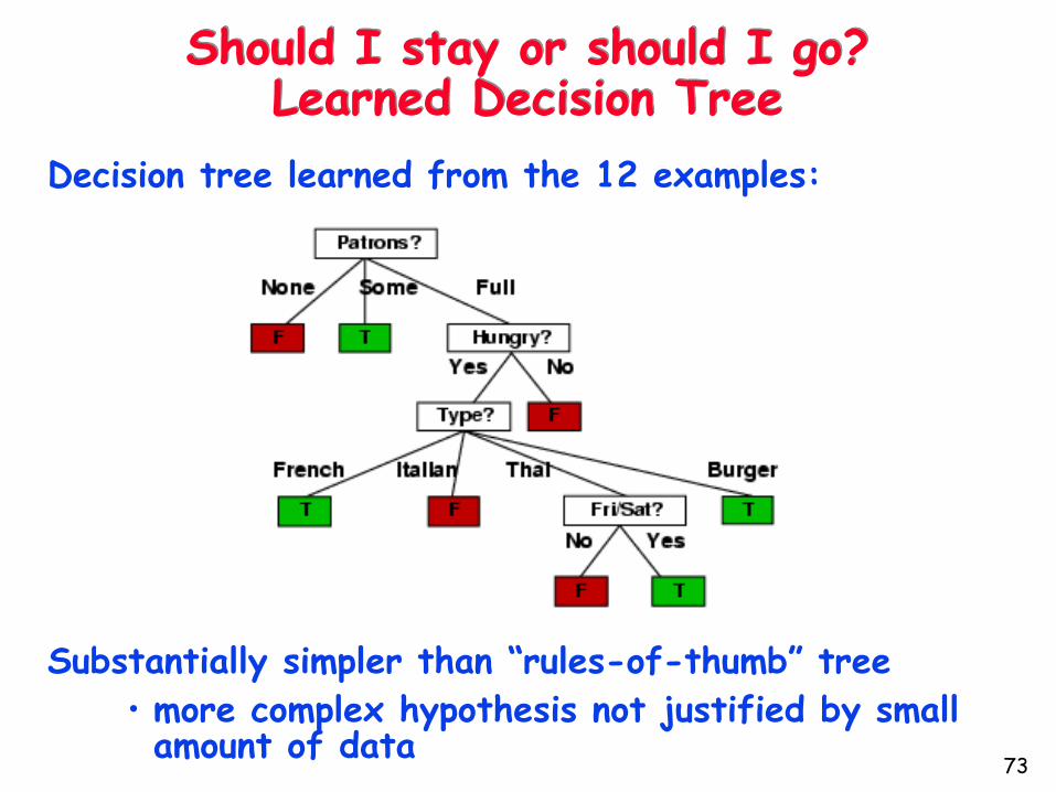
Decision tree learned from the 12 examples:
Substantially simpler than “rules-of-thumb” tree
• more complex hypothesis not justified by small amount of data
Should I stay or should I go?Learned Decision Tree

74
Performance Evaluation
How do we know that the learned tree h ≈ f ?
Answer: Try h on a new test set of examples
Learning curve = % correct on test set as a function of training set size
75
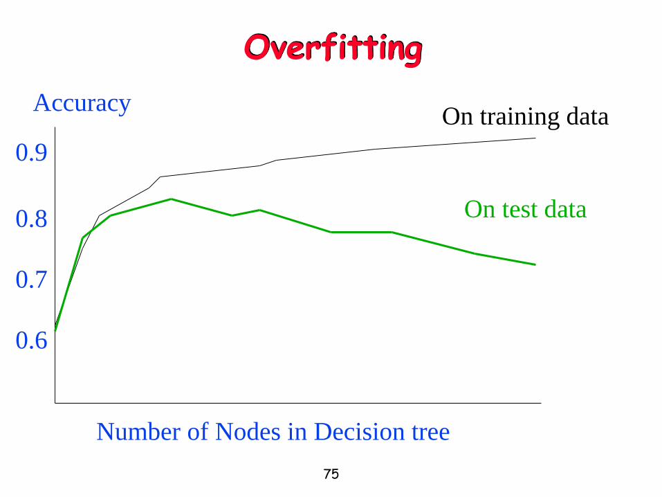
Overfitting
Number of Nodes in Decision tree
Accuracy
0.9
0.8
0.7
0.6
On training data
On test data

76
Rule #2 of Machine Learning
The best hypothesis almost never achieves 100% accuracy on the training data.
(Rule #1 was: you can’t learn anything without inductive bias)
77
Avoiding overfitting
78
• Stop growing when data split not statistically significant
• Grow full tree and then prune
•How to select best tree?
•Measure performance over the training data
•Measure performance over separate validation set
•Add complexity penalty to performance measure
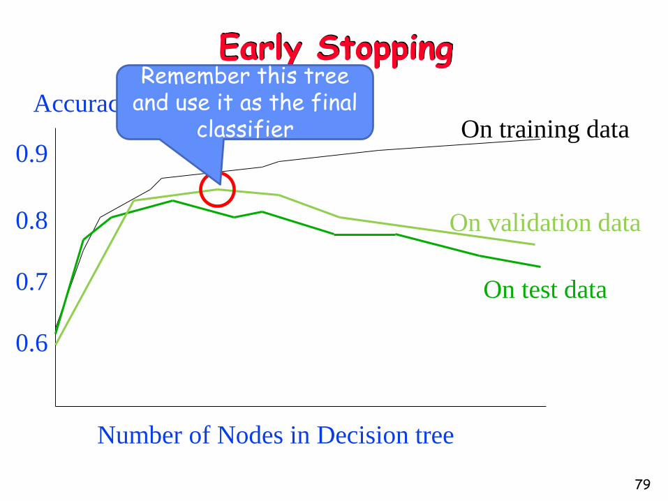
Early Stopping
Number of Nodes in Decision tree
Accuracy
0.9
0.8
0.7
0.6
On training data
On validation data
On test data
Remember this tree and use it as the final
classifier
79
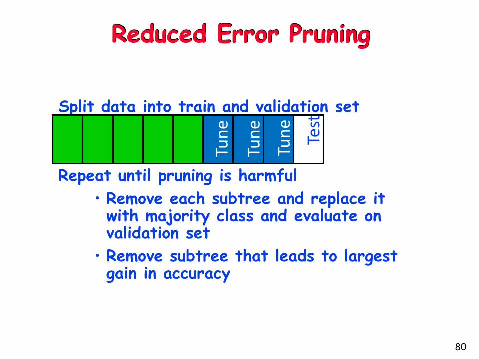
Reduced Error Pruning
Split data into train and validation set
Repeat until pruning is harmful
• Remove each subtree and replace it with majority class and evaluate on validation set
• Remove subtree that leads to largest gain in accuracy
Test
Tun
e
Tun
e
Tun
e
80
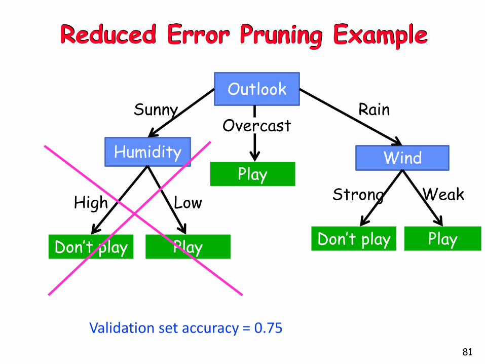
Reduced Error Pruning Example
Outlook
Humidity Wind
Sunny RainOvercast
High Low WeakStrong
Play
Play
Don’t play PlayDon’t play
Validation set accuracy = 0.75
81

Reduced Error Pruning Example
Outlook
Wind
Sunny RainOvercast
WeakStrongPlay
Don’t play
PlayDon’t play
Validation set accuracy = 0.80
82
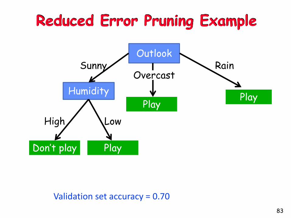
Reduced Error Pruning Example
Outlook
Humidity
Sunny RainOvercast
High Low
Play
Play
Don’t play
Play
Validation set accuracy = 0.70
83
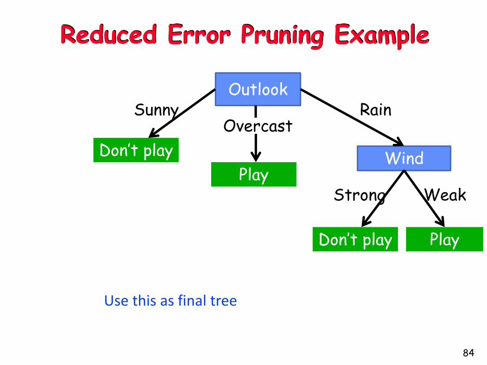
Reduced Error Pruning Example
Outlook
Wind
Sunny RainOvercast
WeakStrongPlay
Don’t play
PlayDon’t play
Use this as final tree
84
Post Rule Pruning
• Split data into train and validation set
• Prune each rule independently
– Remove each pre-condition and evaluate accuracy
– Pick pre-condition that leads to largest improvement in accuracy
• Note: ways to do this using training data and statistical tests
85
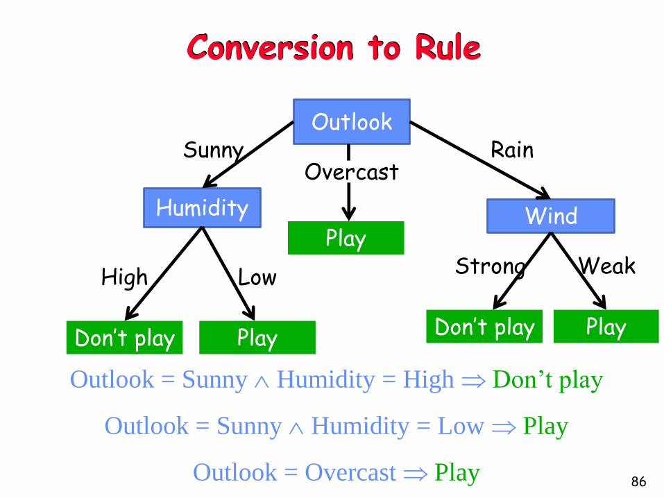
Conversion to Rule
Outlook
Humidity Wind
Sunny RainOvercast
High Low WeakStrong
Play
Play
Don’t play PlayDon’t play
Outlook = Sunny Humidity = High Don’t play
Outlook = Sunny Humidity = Low Play
Outlook = Overcast Play
…
86
Scaling Up
87
• ID3 and C4.5 assume data fits in main memory
(ok for 100,000s examples)
• SPRINT, SLIQ: multiple sequential scans of data
(ok for millions of examples)
• VFDT: at most one sequential scan
(ok for billions of examples)
Decision Trees – Strengths
Very Popular Technique
Fast
Useful when
• Target Function is discrete
• Concepts are likely to be disjunctions
• Attributes may be noisy
88

Decision Trees – Weaknesses
Less useful for continuous outputs
Can have difficulty with continuous input features as well…
• E.g., what if your target concept is a circle in the x1, x2 plane?– Hard to represent with decision trees…
– Very simple with instance-based methods we’ll discuss later…
89