sums of squares over function fields kathy merrill and

SUMS OF SQUARES OVER FUNCTION FIELDS

Kathy Merrill and Lynne H. Walling

Given a polynomial α with coefficients in a finite field F, how many ways canwe represent α as a sum of k squares? The answer to this question is all too often“infinity.” Thus instead we ask: What is the value of the “restricted representationnumber”

r(α,m) = #

(β1, . . . , βk) :∑j

β2j = α and deg βj < m

?

Eisenstein [ref?] approached the analogous problem over Z using the arith-metic theory of quadratic forms; this approach was developed further by Smithand Minkowski [ref?], who were able to present formulas to solve the problem fork ≤ 8. Alternatively, Jacobi used the theory of elliptic functions and even powersof the classical theta series, θ(z), solving the problem for k = 2, 4, 6, 8. Hardy calledJacobi’s approach “simpler” than that of Smith and Minkowski, and remarked that“it has another very important merit, that it can be used – within the limits ofhuman capacity for calculation – for any even value of s” (here s = k) [ref: paperstarts on p. 340]. Then in [ref – same as above], Hardy used the theory of ellipticfunctions to treat the case where k =5 or 7. Hardy wrote that the solution tothe problem for k > 8 involves “other and more recondite arithmetical functions”[ref, p. 340?]; still, in [ref #4 cited on p. 344], Hardy and Ramanujan introducedtechniques that led to asymptotic formulas for these representation numbers withk arbitrary (k > 4).

We note here that in light of our present knowledge of holomorphic automorphicforms, it is not surprising that Hardy and Ramanujan obtain only asymptotic for-mulas for k > 8. Their approach involves the study of θ(z)k, which is a holomorphicautomorphic form of weight k

2 for the congruence subgroup Γ0(4). When k ≤ 8and k is even, we know there are no cusp forms for Γ0(4) and thus θ(z)k mustbe an Eisenstein series (whose Fourier coefficients are well understood and easilycomputed). However, when k > 8, θ(z)k is a linear combination of an Eisensteinseries and a cusp form – Hardy’s “recondite” function. The order of magnitude ofthe Fourier coefficients of a cusp form is small compared to that of an Eisensteinseries; thus the Fourier coefficients of θ(z)k are asymptotic to those of the associ-ated Eisenstein series. (To find the dimension of a space of integral weight cuspforms with level and character, one can use the formula found in [Ross] which isderived from Hijikata’s trace formula.)

second author partially supported by NSF grant DMS 9103303

Typeset by AMS-TEX

1

2 KATHY MERRILL AND LYNNE H. WALLING

In this paper we too will use powers of a theta function to study the restrictedrepresentation numbers r(α,m) where α lies in the polynomial ring F[T ] (T anindeterminate); the theta function θ(z) we use was recently presented in [H-R] (seeThm?). After some preliminary remarks, we show that θ(z) transforms like an au-tomorphic form of weight 1/2 under the “full modular group” Γ (see Theorem 2.4).Then using rather elementary techniques, we derive a formula for r(α,m). Thisformula involves Kloosterman sums when degα ≥ 4, but we are able to compute:(1) the average value of r(α,m); (2) the order of magnitude of r(α,m) as m→∞or degα → ∞; and (3) an asymptotic formula for r(α,m) as k, the number ofsquares, approaches ∞ (see Theorems 3.11, 3.14, 3.15 resp.).

For a full account of the history of this problem over Z, the reader is refered to[Grosswald]. To read about automorphic forms over a function field, the reader isrefered to [Weil] and [H-R].

The authors thank Jeff Hoffstein and Jeff Stopple for many helpful conversations.§1. Preliminaries. One of the most intriguing and most studied structures

in number theory is Z, the ring of rational integers. The theory of automorphicforms has provided us with some powerful tools to aid us in our study of Z; see, forexample, [Terras]. We review here the basic classical set-up.

To each of the valuations on Q, the field of fractions of Z, we can associate an“upper half-plane” H = G/K. Here G = PSL2(completion of Q) and K is themaximal compact subgroup of G. An automorphic form on H is a function whichtransforms with a factor of “automorphy” under the action of Γ = SL2(Z) on H,

and is invariant under the subgroup Γ∞ ={(

1 a0 1

): a ∈ Z

}(see [Shimura’s

book] or [Koblitz]).We want to parallel this arrangement to study the polynomial ring, A = F[T ];

here F is a finite field and T is an indeterminate. For the sake of clarity, we treatonly the case where F has p elements, p an odd prime. We denote the field offractions of A by K = F(T ). One of the valuations | · |∞ on K, the “infinite”valuation, is induced by the degree map: for α, β ∈ A, define

|α/β|∞ = pdegα−deg β .

We adopt the convention that deg 0 = −∞, and hence |0|∞ = 0. Note that unlikethe infinite valuation on Q – which is absolute value – this infinite valuation isnonarchimedean; this in fact eases many computations. We let K∞ denote thecompletion of K with respect to | · |∞; one easily sees that K∞ = F(( 1

T )), formalLaurent series in 1

T . The “unit ball” or “ring of integers” in K∞ is

O∞ = {x ∈ K∞ : |x|∞ ≤ 1 } = F[[ 1T ]]

(so O∞ consists of formal Taylor series in 1T ). We note here that O∞ is a discrete

valuation ring with a unique maximal ideal P∞ = {x ∈ K∞ : |x|∞ < 1 } .Let µ be (additive) Haar measure on K∞, normalized so that µ(O∞) = 1. By

the translation invariance of µ, we have that for any a ∈ K∞,

µ ({x : xj = aj for j > n }) = pn.

(Here x =∑j≥−∞ xjT

j .)

SUMS OF SQUARES OVER FUNCTION FIELDS 3

Set G = PSL2(K∞); then the maximal compact subgroup of G (with respect tothe standard? topology induced on G by | · |∞) is PSL2(O∞). Thus we set

H = PSL2(K∞)/PSL2(O∞).

In §2 we will define an automorphic form on H.

Remark. Some authors, like Weil and Ephrat, use PGL instead of PSL in thedefinition of H. While this choice is irrelevent in the construction of the complexupper half-plane, it is not irrelevent in the function field setting.

Proposition 1.1. The set{(y x0 1

): y = T 2m, m ∈ Z, x ∈ T 2m+1

A

}is a complete set of coset representatives for H = PSL2(K∞)/PSL2(O∞).

Proof. Take z =(a bc d

)∈ SL2(K∞). Then

z ≡

(a b

c d

)(1 0− cd 1

)if deg c ≤ deg d,(

a b

c d

)( dc 1−1 0

)if deg d < deg c

where z ≡ z′ means z and z′ represent the same coset of H. Thus z is equivalentto a matrix of the form (

w x′

0 w−1

)with w, x′ ∈ K∞, w 6= 0. Now, w = Tmu for some m ∈ Z and u ∈ O×∞. So

z ≡(w x′

0 w−1

)(u−1 0

0 u

)≡(Tm x′′

0 T−m

)for some x′′ ∈ K∞. Writing x′′ as T−m(x + T 2mv) where x ∈ T 2m+1

A, v ∈ O∞,we see that

z ≡(Tm x′′

0 t−m

)(1 −v0 1

)≡(Tm T−mx0 T−m

)≡(T 2m x

0 1

).

Now suppose z ≡(T 2m x

0 1

)≡(T 2m′ x′

0 1

)where m,m′ ∈ Z, x ∈ T 2m+1

A,

x′ ∈ T 2m′+1A. Then(

Tm T−mx0 T−m

)−1(Tm

′T−m

′x′

0 T−m′

)=(Tm

′−m T 1m′−m(x′ − x)0 Tm−m

′

)∈ SL2(O∞).

Thus Tm′−m, Tm−m

′ ∈ O∞, which implies m = m′. So T−m′−m(x′ − x) =

T−2m(x′ − x) ∈ O∞. We know x, x′ ∈ T 2m+1A, so

T−2m(x′ − x) ∈ O∞ ∩ TA = {0} .


Hence x = x′. �

The group Γ = SL2(A) acts on H by left multiplication. We expect certainfunctions, which we will call automorphic, should transform with some sort offactor of automorphy; these functions should actually be invariant under the actionof

Γ∞ ={(

1 α0 1

): α ∈ A

}.

For such a function f , we fix y = T−2m and let fy be the resulting function

on T 1−2mA given by fy(x) = f

((y x0 1

)). Because of the invariance of f under

Γ∞, we can consider fy as a function on the finite abelian (additive) subgroupT 1−2m

A/A of K∞/A. This makes Fourier series in x a useful tool for analyzingautomorphic forms. Before defining the specific automorphic form we will study,we give a description of Fourier series in this setting.

For x ∈ K∞, write x =∑nj=−∞ xjT

j , and let e{x} = exp{2πix1/p}. We use thisdefinition on K∞/A as well, by making the natural identification between K∞/Aand {x ∈ K∞ : xj = 0 for j ≥ 0}.

Lemma 1.2. The character groups of K∞, K∞/A, and T 1−2mA/A are isomorphic

to K∞, T 2A, and T 2

A/T 2m+1A respectively.

Proof. For β ∈ K∞, let ψβ be defined by ψβ(x) = e{βx}. Each ψβ is clearly acontinuous homomorphism on K∞; by restricting to subgroups of monomials, wesee that all characters of K∞ are of this form. The characters of K∞/A consistof those ψβ which are trivial on A, that is {ψβ : β ∈ T 2

A}. The characters ofT 1−2m

A/A are then obtained by equating characters of K∞/A which agree onT 1−2m

A/A.

Elementary harmonic analysis then leads to the following:

Theorem 1.3. Any function f on H which is invariant under the action of Γ∞

can be expanded in a Fourier series f((

y x0 1

))=∑β∈T 2A cβ(y)χ(βy)e{βx},

where cβ(T−2m) = p1−2m∑x∈T 1−2m

A/A f

((y x0 1

))e{−βx) and χ = χO∞ is the

characteristic function of O∞.

Proof. We fix y = T−2m, and use the Lemma to write

f

((T−2m x

0 1

))= fy(x) =

∑β∈T 2A/T 2m+1A

cβ(T−2m)e{βx}

where cβ(T−2m) = p1−2m∑x∈T 1−2m

A/A fy(x)e{−βx), and where we make the nat-ural identification between β ∈ T 2

A/T 2m+1A and {β ∈ T 2

A : βj = 0 for j > 2m}.The theorem then follows by noting that β ∈ T 2

A satisfies degβ ≤ 2m if and onlyif βy ∈ O∞.

While Fourier series of the above form are most central in providing the shape ofour theta function, we will also occasionally make use of Fourier analysis on K∞/Aand on all of K∞. Thus we remark here that techniques parallel to those used in theclassical setting allow us to define the Fourier transform of a function f ∈ L1(K∞)


by f(t) =∫K∞

f(x)e{−tx}dx, where the inversion formula f(x) =∫K∞

f(t)e{tx}dt(in L1) holds for sufficiently nice functions. Similarly, for f ∈ L1(K∞/A), we writef(β) = p

∫K∞/A

f(x)e{−βx}dx and obtain f(x) =∑β∈T 2A f(β)e{βx}. We will

apply these formulae in settings where convergence is easily established.

§2. The theta series. Now that we know the form of a Fourier series wecan define our theta series. In analogy with the classical theta series, we form thesimplest possible Fourier series attached to squares of the elements of a rank 1A-lattice, or the shift of such a lattice.

Fix r ∈ Z and set L = T rA. We define the (homogeneous) theta series attachedto L to be

θ(L; z) =∑`∈L

χ(y`2)e{x`2}.

For h ∈ K∞, we define an inhomogeneous theta series:

θ(L, h; z) =∑`∈L

χ(y(`+ h)2) e{x(`+ h)2

}.

(Here z =(y x0 1

)∈ H.) By L# we denote the dual of L:

L# = {x ∈ K∞ : e {x`} = 1 for all ` ∈ L } = T 2−rA.

Note that when L = TA, we have L# = L = TA. Hence we consider the latticeTA to be fundamental, and we let

θ(z) = θ(TA; z).

We will eventually show that θ(z) transforms under Γ. We first need to estab-lish some technical Lemmas, and then we need to find an inversion formula forinhomogeneous theta series.

Lemma 2.1. Let x ∈ K×∞, and take t ∈ Z. Then∫Pt∞

e {xb} db ={p−t if deg x ≤ t0 otherwise.

Proof. If deg x ≤ t then e {xb} = 1 for any b ∈ Pt∞ and so the integral is equal

to the measure of Pt∞. Now suppose n = deg x > t. Note that e {xb} = e {xb′}

whenever b− b′ ∈ Pn∞. Thus∫

Pt∞

e {xb} db = µ(Pn∞)

∑b∈Pt

∞/Pn∞

e {xb}

= p−n∑

b−t,... ,b1−n∈F

e {T (xnb1−n + · · ·+ x1+tb−t)}

= 0

since xn 6= 0 and hence the sum on b1−n is a nontrivial character sum. �


Lemma 2.2. Take v ∈ O×∞ and n ∈ Z+. Then∑c∈O∞/Pn

∞

e{Tnvc2

}= p

n2 (v0|p)n

√(−1|p)n

where we take the negative real axis for our branch cut for the squareroot function.

Proof. One easily sees that∑c∈O∞/Pn

∞

e{Tnvc2

}=

∑c∈O∞/P

n−1∞

d∈Pn−1∞ /Pn∞

e{Tnv(c2 + 2cd+ d2)

}.

When n > 1, e{Tnvd2

}= 1 for d ∈ Pn−1

∞ ; also, d 7→ e {2Tncdv} is a character onPn−1∞ /Pn

∞ which is trivial exactly when c ∈ P∞. So for n > 1,∑c∈O∞/Pn

∞

e{Tnvc2

}= p

∑c∈P∞/P

n−1∞

e{Tnvc2

}= p

∑c∈O∞/Pn−2

∞

e{Tn−2vc2

}.

Arguing by induction on n we find that

∑c∈O∞/Pn

∞

e{Tnvc2

}=

{pn2 if n is even,

pn−1

2∑c∈O∞/P∞ e

{Tvc2

}otherwise.

Now, ∑c∈O∞/P∞

e{Tvc2

}=∑c∈F

exp{

2πiv0c2/p}

= (v0|p)√

(−1|p)p 12

where the last equality follows from the evaluation of the Gauss sum∑c∈F exp

{2πiv0c

2/p}

(see §9.9 of [Apostol]). �

With these Lemmas in hand, we merely use Poisson summation to prove theinversion formula (cf. [classical ref?]).

Theorem 2.3 (Inversion Formula). Let L = T rA with r ≥ 1, and fix h ∈ L#.

Let − 1z denote

(0 1−1 0

)z where z =

(y x0 1

)∈ H, y = T 2m, and x ∈ T 2m+1

A

with degree n. Then

θ(L, h; z) = p1−r 1√z

∑s∈L#/L

e {2sh} θ(L, s;−1

z

)

where√z =

{p−m if x = 0,

p−n2 (xn|p)n

√(−1|p)n if x 6= 0.


Proof. We first establish the Theorem when h ∈ L#. Choose z =(y x0 1

)∈ H.

We can assume y = T 2m for some m ∈ Z, and x ∈ T 2m+1A. If x = 0 then(

y x0 1

)≡(y y0 1

); thus, replacing x with y if necessary, we can assume deg x =

n ≥ 2m. For b ∈ K∞, let

φ(b) = χ(y(b+ h)2) e{x(b+ h)2

}.

Then for s ∈ K∞, the Fourier transform of φ is

φ(s) =∫K∞

φ(b)e {−sb} db.

We are using additive Haar measure, so we can replace b with b− h; thus

φ(s) = e {sh}∫K∞

χ(T 2mb2) e{xb2}e {−sb} db

= e {sh}∫

Pm∞

e{xb2 − sb

}db

where the last equality hold since

χ(T 2mb2) ={

1 if b ∈ Pm∞,

0 otherwise.

Now, suppose c ∈ Pm∞ and b ∈ Pn−m

∞ . Then deg 2xbc ≤ 0 and deg xb2 ≤ 2m−n ≤ 0;hence ∫

Pm∞

e{xb2 − sb

}db

=∑

c∈Pm∞/P

n−m∞

e{xc2 − sc

} ∫Pn−m∞

e {−sb} db

and by Lemma 2.1,

=

pm−n

∑c∈Pm

∞/Pn−m∞

e{xc2 − sc

}if deg s ≤ n−m,

0 otherwise.

So suppose deg s ≤ n−m. Then s2x ∈ Pm

∞, and thus

∑c∈Pm

∞/Pn−m∞

e{xc2 − sc

}=∑c

e{x(c− s

2x)2}e

{− s

2

4x

}

=∑c

e{xc2}e

{− s

2

4x

}.


By Lemma 2.2, ∑c

e{xc2}

= p−m+n2 (xn|p)n

√(−1|p)n.

So

φ(s) =

{e{sh− s2

4x

}p−

n2 (xn|p)n

√(−1|p)n if deg s ≤ n−m,

0 otherwise.

Now we mimic the classical technique of Poisson summation. Define the functionξ on K∞/L by

ξ(t) =∑b∈L

φ(t+ b).

We note thatξ(s) =

1µ(K∞/L)

∑s∈L#

φ(s)

for s ∈ L#. Thus, by the calculation above, ξ has a finite Fourier series, so thatξ(t) =

∑s∈L# ξ(s)e{st} pointwise. Therefore, at t = 0, we obtain∑

b∈L

φ(b) = (volK∞/L)−1(??)∑s∈L#

φ(s)

and replacing s by 2s,

= p1−rp−n2 (xn|p)n

∑s∈L#

e {2sh}χ(T 2m−2ns2)e{− 1xs2

}

= p1−rp−n2 (xn|p)n

∑s∈L#/L`∈L

e {2sh}χ(T 2m−2n(s+ `)2)e{− 1x

(s+ `)2

}.

Thus

θ(L, h; z) = p1−rp−n2 (xn|p)n

√(−1|p)n

∑s∈L/L#

e {2sh} θ(L, s;−1z

).

Now suppose h 6∈ L#. Choose a ∈ Z+ such that T 2ah ∈ L#. Letting T−2az

denote(T−2a 0

0 1

)z, we see that θ(L, h; z) = θ(T aL, T ah;T−2az). Applying the

above formula to θ(T aL, T ah;T−2az) establishes the Theorem for all h. �

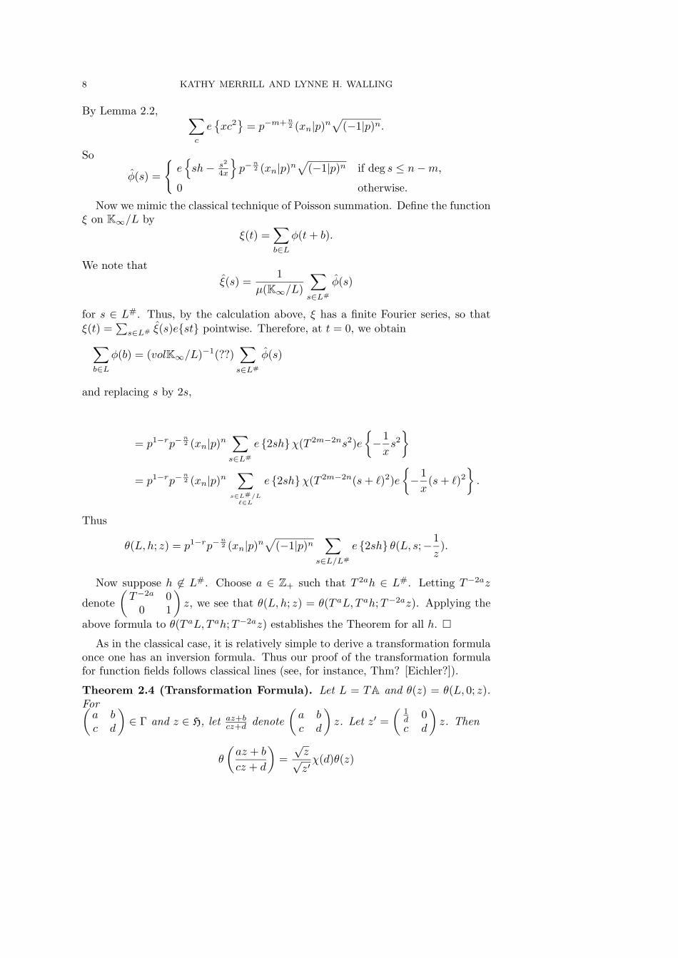
As in the classical case, it is relatively simple to derive a transformation formulaonce one has an inversion formula. Thus our proof of the transformation formulafor function fields follows classical lines (see, for instance, Thm? [Eichler?]).

Theorem 2.4 (Transformation Formula). Let L = TA and θ(z) = θ(L, 0; z).For(a bc d

)∈ Γ and z ∈ H, let az+b

cz+d denote(a bc d

)z. Let z′ =

(1d 0c d

)z. Then

θ

(az + b

cz + d

)=√z√z′χ(d)θ(z)


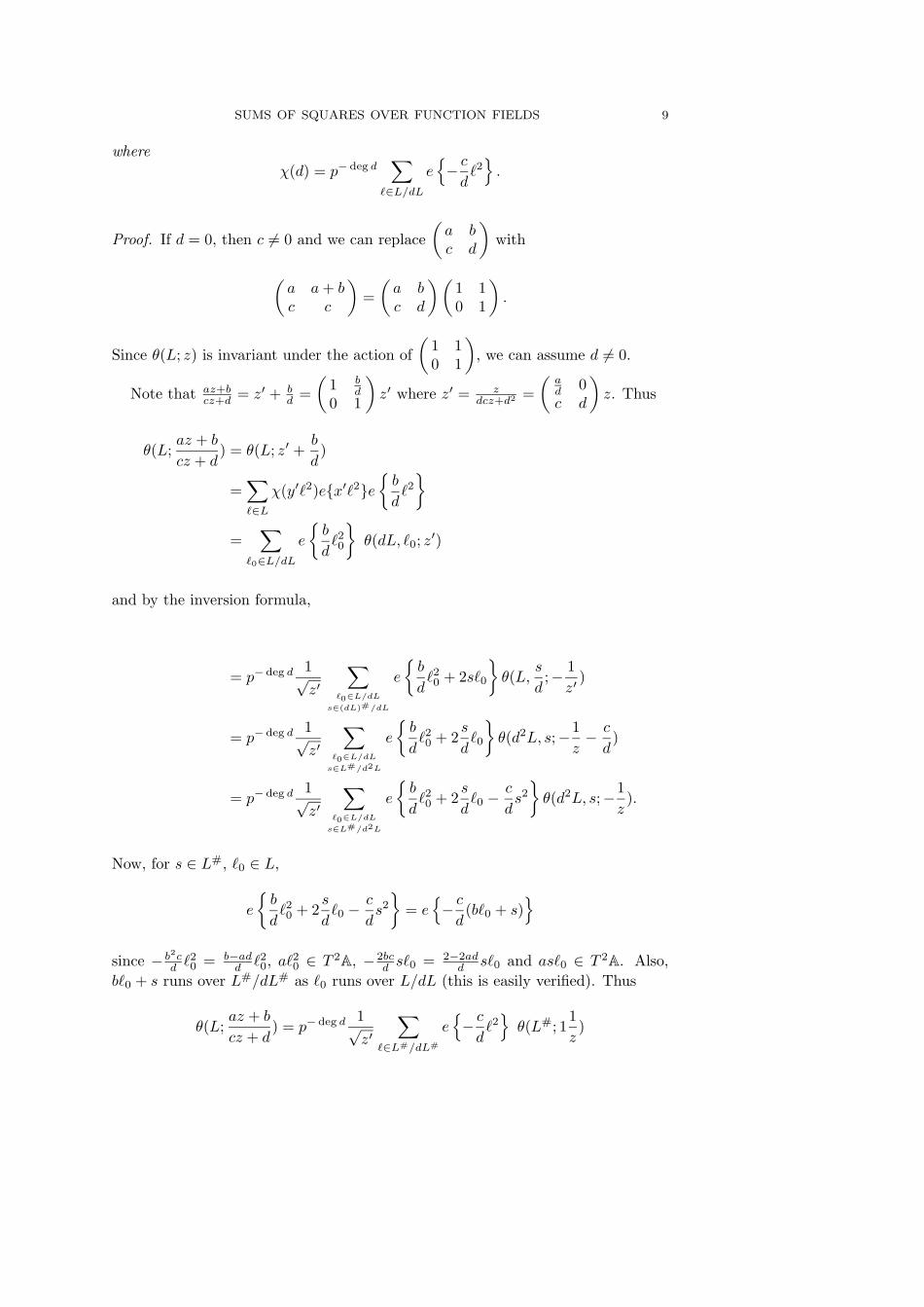
whereχ(d) = p− deg d

∑`∈L/dL

e{− cd`2}.

Proof. If d = 0, then c 6= 0 and we can replace(a bc d

)with

(a a+ bc c

)=(a bc d

)(1 10 1

).

Since θ(L; z) is invariant under the action of(

1 10 1

), we can assume d 6= 0.

Note that az+bcz+d = z′ + b

d =(

1 bd

0 1

)z′ where z′ = z

dcz+d2 =(ad 0c d

)z. Thus

θ(L;az + b

cz + d) = θ(L; z′ +

b

d)

=∑`∈L

χ(y′`2)e{x′`2}e{b

d`2}

=∑

`0∈L/dL

e

{b

d`20

}θ(dL, `0; z′)

and by the inversion formula,

= p− deg d 1√z′

∑`0∈L/dL

s∈(dL)#/dL

e

{b

d`20 + 2s`0

}θ(L,

s

d;− 1

z′)


∑`0∈L/dLs∈L#/d2L

e

{b

d`20 + 2

s

d`0

}θ(d2L, s;−1

z− c

d)


∑`0∈L/dLs∈L#/d2L

e

{b

d`20 + 2

s

d`0 −

c

ds2

}θ(d2L, s;−1

z).

Now, for s ∈ L#, `0 ∈ L,

e

{b

d`20 + 2

s

d`0 −

c

ds2

}= e

{− cd

(b`0 + s)}

since − b2cd `

20 = b−ad

d `20, a`20 ∈ T 2A, − 2bc

d s`0 = 2−2add s`0 and as`0 ∈ T 2

A. Also,b`0 + s runs over L#/dL# as `0 runs over L/dL (this is easily verified). Thus

θ(L;az + b

cz + d) = p− deg d 1√

z′

∑`∈L#/dL#

e{− cd`2}θ(L#; 1

1z

)


and again by the inversion formula,

= p− deg d

√z√z′

∑`∈L/dL

e{− cd`2}θ(L; z)

(recall that we have chosen L so that L# = L). �

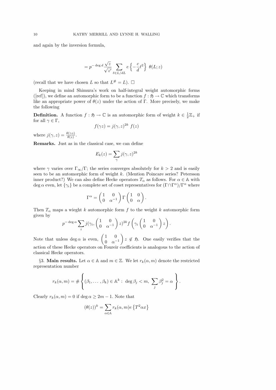
Keeping in mind Shimura’s work on half-integral weight automorphic forms([ref]), we define an automorphic form to be a function f : H→ C which transformslike an appropriate power of θ(z) under the action of Γ. More precisely, we makethe following

Definition. A function f : H → C is an automorphic form of weight k ∈ 12Z+ if

for all γ ∈ Γ,f(γz) = j(γ, z)2k f(z)

where j(γ, z) = θ(γz)θ(z) .

Remarks. Just as in the classical case, we can define

Ek(z) =∑γ

j(γ, z)2k

where γ varies over Γ∞/Γ; the series converges absolutely for k > 2 and is easilyseen to be an automorphic form of weight k. (Mention Poincare series? Peterssoninner product?) We can also define Hecke operators Tα as follows. For α ∈ A withdegα even, let {γi} be a complete set of coset representatives for (Γ∩Γα)/Γα where

Γα =(

1 00 α−1

)Γ(

1 00 α

).

Then Tα maps a wieght k automorphic form f to the weight k automorphic formgiven by

p− degα∑i

j(γi,(

1 00 α−1

)z)2kf

(γi

(1 00 α−1

)z

).

Note that unless degα is even,(

1 00 α−1

)z 6∈ H. One easily verifies that the

action of these Hecke operators on Foureir coefficients is analogous to the action ofclassical Hecke operators.

§3. Main results. Let α ∈ A and m ∈ Z. We let rk(α,m) denote the restrictedrepresentation number

rk(α,m) = #

(β1, . . . , βk) ∈ Ak : deg βj < m,∑j

β2j = α

.

Clearly rk(α,m) = 0 if degα ≥ 2m− 1. Note that

(θ(z))k =∑α∈A

rk(α,m)e{T 2αx

}


where z =(T−2m x

0 1

)(that is, rk(α,m) = cT 2α(T−2m)). Thus to study the

representation numbers we will study the automorphic form (θ(z))k. However,since θ(z)k has weight k

2 , we will ease our computations here by only consideringeven powers of θ(z). Thus we fix k ∈ Z+, and we consider the weight k automorphicform θ(z)2k. Also, to ease the notation, let r(α,m) = r2k(α,m).

As we mentioned earlier, we will evenually analyze the Fourier coefficents ofθ(z)2k by anlayzing its behavior on a fundamental domain. To prepare for this wehave

Proposition 3.1.

(1) The set{(

T 2m x0 1

): m ≥ 0, x ∈ T 2m+1

A/A

}is a complete set of coset rep-

resentatives for Γ∞\H.

(2) The set{(

T 2m 00 1

): m ≥ 0

}is a complete set of coset representatives for

Γ\H.

Proof. The proof of (1) is trivial and hence is omitted. The proof of (2) follows

easily from the observations that(

0 −11 0

)and

{(1 a0 1

): a ∈ A

}generate Γ,

and for z =(T−2m x

0 1

)∈ H, x ∈ T 1−2m

A,

−1z

=(

0 −11 0

)z =

(T 2m 0

0 1

)if x = 0,(

T 2n−2m − 1x

0 1

)if x 6= 0, deg x = −n.

�

Next we need the following technical Lemma.

Lemma 3.2. Let d ∈ Z+, u =∑

−d<j≤0

ujTj with u0 6= 0. Write

1u

=∑

−d<j≤0

vjTj + v

where v ∈ Pd∞. Then for 0 ≤ n < d, v−n depends only on u0, u−1, . . . , u−n, and it

is linear in u−n.

Proof. We argue by induction on n. One easily sees that v0 = 1u0

, so assume0 < n < d, and suppose that vj depends only on u0, . . . , uj for −n < j ≤ 0. Set

u′ =∑

−n<j≤0

ujTj , and v′ =

∑−n<j≤0

vjTj .

Then u = u′ + u−nT−n + u′′, and 1

u = v′ + v−nT−n + v′′ where u′′, v′′ ∈ Pn+1

∞ .Thus

1 = u′v′ + (u0v−D + v0u−n)T−n + w


where w ∈ Pn+1∞ . So v−n = − 1

u0(v0u−n + [u′v′]−n) where [u′v′]−n denotes the

coefficient of T−n in the expansion of u′v′. By hypothesis, v′ depends only onu0, . . . , u1−n; thus v−n depends only on u0, . . . , u−n and is linear in u−n. �

With this we get our preliminary description of the 0th Fourier coefficients, orequivalently, the number of ways to represent 0 as a sum of 2k squares.

Proposition 3.3. For m ∈ Z+,

r(0,m) = p2m(k−1)+1 + (p− 1)∑

1≤n<2m

pn(k−1)(−1|p)nkr(0,m− n).

Proof. We show that

c0(T−2m) = p2m(k−1)+1 + (p− 1)∑

1≤n<2m

pn(k−1)(−1|p)nkc0(T 2n−2m).

We know from Theorem 1.3 that

p2m−1c0(T−2m)

=∑

x∈T 1−2mA/A

f

((T−2m x

0 1

))

= f

((T−2m 0

0 1

))+

∑1≤n<2m

∑u∈(O∞/P2m−n

∞ )×f

((T−2m T−nu

0 1

))

and applying the inversion formula (Theorem 2.3),

= p2mkf

((T 2m 0

0 1

))+

∑1≤n<2m

pnk(−1|p)nk∑

u∈(O∞/P2m−n∞ )×

f

((T 2n−2m Tn 1

u0 1

)).

We know that f((

T 2m 00 1

))= c0(T 2m) = 1; similarly, for m ≤ n < 2m,

f

((T 2n−2m ∗

0 1

))= c0(T 2n−2m) = 1.

Note that(O∞/P2m−n

∞)× has (p− 1)p2m−n−1 elements. Thus

p2m−1c0(T−2m) = p2mkc0(T 2m)

+ p2m−1(p− 1)∑

m≤n<2m

pn(k−1)(−1|p)nkc0(T 2n−2m)

+∑

1≤n<m

∑u

f

((T 2n−2m Tn 1

u0 1

)).


If m = 1 then we are done. So suppose m > 1, and fix n, 1 ≤ n < m, and chooseu ∈

(O∞/P2m−n

∞)×. From the previous Lemma we know that 1

u

∑j ujT

j where,for n − 2m < j ≤ −1, u−j is dependent only on u0, . . . , uj and it is linear in uj .Recalling that f is invariant under the left action of Γ∞ and the right action ofPSL2(O∞), we see that

f

((T 2n−2m Tn 1

u0 1

))= f

((T 2n−2m v

0 1

))

with v =∑

2n−2m<j<0

uj+nTj . As u varies over

(O∞/P2m−n

∞)×, the preceding

Lemma implies that the corresponding v are evenly distributed over P∞/P2m−2n∞ .

Thus

p2m−1c0(T−2m)

= p2mk + p2m−1(p− 1)∑

m≤n<2m

pn(k−1)(−1|p)nkc0(T 2n−2m)

+∑

1≤n<m

pnk(−1|P )nk(p− 1)pn∑

v∈P∞/P2n−2m∞

f

((T 2n−2m v

0 1

)).

Now, Theorem 1.3 shows that

∑v∈P∞/P

2n−2m∞

f

((T 2n−2m v

0 1

))=

∑v∈TA/T 1+2n−2mA

f

((T 2n−2m v

0 1

))= p2m−2n−1c0(T 2n−2m),

and the Theorem now follows. �

Our next goal is to describe the representation numbers in closed form. Onceagain, we first need a Lemma.

Lemma 3.4. For m ≥ 1,

r(0,m) = (−1|p)kpkr(0,m− 1) + p2m(k−1)+1 − (−1|p)kp(2m−1)(k−1).

Proof. We use induction on m to show that

c0(T−2m) = (−1|p)kpkc0(T−2(m−1)) + p2m(k−1)+1 − (−1|p)kp(2m−1)(k−1).

Recall that by Proposition 3.3,

c0(T−2m) = p2m(k−1)+1 + (p− 1)∑

1≤n<2m

pn(k−1)(−1|p)nkc0(T 2n−2m).

Case m = 1 of the Lemma follows by noting that p2(k−1)+1 +(p−1)p(k−1)(−1|p)k =(−1|p)kpk + p2(k−1)+1 − (−1|p)kp(k−1). Now assume the statement of the Lemma


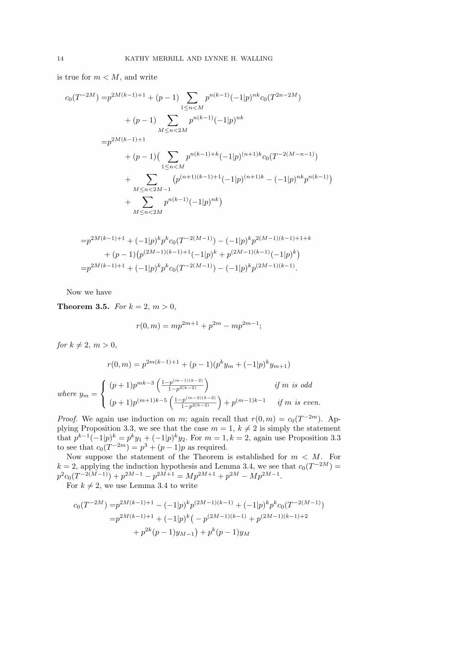
is true for m < M , and write

c0(T−2M ) =p2M(k−1)+1 + (p− 1)∑

1≤n<M

pn(k−1)(−1|p)nkc0(T 2n−2M )

+ (p− 1)∑

M≤n<2M

pn(k−1)(−1|p)nk

=p2M(k−1)+1

+ (p− 1)( ∑

1≤n<M

pn(k−1)+k(−1|p)(n+1)kc0(T−2(M−n−1))

+∑

M≤n<2M−1

(p(n+1)(k−1)+1(−1|p)(n+1)k − (−1|p)nkpn(k−1)

)+

∑M≤n<2M

pn(k−1)(−1|p)nk)

=p2M(k−1)+1 + (−1|p)kpkc0(T−2(M−1))− (−1|p)kp2(M−1)(k−1)+1+k

+ (p− 1)(p(2M−1)(k−1)+1(−1|p)k + p(2M−1)(k−1)(−1|p)k

)=p2M(k−1)+1 + (−1|p)kpkc0(T−2(M−1))− (−1|p)kp(2M−1)(k−1). �

Now we have

Theorem 3.5. For k = 2, m > 0,

r(0,m) = mp2m+1 + p2m −mp2m−1;

for k 6= 2, m > 0,

r(0,m) = p2m(k−1)+1 + (p− 1)(pkym + (−1|p)kym+1)

where ym =

(p+ 1)pmk−3(

1−p(m−1)(k−2)

1−p2(k−2)

)if m is odd

(p+ 1)p(m+1)k−5(

1−p(m−2)(k−2)

1−p2(k−2)

)+ p(m−1)k−1 if m is even.

Proof. We again use induction on m; again recall that r(0,m) = c0(T−2m). Ap-plying Proposition 3.3, we see that the case m = 1, k 6= 2 is simply the statementthat pk−1(−1|p)k = pky1 + (−1|p)ky2. For m = 1, k = 2, again use Proposition 3.3to see that c0(T−2m) = p3 + (p− 1)p as required.

Now suppose the statement of the Theorem is established for m < M . Fork = 2, applying the induction hypothesis and Lemma 3.4, we see that c0(T−2M ) =p2c0(T−2(M−1)) + p2M−1 − p2M+1 = Mp2M+1 + p2M −Mp2M−1.

For k 6= 2, we use Lemma 3.4 to write

c0(T−2M ) =p2M(k−1)+1 − (−1|p)kp(2M−1)(k−1) + (−1|p)kpkc0(T−2(M−1))

=p2M(k−1)+1 + (−1|p)k(− p(2M−1)(k−1) + p(2M−1)(k−1)+2

+ p2k(p− 1)yM−1

)+ pk(p− 1)yM


The Theorem follows by checking that our definitions for yM satisfy yM+1 =p2kyM−1 + (p+ 1)p(2M−1)(k−1). �

Next, we want to describe the restricted representation number r(α,m) whereα ∈ A is nonzero. As when α = 0, we first find a recursive formula. Unfortunately,when degα > 3, this formula involves Kloosterman sums (which we define shortly).Still, this formula leads to a simple description of the average number of ways torepresent a polynomial of fixed degree, and we are able to describe the behavior ofr(α,m) as k →∞, as m→∞, or as degα→∞ (see Theorems 3.11, 3.14, 3.15).

We now need two simple Lemmas.

Lemma 3.6. Let α ∈ K∞, d ∈ Z+ such that D = degα ≤ d. Then

∑u∈(O∞/Pd

∞)×

e {αu} =

(p− 1)pd−1 if α ∈ O∞,−pd−1 if D = 1,0 if D > 1.

Proof. First suppose α ∈ O∞. Then e {αu} = 1 for all u ∈ O∞, so∑u e {αu} is

equal to the cardinality of(O∞/Pd

∞)×.

Next, suppose D = 1. So α = α1T + α′, α′ ∈ O, and∑u

e {αu} =∑u

e {α1Tu}

=∑u

e {α1u0T}

= pd−1∑u0∈F×

e {α1u0T}

= −pd−1.

Finally, suppose D > 1. So α = αDTD + · · ·+ α1T + α′, α′ ∈ O∞. Thus∑

u

e {αu} =∑

u′∈(O∞/PD−1∞ )×

u′′∈PD−1∞ /Pd

e {α(u′ + u′′)}

=∑u′

e {αu′} pd−D∑

u1−D∈F

e {αDu1−DT}

= 0

since the sum on u1−D is a nontrivial character sum. �

Let d ∈ Z+, α, β ∈ K∞ such that degα, deg β ≤ d. Then we define the Kloost-erman sum K(α, β; Pd

∞) by

K(α, β; Pd∞) =

∑u∈(O∞/Pd

∞)×

e

{αu+

β

u

}.

Since degα, deg β ≤ d, the sum on u is well-defined. Notice that u 7→ 1u is an

automorphism of(O∞/Pd

∞)×, so K(α, β; Pd

∞) = K(β, α; Pd∞). Also note that if

α−α′ ∈ O∞ then K(α′, β; Pd∞) = K(α, β; Pd

∞), and if d ≥ D = max {degα, deg β}then

K(α, β; Pd∞) = pd−DK(α, β; PD

∞)

(since e{αw + β

w

}= 1 for w ∈ PD

∞).


Lemma 3.7. Let α, β ∈ K∞ and d ∈ Z+ such that deg β ≤ degα ≤ d. Then

K(α, β; Pd∞) =

(p− 1)pd−1 if α, β ∈ O∞,−pd−1 if β ∈ O∞, degα = 1,0 if degα > 1, degα 6= deg β.

Proof. If β ∈ O∞ thenK(α, β; Pd∞) =

∑u∈(O∞/Pd

∞)× e {αu}, so the Lemma followsfrom the preceding Lemma. So suppose β 6∈ O∞ and D = degα > deg β. Thenα = αDT

D + · · ·+ α1T + v and β = βD−1TD−1 + · · ·+ β1T + w where v, w ∈ O∞

and αD 6= 0. So

K(α, β; Pd∞) =

∑u0,... ,u1−d

e {T (αDu1−D + · · ·+ α1u0 + βD−1u2−D + · · ·+ β1u0)} ;

here u0, . . . , u1−d vary over F, u0 6= 0, and 1u =

∑j ujT

j . We know that u0, . . . , u2−Dare independent of u1−D. Hence we can isolate the sum on u1−D; since αD 6= 0,we have a nontrivial character sum. So K(α, β; Pd

∞) = 0 in this case. �

Now we obtain our preliminary description of r(α,m) for α 6= 0.

Proposition 3.8. Take α ∈ A, α 6= 0; let D = degα and fix m ∈ Z+ such thatD < 2m− 1. Then

r(α,m)

= p ·∑

D+1<n≤2m

pn(k−1)(−1|p)nkr(0,m− n)

−∑

D+1≤n<2m

pn(k−1)(−1|p)nkr(0,m− n)

+∑

1≤n≤D2

pnk(−1|p)nk∑β∈A

deg β=D−2n

r(β,m− n)p−D−2K(αT 2−n, βT 2+n; PD+2−n∞ ).

Proof. We prove the analogous formula for cT 2α(T−2m). Take α ∈ T 2A, α 6= 0; let

D = degα. Fix m ∈ Z+ such that D ≤ 2m. Recall that with z =(T−2m x

0 1

),

we have

−1z

=

(T 2m 0

0 1

)if x = 0,(

T 2n−2m − 1x

0 1

)if x 6= 0, −n = deg x > −2m.

Also note that T−nu + A runs over the nonzero elements of T 2m+1A/A as n and

u vary, 1 ≤ n < 2m, u ∈(O∞/P2m−n

∞)×. Thus the Fourier transform and the

inversion formula give us

p2m−1cα(T−2m)

= p2mkf

((T 2m 0

0 1

))+

∑1≤n<2m

pnk(−1|p)nk∑

u∈(O∞/P2m−n∞ )×

f

((T 2n−2m Tn 1

u0 1

))e{αT−nu

}


and since f((

T 2n−2m ∗0 1

))= c0(T 2n−2m) = 1 when n ≥ m,

= p2mk +∑

m≤n<2m

pnk(−1|p)nkc0(T 2n−2m) ·∑

u∈(O∞/P2m−n∞ )×

e{αT−nu

}+

∑1≤n<m

pnk(−1|p)nk∑

u∈(O∞/P2m−n∞ )×

β∈T2A

cβ(T 2n−2m)e{αT−nu+ βTn/u

}.

Now by Lemma 3.7 and Proposition 3.8, this is equal to

p2mk +∑

D≤n<2m

pnk(−1|p)nk(p− 1)p2m−n−1c0(T 2n−2m)

− p(D−1)k(−1|p)(D−1)kp2m−Dc0(T 2n−2m)

+∑

1≤n<mdeg β=D−2n

pnk(−1|p)nkcβ(T 2n−2m)K(αT−n, βTn; P2m−n∞ ).

Finally, we recall that since degαT−n = deg βTn = D−n, K(αT−n, βTn; P2m−n∞ ) =

p2m−DK(αT−n, βTn; PD−n∞ ).�

Next we remove some of the recursion for our formula for r(α,m) by analyzingwhat we consider the main term.

Theorem 3.9. Suppose α ∈ A is nonzero with degα = D < 2m− 1. Write

r(α,m) = gD,m+∑

1≤n≤D2deg β=D−2n

pnk(−1|p)nkr(β,m−n)p−D−2K(αT 2−n, βT 2+n; PD+2−n∞ ).

If k = 1, we have

gD,m =( [D + 2

2

]p−

[D + 1

2

] )+ (−1|p)

( [D + 12

]p−

[D + 2

2

] ).

If k 6= 1, then

gD,m = p2m(k−1)+1 + sD,m + (−1|p)kpk−1sD+1,m

where sD,m =

(p− 1)p(2m−D)(k−1) (1−p(k−1)D)1−p2(k−1) if D is even

(p− 1)p(2m−D+1)(k−1) (1−p(k−1)(D−1))(1−p2(k−1))

− p(2m−D−1)(k−1) if D is odd.

Proof. Again, we prove the analogous formula for cα(T−2m) where α ∈ T 2A,α 6= 0,

and D = degα. From Proposition 3.8, we know that

gD,m =p2m(k−1)+1 +∑

D≤n<2m

pn(k−1)(−1|p)nk(p− 1)c0(T 2n−2m)

− p(D−1)(k−1)(−1|p)(D−1)kc0(T 2(D−1)−2m)

=c0(T−2m)−∑

1≤n<D

pn(k−1)(−1|p)nk(p− 1)c0(T 2n−2m)

− p(D−1)(k−1)(−1|p)(D−1)kc0(T 2(D−1)−2m)


We will use induction on D and Lemma 3.4 to show that g(2m) has the requiredform. If D = 2, we see that

g(2m) = c0(T−2m)− pk(−1|p)kc0(T−2m+2) = p2m(k−1)+1 − (−1|p)kp(2m−1)(k−1).

If k = 1, this reduces to p− (−1|p).Now we assume that the statement of the Theorem is true for D < d, and note

that if gD,m is associated with an α of degree d-1 while gd,m is associated with anα′ of degree d, then

gd,m =gD,m + p(d−2)(k−1)(−1|p)(d−2)kc0(T−2(m−d+2))

− p(d−1)(k−1)+1(−1|p)(d−1)kc0(T−2(m−d+1)

=gD,m + p(d−2)(k−1)(−1|p)(d−2)k(p(2m−2d+4)(k−1)+1

− (−1|p)kp(2m−2d+3)(k−1))

In the case k = 1, the induction hypothesis then shows that

gd,m =( [d− 1

2

]p−

[d− 2

2

] )+ (−1|p)

( [d− 22

]p−

[d− 1

2

] )+ (−1|p)d(p− (−1|p))

=( [d

2

]p−

[d− 1

2

] )+ (−1|p)

( [d− 12

]p−

[d

2

] ).

If k 6= 1,

g′(2m)

={sd−1,m + p(2m−d+2)(k−1)+1 + (−1|p)k(pk−1sd,m − p(2m−d+1)(k−1)) if d is even,

sd−1,m + p(2m−d+1)(k−1) + (−1|p)k(pk−1sd,m + p(2m−d+2)(k−1)+1) if d is odd.

It will suffice to show that our formulas for sd,m satisfy

sd,m ={sd−1,m + p(2m−d+2)(k−1) if d is even,

sd−1,m − p(2m−d+1)(k−1) if d is odd.

This is easily verified. �

We consider here a few special cases.

Corollary 3.10. For α ∈ A, let Rα denote the number of distinct nonzero rootsof α which lie in F; let g(2m) be as in the preceding Theorem.

(1) Suppose α ∈ A with degα = 0 or 1. Then for m ∈ Z+ with D = degα < 2m−1,r(α,m) = g(2m).

(2) Suppose α ∈ A has degree 2. Then for m ∈ Z+ with m ≥ 2,

r(α,m) = g2,m + (−1|p)kg0,mpk−3(pRα − p+ 1).

(3) Suppose α ∈ A has degree 3. Then for m ∈ Z+ with m ≥ 3,

r(α,m) = g3,m + (−1|p)kg1,mpk−4(pRα − p+ 1).


CHECK THESE FOR SMALL M?

Proof. Recall that r(α,m) = cT 2α(T−2m); thus we analyze cα(T−2m) where α ∈T 2A has degree 4 or 5.(1) This follows immediately from the preceding Theorem.(2) First suppose α, β ∈ T 2

A with degα = 4 and deg β = 2. Then for u =∑j ujT

j ∈ O×∞, we have

1u

=1u0− u−1

u20

T−1 +u2−1 − u0u−2

u30

T−2 + w

where w ∈ P3∞. Thus

K(αT−1, βT ; P3∞)

=∑

u0,u−1,u−2

e

{T (α4u−2 + α3u−1 + α2u0 + β2

u2−1 − u0u−2

u30

)}.

Isolating the sum on u−2, we have a character sum which yields 0 except whenβ2 = u2

0α4. So K(αT−1, βT ; P3∞) = 0 unless (β2|p) = (α4|p). Suppose we have

(β2|p) = (α4|p); then β2 = v20α4 = (−v0)2α4 for some v0 ∈ F×, and

K(αT−1, βT ; P3∞) = p

∑u−1∈F

e

{T (α4

u2−1

vo+ α3u−1 + α2v0)

}

+ p∑u−1∈F

e

{T (−α4

u2−1

v0+ α3u−1 − α2v0)

}

and replacing u−1 by v0u−1 in the first sum and by −v0u−1 in the second sum,

= p∑u−1

e{Tv0(α4u

2−1 + α3u−1 + α2)

}+ p

∑u−1

e{−Tv0(α4u

2−1 + α3u−1 + α2)

}.

Now we sum over β ∈ T 2A, deg β = 2. (Note that r(β,m − 1) = g0,m−1 since

deg β = 1.) So this means we vary v20 over F×. Thus we have∑

β∈T2Adeg β=2

K(αT−1, βT ; P3∞)

= p∑

u−1∈F×

v0∈F×

e{Tv0(α4u

2−1 + α3u−1 + α2)

}.

The sum on v0 is equal to p − 1 if u−1 is a root of α2 + α3T + α4T2, and −1

otherwise. Thus ∑β

K(αT−1, βT ; P3∞) = p(pRα − p+ 1).


The result now follows from the preceding Theorem.(3) Now let α = α5T

5 + α4T4 + α3T

3 + α2T2 and β = β3T

3 + β2T2. For

u =∑j ujT

j ∈ O×∞, we have

1u

=1u0− u−1

u20

T−1 +u2−1 − u0u−2

u30

T−2 +2u0u−1u−2 − u3

−1 − u20u−2

u40

T−3 + w

where w ∈ P4∞. So

K(αT−1, βT ; P4∞)

=∑

u0,... ,u−3

e {T (α5u−3 + α4u−2 + α3u−1 + α2u0}

· e{β3

2u0u−1u−2 − u3−1 − u2

0u−2

u40

+ β2u2−1 − u0u−2

u30

)}.

The sum on u−3 is 0 if β3 6= u20α5, and p otherwise. So suppose β3 = v2

0α5 =(−v0)2α5 for some v0 ∈ F×. Then

K(αT−n, βTn; P4∞)

= p∑u−1

e

{T (α3u−1 + α2v0 −

α5u3−1

v20

+β2u

2−1

v30

)}

·∑u−2

e

{Tu−2(α4 +

2α5u−1

v0− β2

v20

)}

and since the sum on u−2 is a character sum,

= p2∑u−1

e

{T (α2v0 + α3u−1 +

α4u2−1

v0+α5u

3−1

v20

)}

+ p2∑u−1

e

{T (−α2v0 + α3u−1 −

α4u2−1

v0+α5u

3−1

v20

)}

and replacing u−1 by v0u−1 in the first sum and by −v0u−1 in the second sum,

= p2∑u−1

e{Tv0(α2 + α3u−1 + α4u

2−1 + α5u

3−1)}

+ p2∑u−1

e{−Tv0(α2 + α3u−1 + α4u

2−1 + α5u

3−1)}.

Now we sum over β, so we need to vary v20 . (Note that r(β,m− 1) = g1,m−1 since

deg β = 1.) Thus we have

K(αT−n, βTn; P4∞) =

∑u−1∈Fv0∈F×

e{Tv0(α2 + α3u−1 + α4u

2−1 + α5u

3−1)}.


The sum on v0 yields p− 1 if u−1 is a root of T−2α, and −1 otherwise. So we get∑β

K(αT−1, βT ; P4∞) = p2(pRα + p− 1).

The result now follows from the preceding Theorem. �

This corollary suggests that the values of the sums of Kloosterman sums whichappear in the formula in Theorem 2.9 vary wildly(?), depending on the factorizationof α over F. At present we are unable to analyze these sums of Kloosterman sumsexcept in the cases treated above. However, we are able to determine the averagevalue of these sums as we vary α as described in the next Theorem. We thankDavid Grant for suggesting this result.

Theorem 3.11. Fix D,m ∈ Z+ such that D < 2m−1. For α ∈ A with degα = D,write α = α0 + · · · + αDT

D. Choose t ∈ Z such that[D2

]≤ t ≤ D. Then, varying

the coefficients α0, . . . , αt over F, the average value of r(α,m) is

r(α,m) = gD,m.

Proof. We know r(α,m) = cT 2α(T−2m); thus by Theorem 3.9 it suffices to showthat for any n, 1 ≤ n ≤ D

2 + 1 and β ∈ T 2A such that deg β = D + 2− 2n,∑

α1,... ,αt

K(αT 2−n, βTn; PD+2−n∞ ) = 0.

Note that the preceding corollary imples the Theorem holds for D = 0 or 1, so wemay assume here that D > 1. Since

[D2

]≤ t ≤ D, αn−1 varies over F; hence∑

α1,... ,αt

K(αT 2−n, βTn; PD+2−n∞ )

=∑u, αjj 6=n−1

e

{βTn

u+ (α− αn−1T

n−1)T 2−nu

} ∑αn−1

e {αn−1u0T}

where u =∑j ujT

j ∈(O∞/PD−n

∞)×, αj ∈ F (and αD 6= 0). Since u0 6= 0, the sum

on αn−1 is a nontrivial character sum. �

Despite our poor understanding of sums of Kloosterman sums, Theorem 3.9does allow us to determine the order of magnitude of r(α,m) as m → ∞ or asdegα→∞, as well as an asymptotic formula for r(α,m) as k →∞. To obtain thefirst of these results, we need to find a bound for each sum of Kloosterman sums.Thus we have

Lemma 3.12. Fix α ∈ T 2A such that degα = D ≥ 4, and fix n, 1 ≤ n ≤ D

2 − 1.Then ∣∣∣∣∣∣∣

∑β∈T2A

deg β=D−2n

K(αT−n, βTn; PD−n∞ )

∣∣∣∣∣∣∣ < pD−n.


Proof. By definition,∑β


=∑β

∑u∈(O∞/PD−n

∞ )×e

{αT−n

u+ βTnu

}

=∑

β2,... ,βD−2nu0,... ,u1+n−D

e {T (αDu1+n−D + · · ·+ α1+nu0 + βD−2nu1+n−D + · · ·+ β2u−n−1)} ;

here βD−2n 6= 0, u0 6= 0, and 1u =

∑j ujT

j . As βj varies over F, 2 ≤ j ≤ D − 2n,we get a character sum on βj . So whenever uj 6= 0, 2 ≤ j ≤ D − 2n, the sum onthe βj becomes 0. Thus we are left with a sum on u0, . . . , u−n and on u1+n−D;this sum has (p− 1)p1+n terms. Hence∣∣∣∣∣∣

∑β


∣∣∣∣∣∣ < pD−n.

�

Lemma 3.13. Let gD,m be as in Theorem 3.9. Then

gD,m = p2m(k−1)+1 + tD,m

where |tD,m| < 2p(2m02)(k−1)+1(1 + pk−1).

Proof. We know from Theorem 3.9 that

gD,m = p2m(k−1)+1 + sD,m + (−1|p)kpk−1sD+1,m.

Now,

sD+1,m

=

(p− 1)p(2m−D+1)(k−1)(p(D−3)(k−1) + p(D−5)(k−1) + · · ·+ 1)if D is odd,

(p− 1)p(2m−D+2)(k−1)(p(D−4)(k−1) + p(D−6)(k−1) + · · ·+ 1)

−p(2m−D)(k−1)

if D is even,

=

(p− 1)p(2m−2)(k−1)(1 + p−2(k−1) + p−4(k−1) + · · ·+ p−(D−3)(k−1))

if D is odd,(p− 1)p(2m−2)(k−1)(1 + p−2(k−1) + p−4(k−1) + · · ·+ p−(D−4)(k−1))

−p(2m−D)(k−1) if D is even.

So |pk−1sD+1,m| < 2p(2m−1)(k−1)+1, and |sD,m| < 2p(2m−2)(k−1)+1. �


Theorem 3.14. For α ∈ A, k > 1, r(α,m) = O(p2m(k−1)) as m → ∞ or asD = degα→∞ (with 2m = D + t, t fixed).

Proof. We show that for α ∈ T 2A, cα(T−2m) = O(p2m(k−1)) as m → ∞ or as

D = degα → ∞. So take α ∈ T 2A. To ease the notation, let Kn(α, β) =

pn−DK(αT−n, βTn; PD−n∞ ) where degα = D and deg β = D − 2n. Then using

Theorem 3.9 repeatedly, we find that

cα(T−2m)

= g(2m) +∑

1≤n1≤D2 −1

deg β(1)=D−2n1

pn1(k−1)(−1|p)n1kcβ(1)(T 2n1−2m)Kn1(α, β(1))

= g(2m)

+∑

1≤n1≤D2 −1

pn1(k−1)(−1|p)n1kg(2m− 2n1)∑

deg β(1)=D−2n1

Kn1(α, β(1))

+∑

1≤n1≤D2 −1

1≤n2≤n1

p(n1+n2)(k−1)(−1|p)(n1+n2)k∑

deg β(2)=D−2n2

cβ(2)(T 2(n1+n2)−2m)

·∑β(1)

Kn1(α, β(1))Kn2(α, β(2))

= g(2m) +∑n1

pn1(k−1)(−1|p)n1kg(2m− 2n1)∑β(1)

Kn1(α, β(1))

+∑n1,n2

p(n1+n2)(k−1)(−1|p)(n1+n2)kg(2m− 2(n1 + n2))

·∑

β(1),β(2)

Kn1(α, β(1))Kn2(β(1), β(2))

+ · · ·+

+∑

n1,... ,nd

p(n1+···+nd)(k−1)(−1|p)(n1+···+nd)kg(2m− 2(n1 + · · ·+ nd))

·∑

β(1),... ,β(d)

Kn1(α, β(1)) · · ·Knd(β(d−1), β(d))

where d =[D2 − 1

]. The previous Lemma shows that the sums on the β(j) are

bounded by 1. Hence

|cα(T−2m)| ≤ |g(2m)|+∑

1≤r≤d

∑n1,... ,nr

p(n1+···+nr)(k−1) |g(2m− 2(n1 + · · ·+ nr))|

where 1 ≤ n1 ≤ D2 − 1 and 1 ≤ nj ≤ D

2 − nj−1 − · · · − n1 − 1 for j > 1. Now, fix n,1 ≤ n ≤ D

2 − 1. Note that if n1 + · · ·+ nr = n for any positive integers nj then wenecessarily satisfy the above inequalities on the nj . Thus, letting ρ be Ramanujan’spartition function, we have

|cα(T−2m)| ≤ |g(2m)|+∑

1≤n≤D2 −1

ρ(n)pn(k−1)|g(2m− 2n)|


and by the two preceding Lemmas,

≤ Bp2m(k−1)

1 +∑

1≤n≤D2 −1

ρ(n)p−n(k−1)

≤ Bp2m(k−1)

1 +∑1≤n

ρ(n)p−n(k−1)

.

Now, Ramanujan showed (formula 8.3.3, p. 114, [Hardy]) that there is a nonzeroconstant B such that ρ(n) < eB

√n. Thus the series∑

1≤n

ρ(n)p−n(k−1)

converges, and the Theorem is proved. �

Theorem 3.15. Take α ∈ A, α 6= 0; choose m ∈ Z+ such that degα < 2m − 1.Then as k →∞,

r(α,m) = p2m(k−1)+1 +O(p(2m−1)k).

Proof. Take α ∈ T 2A; we show cα(T−2m) = p2m(k−1)+1 + O(p(2m−1)k) as k → ∞.

For degα ≤ 2, the Theorem follows from Corollary 3.10 and Lemma 3.13. We arguenow by induction on D. Suppose D > 2, and suppose for all β ∈ T 2

A, deg β < D,we have cβ(T−2m) = p2m(k−1)+1 +O(p(2m−1)k). We know

cα(T−2m) = p2m(k−1)+1 + p∑

D≤n<2m

pn(k−1)(−1|p)nkc0(T 2n−2m)

−∑

D−1≤n<2m

pn(k−1)(−1|p)nkc0(T 2n−2m)

+∑

1≤n≤D2 −1deg β=D−2n

pn(k−1)(−1|p)nkcβ(T 2n−2m)pn−DK(αT−n, βTn; PD−n∞ ).

We know c0(T 2n−2m) = O(p(2m−2n)k), so pn(k−1)(−1|p)nkc0(T 2n−2m) = O(p(2m−n)k).Similarly, pn(k−1)(−1|p)nkcβ(T 2n−2m) = O(p(2m−n)k) for β ∈ T 2

A of degree D−2n.Now, every Kloosterman sum has pD−n summands, each of modulus 1. Hence wecertainly have

|pn−DK(αT−n, βTn; PD−n∞ )| ≤ 1.

Also, the number of terms in each sum depends only on D and m; in particular,the number of terms in the above sums is independent of k. Thus

cα(T−2m) = p2m(k−1)+1 +∑

D−1≤n<2m

O(p(2m−n)k)

+∑

1≤n≤D2 −1

O(p(2m−n)k)

= p2m(k−1)+1 +O(p(2m−1)k).


�

[Need to add references.]

Department of Mathematics, The Colorado College, Colorado Springs, Col-

orado (zip?)

Department of Mathematics, University of Colorado, Boulder, Colorado 80309-

0395?

sums of squares over function fields kathy merrill and

Documents