Sums of squares of the Littlewood-Richardsoncoefficients and GLn-harmonic polynomials

Pamela E. Harris and Jeb F. Willenbring

Abstract We consider the example from invariant theory concerning the conjuga-tion action of the general linear group on several copies of the n× n matrices, andexamine a symmetric function which stably describes the Hilbert series for the in-variant ring with respect to the multigradation by degree. The terms of this Hilbertseries may be described as a sum of squares of Littlewood-Richardson coefficients.A “principal specialization” of the gradation is then related to the Hilbert series ofthe K-invariant subring in the GLn-harmonic polynomials, where K denotes a blockdiagonal embedding of a product of general linear groups. We also consider otherspecializations of this Hilbert series. 1

1 Introduction

We let Fλn denote the finite dimensional irreducible representation of the general lin-

ear group, GLn, (over C) whose highest weight is indexed by the integer partitionλ = (λ1 ≥ λ2 ≥ ·· · ≥ λn) (in standard coordinates). Given a finite sequence of in-teger partitions µ = (µ(1), · · · ,µ(m)), we will let cλ

µ be the multiplicity of Fλn in the

m-fold tensor product Fµ(1)

n ⊗·· ·⊗Fµ(m)

n under the diagonal action of GLn. That is,cλ

µ denotes the Littlewood-Richardson coefficient (see [Ful97, GW09, Mac95]).

Pamela E. HarrisMarquette University, MSCS DepartmentP.O. Box 1881, Milwaukee WI 53201e-mail: pamela.harris@marquette.edu

Jeb F. WillenbringUniversity of Wisconsin-Milwaukee, Dept. of Math. SciencesP.O. Box 0413, Milwaukee, WI 53211e-mail: jw@uwm.edu

1 This research was supported by the National Security Agency grant # H98230-09-0054.

1

2 Pamela E. Harris and Jeb F. Willenbring

We remark that the usual exposition of Littlewood-Richardson coefficients con-cerns the case where m = 2. However, by iterating the Littlewood-Richardson rule(or its equivalents) one obtains several effective combinatorial interpretations of ourcλ

µ .The subject of this exposition concerns some interpretations of the positive in-

teger ∑(cλ

µ

)2where the sum is over certain finite subsets of non-negative integer

partitions. We believe that such sums have under-appreciated combinatorial signifi-cance. For example, one immediately observes the very simple specialization to thecase where µ( j) = (1) for all j = 1, · · · ,m, in which case the sum of squares is m!.More generally, if ν = (ν1 ≥ ·· · ≥ νm ≥ 0) is a partition and µ( j) = (ν j), then cλ

µ isequal to the Kostka number Kλν (ie. the multiplicity of the weight indexed by ν inFλ

n ).Unless otherwise stated, we will only need notation for representations with poly-

nomial matrix coefficients, which are indexed by partitions with non-negative inte-ger components. The sum of the parts of a partition ν will be called the size (de-noted |ν |), while the number of parts will be called the length denoted `(ν). Asusual, we will also write λ ` d to mean |λ | = d. Furthermore, we also adapt the(non-standard) notation that if µ = (µ(1), · · · ,µ(m)) is a finite sequence of partitions,we set |µ| = ∑

mj=1 |µ( j)|, and write µ ` d to mean |µ| = d. From a combinatorial

point of view, the results involve a specialization of the following

Main Formula Let t1, t2, t3, · · · denote a countably infinite set of indeterminates. Wehave

∞

∏k=1

11−(tk1 + tk

2 + tk3 + · · ·

) = ∑λ

∑µ

(cλ

µ

)2tµ

where the outer sum is over all partitions λ and the inner sum is over all finite

sequences of partitions µ = (µ(1),µ(2),µ(3), · · ·) with tµ = t |µ(1)|

1 t |µ(2)|

2 t |µ(3)|

3 · · ·.Proof. See Section 7. ut

As an application of the main formula, we turn to the space, H (gln), of GLn-harmonic polynomial functions on the adjoint representation (with its natural gra-dation) by polynomial degree, H (gln) =

⊕∞d=0 H d(gln). The group GLn acts on

H (gln). Note that the constant functions are the only GLn-invariant harmonic func-tions. However, if K is a reductive subgroup of GLn, the space of K-invariant func-tions is much larger. Consider the example when the group K is the block diagonallyembedded copy of GLn1×·· ·×GLnm in GLn, with n1+ · · ·+nm = n. We will denotethis group by K(n) where n = (n1, · · · ,nm). The purpose of this paper is to relate thedimension of the K(n)-invariant polynomials in H d(gln) to a sum of squares ofLittlewood-Richardson coefficients. See Theorem 1 for the precise statement.

We consider this question because the related algebraic combinatorics are par-ticularly elegant, and hence have expository value in connecting harmonic analysiswith algebraic combinatorics. However, this example is the tip of an iceberg. Indeed,one can replace GLn with any algebraic group G (with g = Lie(G)) and K(n) withany subgroup of G. This area of investigation is wide open and well motivated as anexamination of the special symmetries of harmonic polynomials.

Summing Squares 3

In Section 2, we describe a general “answer” to this question when K is a sym-metric subgroup of a reductive group G. This answer is not as explicit as wouldbe desired, but applies to any symmetric pair (G,K). The remainder of the paperis related to the G = GLn example with K = K(n). Note that when m = 2 (ie.n = (n1,n2)) the pair (G,K) is symmetric, but for m > 2 is not. We remark thatin the m = 2 case, the results presented here were first described in [Wil07]. Ourpresent discussion amounts to a generalization to m > 2.

After setting up appropriate notation in Section 3 we provide an interpretationfor a description of the Hilbert series of the K(n)-invariants in the GLn-harmonicpolynomials on gln in Sections 4 and 5. Chief among these involves sums of squaresof Littlewood-Richardson coefficients. We recall other combinatorial interpretationsin Section 6. These interpretations involve counting the conjugacy classes in thegeneral linear group over a finite field.

2 The case of a symmetric pair

Let G denote a connected reductive linear algebraic group over the complex num-bers and let g be its complex Lie algebra. We have g= z(g)⊕gss, where z(g) denotesthe center of g, while gss = [g,g] denotes the semisimple part of g. A celebrated re-sult of Kostant (see [Kos63]) is that the polynomial functions on g, denoted C[g], area free module over the invariant subalgebra, C[g]G, under the adjoint action. Choosea Cartan subalgebra h of g, and let Φ and W denote the corresponding set of rootsand Weyl group, respectively. Choose a set of positive roots Φ+, and let Φ−=−Φ+

denote the negative roots. Set ρ = 12 ∑α∈Φ+ α . For w ∈W , let l(w) denote the num-

ber of positive roots sent to negative roots by w. Fix an indeterminate t. There existpositive integers e1 ≤ e2 ≤ ·· · ≤ er such that ∑w∈W t l(w) = ∏

rj=1

1−te j

1−t where r isthe rank of gss. A consequence of the Chevalley restriction theorem ([Che55]) isthat C[g]G is freely generated, as a commutative ring, by dimz(g) polynomials ofdegree 1, and r polynomials of degree e1, · · · ,er. These polynomials are the basicinvariants, while e1, · · · ,er are called the exponents of G.

2.1 Harmonic polynomials

We define the harmonic polynomials on g by

Hg ={

f ∈ C[g]|∆( f ) = 0 for all ∆ ∈ D[g]G}

where D[g]G is the space of constant coefficient G-invariant differential operatorson g. In [Kos63], it is shown that as a G-representation Hg is equivalent to theG-representation algebraically induced from the trivial representation of a maximalalgebraic torus, T, in G. Thus, by Frobenius reciprocity the irreducible rational rep-

4 Pamela E. Harris and Jeb F. Willenbring

resentations of G occur with multiplicity equal to the dimension of their zero weightspace. Moreover, as a representation of G, the harmonic polynomials are equivalentto the regular functions on the nilpotent cone in g.

The harmonic polynomials inherit a gradation by degree from C[g]. Set H dg =

Hg∩C[g]d . Thus, Hg =⊕

∞d=0 H d

g . We next consider the distribution of the mul-tiplicity of an irreducible G-representation among the graded components of Hg. Asolution to this problem was originally due to Hesselink [Hes80], which we recallnext.

Let ℘t : h∗→ N denote2 Lusztig’s q-analog of Kostant’s partition function. Thatis ℘t is defined by the equation,

∏α∈Φ+

11− teα

= ∑ξ∈Q(g,h)

℘t(ξ )eξ

where Q(g,h) ⊆ h∗ denotes the lattice defined by the integer span of the roots. Asusual, eξ denotes the corresponding character of T, with Lie(T) = h. As usual, weset ℘(ξ ) = 0 for ξ /∈ Q(g,h).

Let P(g) denote the integral weights corresponding to the pair (g,h). The dom-inant integral weights corresponding to Φ+ will be denoted P+(g). Let L(λ ) de-note the (finite dimensional) irreducible highest weight representation with highestweight λ ∈ P+(g). The multiplicity of L(λ ) in the degree d harmonic polynomials,H d(g), will be denoted by md(λ ). Set mλ (t) = ∑

∞d=0 md(λ )td . Hesselink’s theorem

asserts thatmλ (t) = ∑

w∈W(−1)l(w)

℘t(w(λ +ρ)−ρ).

See [WW00] for a generalization of this result.We remark that the above formula is very difficult to implement in practice. This

is in part due to the fact that the order of W grows exponentially with the Lie algebrarank. Thankfully, only a small number of terms actually contribute to the overallmultiplicity. See [Har11] for a very interesting special case where the number ofcontributed terms is shown to be a Fibonacci number.

2.2 The K-spherical representations of G

Let (G,K) be a symmetric pair. That is, G is a connected reductive linear algebraicgroup over C and K = {g ∈ G|θ(g) = g}, where θ is a regular automorphism of Gof order two. Since K will necessarily be reductive the quotient, G/K is an affinevariety and the C-algebra of regular function C[G/K] is multiplicity free as a rep-resentation of G. This fact follows from the (complexified) Iwasawa decompositionof G. Put another way, there exists S⊆ P+(g) such that for all λ ∈ P+(g) we have

2 As always, N= {0,1,2,3, · · ·}, the non-negative integers.

Summing Squares 5

dimL(λ )K =

{1, λ ∈ S;0, λ 6∈ S.

Note that the subset S may be read off of the data encoded in the Satake dia-gram associated to the pair (G,K). The above fact implies that the Hilbert seriesHt(G,K) = ∑

∞d=0 hdtd with hd = dimH d(g)K has the following formal expression

Ht(G,K) = ∑w∈W

(−1)l(w)

(∑λ∈S

℘t(w(λ +ρ)−ρ)

).

This formula seems rather encouraging. Unfortunately, the inner sum is very diffi-cult to put into a closed form for general w ∈W . This is, in part, a reflection of thefact that the values of ℘t cannot be determined from a “closed form” expression.However, note that w(λ +ρ)−ρ often falls outside of the support of ℘t , and there-fore it may be possible to obtain explicit results along these lines. Moreover, thepoint of this exposition is to advertise that combinatorially elegant expressions mayexist. At least this is the case for the pair (GLn1+n2 ,GLn1 ×GLn2 ), as we shall see.

3 Preliminaries

We let gln denote the complex Lie algebra of n×n matrices with the usual bracket,[X ,Y ] = XY −Y X , for X ,Y ∈ gln. Let Ei j denote the n× n matrix with a 1 in rowi and column j, and a 0 everywhere else. The Cartan subalgebra will be chosen tobe the span of {Eii|1 ≤ i ≤ n}. The dual basis in h∗ to (E11,E22, · · · ,Enn) will bedenoted (ε1, · · · ,εn). Choose the simple roots as usual, Π = {εi− εi+1|1 ≤ i < n}.Let Φ (resp. Φ+) denote the roots (resp. positive roots). We will identify h withh∗ using the trace form, (H1,H2) = Tr(H1H2) (for H1,H2 ∈ h). The fundamentalweights are ωi = ∑

ij=1 ε j ∈ h∗ for 1≤ i≤ n−1. We also set ωn = ∑

nj=1 ε j ∈ h∗. Let

P(GLn) = ∑nj=1Zω j, and P+(GLn) = Zωn +∑

n−1j=1 Nω j.

From this point on, we will write (a1, · · · ,an) for ∑aiεi. Thus, we have λ =(λ1, · · · ,λn) ∈ P+(GLn) iff each λi in an integer and λ1 ≥ ·· · ≥ λn. The finite di-mensional, irreducible representation of GLn with highest weight λ will be denoted(πλ ,Fλ

n ) whereπλ : GLn→ GL(Fλ

n ).

To simply notation will write Fλn for (πλ ,Fλ

n ).Throughout this article, the representations of GLn which we will consider have

polynomial matrix coefficients. Thus the components of the highest weight λ willbe non-negative integers. Therefore, if λ is a (non-negative integer) partition with atmost ` parts (`≤ n), then the n-tuple, (λ1, · · · ,λ`,0, · · · ,0), corresponds to the highestweight of a finite dimensional irreducible representation of GLn (with polynomialmatrix coefficients).

6 Pamela E. Harris and Jeb F. Willenbring

Under the diagonal action, GLn acts on the d-fold tensor product ⊗dCn. Schur-Weyl duality (see [GW09] Chapter 9) asserts that the full commutant to the GLn-action is generated by the symmetric group action defined by permutation of factors.Consequently, one has a multiplicity free decomposition with respect to the jointaction of GLn× Sd . Moreover, if n ≥ d then every irreducible representation of Sdoccurs. The irreducible representation of Sd paired with Fλ

n will be denoted by V λd .

The full decomposition into irreducible GLn×Sd-representation is⊗dCn ∼=

⊕λ

Fλn ⊗V λ

m

where the sum is over all non-negative integer partitions, λ , of size d and lengthat most n. Note that when n = d, then the condition on `(λ ) is automatic. Thus,all irreducible representations of V λ

d occur. In this manner, the highest weights ofGLn-representations provide a parametrization of the Sd-representations.

Littlewood-Richardson coefficients

Let d = (d1, · · · ,dm) denote a tuple of positive integers with d = d1 + · · ·+dm. LetSd denote the subgroup of Sd consisting of permutations that stabilize the sets per-muting the first m1 indices, then the second m2 indices etc. Clearly, we have

Sd ∼= Sd1 ×·· ·×Sdm .

The irreducible representations of Sd are of the form

V (µ) =V µ(1)

d1⊗·· ·⊗V µ(m)

dm

where µ( j) is a partition of size d j. It is well known that if an irreducible represen-tation, V λ

d , of Sd is restricted to Sd then the multiplicity of V (µ) in V λd is given by

the Littlewood-Richardson coefficient cλµ . This fact is a consequence of Schur-Weyl

duality.

4 Invariant polynomials on matrices

A permutation of {1,2, · · · ,m} may be written as a product of disjoint cycles. Thisresult is fundamental to combinatorial properties of the symmetric group, Sm. Keep-ing this elementary fact in mind, let X = (X1,X2, · · · ,Xm) be a list of complex n×nmatrices. Let Tr denote the trace of a matrix and define

Trσ (X) = Tr(Xσ(1)1

Xσ(1)2· · ·X

σ(1)m1) Tr(X

σ(2)1

Xσ(2)2· · ·X

σ(2)m2) · · ·Tr(X

σ(k)1

Xσ(k)2· · ·X

σ(k)mk)

(1)

Summing Squares 7

where σ = (σ(1)1 σ

(1)2 · · ·σ

(1)m1 )(σ

(2)1 σ

(2)2 · · ·σ

(2)m2 ) · · ·(σ

(k)1 σ

(k)2 · · ·σ

(k)mk ) is a permuta-

tion of m = ∑mi written as a product of k disjoint cycles. Observe that the cyclesof σ may be permuted and rotated without changing the permutation. In turn, thefunction Trσ displays these same symmetries.

Chief among the significance of Trσ is the fact that they are invariant under theconjugation action g ·(X1, · · · ,Xm) = (gX1g−1, · · · ,gXmg−1), where g∈GLn. By set-ting some of the components of (X1, · · · ,Xm) equal one defines a polynomial of equaldegree but on fewer than m copies of Mn. Intuitive, this fact may be described byallowing equalities in the components of the cycles of σ . That is to say (formally)we consider σ up to conjugation by Levi subgroup of Sm.

In [Pro76a,Pro76b], C. Procesi described these generators for the algebra of GLn-invariant polynomials, denoted3 C[V ]GLn , on V = Mm

n , and provided a proof thatthese polynomials span the invariants. Hilbert tells us that the ring of invariants mustbe finitely generated. Thus, there must necessarily be algebraic relations amongthis (infinite) set of generators. In light of Procesi’s work, these generators are, bynow, widely understood. However, it is an important and indeed open problem todetermine the algebraic relations among these invariant polynomials for specificvalues of n and m.

In order to precisely quantify the failure of the Trσ being independent, we intro-duce the formal power series An(t) = An(t1, t2, · · · , tm) = ∑an(d)td with 4 the coeffi-cient defined as an(d) = dimC[Mm

n ]GLnd where C[Mm

n ]d = C[Mn⊕·· ·⊕Mn](d1,···,dm)

denotes the homogeneous polynomials of degree di on the ith copy of Mn. The mul-tivariate series, An(t), is called the Hilbert Series of the invariant ring. Except insome simple cases, a closed form for An(t) is not known. Part of the present expo-sition is to point out the rather simple fact that an(d) may be expressed in terms ofthe squares of Littlewood-Richardson coefficients. Furthermore, we prove

Proposition 1. For any natural numbers m and d = (d1, · · · ,dm)

the limit limn→∞ an(d) exists. If we call the limiting value a(d) and set A(t) =∑a(d)td then

A(t) =∞

∏k=1

11− (tk

1 + tk2 + · · ·+ tk

m).

Proof. The polynomial functions on Mn are multiplicity free under the action ofGLn ×GLn given by (g1,g2) f (X) = f (g−1

1 Xg2) for g1,g2 ∈ GLn, X ∈ Mn andf ∈ C[Mn]. The decomposition is a “Peter-Weyl” type, C[Mn] ∼=

⊕(Fλ

n)∗ ⊗ Fλ

n ,where the sum is over all non-negative integer partitions λ with `(λ )≤ n. We haveC[⊕m

i=1Mn]∼=⊗mi=1C[Mn]. Thus

C[Mmn ]∼=

⊕µ(1)

(Fµ(1)

n

)∗⊗Fµ(1)

n

⊗·· ·⊗⊕

µ(m)

(Fµ(m)

n

)∗⊗Fµ(m)

n

3 Here we let Mn denote the complex vector spaces of n×n matrices (with entries from C).4 We will use the notation d = (d1, · · · ,dm), td = td1

1 · · · tdmm .

8 Pamela E. Harris and Jeb F. Willenbring

∼=⊕α,β

∑µ=(µ(1),···,µ(m))

cαµ cβ

µ

(Fαn )∗⊗Fβ

n ,

with respect to the GLn×GLn action on the diagonal of Mmn . Note that in multide-

gree (d1, · · · ,dm) the sum is over all µ with |µ( j)|= d j. If we restrict to the subgroup{(g,g) : g ∈ GLn} of GLn×GLn, we obtain an invariant exactly when α = β . Thedimension of the GLn-invariants in the degree d homogeneous polynomials on Mm

n

is therefore ∑(cλ

µ

)2where the sum is over all µ = (µ(1), · · · ,µ(m)) and λ ` m with

length at most n. The degree d component decomposes into multi-degree compo-nents (d1, · · · ,dm) with d = ∑d j.

If d ≥ n, then the condition that `(λ )≤ n is automatic, and this fact implies thatif cλ

µ 6= 0, then `(µ( j))≤ n for all j. Thus, the dimension of the degree d invariants

in C[Mmn ] is ∑

(cλ

µ

)2where the sum is over all partitions of size d. If we specialize

the main formula so that t j = 0 for j >m then the sums of squares of the Littlewood-Richardson coefficients agree with A(t). ut

For our present purposes, we will specialize the multigradation on the invariantsin C[Mm

n ] to one that is more course. From this process, we can relate the stabilizedHilbert series of the invariants in H [Mn]. This specialization will be the subject ofthe next section.

We now turn to another problem that, we shall see, is surprisingly related. Con-sider the n×n complex matrix

X =

X(1,1) X(1,2) · · · X(1,m)X(2,1) X(2,2) · · · X(2,m)

......

. . ....

X(m,1) X(m,2) · · · X(m,m)

where X(i, j) is an ni×n j complex matrix with n = ∑n j. Define

Trσ (X) =k

∏j=1

Tr(

X(σ( j)1 ,σ

( j)2 )X(σ

( j)2 ,σ

( j)3 )X(σ

( j)3 ,σ

( j)4 ) · · ·X(σ

( j)m j ,σ

( j)1 )).

Let K(n) denote the block diagonal subgroup of GLn of the form

K(n) =

GLn1. . .

GLnm

.The group K(n) acts on Mn by restricting the adjoint action of GLn. The K(n)-invariant subring of C[Mn] (denoted C[Mn]

K(n)) is spanned by Trσ (X). For smallvalues of the parameter space, these expressions are far from linearly independent

Summing Squares 9

(as in the last example). Formally, one cannot help but notice the symbolic mapTrσ 7→ Trσ . We will try next to make a precise statement along these lines.

Define C[Mn]d to be the homogeneous degree d polynomials on Mn, and letC[Mn]

K(n)d denote the K(n)-invariant subspace. Set a(n)(d) = dimC[Mn]

K(n)d , and

A(n)(t) = ∑∞d=0 a(n)(d) td . Analogous to Proposition 1, we have

Proposition 2. For any non-negative integer d, the limit

limn1→∞

limn2→∞

· · · limnm→∞

a(n1,···,nm)(d)

exists. Denote the limiting value a(d) and set A(t) = ∑∞d=0 a(d)td . We have

A(t) =∞

∏k=1

11−m tk

Proof. We begin with the GLn×GLn-decomposition C[Mn] =⊕(

Fλn)∗⊗Fλ

n withrespect to the action in the proof of Proposition 1. The irreducible GLn-representationFλ

n is reducible upon restriction to K(n). The decomposition is given in terms ofLittlewood-Richardson coefficients

Fλn∼=

⊕µ=(µ(1),···,µ(m))

cλµ Fµ(1)

n ⊗·· ·⊗Fµ(m)

n .

Therefore, as a K(n)×K(n)-representation we have

C[Mn]d = ∑µ,ν

(∑λ

cλµ cλ

ν

) (⊗m

j=1Fµ( j)

n j

)∗⊗(⊗m

j=1Fν( j)

n j

)where the sum is over all λ with |λ | = d, `(λ ) ≤ n and `(µ( j)), `(ν( j)) ≤ n j. If werestrict to the diagonally embedded K(n)-subgroup, we obtain an invariant exactlywhen µ = ν . Thus, a(n)(d) = ∑

(cλ

µ

)2, with the appropriate restrictions on λ and µ .

If all n j ≥ d then the condition on the lengths of partitions disappears, and wemay sum over all λ ` d. The result follows by specializing the main formula bysetting t j = t for 1≤ j ≤ m and t j = 0 for j > m. ut

Although we will not need it for our present purposes, it is worth pointing outthat the algebra C[Mn] has a natural Nm gradation defined by the action of the centerof K(n). This multigradation refines the gradation by degree. The limiting multi-graded Hilbert series is the same as that of Proposition 1. Upon specialization tot1 = t2 = · · · = tm = t we obtain the usual gradation by degree (in both situations).The advantage of considering the more refined gradation is that one can considerthe direct limit as m and n go to infinity. This will be relevant in the next section.

10 Pamela E. Harris and Jeb F. Willenbring

5 Harmonic polynomials on matrices

A specific goal of this article is to understand the dimension of the space of degree dhomogeneous K(n)-invariant harmonic polynomials on Mn. With this fact in mind,we observe the following specialization of the product in the main formula. Lett j = t j. Then we obtain:

∞

∏k=1

11− (tk + t2k + t3k + · · ·)

=∞

∏k=1

1

1− tk

1−tk

=∞

∏k=1

1− tk

1−2tk .

For a sequence µ = (µ(1),µ(2), · · ·) set gr(µ) = ∑∞j=1 j|µ( j)|. The equation in the

main formula becomes

∞

∏k=1

1− tk

1−2tk = ∑λ

∑µ

(cλ

µ

)2tgr(µ).

The notation gr is used for the word grade. We explain this choice next. Let C[Mn;d]denote the polynomials functions on the n× n complex matrices together with thegradation defined by d times the usual degree. That is, C[Mn;d1](d2) denotes thedegree d2 homogeneous polynomials, but regarded as the d1d2 graded componentin C[Mn;d1]. We consider the N-graded complex algebra An defined5 as

An = C[Mn;1]⊗C[Mn;2]⊗C[Mn;3]⊗·· ·

=∞

∑δ=0

An[δ ]

where An[δ ] is the graded δ ∈ N component (with the usual grade defined ona tensor product of algebras). The group GLn acts on each C[Mn;d] by the ad-joint action, and respects the grade. Under the diagonal action on the tensors, theGLn-invariants, A GLn

n , have An(t) as the Hilbert series when t is specialized to(t1, t2, t3, · · ·) = (t, t2, t3, · · ·). This GLn-action respects the δ component in the gra-dation. That is to say that the Hilbert series is

An(t, t2, t3, · · ·) =∞

∑δ=0

dim(An[δ ])GLn tδ .

For d = 0, · · · ,n the coefficient of td in An(t, t2, · · ·) is the same as the coefficient oftd in A(t, t2, · · ·). Summarizing, we can say that stably, as n→ ∞, the Hilbert seriesof A GLn

n is ∏∞k=1

1−tk

1−2tk .

We turn now to the GLn-harmonic polynomials on Mn together with its usualgradation by degree. Kostant’s theorem [Kos63] tells us that

5 One might consider this as a “Bosonic Fock space.” Precisely, we mean the infinite tensor productin which each element is a finite sum of tensors involving only finitely many of the factors.

Summing Squares 11

C[Mn]∼= C[Mn]GLn ⊗H (Mn).

As before let K = K(n1,n2) denote the copy of GLn1 ×GLn2 (symmetrically) em-bedded in GLn1+n2 . Passing to the K(n1,n2)-invariant subspaces we obtain:

C[Mn]K = C[Mn]

GLn ⊗H (Mn)K.

The Hilbert series of C[Mn]GLn is well known to be ∏

nk=1

11−tk , while the Hilbert

series C[Mn]K is An(t, t). These facts imply that the dimension of the degree d

homogenous K-invariant harmonic polynomials is the coefficient of td in Fn(t) =An(t, t)∏

nj=1(1− t j). We have that the coefficient of td in Fn(t) for

d = 0, · · · ,min(n1,n2) agrees with the coefficient of td in

A(t, t2, t3, · · ·)∞

∏k=1

(1− tk) =∞

∏k=1

1− tk

1−2tk .

Again summarizing, we say that stably, as n1,n2→ ∞,the Hilbert series of H (Mn1+n2)

K(n1,n2) is the same as A GLnn as n,n1,n2→ ∞. That

is to say, for fixed δ we have

limn1,n2→∞

dimH (Mn1+n2)K(n1,n2)δ

= limn→∞

dimAn[δ ]GLn .

Observe that this procedure generalizes. Let m ≥ 2. Analogous to before, letC[Mm

n ;d] denote the polynomial function on Mmn = Mn⊕ ·· · ⊕Mn (m-copies) to-

gether with the N-gradation defined such that C[Mmn ;d1]d2 consists of the degree

d2 homogeneous polynomials but regarded as being the d1d2-th graded component.Note that the δ -th component in the grade is (0) if δ is not a multiple of d1.

Let A mn be the N-graded algebra defined as

A mn = C[Mm−1

n ;1]⊗C[Mm−1n ;2]⊗C[Mm−1

n ;3]⊗·· ·

Since A mn is a tensor product of N-graded algebras, it has the structure of an N-

graded algebra. As before let A mn [δ ] is the δ -th graded component. The group GLn

acts on each C[Mmn ;d] by the adjoint action, and respects the grade.

Next, set t1 = t2 = · · ·= tm−1 = t, then tm = tm+1 = · · ·= t2m−2 = t2, then t2m−1 =· · ·= t3m−3 = t3, and so on. The result of this procedure is

Theorem 1. For all n = (n1, · · · ,nm) ∈ Zm+ and d ∈ N, let

hd(n) = dim(H d(Mn)

)K(n).

Then for fixed d, the limit

limn1→∞

· · · limnm→∞

hd(n1, · · · ,nm)

12 Pamela E. Harris and Jeb F. Willenbring

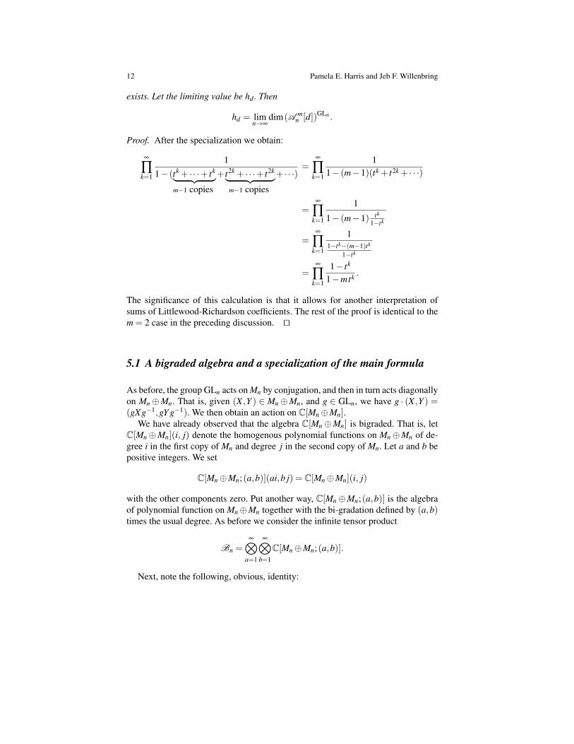
exists. Let the limiting value be hd . Then

hd = limn→∞

dim(A mn [d])GLn .

Proof. After the specialization we obtain:

∞

∏k=1

11− (tk + · · ·+ tk︸ ︷︷ ︸

m−1 copies

+ t2k + · · ·+ t2k︸ ︷︷ ︸m−1 copies

+ · · ·)=

∞

∏k=1

11− (m−1)(tk + t2k + · · ·)

=∞

∏k=1

1

1− (m−1) tk

1−tk

=∞

∏k=1

11−tk−(m−1)tk

1−tk

=∞

∏k=1

1− tk

1−mtk .

The significance of this calculation is that it allows for another interpretation ofsums of Littlewood-Richardson coefficients. The rest of the proof is identical to them = 2 case in the preceding discussion. ut

5.1 A bigraded algebra and a specialization of the main formula

As before, the group GLn acts on Mn by conjugation, and then in turn acts diagonallyon Mn⊕Mn. That is, given (X ,Y ) ∈ Mn⊕Mn, and g ∈ GLn, we have g · (X ,Y ) =(gXg−1,gY g−1). We then obtain an action on C[Mn⊕Mn].

We have already observed that the algebra C[Mn⊕Mn] is bigraded. That is, letC[Mn⊕Mn](i, j) denote the homogenous polynomial functions on Mn⊕Mn of de-gree i in the first copy of Mn and degree j in the second copy of Mn. Let a and b bepositive integers. We set

C[Mn⊕Mn;(a,b)](ai,b j) = C[Mn⊕Mn](i, j)

with the other components zero. Put another way, C[Mn⊕Mn;(a,b)] is the algebraof polynomial function on Mn⊕Mn together with the bi-gradation defined by (a,b)times the usual degree. As before we consider the infinite tensor product

Bn =∞⊗

a=1

∞⊗b=1

C[Mn⊕Mn;(a,b)].

Next, note the following, obvious, identity:

Summing Squares 13

∞

∏k=1

1

1− xkyk

(1−xk)(1−yk)

=∞

∏k=1

(1− xk)(1− yk)

1− (xk + yk).

We observe that this is a specialization of the product in the main formula. Specifi-cally, let qit j = zs where zs is given as the (i, j) entry in the following table.

qit j q q2 q3 q5 q6 · · ·t z1 z2 z4 z7 z11 · · ·t2 z3 z5 z8 z12 z17 · · ·t3 z6 z9 z13 z18 z24 · · ·t4 z10 z14 z19 z25 z32 · · ·t5 z15 z20 z26 z33 z41 · · ·...

......

......

.... . .

Then,

∞

∏k=1

11− (zk

1 + zk2 + zk

3 + · · ·)= ∏

∞k=1

1

1− ∑i, j≥1

(qit j)k

= ∏∞k=1

1

1− qktk

(1−qk)(1−tk)

= ∏∞k=1

(1−qk)(1−tk)

1−(qk+tk).

In this way, the GLn-invariants in the harmonic polynomials on Mn⊕Mn may berelated to the multigraded algebra structure B, as in the singly graded case.

Interestingly, this identity becomes significantly more complicated when gener-alized to harmonic polynomials on more than two copies of the matrices. This willbe the subject of future work.

6 Some combinatorics related to finite fields

In this section, we collect remarks of a combinatorial nature that provide a moreconcrete understanding of the sum of squares that we consider in this paper.

From elementary combinatorics one knows that the infinite product

∞

∏k=1

11−q tk =

∞

∑n=0

∞

∑`=0

pn,`q`tn

where pn,` is the number of partitions of n with exactly ` parts. When q is specializedto a positive integer the coefficients of this series in t has many interpretations.

14 Pamela E. Harris and Jeb F. Willenbring

6.1 The symmetric group

Fix a positive integer d, and a tuple of positive integers d = (d1,d2, · · · ,dm) withd1 + · · ·+dm = d. As before, let Sd denote the subgroup of Sd isomorphic to Sd1 ×·· · × Sdm embedded by letting the ith factor permute the set Ji where {J1, · · · ,Jm}is the partition of {1, · · · ,d} into the m contiguous intervals with |Ji| = di. That is,J1 = {1,2, · · · ,d1}, J2 = {d1 +1, · · · ,d1 +d2}, etc.

The group Sd acts on Sd by conjugation. Let the set of orbits be denoted by O(d).We have

Proposition 3. For any d = (d1, · · · ,dm),

|O(d)|= ∑λ`m

∑µ=(µ(1),···,µ(m))

(cλ

µ

)2

where the inner sum is over all tuples of partitions with µ( j) ` d j.

Proof. We begin with the Peter-Weyl type decomposition of C[Sd ]

C[Sd ]∼=⊕λ`d

(V λ

d

)∗⊗V λ

d .

We then recall that the Littlewood-Richardson coefficients describe the branchingrule from Sd to Sd:

V λ =⊕

µ

cλµV µ(1) ⊗·· ·⊗V µ(m)

.

Combining the above decompositions, we obtain the result from Schur’s Lemma.ut

It is an elementary fact that the Sd-conjugacy class of a permutation σ in Sdis determined by the lengths of the disjoint cycles of σ . A slightly more generalstatement is that the Sd-conjugacy class of σ ∈ Sd is determined by a union of cyclesin which each element of a cycle is “colored” by colors corresponding to J1, · · · ,Jm.It is not difficult to write down a proof of this fact, but we omit it here for spaceconsiderations.

If one fixes d, then the sum over all d-compositions, ∑d |O(d)|, may be inter-preted as the number of d-bead unions of necklaces with each bead colored by mcolors. For example if m = 2, and d = 4, the resulting set may be depicted as:

Summing Squares 15

A single k-bead necklace has Z/kZ-symmetry. If the beads of this necklace arecolored with m colors then the resulting colored necklace may have smaller groupof symmetries. Using Polya enumeration (ie. “Burnsides Lemma”), one can countsuch necklaces by the formula

Nk(m) =1k ∑

r|kφ(r)m

kr .

where φ denotes the Euler totient function6. The theory forming the underpinningsof the above formula may be put in a larger context of cycle index polynomials. Werefer the reader to Doron Zeilberger’s survey article (IV.18 of [GBGL08]).

The generating function for disjoint unions of such necklaces can be given by theproduct

6 That is, φ(r) is the number of positive integers relatively prime to r.

16 Pamela E. Harris and Jeb F. Willenbring

ηm(t) =∞

∏k=1

(1

1− tk

)Nk(m)

That is to say that the number of d-bead necklaces, counted up to cyclic symmetry,is equal to the coefficient of td in η(t). The main formula specializes to

ηm(t) = ∑λ ,µ`d

(cλ

µ

)2t |λ |, (2)

where the sum is over partitions λ and m-tuples of partitions, µ = (µ(1), · · · ,µ(m)).Equation 2 begs for an (explicit) bijective proof which is no doubt obtained by

merging both the Littlewood-Richardson rule and the Robinson-Schensted-Knuthbijection. It is likely that more than one “natural” bijection exists.

6.2 The general linear group over a finite field

Let p denote a prime number, and v ∈ Z+. Set q = pv. Let GLm(q) denote thegeneral linear group of invertible m×m matrices over the field with q elements.The set, Cm(q), of conjugacy classes of GLm(q) has a cardinality of note in that theinfinite products has the following expansion:

∞

∏k=1

1− tk

1−qtk = ∑m=0|Cm(q)|tm,

see [BFH86], and the references within.Note that from Equation 2 we obtain a new formula for the number of conjugacy

classes of GLm(q). Namely,(∞

∏k=1

(1− tk)

)ηq(t) =

∞

∏k=1

(1

1− tk

)Nk(q)−1

.

7 Proof of the main formula

Before proceeding, we require some more notation. Given a partition λ = (λ1 ≥λ2 ≥ ·· ·) with v1 ones, and v2 twos, etc., we will call the sequence (v1,v2, · · ·) thetype vector of λ . Note that `(λ ) = ∑vi, while the size of λ is m = |λ |= ∑λi = ∑ ivi.As is standard, we set

zλ = (v1!1v1)(v2!2v2)(v3!3v3) · · ·

Summing Squares 17

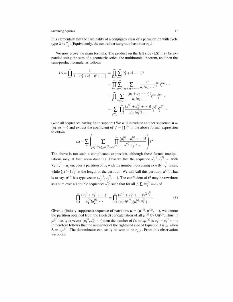
It is elementary that the cardinality of a conjugacy class of a permutation with cycletype λ is m!

zλ. (Equivalently, the centralizer subgroup has order zλ .)

We now prove the main formula. The product on the left side (LS) may be ex-panded using the sum of a geometric series, the multinomial theorem, and then thesum-product formula, as follows

LS =∞

∏k=1

11− (tk

1 + tk2 + tk

3 + · · ·)=

∞

∏k=1

∞

∑u=0

(tk1 + tk

2 + · · ·)u

=∞

∏k=1

∞

∑u=0

∑u1+u2+···=u

u!u1!u2! · · ·

tku11 tku2

2 · · ·

=∞

∏k=1

∑u1,u2,···

(u1 +u2 + · · ·)!u1!u2! · · ·

tku11 tku2

2 · · ·

= ∑u(i)j ,···

∞

∏i=1

(u(i)1 +u(i)2 + · · ·)!u(i)1 !u(i)2 ! · · ·

tiu(i)11 t

iu(i)22 · · ·

(with all sequences having finite support.) We will introduce another sequence, a =(a1,a2, · · ·) and extract the coefficient of ta = ∏ tai

i in the above formal expressionto obtain

LS = ∑a

∑u(i)j :∀ j,∑i iu(i)j =a j

∞

∏i=1

(u(i)1 +u(i)2 + · · ·)!u(i)1 !u(i)2 ! · · ·

ta

The above is not such a complicated expression, although these formal manipu-lations may, at first, seem daunting. Observe that the sequence u(1)j ,u(2)j , · · · with

∑i iu(i)j = a j encodes a partition of a j with the number i occurring exactly u(i)j times,

while ∑ i≥ 1u(i)j is the length of the partition. We will call this partition µ( j). That

is to say, µ( j) has type vector (u(1)j ,u(2)j , · · ·). The coefficient of ta may be rewritten

as a sum over all double sequences u(i)j such that for all j, ∑i iu(i)j = a j of

∞

∏i=1

(u(i)1 +u(i)2 + · · ·)!u(i)1 !u(i)2 ! · · ·

=∞

∏i=1

(u(i)1 +u(i)2 + · · ·)!i∑u(i)j

(u(i)1 !iu(i)1 )(u(i)2 !iu

(i)2 ) · · ·

. (3)

Given a (finitely supported) sequence of partitions µ = (µ(1),µ(2), · · ·), we denotethe partition obtained from the (sorted) concatenation of all µ( j) by ∪µ( j). Thus, ifµ( j) has type vector (u(i)1 ,u(i)2 , · · ·) then the number of i’s in ∪µ( j) is u(i)1 +u(i)2 + · · ·.It therefore follows that the numerator of the righthand side of Equation 3 is zλ whenλ = ∪µ( j). The denominator can easily be seen to be z

µ( j) . From this observationwe obtain

18 Pamela E. Harris and Jeb F. Willenbring

LS = ∑µ

z∪∞j=1µ( j)

∏∞j=1 z

µ( j)z|µ

(1)|1 z|µ

(2)|2 z|µ

(3)|3 · · · .

An application of the Hall scalar product

Let Λn denote the Sn-invariant polynomials (over C as usual) in the indeterminatesx1, · · · ,xn, let Λ [x] = lim←Λn denote the inverse limit. Thus, Λ [x] is the algebra ofsymmetric functions. For a non-negative integer partition λ , we let sλ (x) denote theSchur function. That is, for each n, sλ (x) projects to the polynomial sλ (x1, · · · ,xn)which, as a function on the diagonal matrices, coincides with the character of theGLn-irrep Fλ

n . The set {sλ (x) : λ ` d} is a C-vector space basis of the homogeneousdegree d symmetric functions. We will define a non-degenerate symmetric bilinearform 〈·, ·〉 by declaring

⟨sα(x),sβ (x)

⟩= δαβ for all non-negative integer partitions

α , β . This form is the Hall scalar product.Given an integer m, define pm(x) = xm

1 + xm2 + · · · to denote the power sum sym-

metric function. Given ν ` N, set pν(x) = ∏ pν j(x). We remark that the left side ofthe main formula is easily seen to be ∑ν pν(t).

It is a consequence of Schur-Weyl duality that the coefficients of the Schur func-tion expansion

pν(x) = ∑λ

χλ (ν)sλ (x)

are the characters of the SN-irrep indexed by λ evaluated at any permutation withcycle type ν . It is a standard exercise to see, from the orthogonality of the charactertable, that pν(x) are an orthogonal basis of Λ [x], and 〈pν(x), pν(x)〉= zν .

We next consider another set of indeterminates, y = y1,y2, · · ·. Set Λ [x,y] =Λ [x]⊗Λ [y]. The Hall scalar product extends to Λ [x,y] in the standard way as⟨

f (x)⊗g(y), f ′(x)g′(y)⟩=⟨

f (x), f ′(x)⟩⟨

g(y),g′(y)⟩.

where f (x), f ′(x) ∈Λ [x] and g(y),g′(y) ∈Λ [y]. (We then extend by linearity to allof Λ [x,y].)

The character theoretic consequence of (GLn,GLk)-Howe duality is the Cauchyidentity:

∞

∏i, j=1

11− xiy j

= ∑λ

sλ (x)sλ (y) (4)

(in the infinite sets of variables). In fact, for any pair of dual bases, aλ ,bλ , withrespect to the Hall scalar product, one has ∏

∞i, j=1

11−xiy j

= ∑λ aλ (x)bλ (y). From thisfact one obtains

∞

∏i, j=1

11− xiy j

= ∑λ

pλ (x)pλ (y)/zλ . (5)

From our point of view, we will expand the following scalar product

Summing Squares 19⟨∞

∏k=1

∞

∏i, j=1

11− xiy jtk

,∞

∏i, j=1

11− xiy j

⟩(6)

in two different ways, corresponding to Equations 4 and 5.First by homogeneity of the Schur function and Cauchy’s identity

∞

∏k=1

∑µ

sµ(x)sµ(y)t|µ|k = ∑

µ=(µ(1),µ(2),···)∏

js

µ( j)(x)∏j

sµ( j)(y)t |µ

(1)|1 t |µ

(2)|2 · · · .

Since the multiplication of characters is the character of the tensor product of thecorresponding representations, we have sα sβ = ∑cγ

αβsγ in the x (resp. y) variables.

Expanding the above product gives⟨∞

∏k=1

∞

∏i, j=1

11− xiy jtk

,∞

∏i, j=1

11− xiy j

⟩= ∑

µ

(cλ

µ

)2t |µ

(1)|1 t |µ

(2)|2 · · · .

Secondly, the scalar product in (6) may be expressed as⟨∞

∏k=1

∑µ(k)

pµ(k)(x)p

µ(k)(y)/zµ(k) t |µ

(k)|,∑λ

pλ (x)pλ (y)/zλ

⟩.

We observe that ∏∞k=1 p

µ(k) = pλ where λ = ∪∞k=1µ(k).

7.1 A remark from “Macdonald’s book”

The results presented in this paper emphasize describing the cardinality of an or-bit space by a sum of Littlewood-Richardson coefficients. It is important to note,however, that the main formula can be written simply as

∑ν

pν(x) = ∑µ

(∑λ

(cλ

µ

)2)

xµ(1)

1 xµ(2)

2 xµ(3)

1 · · ·

So from the point of view of [Mac95], one realizes that the main formula is sim-ply a way of expanding ∑ pν(x). With remark in mind, we recall the “standard”viewpoint.

For a non-negative integer partition δ = (δ1 ≥ δ2 ≥ ·· ·) let xδ = xδ11 xδ2

2 xδ33 · · ·.

The monomial symmetric function, mδ (x), is the sum over the orbit obtained by allpermutations of the variables. The monomial symmetric functions are a basis for thealgebra Λ .

zThe question becomes obtaining an expansion of ∑γ pγ(x) into monomial sym-metric functions. This question is answered immediately by observing the expansionof pγ into monomial symmetric functions, which can be found in [Mac95] on page

20 Pamela E. Harris and Jeb F. Willenbring

102 of Chapter I, Section 6. For partitions γ and δ define L(γ,δ ) by the expansion

pγ(x) = ∑δ

Lγδ mδ (x).

We next provide a combinatorial description of Lγδ . Let γ denote a partition oflength `. Given an integer valued function, f , defined on {1,2,3, · · · , `}, set

f (γ)i = ∑j: f ( j)=i

ν j

for each i≥ 1.The sequence ( f (γ)1, f (γ)2, f (γ)3, · · ·) does not have to be weakly decreasing.

For example, if γ = (1,1,1) and f (1) = 1, f (2) = 4 and f (3) = 4 then f (γ)1 = 1,f (γ)4 = 2 and f (γ)k = 0 for all k 6= 1,4. However, often this sequences does definea partition. We have

Proposition 4. Lγ,δ is equal to the number of functions f such that f (γ) = δ .

Proof. See [Mac95] Proposition I (6.9) ut

From Proposition 4 and the main formula, we obtain

Corollary 1. Given a partition δ , the cardinality of

{ f | for some parition γ , f (γ) = δ }

is equal to

∑λ

∑µ

(cλ

µ

)2

where the sum is over all µ such that |µ( j)|= δ j for all j and |λ |= |µ|.

References

[BFH86] David Benson, Walter Feit, and Roger Howe, Finite linear groups, the Commodore64, Euler and Sylvester, Amer. Math. Monthly 93 (1986), no. 9, 717–719, DOI10.2307/2322289. MR863974 (87m:05011) ↑16

[Che55] C. Chevalley, Sur certains groupes simples, Tohoku Math. J. (2) 7 (1955), 14–66(French). MR0073602 (17,457c) ↑3

[Ful97] William Fulton, Young tableaux, London Mathematical Society Student Texts, vol. 35,Cambridge University Press, Cambridge, 1997. With applications to representationtheory and geometry. MR1464693 (99f:05119) ↑1

[GW09] Roe Goodman and Nolan R. Wallach, Symmetry, representations, and invariants,Graduate Texts in Mathematics, vol. 255, Springer, Dordrecht, 2009. MR2522486↑1, 6

[GBGL08] Timothy Gowers, June Barrow-Green, and Imre Leader (eds.), The Princeton com-panion to mathematics, Princeton University Press, Princeton, NJ, 2008. MR2467561(2009i:00002) ↑15

[Har11] Pamela E. Harris, On the adjoint representation of sln and the Fibonaccinumbers, C. R. Math. Acad. Sci. Paris 349 (2011), no. 17-18, 935–937,DOI 10.1016/j.crma.2011.08.017 (English, with English and French summaries).MR2838238 ↑4

[Hes80] Wim H. Hesselink, Characters of the nullcone, Math. Ann. 252 (1980), no. 3, 179–182, DOI 10.1007/BF01420081. MR593631 (82c:17004) ↑4

[Kos63] Bertram Kostant, Lie group representations on polynomial rings, Amer. J. Math. 85(1963), 327–404. MR0158024 (28 #1252) ↑3, 10

[Mac95] I. G. Macdonald, Symmetric functions and Hall polynomials, 2nd ed., Oxford Mathe-matical Monographs, The Clarendon Press Oxford University Press, New York, 1995.With contributions by A. Zelevinsky; Oxford Science Publications. MR1354144(96h:05207) ↑1, 19, 20

[Pro76a] Claudio Procesi, The invariants of n×n matrices, Bull. Amer. Math. Soc. 82 (1976),no. 6, 891–892. MR0419490 (54 #7511) ↑7

[Pro76b] C. Procesi, The invariant theory of n×n matrices, Advances in Math. 19 (1976), no. 3,306–381. MR0419491 (54 #7512) ↑7

[WW00] N. R. Wallach and J. Willenbring, On some q-analogs of a theorem of Kostant-Rallis, Canad. J. Math. 52 (2000), no. 2, 438–448, DOI 10.4153/CJM-2000-020-0.MR1755786 (2001j:22020) ↑4

[Wil07] Jeb F. Willenbring, Stable Hilbert series of S(g)K for classical groups, J. Alge-bra 314 (2007), no. 2, 844–871, DOI 10.1016/j.jalgebra.2007.04.014. MR2344587(2008j:22021) ↑3

21