NBER WORKING PAPER SERIES

RATIONAL CAPITAL BUDGETINGIN AN IRRATIONAL WORLD

Jeremy C. Stein

Working Paper 5496

NATIONAL BUREAU OF ECONOMIC RESEARCH1050 Massachusetts Avenue

Cambridge, MA 02138March 1996

This research is supported by the National Science Foundation, and the International FinancialServices Research Center at MIT. Thanks to Maureen O'Donnell for assistance in preparing themanuscript, and to Michael Barclay, Doug Diamond, Steve Kaplan, Jay Ritter, Dick Thaler, LuigiZingales, an anonymous referee, and seminar participants at the NBER for helpful comments andsuggestions. This paper is part of NBER's research programs in Asset Pricing and CorporateFinance. Any opinions expressed are those of the author and not those of the National Bureauof Economic Research.

© 1996 by Jeremy C. Stein. All rights reserved. Short sections of text, not to exceed twoparagraphs, may be quoted without explicit permission provided that full credit, including ©notice, is given to the source.

NBER Working Paper 5496March 1996

RATIONAL CAPITAL BUDGETINGIN AN IRRATIONAL WORLD

ABSTRACT

This paper addresses the following basic capital budgeting question: Suppose that cross-

sectional differences in stock returns can be predicted based on variables other than beta (e.g.,

book-to-market), and that this predictability reflects market irrationality rather than compensation

for fundamental risk. In this setting, how should companies determine hurdle rates? I show how

factors such as managerial tune horizons and financial constraints affect the optimal hurdle rate.

Under some circumstances, beta can be useful as a capital budgeting tool, even if it is of no use

in predicting stock returns.

Jeremy C. SteinE52-448, Sloan School of ManagementMassachusetts Institute of Technology50 Memorial DriveCambridge, MA 02142-1347and NBER

I. Introduction

The last several years have not been good ones for the capital asset pricing model

(CAPM). A large volume of recent empirical research has found that: i) cross-sectional stock

returns bear little or no discernible relationship to beta; and ii) a number of other variables

besides beta have substantial predictive power for stock returns. For example, one variable that

has been shown to be an important and reliable predictor is the book-to-market ratio: the higher

a firm's book-to-market, the greater its conditional expected return, all else equal)

In light of these empirical results, this paper addresses a simple, yet fundamental

question: What should the academic finance profession be telling MBA students and

practitioners about how to set hurdle rates for capital budgeting decisions? Can we still follow

the standard textbook treatments with a clear conscience and a straight face, and march through

the mechanics of how to do weighted-average-cost-of-capita] or adjusted-present-value

calculations based on the CAPM? Or should we abandon the CAPM for capital budgeting

purposes in favor of alternative models that seem to do a better job of fitting actual stock return

data?

If one believes that the stock market is efficient, and that the predictable excess returns

documented in recent studies are therefore just compensation for risk--risk that is for some

'Early work on the predictive power of variables other than beta includes Banz (1981), Basu(1983) Bhandai-j (1988), DeBondt and Thaler (1985), Jaffe, Keim and Westerfield (1989), Keim(1983), Rosenberg, Reid and Lanstein (1985), and Stattman (1980). See Fama (1991) for adetailed survey of this literature. More recent papers that have focused specifically on book-to-market as a predictive variable include Chan, Hamao, and Lakonishok (1991) Fama and French(1992), Lakonishók, Shleifer and Vishny (1994), Davis (1994), and Chan, Jegadeesh andLakonishok (1995).

1

reason not well-captured by beta--then the answer to the question is simple. According to

standard finance logic, in an efficient market the hurdle rate for an investment in any given asset

should correspond exactly to the prevailing expected return on the stock of a company that is

a pure-play in that asset. The only operational question is which regression specification gives

the best estimates of expected return. Thus the inevitable conclusion is that one must throw out

the CAPM and in its place use the "new and improved" statistical model to set hurdle rates. For

shorthand, I will label this approach to setting hurdle rates the NEER approach, for New

Estimator of Expected Return.

As an example of the NEER approach, consider a chemical company that currently has

a low book-to market ratio, and hence--according to an agreed-upon regression specification--a

low expected return. If the company were considering investing in another chemical plant, this

approach would argue for a relatively low hurdle rate. The implicit economic argument is this:

the low book-to-market ratio is indicative of the low risk of chemical-industry assets. Given this

low risk, it makes sense to set a low hurdle rate. Of course, if the chemical company's book-to-

market ratio--and hence its expected return—were to rise over time, then the hurdle rate for

capital budgeting purposes would have to be adjusted upward.

This NEER approach to capital budgeting is advocated by Fama and French (1993).

Fama and French couch the predictive content of the book-to-market ratio and other variables

in a linear multifactor-mcyjel setting that they argue can be interpreted as a variant of the

arbitrage pricing theory (APT) or intertemporal capital asset pricing model (ICAPM). They then

conclude: "In principle, our results can be used inany application that requires estimates of

expected stock returns. The list includes...estimating the cost of capital." (p. 53)

2

However, it is critical to the Fama-French logic that the return differentials associated

with the book-to-market ratio and other predictive variables be thought of as compensation for

fundamental risk. While there seems to be fairly widespread agreement that variables such as

book-to-market do indeed have predictive content, it is much less clear that this reflects anything

having to do with risk. Indeed, several recent papers find that there is very little affirmative

evidence that stocks with high book-to-market ratios are riskier in any measurable sense.2

An alternative interpretation of the recent empirical literature is that investors make

systematic errors in forming expectations, so that stocks can become significantly over- or

undervalued at particular points in time. As these valuation errors correct themselves, stock

returns will move in a partially predictable fashion. For example, a stock that is overvalued

relative to fundamentals will tend to have a low book-to-market ratio. Over time, this

overvaluation will work its way out of the stock price, so the low book-to-market ratio will

predict relatively low future returns.3

In a world where predictable variations in returns are driven by investors' expectationai

errors, it is no longer obvious that one should set hurdle rates using a NEER approach. The

strong classical argument for such an approach rests in part on the assumption that there is a

one-to-one link between the expected return on a stock and the fundamental economic risk of

the underlying assets. If this assumption is not valid, the problem becomes more complicated.

2See, e.g., Lakonishok, Shleifer and Vishny (1994), MacKinlay (1995), and Daniel andTitman (1995). The latter paper takes direct issue with the Fama-French (1993) notion that thebook-to-market effect can be given a multifactor risk interpretation.

3For evidence supporting this interpretation, see Lakonishok, Shleifer and Vishny (1994),and LaPorta et al (1995).

3

Think back to the example of the chemical company with the low book-to-market ratio. If the

low value of the ratio--and hence the low expected return—is not indicative of risk, but rather

reflects the fact that investors are currently overoptimistic about chemical industry assets, does

it make sense for rational managers to set a low hurdle rate and invest aggressively in acquiring

more such assets?

The key point is that when the market is inefficient, there can be a meaningful distinction

between a NEER approach to hurdle rates, and one that focuses on a measure of Fundamental

Asset Risk--which I will call a FAR approach. A FAR approach involves looking directly at

the variance and covariance properties of the cashflows on the assets in question. In the

chemical company case, this might mean assigning a high hurdle rate if, e.g., the cashflows

from the new plant were highly correlated with the cashflows on other assets in theeconomy—

irrespective of the company's current book-to-market ratio or the conditional expected return on

its stock.

Given this distinction between the NEER and FAR approaches, the main goal of this

paper is to assess the relative merits of the two, and to illustrate how one or the other may be

preferred in a given set of circumstances. To preview the results, I find that, loosely speaking,

a NEER approach makes the most sense when either: i) managers are interested in maximizing

short-term stock prices; or ii) the firm faces financial constraints (in a sense which I will make

precise.) In contrast, a FAR approach is preferable when managers are interested in maximizing

long-run value, and the firm is not financially constrained.

The fact that a FAR approach can make sense in some circumstances leads to an

interesting and somewhat counterintujtive conclusion: in spite of its failure as an empirical

4

description of actual stock returns, the CAPM (or something quite like it) may still be quite

useful from a prescriptive point of view in capital budgeting decisions. This is because beta--if

calculated properly--may continue to be a reasonable measure of the fundamental economic risk

of an asset, even if it has little or no predictive power for stock returns. However, it must be

emphasized that this sort of rationale for using the CAPM does not apply in all circumstances.

As noted above, when managers have short horizons or when the firm faces financial constraints,

the CAPM--or any FAR-based approach--will be inappropriate to the extent that it does not

present an accurate picture of the expected returns on stocks.

Before proceeding, I should also reiterate that the entire analysis which follows is based

on the premise that the stock market is inefficient. More precisely, cross-sectional differences

in expected returns will be assumed throughout to be driven in part by expectational errors on

the part of investors. I make this assumption for two reasons. First, it strikes me that at the

least, there is enough evidence on the table at this point for one to question market efficiency

seriously and wonder what capital budgeting rules would look like in its absence. Second, as

discussed above, the efficient-markets case is already well-understood and there is little to add.

In any event, however, readers can judge for themselves whether or not they think the

inefficient-markets premise is palatable as a basis for thinking about capital budgeting.

Of course, this is not the first paper to raise the general question of whether and how

stock market inefficiencies color investment decisions. This question dates back at least to

Keynes (1936), who raises the possibility that "certain classes of investment are governed by the

average expectation of those who deal on the Stock Exchange as revealed in the price of shares,

5

rather than by the genuine expectations of the professional entrepreneur. " (page 151) More

recent contributions include Bosworth (1975), Fischer and Merton (1984), DeLong et al (1989),

Morck, Shleifer and Vishny (1990) and Blanchard, R]ee and Summers (1993). The latter two

pieces are particularly noteworthy in that they stress--as does this one--the importance of

managers' time horizons and financing constraints. The contribution of this paper relative to

these earlier works is twofold: first, it provides a simple analytical framework in which the

effects of horizons and financing constraints can be seen clearly and explicitly; and second, it

focuses on the question of what are appropriate risk-adjusted hurdle rates, thereby developing

an inefficient-markets analog to textbook treatments of capital budgeting under uncertainty.5

The remainder of the paper is organized as follows. In Section II, I examine the link

between managers' time horizons and hurdle rates, leaving aside for simplicity the issue of

financial constraints. This section establishes that a FAR approach is more desirable when the

time horizon is longer. In Section III, I introduce the possibility of financial constraints, and

show how these have an effect similar to shortening the time horizon--i.e., financial constraints

tend to favor a NEER approach. In Section IV, I take up measurement issues. Specifically, if

one decides to use a FAR approach, what is the best way to get an empirical handle on

fundamental asset risk? To what extent can one rationalize the use of beta--as conventionally

calculated--as an attempt to implement a FAR approach? Section V briefly discusses a number

of extensions and variations of the basic framework, and Section VI fleshes out its empirical

4As will become clear, in terms of the language of this paper Keynes is effectivelyexpressing the concern that managers will adopt a NEER approach to capital budgeting.

51n contrast, the informal discussion in Blanchard, Rhee and Summers (1993) assumes riskneutrality, and hence does not speak to the whole issue of risk-adjusted hurdle rates.

6

implications. Section VII concludes.

II. Time Horizons and Optimal Hurdle Rates

I consider a simple two-period capital budgeting model that is fairly standard in most

respects. At time 0, the firm in question is initially all equity financed. It already has physical

assets in place that will produce a single net cashflow of F at time 1. From theperspective of

time 0, F is a random variable that is normally distributed. The firm also has the opportunity

to invest $1 more at time 0 in identical assets--i.e., if it chooses to invest, itsphysical assets will

yield a total of 2F at time I. The decision of whether or not to invest is the only one facing the

firm at time 0. If it does invest, the investment will be financed with riskiess debt that is fairly

priced in the marketplace. There is no possibility of issuing or repurchasing shares. (As will

become clear in Section III, allowing the firm to transact in theequity market at time 0 may in

some circumstances alter the results.) There are also no taxes.

The manager of the firm is assumed to have rational expectations. I denote the

manager's rational time-0 forecast of F by F EF. The firm's other outside shareholders,

however, have biased expectations. Their biased forecast of F is given by P EF(l +5).

Thus S is a measure of the extent to which outside investors are overoptimistic about the

prospects for the firm's physical assets. This bias in assessing the value of physical assets is the

only way in which the model departs from the standard framework. Outside investorsare

perfectly rational in all other respects. For example, they perceive all variances and covariances

accurately. Thus the degree of irrationality that is being ascribed to outside investors is in a

sense quite mild. It would certainly be interesting to entertain alternative models of such

7

irrationality, but in the absence of clear-cut theoretical guidance, the simple form considered

here seems like a natural place to start.

The shares in the firm are part of a larger market portfolio. The net cashflow payoff on

the market portfolio at time 1 is given by M, which is also normally distributed. For simplicity,

I assume that both the manager of the firm and all outside investors have rational expectations

about M. Thus I am effectively assuming that investors make firm-level mistakes in assessing

cashflows, but that these mistakes wash out across the market as a whole.' I denote the price

of the market portfolio at time 0 by M, and define RM M/PM - I as the realized percentage

return on the market.

The final assumption is that the price of the firm's shares is determined solely by the

expectations of the outside investors. This amounts to saying that even though the manager may

have a different opinion, he is unable or unwilling to trade in sufficient quantity to affect the

market price.

With the assumptions in place, the first thing to do is to calculate the initial market price

P of the firm's shares, before the investment decision has been made at time 0. This is an easy

task. Note that we are operating in a standard mean-variance framework, with the only

exception being that investors have biased expectations. This bias does not vitiate many of the

classical results that obtain in such a framework. First of all, investors will all hold the market

portfolio, and the market portfolio will be--in their eyes--mean-variance efficient. Second, the

equilibrium return required by investors in firm's equity, k, will be given by:

'Or said somewhat more mildly, the manager of the firm does not disagree with outsideinvestors' assessment of M.

8

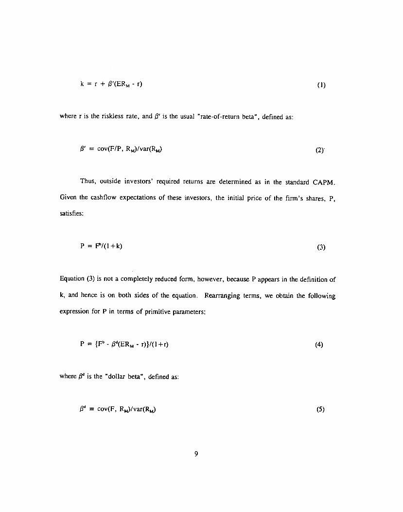
k=r+13'(ERM-r) (1)

where r is the riskless rate, and I3' is the usual "rate-of-return beta", defined as:

/3' cov(F/P, RM)/var(R) (2)

Thus, outside investors' required returns are determined as in the standard CAPM.

Given the cashflow expectations of these investors, the initial price of the firm's shares, P,

satisfies:

P = P/(l+k) (3)

Equation (3) is not a completely reduced form, however, because P appears in the definition of

k, and hence is on both sides of the equation. Rearranging terms, we obtain the following

expression for P in terms of primitive parameters:

P = {F" - 13d(ERM - r)}/(l+r) (4)

where 13d is the "dollar beta", defined as:

cov(F, RM)Ivar(RM) (5)

9

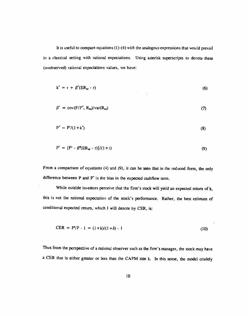
It is useful to compare equations (1 )-(4) with theanaiogous expressions that would prevail

in a classical setting with rational expectations. Using asterisk superscripts to denote these

(unobserved) rational expectations values, we have:

k = r + (ERM - r) (6)

cov(F/P', RM)/var(R,.) (7)

= FrI(l+k) (8)

= {F - (ERM - r)}/(l +r) (9)

From a comparison of equations (4) and (9), it can be seen that in the reduced form, the only

difference between P and P is the bias in the expected cashflow term.

While outside investors perceive that the firm's stock will yield an expected return of k,

this is not the rational expectation of the stock's performance. Rather, the best estimate of

conditional expected return, which I will denote by CER, is:

CER = P/P-i = (1+k)/(l+ô)- 1 (10)

Thus from the perspective of a rational observer such as the firm'smanager, the stock may have

a CER that is either greater or less than the CAPM rate k. In this sense, the model crudely

10

captures the empirical regularity that•there are predictable returns on stocks that are not related

to their betas. These predictable returns simply reflect the biases of the outside investors. Note

that when = 0, so that outside investors have no bias, CER = k = k'. When ó > 0, so that

the stock is overpriced, CER < k < k'. And conversely, when ô < 0, CER > k > k'.

We are now ready to address the question of the optimal hurdle rate. To do so, we have

to be clear about the objective function that is being maximized. There are two distinct

possibilities. First, one might assume that the manager seeks to maximize the stock price that

prevails at time 0, immediately after the investment decision has been made. This is the same

as saying that the manager tries to maximize outside investors' perception of value.

Alternatively, one might posit that the manager seeks to maximize the present value of the firm's

future cashflows, as seen from his more rational Derspective.

In principle, one can think of reasons why managers might tend to favor either objective.

For example, if they are acting on behalf of shareholders (including themselves) who have to

sell their stock in the near future for liquidity reasons, they will be more inclined to maximize

current stock prices. In contrast, if they are acting on behalf of shareholders (including

themselves) who will be holding for the longer term--e.g., due to capital gains taxes or other

frictions--they will be more inclined to maximize the present value of future cashflows. In what

follows, I treat the managerial time horizon as exogenous, although in a fuller model, it would

be endogenously determined.7

7This distinction between maximizing current stock prices versus maximizing management'sperception of long-run value also arises in the literature on investment and financing decisionsunder asymmetric information. See, e.g., Miller and Rock (1985) and Stein (1989) for a fullerdiscussion of the forces that shape the tradeoff between the two objectives. One potentiallyimportant factor has to do with agency considerations. Specifically, shareholders may—in

11

Let us first consider the "short-horizon" case where the goal is to maximize the current

stock price. It is easy to see that in this case, the "value" created by investing is simply

(P - 1). Intuitively, as long as the market's current valuation of the assets in question exceeds

the acquisition cost, the current stock price will be increased if the assets are purchased. To

translate this into a statement about hurdle rates, note that from management's perspective, the

expected cashfiow on the investment is F. Thus the short-horizon hurdle rate, defined as

has the property that the gross discounted value of the investment, P1(1 +hs), equals P. Using

equation (10), it follows immediately that:

Proposition I: In the short-horizon case, the manager should discount his expected

cashflow P at a hurdle rate hs = CER. In other words, the manager should take a NEER

approach and use the conditional expected return on the stock as the hurdle rate.

One way to think about Proposition 1 is that if the manager is interested in maximizing

the current stock price, he must cater to any misperceptions that investors have. Thus if

investors are overly optimistic about the prospects for the firm's assets--thereby leading to a low

value of CER--the manager should be willing to invest very aggressively in these assets, and

hence should adopt a low hurdle rate.

Things work quite differently in the "long-horizon" case where the manager seeks to

maximize his perception of the present value of future cashflows. In thiscase, the "value"

response to agency problems--impose on managers an incentive scheme or corporate policies thathave the effect of making the managers behave as if they were more concerned withmaximizingcurrent stock prices. This issue is discussed in more detail in Section V.C below.

12

created by investment is (P - 1). That is, the manager should only invest if the rational

expectations value of the assets exceeds their acquisition cost. Thus the long-horizon hurdle rate

h'- has the property that P1(1 +hL) = P. Using equation (8), this leads to:

Proposition 2: In the long-horizon case, the manager should discount his expected

cashflow P at a hurdle rate hL = k'. In other words, the manager should take a FAR approach

and choose a hurdle rate that reflects the fundamental risk of the assets in question and that is

independent of outside investors' bias .

Proposition 2 suggests that hurdle rates in the long-horizon case should be set in a

"CAPM-like" fashion. This is very close in spirit to the standard textbook prescription.

However, the one major caveat is that unlike in the textbook world, one needs to be more

careful in the empirical implementation. According to equations (6) and (7), the i1 that is

needed for this CAPM-like calculation is the (unobserved) beta that would prevail in a rational

expectations world, as this is the correct measure of the fundamental risk borne by long-horizon

investors. And given that the underlying premise throughout is that the stock market is

inefficient, one cannot blithely make the usual assumption that a beta calculated in the traditional

way—with a regression of the firm's stock returns on market returns--will provide an adequate

proxy for the j3' that is called for in Proposition 2. Thus there is a non-trivial set of issues

surrounding the best way to measure 9'. These issues are taken up in detail in Section IV

below.

13

III. Financing Considerations and Optimal Hurdle Rates

So far, the analysis has ignored the possibility that the firm might either issue or

repurchase shares. Given the premise--that the market is inefficient and that managers know it--

this is a potentially important omission. First of all, there will naturally be circumstances in

which managers wish to engage is stock issues or repurchases to take advantage of market

inefficiencies. Second, and more significantly for our purposes, there may in some cases be a

link between these opportunistic financing maneuvers and the optimal hurdle rate for capital

budgeting.

The goal of this section is to explore these links between financing considerations and

hurdle rates. I begin with a general formulation of the problem. I then consider a series of

special cases that yield particularly crisp results and that highlight the most important intuition.

A. A general formulation of the problem

When a manager chooses an investment-financing combination in an inefficient market,

there are in general three considerations that must be taken into account: 1) the net present value

of the investment; 2) the "market timing" gains or losses associated with any share issues or

repurchases; and 3) the extent to which the investment-financing combination leads to any costly

deviations from the optimal capital structure for the firm. Thus in order to specify an overall

objective function, one must spell out each of these considerations in detail.

1One possibility that I ignore for the time being is that managers might wish to takeadvantage of market inefficiencies by transacting in the stock of other firms. This considerationis taken up in Section V.D below, and as will be seen, need not materially affect the conclusionsof the analysis.

14

I. The net present value of investment

As will become clear, to the extent that financing considerations have any consequence

at all for hurdle rates, it is to effectively shorten managers' time horizons--i.e., to make them

behave in more of a NEER fashion. Therefore, to make the analysis interesting, I assume that

absent financing concerns, managers take a FAR approach, and seek to maximize the present

value of future cashflows.

For the purposes of doing a bit of calculus, I generalize slightly from the previous

section, and allow the amount invested at time 0 to be a continuous variable K. The gross

expected proceeds at time I from this investment are given by f(K), which is an increasing,

concave function. The relevant FAR-based definition of the net present value of investment is

thus f(K)P'IP - K, or equivalently, f(K)/(1 +V) - K, where k' continues to be given by equations

(6) and (7).

2. Market timing gains or losses

Denote by E the dollar amount of equity raised by selling new shares at time 0. Thus

if E > 0, this should be interpreted as an equity issue by the firm; if E < 0, this should be

interpreted as a repurchase. If the firm is able to transact in its own equity without any pnce

pressure effects, the market timing gains from the perspective of the manager are given simply

by the difference between the market's initial time-0 valuation of the shares and the manager's

time-C) valuation. For a transaction of size E, this market timing gain is simply E(1 -

9As above, I continue to assume that when the firm issues debt, this debt is fairly priced,so that there are no market timing gains or losses. This assumption can be relaxed withoutaffecting the qualitative results that follow.

15

Of course, it is extreme and unrealistic to assume that there are no price-pressureeffects

whatsoever, particularly if the implied equity transactions turn out to be large in absolute

magnitude. At the same time, given the premise of investor irrationality, one does not

necessarily want to go to the other extreme--represented by rational asymmetric information

models such as Myers and Majiuf (1984)--and assume that the announcement effects of a share

issue or repurchase are such that they on average completely eliminate the potential for market

timing gains.

As a compromise, I adopt a simple, relatively unstructured formulation in which the net-

of-pt-ice-pressure market timing gains are given by E(l - P'/P) - i(E). Here i(E) captures the

price-impact-related losses associated with an equity transaction of size E, with i(O) = 0. The

only other restrictions I impose a priori are that: 1) when E > 0, dudE 0, and conversely,

when E < 0, dudE � 0; and 2) d2i/dE2 �0 everywhere. In words, equity issues tend to

knock prices down, while repurchases push prices up, with larger effects for larger transactions

in either direction.

The i(E) function can be interpreted in terms of a couple of different underlying

phenomena. First, it might be that even irrational investors do update their beliefs somewhat

when they see management undertaking an equity transaction. However, in contrast to rational

models based on asymmetric information, the updating is insufficient to wipe out predictable

excess returns. This interpretation fits with the spirit of recent studies that suggest that the

market underreacts dramatically to the information contained in both seasoned equity offerings

16

and repurchases. '° Alternatively, in the case of share repurchases, i(E) might be thought of

as reflecting the premium that tendering investors require to compensate them for capital gains

taxes.

3. The costs of deviating from optimal capital structure

Finally, one must consider the possibility that a given investment-financing combination

will lead to a sub-optimal capital structure. For example, if a firm decides to invest a great

deal, and to engage in repurchases to take advantage of a low stock price, leverage may increase

to the point where expected costs of financial distress become significant. To capture this

possibility in a simple way, I assume that the optimal debt ratio for the firm is given by D, and

that prior to the investment and financing choices at time 0, the firm is exactly at this optimum.

Thus after it has invested an amount K and raised an amount of new equity E, it will be

overleveraged by an amount L K(l-D) - E. I assume that this imposes a cost of Z(L).

Again, I do not put too much a priori structure on the Z(L) function. By definition,

things are normalized so that Z(0) = 0. In principle, straying in either direction from the

optimum of 0 can be costly--too little debt may be a problem as well as too much debt.

Moreover, to the extent that there are costs of straying, these costs are a convex function of the

distance from the optimum. As with the i(E) function, this implies that: 1) dZ/dL � 0 when

L > 0, and conversely, dZJdL � 0 when L < 0; and 2) d2Z/dL2 � 0 everywhere.

'°See, e.g., Loughran and Ritter (1995), Spiess and Affleck-Graves (1995) and Cheng (1995)on seasoned equity offerings, and Ikenberry, Lakonishok and Vermaelen (1995) on sharerepurchases.

17

4. Optimal investment and financing decisions

Taking all three considerations together, the manager's objective function is:

max f(K)P7P - K + E(1 - P/P) - i(E) - Z(L) (11)

subject to: L K(1-D) - E.

The first-order conditions for this problem are:

df/dK - (1 + (1-D)dZ/dL)F/P = 0 (12)

(1 - P'/P) - dudE + dZJdL = 0 (13)

A little algebra shows that optimal investment therefore satisfies:

df/dK = DF/P + (l-D)(F'/P + dudE)

= D(1+k) + (l-D)(1 + CER + dudE) (14)

B. Case-by-case analysis

Since the intuition underlying equation (14) may not be immediately apparent, it is useful

to go through a series of special cases to build an understanding of the various forces at work.

18

1. Capital structure is not a binding constraint

The first, simplest limiting case to consider is one in which dZ/dL 0--i.e., there are

no marginal costs or benefits to changing leverage, other than those that come directly from

issuing or repurchasing shares at time 0. This condition would clearly hold in a world with no

taxes and no costs of financial distress, where, were it not for the mispricing of the firm's stock,

the Modigliani-Miller theorem would apply. But more generally, one need not make such strong

assumptions for this case to be (approximately) relevant. All that is really required is that the

Z function be flat in the neighborhood of the optimal solution. For example, if price-pressure

effects are significant, and diminishing returns to investment set in quickly, the firm will only

choose to make small investment and financing adjustments, and thus will never try to push

capital structure very far from its initial position of L = 0. If in addition, the Z function

happens to be flat in this region near 0, the firm will be left in a position where, e.g.,

incremental increases in leverage would have only a trivial impact on costs of financial distress.

When dZ/dL = 0, equations (12) and (13) tell us that investment and financing decisions

are fully separable. Intuitively, this is because capital structure can at the margin adjust

costlessly to take up the slack between the two. The optimal behavior for the firm in this case

is spelled out in the following proposition:

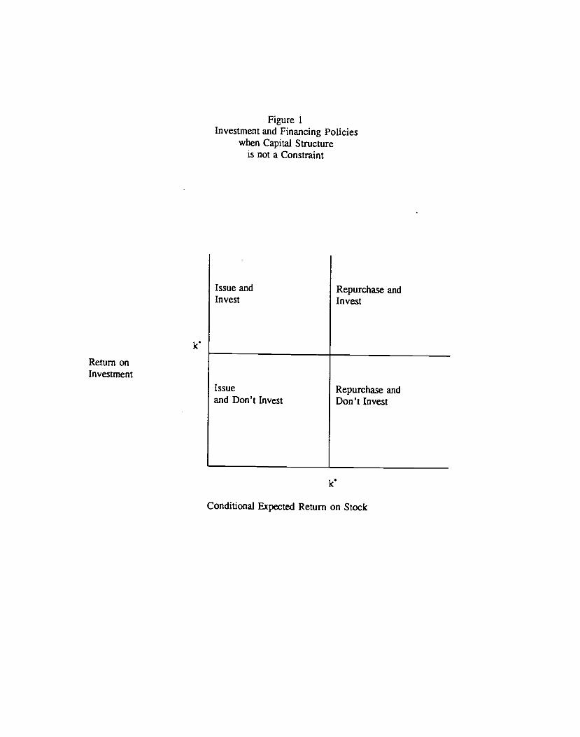
Proposition 3: When capital structure is not a binding constraint, and the manager has

long horizons, the optimal policies are:

--Always set the hurdle rate at the FAR value of k, as in Proposition 2.

--Issue stock if the CER < k; repurchase stock if the CER > k'.

19

Figure 1 illustrates the optimal investment and financing policies. As can be seen, the

two are completely decoupled. When the stock price is low and the CER is high, the firm

repurchases shares. However, because capital structure is fully flexible, the repurchase does not

affect its hurdle rate. Rather, the firm adjusts to the repurchase purely by taking on more debt.

Therefore at the margin, investment should be evaluated vis-a-vis fairly-priced debt finance,

exactly as in Section H above.

Conversely, when the stock price is high and the CER is low, the firm issues shares.

However, it does not have to plow the proceeds of the share issue into investment. These

proceeds can be used to pay down debt or accumulate cash. So there is no reason that the

issuance of 'cheap stocks should lower the hurdle rate for investment.

2. Bindin2 capital structure constraint, no once-pressure effects

The next case to examine is one in which the capital structure constraint is binding, but

where price-pressure effects are absent--i.e., one in which dZ/dL 0 and dudE = 0. In this

case, equation (14) simplifies to:

df/dK = D(l+k') + (l-D)(l + CER) (15)

Based on equation (15), we have:

20

Pronosition 4: When the capital structure constraint is binding, and there are no price-

pressure considerations, the optimal hurdle rate has the following properties:

--The hurdle rate is between the NEER and FAR values of CER and k respectively.

--As D approaches 0, the hurdle rate converges to CER, as in Proposition 1.

--As D approaches 1, the hurdle rate converges to k, as in Proposition 2.

The intuition behind Proposition 4 is very simple. When capital structure imposes a

binding constraint, one cannot in general separate investment and financing decisions. This is

perhaps easiest to see in the case where ô < 0, so that the stock is undervalued and the firm

would like to be repurchasing shares. For each dollar that is devoted to investment, there is less

cash available to engage in such repurchases, holding the capital structure fixed. Indeed, in the

extreme case where D = 0--i.e., where the incremental investment has zero debt capacity--each

dollar of investment leaves one full dollar less available for repurchases. Hence in this case,

the opportunity cost of investment is simply the expected return on the stock, as in the NEER

approach.

Thus in the limiting case where D = 0, financial constraints force managers who would

otherwise take a long-run view into behaving exactly as if they were interested in maximizing

short-term stock prices. This is simply because, in order to leave capital structure undisturbed,

any investment must be fully funded by an immediate stock issue. So all that matters is the

market's current assessment of whether the investment is attractive or not.

In the intermediate cases where 0 < D < I, investment need only be partially funded

by a stock issue. This implies that the hurdle rate moves less than one-for-one with the CER

21

on the stock. At the other extreme, when D = 1 and investment can be entirely debt-financed,

the hurdle rate remains anchored at the FAR value of k, irrespective of the CER on the

stock." Figure 2 illustrates the relationship between the hurdle rate and the CER on the stock,

for different values of D.

3. Binding caoital structure constraint and price-pressure effects

The final case to consider is the most general one where the capital structure constraint

is binding and where there are price-pressure effects. This case is most usefully attacked by

breaking it down into sub-cases:

a) Stock is undervalued: < 0

When & < 0, it is easy to show that L > 0. That is, the firm will choose to be

overlevered relative to the static optimal capital structure of L = 0. However, the sign of E is

ambiguous--the firm may either issue or repurchase shares. This ambiguity in E arises because

there are two competing effects: on the one hand, the fact that 5 < 0 makes a repurchase

attractive from a market timing standpoint. On the other hand, given that the firm is investing,

it needs to raise some new equity if does not wish to see its capital structure get too far out of

line. Depending on which effect dominates, there can either be a net repurchase or a share

issue.

"Of course, one should not take this limiting case too literally, given that I have alsoassumed that the firm can issue fairly priced (i.e., nskless) debt.

22

i) Share repurchase: E < 0. In this case, it is straightforward to verify:

Proposition 5: When the capital structure constraint is binding, there aie price-pressure

considerations, .5 < 0 and E < 0, the optimal hurdle rate has the following properties:

--The hurdle rate is always between the NEER and FAR values.

--The stronger are price-pressure effects--i.e., the larger is dudE in absolute magnitude--

the lower is the hurdle rate, all else equal, and therefore the closer it is to the FAR value of k.

Proposition 5 says that this case represents a well-behaved middle ground between the

two more extreme cases covered in Propositions 3 and 4. When price-pressure effects are

strong, the outcome is closer to that in Proposition 3, where capital structure was not a binding

constraint--the hurdle rate is set more according to a FAR approach. This is because price

pressure leads the firm to limit the scale of its repurchase activity. Consequently, capital

structure is not much distorted, and there is less influence of financial constraints on investment.

Of course, when price-pressure effects are very weak, we converge back to the case described

in Proposition 4.

ii) Equity issue: E > 0. The outcome with an equity issue is a bit more

counterintuitive:

23

Proposition 6: When the capital structure constraint is binding, there are price-pressure

considerations, & < 0 and E > 0, the optimal hurdle rate has the following properties:

--The hurdle rate no longer necessarily lies between the NEER and FAR values. In

particular, it may exceed them both, though it will never be below the lower of the two, namely

the FAR value of k.

--The stronger are price-pressure effects--i.e., the larger is dudE in absolute magnitude--

the higher is the hurdle rate, all else equal.

Thus here is a situation--the first we have encountered so far--where the hurdle rate does

not lie between the NEER and FAR values. However, this result has nothing really to do with

the market irrationality that is the focus of this paper. Rather, it is just a variant on the Myers-

Majluf (1984) argument that when investment requires an equity issue, and such an equity issue

knocks stock prices down, there will typically be underinvestment. Indeed, the effect is seen

most cleanly by assuming that there is no irrationality whatsoever--i.e., that & = 0--so that the

NEER and FAR values coincide. Inspection of equation (14) tell us that optimal investment will

satisfy df/dK = (1 +k') + (l-D)di/dE. In other words, the hurdle rate is a markup over the

NEERJFAR value of k', with the degree of this markup determined by the magnitude of the

price-pressure effect.

b) Stock is overvalued; ô > 0

When & > 0, there is no ambiguity about the sign of E. This is because both market

timing considerations and the need to finance investment now point in the same direction,

24

implying a desire to sell stock. So E > 0. This gives rise to a result very similar to that seen

just above:

Proposition 7: When the capital structure constraint is binding, there are price-pressure

considerations, S > 0 and E > 0, the optimal hurdle rate has the following properties:

--The hurdle rate no longer necessarily lies between the NEER and FAR values. In

particular, it may exceed them both, though it will never be below the lower of the two, namely

the NEER value of CER.

—The stronger are price-pressure effects--i.e., the larger is dudE in absolute magnitude--

the higher is the hurdle rate, all else equal.

C. Conclusions on the effects of financin2 considerations

The analysis of this section has shown that financing considerations shape the optimal

hurdle rate in three distinct ways.

The first factor that matters is the shape of the Z function, which measures the degree

to which deviations in capital structure are costly. When such deviations are inconsequential,

this tends to favor a FAR-based approach to setting hurdle rates. In contrast, when such

deviations are costly, the optimal hurdle rate is pushed in the NEER direction.

The second factor is the debt capacity D of the new investment. This second factor

interacts with the first. In particular, the lower is D, the more pronounced an effect capital

structure constraints have, in terms of driving the hurdle rate towards the NEER value.

The third factor is the extent to which share issues or repurchases have price-pressure

25

consequences. In terms of the NEER-FAR dichotomy, the impact of this third factor is

somewhat more ambiguous than that of the other two. One can make a clear-cut statement only

in the case where the firm engages in a stock repurchase; here price-pressure considerations

unambiguously move the hurdle rate closer to the FAR value of k'. However, when the firm

issues equity, all that one can say for sure is that price pressure exerts an upwards influence on

the hurdle rate; it no longer follows that the hurdle rate is pushed closer to the FAR value.

The overall message of this section is that while one can certainly argue in favor of a

FAR-based approach to capital budgeting, the argument is somewhat more delicate than it might

have appeared in Section II, and does not apply in all circumstances. In order for a FAR-based

approach to make sense, not only must managers have long horizons, but they must be relatively

unconstrained by their current capital structures.

IV. Implementing a FAR-Based Approach: Measuring 8

Part of the appeal of a FAR-based approach to capital budgeting is that it appears to be

very close to the textbook CAPM method. However, as noted in Section II above, the one hitch

is that in order to implement a FAR-based approach, one needs to know j3', which is the value

of beta that would prevail in a rational expectations world; i.e., the fundamental risk of the

assets in question. And given the underlying premise of the paper--that the stock market is

inefficient--one cannot simply assume that a beta calculated using observed stock returns will

yield a good estimate of fi'. Thus the following question arises: as a practical matter, how close

to fl can one expect to get using the standard regression methodology for calculating beta?

26

A. Theoretical considerations

In order to clarify the issues, it is useful begin with a more detailed analytical comparison

of the value of a beta computed from actual stock return data--which I will continue to denote

by I3--versus that of 3'. To do so, I will generalize somewhat from the setting of the previous

sections, by entertaining the possibility that there is mispricing of the market as a whole, as well

as mispricing of individual stocks. In addition, and somewhat trivially, I will allow for more

than one period's worth of stock returns.

Note that in any period t, for any stock i, we can always make the following

decomposition:

R,, R + Na (16)

where R, is the observed return on the stock, R',, is the return that would prevail in a rational

expectations world--i.e., the portion of the observed return due to 'fundamentals"--and N1 is the

portion of the observed return due to 'nois&'. We can also make a similar decomposition for

the observed return on the market as a whole, RMI:

RM R'M, + NM, (17)

Clearly, as a general matter, the beta calculated from observed stock returns, if,

cov(R1, RMI)/var(RMJ will not coincide with = cov(ra, RMJ/var(R..). To get a better

intuitive handle on the sources of the difference between ifand a',, it is helpful to consider a

27

simple case where both R, and N,, are generated by one-factor processes, as follows:

= $RMI + (18)

= O,NM, + (19)

where cov(€, ) = 0) In this formulation, 0, represents the sensitivity of stock i's noise

component to the noise component on the market as a whole--i.e., 0, is a "noise betas for

stock i.

It is now easy to calculate /3r:

= {j3var(R' + 0var(NJ + (13+0j)cov(RM,NM))I

{var(R) + var(N.J + 2cov(RM, N,,J} (20)

From (20), one can see how various parameters influence the relative magnitudes if, and

/3. The most important conclusion for our purposes is that it is not obvious a priori that one

will be systematically larger or smaller than the other. Indeed, in some circumstances, they will

be exactly equal. For example, if var(NM) = 0, so that all noise is firm-specific and washes out

at the aggregate level, then if, = a',. Alternatively, the same result obtains if there is market-

'2Note that the two-period model used in Sections H and III above does not quite conformto this specification. This is because all mispricing is assumed to disappear after the first period,which in turn implies that there are not enough degrees of freedom to also assume thatcov(€,, = 0. However, the simple specification of equations (18) and (19) is merely anexpositional device that allows one to illustrate the important effects more clearly.

28

wide noise, but the noise beta 0, equals I3,. Although these cases are clearly special, they do

illustrate a more general point: a stock may be subject to very large absolute pricing errors---in

the sense of var(N) being very large--and yet one might in principle be able to retrieve quite

reasonable estimates of I3, from stock price data.'3 Whether this is true in practice is then a

purely empirical question.

B. Existing evidence

In order to ascertain whether a beta estimated from stock price data does in fact do a

good job of capturing the sort of fundamental risk envisioned in fi', one needs to develop an

empirical analog of 13. A natural, though somewhat crude approach would be as follows.

Suppose one posits that the rational expectations value of a stock is the present value of the

expected cashflows to equity, discounted at a constant rate. Suppose further that cashflows

follow a random walk, so today's level is a sufficient statistic for future expectations. In this

very simple case, it is easy to show that for any given stock i:

= cov(F/F, M/M)/var(M/M) (21)

where F1 and M are the cashflows accruing to stock i and the market as a whole respectively.

This is a quantity that can be readily estimated, and then compared to the corresponding betas

'3A second implication of (20) is that if the market-wide noise is stationary, one might beable to obtain better estimates of $, by using longer-horizon returns. At sufficiently longhorizons, the variance of RM will dominate the other terms in (20), ultimately leading ff toconverge to fit.

29

estimated from stock prices.

In fact, there is an older literature, beginning with Ball and Brown (1969) and Beaver,

Kettler and Scholes (1970), that undertakes a very similar comparison. In this literature, the

basic hypothesis being tested is whether "accounting betas" for either individual stocks or

portfolios are correlated with betas estimated from stock returns)4 In some of this work--

notably Beaver and Manegold (1975)--accounting betas are defined in a way that is very similar

to equation (21), with the primary exception being that an accounting net income number is

typically used in place of a cashflow.

Subject to this one accounting-related caveat, Beaver and Manegold's results would seem

to indicate that there is indeed a fairly close correspondence between stock market betas and

fundamental risk. For example, with 10-stock portfolios, the Spearman correlation coefficient

between accounting and stock return betas varies from about .70 to .90, depending on the exact

specification used.

The bottom line is that both theoretical considerations and existing empirical evidence

suggest that, at the least, it may not be totally unreasonable to simultaneously assume that:

1) stocks are subject to large pricing errors; and yet 2) a beta estimated from stock returns can

provide a good measure of the fundamental asset risk variable 13 needed to implement a FAR-

"The motivation behind this earlier literature is quite different from that here, however. Inthe l970's work, market efficiency is taken for granted, and the question posed is whetheraccounting measures of risk are informative, in the sense of being related to market-basedmeasures of risk (which are assumed to be objectively correct). In addition to the papersmentioned in the text, see also Gonedes (1973, 1975) for further examples of this line ofresearch.

30

based approach to capital budgeting.'5

V. Extensions and Variations

The analysis in Sections II and Ill above has made a number of strong simplifying

assumptions. In some cases, it is easy to see how the basic framework could be extended so as

to relax these assumptions; in other cases, it is clear that the problem becomes substantially more

complex and that more work is required,

A. Alternative measures of fundamental risk

One assumption that has been maintained to this point is that the underlying structure of

the economy is such that j3 is the appropriate summary statistic for an asset's fundamental risk.

This need not be the case. One can redo the entire analysis in a world where there is a

multifactor representation of fundamental risk, such as that which emerges from the APT or the

ICAPM. In either case, the spirit of the conclusions would be unchanged--these alternative risk

measures would be used instead of $' to determine FAR-based hurdle rates. Whether or not

such FAR-based hurdle rates would actually be used for capital budgeting purposes--as opposed

to NEER-based hurdle rates--would continue to depend on the same factors identified above,

namely managers' time horizons and financing constraints.

'50f course, this statement may be reasonable on average and at the same time be moreappropriate for some categories of stocks than for others. To take just one example, somestocks--e.g., those included in the S&P 500--might have more of a tendency to covaryexcessively with a market index. This would tend to bias measured betas for these particularstocks towards one, and thereby present a misleading picture of their fundamental risk. Moreempirical work would clearly be useful here.

31

The harder question this raises is how can one know a priori which is the right model

of fundamental risk. For once one entertains the premise is that the market is inefficient, it

may become difficult to use empirical data in a straightforward fashion to choose between, say

a (3 representation of fundamental risk and a multifactor APT-type representation. Clearly, one

cannot simply run atheoretical horse races and see which factors better predict expected returns.

For such horse races may tefl us more about the nature of market inefficiencies than about the

structure of the underlying fundamental risk. In particular, a book-to-market "factor"--a la

Fama and French (l993)--may do well in prediction equations, but given the lack of a theoretical

model, it would seem inappropriate to unquestioningly interpret this factor as a measure of

fundamental risk. (Unless of course, one's priors are absolute that the market is efficient, in

which case the distinction between NEER and FAR vanishes, and everything in this paper

becomes irrelevant.)

B. Managers are not sure they are smarter than the market

Thus far, the discussion has proceeded as if a manager's estimate of future cashflow is

always strictly superior to that of outside shareholders. However, a less restrictive interpretation

is also possible. One might suppose that outside shareholders' forecast of F, while containing

some noise, also embodies some information not directly available to managers. In this case,

the optimal thing for a rational manager to do would be to put some weight on his own private

information, and some weight on outside shareholders' forecast. That is, the manager's rational

forecast V would be the appropriate Bayesian combination of the manager's private information

and the market forecast. The analysis would then go forward exactly as before. So one does

32

not need to interpret FAR-based capital budgeting as dictating that managers completely ignore

market signals in favor of their own beliefs; rather it simply implies that they will be less

responsive to such market signals than with NEER-based capital budgeting.

C. Agency considerations

Suppose we have a firm that is financially unconstrained and whose shareholders all plan

to hold onto their shares indefinitely. The analysis above might seem to suggest that such a firm

should adopt a FAR-based approach to capital budgeting. But this conclusion rests in part on

the implicit assumption that the manager who makes the cashflow forecasts and carries out the

capital budgeting decisions acts in the interests of shareholders. More realistically, there may

be agency problems, and managers may have a desire to overinvest relative to what would be

optimal. If this is the case, and if the manager's forecast P is not verifiable, shareholders may

want to adopt ex ante capital budgeting policies that constrain investment in some fashion.

One possibility--though not necessarily the optimal one—is for shareholders to simply

impose on managers NEER-based capital budgeting rules. An advantage of NEER-based capital

budgeting in an agency context is that it brings to bear some information about F that is

verifiable. Specifically, under the assumptions of the model above, shareholders can always

observe whether or not NEER-based capital budgeting is being adhered to, simply by looking

at market prices. In contrast, if the manager is left with the discretion to pursue FAR-based

capital budgeting, there is always the worry that he will overinvest, and explain it away as a case

where the privately observed P is very high relative to the forecast implicit in market prices.

Of course, if shareholders have long horizons, there is also a countervailing cost to imposing

33

NEER-based capital budgeting, to the extent that market forecasts contain not only some valid

information about F, but biases as well.

This discussion highlights the following limitation of the formal analysis: while I have

been treating managers' horizons as exogenous, they would in a more complete model be

endogenously determined. Moreover, in such a setting, managerial horizons might not

correspond to those of the shareholders for whom they are working. If agency considerations

are important, shareholders may choose ex ante to set up corporate policies or incentive schemes

that effectively foreshorten managerial horizons, even when this distorts investment decisions)6

D. Portfolio trading in the stock of other firms

To this point, I have ignored the possibility that managers might wish to take advantage

of market inefficiencies by transacting in stocks other than their own. To see why this

possibility might be relevant for capital budgeting, consider a manager who perceives that his

firm's stock is underpriced, say because it has a high book-to-market ratio. On the one hand,

as discussed above, this might lead the manager to engage in repurchases of his own stock. And

to the extent that such repurchases push capital structure away from its optimum level of L =

0, they will spill over and affect investment decisions--in this particular case, raising the hurdle

16 This is already a very familiar theme in the corporate finance literature, particularly thaton takeovers. For example, it has been argued that it can be in the interests of shareholders toremove impediments to takeovers as a way of improving managerial incentives, even when theresulting foreshortening of managerial horizons leads to distorted investment. See, e.g., Laffontand Tirole (1988), Scharfstein (1988) and Stein (1988). Note however, that these earlier papersmake the point without invoking market irrationality, but rather simply asymmetries ofinformation between managers and outside shareholders.

34

rate from its FAR value in the direction of the higher NEER value.

On the other hand, the capital structure complications associated with own-stock

repurchases lead one to ask whether there are other ways for the manager to make essentially

the same speculative bet. For example, he might create a zero net-investment portfolio,

consisting of long positions in other high book-to-market stocks, and short positions in low book-

to-market stocks. An apparent advantage of this approach is that it does not alter his own

firm's capital structure.

For the purposes of this paper, the bottom line question is whether the existence of such

portfolio trading opportunities changes the basic conclusions offered in Section III above. The

answer is, it depends. In particular, the pivotal issue is whether the other trading opportunities

are sufficiently attractive and available that they completely eliminate mana2ers' desire to distort

capital structure away from the first-best of L = 0. If so, capital structure constraints will

become irrelevant for hurdle rates, leading to strictly FAR-based capital budgeting. If not, the

qualitative conclusions offered in Section III will continue to hold, with binding capital structure

constraints pushing hurdle rates in the direction of NEER values.

Ultimately, the outcomedepends on a number of factors that are not explicitly modelled

above. First, while "smart money" managers can presumably exploit some simple

inefficiencies--like the book-to-market effect--by trading in other stocks using only easily

available public data, it seems plausible that they can do even better by trading in their own

stock. If this is the case, there will be circumstances in which the existence of other trading

opportunities does not eliminate the desire to transact in own-company stock, and the basic story

sketched in Section III will still apply. A second unmodelled factor that is likely to be important

35

is the extent to which firms exhibit risk aversion with respect to passive portfolio positions. If

such risk aversion is pronounced, it will again be the case that the existence of other trading

opportunities is not a perfect substitute for transactions in own-company stock.'7

E. Richer models of irrationality

Finally, and perhaps most fundamentally, another area that could use further development

is the specification of investors' misperceptions about key parameters. I have adopted the

simplest possible approach here, assuming that all investors are homogeneous and that their only

misperception has to do with the expected value of future firm cashflows. In reality, there are

likely to be important heterogeneities across outside investors. Moreover, estimates of other

parameters--such as variances and covariances--may also be subject to systematic biases. It

would be interesting to see how robust the qualitative conclusions of this paper are to these and

related extensions.

VI. Empirical Implications

Traditional efficient-markets-based models conclude that a firm's investment behavior

ought to be closely linked to its stock price. And indeed, a substantial body of empirical

research provides evidence for such a link.I* At the same time, however, a couple of recent

7One can imagine a number of reasons for such risk aversion at the corporate level. Forexample, Froot, Scharfstejn and Stein (1993) develop a model in which capital marketimperfections lead firms to behave in a risk-averse fashion, particularly with respects to thosensks--like portfolio trading--that are uncorrelated with their physical investment opportunities.

'1See, e.g. Barro (1990) for an overview and a recent empirical treatment of the relationshipbetween stock prices and investment.

36

papers have found that once one controls for fundamentals like profits and sales, the incremental

explanatory power of stock prices for corporate investment, while statistically significant, is

quite limited in economic terms, both in firm-level and aggregate data (Morck, Shleifer and

Vishny 1990, and Blanchard, Rhee and Summers 1993). Thus it appears that relative to these

fundamental variables, the stock market may be something of a sideshow in terms of its

influence on corporate investment.

This sideshow phenomenon is easy to rationalize in the context of the model presented

above. If the market is inefficient, and if managers are for the most part engaging in FAR-based

capital budgeting, one would not expect investment to track stock prices nearly as closely as in

a classical world. Perhaps more interestingly, however, this paper's logic allows one to go

further in terms of empirical implications. Rather than simply saying the theory is consistent

with existing evidence, it is also possible to generate some novel cross-sectional predictions.

These cross-sectional predictions flow from the observation that not all firms should have

the same propensity to adopt FAR-based capital budgeting practices. In particular, FAR-based

capital budgeting should be more prevalent among either firms with very strong balance sheets

(who, in terms of the language of the model are presumably operating in a relatively flat region

of the Z function) or those whose assets offer substantial debt capacity. In contrast, firms with

weak balance sheets and hard-to-collateralize assets--e.g., a cash-strapped software development

company--should tend to follow NEER-based capital budgeting. Thus the testable prediction

is that the cash-strapped software company should have investment that responds more

sensitively to movements in its stock price than, say, a AAA-rated utility with lots of tangible

assets.

37

A similar sort of reasoning can be used to generate predictions for the patterns of asset

sales within and across industries. For concreteness, consider two airlines, one financially

constrained, the other not. Now suppose that a negative wave of investor sentiment knocks

airline-industry stock prices down and thereby drives conditional expected returns up. The

constrained airline, which uses NEER-based capital budgeting, will raise its hurdle rates, while

the unconstrained airline, which uses FAR-based capital budgeting, will not. This divergence

in the way the two airlines value physical assets might be expected to lead the constrained airline

to sell some of its planes to the unconstrained airline. Conversely, if there is a positive

sentiment shock, the prediction goes the other way--the constrained airline will cut its hurdle

rates, and become a net buyer of assets.19

VII. Conclusions

Is beta dead? The answer to this question would seem to depend on the job that one has

in mind for beta. If the job is to predict cross-sectional differences in stock returns, then beta

may well be dead, as Fania and French (1992) argue. But if the job is to help in determining

hurdle rates for capital budgeting purposes, then beta may be only slightly hobbled. Certainly,

any argument in favor of using beta as a capital budgeting tool must be carefully qualified,

unlike in the typical textbook treatment. Nonetheless, in the right circumstances, the textbook

"I use the example of airlines because of a very interesting recent paper by Pulvino (1995),who documents exactly this sort of pattern of asset sales in the airline industry--financiallyunconstrained airlines significantly increase their purchases of used aircraft when prices aredepressed. As Shleifer and Vishny (1992) demonstrate, this pattern can arise purely as aConsequence of liquidity constraints, and thus need not reflect any stock market inefficiencies.Nonetheless, in terms of generating economically large effects, such inefficiencies are likely togive an added kick to their story.

38

CAPM approach to setting hurdle rates may ultimately be justifiable.

This defense of beta as a capital budgeting tool rests on three key premises. First, one

must be willing to assume that the cross-sectional patterns in stock returns that have been

documented in recent research--such as the tendency of high book-to-market stocks to earn

higher returns--reflect pricing errors, rather than compensation for fundamental sources of risk.

Second, the firm in question must have long horizons and be relatively unconstrained by its

current capital structure. And finally, it must be the case that even though there are pricing

errors, a beta estimated from stock returns is a satisfactory proxy for the fundamental riskiness

of the firm's cashflows.

This paper was intended as a first cut at the problem of capital budgeting in an inefficient

market, and as such, it leaves many important questions unanswered. There are at least three

broad areas where further research might be useful. First, there are the pragmatic risk-

measurement issues raised in Section IV, namely: Just how well do stock return betas actually

reflect the fundamental riskiness of underlying firm cashflows? Are stock return betas more

informative about fundamental risk for some classes of companies than for others? Does

lengthening the horizon over which returns are computed help matters? Here it would clearly

be desirable to update and build on some of the work done in the 1970's.

Second, as discussed in Section V, there is potentially quite a bit more that can be done

in terms of refining and extending the basic conceptual framework. And finally, as seen in

Section VI, the theory developed here gives rise to some new empirical implications, having to

do with cross-sectional differences in the intensity of the relationship between stock prices and

Corporate investment.

39

References

Ball, R and P. Brown 1969. 'Portfolio Theory and Accounting" Journal of AccountingResearch, 300-323.

Banz, RolfW. 1981. "The Relationship Between Return and Market Value of CommonStocks," Journal of Financial Economics, 9, 3-18.

Bairo, Robert J. 1990. "The Stock Market and Investment ," Review of Financial Studies, 3,115-131.

Basu, Sanjoy. 1977. "Investment Performance of Common Stocks in Relation to Their Price-Earnings Ratios: A Test of the Efficient Market Hypothesis," Journal of Finance, 32,663-682.

Beaver, William and James Manegold. 1975. "The Association between Market Determinedand Accounting-Determined Measures of Systematic Risk: Some Further Evidence,"Journal of Financial and Quantitative Analysis, 231-284.

Beaver, William, Paul Kettler and Myron Scholes. 1970. "The Association between MaricetDetermined and Accounting Determined Risk Measures," Accounting Review, 654-682.

Bhandaxi, Laxmi ChancL 1988. "Debt/Equity Ratio and Expected Common Stock Returns:Empirical Evidence," Journal of Finance, 43, 507-528.

Blanchard, Olivier, Chan'ong Rhee and Lawrence Summers. 1993. "The Stock Market; Profit;and Investment", Quarterly Journal of Economics, 115-136.

Bosworth, Bany. 1975. "The Stock Market and the Economy," Brooidngs Papers on EconomicActiviiy, 257-300.

(Ian, Louis KC., Y. Hamao, and Josef Lakonishok. 1991. "Fundamentals and Stock Returnsm Japan," Journal of Finance, 46, 1739-1764.

Chan, Louis KC., Narasimhan Jegadeesh and Josef Lakonishok. 1995. "Evaluating thePerformance of Value versus Glamour Stocks: The Impact of Selection Bias," Journalof Financial &onomics, 38, 269-296.

Cheng Li-Lan. 1995. "The Motives, Timing and Subsequent Performance of Seasoned EquityIssues, PhD Thesis, MIT.

Daniel, Kent and Sheridan Titman. 1995. "Evidence on the Characteristics of Cross SectionalVariation in Stock Returns," working paper.

Davis, James L 1994. "The Cross-Section of Realized Stock Returns: The Pre-COMPUSTATEvidence," Journal of Finance, 49, 1579-1593.

DeBondt, Werner FM, and Richard I-i Thaler. 1985. "Does the Stock Market Overreact,"Journal of Finance, 40, 793-805.

DeLong, J. Bradford, Andrei Shleifer, Lawrence R Summers, and Robert J. Waldmann. 1989."The Size and Incidence of the Losses from Noise Trading", Journal of Finance, 44, 681-696.

Fama, Eugene F. 1991. "Efficient Capital Markets: II," Journal of Finance, 46, 1575-1617.

Fama, Eugene F. and Kenneth R French. 1992. "The Cross-Section of Expected StockReturns," Journal of Finance, 47, 427-465.

Fama, Eugene F. and Kenneth it French 1993. "Common Risk Factors in the Retuins onStocks and Bonds," Journal of Financial Economics, 33, 3-56.

Fischer, Stanley and Robert Merton. 1984. "Macroeconomics and Finance: The Role of the StockMarket," Carnegie Rochester Conference Series on Public Policy, 21, 57-108.

Froot, Kenneth A, David S. Scharfstein, and Jeremy C. Stein. 1993. "Risk Management:Coordinating Corporate Investment and Financing Policies," Journal of Finance, 48, 1629-1658.

Gonedes, Nicholas J. 1973. "Evidence on the Information Content of Accounting Numbers:Accounting-Based and Market-Based Estimates of Systematic Risk;" Jounvi ofFinwidand Quantitalive Analysis, 407-443.

Gonedes, Nicholas J. 1975. "A Note on Accounting-Based and Market-Based Estimates ofSystematic Risk;" Journoi of Finial and Quantitative Analysis, 3 55-365.

Ikenbeny, David, Josef Lakonishok and Theo Vermaelen. 1995. "Market Underreaction toOpen Market Share Repurchases," working paper.

Jaffe Jeffiey, Donald B. Keim and Randolph Westerfield. 1989. "Earnings Yields, MarketValues, and Stock Returns," Journal of Finance, 44, 135-148.

Keini, Donald B. 1983. "Size-Related Anomalies and Stock Return Seasonality," Journal ofFinancial Economics, 12, 13-32.

Keynes, Joim Maynard. 1936. The General Theo,yofEnployment, Interest Mmy (London:Macmillan).

Lakonishok; Josef Mdrei Shleifer, and Robert W. lTishny. 1994. "Contranan Investment,Extrapolation, and Risk;" Journal of Finance, 49, 1541-1578.

Laffont; Jean Jacques, and Jean Timle. 1988. "Repeated Auctions of Incentive Contracts,Investment, and Bidding Parity 'vith an Application to Takeovers", Rand Journal ofEconomics, 19, 516-537.

La Porta, Rafael, Josef Lakonishok, Andrei Shleifer and Robert Vishny. 1994. "Good Newsfor Value Stocks: Further Evidence on Market Efficiency," working paper.

Loughran, Tim and Jay R Ritter. 1995. "The New Issues Puzzle," Journal of Finance, 50,23-51.

McKinlay, A. Craig, "Multifactor Models Do Not Eqlain Deviations from the CAPM," Journalof Financial Economics, 38, 3-28.

Miller, Merton M and Kevin Rock. 1985. "Dividend Policy Under Asymmeiric Information,"Journal of Finance, 40, 1021-1052.

Morclç Randall, Andrei Shleifer and Robert Vishny. 1990. "The Stock Market and Investment:Is the Market a Sideshow?" Brookings Papers on Economic Activity, 157-215.

Myers, Stewart and Majluf N. 1984. "Corporate Financing and Investment Decisions WhenFirms Have Information that Investors Do Not Have," Journal of FYnancial Economics,13, 187-221.

Pulvino, Todd. 1995. "Do Asset Fire-Sales Exist?: An Empirical Investigation of CommercialAirerafi Transactions", Harvard University working paper.

Rosenberg. Barr, Kenneth Reid, and Ronald Lanstein. 1985. "Persuasive Evidence of MarketInefficiency," Journal of Portfolio Management, 11, 9-17.

Schar&ein, DaVid. 1988. "The Disciplinaty Role of Takeovers", Review of Economic Studies,55, 185-199.

Shleifer, Andrei and Robert Vishny. 1992. "Liquidation Values and Debt Capacity: A MarketEquilibrium Approach", Journal of Finance, 47, 1343-1366.

Spiess, D. Katherine and John Affleck-Graves. 1995. "Underperformance in Long-run StockReturns Following Seasoned Equity Offerings," Journal of Financial Economics, 38,241.267.

Staitman, Dennis. 1980. "Book Values and Stock Returns," The Chicago MBA. A Journal of -SelectedPapers, 4,25-45.

Stein, Jeremy C. 1988. "Takeover Threats and Managerial Myopia", JounvJ of PoliticalEcononr) 96, 61-80.

Stein, Jeremy C. 1989. "Efficient Capital Markets, Inefficient Firms: A Model of MyopicCorporate Behavior," Qarterly Journal of Economics, 104, 655-669.

Return onInvestment

k

Figure 1investment and Financing Policies

when Capital Structureis not a Constraint

Conditional Expected Return on Stock

Issue andInvest

Repurchase andInvest

Issueand Don't Invest

Repurchase andDon't Invest

OptimalHurdle Rate

Figure 2Optimal Hurdle Rates

with Binding Capital Structure Constraint andno Price-Pressure Effects

k

Conditional Expected Return on Stock

D=O

D=1

k'