NBER WORKING PAPER SERIES

MINIMUM WAGES AND EMPLOYMENT:A CASE STUDY OF THE FAST FOOD

INDUSTRY IN NEW JERSEY ANDPENNSYLVANIA

David CardAlan B. Krueger

Working Paper No. 4509

NATIONAL BUREAU OF ECONOMIC RESEARCH1050 Massachusetts Avenue

Cambridge, MA 02138October, 1993

We are grateful to the Institute for Research on Poverty, University of Wisconsin, forfinancial support. Thanks to Orley Ashenfelter, Charles Brown, Richard Lester, Gary Solon,and seminar participants at Princeton, Michigan State, Texas A&M, University of Michigan,University of Pennsylvania and the NBER for comments and suggestions. We alsoacknowledge the expert assistance of Susan Belden, Chris Burns, Katy Grady, GeraldineHarris. and Jonathan Orszag. This paper is part of NBER's program in Labor Studies. Anyopinions expressed are those of the authors and not those of the National Bureau ofEconomic

Researvh.

NBER Working Paper #4509October 1993

MIMMUM WAGES AND EMPLOYMENT:A CASE STUDY OF THE FAST FOOD

INDUSTRY IN NEW JERSEY ANDPENNSYLVANIA

ABSTRACT

On April 1, 1992 New Jersey's minimum wage increased from $4.25 to $5.05 per hour.

To evaluate the impact of the law we surveyed 410 fast food restaurants in New Jersey and

Pennsylvania before and after the rise in the minimum. Comparisons of the changes in wages,

employment, and prices at stores in New Jersey relative to stores in Pennsylvania (where the

minimum wage remained fixed at $4.25 per hour) yield simple estimates of the effect of the

higher minimum wage.Our empirical findings challenge the prediction that a rise in the minimum reduces

employment. Relative to stores in Pennsylvania, fast food restaurants in New Jersey increased

employment by 13 percent. We also compare employment growth at stores in New Jersey that

were initially paying high wages (and were unaffected by the new law) to employment changes

at lower-wage stores. Stores that were unaffected by the minimum wage had the same

employment growth as stores in Pennsylvania, while stores that had to increase their wages

increased their employment.

David Card Alan B. KruegerDepartment of Economics Woodrow Wilson School

Princeton University Princeton UniversityPrinceton, NJ 08544 Princeton, NJ 08544

and NBER and NBER

How do employers in a low-wage labor market respond to an

increase in the minimum wage? The prediction from

conventional economic theory is unambiguous: a rise in the

minimum wage leads profit-maximizing employers to cut

employment (Stigler (1946)). Although studies in the 1970s

based on aggregate teenage employment rates usually confirmed

this prediction', earlier studies based on comparisons of

employment at affected and unaffected establishments often did

not (e.g. Lester (1960, 1964)). Several recent studies that rely on

a similar comparative methodology have failed to detect any

negative employment effects of higher minimum wages. Analyses

of the 1990-9 1 increases in the Federal minimum wage (Katz and

Krueger (1992), Card (1992a)) and of an earlier increase in the

minimum wage in California (Card (1992b)) find no adverse

employment impact. A study of minimum wage floors in Britain

(Machin and Manning (1993)) reaches a similar conclusion.

This paper presents new evidence on the effect of minimum

wages on establishment-level employment outcomes. We analyze

the experiences of 410 fast food restaurants in New Jersey and

Pennsylvania following the increase in New Jersey's minimum

wage from $4.25 to $5.05 per hour. Comparisons of

employment, wages, and prices at stores in New Jersey and

Pennsylvania before and after the rise in the minimum offer a

simple method for evaluating the effects of the minimum wage.

Comparisons within New Jersey between initially high-wage

stores (those paying more than the new minimum rate prior to its

2

effective date) and other stores provide a further contrast for

studying the impact of the new law.

In addition to the simplicity of our empirical methodology,

several other features of the New Jersey experience and our data

set are also significant. First, the rise in the minimum wage

occurred during a recession. The increase had been legislated

two years earlier when the state economy was relatively healthy

and the Democratic party controlled the state legislature. By the

time of the actual increase, the unemployment rate in New Jersey

had risen substantially and the Republican party controlled the

legislature. Last-minute political action almost succeeded in

reducing the minimum wage increase. It is unlikely that the

effects of the higher minimum wage were obscured by a rising

economy.

Second, New Jersey is a relatively small state with an

economy that is closely linked to nearby states. We believe that

a control group of fast-food stores in eastern Pennsylvania forms

a natural basis for comparison with the experiences of restaurants

in New Jersey. Wage variation within New Jersey, however,

allows us to compare the experiences of high-wage and low-wage

stores in New Jersey and the validity of the Pennsylvania

control group.

Third, we successfully followed nearly 100 percent of

stores from a first wave of interviews conducted before the rise

3

in the minimum wage (in February and March of 1992) to a

second wave conducted 7-8 months after (in November and

December of 1992). We have complete information on store

closings and use the employment changes at the closed stores in

our analyses. We can therefore measure the overall effect of the

minimum wage on average employment and not simply its effect

on surviving establishments.

Our analysis of employment trends at stores that were open

for business before the increase in the minimum wage says

nothing about the potential effect of minimum wages on the rate

of new store openings. To measure this effect we analyze

interstate differences in growth rates in the numbers of

McDonald's fast food outlets between 1986 and 1991. Finally,

to extend our conclusions beyond the franchised fast food

industry, we compare relative changes in teenage employment

rates in New Jersey, New York and Pennsylvania in the year

following the minimum wage increase.

I. The New Jersey Law

A bill signed into law in November 1989 raised the Federal

minimum wage from $3.35 per hour to $3.80 effective April 1

1990, with a further increase to $4.25 per hour on April 11991.

In early 1990 the New Jersey legislature went one step further,

enacting parallel increases in the state minimum wage for 1990

4

and 1991 and an increase to $5.05 per hour effective April

1992. The scheduled 1992 increase

state minimum wage rate in the coun

by business leaders in the state.2

In the 2 years between passage

and its effective date, New Jersey's

In addition, the state legislature

majority to a Republican majority.

impact of the scheduled minimum wage hike, the legislature voted

in March 1992 to split the increase over two years. The vote fell

just short of the margin required to over-ride a Gubernatorial

veto, and the Governor allowed the $5.05 rate to go into effect

on April 1 before vetoing the two-step legislation. Faced with the

prospect of having to roll back wages for minimum-wage earners,

the legislature dropped the issue. Despite a strong last-minute

challenge, the $5.05 minimum rate took effect as originally

planned.

II. Sample Design and Evaluatiofl

Early in 1992 we decided to evaluate the impending increase

in the New Jersey minimum wage by surveying fast food

restaurants in New Jersey and eastern Pennsylvania. Our choice

of the fast food industry was driven by several factors. First, fast

food stores are a leading employer of low-wage workers: in 1989

1,

gave New Jersey the highest

try and was strongly opposed

of the $5.05 minimum wage

economy fell into recession.

shifted from a Democratic

Concerned with the possible

5

franchised restaurants employed 45 percent of all workers in the

eating and drinking industry.3 Second, fast food restaurants

comply with minimum wage regulations and would be expected

to raise wages in response to a rise in the minimum wage. Third,

the job requirements and products of fast food restaurants are

relatively homogeneous, making it easier to obtain reliable

measures of employment, wages, and product piices. The

absence of tips greatly simplifies the measurement of wages in the

industry. Fourth, it is relatively easy to construct a sample frame

of franchised restaurants, unlike the case for many other low-

wage employers. Finally, past experience (Katz and Krueger

(1992)) suggested that fast food restaurants have high response

rates to telephone surveys.4

Based on these considerations we constructed a sample frame

of fast food restaurants in New Jersey and eastern Pennsylvania

from the Burger King, KFC, Wendy's, and Roy Rogers chains.5

The first-wave of the survey was conducted by telephone in late

February and early March 1992, a little over a month before the

scheduled increase in New Jersey's minimum wage. The survey

included questions on employment, starting wages, prices, and

other store characteristics. Copies of the questionnaires used in

both waves of the survey are available on request from the

authors.

6

Table 1 shows that 473 stores in our sample frame had

working telephone numbers when we tried to reach them in

February-March 1992. Restaurants were called as many as 9

times to elicit a response. We obtained completed interviews

(with some item non-response) from 410 of the restaurants, for

an overall response rate of 87 percent. The response rate was

higher in New Jersey (91 percent) than in Pennsylvania (72.5

percent), reflecting the fact that our interviewer made fewer call-

backs to non-respondents in Pennsylvania.6 In the analysis

below we investigate possible biases associated with the degree of

difficulty in obtaining the first wave interview.

possible. The interviewer discovered that 6 restaurants were

permanently closed, 2 were temporarily closed (one because of a

fire, one because of road construction) and 2 were underrenovation.7 Of the 29 stores open for business, all but one

The second wave of the survey was conducted in November

and December of 1992, about 8 months after the minimum wage

increase. Only the 410 stores that responded to the first wave

were contacted in the second round of interviews. We

successfully interviewed 371 (90 percent) of these stores by

telephone in November 1992. Because of a concern that non-

responding restaurants might have closed, we hired an interviewer

to drive to each of the 39 non-respondents and determine whether

the store was still open, and conduct a personal interview if

7

granted a request for a personal interview. As a result, we have

second wave interview data for 99.8 percent of the restaurants

that responded in the first wave of the survey, and information on

closure status for 100 percent of the sample.

Table 2 presents the mean values of several key variables in

the survey, taken over the subset of non-missing responses for

each variable. Employment is set to 0 for the permanently closed

stores in Wave 2 but is treated as missing for the temporarily

closed stores. Means are presented for the full sample and

separately for stores in New Jersey and Pennsylvania. We also

show the t-statistics for the null hypothesis that the means are

equal in the two states.

Rows la-le show the distribution of stores by chain and

ownership status (company-owned versus franchisee-owned). Our

sample contains 171 Burger King stores, 80 KFC stores, 99 Roy

Rogers stores, and 60 Wendy's stores. Restaurants in the Burger

King, Roy Rogers, and Wendy's chains have comparableemployment levels, hours, and prices. KFC stores are smaller,

are open fewer hours, and charge more for their main entree

(chicken) than other chains.

In Wave 1 average employment was 23.3 full-time equivalent

workers per store in Pennsylvania, compared with an average of

20.4 in New Jersey.8 Starting wages were very similar among

stores in the two states, although the average price of a "full

8

meal" (medium soda, small fries, and an entree) was significantly

higher in New Jersey. There were no significant interstate

differences in average hours of operation, the fraction of full-time

workers, or the prevalence of bonus programs to recruit new

workers.9

The average starting wage at fast food restaurants in New

Jersey increased by 10 percent following the rise in the minimum

wage. This change is illustrated in Figure 1, where we have

plotted the overall distributions of starting wages in the two states

from the two waves of the survey. In Wave 1 the wage

distributions in New Jersey and Pennsylvania were very similar.

After the increase in the minimum wage virtually all restaurants

in New Jersey that had been paying below $5.05 per hour

reported a starting wage exactly equal to the new rate. On the

other hand the minimum wage increase had no apparent

"spillover" effect on higher-wage restaurants in the state: the

mean percentage wage change for these stores was -3. I %.

Despite the increase in relative wages, full-time equivalent

employment increased in New Jersey relative to Pennsylvania.

Whereas New Jersey stores were initially smaller, employment

gains in New Jersey coupled with losses in Pennsylvania rendered

the interstate difference small and statistically insignificant in

Wave 2. Only two other variables show a relative change

between Waves 1 and 2: the fraction of full-time employees, and

9

the price of a meal. Both variables increased in New Jersey

relative to Pennsylvania.

We can assess the reliability of our survey questions by using

the responses of 11 stores that were inadvertently interviewed

twice in the first wave of the survey.'0 Assuming that

measurement errors in the two interviews are independent of each

other and independent of the true variable, the correlation

between responses gives an estimate of the "reliability ratio" (the

ratio of the variance of the signal to the combined variance of the

signal and noise). The estimated reliability ratios are fairly high -

- ranging from 0.70 for full-time equivalent employment to 0.98

for the price of a meal."

We have also examined whether restaurants with missing

responses for certain key variables are different from those with

complete responses. To summarize, we find that stores with

missing wages or prices are similar in other respects to stores

with complete data. Stores that reported employment in Wave I

but not in Wave 2 have about average employment in Wave 1,

whereas stores that reported employment in Wave 2 but not in

Wave 1 are slightly larger than average in Wave 2. There is a

significant size differential associated with the likelihood of

closing after Wave 1. The 6 stores that closed were smaller than

other stores (with average employment of 12.4 full-time

equivalents in Wave 1 versus the overall average of 21.0).12

10

III. Employment Effects of the Minimum Wage Increase

Differences-in-Differences

Table 3 summarizes the levels and changes in average

employment per store in our survey. We present data for the

overall sample (column 1), by state (columns 2 and 3), and for

stores in New Jersey classified by whether the starting wage in

Wave 1 was exactly $4.25 per hour (column 5), between $4.26

and $4.99 per hour (column 6), or $5.00 or more per hour

(column 7). We also show the differences in average

employment between New Jersey and Pennsylvania stores

(column 4), and between stores in the various wage ranges in

New Jersey (columns 8-9).

Row 3 of the table presents the changes in average

employment between Waves 1 and 2. These entries are simply

the differences between the averages for the two waves (i.e., row

2 minus row 1). An alternative estimate of the change is

presented in row 4. Here we have computed the change in

employment over the subset of stores with non-missing

employment in both waves, which we refer to as the balanced

sample of stores. Finally in row 5 we present the average change

in employment among stores with non-missing employment in

both waves, treating Wave 2 employment at the 4 temporarily

closed stores as 0 rather than as missing.

11

As noted in Table 2, New Jersey stores were initially smaller

than their Pennsylvania counterparts, but grew relative to

Pennsylvania stores after the rise in the minimum wage. The

relative gain (the "difference in differences" of the changes in

employment) is 2.76 FTE employees (or 13 percent), with a t-

statistic of 2.03. Inspection of the averages in rows 4 and 5

shows that the relative change between New Jersey and

Pennsylvania stores is virtually identical when the analysis is

restricted to the balanced subsample, and is only slightly smaller

when Wave 2 employment at the temporarily closed stores is

treated as 0.

Within New Jersey employment expanded at the low-wage

stores (those paying $4.25 per hour in Wave 1) and contracted at

the high-wage stores (those paying $5.00 or more per hour).

Indeed, the average change in employment among the high-wage

stores (-2.16 FTE employees) is very similar to the change among

Pennsylvania stores (-2.28 FTE employees). Since high-wage

Stores in New Jersey should have been largely unaffected by the

new minimum wage, this comparison provides a specification test

of the validity of the Pennsylvania control group. The test is

clearly passed. Regardless of whether the affected stores are

compared to stores in Pennsylvania or high-wage stores in New

Jersey, the estimated employment effect of the minimum wage is

positive.

12

The results in Table 3 suggest that employment contracted

between February and November of 1992 at fast food stores that

were unaffected by the rise in the minimum wage (stores in

Pennsylvania and stores in New Jersey paying $5.00 per hour or

more in Wave 1). We suspect that the source of this trend was

the continued worsening of the economies of the middle-Atlantic

states during 1992.13 Unemployment rates in New Jersey,

Pennsylvania and New York all trended upward between 1991

and 1993, with a larger increase in New Jersey than Pennsylvania

during 1992 (see below). Since sales of franchised fast food

restaurants are pro-cyclical, the rise in unemployment would be

expected to lower fast food employment in the absence of otherfactors. 14

Regression-Adjusted Models

The comparisons in Table 3 make no allowance for other

sources of variation in employment growth, such as differences

across chains. These are incorporated in the estimates in Table

4. The entries in this table are regression coefficients from

models of the form:

(la) zE1=a+bX.+cNJ.+.or

(ib) zE1 = a' + b' X1 + c' GAP + '

13

where F is the change in employment or the proportional

change in employment from Wave 1 to Wave 2 at store i, X1 is

a set of characteristics of store i, and NJ1 is a dummy variable for

stores in New Jersey. GAP1 is an alternative measure of the

impact of the minimum wage at store i based on the initial wage

at that store (W11):

GAP1 = 0 for stores in Pennsylvania

= 0 for stores in New Jersey with W11 � $5.05

= (5.05 - W11)/W11 for other stores in New Jersey.

GAP1 is proportional increase in wages at store i necessary to

meet the new minimum rate. Variation in GAP1 reflects both the

New Jersey-Pennsylvania contrast and differences within New

Jersey based on reported starting wages in Wave 1. Indeed, the

value of GAP1 is a strong predictor of the actual proportional

wage change between waves 1 and 2 (R-squared=0.75), and

conditional on GAP1 there is no difference in wage behavior

between stores in New Jersey and Pennsylvania.'5

The estimate in column 1 of Table 4 is directly comparable

to the simple difference-in-differences of employment changes in

column 4, row 4 of Table 3. The discrepancy between the two

estimates is due to the restricted sample in Table 4. In Table 4

and the remaining tables in this section we restrict our analysis to

the set of stores with non-missing employment and wage data in

14

both waves of the survey.'6 This restriction results in a slightly

smaller estimate of the relative increase in employment in New

Jersey.

The model in column 2 introduces a set of 4 control

variables: dummies for three of the chains, and another dummy

for company-owned stores. As shown by the probability values

in row 6, these covariates add little to model, and have no effect

on the size of the estimated NJ dummy.

The specifications in columns 3-5 use the GAP variable to

measure the effect of the minimum wage. This variable gives a

slightly better fit than the simple New Jersey dummy, although its

implications for the New Jersey-Pennsylvania comparison are

similar. The mean value of GAP1 among New Jersey stores is

0.11. Thus the estimate in column 3 implies a 1.72 increase in

FTE employment in New Jersey relative to Pennsylvania.

Since GAP1 varies within New Jersey, it is possible to add

both GAP and the New Jersey dummy to the employment model.

The estimated New Jersey coefficient then provides a test of the

Pennsylvania control group. When we estimate these models the

coefficient of the New Jersey dummy is insignificant (with t-ratios

of 0.3 to 0.7), implying that inferences about the effect of the

minimum wage are similar whether the comparison is made

across states or across stores in New Jersey with higher and

lower wages.

15

An even stronger test is provided in column 5, where we

have added dummies representing 3 regions of New Jersey

(North, Central and South) and 2 regions of eastern Pennsylvania

(Allentown-Easton, and the northern suburbs of Philadelphia).

These dummies control for any region-specific demand shocks,

and identify the effect of the minimum wage by comparing

employment changes at stores in the same region of New Jersey

with higher and lower starting wages in Wave 1. The probability

value in row 6 shows no evidence of regional components in

employment growth. The addition of the region dummies

attenuates the GAP coefficient and raises its standard error,

however, making it no longer possible to reject the null

hypothesis of a 0 employment effect of the minimum wage.

Nevertheless, measurement error in the starting wage would be

expected to lead to some attenuation of the estimated GAP

coefficient when region dummies are added to the model, because

some of the true variation in GAP is explained by region.

Indeed, calculations based on the estimated reliability of the GAP

variable (from the set of 11 double interviews) suggest that the

fall in the estimated GAP coefficient from column (4) to column

(5) is just equal to the expected change attributable to

measurement error.'7

The models in columns 6-10 repeat the previous analysis

using as a dependent variable the proportional change in

16

employment at each store.'8 The estimated coefficients of the

NJ dummy and the GAP variable are uniformly positive in these

models but insignificantly different from 0 at conventional levels.

The implied employment effects of the minimum wage are also

smaller when the dependent variable is the proportional change in

employment. For example, the GAP coefficient in column 3

implies that the increase in minimum wages raised employment

at New Jersey stores that initially paid $4.25 per hour by 14

percent -- about the same magnitude as the differences in Table

3. The corresponding proportional model (column 8) implies

only a 7 percent effect. As we show below, the difference is

attributable to heterogeneity in the effect of the minimum wage

at larger and smaller stores. The proportional change in average

total employment is approximately a weighted average of the

proportional changes at individual stores, using as weights the

initial employment shares of the stores. Weighted versions of the

proportional change models give rise to larger and statistically

significant coefficients.

Speci Ii cation Tests

The results in Tables 3 and 4 seem to directly contradict the

prediction that a rise in the minimum wage will reduce

employment. Table 5 presents several alternative specifications

to investigate the robustness of this conclusion. The first row of

17

the table reproduces the "base specifications" from columns 2, 4,

7 and 9 of Table 5. These are models that include chain

dummies and a dummy for company-owned stores. Row 2

presents alternative estimates when we set Wave 2 employment

at the 4 temporarily closed stores to 0 (expanding our sample size

by 4). This addition has a small attenuating effect on the

coefficient of the New Jersey dummy (since all 4 stores are in

New Jersey) but less effect on the GAP coefficient (since the size

of GAP is uncorrelated with the probability of a temporary

closure within New Jersey).

Rows 3-5 present estimation results using alternative

measures of full-time equivalent employment. In row 3,

employment is defined to include non-management workers only.

This change has no effect relative to the base specification. In

rows 4 and 5, we include managers in FTE employment but re-

weight part-time workers as 40% or 60% of full-time workers

(instead of 50%).' These changes have little effect on the

models for the level of employment but yield slightly smaller

point estimates in the proportional employment change models.

In row 6 we present estimates obtained from a subsample

that excludes 35 stores in towns along the New Jersey shore.

The exclusion of these stores -- which may have a different

seasonal pattern than other stores in our sample -- leads to slightly

larger minimum wage effects. A similar finding emerges in row

18

7 when we add a set of dummy variables for the week of the

Wave 2 interview in November or December of 1992.20

As noted earlier, our interviewer made an extra effort to

survey New Jersey stores in the first wave of the survey. In

particular, a higher fraction of stores in New Jersey were

contacted 3 or more times. To check the sensitivity of our results

to this sampling feature, we re-estimated the employment models

on the subset of stores that were called back at most twice. The

results, in row 8, are very similar to the base specification.

Row 9 presents estimation results for the overall sample

when the proportional employment changes are weighted by the

initial level of employment in each store. In principle, weighting

of the proportional changes should give rise to coefficients that

are more similar to the implied proportional changes from the

models estimated for changes in levels. The weighted estimates

are substantially larger than the unweighted estimates, and

significantly different from 0 at conventional levels. The

weighted estimate of the New Jersey dummy (0.13) implies a 13

percent relative increase in New Jersey employment -- exactly the

same effect as the simple difference-in-differences in Table 3.

One explanation for our finding that a rise in the minimum

wage has a positive employment effect is that unobserved demand

shocks within New Jersey counteracted the disemployment effects

of the minimum wage. To address this possibility, rows 10 and

19

11 present estimation results for stores in two narrowly defined

areas: towns around Newark (row 7) and towns around Camden

(row 8). In each case the sample area is identified by the first 3

digits of the store's zip code.2' Within both of these local areas

changes in employment are positively correlated with the increase

in wages necessitated by the rise in the minimum wage, although

in neither case is the effect statistically significant. To the extent

that fast food product market conditions are similar within

geographic areas, these results suggest that our findings are not

driven by unobserved demand shocks. Our analysis of price

changes (reported below) also supports this conclusion.

A final specification check is presented in row 12 of Table

5. In this row we define the GAP variable for Pennsylvania

stores as the proportional increase on wages necessary to raise the

wage to $5.05 per hour. We then fit the employment models to

the subset of Pennsylvania stores. In principle the size of the

wage gap should have no systematic relation with employment

changes for stores in Pennsylvania. In practice, this is the case.

There is no indication that the wage gap is spuriously related to

employment growth.

We have also investigated whether the first-differenced

specification used in our employment models is appropriate. A

first-differenced model implies that the level of employment in

period t is related to the lagged level of employment with a

20

coefficient of 1. If employment fluctuations are smoothed,

however, the true coefficient of lagged employment may be less

than 1. Imposing the assumption of a unit coefficient may then

lead to biases. To test the first-differenced specification we re-

estimated models for the change in employment including Wave

1 employment as an additional explanatory variable. To

overcome any mechanical correlation between base period

employment and the change in employment (attributable to

measurement error) we instrumented Wave 1 employment with

the number of cash registers in the store in Wave 1 and the

number of registers in the store open at 11:00 a. m. In all of the

specifications the coefficient of Wave I employment is close to

zero. For example, in a specification including the Gap variable

and ownership and chain dummies, the coefficient of Wave 1

employment is 0.04, with a standard error of 0.24. We conclude

that the first-differenced specification is appropriate.

Full-Time and Part-Time Substitution

Our analysis so far has concentrated on full-time equivalent

employment and ignored possible changes in the distribution of

full- and part-time workers. An increase in the minimum wage

could lead to an increase in full-time employment relative topart-

time employment for at least two reasons. First, in aconventional model one would expect a minimum wage increase

restaurants are typically

than part-time workers.

stores may respond to

increasing the proporti

hand, 81%

exactly the

suggests either that

time workers, or

equal wages forworkers are more

capital for

fast food

and part-time workers

1 of our survey.22 This

e the same skills part-

pay

time

bea

as

lead restaurants to

workers. If full-

y paid), there may

21

to induce employers to substitute skilled workers and

minimum-wage workers. Full-time workers in

older and may well possess higher skills

Thus, a conventional model predicts that

an increase in the minimum wage by

on of full-time workers. On the other

of restaurants

same starting

paid

wage

ful 1-time

in Wave

full-time workers hay

that equity concerns

unequally productive

productive (but equall

second reason for stores to substitute full-time workers for part-

time workers; namely, a minimum wage increase enables the

industry to attract more full-time workers, and stores would

naturally want to hire a greater proportion of full-time workers if

they are more productive.

Row 1 of Table 6 presents the mean changes in the

proportion of full-time workers in New Jersey and Pennsylvania

between Waves I and 2 of our survey, and coefficient estimates

from regressions of the change in the proportion of full-time

workers on the wage gap variable, chain dummies, a company-

ownership dummy, and region dummies (in column 6). The

results are ambiguous. The fraction of full-time workers

22

increased in New Jersey relative to Pennsylvania by 7.3 percent

(t-ratio = 1.84), but regressions on the wage gap variable do not

indicate a statistically significant shift in the fraction of full-time

workers within New Jersey.23

Other Employment-Related Measures

Rows 2-4 of Table 6 present results for other outcomes that

we expect to be related to the level of restaurant employment. In

particular, we examine whether the rise in the minimum wage is

associated with a change in the number of hours restaurants are

open during a weekday, the number of cash registers in the

restaurant, and the number of cash restaurants typically in

operation in the restaurant at 11:00 AM. Consistent with our

employment results, none of these variables shows a statistically

significant decline in New Jersey relative to Pennsylvania.

Similarly, regressions including the gap variable provide no

evidence that the minimum wage increase led to a systematic

change in any of these variables (see columns 5 and 6).

IV. Nonwage Offsets

One explanation for our finding that a rise in the minimum

wage does not lower employment is that restaurants can offset the

effect of the minimum wage by reducing nonwage compensation.

For example, if workers value fringe benefits and wages on a

23

dollar-for-dollar basis, employers can simply reduce the level of

fringe benefits by the amount of the minimum wage increase,

leaving their employment costs unchanged. The main fringe

benefits for fast food employees are free and reduced-price meals.

In Wave 1 about 19% of fast food restaurants offered workers

free meals, 72% offered reduced-price meals, and 9% offered a

combination of both free and reduced-price meals. Meal

programs are obvious fringe benefits to cut if the minimum wage

increase forces restaurants to pay higher wages.

Rows 5 and 6 of Table 6 present estimates of the effect of

the minimum wage increase on the incidence of free and reduced-

price meals. The proportion of restaurants offering reduced-price

meals fell in both New Jersey and Pennsylvania after the

minimum wage increased, with a somewhat greater decline in

New Jersey. Contrary to an offset story, however, the reduction

in reduced-price meal programs was accompanied by an increase

in the fraction of stores offering free meals. Relative to stores in

Pennsylvania, New Jersey employers actually shifted toward more

generous fringes (i.e., free rather than reduced-price meals).

However, the relative shift is not statistically significant.

We continue to find a statistically insignificant effect of the

minimum wage increase on the likelihood of receiving free or

reduced-price meals in columns 5 and 6, where we report

coefficient estimates of the GAP variable from regression models

24

for the change in the incidence of these programs. The results

provide no evidence that New Jersey employers offset the

minimum wage increase by reducing free or reduced-price meals.

Another possibility is that employers responded to the

increase in the minimum wage by reducing on-the-job training

and flattening the tenure-wage profile (see Mincer and Leighton

(1981)). Indeed, one manager told our interviewer in Wave 1

that her workers were foregoing ordinary scheduled raises

because the minimum wage was about to rise, and this would

give all her workers a raise. To determine whether this

phenomenon occurred more generally, we analyzed store

managers' responses to questions on the amount of time before a

normal wage increase, and the usual amount of such raises. In

rows 8 and 9 we report the average changes between Waves 1

and 2 for these two variables, as well as regression coefficients

from models that include the wage gap variable.24 Although the

average time to the first pay raise increased by 2.5 weeks in New

Jersey relative to Pennsylvania, the increase is not statistically

significant. Furthermore, there is only a trivial difference in the

relative change in the amount of the first pay increment between

New Jersey and Pennsylvania stores.

Finally, we examined a related variable: the "slope" of the

wage profile, which we measure by the ratio of the typical first

25

raise to the amount of time until the first raise is given. As

shown in row 10, the slope of the wage profile flattened in both

New Jersey and Pennsylvania, with no significant relative

difference between states. The change in the slope is also

uncorrelated with the GAP variable. In summary, we can find no

indication that New Jersey employers changed either their fringe

benefits or their wage profiles to offset the rise in the minimum

wage.25

V. Price Effects of the Minimum Wage Increase

A final issue we examine is the effect of the minimum wage

on the prices of meals at fast food restaurants. A competitive

model of the fast food industry implies that an increase in the

minimum wage will lead to an increase in product prices. If we

further assume constant returns to scale in the industry, the

increase in price should be proportional to the share of minimum-

wage labor in total factor cost. The average restaurant in New

Jersey initially paid about half its workers less than the new

minimum wage. If wages rose by roughly 15 percent for these

workers, and if labor's share of total costs is 30 percent, we

would expect prices to rise by about 2.2 percent (= .15 x .5 x

.3) due to the minimum wage rise.26

In each wave of our survey we asked managers for the

prices of three standard items: a medium soda, a small order of

26

french fries, and a main course. The main course was a basic

hamburger at Burger King, Roy Rogers, and Wendy'srestaurants, and two pieces of chicken at KFC stores. We define

a "full meal" price as the after-tax price of a medium soda, a

small order of french fries, and a main course.

Table 7 presents reduced form estimates of the effect of the

minimum wage increase on prices. The dependent variable in

these models is the change

meal at each store. The

dummy indicating whether

the proportional wage increase

wage (the GAP variable defined

The estimated NJ dummy i

meal prices rose 3.2 percent

Pennsylvania between February and

effect is slightly larger controlling

ownership (see column 2). Since the

fell by 1 percentage point between the waves of our survey, these

estimates suggest that pre-tax prices rose 4% faster as a result of

the minimum wage increase in New Jersey -- slightly more than

the increase needed to fully pass through the cost increase caused

by the minimum wage hike.

The pattern of price changes within New Jersey is less

consistent with a simple "pass through" view of minimum wage

in the logarithm of the price of a full

key independent variable is either a

the store is located in New Jersey, or

required to meet the minimum

above).

n column 1

faster in

shows

New

that after-tax

Jersey than

November 1992.27 The

for chain and company-

New Jersey sales tax rate

27

cost increases. In fact, meal prices rose at approximately the

same rate at stores in New Jersey with differing levels of initial

wages. Inspection of the estimated GAP coefficients in columns

3-5 of Table 7 confirms that these are all positive, but

insignificant at conventional significance levels.

In sum, these results provide mixed evidence that higher

minimum wages result in higher fast food prices. The strongest

evidence emerges from a comparison of New Jersey and

Pennsylvania stores. The magnitude of the price increase is

consistent with predictions from a conventional model of a

competitive industry. On the other hand, we find no evidence

that prices rose faster among stores in New Jersey that were most

affected by the rise in the minimum wage.

VI. Store Openings

An important potential effect of higher minimum wages is

to discourage the opening of new businesses. Although our

sample design allows us to estimate the effect of the minimum

wage on existing restaurants in New Jersey, we cannot address

the effect of the higher minimum wage on potential entrants.28

To assess the likely size of such an effect, we used national

restaurant directories for the McDonald's restaurant chain to

compare the numbers of operating restaurants and the numbersof

newly opened restaurants in different states over the 1986-91

period. Many states adopted state-specific minimum wages in the

28

late 1980s. In addition, the federal minimum increased in this

period. These policies create an opportunity for measuring the

impact of minimum wage laws on store opening rates across

states.

The results of our analysis are presented in Table 8. We

regressed two measures of the growth rate in the number of

stores in each state on measures of the minimum wage in the state

and other control variables (population growth and the change in

the state unemployment rate). The first minimum wage measure

we use is the fraction of workers in the state's retail trade

industry in 1986 whose wages fell between the existing Federal

minimum wage in 1986 ($3.35 per hour) and the effective

minimum wage in the state in April 1990 (the maximum of the

Federal minimum wage and the state minimum wage as of April

1990).29 The second is the ratio of the state's effective

minimum wage in 1990 to the average hourly wage of retail trade

workers in the state in 1986. Both of these measures are

designed to gauge the degree of upward wage pressure exerted by

state or Federal minimum wage changes between 1986 and 1990.

The results provide no evidence that higher minimum wage

rates (relative to retail trade wages in a state) exert a negative

effect on either the net number of restaurants or the rate of new

openings. To the contrary, all the estimates show positive effects

of higher minimum wages on the number of operating or newly

29

opened stores, although many of the point estimates areinsignificantly different from 0. While this evidence is limited,

we conclude that the effects of minimum wages on fast food store

opening rates are probably small.

VII. Broader Evidence on Employment Changes in New Jersey

Our establishment-level analysis suggests that the rise in the

minimum wage in New Jersey increased employment in the fast-

food industry. Is this just an anomaly associated with our

particular sample, or a phenomenon unique to the fast-food

industry? Data from the monthly Current Population Survey

(CPS) allow us to compare state-wide employment trends in New

Jersey and the surrounding states, providing a check on the

interpretation of our findings. Using monthly CPS files for 1991

and 1992 we computed employment-population rates for teenagers

and adults (age 25 and older) for New Jersey, Pennsylvania, New

York, and the entire U.S. Since the New Jersey minimum rose

on April 11992, we computed the employment rates for April-

December of both 1991 and 1992. The relative changes in

employment in New Jersey and the surrounding states then give

an indication of the effect of the new law.

Table 9 presents the estimated employment rates. Comparing

employment changes for adult workers it is apparent that the New

Jersey labor market fared slightly worse over the 199 1-92 period

30

than either the U.S. labor market as a whole or labor markets in

Pennsylvania or New York. Among teenagers, however, the

situation was reversed. In New Jersey, teenage employment fell

slightly from 1991 to 1992. In New York, Pennsylvania, and in

the U.S. as a whole teenage employment rates dropped faster.

Relative to teenagers in Pennsylvania and New York, the teenage

employment rate in New Jersey rose by about 2.0 percentage

points. Consistent with our results for the fast-food industry, the

relative employment of workers most heavily affected by the

minimum wage rose, rather than fell, following the enactment of

the new law. We believe this state-wide evidence lends further

credence to our detailed findings for the fast-food industry.

VIII. Interpretation

Our empirical findings on the effects of the New Jersey

minimum wage are inconsistent with the predictions of a

conventional competitive model of the fast food industry. Our

findings with respect to employment are consistent with several

alternative models, although none of these models can also

explain the apparent rise in fast food prices in New Jersey. In

this section we briefly summarize the predictions of the standard

model and some simple alternatives, and highlight the difficulties

posed by our findings.

31

Standard Competitive Model

A standard competitive model predicts that establishment-level

employment will fall if the wage is exogenously raised. For an

entire industry, total employment is predicted to fall and product

price is predicted to rise in response to an increase in a binding

minimum wage. Estimates from the time-series literature on

minimum wage effects can be used to get a rough idea of the

elasticity of low-wage employment to the minimum wage. The

surveys by Brown, Gilroy, and Kohen (1982, 1983) conclude that

a 10 percent increase in the coverage-adjusted minimum wage

will reduce teenage employment rates by 1 to 3 percent. Sincethis effect is for J.i teenagers, and not just those employed in

low-wage industries, it is surely a lower bound on the magnitude

of the effect for fast food workers. The 18% increase in the New

Jersey minimum wage is therefore predicted to reduceemployment at fast-food stores by 0.4 to 1.0 employees per store.

Our empirical results clearly reject the upper range of these

estimates, although we cannot reject a small negative effect in

some of our specifications.

A possible defense of the competitive model is that

unobserved demand shocks affected certain stores in New Jersey:

specifically, those stores that were initially paying wages less than

$5.00 per hour. However, such localized demand shocks should

also affect product prices. (In fact, in a competitive model

32

product demand shocks work through a rise in prices). Although

lower-wage stores in New Jersey had relative employment gains,

they did not have relative price increases. Furthermore, our

analysis of employment changes in two major suburban areas

(around Newark and Camden) reveals than even within narrowly-

defined geographic areas, employment rose faster at the stores

that had to increase wages the most because of the new minimum

wage.

Alternative Models

An alternative to the conventional competitive model is one

in which firms are price-takers in the product market but have

some degree of market power in the labor market. If fast food

stores face an upward-sloping labor supply schedule, a rise in the

minimum wage can potentially increase employment at affected

firms and in the industry as a whole.3°

This same basic insight emerges from an equilibrium search

model in which firms post wages and employees search among

posted offers (see Mortensen (1988)). Mortensen and Burdett

(1989) derive the equilibrium wage distribution for a non-

cooperative wage-search/wage-posting game, and show that the

imposition of a binding minimum wage can increase both wages

and employment relative to the initial equilibrium. Furthermore,

33

their model predicts that the minimum wage will increase

employment the most at firms that initially paid the lowest wages.

Although monopsonistic models provide a potentialexplanation for the observed employment effects of the New

Jersey minimum wage, they cannot explain the observed price

effects. According to these models, industry prices should have

fallen in New Jersey relative to Pennsylvania, and at low-wage

stores in New Jersey relative to high-wage stores in New Jersey.

Neither prediction is confirmed: indeed, prices rose faster in New

Jersey than Pennsylvania, although at about the same rate at high-

and low-wage stores in New Jersey. Another puzzle for

equilibrium search models is the absence of wage increases at

firms that were initially paying $5.05 or more per hour.

The strict link between the employment and price effects of

a rise in the minimum wage may be tempered if fast food stores

can vary the quality of service (e.g., the length of the queue at

peak hours, or the cleanliness of stores). Another possibility is

that stores altered the relative prices of their various menu items.

Comparisons of price changes for the three items in our survey

show slight declines (-1.5 %) in the price of french fries and soda

in New Jersey relative to Pennsylvania, coupled with a steep

relative increase (8%) in entree prices. These limited data

suggest a possible role for relative price changes within the fast

food industry following the rise in the minimum wage.

34

One way to test a monopsony model is to identify stores

that were initially "supply constrained" in the labor market, and

test for employment gains at these stores relative to other stores.

A potential indicator of market power is the use of recruitment

bonuses. As we noted in Table 2, about 25% of stores in Wave

1 were offering cash bonuses to employees who helped find a

new worker. We compared employment changes at New Jersey

stores that were offering recruitment bonuses is Wave 1, and also

interacted the GAP variable with a dummy for recruitment

bonuses in several different employment change models. We do

not find faster (or slower) employment growth at the New Jersey

stores that were initially using recruitment bonuses, or any

evidence that the GAP variable had a larger effect for stores that

were using bonuses.

IX. Conclusions

Contrary to the central prediction of a text book model of the

minimum wage, but consistent with a growing number of studies

based on cross-sectional-time series comparisons of affected and

unaffected markets or employers, we find no evidence that the

rise in New Jersey's minimum wage reduced employment at fast-

food restaurants in the state. Regardless of whether we compare

stores in New Jersey that were affected by the $5.05 minimum to

stores in eastern Pennsylvania (where the minimum wage was

35

constant at $4.25 per hour) or to stores in New Jersey that were

initially paying $5.00 per hour or more (and were essentially

unaffected by the new law), we find that the increase in the

minimum wage slightly increased employment. We present a

wide variety of alternative specifications to probe the robustness

of this conclusion. None of the alternatives shows a negative

employment effect. In addition, we find no evidence that

minimum wage increases reduce the number of McDonald's

outlets opened in a state. We check our findings for the fast food

industry by comparing changes in teenage employment rates in

New Jersey, Pennsylvania, and New York in the year following

the increase in the minimum wage. Again, these results point

toward a relative increase in employment of low-wage workers in

New Jersey.

Finally, we find that prices of fast food meals increased in

New Jersey relative to Pennsylvania, suggesting that much of the

burden of the minimum wage rise was passed on to consumers.

But within New Jersey we find no evidence that prices increased

more at stores that were most affected by the minimum wage.

Taken as a whole, these findings are difficult to explain with the

standard competitive model or with models in which employers

face supply constraints (e.g., monopsony or equilibrium search

models).

36

References

Brown, Charles, Curtis Gilroy and Andrew Kohen. 1982. "TheEffect of the Minimum Wage on Employment andUnemployment." Journal of Economic Literature, Vol. 20, No.2 (June), pp. 487-528.

Brown, Charles, Curtis Gilroy, and Andrew Kohen. 1983. "TimeSeries Evidence on the Effect of the Minimum Wage on YouthEmployment and Unemployment." Journal of Human Resources.Vol. 18, Winter, pp. 3-3 1.

Burdett, Kenneth, and Dale T. Mortensen. 1989. "EquilibriumWage Differentials and Employer Size." Center for MathematicalStudies in Economics and Management Science, NorthwesternUniversity, Discussion Paper No. 860, October.

Bureau of National Affairs. 1990. Daily Labor Report, No. 62,March 30.

Bureau of National Affairs. Undated. Labor Relations ReporterWages and Hours Manual. Washington, DC.

Card, David. 1992a. "Using Regional Variation in Wages toMeasure the Effects of the Federal Minimum Wage." Industrialand Labor Relations Review, 46, No. 1, October, pp. 22-37.

Card, David. 1992b. "Do Minimum Wages ReduceEmployment? A Case Study of California, 1987-89." Industrialand Labor Relations Review, 46, No. 1, October, pp. 38-54.

International Franchising Association, 1991. Franchising in theEconomy. Washington D.C.

37

Katz, Lawrence, and Alan Krueger. 1992. "The Effect of theMinimum Wage on the Fast Food Industry. " Industrial and LaborRelations Review, 46, No. 1, October, pp. 6-21.

Lester, Richard A. 1960. "Employment Effects of MinimumWages." Industrial and Labor Relations Review, Vol. 13, No. 2(January), pp. 254-64.

Lester, Richard A. 1964. The Economics of Labor. 2nd Edition.New York: Macmillan.

Machin, S. and Alan Manning. 1992. "Minimum Wages, WageDispersion, and Employment: Evidence from the U.K. WagesCouncils." London School of Economics Unpublished WorkingPaper.

Mincer, Jacob and Linda Leighton. 1981. "The Effects ofMinimum Wages on Human Capital Formation". In SimonRottenberg, editor. The Economics of Legal Minimum Wages.Washington DC: The American Enterprise Institute.

Mortensen, Dale T. 1988. "Equilibrium Wage Distributions: ASynthesis." Center for Mathematical Studies in Economics andManagement Science, Northwestern University, Discussion PaperNo. 811.

Ransom, Michael. 1993. "Seniority and Monopsony in theAcademic Labor Market." American Economic Review, Vol. 83,No. 1, pp. 221-233.

Stigler, George J. 1946. "The Economics of Minimum WageLegislation." American Economic Review. Vol. 36, June, pp.358-365.

38

Sullivan, Daniel. 1989. "Monopsony Power in the Market forNurses.' Journal of Law and Economics, Vol. 32, No. 2(October, part 2), pp. S135-S178.

Wellington, Alison J. 1991. "Effects of the Minimum Wage onthe Employment Status of Youths: An Update." Journal ofHuman Resources, Vol. 26, No. 1 (Winter), pp. 27-46.

39

1.See Brown, Cohen, and Gilroy (1982, 1983) for surveys ofthis literature. A recent update (Wellington (1991)) concludesthat the employment effects of the minimum wage are negativebut small: a 10 percent increase in the minimum is estimated tolower teenage employment rates by 0.06 percentage points.

2.See Bureau of National Affairs Daily Labor Report (May 5,1990).

3.Total employment in franchised restaurants is reported inInternational Franchising Association (1991). Totalemployment in the fast food industry is reported in U.S.Department of Labor Employment and Earnings (1990).

4.In a pilot survey Katz and Krueger (1992) obtained very lowresponse rates from McDonald's restaurants. For this reason,McDonald's restaurants were excluded from Katz andKrueger's and our sample frames.

5.The sample was derived from white pages telephone booklistings for New Jersey and Pennsylvania as of February 1992.

6.Response rates per call-back were almost identical in the twostates. Among New Jersey stores, 44.5 percent responded onthe first call and 72.0 percent responded after at most 2 call-backs. Among Pennsylvania stores 42.2 percent responded onthe first call and 71.6 percent responded after at most 2 call-backs.

7.By April 1993 the store closed because of road constructionand one of the stores closed for renovation had re-opened. Thestore closed by fire was open when our telephone interviewercalled in November 1992 but refused the interview. By thetime of the follow-up personal interview a mall fire had closedthe store.

40

8.Full-time equivalent employment is defined as the number offull-time workers (including managers) plus 0.5 times thenumber of part-time workers. We discuss the sensitivity of ourresults to alternative assumptions on the measurement ofemployment below.

9.These programs reward current employees with a cash"bounty" for any new employee who they recruit and whostays on the job for a minimum period of time. Typicalbonuses are $50-75. We exclude programs that award an"employee of the month" designation or other non-cash bonusfrom our tabulation.

l0.These restaurants were interviewed twice because theirphone number appeared in more than one phone book, andneither the interviewer nor the respondent noticed that the storehad been previously interviewed.

11 .The standard errors of these ratios are 0.19 and 0.02,respectively. Similar reliability ratios for very similarquestions are reported by Katz and Krueger (1992).

12.A probit analysis of the probability of closure shows thatthe initial size of the store is a significant predictor of closure.The level of starting wages has a numerically small andstatistically insignificant coefficient in the probit model.

13.An alternative possibility is that seasonal factors producehigher employment at fast food restaurants in February andMarch than in November and December. An analysis ofnational employment data for food preparation and serviceworkers, however, shows higher average employment in thefourth quarter than the second quarter.

14.To investigate the cyclicality of fast food restaurant sales weregressed the year-to-year change in U.S. sales of theMcDonald's restaurant chain from 1976-91 on the

41

corresponding change in the average unemployment rate. Theregression results show that a one percentage point increase inthe unemployment rate reduces sales by $257 million, with a t-statistic of 3.0.

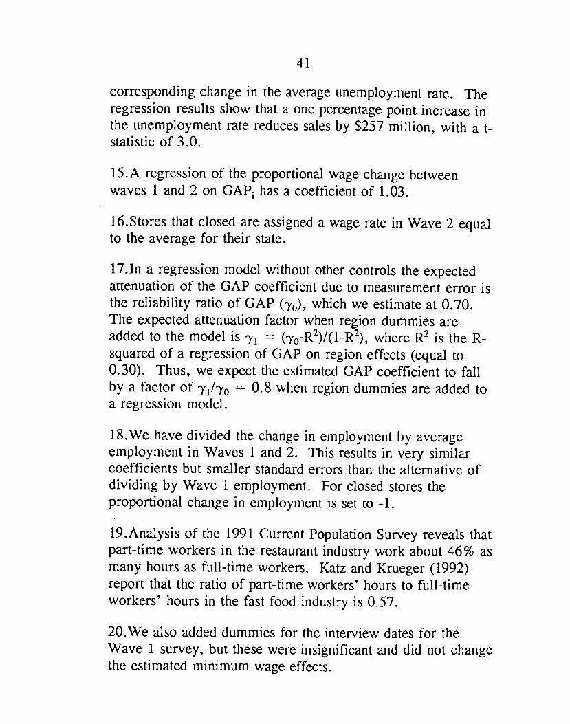
15.A regression of the proportional wage change betweenwaves 1 and 2 on GAP1 has a coefficient of 1.03.

16.Stores that closed are assigned a wage rate in Wave 2 equalto the average for their state.

17.In a regression model without other controls the expectedattenuation of the GAP coefficient due to measurement error isthe reliability ratio of GAP (yo), which we estimate at 0.70.The expected attenuation factor when region dummies areadded to the model is = (-y0-R2)/(1-R2), where R2 is the R-squared of a regression of GAP on region effects (equal to0.30). Thus, we expect the estimated GAP coefficient to fallby a factor of -/y = 0.8 when region dummies are added toa regression model.

18.We have divided the change in employment by averageemployment in Waves 1 and 2. This results in very similarcoefficients but smaller standard errors than the alternative ofdividing by Wave 1 employment. For closed stores theproportional change in employment is set to -1.

19.Analysis of the 1991 Current Population Survey reveals thatpart-time workers in the restaurant industry work about 46% asmany hours as full-time workers. Katz and Krueger (1992)report that the ratio of part-time workers' hours to full-timeworkers' hours in the fast food industry is 0.57.

20.We also added dummies for the interview dates for theWave 1 survey, but these were insignificant and did not changethe estimated minimum wage effects.

42

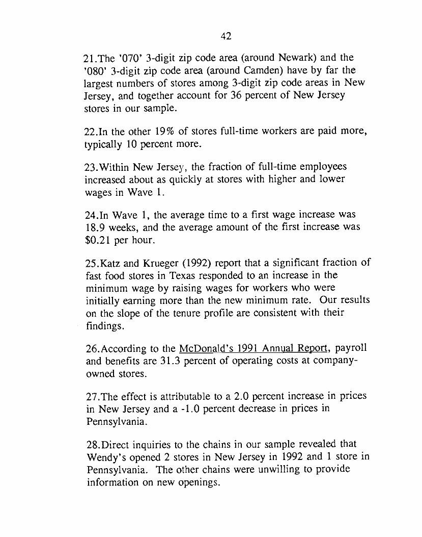
21.The '070' 3-digit zip code area (around Newark) and the'080' 3-digit zip code area (around Camden) have by far thelargest numbers of stores among 3-digit zip code areas in NewJersey, and together account for 36 percent of New Jerseystores in our sample.

22.In the other 19% of stores full-time workers are paid more,typically 10 percent more.

23.Within New Jersey, the fraction of full-time employeesincreased about as quickly at stores with higher and lowerwages in Wave 1.

24.In Wave 1, the average time to a first wage increase was18.9 weeks, and the average amount of the first increase was$0.21 per hour.

25.Katz and Krueger (1992) report that a significant fraction offast food stores in Texas responded to an increase in theminimum wage by raising wages for workers who wereinitially earning more than the new minimum rate. Our resultson the slope of the tenure profile are consistent with theirfindings.

26.According to the McDona'd's 1991 Annual Report, payrolland benefits are 31.3 percent of operating costs at company-owned stores.

27.The effect is attributable to a 2.0 percent increase in pricesin New Jersey and a -1.0 percent decrease in prices inPennsylvania.

28.Direct inquiries to the chains in our sample revealed thatWendy's opened 2 stores in New Jersey in 1992 and 1 store inPennsylvania. The other chains were unwilling to provideinformation on new openings.

43

29.We used the 1986 Current Population Survey mergedmonthly file to construct the minimum wage variables. Stateminimum wage rates in 1990 were obtained from Bureau ofNational Affairs (1990).

30.Sullivan (1989) and Ransom (1993) present empirical resultsfor nurses and university teachers that suggest monopsony-likebehavior of employers.

Per

cent

of

Sto

res

Per

cent

of

Sto

res

- hi

(a

(a

o

U.

0 U

C

(P

0

U

—

I I

I I

hi

(P

S

(a

0 U

I • C

•

—4-

U

. —

. S

. __

____

____

____

____

____

0

- '1

o

CD

0

• 0

CD

-

"I

C

0 0 -

CD

•1

—

—

'CD

—

.4-

- (I

D

—.

(D _

____

____

____

____

__

CL)

:

—

(0

o __

____

____

____

____

____

____

____

_ Is

N

-)

_ U

I hi

a

UI •

(0

(Il

CD

V

.

U.

(p

I,.

0 U

. —

4-.

CD

(1

)

—

PU

U

I •.

P

O

-

ID

0 0

0 0

0 0

0 0

0 0

D

ID 0 0 S

ID

lb

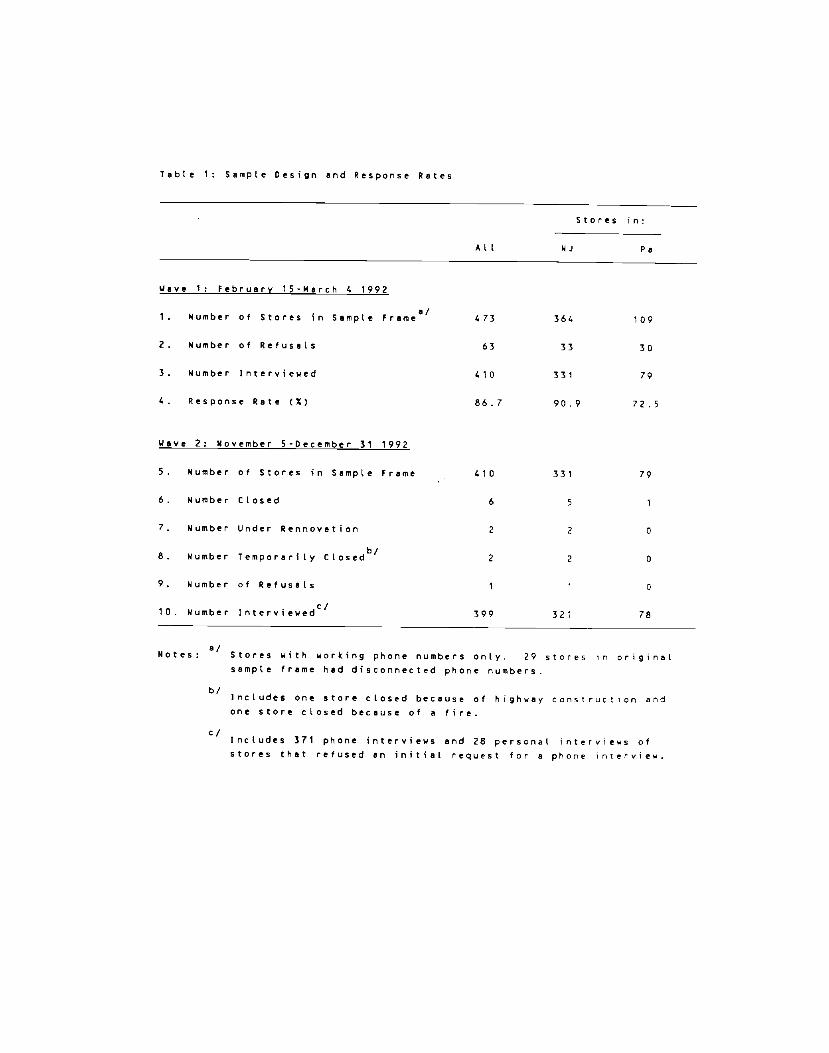
Table 1: Sample Design and Response Rates

Alt

Stores in:

NJ Pa

Wave 2: November 5

5. Number of Stor

6. Number Closed

7. Number

8. Number

9. Number

10. Number

410 331

6

2 2

2 2

399 321

79

0

0

0

78

Notes: Stores with working phone numbers onLy. 29

sample frame had disconnected phone numbers.

b/Includes one store closed because of highwayone store closed because of a fire.

ClIncludes 371 phone interviews and 28 personastores that refused an initial request for a

stores in original

construction and

I interviews ofphone Interview.

Wave 1: F

1. Numbe

2. Numbe

3. Numbe

4. Respo

a!

ebruary 15-March 4 1992

r of Stores in Sample Frame

r of Refusals

r Interviewed

rise Rate (X)

63 33 30

410 331 79

-December 31

es in Sample

1992

F reme

t ion

I osed'"

Under Rennova

Temporarily C

of Refusals

c/Interviewed

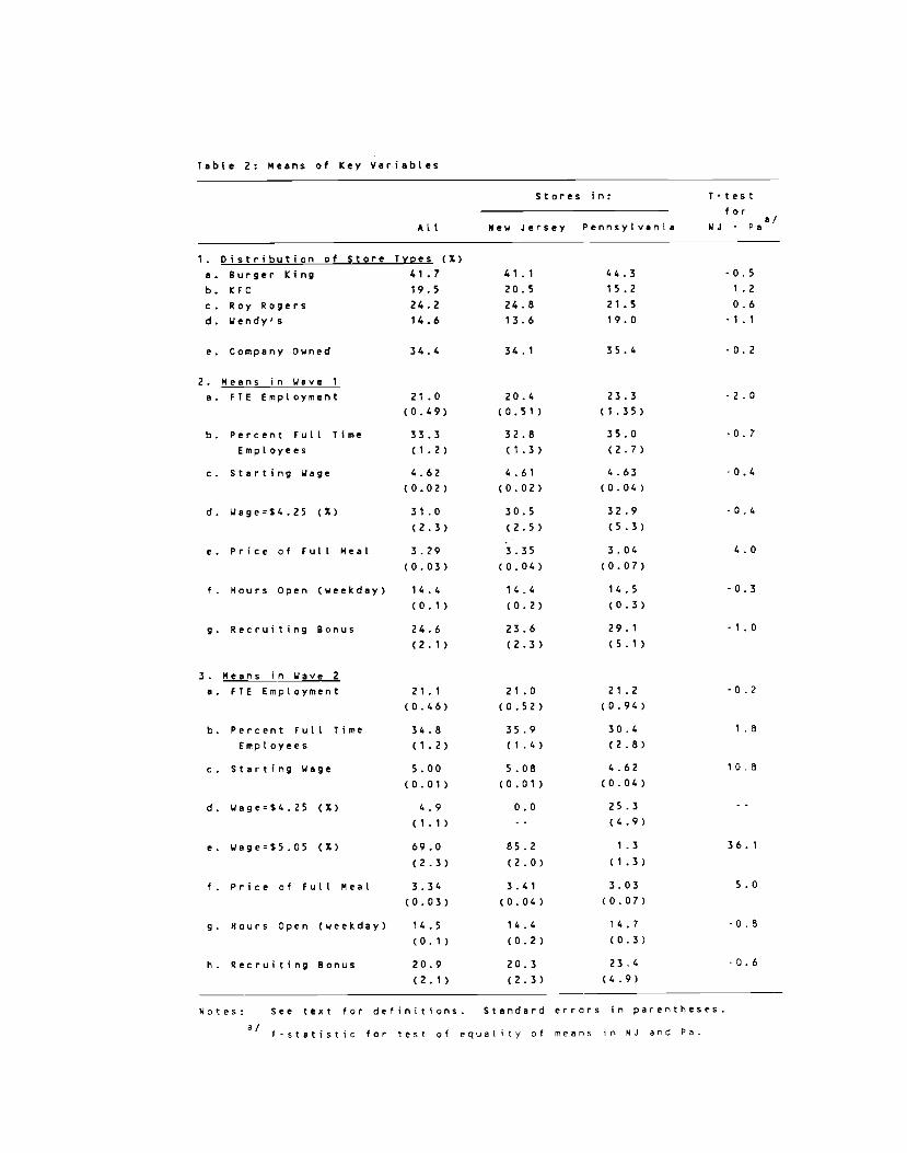
Table 2: Means of Key Variables

Stores

All New Jersey

in: 1-testfor

a!NJ - Pa.Pennsylvania

1. Distribution of Store types CX)a. Burger King 41.7 41.1 44.3 -0.5

b. KFC 19.5 20.5 15.2 1.2

c. Roy Rogers 24.2 24.8 21.5 0.6

d. Wendy's 14.6 13.6 19.0 -1.1

e. Company owned 34.4 34.1 35.4 -0.2

2. Means in Wave 1a- FIE EmpLoyment 21.0 20.4 23.3 -2.0

(0.49) (0.51) (1.35)

b. Percent Full Time 33.3 32.6 35.0 -0.7

EmpLoyees (1.2) (1.3) (2-7)

c. Starting Wage 4.62 4.61 4.63 -0.4

(0.02) (0.02) (0.04)

d. Wage=14.25 (U 31.0 30.5 32.9 -0.4

(2.3) (2.5) (5.3)e. Price of Full Meal 3.29 3.35 3.04 4.0

(0.03) (0.04) (0.07)

f. Hours Open (weekday) 14.4 14.4 14.5 0.3(0.1) (0.2) (0.3)

g. Recruiting Bonus 24.6 23.6 29.1 -1.0

(2.1) (2.3) (5.1)

3. Means in Wave 2a. FT 6 Employment 21 .1 21 .0 21 .2 -0.2

(0.46) (0.52) (0.94)

b. Percent Full Time 34.8 35.9 30.4 LBEmployees (1.2) (1.4) (2.8)

c. Starting Wage 5.00 5.08 4.62 10.8

(0.01) (0.01) (0.04)d. WagetS4.25 CX) 4.9 0.0 25.3 -

(1.1) (4.9)

e. Wage=S5.05 (X) 69.0 85.2 1.3 36.1(2.3) (2.0) (1.3)

f. Price of Full Meal 3.34 3.41 3.03 5.0

(0.03) (0.04) (0.07)

g. Hours Open (weekday) 14.5 14.4 14.7 -0.6

(0.1) (0.2) (0.3)Ii. Recruiting Bonus 20.9 20.3 234 -0.6

(2.1) (2.3) (4.9)

Notes: See text for definitions. Standard errors in parentheses.at .1-statistic for test of equaLIty of means in NJ and Pa.

Table 3: Average EnLoynent Per Store Before and After RISC in New Jersey Miniflun Wage

Alt

Stores By State:

Pa

NJ

Diff:

NJ-Pa

Stores in New Jersey

Di fferenceg

within NJ /

Low

Midrange

-High

-High

Wages

Wage

Wage

$425

4.26-4.99 5.00

1. FTE Enptoyment Before,

ALL Aaitabte Cbs.

21.00

(0.49)

23.33

(1.35)

20.44

(0.51)

-2.89

(1.44)

19.56

20.08

22.25

(0.77)

(0.84)

(1.14)

-2.69

-2.17

(1.37)

(1.41)

2. FTE teptoyment Af

ter,

AU Available Ob.

21.05

(0.46)

21.1?

(0.94)

21.03

(0.52)

-0.14

(1.07)

20.88

20.96

20.21

(1.01)

(0.76)

(1.03)

0.67

0.75

(1.44)

(1.27)

3. Change in Mean FT

EWloyment

0.05

(0.50)

-2.16

(1.25)

0.59

(0.54)

2.76

(1.36)

1.32

0.87

-2.04

(0.95)

(0.84)

(1.14)

3.36

2.91

(1.48)

(1.41)

4. Change in Mean FTE

Ento)ment, BeLaried

Sairple of S

toresC

-0.07

(0.66)

-2.28

(1.25)

0.47

(0.48)

2.75

(L34)

1.21

0.71

-2.16

(0.82)

(0.69)

(1.01)

3.36

2.7

(1.30)

(1.22)

5. Change in Mean FTE

ErrployTrlent, Setting

FIE at l

eirporarily

Closed Stores to 0

-0.26

(0.47)

-2.28

(1.25)

0.23

(0.49)

2.51

(1.35)

0.90

0.49

-2.39

(0.87)

(0.69)

(1.02)

3.29

2.88

(1.34)

(1.23)

Wotes: Standard errors in parentheses.

Sairple consists of all stores with non-missing data on eirployment. tIE (tuu-time

equivalent eirptoyment) counts each part-time worker as 1/2 a fuLL-time worker.

EurpLoymnt at 6 cLosed stores is

set to zero.

Eirployment at 4 tee,orariLy closed stores

is treated as missing.

a/Stores in New Jersey classified by whether starting wage in Wave I

equals $425 p

er hour (N101), is between

$4.26 and 5.6.99 per hour (N140), or is $5.00 per hour or higher (NT3).

b/Difference

in e ,loyment between stores in Low (5.4-25 per hour) arid high ('SSOO per hour) wage ranges;

arid difference in eiploent between stores in midrange ($4264.99 per hour) and high wage ranges.

C/Sset of stores with non-missing

eirç,loy,nent in Wave

1 and Wave 2.

d/10 this row Only, WSvt 2 eirptoyment at 4 teirporarily closed stores is set to 0.

Eirptoyment

changes are based on subset of stores with non-missing eoploynmnt in Wave ¶

arid Wave 2.

Tab

le 4

: R

educ

ed F

orm

Mod

els

for

Cha

nge

In Employment

Dependent

Var

iabl

e:

Cha

nge

in E

lplo

Ym

enta

/ Proportional

Cha

nge

in E

ITpl

Oym

entb

I'

(1)

12)

(3)

(4)

(5)

(6)

(7)

(8)

(9)

(10)

1.

New

Jersey Oum,y

2.33

(1.19)

2.30

(1.20)

--

- "

0.05

(0.05)

0.05

(0.05)

--

..

2. In

itial

Wag

e G

ap'

--

--

15.65

(6.08)

14.92

(6.21)

11.91

(7.39)

--

0.39

(0

.26)

0.

34

(0.2

6)

0.29

(0

.31)

3. Controls for )ain

and Ownership

no

yes

no

yes

yes

no

yes

no

yes

yes

4. Controls for Region

no

no

no

no

yes

no

no

no

no

yes

5.

Sta

ndar

d E

rror

of

Reg

ress

ion

8.79

8.78

8.

76

8.76

8.75

0.373

0.372

0.373

0.372

0.37

2

6.

Pro

babi

lity

V,u

e fo

r Controls

--

0.34

0.

44 .

0.40

--

0.

14

--

0.17

0.

27

Not

es:

Sta

ndar

d er

rors

in

par

enth

eses

. S

ampl

e co

nsis

ts o

f 35

7 st

ores

with

no

n-m

issi

ng d

ata

on e

mpl

oym

ent

anti

starting wages

in W

av.s

1

and

2.

All

mod

els

include an u

nres

tric

ted

cons

tant

(no

t reported).

a/D

epet

..45.

,t va

riabl

e is

change

in f

ull-t

ime

equi

vale

nt employment.

The mean and s

tand

ard

devi

atio

n of

the dependent

variable are -0.237 and 8.825, respectively.

b/oep._nt v

ariable is the change in full-time equivalent

empl

oym

ent,

divi

ded

by a

verage employment In Wave

I

and

Wav

e 2.

For closed stores proportional change

•1.0. The mean and standard deviation of the dependent variable are -0.005 and 0.374,

respectively.

C/proportional

increase

in starting wage necessary to r

aise

starting wage to new minim.mi rate.

For stores in

Peonsylvanlo the wage gap

is 0

.

varia

bles

for ch

ain

type (3) ar

4 w

heth

er o

r no

t the store

is c

oepar,y-owned are Included.

variables for 2 re

gion

s of New Je

rsey

and 2 re

gion

s of Eastern Pemsylvania are included.

'Probability v

alue of joint F-test for ex

clus

ion

of al

l co

ntro

l variables.

Table 5: Specification Tests of Reduced Form Employment Models

Change in

EmploymentProportional Change

Employment

in

NJ Dummy Gap MeasureNJ Dummy Gap Measure(1) (2) (3) (4)

1. Base Specification 2.30 14.92 0.05 0.34(1.19) (6.21) (0.05) (0.26)

2. Treat 4 Temporarily 2.20 14.42 0.04 0.34Closed Storas as (1.21) (6.31) (0.05) (0.27)Permanently Closad'

3. Exclude Managers in 2.34 14.69 0.05 0.28Employment Count

/(1.17) (6.05) (0.07) (0.34)

4. Weight Part-time/

2.34 ¶5.23 0.06 0.30as 0.4Ful Ntimec (1.20) (6.23) (0.06) (0.33)

S. weight Part-time 2.27 14.60 0.04 0.17as 0.6*FulHtime (1.21) (6.26) (0.06) (0.29)

6. txclude Stores in 2.58 16.88 0.06 0.42NJ Shore AreaC! (1.19) t6.36) (0.05) (0.27)

7. Add Controls for 2.27 15.79 0.05 0.40Wave? Interview (1.20) (6.24) (0.05) (0.26)Date

8. Exclude Stores 2.41 14.08 0.05 0.31Cal led More than, (1.28) (7.11) (0.05) (0.29)Twice in Wave

9. Weight by AnitiaL -- -- 0.13 0.81

Employment (0.05) (0.26)

10. Stores in Town, -- 33.75 -- 0.90around Newark' (16.75) (0.74)

11. Stores in Towns - 10.91 -. 0.21around Cambden (14.09) (0.70)

12. Pennlvania Stores - -0.30 -- -0.33Only (22.00) (0.74)

Notes: Standard errors in parentheses. Entries represent est matedcoefficient of New Jersey dummy (columns 1 and 3) or initialwage gap (columns 2 and 4) in regres ion models for the changein employment or the percentage change in employment. At I models

also include chain dummies and an indicator for company-ownedstores.

Notes for Table 5, continued

a/wave 2 empLoyment at 4 temporariLy cLosed stores Is set to 0 (rather

than missing).

b/FULL time equivalent employment excludes managers and assistant

managers.

c/Full time equivl ant employment equals number of managers, assistantmanagers, and full-time non-management workers, pLus 0.4 times thenumber of part-time non-management workers.

FuLL time equiviant empLoyment equaLs number of managers, assistantmanagers, and fulL-time non-management workers, pLus 0.6 times thenumber of part-time non-management workers.

c/sample excludes 35 stores Located in towns along the New Jerseyshore.

Models IncLude 3 dummy variables identifying week of Wave 2interview in November-December 1992.

excludes 70 stores (69 in NJ) that were contacted 3 or moretimes before obtaining Wave I interview.

h/Regression model is estimated by weighted Least squares, usingemployment in wave I as a weight.

'tsubsampLe of 51 stores in towns around Newark.

"SubsampLe of 54 stores in towns around Camden.

k/subsample of Pennsylvania stores only. wage gap is defined aspercentage increase in starting wage necessary to raise startingwage to 55.05.

Table 6: Effects of Minimum Wage Increase on Other Outcomes

Mean Regression of Chenge inChange in Outcome: Outcome Varab!e on:

NJ Pa NJ-Pa NJ Dummy lage Gap' ua;e Ca(I) (2) (3) (4) (5) (6)

OUTCOME MEASURE:

Store Characteristics

1. Fraction Ful I-Time 2.64 -4.65 7.29 730 33.64 2028.Workers CX) (1.71) (3.80) (4.17) (3.96) (20.95) (24.34)

7. Number of Hours -0.00 0.11 0.11 -0.11 -0.24 0.04Open per weekday (0.06) (0.08) (0.10) (0.12) (0.65) (0.76)

3. Number of Cash -0.04 0.13 -0.17 -0.18 -0.31 0.20Registers (0.04) (0. 10) (0.11) (0.101 (0.53) (0.67i

4. Number of Cash -0.03 -0.20 0.17 0.17 0.15 -0.47Registers Open (0.05) (0.08) (0.10) (0.12) (0.621 (0. 74)at 1100 am

Employee Meal Programs-

5. Low-Price Meal -4.67 -1.28 -3.39 -2.01 -30.31 -33.15Program CX) (7.65) (3.86) (4.68) (3.63) 129.00) (35.04

6. Free Meal 8.41 6.41 2.00 0.49 79.90 36.91Program (X) (2.17) (333) (3.97) (4.50) (23.75) l27.0)

7.Combination of low -4.04 -5.13 1.09 1.20 -11.57 -19.19Price and Free (1.98) (3.11) (3.69) (4.321 (22-57) (26.51Meals (X)

Wgp Prof lIe

8. time to First Raise 3.77 1.26 2.51 2.21 4.02 -5.17(weeks) (0.89) (1.97) (2.16) (2.03) (10.81) 1 12.7L'

9. utual Amount of -0.01 -0.02 0.01 0.01 0.03 7-01First Raise (cents) (0.01) (0.07) (0.02) (0.02) (0.1)) (0.11)

10. Slope of Wage -0.10 -0.11 0.01 0.J7) -0.02 -0.7-?

Profile (X per week) (0.04) (0.09) (0.10) (0. lOi (0.56) (0.57)

Notes: Entries in columns 1 and 2 represent mean changes in the outcome variableindicated by the row heading for stores with non-missing data on the outcomein Waves 1 and 2. Entries In columns 4-6 represent estimated regressioncoefficients of indicated variable (NJ dummy or initial wage gsp) in model forthe change in the outcome variable. Regression modets include chain dummies andan Indicator for company-owned stores.

Wage gap is proportional increase in starting wage necessary to raise wage tonew minimum rate. For stores in Pennsylvania, the wsge gap is zero.

Models in column 6 include dummies for 2 regions of New Jersey and 2 regionsof Eastern Pennsylvania.

c/Fraction of part-time employees in total full-time eguivslent employment.

1. Mew Jersey Dummy 0.033

(0.014)

2. nitial Wage oape/f

S. Standard Errorof Regression

0.101 0.097 0.102

b/Dummy variables for chain type (3) and whether or not store iscompany-owned are included.

C/Dummy variables for 2 regions of New Jersey and 2Pennsylvania are included.

Table 7: Reduced Form Models for Change in the Price of Full Meat

(1) (2) (3)

Dependent Variable: Change Log Price of Full Meat

(4) (5)

0.037(0.014)

0.077 0.146 0.063

3. Controls forCg,in

no yes no yes yesand Ownership

4. Controls for Region no

0.098 0.097

a/

Motes : Standard errors i n parent h as as . En t r t as a r e e 5 t is, a t it d r e g r e 5 5 i on

coefficients for modeLs fit to change in log price of a full treat

(entree, medium soda, small fries). The sample contains 315 storeswith valid data on prices, wages, and employmentThe mean and standard deviation of the dependent

for Waves 1variable are

and 2.

0.0173and 0.1017, respectiveLy.

ProportionaL increase in starting wage necessary to raise wage to newminimum rate. For stores in Pennsylvania the wage gap is 0.

regions of Easter"

Table 8: Estimated Effecs of Minimum Wages on Numbers of McDonald's Restaurants, 1956 to 1991

Dependent Variable: Proportional

Increase in Number of Stores

Oependen

Opened

t Variable: Number

Stores / Number inNewly

1956

(1) (2) (3) (4) (5) (6) (7) (8)

Minimum Wane Variabte:

1. Fraction of RetaiL Workers 0.33

in Affected Wage Range 1986a,' (0.20)

•- 0.13

(0.19)

-- 0.37

(0.22)

-. 0.16(0.21)

--

2. State Minimum Wage in 1991b - -/ Average Retail Wage 1986

"0.38 --

(0.22)0.47

(0.22)

- - 0.47 - -

1023)0.56

10.2')

Other Control Variables:-- -- 0.88

(0.23)

1.03

(0.23)

-- -- 0.86(0.25)

1.04

(0.25)

3. Proporsional Growth in

Population, 1986 to 1991

4. change in Unemployment

Rates, 1986 to 1991

-. -- -1.78(0.62)

-1.40

(0.61)

-- -- -1.85(0.68)

-L40(0.65)

5. Standard Error of 0.083 0.083 0.071 0.068 0.088 0.088 0.077 0.073

Regress i on

Notes: Standard errors in parentheses. Sample contains SI state-level observations (including D.C.)

on the number of McDonalds restaurants open in 1986 and 1991. Dependendent variable in columns

(1)-(4) is proportional increase in the number of ressaurants open. Mean and standard deviation

are .246 and .085, respectiveLy. Dependendent variable in columns (5)-IS) is ratio of the

number of new stores opened between 1986 and 1991 to the number open in 1986. Mean and standard

deviation are .293 and .091, respectively. All regressions are weighted by state population

in 1986.

Fraction of all workers in retail trade in the state in 1986 earning an hourly wage between

$3.35 per hour and the "effective" state minimum wage in 1990 (i.e., the maximimum o' the

Federal minimum wage in 1990 ($3.80) and the state minimum wage as of ApriL 1 1990).

Maximum of state and Federal minimum wage as of April 1 1990 divided by average hourLy wage

workers in retail trade in the state in 1986.

TabLe 9: EmpLoyment-Popu(aton Rates for Teenager-s and AdLts,

ApriL-December of 1991 and 1992

EmpLoyment-PopuLation Rate:

Change:

1991 1992 1992-1991

New Jersey

Teenagers 37.7 37.0 -0.7

(1.8) (1.8) (2.2)

Age 25 and OLder 64.1 61.5 -2.6

(0.5) (0.5) (0.6>

PennsyLvaniaTeenagers 48.0 45.3 -2.7

(1.0> (1.9> (2.3)

Age 25 and 0(der 58.8 59.1 0.3

(0.5) (0.5) (0.6)

New York

Teenagers 31.4 28.6 -

(1.3) (1.3) (1.6)

Age 25 and 0(der 59.6 58.6 -1.0

(0.4) (0.4) (0.5)

AU U.S.

Teenagers 43.5 42.4 -1.1

(0.4) (0.4) (0.5>

Age 25 and OLder 62.7 62.5 -0.2

(0.1) (0.1) (0.1>

Notes: Estimated standard errors in parentheses.

Estimated from monthLy Current Population Survey files for

ApriL-December of 1991 and 1992.