sugar plant simulator for energy management purposes · to test the optimization and replace the...

SUGAR PLANT SIMULATOR FOR ENERGY MANAGEMENT PURPOSES

Cristian Pablos a, L. Felipe Acebes b, Alejandro Merino c

(a)(b) Systems Engineering and Automatic Control Department, EII, University of Valladolid, C/ Real de Burgos s/n, 47011, Valladolid, Spain

(c)Electromechanical Engineering Department, University of Burgos, Av. Cantabria s/n, 09006 Burgos, Spain

(a)[email protected], (b)[email protected], (c)[email protected]

ABSTRACT This paper deals with the development of a simulator for energy purposes. The aim of the simulator is being used as a substitute of a real sugar plant in a testing phase of a Real Time Optimization system for the management of the power energy in the plant, and the use of steam in the process. An Equation Based Object Oriented Language (EBOOL) has been used, so different models of each part of the production process have been modelled separately and then joined together to build the final model. To do so, first principle models are combined with others based on experience depending on the accuracy needed, in order to maintain always equilibrium with computing performance. Several tests, changing between different operational points were performed with the simulator to verify its robustness and performance, and to check if it is suitable to be used by the optimization system.

Keywords: Sugar factory simulator, CHP plant, Grey Box Modeling, Energy optimization.

1. INTRODUCTION Nowadays, while the complete development of renewable energies is hoped, cogeneration, which can be defined as the simultaneous generation of heat and power, has raised as a very important candidate to energy production in industrial processes. The high efficiency inherent to this process makes possible to save money reducing the amount of fuel used to obtain energy in comparison with conventional plants. Furthermore, this feature also implies a reduction in emissions, something that is very interesting as global leaders are putting their attention on new laws to stop global warming. As a production point of view, it also provides more security in the supply of heat and power energy to the process, so it can be very interesting study how processes associated with this type of technology can be optimized (Tina, G.M. Passarello G. 2012). One problem related to this type of processes is that changes in energy prices, and restrictions in the way energy can be obtained makes them compulsory to be operated in real time. However, due to the amount of variables involved, it is very hard to find the optimum

operational point which gives the maximum profits. Different approaches have been found trying to solve a problem where the energy costs wanted to be optimized in non-related industrial processes applications, such as district heating systems (Ristic M. et al. 2008) or power plants based on this technology (Mitra S. et al. 2013), (Sanaye S. and Nasab A.M. 2012). Other studies put their attention on petrochemical or other type of industries where the production is fixed and hence the power and heat demand (Ashok S., Banarjee R. 2003). However, few studies consider the possibility of changing the production in order to reduce the energy costs and make more profit. To solve this problem a RTO (Real Time Optimization) System (Darby M.L. et al. 2011) has been thought to help managing the production, taking into account considerations aspects like the possibility of selling or buying power energy to the external grid. As case study, a sugar process industry has been selected because of its traditional relationship with cogeneration and the extensive experience of the working team with this type of process industry. Tools based on optimization must be proved on simulation before trying them on real processes plants. This way, security and production problems can be avoided saving time and money. Taking this into account, the global problem can be divided in two main parts. On the one hand, the optimization problem has to be study deeply in order to understand the different variables and aspects that take place. The formulation of the problem is a key part in the development of the global work, therefore different approaches and optimization strategies must be studied. On the other hand, a sugar plant dynamic simulator focused on energy aspects has to be modelled in order to test the optimization and replace the real sugar plant. This simulator will be also useful to study the process, and make experiments related to the effect that different key variables may have in energy consumption and management. Previously, the working team developed a complete sugar factory simulator for operators training (Merino A., et al 2009). Nevertheless, because of the complexity of the models used, the simulation can

Proceedings of the European Modeling and Simulation Symposium, 2017 ISBN 978-88-97999-85-0; Affenzeller, Bruzzone, Jiménez, Longo and Piera Eds.

370

mailto:[email protected]



hardly run faster than real time, which makes very difficult carry out tests in an agile way. Furthermore, as was aforementioned this simulator is focused on training operators, so the process is not completely automated and the simulation cannot run without human intervention. Besides, the simulator does not include the beet storage and the factory power demands. All this problems makes recommended the construction of a new simulator based on the previous one, complex enough to represent the behaviour of the global process, but simpler and faster. So the objective of this work is the development of that simulator and perform tests in order to analyse whether it can be

applied as a replacement of the complete sugar factory in the RTO system. The rest of this paper is organised as follows: In the second section, a description of typical beet sugar process is given to help to understand the different parts of this process and the most important variables associated. Next, the third section deal with the plant mathematical model and its implementation to perform the simulator. Later, some simulation tests are shown to demonstrate the simulator features, and finally some conclusions are stated.

Figure 1. Simplified schematic of a typical sugar factory with a CHP plant

2. SYSTEM OVERVIEW The manufacturing of raw sugar from beets is a highly technical process which requires large and costly manufacturing equipment. A typical beet-sugar factory is divided into two sections: beet-end or raw-side and sugar end or refinery-side (Asadi M., 2007). Besides, steam boilers and steam turbines are necessary to produce low pressure steam and electricity. Figure 1 shows a simplified block diagram of the production. The factory takes delivery of the beets through lorries, which are unloaded and beets are piled and stored in beet-storage areas. The storage time is an important variable that affects sugar contain-reduction of the beets due to the beet respiration and microorganism. Other important constraint is the available surface of the storage areas. So, these issues affects to the beet feeding to the factory.

The production process begins when the beet is washed and cut to obtain thin slices called cossettes. In the diffusion section, cossettes are contacted with hot water flowing countercurrently to extract the sucrose from them and the diffusion juice is obtained. This process is carried out into the diffuser, whose electrical drives are one of the main power consumers of the factory. The pulp, or sugar-exhausted cossettes, is compressed, dried and processed as animal feed. The pulp presses are other important power consumers. In the purification section, the diffusion juice is heated and lime added to control the juice pH. After two carbonation process, the juice impurities are removed by filtration and the obtained clear or purified juice is used to feed the evaporation section.

SUGAR-END

BEET-END

Vapor

Natural Gas HP Steam Electricity


371

In the diffusion and purification sections the main steam consumption is due to the heat exchangers that heats the different juices. The clear juice feed the evaporation section which purpose is to remove part of the water in the juice, increasing its Brix, or percentage of dry substance, to obtain syrup. This process is carried out in a multiple-effect evaporation, in which the juice is boiled in a sequence of vessels. The first vessel (at the highest pressure) requires steam from turbines and the vapor boiled off in each vessel is used to heat the next as well as to feed other steam consumers of the factory. So, this section is the largest steam consumer of the factory. The obtained syrup feeds the sugar-end, where sucrose is crystallized to obtain granulated-refined sugar and molasses (a by-product). The process is divided in three stages, in each stage vacuum pans are used to crystallized the sucrose and, later, centrifuges separate the sugar crystals from honeys. The commercial sugar is obtained in the first stage, the next ones are recovery stages to minimize the sugar losses. The sugar-end is very complex to operate, because the majority of crystallizers and centrifuges are batch process units, and the product storage capacity is limited. Crystallizers are the greatest consumers of the evaporation steam, and, together with the centrifuges, consume a lot of power. Besides, as they are batch units these demands are discontinuous in time and magnitude. To supply the demands of steam and power, the factory disposes of a cogeneration, or combined heat and power (CHP), plant. Using natural gas, or other fuel, boilers generate high pressure steam that is sent to steam turbines to generate electricity, and low-pressure steam for the evaporation section. The CHP plant is working to produce the steam and power that the factory needs. But, sometimes, there will be available power to sell, and other times it will be necessary to buy power to the electrical companies. After this description, it is easy to imagine that a sugar factory is a good example to schedule the production, keeping in mind the prices of the fuels and power, the deliveries of sugar beets and the storage capacity of the factory. So, in order to test different kinds of scheduling strategies it is necessary to dispose of a good simulator to replace a real factory. 3. MODELING AND SIMULATION

3.1. Modeling and simulation environment It is well known that the first stage of a simulation project is to establish the simulation aims. In this case, the final objective is to have a dynamic and realistic simulation of a well-defined industrial process to obtain a set of experimental data to identify reduced models of the system, develop a RTO algorithm, and test the

implementation of the RTO in an industrial control system. As scenarios of several days of length must be simulated, it is necessary a simulator simple enough to carry out a lot of experiments with short computing time. However, an excess on simplification can lead to a problem related to lack of accuracy, so it must be managed an equilibrium between accuracy and computation time. Then, the mathematical model must be a first principles dynamic one, but in case the difficulty of the model exceeds the intended use, sufficiently validated empirical relations will be used. This implies that the formulation of the model must be based on ODEs, DAEs, algebraic equations, tables and events. Given the magnitude of the system to be simulated, its mathematical model must be developed incrementally, using models that can be instantiated from a library and composed in a hierarchical way. A requirement for the simulation tool is the capacity to develop model libraries from scratch. Although using commercial libraries can be helpful sometimes, since a gain in time and no errors are expected, sometimes they limit the characterization of the simulated process and in certain cases, like the sugar industry, these libraries does not exist. Another requirement is that the modeling tool should help in the task of symbolic manipulation of the global mathematical model to obtain in an easier way the simulation model based on the input variables. These requirements imply to choose a modeling environment that implements an equation object oriented modeling language (EOOBML), and a graphical interface that allows the modeling based on the connection of components. The modeling environment must be linked to a simulation environment that facilitates model execution, changes in parameter and input signals, and visualization of output signals. Also, it must allow the recording of the results, so that the data can be exploited with another tools. The simulation must be able to be used standalone the modeling and simulation environment. In particular, it is desired to use a modeling and simulation environment that allows to obtain standalone simulators with OPC (OLE for Process Control) connectivity, since OPC is supported by industrial control systems and by other tools such as MATLAB. So, the modeling and simulation environment selected is EcosimPro (EA Internacional 2017), since it disposes of the aforementioned specifications. In particular, its modeling language shares many characteristics with languages based on Modelica (Modelica Association et al 2017).


372

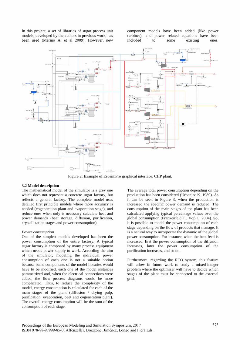
In this project, a set of libraries of sugar process unit models, developed by the authors in previous work, has been used (Merino A. et al 2009). However, new

component models have been added (like power turbines), and power related equations have been included to some existing ones.

Figure 2: Example of EsosimPro graphical interface. CHP plant.

3.2 Model description The mathematical model of the simulator is a grey one which does not represent a concrete sugar factory, but reflects a general factory. The complete model uses detailed first principle models where more accuracy is needed (cogeneration plant and evaporation stage), and reduce ones when only is necessary calculate heat and power demands (beet storage, diffusion, purification, crystallization stages and power consumption). Power consumption One of the simplest models developed has been the power consumption of the entire factory. A typical sugar factory is composed by many process equipment which needs power supply to work. According the aim of the simulator, modeling the individual power consumption of each one is not a suitable option because some components of the model libraries would have to be modified, each one of the model instances parametrized and, when the electrical connections were added, the flow process diagrams would be more complicated. Thus, to reduce the complexity of the model, energy consumption is calculated for each of the main stages of the plant (diffusion / drying pulp, purification, evaporation, beet and cogeneration plant). The overall energy consumption will be the sum of the consumption of each stage.

The average total power consumption depending on the production has been considered (Urbaniec K. 1989). As it can be seen in Figure 3, when the production is increased the specific power demand is reduced. The consumption of the main stages of the plant has been calculated applying typical percentage values over the global consumption (Frankenfeld T., Voβ C. 2004). So, it is possible to model the power consumption of each stage depending on the flow of products that manage. It is a natural way to incorporate the dynamic of the global power consumption. For instance, when the beet feed is increased, first the power consumption of the diffusion increases, later the power consumption of the purification increases, and so on. Furthermore, regarding the RTO system, this feature will allow in future work to study a mixed-integer problem where the optimizer will have to decide which stages of the plant must be connected to the external grid.


373

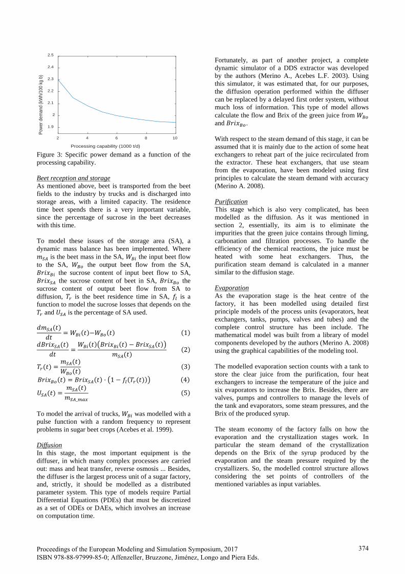
Figure 3: Specific power demand as a function of the processing capability. Beet reception and storage As mentioned above, beet is transported from the beet fields to the industry by trucks and is discharged into storage areas, with a limited capacity. The residence time beet spends there is a very important variable, since the percentage of sucrose in the beet decreases with this time. To model these issues of the storage area (SA), a dynamic mass balance has been implemented. Where 𝑚𝑚𝑆𝑆𝑆𝑆 is the beet mass in the SA, 𝑊𝑊𝐵𝐵𝐵𝐵 the input beet flow to the SA, 𝑊𝑊𝐵𝐵𝐵𝐵 the output beet flow from the SA, 𝐵𝐵𝐵𝐵𝐵𝐵𝐵𝐵𝐵𝐵𝐵𝐵 the sucrose content of input beet flow to SA, 𝐵𝐵𝐵𝐵𝐵𝐵𝐵𝐵𝑆𝑆𝑆𝑆 the sucrose content of beet in SA, 𝐵𝐵𝐵𝐵𝐵𝐵𝐵𝐵𝐵𝐵𝐵𝐵 the sucrose content of output beet flow from SA to diffusion, 𝑇𝑇𝑟𝑟 is the beet residence time in SA, 𝑓𝑓𝑙𝑙 is a function to model the sucrose losses that depends on the 𝑇𝑇𝑟𝑟 and 𝑈𝑈𝑆𝑆𝑆𝑆 is the percentage of SA used. 𝑑𝑑𝑚𝑚𝑆𝑆𝑆𝑆(𝑡𝑡)

𝑑𝑑𝑡𝑡= 𝑊𝑊𝐵𝐵𝐵𝐵(𝑡𝑡)−𝑊𝑊𝐵𝐵𝐵𝐵(𝑡𝑡) (1)

𝑑𝑑𝐵𝐵𝐵𝐵𝐵𝐵𝐵𝐵𝑆𝑆𝑆𝑆(𝑡𝑡)𝑑𝑑𝑡𝑡

=𝑊𝑊𝐵𝐵𝐵𝐵(𝑡𝑡)�𝐵𝐵𝐵𝐵𝐵𝐵𝐵𝐵𝐵𝐵𝐵𝐵(𝑡𝑡) − 𝐵𝐵𝐵𝐵𝐵𝐵𝐵𝐵𝑆𝑆𝑆𝑆(𝑡𝑡)�

𝑚𝑚𝑆𝑆𝑆𝑆(𝑡𝑡) (2)

𝑇𝑇𝑟𝑟(𝑡𝑡) =𝑚𝑚𝑆𝑆𝑆𝑆(𝑡𝑡)𝑊𝑊𝐵𝐵𝐵𝐵(𝑡𝑡)

(3)

𝐵𝐵𝐵𝐵𝐵𝐵𝐵𝐵𝐵𝐵𝐵𝐵(𝑡𝑡) = 𝐵𝐵𝐵𝐵𝐵𝐵𝐵𝐵𝑆𝑆𝑆𝑆(𝑡𝑡) · �1 − 𝑓𝑓𝑙𝑙(𝑇𝑇𝑟𝑟(𝑡𝑡))� (4)

𝑈𝑈𝑆𝑆𝑆𝑆(𝑡𝑡) =𝑚𝑚𝑆𝑆𝑆𝑆(𝑡𝑡)𝑚𝑚𝑆𝑆𝑆𝑆_𝑚𝑚𝑚𝑚𝑚𝑚

(5)

To model the arrival of trucks, 𝑊𝑊𝐵𝐵𝐵𝐵 was modelled with a pulse function with a random frequency to represent problems in sugar beet crops (Acebes et al. 1999). Diffusion In this stage, the most important equipment is the diffuser, in which many complex processes are carried out: mass and heat transfer, reverse osmosis ... Besides, the diffuser is the largest process unit of a sugar factory, and, strictly, it should be modelled as a distributed parameter system. This type of models require Partial Differential Equations (PDEs) that must be discretized as a set of ODEs or DAEs, which involves an increase on computation time.

Fortunately, as part of another project, a complete dynamic simulator of a DDS extractor was developed by the authors (Merino A., Acebes L.F. 2003). Using this simulator, it was estimated that, for our purposes, the diffusion operation performed within the diffuser can be replaced by a delayed first order system, without much loss of information. This type of model allows calculate the flow and Brix of the green juice from 𝑊𝑊𝐵𝐵𝐵𝐵 and 𝐵𝐵𝐵𝐵𝐵𝐵𝐵𝐵𝐵𝐵𝐵𝐵. With respect to the steam demand of this stage, it can be assumed that it is mainly due to the action of some heat exchangers to reheat part of the juice recirculated from the extractor. These heat exchangers, that use steam from the evaporation, have been modeled using first principles to calculate the steam demand with accuracy (Merino A. 2008). Purification This stage which is also very complicated, has been modelled as the diffusion. As it was mentioned in section 2, essentially, its aim is to eliminate the impurities that the green juice contains through liming, carbonation and filtration processes. To handle the efficiency of the chemical reactions, the juice must be heated with some heat exchangers. Thus, the purification steam demand is calculated in a manner similar to the diffusion stage. Evaporation As the evaporation stage is the heat centre of the factory, it has been modelled using detailed first principle models of the process units (evaporators, heat exchangers, tanks, pumps, valves and tubes) and the complete control structure has been include. The mathematical model was built from a library of model components developed by the authors (Merino A. 2008) using the graphical capabilities of the modeling tool. The modelled evaporation section counts with a tank to store the clear juice from the purification, four heat exchangers to increase the temperature of the juice and six evaporators to increase the Brix. Besides, there are valves, pumps and controllers to manage the levels of the tank and evaporators, some steam pressures, and the Brix of the produced syrup. The steam economy of the factory falls on how the evaporation and the crystallization stages work. In particular the steam demand of the crystallization depends on the Brix of the syrup produced by the evaporation and the steam pressure required by the crystallizers. So, the modelled control structure allows considering the set points of controllers of the mentioned variables as input variables.

2 4 6 8 10

Processing capability (1000 t/d)

1.9

2

2.1

2.2

2.3

2.4

2.5

Powe

r dem

and

(kW

h/10

0 kg

b)


374

Crystallization According to the previous description of the production process, the detailed modeling of the crystallization section requires a lot of batch process units. Besides, a right modeling of the process of formation of sugar crystals is quite complicated and it requires the use of models of population balances. Also, it is complicated the detailed modeling of the separation, by centrifugation, of sugar crystals from honeys. In previous work these problems were studied thoroughly (Mazaeda R. 2012) and the simulators had a high computational load. So, according to the aims of the simulator, a simplified model of this section has been developed. This model calculates the average steam demand of the crystallization as a function of the Brix and flow of syrup produced by the evaporation and the steam pressure to crystallizers: 𝑊𝑊𝑆𝑆𝑆𝑆(𝑡𝑡) = 𝐾𝐾 · 𝑊𝑊𝑠𝑠𝑠𝑠𝑟𝑟(𝑡𝑡) · 100−𝐵𝐵𝑟𝑟𝐵𝐵𝑚𝑚𝑠𝑠𝑠𝑠𝑠𝑠

100· 𝐻𝐻𝑠𝑠𝑠𝑠(1.5)𝐻𝐻𝑠𝑠𝑠𝑠(𝐵𝐵𝐵𝐵𝐵𝐵𝑙𝑙𝐵𝐵𝐵𝐵𝐵𝐵 𝑃𝑃𝑟𝑟𝑃𝑃𝑠𝑠𝑠𝑠𝑃𝑃𝑟𝑟𝑃𝑃) (6)

Where:

• 𝑊𝑊𝑆𝑆𝑆𝑆: average steam mass flow demanded by crystallization

• 𝑊𝑊𝑠𝑠𝑠𝑠𝑟𝑟: syrup mass flow • 𝐵𝐵𝐵𝐵𝐵𝐵𝐵𝐵𝑠𝑠𝑠𝑠𝑟𝑟: Syrup Brix • 𝐻𝐻𝑠𝑠𝑠𝑠: Enthalpy of saturated steam at a

determined pressure

The value of the K parameter was obtained by experimentation using the detailed simulator of crystallization previous cited. Additionally, a first order dynamic is added to the previous calculated average value. Finally, as the steam demand of the crystallization depends on the cycle time of the crystallizers, to make a more realistic approach, some negative and positive pulses have been added to the average value. The magnitude and frequency of pulses can be selected from the simulator. Cogeneration In the cogeneration station is where the steam and power demanded by the factory are produced. Due to its importance, the CHP plant has been modelled with the same method than the evaporation stage. This CHP plant mainly consists of boilers where steam is produced by heating water using the energy obtained from the combustion of some kind of fuel, and turbines where steam is expanded to obtain power energy. As showed in Figure 2 in our process this stage is formed by three boilers which can use natural gas or fuel-oil as fuel. There are also three different backpressure steam turbines where electric power is obtained. Apart from this, steam can pass through a bypass from the boilers directly to the evaporation section, this is the usual configuration in real plants. To protect the evaporation from huge steam pressure, a relief valve has been

modelled. The amount of steam which passes through the bypass and the relief valve is the manipulated variable of the controller that assures a determined steam pressure in the evaporation first effect. The model used to represent the behaviour of the boilers is very complex and based in first principles (Pelayo S. 1999). Mainly, besides the steam generator, it considers a preheating of the feed water before entering in the boiler, a superheating of the steam obtained through heat exchangers fed by the combustion fumes, and the typical control system of boilers. Regarding the turbines, the objective of this model is to simulate the steam expansion and the conversion of its thermal energy into electric power. Furthermore it is necessary simulate the possibility of sending power to the external grid or generating completely the amount of power demanded by the factory. If the CHP plant produces the power demanded by the factory, the turbines control system must assure that the rotational speed of each turbine axis is constant and equal to 50 Hz. However, if the CHP plant is connected to the external grid, the controlled variable is the generated power. Both cases, the steam flow which is expanded in the turbine is the controlled variable. Hence, the turbine model must represent not only the power generation, but also the rotational speed of the turbine. The model is based on the papers of (Thomas P. 1999) and (Chaibakhsh A., Ghaffari A. 2008), and on a library of thermodynamic properties of the steam (Merino A. 2008). 3.3 Simulator size The great order of magnitude of the simulator can be estimated taking into account that it is formed by 6485 equations, being 449 of those dynamic and 7 algebraic. Furthermore, it counts with 2131 parameters and 29 boundaries. A test was carried out to measure the simulation speed. In this test 48 h (172000 s) of production were simulated, changing between different operational points. The real time used by the simulation was 274 s, so a time ratio between simulation and real time of 628 was obtained. As inputs of the model, changes in the production and in the syrup Brix obtained from evaporation were considered. As outputs, besides of different operational variables related to the process, others associated with energy consumption were selected, as heat and power demand, cogeneration performance, fuel consumption… It is noteworthy that all the control system of the process has been modelled in detail, so changes in the inputs lead to new stationary points without human intervention, which will be very useful in future work with the RTO system.


375

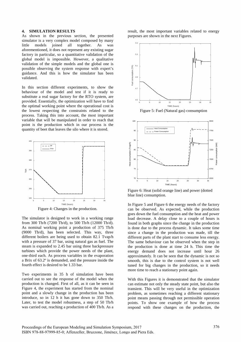
4. SIMULATION RESULTS As shown in the previous section, the presented simulator is a very complex model composed by many little models joined all together. As was aforementioned, it does not represent any existing sugar factory in particular, so a quantitative validation of the global model is impossible. However, a qualitative validation of the simple models and the global one is possible observing the system response with expert’s guidance. And this is how the simulator has been validated. In this section different experiments, to show the behaviour of the model and test if it is ready to substitute a real sugar factory for the RTO system, are provided. Essentially, the optimization will have to find the optimal working point where the operational cost is the lowest respecting the constraints related to the process. Taking this into account, the most important variable that will be manipulated in order to reach that point is the production which in our process is the quantity of beet that leaves the silo where it is stored.

Figure 4: Changes in the production.

The simulator is designed to work in a working range from 300 Tb/h (7200 Tb/d), to 500 Tb/h (12000 Tb/d). As nominal working point a production of 375 Tb/h (9000 Tb/d), has been selected. This way, three different boilers are being used to obtain 82.1 Tvap/h with a pressure of 37 bar, using natural gas as fuel. The steam is expanded to 2.45 bar using three backpressure turbines which provide the power needs of the plant, one-third each. As process variables in the evaporation a Brix of 63.2º is demanded, and the pressure inside the fourth effect is desired to be 1.33 bar. Two experiments in 35 h of simulation have been carried out to see the response of the model when the production is changed. First of all, as it can be seen in Figure 4, the experiment has started from the nominal point and a slowly change in the production has been introduce, so in 12 h it has gone down to 350 Tb/h. Later, to test the model robustness, a step of 50 Tb/h was carried out, reaching a production of 400 Tb/h. As a

result, the most important variables related to energy purposes are shown in the next Figures.

Figure 5: Fuel (Natural gas) consumption

Figure 6: Heat (solid orange line) and power (dotted blue line) consumption. In Figure 5 and Figure 6 the energy needs of the factory can be observed. As expected, while the production goes down the fuel consumption and the heat and power load decrease. A delay close to a couple of hours is found in both graphs since the change in the production is done due to the process dynamic. It takes some time since a change in the production was made, till the different parts of the plant start to consume less energy. The same behaviour can be observed when the step in the production is done at time 24 h. This time the energy demand does not increase until hour 26 approximately. It can be seen that the dynamic is not so smooth, this is due to the control system is not well tuned for big changes in the production, so it needs more time to reach a stationary point again. With this Figures it is demonstrated that the simulator can estimate not only the steady state point, but also the transient. This will be very useful in the optimization problem, as sometimes reaching a different stationary point means passing through not permissible operation points. To show one example of how the process respond with these changes on the production, the

0 5 10 15 20 25 30 35

TIME (hours)

345

355

365

375

385

395

405

Tb/h

SP

SVar

0 5 10 15 20 25 30 35

TIME (hours)

4.5

4.7

4.9

5.1

5.3

5.5

Fuel

con

sum

ptio

n (T

/h)

0 5 10 15 20 25 30 35

TIME (hours)

70

75

80

85

90

95

100

Hea

t con

sum

ptio

n (T

vap/

h)

6500

6750

7000

7250

7500

7750

8000

Pow

er c

onsu

mpt

ion

(kW

)

Heat Consumption

Power Consumption


376

signal output of the pressure split range controller, which was mentioned in section 3.2 when the cogeneration was described (see Figure 7), has been selected.

Figure 7: Relief and bypass valve response to changes in the production Due to a decrease in energy needs when the production is reduced, it can be seen how the controller firstly tries to maintain the pressure closing the bypass valve to not disturb the turbines performance. As this is not enough, when the production is too low the controller has to open the relief valve and throw steam to the atmosphere. In this situation, the heat load of the plant is not sufficient to accomplish the power needs, and since the process is not connected to the external grid, turbines must supply the entire power demand. Therefore, the excess of steam must be released to the atmosphere to protect the evaporation from an increase in the working pressure. Obviously, this will not be a desire operational point. When the production is increased to 400 Tb/h the opposite behaviour is seen, now the relief valve must be closed and the bypass valve open. This is due to the fact that now the heat demand is greater than the one steam turbines need to generate the power required.

Figure 8: Specific heat (red solid line) and power (black solid line) consumption.

In Figure 8 the specific heat and power consumption of the entire factory can also be analysed and seen how linear it is to changes in the production. In the starting point, the specific power consumption is 19.5 kWh/Tb, which is close to the average value of 20 kWh/Tb found in (Frankenfeld T., Voβ C. 2004) for a typical sugar factory. Regarding the specific heat consumption, it can be observed that it is close to 0.22 Tvap/Tb, so it is between the typical limits for this type of industry, 0.2-0.22 Tvap/Tb, found in (Van der Poel P.W. et al 1998). As the production decreases, both heat and power specific consumptions grow a little. However, when the stationary point is reached it can be observed in Figure 8 that heat and power specific consumptions are almost the same as in the beginning. Only steam specific consumption increases a little because some steam is being thrown to the atmosphere as it can be seen in Figure 7. When the production increases, both the specific power and steam consumption decrease a lot in the transitory state because of the delay inherent to the system, but when the stationary state is reached it can be observed in Figure 8 that the specific power is essentially the same again. This indicates that the relationship between heat and steam specific consumption and production is linear. Finally, in Figure 9 it is showed how typical performance parameters for cogeneration plants can be evaluated using the simulator. The global efficiency (𝜂𝜂𝐺𝐺) is defined as how much useful heat (𝑄𝑄𝑃𝑃) and power (𝑊𝑊) are being obtained instantaneously from the combustion of natural gas (𝐹𝐹).

𝜂𝜂𝐺𝐺 =𝑄𝑄𝑃𝑃 + 𝑊𝑊

𝐹𝐹 (7)

Typical values for this coefficient on cogeneration systems with backpressure turbines are between 80 – 90%. In our starting point, a global efficiency is closed to 91.5 %, which is almost constant until the 9th hour when the relief valve is opened and the coefficient starts to decrease. This can be explained since the useful heat has been defined as the steam used by the process, the evaporation in our case. Because more fuel has to be burned in order to obtain steam that is not being used in the evaporation, the global efficiency of the process decreases. When the production is increased, values around 91.5% are obtained again. This behaviour can be explained in a better way observing the power (𝜂𝜂𝑃𝑃) and thermal (𝜂𝜂𝑡𝑡) efficiency separately, and taking into account that the sum of them yields the global performance defined on the previous equation.

𝜂𝜂𝑃𝑃 =𝑊𝑊𝐹𝐹

(8)

𝜂𝜂𝑡𝑡 =𝑄𝑄𝑈𝑈𝐹𝐹

(9)

0 5 10 15 20 25 30 35

TIME (hours)

0

1

2

3

4

5

6

Tv/h

Relief

Bypass

0 5 10 15 20 25 30 35

TIME (hours)

17

17.5

18

18.5

19

19.5

20

Spec

ific

Pow

er c

onsu

mpt

ion

(kW

h/Tb

)

0.18

0.2

0.22

0.24

Spec

ific

Hea

t con

sum

ptio

n (T

vap/

Tb)

Specific Power Consumption

Specific Heat Consumption


377

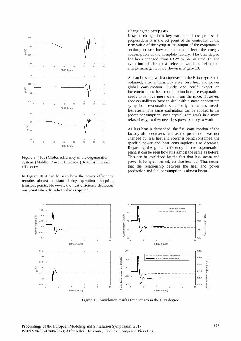
Figure 9: (Top) Global efficiency of the cogeneration system. (Middle) Power efficiency. (Bottom) Thermal efficiency. In Figure 10 it can be seen how the power efficiency remains almost constant during operation excepting transient points. However, the heat efficiency decreases one point when the relief valve is opened.

Changing the Syrup Brix Now, a change in a key variable of the process is proposed, as it is the set point of the controller of the Brix value of the syrup at the output of the evaporation section, to see how this change affects the energy consumption of the complete factory. The brix degree has been changed from 63.2° to 66° at time 1h, the evolution of the most relevant variables related to energy management are shown in Figure 10. As can be seen, with an increase in the Brix degree it is obtained, after a transitory state, less heat and power global consumption. Firstly one could expect an increment in the heat consumption because evaporation needs to remove more water from the juice. However, now crystallizers have to deal with a more concentrate syrup from evaporation so globally the process needs less steam. The same explanation can be applied to the power consumption, now crystallizers work in a more relaxed way, so they need less power supply to work. As less heat is demanded, the fuel consumption of the factory also decreases, and as the production was not changed but less heat and power is being consumed, the specific power and heat consumptions also decrease. Regarding the global efficiency of the cogeneration plant, it can be seen how it is almost the same as before. This can be explained by the fact that less steam and power is being consumed, but also less fuel. That means that the relationship between the heat and power production and fuel consumption is almost linear.

0 5 10 15 20 25 30 35

TIME (hours)

88

89.5

91

92.5

g(%

)

0 5 10 15 20 25 30 35

TIME (hours)

10.5

11

11.5

12

e (%

)

0 5 10 15 20 25 30 35

TIME (hours)

76

78

80

82

t (%

)

Figure 10: Simulation results for changes in the Brix degree

0 2 4 6 8 10

TIME (hours)

80

81

82

83

84

Heat

cons

umpt

ion (T

vap/

h)

7200

7240

7280

7320

7360Po

wer c

onsu

mpt

ion (k

W)

Heat Consumption

Power Consumption

0 2 4 6 8 10

TIME (hours)

4.7

4.75

4.8

4.85

4.9

4.95

5

Fuel

cons

umpt

ion (T

/h)

0 2 4 6 8 10

TIME (hours)

19.2

19.3

19.4

19.5

19.6

Spec

ific P

ower

cons

umpt

ion (k

Wh/

Tb)

0.215

0.217

0.219

0.221

0.223

0.225

Spec

ific H

eat c

onsu

mpt

ion (T

vap/

Tb)

Specific Power Consumption

Specific Heat Consumption

0 2 4 6 8 10

TIME (hours)

90.5

91

91.5

92

92.5

93

93.5

g(%

)


378

5. CONCLUSIONS In this paper, a simulator of a typical sugar factory with enough accuracy to study problems related to energy, heat and power, has been provided. A grey box model, which combines first principles models with others based on data and the existing literature has been outlined. The model has been implemented in a general purpose simulation tool for continuous systems that is based in an EBOOL and allows the graphical process modelling. The simplified model provides well enough the global process dynamic and balances, as it was shown in the simulation results, and decreases the simulation time compared with previous simulators.

Both simulator features will allow, first, to obtain by identification the simple models of the process that needs the aforementioned RTO system for energy purposes, second, to perform the RTO tests in simulation. For the first aim, it is critical that the model accurately reflects the industrial process and, for the second one, it is very convenient to reduce the simulation time because, due to the process dynamic, the length of the simulation tests will be in the range of several days or weeks.

6. ACKMOWLEDGMENTS The authors wish to express their gratitude to the Spanish Government for the financial support through the project “Integration of Optimization and Control in Process Plants” (DPI2015-70975-P). REFERENCES Acebes L.F, De Prada C., Gorostiaga L., 1999.

Evaluating cane feeding control. International Sugar Journal (Cane Sugar Edition), Vol. 101, No. 1210, 495-500.

Asadi. M, 2007. Beet-Sugar Handbook. New Jersey: Wiley & Sons, Inc.

Ashok S. Banarjee R., 2003.Optimal Operation of Industrial Cogeneration for Load Management. IEEE Transactions on Power Systems Vol. 18, 931-937.

Chaibakhsh A., Ghaffari A., 2008.Steam turbine model. Simulation Modeling Practice and Theory Vol. 16, 1145-1162.

Darby Mark L., Nikolaou M., Jones J., Nicholson D., 2011. RTO: An overview and assessment of current practice. Journal of Process Control Vol. 21, 874-884.

EA Internacional. EcosimPro. Available from: http://www.ecosimpro.com/ [Accessed 03 July 2017]

Frankenfeld T., Voβ C., 2004. Electrical power consumption – an European benchmarking-exercise. Zuckerindustrie, Vol. 129, Num. 6, 407-414.

Mazaeda R., Merino A., de Prada C., Acebes L.F., 2012. Sugar house training simulator. International

Sugar Journal Vol. 114, 42-48.

Merino A., 2008. Librería de Modelos del Cuarto de Remolacha de una Industria Azucarera para un Simulador de Entrenamiento de Operarios. Thesis (PhD). Universidad de Valladolid.

Merino A., Acebes L.F., 2003. Dynamic simulation of an RT extractor. Zuckerindustrie, Vol. 128, Num. 6, 443-452.

Merino A., Acebes L.F., Mazaeda R., de Prada C., 2009. Modelado y Simulación del Proceso de Producción del Azúcar. RIAI Vol. 6, Num. 3, 21–31.

Mitra S., Sun L., Grossmann I.E., 2013.Optimal scheduling of industrial combined heat and power plants under time-sensitive electricity prices. Energy Vol. 54, 194–211.

Modelica Association et al. Modelica. Available from: https://www.modelica.org/ [Accessed 03 July 2017]

Pelayo S., 1999. Modelado y Simulación Dinámica de una Caldera de Vapor Industrial. Final Career Project. Universidad de Valladolid.

Ristic M., Brujic D. Thoma K., 2008. Economic dispatch of distributed heat and power systems participating in electricity spot markets. Proceedings of the institution of mechanical engineers, Part A: Journal of Power and Energy Vol 222, Issue 7, 743-752.

Sanaye S., Nasab A.M., 2012. Modeling and optimizing a CHP system for natural gas pressure reduction plant. Energy Vol 40, 358-369.

Thomas P., 1999. Simulation of Industrial Processes for Control Engineers. BH.

Tina, G.M., Passarello G., 2012. Short-term scheduling of industrial cogeneration systems for annual revenue maximization. Energy Vol. 42, 46-56.

Urbaniec K., 1989. Modern energy economy in beet sugar factories. Elsevier.

Van der Poel P.W., Schiweck H., Schwartz T. 1998. Sugar Technology. Berlin: Bartens.


379

sugar plant simulator for energy management purposes · to test the optimization and replace the...

Documents