Successor Feature Landmarks for Long-HorizonGoal-Conditioned Reinforcement Learning

Christopher Hoang 1 Sungryull Sohn 1 2 Jongwook Choi 1

Wilka Carvalho 1 Honglak Lee 1 2

1University of Michigan 2LG AI Research{choang, srsohn, jwook, wcarvalh, honglak}@umich.edu

Abstract

Operating in the real-world often requires agents to learn about a complex envi-ronment and apply this understanding to achieve a breadth of goals. This problem,known as goal-conditioned reinforcement learning (GCRL), becomes especiallychallenging for long-horizon goals. Current methods have tackled this problemby augmenting goal-conditioned policies with graph-based planning algorithms.However, they struggle to scale to large, high-dimensional state spaces and assumeaccess to exploration mechanisms for efficiently collecting training data. In thiswork, we introduce Successor Feature Landmarks (SFL), a framework for exploringlarge, high-dimensional environments so as to obtain a policy that is proficient forany goal. SFL leverages the ability of successor features (SF) to capture transitiondynamics, using it to drive exploration by estimating state-novelty and to enablehigh-level planning by abstracting the state-space as a non-parametric landmark-based graph. We further exploit SF to directly compute a goal-conditioned policyfor inter-landmark traversal, which we use to execute plans to “frontier” landmarksat the edge of the explored state space. We show in our experiments on MiniGridand ViZDoom that SFL enables efficient exploration of large, high-dimensionalstate spaces and outperforms state-of-the-art baselines on long-horizon GCRLtasks1.

1 IntroductionConsider deploying a self-driving car to a new city. To be practical, the car should be able to explorethe city such that it can learn to traverse from any starting location to any destination, since thedestination may vary depending on the passenger. In the context of reinforcement learning (RL),this problem is known as goal-conditioned RL (GCRL) [12, 13]. Previous works [31, 1, 24, 26, 17]have tackled this problem by learning a goal-conditioned policy (or value function) applicable to anyreward function or “goal.” However, the goal-conditioned policy often fails to scale to long-horizongoals [11] since the space of state-goal pairs grows intractably large over the horizon of the goal.

To address this challenge, the agent needs to (a) explore the state-goal space such that it is proficientfor any state-goal pair it might observe during test time and (b) reduce the effective goal horizonfor the policy learning to be tractable. Recent work [25, 11] has tackled long-horizon GCRL byleveraging model-based approaches to form plans consisting of lower temporal-resolution subgoals.The policy is then only required to operate for short horizons between these subgoals. One line ofwork learned a universal value function approximator (UVFA) [31] to make local policy decisionsand to estimate distances used for building a landmark-based map, but assumed a low-dimensionalstate space where the proximity between the state and goal could be computed by the Euclideandistance [11]. Another line of research focused on visual navigation tasks conducted planning over

1The demo video and code can be found at https://2016choang.github.io/sfl.

35th Conference on Neural Information Processing Systems (NeurIPS 2021)

arX

iv:2

111.

0985

8v1

[cs

.LG

] 1

8 N

ov 2

021

1. Select frontierlandmark

2. Plan path to frontier landmark

5. Update graph + SFwith trajectory

Planned Path

Graph + SFUpdate

Graph + 4. Use random policy

to explore

3. Execute planned path withgoal-conditioned policy

Trajectory

Initial state

Explored region

LandmarksFrontier landmark

Planned path

Random policyGoal-conditioned policyEdge

Figure 1: High-level overview of SFL. 1. During exploration, select a frontier landmark (red circleddot) lying at the edge of the explored region as the target goal. During evaluation (not shown in thefigure), the actual goal is selected as the target goal. 2. Use the graph to plan a landmark path (greenlines) to the target goal. 3. Execute the planned path with the goal-conditioned policy (black dottedarrow). 4. During exploration, upon reaching the frontier landmark, deploy the random policy (reddotted arrow) to reach novel states in unexplored areas. 5. Use each transition in the trajectory toupdate the graph and SF (see Figure 2). Note: The agent is never shown the top-down view of themaze and only uses first-person image observations (example on left) to carry out these steps. Goalsare also given as first-person images.

graph representations of the environment [29, 9, 16, 4]. However, these studies largely ignored theinherent exploration challenge present for large state spaces, and either assumed the availability ofhuman demonstrations of exploring the state space [29], the ability to spawn uniformly over the statespace [9, 16], or the availability of ground-truth map information [4].

In this work, we aim to learn an agent that can tackle long-horizon GCRL tasks and address theassociated challenges in exploration. Our key idea is to use successor features (SF) [15, 2] — arepresentation that captures transition dynamics — to define a novel distance metric, SuccessorFeature Similarity (SFS). First, we exploit the transfer ability of SF to formulate a goal-conditionedvalue function in terms of SFS between the current state and goal state. By just learning SF viaself-supervised representation learning, we can directly obtain a goal-conditioned policy from SFSwithout any additional policy learning. Second, we leverage SFS to build a landmark-based graphrepresentation of the environment; the agent adds observed states as landmarks based on their SFS-predicted novelty and forms edges between landmarks by using SFS as a distance estimate. SF as anabstraction of transition dynamics is a natural solution for building this graph when we consider theMDP as a directed graph of states (nodes) and transitions (edges) following [11]. We use this graphto systematically explore the environment by planning paths towards landmarks at the “frontier” ofthe explored state space and executing each segment of these planned paths with the goal-conditionedpolicy. In evaluation, we similarly plan and execute paths towards (long-horizon) goals. We call thisframework Successor Feature Landmarks (SFL), illustrated in Figure 1.

Our contributions are as follows: (i) We use a single self-supervised learning component that capturesdynamics information, SF, to build all the components of a graph-based planning framework, SFL.(ii) We claim that this construction enables knowledge sharing between each module of the frameworkand stabilizes the overall learning. (iii) We introduce the SFS metric, which serves as a distanceestimate and enables the computation of a goal-conditioned Q-value function without further learning.We evaluate SFL against current graph-based methods in long-horizon goal-reaching RL and visualnavigation on MiniGrid [6], a 2D gridworld, and ViZDoom [37], a visual 3D first-person viewenvironment with large mazes. We observe that SFL outperforms state-of-the-art navigation baselines,most notably when goals are furthest away. In a setting where exploration is needed to collect trainingexperience, SFL significantly outperforms the other methods which struggle to scale in ViZDoom’shigh-dimensional state space.

2

2 Related WorkGoal-conditioned RL. Prior work has tackled GCRL by proposing variants of goal-conditionedvalue functions such as UVFAs which estimate cumulative reward for any given state-goal pair [23,34, 31, 26]. HER [1] improved the sample efficiency in training UVFAs by relabeling reached statesas goals. Mapping State Space (MSS) [11] then extended UVFAs to long-horizon tasks by using aUVFA as both a goal-conditioned policy and a distance metric to build a graph for high-level planning.MSS also addressed exploration by selecting graph nodes to be at edge of the map’s explored regionvia farthest point sampling. However, this method was only evaluated in low-dimensional statespaces. LEAP [25] used goal-conditioned value functions to form and execute plans over latentsubgoals, but largely ignored the exploration question. Conversely, other works [27, 5] have workedon exploration for goal-reaching policies, but do not tackle the long-horizon case. ARC [10] proposedlearning representations that measure state similarity according to the output of a maximum entropygoal-conditioned policy, which can be utilized towards exploration and long-horizon hierarchicalRL. However, ARC assumes access to the goal-conditioned policy, which can be difficult to obtainin large-scale environments. Our method can achieve both efficient exploration and long-horizongoal-reaching in high-dimensional state spaces with a SF-based metric that acts as a goal-conditionedvalue function and distance estimate for graph-building.

Graph-based planning. Recent approaches have tackled long-horizon tasks, often in the contextof visual navigation, by conducting planning on high-level graph representations and deploying alow-level controller to locally move between nodes; our framework also falls under this paradigm ofgraph-based planning. Works such as SPTM [29] and SoRB [9] used a deep network as a distancemetric for finding shortest paths on the graph, but rely on human demonstrations or sampling from thereplay buffer to populate graph nodes. SGM [16] introduced a two-way consistency check to promotesparsity in the graph, allowing these methods to scale to larger maps. However, these methods relyon assumptions about exploration, allowing the agent to spawn uniformly random across the statespace during training. To address this, HTM [19] used a generative model to hallucinate samplesfor building the graph in a zero-shot manner, but was not evaluated in 3D visual environments.NTS [4] achieved exploration and long-horizon navigation as well as generalization to unseen mapsby learning a geometric-based graph representation, but required access to a ground-truth map totrain their supervised learning model. In contrast, our method achieves exploration by planning andexecuting paths towards landmarks near novel areas during training. SFL also does not require anyground-truth data; it only needs to learn SF in a self-supervised manner.

Successor features. Our work is inspired by recent efforts in developing successor features (SF) [15,2]. They have used SF to decompose the Q-value function into SF and the reward which enablesefficient policy transfer [2, 3] and to design transition-based intrinsic rewards [20, 39] for efficientexploration. SF has also been used in the options framework [35]; Eigenoptions [21] derivedoptions from the eigendecomposition of SF, but did not yet apply them towards reward maximization.Successor Options [28] used SF to discover landmark states and design a latent reward for learningoption policies, but was limited to low-dimensional state spaces. Our framework leverages a SF-basedsimilarity metric to formulate a goal-conditioned policy, abstract the state space as a landmarkgraph for long-horizon planning and to model state-novelty for driving exploration. While theoptions policies proposed in these works have to be learned from a reward signal, we can obtain ourgoal-conditioned policy directly from the SF similarity metric without any policy learning. To ourknowledge, this is first work that uses SF for graph-based planning and long-horizon GCRL tasks.

3 Preliminaries3.1 Goal-Conditioned RL

Goal-conditioned reinforcement learning (GCRL) tasks [12] are Markov Decision Processes (MDP)extended with a set of goals G and defined by a tuple (S,A,G,RG , T , γ), where S is a state space,Aan action set,RG : S ×A× G → R a goal-conditioned reward function, T the transition dynamics,and γ a discount factor. Following [11, 36], we focus on the setting where the goal space G is asubset of the state space S, and the agent can receive non-trivial rewards only when it can reach thegoal (i.e., sparse-reward setting). We aim to find an optimal goal-conditioned policy π : S × G → Ato maximize the expected cumulative reward, V πg (s0) = Eπ[

∑t γ

trt]; i.e., goal-conditioned valuefunction. We are especially interested in long-horizon tasks where goals are distant from the agent’sstarting state, requiring the policy to operate over longer temporal sequences.

3

Algorithm 1 Training

1: Initialize: Graph G = (L,E), parameter θ of SFSπθ , replay buffer D, hyperparameter Texp,landmark transition count N l

2: while env not done do3: lfront ∼ Softmax( 1

Count(L) ) {Choose frontier landmark via count-based sampling}4: while lcurr 6= lfront do5: ltarget ← PLAN(G, lcurr, lfront) {Plan path to frontier landmark}6: τtraverse, lcurr ← Traverse(πl, ltarget) {Traverse to ltarget with πl (Algorithm 3 in §H)}7: G,N l ← Graph-Update(G, τtraverse,SFSπθ , N

l) {Update graph (Algorithm 2)}8: end while9: τrand = {st, at, rt}

Texpt ∼ π {Explore with random policy for Texp steps}

10: G,N l ← Graph-Update(G, τrand,SFSπθ , Nl) {Update graph (Algorithm 2)}

11: D ← D ∪ τrandom12: Update θ from TD error with mini-batches sampled from D {Update SF parameters}13: end while

3.2 Successor FeaturesIn the tabular setting, the successor representation (SR) [8, 15] is defined as the expected discountedoccupancy of futures state s′ starting in state s and action a and acting under a policy π:

Mπ(s, a, s′) = Eπ[∑∞

t′=t γt′−tI(St′ = s′)

∣∣∣St = s,At = a]

(1)

The SR M(s, a) is then a concatenation of M(s, a, s′),∀s ∈ S. We may view SR as a representationof state similarity extended over the time dimension, as described in [21]. In addition, we note thatthe SR is solely determined by π and the transition dynamics of the environment p(st+1|st, at).

Successor features (SF) [2, 15] extend SR [8] to high-dimensional, continuous state spaces in whichfunction approximation is often used. SF’s formulation modifies the definition of SR by replacingenumeration over all states s′ with feature vector φs′ . The SF ψπ of a state-action pair (s, a) is thendefined as:

ψπ(s, a) = Eπ[∑∞

t′=t γt′−tφst′

∣∣∣St = s,At = a]

(2)

In addition, SF can be defined in terms of only the state, ψπ(s) = Ea∼π(s)[ψπ(s, a)].

SF allows decoupling the value function into the successor feature (dynamics-relevant information)with task (reward function): if we assume that the one-step reward of transition (s, a, s′) with featureφ(s, a, s′) can be written as r(s, a, s′) = φ(s, a, s′)>w, where w are learnable weights to fit thereward function, we can write the Q-value function as follows [2, 15]:

Qπ(s, a) = Eπ[ ∞∑t′=t

γt′−tr(St′ , At′ , St′+1)

∣∣∣St = s,At = a

]

= Eπ[ ∞∑t′=t

γt′−tφ>t′w

∣∣∣St = s,At = a

]= ψπ(s, a)>w (3)

Consequently, the Q-value function separates into SF, which represents the policy-dependent transitiondynamics, and the reward vector w for a particular task. Later in Section 4.3, we will extend thisformulation to the goal-conditioned setting and discuss our choices for w.

4 Successor Feature LandmarksWe present Successor Feature Landmarks (SFL), a graph-based planning framework for supportingexploration and long-horizon GCRL. SFL is centrally built upon our novel distance metric: SuccessorFeature Similarity (SFS, §4.1). We maintain a non-parametric graph of state “landmarks,” usingSFS as a distance metric for determining which observed states to add as landmarks and how theselandmarks should be connected (§4.2). To enable traversal between landmarks, we directly obtain alocal goal-conditioned policy from SFS between current state and the given landmark (§4.3). Withthese components, we tackle the long-horizon setting by planning on the landmark graph and finding

4

Localization

*

*

Edge Formation

Adding Landmarks

Random Transition Buffer

Agenttrajectory Landmarks

Currently localized

Previously localized

Currest state

Agent trajectory

Localization status

Figure 2: The Graph + SF Update step occurs after every transition (s, a). The agent computes SFSbetween current state s (black dot) and all landmarks (blue dots). It then localizes itself to the nearestlandmark (red circled dot). The agent records transitions between the previously localized landmark(green circled dot) and this landmark. If the number of transitions between two landmarks is greaterthan δedge, then an edge is formed between them. If SFS between the current localized landmark ands is less than δadd, then s is added as a landmark. Finally, transitions generated by the random policyare added to the random transition buffer, and SF is trained on batch samples from this buffer.

the shortest path to the given goal, which decomposes the long-horizon problem into a sequence ofshort-horizon tasks that the local policy can then more reliably achieve (§4.4). In training, our agentfocuses on exploration. We set the goals as “frontier” landmarks lying at the edge of the exploredregion, and use the planner and local policy to reach the frontier landmark. Upon reaching the frontier,the agent locally explores with a random policy and uses this new data to update its SF and landmarkgraph (§4.5). In evaluation, we add the given goal to the graph and follow the shortest path to it.Figure 1 illustrates the overarching framework and Figure 2 gives further detail into how the graphand SF are updated. Algorithm 1 describes the procedure used to train SFL.

4.1 Successor Feature Similarity

SFS, the foundation of our framework, is based on SF. For context, we estimate SF ψ as the output ofa deep neural network parameterized by θ : ψπ(s, a) ≈ ψπθ (φ(s), a), where φ is a feature embeddingof state and π is a fixed policy which we choose to be a uniform random policy denoted as π. Weupdate θ by minimizing the temporal difference (TD) error [15, 2]. Details on learning SF areprovided in Appendix C.3.

Next, to gain intuition for SFS, suppose we wish to compare two state-action pairs (s1, a1) and(s2, a2) in terms of similarity. One option is to compare s1 and s2 directly via some metric such as `2distance, but this ignores a1, a2 and dynamics of the environment.

To address this issue, we should also consider the states the agent is expected to visit when startingfrom each state-action pair, for a fixed policy π. We choose π to be uniform random, i.e. π, so thatonly the dynamics of the environment will dictate which states the agent will visit. With this idea,we can define a novel similarity metric, Successor Feature Similarity (SFS), which measures thesimilarity of the expected discounted state-occupancy of two state-action pairs. Using the successorrepresentation Mπ(s, a) as defined in Section 3.2, we can simply define SFS as the dot-productbetween the two successor representations for each state-action pair:

SFSπ((s1, a1), (s2, a2))

=∑s′∈S

Eπ[ ∞∑t′=t

γt′−tI(St = s′)

∣∣∣∣∣St = s1,At = a1

]× Eπ

[ ∞∑t′=t

γt′−tI(St = s′)

∣∣∣∣∣St = s2,At = a2

]=∑s′∈S

Mπ(s1, a1, s′)×Mπ(s2, a2, s

′) = Mπ(s1, a1)>Mπ(s2, a2)

(4)

We can extend SFS to the high-dimensional case by encoding states in the feature space φ andreplacingMπ(s, a) with ψπ(s, a). The intuition remains the same, but we instead measure similaritiesin the feature space. In practice, we normalize ψπ(s, a) before computing SFS to prevent high-valuefeature dimensions from dominating the similarity metric, hence defining SFS as the cosine similaritybetween SF. In addition, we may define SFS between just two states by getting rid of the action

5

dimension in SF:

SFSπ((s1, a1), (s2, a2)) = ψπ(s1, a1)>ψπ(s2, a2) (5)

SFSπ(s1, s2) = ψπ(s1)>ψπ(s2) (6)

4.2 Landmark Graph

The landmark graph G serves as a compact representation of the state space and its transitiondynamics. G is dynamically-populated in an online fashion as the agent explores more of itsenvironment. Formally, landmark graph G = (L,E) is a tuple of landmarks L and edges E. Thelandmark set L = {l1, . . . , l|L|} is a set of states representing the explored part of the state-space.The edge set E is a matrix R|L|×|L|, where Ei,j = 1 if li and lj is connected, and 0 otherwise.Algorithm 2 outlines the graph update process, and the following paragraph describes this process infurther detail.

Agent Localization and Adding Landmarks At every time step t, we compute the landmarkclosest to the agent under SFS metric: lcurr = argmaxl∈L SFSπ(st, l). If SFSπ(st, lcurr) < δadd,the add threshold, then we add st to the landmark set L. Otherwise, if SFSπ(st, lcurr) > δlocal, thelocalization threshold, then the agent is localized to lcurr. If the agent was previously localized toa different landmark lprev, then we increment the count of the landmark transition N l

(lprev→lcurr)by 1

where N l ∈ N|E| is the landmark transition count, which is used to form the graph edges. 2

Since we progressively build the landmark set, we maintain all previously added landmarks. Asdescribed above, this enables us to utilize useful landmark metrics such as how many times theagent has been localized to each landmark and what transitions have occurred between landmarks toimprove the connectivity quality of the graph. In comparison, landmarks identified through clusteringschemes such as in Successor Options [28] cannot be used in this manner because the landmark set isrebuilt every few iterations. See Appendix B.3 for a detailed comparison on landmark formation.

Algorithm 2 Graph-Update (§4.2)

input Graph G = (L,E), SFSπθ , trajectory τ ,landmark transition count N l

output updated graph G and N l

1: lprev ← ∅ {Previously localized landmark}2: for s ∈ τ do3: lcurr ← argmaxl∈L SFSπθ (s, l) {Localize}4: if SFSπθ (s, lcurr) < δadd then5: L← L ∪ s {Add landmark}6: end if7: if SFSπθ (s, lcurr) > δlocal then8: if lprev 6= ∅ and lprev 6= lcurr then9: N l

(lprev→lcurr)← N l

(lprev→lcurr)+ 1 {Record

landmark transition}10: if N l

(lprev→lcurr)> δedge then

11: E ← E ∪ (lprev → lcurr) {Form edge}12: end if13: end if14: lprev ← lcurr15: end if16: end for17: return G, N l

Edge Formation We form edge Ei,j if thenumber of the landmark transitions is largerthan the edge threshold, i.e., N l

li→lj > δedge,with weight Wi,j = exp(−(N l

li→lj )). Weapply filtering improvements to E in ViZ-Doom to mitigate the perceptual aliasingproblem where faraway states can appear vi-sually similar due to repeated use of textures.See Appendix D for more details.

4.3 Local Goal-Conditioned Policy

We want to learn a local goal-conditionedpolicy πl : S × G → A to reach or tran-sition between landmarks. To accomplishthis, πl should maximize the expected returnV (s, g) = E[

∑∞t=0 γ

tr(st, at, g)], wherer(s, a, g) is a reward function that captureshow close s (or more precisely s, a) is to thegoal g in terms of feature similarity:

r(s, a, g) = φ(s, a)>ψπ(g), (7)

where ψπ is the SF with respect to the ran-dom policy π. Recall that we can decouplethe Q-value function into the SF represen-tation and reward weights w as shown inEq. (3). The reward function Eq. (7) is our deliberate choice rather than learning a linear rewardregression model [2], so the value function can be instantly computed. If we let w be ψπ(g), we can

2Zhang et al. [38] proposed a similar idea of recording the transitions between sets of user-defined attributes.We extend this idea to the function approximation setting where landmark attributes are their SFs.

6

have the Q-value function Qπ(s, a, g) for the goal-conditioned policy π(a|s, g) being equal to theSFS between s and g:

Qπ(s, a, g) = ψπ(s, a)>ψπ(g) = SFSπ(s, a, g). (8)

The goal-conditioned policy is derived by sampling actions from the goal-conditioned Q-valuefunction in a greedy manner for discrete actions. In the continuous action case, we can learn thegoal-conditioned policy by using a compatible algorithm such as DDPG [18]. However, extendingSF learning to continuous action spaces is beyond the scope of this work and is left for future work.

4.4 Planning

Given the landmark graph G, we can plan the shortest-path from the landmark closest to the agentlcurr to a final target landmark ltarget by selecting a sequence of landmarks [l0, l1, . . . , lk] in the graphG with minimal weight (see §4.2) sum along the path, where l0 = lcurr, lk = ltarget, and k is the lengthof the plan. In training, we use frontier landmarks lfront which have been visited less frequently asltarget. In evaluation, the given goal state is added to the graph and set as ltarget. See Algorithm 1 foran overview of how planning is used to select the agent’s low-level policy in training.

4.5 Exploration

We sample frontier landmarks lfront proportional to the inverse of their visitation count (i.e., withcount-based exploration). We use two policies: a local policy πl for traversing between landmarks anda random policy π for exploring around a frontier landmark. Given a target frontier landmark lfront, weconstruct a plan [l0, l1, . . . , lfront]. When the agent is localized to landmark li, the policy at time t isdefined as πl(a|st; li+1). When the agent is localized to a landmark that is not included in the currentplan [l0, l1, . . . , lfront], then it re-plans a new path to lfront. Such failure cases of transition between thelandmarks are used to prevent edge between those landmarks from being formed (see Appendix Dfor details). We run this process until either lfront is reached or until the step-limit Nfront is reached.At that point, random policy π is deployed for exploration for Nexplore steps, adding novel states toour graph as a new landmark. While the random policy is deployed, its trajectory τ ∼ π is added tothe random transition buffer. SF ψπθ is updated with batch samples from this buffer.

The random policy is only used to explore local neighborhoods at frontier regions for a short horizonwhile the goal-conditioned policy and planner are responsible for traveling to these frontier regions.Under this framework, the agent is able to visit a diverse set of states in a relatively efficient manner.Our experiments on large ViZDoom maps demonstrate that this strategy is sufficient for learning aSF representation that ultimately outperforms baseline methods on goal-reaching tasks.

5 ExperimentsIn our experiments, we evaluate the benefits of SFL for exploration and long-horizon GCRL. We firststudy how well our framework supports reaching long-horizon goals when the agent’s start state israndomized across episodes. Afterwards, we consider how SFL performs when efficient explorationis required to reach distant areas by using a setting where the agent’s start state is fixed in training.

5.1 Domain and Goal-Specification

Figure 3: Top-down view of a ViZDoommaze used in fixed spawn with sampled goallocations. Examples of image goals given tothe agent are shown at the bottom. Note thatthe agent cannot access the top-down view.

ViZDoom is a visual navigation environment with3D first-person observations. In ViZDoom, the large-scale of the maps and reuse of similar textures makeit particularly difficult to learn distance metrics fromthe first-person observations. This is due to percep-tual aliasing, where visually similar images can begeographically far apart. We use mazes from SPTMin our experiments, with one example shown in Fig-ure 3 [29].

MiniGrid is a 2D gridworld with tasks that requirethe agent to overcome different obstacles to accessportions of the map. We experiment on FourRoom, abasic 4-room map, and MultiRoom, where the agentneeds to open doors to reach new rooms.

7

We study two settings:

1. Random spawn: In training, the agent is randomly spawned across the map with no given goal.In evaluation, the agent is then tested on pairs of start and goal states, where goals are given asimages. This enables us to study how well the landmark graph supports traversal between arbitrarystart-goal pairs. Following [16], we evaluate on easy, medium, and hard tasks where the goal issampled within 200m, 200-400m, and 400-600m from the initial state, respectively.

2. Fixed spawn: In training, the agent is spawned at a fixed start state sstart with no given goal. Thisenables us to study how well the agent can explore the map given a limited step budget per episode.In evaluation, the agent is again spawned at sstart and is given different goal states to reach. InViZDoom, we sample goals of varying difficulty accounting for the maze structure as shown inFigure 3. In MiniGrid, a similar setup is used except only one goal state is used for evaluation.

5.2 Baseline Methods for Comparison

Random spawn experiments. We compare SFL against baselines used in SGM, as described below.For each difficulty, we measure the average success rate over 5 random seeds. We evaluate on themap used in SGM, SGM-Map, and two more maps from SPTM, Test-2 and Test-6.

1. Random Actions: random acting agent. Baseline shows task difficulty.2. Visual Controller: model-free visual controller learned via inverse dynamics. Baseline highlights

how low-level controllers struggle to learn long-horizon policies and the benefits of planning tocreate high-level paths that the controller can follow.

3. SPTM [29]: planning module with a reachability network to learn a distance metric for localizationand landmark graph formation. Baseline is used to measure how the SFS metric can improvelocalization and landmark graph formation.

4. SGM [16]: data structure used to improve planning by inducing sparsity in landmark graphs.Baseline represents a recent landmark-based approach for long-horizon navigation.

Fixed spawn experiments. In the fixed spawn setting, we compare SFL against Mapping StateSpace (MSS) [11], a UVFA and landmark-based approach for exploration and long-horizon goal-conditioned RL, as well as SPTM and SGM. Again, we measure the average success rate over 5random seeds. We adapt the published code3 to work on ViZDoom and MiniGrid. To evaluateSPTM and SGM, we populate their graphs with exploration trajectories generated by EpisodicCuriosity (EC) [30]. EC learns an exploration policy by using a reachability network to determinewhether an observation is novel enough to be added to the memory and rewarding the agent everytime one is added. Appendix C further discusses the implementation of these baselines.

5.3 Implementation Details

SFL is implemented with the rlpyt codebase [33]. For experiments in ViZDoom, we use the pretrainedResNet-18 backbone from SPTM as a fixed feature encoder which is similarly used across all baselines.For MiniGrid, we train a convolutional feature encoder using time-contrastive metric learning [32].Both feature encoders are trained in a self-supervised manner and aim to encode temporally closestates as similar feature representations and temporally far states as dissimilar representations. Wethen approximate SF with a fully-connected neural network, using these encoded features as input.See Appendix C for more details on feature learning, edge formation, and hyperparameters.

5.4 Results

Random Spawn Results. As shown in Table 1, our method outperforms the other baselines on allsettings. SFL’s performance on the Hard setting particularly illustrates its ability to reach long-horizongoals. In terms of sample efficiency, SFL utilizes a total of 2M environment steps to simultaneouslytrain SF and build the landmark graph. For reference, SPTM and SGM train their reachabilityand low-level controller networks with over 250M environment steps of training data collected onSGM-Map, with SGM using an additional 114K steps to build and cleanup their landmark graph. ForTest-2 and Test-6, we fine-tune these two networks with 4M steps of training data collected from eachnew map to give a fair comparison.

3https://github.com/FangchenLiu/map_planner

8

Method SGM-Map Test-2 Test-6Easy Medium Hard Easy Medium Hard Easy Medium Hard

Random Actions 58% 22% 12% 70% 39% 16% 80% 31% 18%Visual Controller 75% 35% 19% 83% 51% 30% 89% 39% 20%

SPTM [29] 70% 34% 14% 78% 48% 18% 88% 40% 18%SGM [16] 92% 64% 26% 86% 54% 32% 83% 43% 27%

SFL [Ours] 92% 82% 67% 82% 66% 48% 92% 66% 60%

Table 1: (Random spawn) The success rates of compared methods on three ViZDoom maps.

Method Test-1 Test-4Easy Medium Hard Hardest Easy Medium Hard Hardest

MSS [11] 23% 9% 1% 1% 21% 7% 7% 7%EC [30] + SPTM [29] 48% 16% 2% 0% 20% 10% 4% 0%EC [30] + SGM [16] 43% 3% 0% 0% 28% 7% 4% 1%

SFL [Ours] 85% 59% 62% 50% 66% 44% 27% 23%

Table 2: (Fixed spawn) The success rates of compared methods on three ViZDoom maps.

Fixed Spawn Results. We see in Table 2 that SFL reaches significantly higher success rates than thebaselines across all difficulty levels, especially on Hard and Hardest. Figure 4 shows the averagesuccess rate over the number of environment steps for SFL (red) and MSS (green). We hypothesizethat MSS struggles because its UVFA is unable to capture geodesic distance in ViZDoom’s high-dimensional state space with first-person views. The UVFA in MSS has to solve the difficult task ofapproximating the number of steps between two states, which we conjecture requires a larger samplecomplexity and more learning capacity. In contrast, we only use SFS to relatively compare states, i.e.is SFS of state A higher than SFS of state B with respect to reference state C? EC-augmented SPTMand SGM partially outperform MSS, but cannot scale to harder difficulty levels. We suggest thatthese baselines suffer from disjointedness of exploration and planning: the EC exploration module isless effective because it does not utilize planning to efficient reach distant areas, which in turn limitsthe training of policy networks. See Appendix F and Appendix G for more analysis on the baselines.

Figure 5 shows the average success rate on MiniGrid environments, where SFL (red) overalloutperforms MSS (green). States in MiniGrid encode top-down views of the map with distinctsignatures for the agent, walls, and doors, making it easier to learn distance metrics. In spite of this,the environment remains challenging due to the presence of doors as obstacles and the limited timebudget per episode.

Figure 4: Fixed spawn experiments on ViZDoomcomparing SFL (red) to MSS (green) over numberof environment steps for varying difficulty levels.

Figure 5: Fixed spawn experiments on MiniGridcomparing SFL (red) to MSS (green) over numberof environment steps for varying difficulty levels.

9

Figure 6: SFS values relative to a reference state (blue dot) in the Test-1 ViZDoom maze. The lefttwo heatmaps use the agent’s start state as the reference state while the right two use a distant goalstate as the reference state. The first and third (colorful) heatmaps depict all states while the secondand fourth (darkened) heatmaps only show states with SFS > δlocal = 0.9.

5.5 SFS Visualization

SFL primarily relies on SFS and its capacity to approximate geodesic distance imposed by the map’sstructure. To provide evidence of this ability, we compute the SFS between a reference state and a setof randomly sampled states. Figure 6 visualizes these SFS heatmaps in a ViZDoom maze. In thefirst and third panels, we observe that states close to the reference state (blue dot) exhibit higher SFSvalues while distant states, such as those across a wall, exhibit lower SFS values. The second andfourth panels show states in which the agent would be localized to the reference state, i.e. states withSFS > δlocal. With this SFS threshold, we reduce localization errors, thereby improving the quality ofthe landmark graph. We provide additional analysis of SFS-derived components, the landmark graphand goal-conditioned policy, in Appendix E.

6 ConclusionIn this paper, we presented Successor Feature Landmarks, a graph-based planning framework thatleverages a SF similarity metric, as an approach to exploration and long-horizon goal-conditionedRL. Our experiments in ViZDoom and MiniGrid, demonstrated that this method outperforms currentgraph-based approaches on long-horizon goal-reaching tasks. Additionally, we showed that ourframework can be used for exploration, enabling discovery and reaching of goals far away fromthe agent’s starting position. Our work empirically showed that SF can be used to make robustdecisions about environment dynamics, and we hope that future work will continue along this line byformulating new uses of this representation. Our framework is built upon the representation power ofSF, which depends on a good feature embedding to be learned. We foresee that our method can beextended by augmenting with an algorithm for learning robust feature embeddings to facilitate SFlearning.

Acknowledgements

This work was supported by the NSF CAREER IIS 1453651 Grant. JC was partly supported byKorea Foundation for Advanced Studies. WC was supported by an NSF Fellowship under GrantNo. DGE1418060. Any opinions, findings, and conclusions or recommendations expressed in thismaterial are those of the author(s) and do not necessarily reflect the views of the funding agencies.We thank Yunseok Jang and Anthony Liu for their valuable feedback. We also thank Scott Emmonsand Ajay Jain for sharing and helping with the code for the SGM [16] baseline.

10

References

[1] Marcin Andrychowicz, Filip Wolski, Alex Ray, Jonas Schneider, Rachel Fong, Peter Welinder,Bob McGrew, Josh Tobin, OpenAI Pieter Abbeel, and Wojciech Zaremba. Hindsight experiencereplay. In Advances in Neural Information Processing Systems 30, pages 5048–5058. CurranAssociates, Inc., 2017.

[2] Andre Barreto, Will Dabney, Remi Munos, Jonathan J Hunt, Tom Schaul, David Silver, andHado van Hasselt. Successor Features for Transfer in Reinforcement Learning. In Advances inNeural Information Processing Systems (NeurIPS), pages 1–24, 2017.

[3] Diana Borsa, Andre Barreto, John Quan, Daniel Mankowitz, Remi Munos, Hado van Hasselt,David Silver, and Tom Schaul. Universal Successor Features Approximators. In ICLR, 2019.

[4] Devendra Singh Chaplot, Ruslan Salakhutdinov, Abhinav Gupta, and Saurabh Gupta. Neuraltopological slam for visual navigation. In CVPR, 2020.

[5] Tao Chen, Saurabh Gupta, and Abhinav Gupta. Learning exploration policies for navigation. InProceedings of (ICLR) International Conference on Learning Representations, May 2019.

[6] Maxime Chevalier-Boisvert, Lucas Willems, and Suman Pal. Minimalistic gridworld environ-ment for openai gym. https://github.com/maximecb/gym-minigrid, 2018.

[7] Sumit Chopra, Raia Hadsell, and Yann Lecun. Learning a similarity metric discriminatively,with application to face verification. volume 1, pages 539– 546 vol. 1, 07 2005.

[8] Peter Dayan. Improving generalization for temporal difference learning: The successor repre-sentation. Neural Computation, 5(4):613–624, 1993.

[9] Ben Eysenbach, Russ R Salakhutdinov, and Sergey Levine. Search on the replay buffer:Bridging planning and reinforcement learning. In Advances in Neural Information ProcessingSystems, volume 32, 2019.

[10] Dibya Ghosh, Abhishek Gupta, and Sergey Levine. Learning actionable representations withgoal-conditioned policies. In Proceedings of (ICLR) International Conference on LearningRepresentations, May 2019.

[11] Zhiao Huang, Fangchen Liu, and Hao Su. Mapping state space using landmarks for universalgoal reaching. In Advances in Neural Information Processing Systems (NeurIPS, pages 1940–1950, 2019.

[12] L. Kaelbling. Learning to achieve goals. In IJCAI, 1993.

[13] Leslie Pack Kaelbling. Hierarchical learning in stochastic domains: Preliminary results. InIn Proceedings of the Tenth International Conference on Machine Learning, pages 167–173.Morgan Kaufmann, 1993.

[14] Diederick P Kingma and Jimmy Ba. Adam: A method for stochastic optimization. In Interna-tional Conference on Learning Representations (ICLR), 2015.

[15] Tejas D. Kulkarni, Ardavan Saeedi, Simanta Gautam, and Samuel J. Gershman. Deep successorreinforcement learning, 2016.

[16] Michael Laskin, Scott Emmons, Ajay Jain, Thanard Kurutach, Pieter Abbeel, and DeepakPathak. Sparse graphical memory for robust planning, 2020.

[17] Andrew Levy, Robert Platt, and Kate Saenko. Hierarchical reinforcement learning with hindsight.In International Conference on Learning Representations, 2019.

[18] Timothy P. Lillicrap, Jonathan J. Hunt, Alexander Pritzel, Nicolas Heess, Tom Erez, YuvalTassa, David Silver, and Daan Wierstra. Continuous control with deep reinforcement learning.In Yoshua Bengio and Yann LeCun, editors, 4th International Conference on Learning Repre-sentations, ICLR 2016, San Juan, Puerto Rico, May 2-4, 2016, Conference Track Proceedings,2016.

[19] Kara Liu, Thanard Kurutach, Christine Tung, P. Abbeel, and Aviv Tamar. Hallucinativetopological memory for zero-shot visual planning. In Proceedings of the 37th InternationalConference on Machine Learning, volume abs/2002.12336, 2020.

[20] Marlos C Machado, Marc G Bellemare, and Michael Bowling. Count-Based Exploration withthe Successor Representation. 2018.

11

[21] Marlos C Machado, Clemens Rosenbaum, Xiaoxiao Guo, Miao Liu, Gerald Tesauro, andMurray Campbell. Eigenoption Discovery through the Deep Successor Representation. InICLR, 2018.

[22] Volodymyr Mnih, Koray Kavukcuoglu, David Silver, Andrei A. Rusu, Joel Veness, Marc G.Bellemare, Alex Graves, Martin Riedmiller, Andreas K. Fidjeland, Georg Ostrovski, Stig Pe-tersen, Charles Beattie, Amir Sadik, Ioannis Antonoglou, Helen King, Dharshan Kumaran, DaanWierstra, Shane Legg, and Demis Hassabis. Human-level control through deep reinforcementlearning. Nature, 518(7540):529–533, February 2015.

[23] Andrew W. Moore, Leemon C. Baird, and Leslie Kaelbling. Multi-value-functions: Efficientautomatic action hierarchies for multiple goal mdps. In Proceedings of the 16th InternationalJoint Conference on Artificial Intelligence - Volume 2, IJCAI’99, page 1316–1321, San Francisco,CA, USA, 1999. Morgan Kaufmann Publishers Inc.

[24] Ashvin V Nair, Vitchyr Pong, Murtaza Dalal, Shikhar Bahl, Steven Lin, and Sergey Levine.Visual reinforcement learning with imagined goals. In S. Bengio, H. Wallach, H. Larochelle,K. Grauman, N. Cesa-Bianchi, and R. Garnett, editors, Advances in Neural Information Pro-cessing Systems, volume 31. Curran Associates, Inc., 2018.

[25] Soroush Nasiriany, Vitchyr Pong, Steven Lin, and Sergey Levine. Planning with goal-conditioned policies. 2019.

[26] Vitchyr Pong, Shixiang Gu, Murtaza Dalal, and Sergey Levine. Temporal difference models:Model-free deep RL for model-based control. ICLR, abs/1802.09081, 2018.

[27] Vitchyr H. Pong, Murtaza Dalal, Steven Lin, Ashvin Nair, Shikhar Bahl, and Sergey Levine.Skew-fit: State-covering self-supervised reinforcement learning. ICML, abs/1903.03698, 2020.

[28] Rahul Ramesh, Manan Tomar, and Balaraman Ravindran. Successor options: An option discov-ery framework for reinforcement learning. In Proceedings of the Twenty-Eighth InternationalJoint Conference on Artificial Intelligence, IJCAI-19, pages 3304–3310. International JointConferences on Artificial Intelligence Organization, 7 2019.

[29] Nikolay Savinov, Alexey Dosovitskiy, and Vladlen Koltun. Semi-parametric topologicalmemory for navigation. In International Conference on Learning Representations (ICLR),2018.

[30] Nikolay Savinov, Anton Raichuk, Raphaël Marinier, Damien Vincent, Marc Pollefeys, TimothyLillicrap, and Sylvain Gelly. Episodic curiosity through reachability. In International Conferenceon Learning Representations (ICLR), 2019.

[31] Tom Schaul, Daniel Horgan, Karol Gregor, and David Silver. Universal value function ap-proximators. In Francis Bach and David Blei, editors, Proceedings of the 32nd InternationalConference on Machine Learning, volume 37 of Proceedings of Machine Learning Research,pages 1312–1320, Lille, France, 07–09 Jul 2015. PMLR.

[32] Pierre Sermanet, Corey Lynch, Yevgen Chebotar, Eric Hsu, Jasmineand Jang, Stefan Schaal, andSergey Levine. Time-contrastive networks: Self-supervised learning from video. Proceedingsof International Conference in Robotics and Automation (ICRA), 2018.

[33] Adam Stooke and Pieter Abbeel. rlpyt: A research code base for deep reinforcement learning inpytorch. CoRR, abs/1909.01500, 2019.

[34] Richard Sutton, Joseph Modayil, Michael Delp, Thomas Degris, Patrick Pilarski, Adam White,and Doina Precup. Horde : A scalable real-time architecture for learning knowledge fromunsupervised sensorimotor interaction categories and subject descriptors. volume 2, 01 2011.

[35] Richard S. Sutton, Doina Precup, and Satinder Singh. Between mdps and semi-mdps: Aframework for temporal abstraction in reinforcement learning. Artificial Intelligence, 112(1):181– 211, 1999.

[36] Srinivas Venkattaramanujam, Eric Crawford, Thang Doan, and Doina Precup. Self-supervisedlearning of distance functions for goal-conditioned reinforcement learning. arXiv preprintarXiv:1907.02998, 2019.

[37] Marek Wydmuch, Michał Kempka, and Wojciech Jaskowski. Vizdoom competitions: Playingdoom from pixels. IEEE Transactions on Games, 2018.

12

[38] Amy Zhang, Sainbayar Sukhbaatar, Adam Lerer, Arthur Szlam, and Rob Fergus. Composableplanning with attributes. In Proceedings of the 35th International Conference on MachineLearning, ICML 2018, Stockholmsmässan, Stockholm, Sweden, July 10-15, 2018, volume 80 ofProceedings of Machine Learning Research, pages 5837–5846. PMLR, 2018.

[39] Jingwei Zhang, Niklas Wetzel, Nicolai Dorka, Joschka Boedecker, and Wolfram Burgard.Scheduled Intrinsic Drive: A Hierarchical Take on Intrinsically Motivated Exploration. 2019.

13

Supplementary MaterialSuccessor Feature Landmarks for Long-Horizon

Goal-Conditioned Reinforcement Learning

A Additional Results

(a) FourRoom (b) Two-room MultiRoom

(c) Three-room MultiRoom (d) Four-room MultiRoom

Figure 7: SFS values relative to the agent’s starting state (red dot) for the different MiniGridenvironments.

A.1 MiniGrid

We show visualizations of Successor Feature Similarity (SFS) in the MiniGrid environment to furtherillustrate the metric’s capacity to capture distance. Specifically, we compute the SFS between theagent’s starting state and the set of possible states and present these values as SFS heatmaps inFigure 7 below. The SFS is distinctly higher for states that reside in the same room as the reference

14

state (red dot). Additionally, the SFS values gradually decrease as you move further away fromthe reference state. This effect is most clearly demonstrated in the SFS heatmap of Two-roomMultiRoom (top right).

A.2 ViZDoom

We report the standard error for the random spawn experiments on ViZDoom. The experiments arerun over 5 random seeds. Note that we use the reported results from the original SGM paper [16] forthe SGM-Map and therefore do not report standard errors.

Method SGM-Map Test-2 Test-6Easy Medium Hard Easy Medium Hard Easy Medium Hard

Random Actions 58% 22% 12% 70± 1.2% 39± 1.0% 16± 1.0 % 80± 0.4% 31± 1.0% 18± 0.7%Visual Controller 75% 35% 19% 83± 0.7% 51± 0.5% 30± 0.7% 89± 0.7% 39± 1.1% 20± 1.0%

SPTM [29] 70% 34% 14% 78± 0.0% 48± 0.0% 18± 0.0% 88± 0.0% 40± 0.0% 18± 0.0%SGM [16] 92% 64% 26% 86 ± 0.8% 54± 0.7% 32± 0.7% 83± 0.7% 43± 1.2% 27± 1.5%

SFL [Ours] 92 ± 0.8% 82 ± 0.6% 67 ± 1.2% 82± 0.7% 66 ± 0.8% 48 ± 1.5% 92 ± 0.6% 66 ± 0.7% 60 ± 0.5%

Table 3: (Random spawn) The success rates and standard errors of compared methods on three ViZDoom maps.

B Ablation Experiments

We conduct various ablation experiments to isolate and better demonstrate the impact of individualcomponents of our framework.

B.1 Distance Metric

Metric Easy Medium Hard

SFS [Ours] 92± 1.7% 82± 0.6% 67± 2.6%SPTM’s Reachability Network [29] 83± 1.2% 57± 2.6% 24± 1.9%

Table 4: The success rates and standard errors of our method and the reachability network ablationon ViZDoom SGM-Map in the random spawn setting.

We compare our SFS metric against the reachability network proposed in SPTM [29] and reused inSGM [16]. In Table 4, we observe that SFS outperforms the reachability network on all difficultylevels, indicating that SFS can more accurately represent transition distance between states than thereachability network. The results are aggregated over 5 random seeds.

B.2 Exploration Strategy

We investigate the benefit of our exploration strategy, which samples frontier landmarks based oninverse visitation count to travel to before conducting random exploration. We compare against anablation which samples frontier landmarks from the landmark set in a uniformly random manner,which is analogous to how SGM [16] chooses goals in their cleanup step. We directly measure thedegree of exploration achieved by each strategy by tracking state coverage, which we define as thethresholded state visitation count computed over a discretized grid of agent states and report as apercentage over all potentially reachable states. We report the mean state coverage percentage andassociated standard error achieved by the two exploration strategies on the Test-1 ViZDoom map over5 random seeds. Our exploration strategy achieves 79.4± 0.65% state coverage while the uniformrandom sampling ablation strategy achieves 72.3± 1.90% state coverage, thus indicating that ourstrategy empirically attains greater exploration of the state space.

15

B.3 Landmark Formation

We compare our progressive building of the landmark set to a clustering scheme akin to the onepresented in Successor Options [28]. To illustrate the primary benefit of our approach, the abilityto track landmark metadata over time, we conduct an experiment with the clustering scheme as anablation on Three-room MultiRoom. Our progressive landmark scheme achieves a mean successrate of 75.0± 14.6% while clustering achieves a rate of 35.6± 18.8%, with results aggregated over5 random seeds. We observe that our method more than doubles the success rate attained by theclustering method and attribute this outperformance to the beneficial landmark information that weare able to record and utilize in constructing the landmark graph.

We also note a secondary benefit in which landmarks are chosen. Our approach aims to minimizethe distance between chosen landmarks parameterized by δadd while clustering selects landmarkswhich are closer to the center of topologically distinguishable regions. The former method will addlandmarks that are far away from existing landmarks, making them more likely to lie on the edge ofthe explored state space by nature This in turn can improve exploration via our frontier strategy. Anexperiment on FourRoom empirically demonstrates this effect, where the average pairwise geodesicdistance between landmarks was 6.72± 0.43 for our method versus 5.72± 0.40 for clustering.

C Implementation Details

C.1 Environments and Evaluation Settings

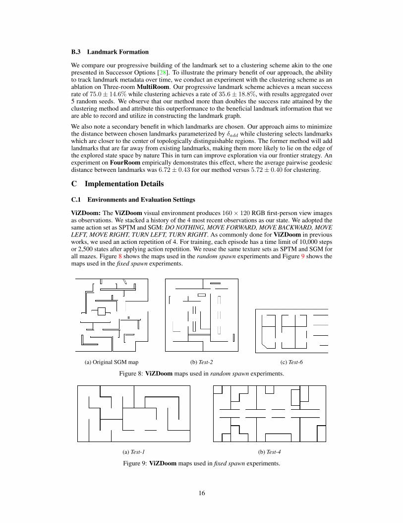
ViZDoom: The ViZDoom visual environment produces 160× 120 RGB first-person view imagesas observations. We stacked a history of the 4 most recent observations as our state. We adopted thesame action set as SPTM and SGM: DO NOTHING, MOVE FORWARD, MOVE BACKWARD, MOVELEFT, MOVE RIGHT, TURN LEFT, TURN RIGHT. As commonly done for ViZDoom in previousworks, we used an action repetition of 4. For training, each episode has a time limit of 10,000 stepsor 2,500 states after applying action repetition. We reuse the same texture sets as SPTM and SGM forall mazes. Figure 8 shows the maps used in the random spawn experiments and Figure 9 shows themaps used in the fixed spawn experiments.

(a) Original SGM map (b) Test-2 (c) Test-6

Figure 8: ViZDoom maps used in random spawn experiments.

(a) Test-1 (b) Test-4

Figure 9: ViZDoom maps used in fixed spawn experiments.

16

(a) FourRoom (b) Two-roomMultiRoom

(c) Three-roomMultiRoom

(d) Four-roomMultiRoom

Figure 10: MiniGrid maps used in fixed spawn. The agent spawns at red arrow and attempts to reachthe goal depicted by the green box.

During evaluation, the goal state is given as a first-person image observation at the goal position,stacked 4 times. For both the random spawn and fixed spawn settings, the success rate for eachdifficulty level is computed by evaluating the agent on 50 different start-goal pairs generated by eachrespective sampling procedure. The reported success rate is the success rate of reaching the goalaveraged over 5 random seeds.

MiniGrid: The MiniGrid environment provides a compact encoding of a top-down view of themaze as the state. The encoding represents each object type such as the agent or doors as a distinct3-length tuple. The state is 25 × 25 × 3 for MultiRoom and 9 × 9 × 3 for FourRoom. We usethe following action set: MOVE FORWARD, TURN LEFT, TURN RIGHT, OPEN/CLOSE DOOR.For training, each episode has a time limit of 100 steps for FourRoom and nrooms · 40 steps fornrooms-room MultiRoom, where nrooms is the number of rooms.

During evaluation, the goal state is given as the state if the agent had reached the goal. The timelimits to reach the goal are equivalent to the episode time limits during training. We compute thesuccess rate of our method and MSS over 100 trajectories each, averaging over 5 random seeds forFourRoom and 15 random seeds for MultiRoom.

C.2 Feature Learning

ViZDoom: For our experiments in ViZDoom, we adopt a similar feature learning setup as SGM byreusing the pretrained ResNet-18 backbone from SPTM as a fixed feature encoder. The networkwas originally trained with a self-supervised binary classification task: to determine whether a pairof image observations is temporally close within a time step threshold. The network encodes theimage observations as 512-length feature vectors. Recalling that our state is a stack of the 4 mostrecent observations, we use the encoder to individually embed each of the observations, and thenconcatenate the 4 intermediate feature vectors into a 2048-length feature vector.

MiniGrid: For our experiments in MiniGrid, we learn features by training a convolutional featureencoder with time-contrastive metric learning [7, 32]. Specifically, we train an encoder f via a tripletloss on 3-tuples consisting of anchor oa, positive op, and negative observations on:

||f(oa)− f(op)||22 +m < ||f(oa)− f(on)||22 (9)

A margin parameter m = 2 is used to encourage separation between the (anchor, positive) and the(anchor, negative) pairs. The 3-tuples are randomly sampled from the replay buffer such that if oacorresponds to time step t, then op is uniform randomly sampled from observations from the sameepisode with time [t−Kp, t+Kp] = [t− 2, t+ 2]. Similarly, on is randomly sampled from the timeintervals, [t− Ln, t− Un] ∪ [t+ Un, t+ Ln] = [t− 15, t− 10] ∪ [t+ 10, t+ 15].

The encoder network has the following architecture: two 3× 3 convolutional layers with 32 hiddenunits, and strides 2 and 1 respectively, each followed by ReLU activations, and ending in a linearlayer that outputs 64-dimensional feature vectors. Additionally, we normalize the feature vector suchthat ||φ(ot)||2 = α = 10 following [32]. The network is trained using the Adam optimizer [14] witha learning rate of 5e− 4 and a batch size of 128.

17

C.3 SF Learning

Recall that we estimate SF ψπ with a deep neural network parameterized by θ : ψπ(s, a) ≈ψπθ (φ(s), a). Here, φ is a feature embedding of state. The parameter θ is updated via minimizing thetemporal difference error [15, 2]:

L(s, a, s′, π, θ) = E[(φ(s) + γψ(φ(s′), π(s′))− ψπθ (φ(s), a)

)2]

(10)

where ψ is a target network that is updated at fixed intervals for stability purposes [22]. We choose forπ to be a fixed uniform random policy because we wish for the SF to capture only the structure anddynamics of the environment and not be biased towards any agent behavior induced by a particularpolicy. Consequently, we only use transitions from the random policy π for training ψπ .

We approximate the SF using a fully-connected neural network, which takes in the features (Ap-pendix C.2) as input. Each hidden layer of the network is followed by a batch normalization andReLU activation layer. For updating the parameters of the SF network, we use Adam to optimizeon the TD error loss function shown in Eq. (10) with bootstrapped n−step transition tuples. Theseexperience tuples are sampled from a replay buffer of size 100K, which stores trajectories gener-ated by 8 samplers simultaneously running SFL. For stability, we use a target network ψ that isupdated at slower intervals and perform gradient clipping as described in [22]. Table 5 describes thehyperparameters used for SF learning in each environment.

ViZDoom MiniGridHyperparameter

Hidden layer units 2048, 1024 512Learning rate 1e− 4 5e− 4

Batch size 128 128n−step 5 1

Replay buffer size 100K 20KDiscount γ 0.95 0.99

ψ update interval 1000 250Gradient clip δ 5 1

Table 5: Hyperparameters used in SFL for learning SF for each environment.

ViZDoom MiniGridHyperparameter

δadd 0.8 0.99δlocal 0.9 1δedge - 1Nfront 1000 40Nexplore 500 40εtrain 0.05 0.1εeval 0.05 0.05

Table 6: Hyperparameters used in SFL’s landmark graph, planner, and navigation policy for eachenvironment. See Appendix D.2 for details of δedge in ViZDoom.

Because the cardinality of MiniGrid’s state space is much smaller, we restrict SFL to have at most10 landmarks for FourRoom and 30 landmarks for MultiRoom, which is consistent with the numberof landmarks used in MSS as described in Table 8.

C.4 SFL Hyperparameters

We mainly tuned these hyperparameters: learning rate, δadd, and δlocal. In ViZDoom forexample, we performed grid search over the values of [10−3, 10−4, 10−5] for learning rate,[0.70, 0.75, 0.80, 0.85, 0.90] for δadd, and [0.70, 0.80, 0.9, 0.950] for δlocal on the Train map.

18

The best performing values were then used for all other ViZDoom experiments. We found that ourmethod performed well under a range of values for δadd, and δlocal. In Table 7, we report the successrates achieved on Hard tasks from a seed-controlled experiment on the Train map for random spawn.

δadd Success Rate

0.70 41%0.80 46%0.90 47%

δlocal

0.80 24%0.90 46%0.95 44%

SGM [16] 26%

Table 7: The success rates on Hard tasks in Train ViZDoom map for random spawn for varyingvalues of δadd and δlocal. For reference, SGM is included as the best-performing baseline.

The other hyperparameters were either chosen from related work or not searched over.

C.5 Optimizations

We perform optimizations on certain parts of SFL for computational efficiency. To add landmarks, wefirst store states which pass the SFS add threshold, SFS < δadd, to a candidate buffer. Then, Ncandlandmarks are added from the buffer every Nadd steps. Additionally, we update the SF representationof the landmarks every Nupdate steps and form edges in the landmark graph every Nform−edgessteps. Finally, we restrict the step-limit for reaching a frontier landmark to be nland times the numberof landmarks on the initially generated path so that we do not overly allocate steps for reachingnearby landmarks.

In ViZDoom, Ncand = 50, Nadd = 20K, Nupdate = 10K, Nform−edges = 20K, nland = 30.In MiniGrid, Ncand = 1, Nadd = 3K, Nupdate = 1K, Nform−edges = 1K, nland = 8.

C.6 Mapping State Space Implementation

We slightly modify the Mapping State Space (MSS) method to work for our environments.

ViZDoom: Similar to SGM’s and our setup, we reuse the pretrained ResNet-18 network from SPTMas a fixed feature encoder f . The UVFA embeds the start and goal states as feature vectors with thisencoder, concatenates them into a 4096-length feature vector, and it them through two hidden layersof size 2048 and 1024, each followed by batch normalization and ReLU activation. The outputs arethe Q-values of each possible action. The UVFA is trained with HER, which requires a goal-reachingreward function. Because states in ViZDoom do not directly give the agent’s position, we define thereward function based on the cosine similarity between feature vectors given with f :

rt = R(st, at, g) =

{0 f(s

′

t) · f(g) > δreach−1 otherwise

(11)

In the function above, we normalize the feature vectors such that ||f(·)||2 = 1 and set δreach = 0.8.

Landmarks are chosen according to farthest point sampling performed in the feature space imposedby the encoder f . During training, the planner randomly chooses a landmark as a goal and attemptsto navigate to that goal for 500 steps. The agent then uses an epsilon greedy policy with respect tothe Q-values given by the UVFA for a randomly sampled state as the goal for 500 steps. It cyclesbetween these two phases until the episode is over.

19

ViZDoom FourRoom MultiRoomHyperparameter

Learning rate 10−4 10−4 10−3

Batch size 128 256 128Replay buffer size 100K 100K 100K

Discount γ 0.95 0.99 0.99Target update interval 100 50 50

Clip threshold -25 -3 -5Max landmarks 250 10 30

HER future step limit 400 10 20Planner εplan - 0.75 0.75

Explore εexplore 0.25 0.10 0.10Evaluation εeval 0.05 0.10 0.05

Table 8: MSS hyperparameters used for each environment.

MiniGrid: The UVFA in MiniGrid directly maps observations to action q-values. The UVFAis composed of an encoder with the same architecture as in Appendix C.2 and a fully-connectednetwork with one hidden layer of size 512 followed by a ReLU activation. Like in ViZDoom, theUVFA encodes the start and goal states, concatenates the feature vectors together, and passes theoutput through the fully-connected network. For HER, we reuse the MSS reward function, settingδreach = 1, i.e. a reward is given only when the agent’s next state is the actual goal state. Duringtraining, at every time step, the agent will use the planner with epsilon εplan. Otherwise, it will usethe epsilon greedy policy like in ViZDoom above.

Table 8 describes the hyperparameters we used for each environment, which were determined afterrounds of hyperparameter tuning. We give extra attention to the clip threshold and max landmarksparameters, which MSS [11] mentions are the main hyperparameters of their method.

C.7 EC-augmented SPTM/SGM Implementation

We use Episodic Curiosity (EC) [30] as an exploration mechanism to enable SPTM and SGM towork in the fixed spawn setting on ViZDoom. Specifically, we leverage the exploration abilities ofEC to generate trajectories that provide greater coverage of the state space. SPTM and SGM thensample from these trajectories to populate their memory graphs and to train their reachability andlow-level controller networks. Fortunately, the code repository4 for EC already has a ViZDoomimplementation, so minimal changes were required to make it compatible with our experimentalsetting.

The full procedure is as follows. First, we train EC on the desired evaluation maze and recordthe trajectories experienced. Second, we take a frozen checkpoint of the EC module and use it togenerate trajectories for populating the memory graphs. Third, we train the SPTM/SGM networkson EC’s training trajectories recorded in the first step. Last, we run SPTM/SGM as normal with theconstructed memory graph and trained networks.

To make the comparison fair with our method and MSS, we load in the weights from the pretrainedResNet-18 reachability network from SPTM as initial weights for EC’s reachability network. In thefirst step, we train EC for 2M environment steps, which is the same number of steps we allow forour method to train. Similar to the random spawn experimental setup, we also use the pretrainedSPTM/SGM reachability and low-level controller networks, and fine-tune them in the third step with4M steps of training data from the EC-generated trajectories.

We run validation experiments with EC on the original SGM map to search over the followinghyperparameters: curiosity bonus scale α, EC memory size, and EC novelty threshold. We leveragean oracle exploration bonus based on ground-truth agent coordinates as the validation metric. Thesame oracle validation metric is used to determine which frozen checkpoint to use in the second step,generating exploration trajectories to populate the memory graph. For the other hyperparameters,we reuse the values chosen for ViZDoom in the original EC paper [30]. Table 9 describes thehyperparameters that we selected for EC.

4https://github.com/google-research/episodic-curiosity

20

Hyperparameter Value

Learning rate 2.5× 10−4

PPO entropy coefficient 0.01Curiosity bonus scale α 0.030

EC memory size 400EC reward shift β 0.5

EC novelty threshold bnovelty 0.1EC aggregation function F percentile-90

Table 9: EC hyperparameters used to generate exploration trajectories for SPTM and SGM.

C.8 Computational Resources

Each SFL run uses a single GPU and we use 4 GPUs in total to run the SFL experiments: 2 NVIDIAGeForce GTX 1080 and and 2 NVIDIA Tesla K40c. The code was run on a 24-core Intel Xeon CPU@ 2.40 GHz.

C.9 Asset Licenses

Here is a list of licenses for the assets we use:

1. rlpyt code repo: MIT license

2. ViZDoom environment: MIT license

3. MiniGrid environment: Apache 2.0 license

4. MSS code repo: MIT license

5. SPTM code repo: MIT license

6. SGM code repo: Apache 2.0 license

7. EC code repo: Apache 2.0 license

D Tackling Perceptual Aliasing in ViZDoomPerceptual aliasing is a common problem in visual environments like ViZDoom, where two imageobservations look visually similar, but correspond to distant regions of the environment. This problemcan cause our agent to erroneously localize itself to distant landmarks, which in turn harms theaccuracy of the landmark graph and planner. Figure 11 gives examples of the perceptual aliasingproblem where the pairs of visually similar observations also have very high SFS values relative toeach other. We take several steps to make SFL more robust to perceptual aliasing, as described in thefollowing sections.

Figure 11: Examples of perceptual aliasing in ViZDoom. Same colored dots correspond to pairs ofperceptually aliased observations which have pairwise SFS values > δlocal = 0.9.

21

D.1 Aggregating SFS over Time

We adopt a similar procedure used in SGM and SPTM [16, 29] to make localization more robust byaggregating SFS over a short temporal window. Specifically, we maintain a history of SFS valuesover the past W steps, and output the median as the final SFS value S. This is defined as follows:

S = median([SFSπ(st−W , ·), ...,SFSπ(st, ·)]) (12)

where SFSπ(st, ·) is the |L|-length vector containing SFSπ(st, l),∀l ∈ L. The median function istaken over the time dimension such that S is length |L|. Then, for example, if we were attempting toadd st as a landmark, we would compute lt = argmaxl∈L Sl and check if Slt < δadd to decide if weshould add st as a landmark. For our experiments, we set W = 8.

D.2 Edge Threshold

We give special consideration to the edge threshold δedge in ViZDoom due to the larger scale ofthe environment and recognized that a fixed edge threshold may not work depending on the stageof training. For example, a low value of δedge would allow connections to form in the early stagesof training, but would also introduce unwanted noise to the graph as the number of nodes grows.Therefore, we wish for δedge to dynamically change depending on the status of the graph. We defineit as follows:

δedge = medianli→lj

(N lli→lj ) (13)

In other words, an edge is formed if the number of landmark transitions on that edge is greater thanthe median number of landmark transitions from all edges. We found that the median is a suitablethreshold for enabling sufficient graph connectivity in the beginning while also reducing the thenumber of erroneous edges as the graph grows in scale.

D.3 Edge Filtering

We apply edge filtering to the landmark graph to reduce the number of potential erroneous edges.In random spawn experiments, we adopt SGM’s k-nearest edge filtering where for each vertex, weonly keep edges that have the top k = 5 number of transitions from that vertex. In fixed spawnexperiments, we instead introduce temporal filtering where we only keep edges between landmarksthat were added during similar time periods. Specifically, assuming landmarks are labeled by theorder in which they are added, uv ∈ G → |u − v| < τtemporal · |L|, where L is the number oflandmarks. Our intuition for temporal filtering is based on how the agent in the fixed spawn settingwill add new landmarks further and further away from the starting point as it explores more of theenvironment over time. Because the agent must pass by the most recently added landmarks at theedge of the already explored areas in order to add new landmarks, landmarks added within similartime periods are overall likely to be closer together. In our experiments, we set τtemporal = 0.1.

Additionally, we adopt the cleanup step proposed in SGM by pruning failure edges. If the agent isunable to traverse an edge with the navigation policy, we remove that edge. To account for the casewhere the edge is correct, but the goal-conditioned policy has not yet learned how to traverse thatedge, we "forget" about failures over time such that only edges that are repeatedly untraversable areexcluded from the graph. The agent forgets about failures that occurred over 80K steps ago.

These procedures can improve the quality of the landmark graph. Figure 12 shows the landmarkgraph formed in one of our ViZDoom fixed spawn experiments when no additional edge filteringsteps are used. The graph has many incorrect edges which connect distant landmarks. On theother hand, Figure 13 shows the landmark graph with temporal filtering and failure edge cleanup.These procedures eliminate many of the incorrect edges, resulting in a graph which respects the wallstructure of the maze to a much higher degree.

E SFL Analysis

We conduct further analysis on the components of SFL to study how each contributes to the agent’sexploration, goal-reaching, and long-horizon planning abilities.

22

Figure 12: Graph formed with only empirical landmark transitions: |L| = 517, |E| = 8316.

Figure 13: Graph formed with empirical landmark transitions, temporal filtering, and failure edgecleanup: |L| = 517, |E| = 2984.

E.1 Exploration

For our fixed spawn experiments, as the agent progresses in training, it should spend more timein faraway areas of the state space. In Figure 14a, we show that our agent exhibits this behavior.Each landmark is colored by the relative rank of its visitations, where a lighter color corresponds tospending more time at a landmark. Early in training (top), the agent has discovered some farawaylandmarks, but does not spent much time in these distant areas as indicated by the darker color ofthese landmarks. Later in training (bottom), the agent has both added more landmarks and spent moretime near distant landmarks. This is also shown by how the lighter colors are more evenly distributedacross the map. We expect agents without effective exploration strategies to remain near the center ofthe map.

E.2 Goal-Conditioned Policy

We study how the goal-conditioned policy improves over training. Figure 14b shows how the goal-conditioned policy’s success rate over certain landmark edges increases over time, with success

23

(a) (b)Figure 14: Visualizations of exploration (left) and goal-conditioned policy (right) on the fixed spawnTest-1 ViZDoom maze. Left: Each landmark colored according to the relative rank of its visitationsat different time steps. Right: Landmark edges colored by goal-conditioned policy success rate atdifferent time steps. Only edges with ≥ 80% success rate are shown.

defined as reaching the next landmark within 15 steps. On top, we see that the policy is only accuratefor edges near the start position during an early stage of training. Additionally, there is an incorrect,extra long edge that is most likely attributed to localization errors that will be corrected later on asthe agent further trains its SF representation. On the bottom, we observe that the goal-conditionedpolicy improves in more remote areas after the agent has explored more of the maze and completedmore training.

E.3 Planning with Landmark Graph

Here, we look at the long-horizon landmark paths that the SFL agent plans over the graph. Examplesof planned paths are shown in Figure 15. We observe that the plans accurately conform to the maze’swall structure. Additionally, consecutive landmarks in the plan are not too far apart, which helpsthe success rate of the goal-conditioned policy because SFS is more accurate when the start-goalstates are within a local neighborhood of each other. We acknowledge that the planned paths can belonger and more ragged than the optimal shortest path to the goal. The partial observability of theenvironment is one primary reason for this, where there are multiple first-person viewpoints per (x, y)location. For example, two landmarks may be relatively closer in terms of number of transitions evenif they appear further away on the top-down map because they both share a 30◦ view orientation.

F Mapping State Space Analysis

In this section, we offer additional analysis on Mapping State Space (MSS) and elaborate on potentialreasons why the method struggles to achieve success in our environments. Our study is conducted inthe context of fixed spawn experiments in ViZDoom.

F.1 UVFA

The UVFA is central to the MSS method, acting as both an estimated distance function and a localgoal-conditioned navigation policy. First, we qualitatively evaluate how well the UVFA estimates the

24

Figure 15: Examples of planned paths for various start (pink dot) and goal (yellow square) locations.The paths are formed by conducting planning on the landmark graph. These examples are taken fromone of the fixed spawn experiments on the Test-1 map.

distance between states by creating heatmaps similar to those in Figure 6. We use a trained UVFA toestimate the pairwise distances between a reference state and a random set of sampled states, andplot those distances in Figure 16. The top row shows the distance values for all states; the bottomrow shows the distance values for states which clear the edge clip threshold = −5 and consequentlywould have edges to the reference state. We choose a edge clip threshold smaller than the one used inour experiments to reduce the number of false positives and for ease of visualization. We observethat the estimated distances are noisy overall, where many states far away from the reference state aregiven small distances which pass the edge clip threshold. These errors cause the landmark graph tohave incorrect edges that connect distant landmarks As a result, the UVFA-based navigation policycannot accurately travel between these distant pairs of landmarks.

We hypothesize that the UVFA is inaccurate because the learned feature space does not perfectlycapture the agent’s (x, y) coordinates for localization. This causes errors in the HER reward functionwhere it may give a reward in cases when the agent has not yet reached the relabeled goal state.This is exacerbated by the perceptual aliasing problem. With this noisy reward function, the UVFAlearning process becomes very challenging.

For further analysis, we re-train the UVFA with a HER reward function that is given the agent’sground-truth (x, y) coordinates. Now, the agent is only given a reward when it exactly reaches therelabeled goal state. We recreate the same UVFA-estimated distance heatmaps using this trainingsetup, shown in Figure 17.

We see in the left column that states which pass the edge clip threshold are now more concentratednear the reference state. However, the estimated distances are still very noisy, especially in the rightcolumn where the reference state is in a distant location. We believe that learning an accurate distancefunction remains difficult because the features inputted into the UVFA only give a rough estimate ofthe agent’s (x, y) position rather than capture it fully.

F.2 Landmarks

MSS uses a set of landmarks to represent the visited state space. From a random subset of states inthe replay buffer, the landmarks are selected using the farthest point sampling (FPS) algorithm, whichis intended to select landmarks existing at the boundary of the explored space. Figure 18 shows thelandmarks selected near the end of training in a MSS fixed spawn experiment. We note that when we

25

Figure 16: Distances estimated with MSS’ UVFA relative to a reference state (blue dot) in the fixedspawn ViZDoom maze. The left column uses the agent’s start state as the reference state while theright column uses a distant goal state as the reference state. The top row depicts all states while thebottom row shows states with distance >= −5, the edge clip threshold. States that do not pass thethreshold, i.e. distance < −5 are darkened.

Figure 17: Distances estimated with MSS’ UVFA relative to a reference state (blue dot) in the fixedspawn ViZDoom maze. We assume a similar setup as Figure 16, but the UVFA is trained using HERwith ground-truth (x, y) coordinate data.

26

Figure 18: Landmarks selected using FPS in a MSS fixed spawn experiment.

increase the max number of landmarks in our experiments, the observed performance either decreasesor remains the same.

The set of landmarks only partially covers the maze, thereby limiting the agent’s ability to reach andfurther explore distant areas. Because FPS operates in a learned feature space, the estimated distancesbetween potential landmarks can be noisy, leading to inaccurate decisions on which landmarks shouldbe chosen. Furthermore, MSS does not explicitly encourage the agent to navigate to less visitedlandmarks. States in unexplored areas become underrepresented in the replay buffer and therefore,are unlikely to be included in the initial random subset of states from which landmarks are chosen.

G Episodic Curiosity Analysis

In this section, we conduct additional experiments regarding the Episodic Curiosity (EC) augmentedSPTM and SGM baselines to better understand the benefits and shortcomings of these combinedmethods. This study is completed within the context of fixed spawn experiments in ViZDoom.

We run ablations of the EC + SPTM and EC + SGM baselines on the Test-1 map within the fixedspawn evaluation setting. Two components of SPTM/SGM are changed in the ablations: the high-level graph, and the reachability and locomotion networks. Specifically, we vary how we collect thetrajectories used to populate the graph and to train the two networks. The trajectories are generatedby the following agent variations:

1. Fixed start (FS): randomly acting agent that begins each episode in the same starting location.2. Random start (RS): randomly acting agent that begins each episode in a starting location that is

sampled uniform randomly across the map.3. EC: agent running the EC exploration module and begins each episode in the same starting

location.

For populating the graph, the agents build and sample from a replay buffer containing trajectoriesof 100 episodes of 200 steps each, following the setup of SGM [16]. The EC agent uses a frozencheckpoint of its reachability and policy networks when collecting these trajectories. The setup fortraining the reachability and locomotion networks of SPTM/SGM remains the same except the agentused to generate the training data is varied between FS, RS, and EC. For the EC variant, the trainingdata is composed of trajectories that were recorded during the training of the exploration module.

We then evaluate the underlying baselines initially described in Section 5.2, visual controller5, SPTM,and SGM, with ablations of the methods used to populate the graph and train the networks. Wereport their success rates averaged over 5 random seeds in Table 10. The EC (populate graph) + FS(train networks) + SPTM/SGM baselines (underlined) are the ones reported in the main paper in

5The visual controller baseline does not use a high-level graph for planning.

27

Method Used Test-1Populate Graph Train Networks Evaluation Easy Medium Hard Hardest

- FS Controller 43% 12% 0% 0%- RS Controller 29% 2% 1% 0%- EC Controller 39% 6% 0% 1%

FS FS SPTM 32% 4% 0% 0%RS RS SPTM 32% 6% 0% 0%EC FS SPTM 48% 16% 2% 0%EC EC SPTM 46% 12% 4% 4%

FS FS SGM 41% 8% 0% 0%RS RS SGM 24% 1% 0% 0%EC FS SGM 43% 3% 0% 0%EC EC SGM 29% 0% 0% 0%

MSS 23% 9% 1% 1%SFL [ours] 85% 59% 62% 50%

Table 10: (Fixed spawn) The success rates of ablations of SPTM and SGM baselines on the Test-1ViZDoom map. For each difficulty level, we bold the success rate of the best-performing ablationbaseline for emphasis. We also include the success rates of MSS and our method SFL for reference.

(a) FS (b) EC (c) RS

Figure 19: State coverage of the replay buffers built by the FS, EC, and RS agents.

Table 2. From these experiments, we make the following observations. First, using EC-generatedtrajectories for populating the graph can improve SPTM’s performance on longer-horizon goals. Thisis expected as the exploration bonus from EC supports greater coverage of more distant areas ofthe state-space, which thereby enables graph planning to distant goals. Second, we find that theFS-generated trajectories, while limited in their coverage of distant areas, can outperform RS and ECon the Easy and Medium difficulties. We hypothesize that this is due to how fixed spawn start-goalpairs in evaluation share the same starting location as in training. With the FS trajectories, the trainingof the networks is skewed towards goals closer to the starting location. Conversely, RS trajectoriessuffer by having episodes start from a different location than the start location of the evaluationsetting.

We also visualize the state coverage of the replay buffers used for populating the graph for the FS, EC,and RS agents in Figure 19.6 The EC agent is able to store observations from more distant locationsin comparison to the FS agent. As expected, the RS agent provides comprehensive coverage of theentire map.

6The four distinct white squares are caused by the presence of peripheral in-game objects.

28

H Additional Details: Traverse Algorithm

Here is the Traverse algorithm used for localizing the agent to the nearest landmark (lcurr) based onSFS and traversing to the next target landmark (ltarget) on the landmark path with the goal-conditionedpolicy(πl). The procedure is repeated until either the target landmark is reached or the “done” signalis given indicating that the episode is over. This algorithm is referenced in Algorithm 1.

Algorithm 3 Traverseinput πl, ltargetoutput τtraverse, lcurr

1: τfront ← ∅2: while lcurr! = ltarget or env not done do3: (s, a, r) ∼ πl(·; ltarget)4: lcurr ← argmaxl∈L SFSπθ (s, l) {localize agent}5: τtraverse = τtraverse ∪ (s, a, r)6: end while7: return τtraverse, lcurr

I Societal Impact

Our Successor Feature Landmarks (SFL) framework is designed to simultaneously support explo-ration, goal-reaching, and long-horizon planning. We expect for our method to be applicable toreal-world scenarios where an autonomous agent is operating in a large environment and must com-plete a variety of complex tasks. Common examples include warehouse robots and delivery drones.SFL can improve the efficiency and reliability of these autonomous agents, which offer potentialbenefit to human society. However, these autonomous systems may also be built for more maliciouspurposes such as for constructing weaponry or conducting unlawful surveillance. In general, thesepotential harms should be carefully considered as we begin to develop autonomous agents and passlegislation that will govern these systems.

29