subjective performance and the value of blind evaluation

Review of Economic Studies (2010) 01, 1�37 0034-6527/10/00000001$02.00

© 2010 The Review of Economic Studies Limited

Subjective Performance and the Value of BlindEvaluation1

CURTIS R. TAYLOR

Duke University

HUSEYIN YILDIRIM

Duke University

First version received November 2008; �nal version accepted June 2010 (Eds.)

The incentive and project selection e�ects of agent anonymity are investigated in asetting where an evaluator observes a subjective signal of project quality. Although theevaluator cannot commit ex ante to an acceptance criterion, she decides up front betweeninformed review, where the agent's ability is directly observable, or blind review, where it isnot. An ideal acceptance criterion balances the goals of incentive provision and projectselection. Relative to this, informed review results in an excessively steep equilibriumacceptance policy: the standard applied to low-ability agents is too stringent and thestandard applied to high ability agents is too lenient. Blind review, in which all types facethe same standard, often provides better incentives, but it ignores valuable informationfor selecting projects. The evaluator prefers a policy of blind (resp. informed) review whenthe ability distribution puts more weight on high (resp. low) types, the agent's payo� fromacceptance is high (resp. low), or the quality signal is precise (resp. imprecise). Applicationsdiscussed include the admissibility of character evidence in criminal trials, and academicrefereeing.

�If Justice is pictured blindfold, it is because she judges causes, not men, andnot because the prime faculty of an arbitrator is lack of discernment.�

�Charles Wagner, Justice, 1905, p. 133.

1. INTRODUCTION

The settings in which an evaluator must rely only on her subjective impressions to judgeoutput or performance are ubiquitous. In cultural environments individuals are askedto evaluate wine, food, art, poetry, movies, and music. In retail settings experts andpanel participants review a vast array of consumer products. In criminal trials andlawsuits, juries are charged with weighing evidence, and in academia faculty evaluateexams, manuscripts, and grant proposals. Given that subjective evaluation is endemicto so many signi�cant situations, it is important to understand what elements add ordetract from its e�cacy. A key question in this regard is whether or not the reviewershould be permitted to use supplemental information such as the applicant's identity andprior record in the current evaluation, i.e., should the reviewer be �informed� or �blind�?

1. The authors thank Andrea Prat, four anonymous referees, and numerous seminar participantsfor helpful comments. They also bene�ted from suggestions by Atila Abdulkadiro§lu, Peter Arcidiacono,Jeremy Burke, Yeon-Koo Che, Andrew Daughety, Preston McAfee, Marco Ottaviani, and JenniferReinganum. Sergiu Ungureanu provided valuable research assistance. The authors are responsible forany remaining errors.

1

2 REVIEW OF ECONOMIC STUDIES

At �rst glance, the answer to this question may seem obvious: in situations wherean individual's current output or performance � and not his innate ability � is the objectof evaluation, the review process should be blind whenever feasible in order to minimizebias.1 Note, however, that not all �bias� is undesirable. Because evaluation is often noisy,an e�ective use of information may dictate that individuals with stronger track recordsface lower standards.

In fact, the mode of review, blind or informed, varies both across and withinevaluation settings. Wine tasting, for example, is virtually always performed blindly.2 Similarly, in classical music, Goldin and Rouse (2000) note that most major U.S.symphony orchestras adopted some form of blind auditioning for hiring new members inthe 1970s and 80s. Likewise, nearly all licensing and competency examinations such asbar exams and medical board exams are scored blindly.3

There are numerous settings in which a mixture of blind and informed reviewprocedures are employed. For instance, there is a long-standing controversy amonglegal scholars about when judges should allow juries to hear character evidence, whatMcCormick (1954, pp. 340�41) de�nes as �a generalized description of one's disposition,or of one's disposition in respect to a general trait such as honesty, temperance, orpeacefulness.� Prior to the advent of Internet search engines, there was a similar debatein academia about whether journal submissions should be reviewed blindly. Blank (1991)reports that among 38 well-known journals in chemistry, biology, physics, mathematics,history, psychology, political science, sociology, and anthropology, 11 used blind review,as did 16 of 38 major economics journals. In a more recent survey of 553 journals across18 disciplines, Bachand and Sawallis (2003) �nd that 58% employed blind review.

There are also numerous settings in which informed review is the predominant modeof evaluation. For example, the identity of students is commonly known to the graderwhen evaluating course examinations and projects. Similarly, grant proposals typicallycontain not only a description of the project, but the academic track record of the primaryinvestigator; i.e., his education, major publications, and previous grants.

Most extant studies on the e�ects of blind versus informed review (summarized in thenext section) have been experimental or empirical. While revealing important insights,many of these investigations have presented con�icting evidence, making it di�cult � inthe absence of a coherent theory � to draw general conclusions or make consistent policyrecommendations. In this paper we study a simple game-theoretic model that focuseson three common features of many review processes: (1) the applicant can improve thequality of his project by expending e�ort; (2) evaluation is a noisy process in which thereviewer observes only an imperfect subjective signal of quality; and (3) knowing theidentity of the applicant would provide the reviewer with additional information abouthis ability to produce a high quality project.4

1. Of course, one reason to adopt blind review is to avoid taste-based discrimination such asracism or sexism (or charges thereof) by evaluators. While this is clearly an important consideration inmany settings, the model presented here focuses on a type of statistical discrimination (Arrow, 1973) inwhich blind review forces an evaluator to ignore an agent's productivity.

2. See Taber (2005) for an account of the most famous blind tasting, the Judgment of Paris, heldin 1976, which is accredited with putting California wines on the world stage.

3. Bar exams in the U.S. contain an essay section which involves subjectivity in grading. Similarly,the United States Medical Licensing Exam contains a Clinical Skills section on which medical studentsand graduates are evaluated according to several subjectively scored criteria.

4. Ottaviani and Wickelgren (2009) also investigate an evaluation setting but with quite di�erentfeatures; e.g., symmetric information and learning.

TAYLOR & YILDIRIM SUBJECTIVE PERFORMANCE 3

The applicant cares only about having his project accepted, while the evaluator is aBayesian decision maker who weighs her payo�s from accepting good and bad projects.5

The equilibrium of the model is examined under three regimes: commitment � which isan ideal benchmark setting where the quality signal is veri�able and the evaluator cancredibly commit up front to an acceptance criterion, informed review � in which theevaluator observes the applicant's ability, and blind review � in which the applicant'sability is hidden. In all three cases the reviewer follows a simple equilibrium strategy:accept the project if and only if the quality signal is above a certain threshold, or standard.

Under informed review, the evaluator � not surprisingly � applies weak standards tohigh-ability applicants and tough standards to low-ability ones. In fact, these standardsare too weak and too tough when compared with the ideal review process. In a sense,the benchmark process calls for a more �fair� standard across applicants, even though nodirect preference for equity is assumed.

The reason the ideal review policy is �atter than the one implemented underinformed review is that it is designed not only to select good projects, but also to provideincentives to produce them. Both weak and tough standards generate poor incentives,albeit for opposing reasons. The marginal return to e�ort is low to an agent who iseither very likely to have his project accepted or very likely to have it rejected. Theoptimally designed acceptance policy thus creates better incentives for agents at bothends of the type distribution by raising the standards facing high-ability agents andlowering those facing low-ability ones. This policy, however, is not time-consistent. Oncethe applicant has invested e�ort in the project and submitted it for evaluation, thereviewer would prefer to renege and apply a steeper (informationally-e�cient) acceptancepolicy. Hence, if the quality signal observed by the evaluator is not veri�able (e.g., becauseit is impossible or impractical to quantify), then it will not be possible for her to crediblyimplement the relatively �at ideal acceptance criterion. It may, however, be possible forher to commit to remain ignorant about the applicant's type and apply a completely �atstandard; that is, to perform blind review.

Under blind review, the evaluator sets a uniform standard as if she were assessing anapplicant of average ability. This policy provides good incentives for applicants at bothends of the type distribution, but blind review is also clearly suboptimal when comparedwith the ideal policy. Speci�cally, blind review does not allow the evaluator to use anyinformation about applicant ability to mitigate noise in the review process.

Hence, both informed and blind review procedures are suboptimal, but for di�erentreasons. On one hand, ex post project selection is better under informed review, on theother hand, ex ante incentives are often better under blind review. Thus, the evaluator'spreference between review procedures will depend on the environment, especially onthe distribution of ability in the applicant pool and the informational content of thequality signal. When the distribution of applicants contains a large proportion of high-ability agents, then assessing project quality is relatively less important than providingincentives, and the evaluator, therefore, prefers blind review. Conversely, when theapplicant pool contains a large proportion of low-ability agents, then project selectionis paramount and the evaluator prefers informed review. In a similar vein, when thesignal on project quality is very precise, then observing the applicant's ability provideslittle additional information and blind review is optimal. On the other hand, when the

5. The model can be altered to allow the applicant to care about project quality so long as thereis some residual incongruity between his payo�s and the evaluator's.


quality signal is very imprecise, then observing ability provides signi�cant incrementalinformation, and informed review is the preferred mode of evaluation.

The remainder of the paper is organized as follows. The relevant literature is reviewedin the next section. In Section 3 the basic model is presented. Sections 4, 5, and 6 containthe analysis of the commitment benchmark, informed review, and blind review settingsrespectively. In Section 7 the factors in�uencing the evaluators equilibrium choice ofreview policy are determined. We discuss two applications of the theory in Section 8.In subsection 8.1 we contribute to the debate on character evidence, arguing that our�ndings support its use in cases of blue-collar street crime such as robbery or assaultbut not in cases of white-collar corporate crime such as embezzlement or price �xing.In subsection 8.2 we o�er an explanation of the seemingly paradoxical claim that itis optimal to use blind review to evaluate scholarly manuscripts and informed review toassess grant proposals. In Section 9 three generalizations of the basic model are analyzed:competition among evaluators (9.1), costly false rejections (9.2), and non-productivee�ort (9.3). Section 10 contains concluding remarks and a discussion of future work. Theproofs of all propositions and lemmas are relegated to the Appendix.

2. RELATED LITERATURE

There is a large empirical and experimental literature on the impact of anonymity on theacademic publication process, ably surveyed by Snodgrass (2006). In particular, papersby Blank (1991) in economics, Horrobin (1982) in modern languages, Link (1998) inmedicine, Peters and Ceci (1982) in psychology, and Zuckerman and Merton (1971) inphysics, found compelling evidence that informed review is likely to introduce status,gender, or geographical bias in evaluation of scholarly manuscripts.

In the 1970s and 80s, concern about gender-biased hiring caused most major U.S.symphony orchestras to adopt some form of blind auditioning. Goldin and Rouse (2000)estimate that the switch to blind auditions explains up to 25 percent of the increase infemale orchestra musicians hired over the intervening years.

The theoretical literature on subjective performance evaluation is relatively small[e.g., Levin (2003) and MacLeod (2003)] and almost exclusively addresses contractingproblems within an agency setting. This paper considers a complementary setting inwhich transfers between the parties are not allowed and the principal can decide toremain ignorant of the agent's ability. The perverse incentive e�ect associated with betterinformation at the core of this paper is reminiscent of similar results found in careerconcern models, either in the form of reduced e�ort by the agent [e.g., Dewatripont et al.(1999), and Holmstrom (1999)], or in the form of concealing his private information [e.g.,Morris (2001), and Prat (2005)]. Unlike in our static framework, the agent in these modelscares about the principal's belief about his ability. In the same spirit, several paperssuch as Cremer (1995), Riordan (1990), and Sappington (1986) have highlighted thepotential bene�ts of committing to an imperfect monitoring technology in a contractingenvironment. In a somewhat di�erent context, Fryer and Loury (2005) also observe thatrestrictions on what information can be used for selection may have serious consequencesfor incentives. This study also contributes to the literature on discretion versus rules (e.g.,Milgrom and Roberts (1988)), which emphasizes that commitment to even an imperfectinstitution is sometimes better than no commitment at all.

The paper also belongs to a growing literature on mechanism design withouttransfers, originating with the work by Holmstrom (1977 and 1984) in the case offull commitment, and by Crawford and Sobel (1982) in the case of no commitment.


More directly related to our investigation is the paper by Seidmann (2005). Seidmannintroduces limited commitment and imperfectly veri�able messages to the Crawfordand Sobel model to demonstrate that a �right to silence� may indirectly bene�t theinnocent by inducing the guilty to remain silent. Unlike these papers that consider hiddeninformation, we explore an environment of hidden action and compare full commitment(the benchmark), no commitment (informed review), and commitment to an imperfectinstitution (blind review).

A �nal strand of related research is the literature on statistical discrimination, whichrecognizes the potential tension between fairness and e�ciency. Papers by Norman (2003)and Persico (2002) demonstrate that a more fair treatment of di�erent groups need notinterfere with a socially e�cient allocation of resources. Depending on the elasticity ofeach group's production function, to insist on a more equal treatment can also shiftequilibrium production toward a more socially e�cient level.

The paper most closely related to this one is Coate and Loury (1993). They study amodel in which two identi�able groups that are ex ante identical invest in human capital.Employers receive noisy subjective signals regarding investment levels and decide whoto hire. There are assumed to be multiple equilibria of the investment/evaluation game.Coate and Loury suppose that one group coordinates with employers on an equilibriumwith a modest standard and higher investment, while the other group gets stuck ina Pareto inferior equilibrium with a high standard and low investment. In the settinginvestigated here, by contrast, agent ability is drawn from a continuum and representsreal ex ante heterogeneity in productivity. Moreover, players are assumed to coordinateon the unique Pareto superior equilibrium. Coate and Loury argue that forcing employersto use the same standard across groups can correct ine�cient coordination failure. Thefocus here is on a di�erent but complementary question � when is it in the best interestof an evaluator to commit herself not to use fundamentally valuable information in thereview process? The potential bene�t of blind review in this context is not to breakcoordination failure, but to raise productivity at both ends of the ability spectrum bypooling incentives.

3. THE BASIC MODEL

There are two risk-neutral parties: an applicant (the agent) and an evaluator (theprincipal) who play a three-stage game. In the �rst stage, the principal commits to areview policy, which is either informed (she directly observes the agent's type) or blind(she does not observe the agent's type).

In the second stage, the agent, who knows the review policy and knows his own typeθ, exerts e�ort p ∈ [0, 1] to prepare a project for review by the principal. The ultimatequality of the project is high (q = h) with probability p, or low (q = l) with probability1− p.6 The agent's e�ort cost is given by

C(p; θ) =p2

2θ,

6. The focus of this investigation is the tradeo� between provision of incentives and the e�cientuse of information. Although there are a number of ways of exploring this tradeo�, the setting consideredhere is probably the simplest. A version of the model with continuous quality yields similar results; seeTaylor and Yildirim (2007).


where θ ∈ [θ, θ] ⊂ R+.7 Hence, θ is a measure of the agent's productivity and may

represent either his innate ability or his experience.In the �nal stage of the game the agent submits the project to the principal for

evaluation. The principal does not observe p or q directly, but receives a subjective (i.e.,non-veri�able) signal of quality, σ ∈ [σ, σ]. Based upon the outcome of this signal � andthe agent's type if the review policy is informed � the principal decides whether to acceptor reject the project.

The principal prefers to accept high-quality projects and to reject low-quality ones.In particular, her exogenous payo� from accepting a high-quality project is v > 0 andfrom accepting a low-quality one is −c < 0. Her payo� from rejecting a low-qualityproject is taken to be zero, which is sensible since she otherwise could get �somethingfor nothing� in a degenerate equilibrium where she always rejects and the agent neverexerts e�ort. The principal's cost from rejecting a high-quality project is also taken to bezero. This greatly simpli�es the analysis and is reasonable in many settings. The moregeneral case in which she also su�ers a loss from a false rejection is, however, analyzedin subsection 9.2. It is notationally convenient to de�ne the principal's cost bene�t ratiofrom accepting a project by r ≡ c

v .The agent prefers the project to be accepted, regardless of its underlying quality.

Speci�cally, he receives an exogenous gross payo� of u > 0 if the principal acceptsthe project, and zero if she rejects it. No monetary transfers between the parties arepermitted.

The agent's type, θ, is distributed according to the distribution function G(·),possessing density g(·) and �nite mean E[θ]. The signal, σ, is drawn from one oftwo distributions: Fh(·) (with density fh(·)) if project quality is high, or Fl(·) (withdensity fl(·)) if it is low. For analytical convenience, assume fq(·) is bounded and twice

di�erentiable. The likelihood ratio is de�ned by L(σ) ≡ fh(σ)fl(σ)

, and satis�es the following

regularity conditions.

Assumption 1 (Signal Technology). The Likelihood ratio satis�es:

(i) L′(σ) > 0,

(ii) L(σ) = 0 and L(σ) =∞,

(iii) limσ→σ L(σ)(1− Fq(σ)) = λq exists for q ∈ {l, h} and λh > 0.

Part (i) is the familiar monotone likelihood ratio property (MLRP) indicating thathigher signals are associated with high project quality. Part (ii) says that the mostextreme signals (which occur with probability zero) are perfectly informative. Thisensures equilibrium existence. Part (iii) is a boundary condition used below to identifythe set of agent types that exert zero e�ort in equilibrium. The requirement λh > 0 isnecessary because all types of agent would otherwise exert zero e�ort under informedreview. All aspects of the environment are common knowledge, and the solution conceptis Pareto e�cient Perfect Bayesian equilibrium (PBE).

Example 1 (Signals). The following signal technology will be used in illustrativeexamples below. The principal's subjective signal, σ, is drawn from one of the two

7. The functional form assumed for the e�ort cost is analytically helpful but not critical for thequalitative nature of the results presented below.


triangular densities on [0,1]: fh(σ) = 2σ or fl(σ) = 2(1− σ). This implies L(σ) = σ1−σ ,

λh = 2, and λl = 0 in agreement with Assumption 1.

4. THE COMMITMENT BENCHMARK

The fundamental problem facing the principal is an inability to commit. Because herevaluation results in a non-veri�able assessment, once the principal observes σ, she willaccept the project if an only if she expects a positive payo�. While this is optimalex post (after the agent has sunk e�ort), it is not generally desirable from an ex anteperspective. To highlight this, the benchmark case of the principal's optimal review policywith commitment is characterized in this section.

To begin, note that there is no scope for blind review in this context. With fullpower of commitment, the principal can choose to ignore information whenever it isadvantageous. Next, it is straightforward to verify that MLRP implies the principaloptimally uses a standard s(θ) when conducting a review. That is, she accepts the projectof a type θ agent if and only if σ ≥ s(θ).

Given an arbitrary standard s, a type θ agent will choose p so as to maximize hisexpected payo�

U(p, s; θ) = u[p(1− Fh(s)) + (1− p)(1− Fl(s))]−p2

2θ, (4.1)

subject to the downward and upward feasibility restrictions, p ≥ 0 and p ≤ 1. The �rstterm in (4.1) is the agent's bene�t from acceptance u times the probability the projectis accepted whether it is good p(1 − Fh(s)) or bad (1 − p)(1 − Fl(s)), while the secondterm is his cost of e�ort, C(p, θ).

Combining the �rst-order condition with the upward feasibility restriction yields theagent's reaction function:

P (s, θ) = min{θu(Fl(s)− Fh(s)), 1}. (4.2)

If the feasibility restriction does not bind, then the agent's reaction function is�hump-shaped� in s. To see this, note �rst that the most extreme standards elicit noe�ort at all, P (σ, θ) = P (σ, θ) = 0. Next, de�ne the neutral signal by s∗ ≡ L−1(1). Then

Ps(s, θ) = θu(1− L(s))fl(s)

is positive for s < s∗ (e�ort is increasing in the standard), and negative for s > s∗

(e�ort is decreasing in the standard). Low standards elicit little e�ort because projectsare rarely rejected and high standards elicit little e�ort because they are rarely accepted.The agent exerts maximal e�ort when facing the intermediate standard s∗. Intuitively,if σ = s∗, then the posterior on project quality is the same as the prior. Setting theneutral standard, thus, minimizes bias in the evaluation process which maximizes theagent's incentives. (See Figure 1.) If θ is su�ciently high, however, then the upwardfeasibility restriction will bind and the agent will exert e�ort of P (s, θ) = 1 over anintermediate range of standards containing s∗; i.e., the �hump� of the reaction functionwill be truncated to a �plateau.�

Inducing the agent to exert e�ort is only part of the principal's objective. An optimalreview policy must both provide incentives for the agent and select high-quality projectsas often as possible. Speci�cally, the principal will commit herself to a standard that


maximizes her expected payo�8

V (s, p) = vp(1− Fh(s))− c(1− p)(1− Fl(s)), (4.3)

subject to the agent's reaction function in (4.2).The �rst term in the principal's objective is her bene�t from accepting a good

project, v, times the probability the project is good and the standard is achieved,p(1 − Fh(s)), and the second term is her cost from accepting a bad project, −c, timesthe probability the project is bad and the standard is achieved, (1− p)(1− Fl(s)).

Substituting the agent's reaction function into (4.3) results in the function

V (s, P (s, θ)) = vP (s, θ)(1− Fh(s))− c(1− P (s, θ))(1− Fl(s)). (4.4)

This function is continuous, and hence achieves a maximum on the compact interval[σ, σ]. The following assumption ensures su�ciency of the �rst-order condition.9

Assumption 2 (Single-Peaked Preferences). The function V (s, P (s, θ)) isstrictly quasi-concave in s whenever P (s, θ) < 1.

Ignoring the feasibility restrictions for the moment and di�erentiating (4.4) withrespect to s yields the �rst-order condition

Vs(s, P (s, θ))︸︷︷︸Selection E�ect

+ Vp(s, P (s, θ))Ps(s, θ)︸︷︷︸Incentive E�ect

= 0. (4.5)

Denote the solution to this equation by sC0 (θ). This is the optimal standard theprincipal would announce for an agent whose type θ fell in the range [θC−, θ

C+ ], where the

feasibility restrictions do not bind.Equation (4.5) highlights the tradeo� facing the principal: selection versus incentives.

The �rst term in (4.5) represents the selection e�ect. As discussed in the next section,setting this term alone equal to zero results in the standard, sI(θ), that accepts a projectif and only if it has positive expected value to the principal. The second term in (4.5)represents the incentive e�ect. As discussed above, setting this term alone equal to zeroresults in the neutral standard, s∗, that maximizes the agent's e�ort. In general, it isnot possible to set both terms to zero simultaneously. In other words, there is tensionbetween the e�cient use of information and motivating the agent.

De�ne the endpoints of the interval [θC−, θC+ ] by

θC− ≡r

u(2λh + (r − 1)λl), (4.6)

and

θC+ ≡ min{θ |P (sC0 (θ), θ) = 1}. (4.7)

8. There are two situations to consider. The principal might announce the review policy eitherbefore or after observing the agent's type. Because the expectation over θ of V (s, P (s, θ)) is separablein θ, the optimal review policy in either case is found by maximizing this function with respect to s foreach value of θ ∈ [θ, θ].

9. It is easy to verify that if L(s) ≤ 1, Assumption 2 is automatically satis�ed; and if L(s) > 1, itis satis�ed whenever

−(L(s) + r−1

2)(1− Fl(s))L′(s)

(L(s)− 1)(L(s) + r)+ fl(s) < 0.

This inequality turns out not to be too stringent, owing to the assumptions that fl(s) is bounded, andlims→σ [L(s)(1− Fl(s))] exists.


The following result characterizes the benchmark solution.

Proposition 1 (Equilibrium under Commitment).

Principal: The principal sets the standard

sC(θ) ≡

σ, if θ < θC−sC0 (θ), if θ ∈ [θC−, θ

C+ ]

min{s |P (s, θ) = 1}, if θ > θC+

Moreover, sC(θ) is strictly decreasing for θ > θC−, and limθ→∞ sC(θ) = σ.Agent: The agent chooses e�ort level

pC(θ) ≡

0, if θ < θC−P (sC0 (θ), θ), if θ ∈ [θC−, θ

C+ ]

1, if θ > θC+.

Moreover, pC(θ) is continuous, and strictly increasing for θ ∈ (θC−, θC+).

The selection e�ect results in a negative relationship between an agent's ability andthe standard set for him. Higher ability agents are more likely to produce good projects,so the principal accordingly lowers the standard confronting them. This response is,however, attenuated by the incentive e�ect. In order to elicit more e�ort, the principalcommits to a pro�le of standards, sC(θ), that is �too �at� to be ex post optimal. In otherwords, under sC(θ) the principal may be forced to reject the project of a high abilityagent or accept the project of a low ability one when she would prefer to do otherwise.This is most starkly illustrated for ability levels θ ≥ θC+ . For these high-ability types,the upward feasibility restriction binds (pC(θ) = 1). Nevertheless, the standard facingsuch an agent, sC(θ), is greater than the minimum standard, σ. Hence, even though theprincipal knows for sure that the project is good, she commits herself to reject it withpositive probability. Only by doing so can she induce the agent to exert e�ort in the �rstplace.

At the other end of the spectrum are the low ability agents with θ ≤ θC−. Thesetypes of agents are e�ectively pre-screened in the sense that the principal commits neverto accept their projects; i.e., sC(θ) = σ. Consequently, these types exert no e�ort, so thedownward feasibility restriction binds (pC(θ) = 0).

Finally, it is straightforward to verify that s∗ ∈ (sC(θC+), σ). So, there exists a uniquecritical type

θ∗ ≡ r

(1 + r)u(Fl(s∗)− Fh(s∗))(4.8)

such that sC(θ∗) = s∗. For this one type of agent there is no con�ict between selectionand incentives. In particular, the standard, s∗, set for type θ∗ both induces maximale�ort and leads to an ex post optimal acceptance decision. For all other types, θ 6= θ∗,however, the benchmark solution sC(θ) strikes a balance between selecting good projectsex post and providing incentives ex ante.

Example 2 (Commitment). Suppose the signal technology of Example 1 andthat v = c = u = 1.10 From (4.2), the agent's reaction function is

P (s, θ) = min{2θs(1− s), 1}.

10. For a fully parametric example, see Taylor and Yildirim (2007).


For θ < 2 this is hump-shaped and attains a maximum at s∗ = 12 . From (4.3), the

principal's payo� is

V (s, p) = p(1− s2)− (1− p)(1− s)2.Substituting P (s, θ) into this and maximizing yields the commitment solution

sC(θ) =

1, if θ < θC−13 + 1

6θ , if θ ∈ [θC−, θC+ ](

12

) (1−

√1− 2

θ

), if θ > θC+,

where θC− = 14 and θC+ = 1 + 3

√2

4 . As Proposition 1 indicates, sC(θ) is decreasing forθ > θC−. Low types of agent with θ ≤ θC− are prescreened and induced to exert no e�ort,while high types with θ ≥ θC+ are induced to exert full e�ort. Finally, setting sC(θ) = s∗

and solving reveals that the critical type is θ∗ = 1.

5. INFORMED REVIEW

If the principal is unable to credibly commit to a standard, then she cannot act asa Stackelberg leader, maximizing her expected payo� subject to the agent's reactionfunction. (See the dashed iso-payo�s in Figure 1.) Instead, the agent's e�ort andprincipal's standard will be determined in a Cournot-Nash equilibrium.

If the principal has opted for informed review, then she observes the agent's typewhen choosing the standard. Hence, she maximizes her expected payo�, V (s, p), given in(4.3), with respect to s, holding �xed p. The �rst-order condition is

Vs(s, P (s, θ)) = −[vpL(s)− c(1− p)]fl(s) = 0. (5.9)

Rearranging this yields the principal's reaction function

S(p) = L−1(r

1− pp

). (5.10)

Note that Assumption 1 implies: S(0) = σ, S(1) = σ, and S′(p) = − rp2L′(s) < 0. This

makes sense: if the principal believes the project is certainly bad (p = 0), then no signalrealization will convince her to accept it. Similarly, if she believes the project is certainlygood (p = 1), then no signal realization will deter her from accepting it. In general, thehigher the principal believes p to be, the lower she sets the standard for acceptance.

Solving the agent and principal's reaction functions (4.2) and (5.10) results in theequilibrium standard and e�ort under informed review, (sI(θ), pI(θ)). (See Figure 1.) Adegenerate equilibrium in which the principal never accepts the project (sI(θ) = σ) andthe agent never exerts e�ort (pI(θ) = 0) always exists. Indeed, for values of θ less thana cuto� θI− this is the unique equilibrium, in which case the agent is prescreened. Forhigher values of θ, however, non-degenerate equilibria exist. In this case, the followingobservation, which obtains directly from the Envelope Theorem, implies that the set ofequilibria are Pareto rankable.

Lemma 1. (i) The principal's indirect payo�, V (S(p), p), is increasing in p.

(ii) The agent's indirect payo�, U(P (s, θ), s; θ), is decreasing in s.

Because the principal's reaction function is downward-sloping, equilibria with lowerstandards (which the agent prefers) involve higher e�ort (which the principal prefers).


Hence, when multiple equilibria exist, the one with the lowest standard and highest e�ortis Pareto superior, and the players are presumed to coordinate on it.11

Momentarily ignoring the feasibility restrictions and substituting for p in (5.9) from(4.2) gives

Vs(s, P (s, θ)) = −[vP (s, θ)L(s)− c(1− P (s, θ))]fl(s) = 0. (5.11)

De�ne sI0(θ) to be the smallest root to this equation. Then sI0(θ) is the equilibriumstandard when the feasibility restrictions on p do not bind.

De�ne the cuto� type by

θI− ≡r

u(λh − λl). (5.12)

The following result characterizes the equilibrium under informed review.

Proposition 2 (Equilibrium under Informed Review).

Principal: The principal sets the standard

sI(θ) ≡{σ, if θ < θI−sI0(θ), if θ ≥ θI−.

Moreover, sI(θ) is strictly decreasing for θ > θI− , and limθ→∞ sI(θ) = σ.Agent: The agent chooses e�ort level

pI(θ) ≡{

0, if θ < θI−P (sI0(θ), θ), if θ ≥ θI−.

Moreover, pI(θ) is strictly increasing for θ > θI−, and limθ→∞ pI(θ) = 1.

As in the commitment benchmark, higher ability agents exert more e�ort inequilibrium and therefore face lower standards under informed review. Two di�erencesfrom the commitment case are, however, readily apparent. First, at the low end of thetype space, the range over which prescreening occurs is larger under informed reviewthan under commitment (θI− > θC−). In other words, more types are induced to exertpositive e�ort under commitment. Second, at the high end of the type space, the agentnever exerts full e�ort under informed review while all types greater than θC+ do undercommitment. Hence, at both extremes of the ability spectrum, the agent exerts less e�ortunder informed review than under commitment. In fact, this is true for all types of agentas is stated in the following result.

Proposition 3 (Commitment vs. Informed Review). The equilibrium pro-�le of standards is �atter under commitment than under informed review and e�ort ishigher. Speci�cally, suppose θ > θC− (else sC(θ) = sI(θ) = σ), then

sC(θ)

< sI(θ), if θ < θ∗

= sI(θ), if θ = θ∗

> sI(θ), if θ > θ∗,

and pC(θ) ≥ pI(θ), with strict inequality if θ 6= θ∗.

11. The Pareto e�cient equilibrium does not, however, maximize social surplus (i.e., the sum ofthe player's expected payo�s). In general, the principal sets too high a standard and the agent exertstoo little e�ort in equilibrium because they do not account for the externalities their choices impose onthe other player.


*s *ss

p p

Choices Standard and Payoffs-Iso sEvaluator' :1 Figure

s*

)A( θ>θ

)p(S

);s(P θ

)p(S

* )B( θ<θ

);s(P θ

Figure 1

Evaluator's iso-payo�s and standard choices

The commitment standard, sC(θ), strikes a balance between the goals of projectselection and incentive provision, while the informed-review standard, sI(θ), puts weightonly on project selection. For high types, θ > θ∗, the incentive e�ect is positive; i.e.,raising the standard induces more e�ort. Hence, commitment involves more stringentstandards than informed review (panel A of Figure 1). On the other hand, for low types,θ < θ∗, the incentive e�ect is negative; i.e., lowering the standard induces more e�ort.Hence, commitment involves more lenient standards than informed review (panel B ofFigure 1).

Example 3 (Informed Review). Suppose the signal technology of Example 1and that v = c = u = 1. From (5.10), the principal's reaction function is

S(p) = 1− p.

Solving this and the agent's reaction function,

P (s, θ) = min{2θs(1− s), 1},

yields the equilibrium standard under informed review,

sI(θ) =

{1, if θ < θI−12θ , if θ ≥ θI−,

where θI− = 12 . Comparison with Example 2 reveals that the region of prescreening is

larger under informed review than under commitment, 12 >

14 . Notice also that no �nite

type ever exerts full e�ort under informed review. For θ > θI− the equilibrium pro�leunder informed review, sI(θ), is steeper than the one under commitment, sC(θ), andimposes higher standards for θ < 1 and lower standards for θ > 1. It is straightforwardto check that e�ort is uniformly lower under informed review.


6. BLIND REVIEW

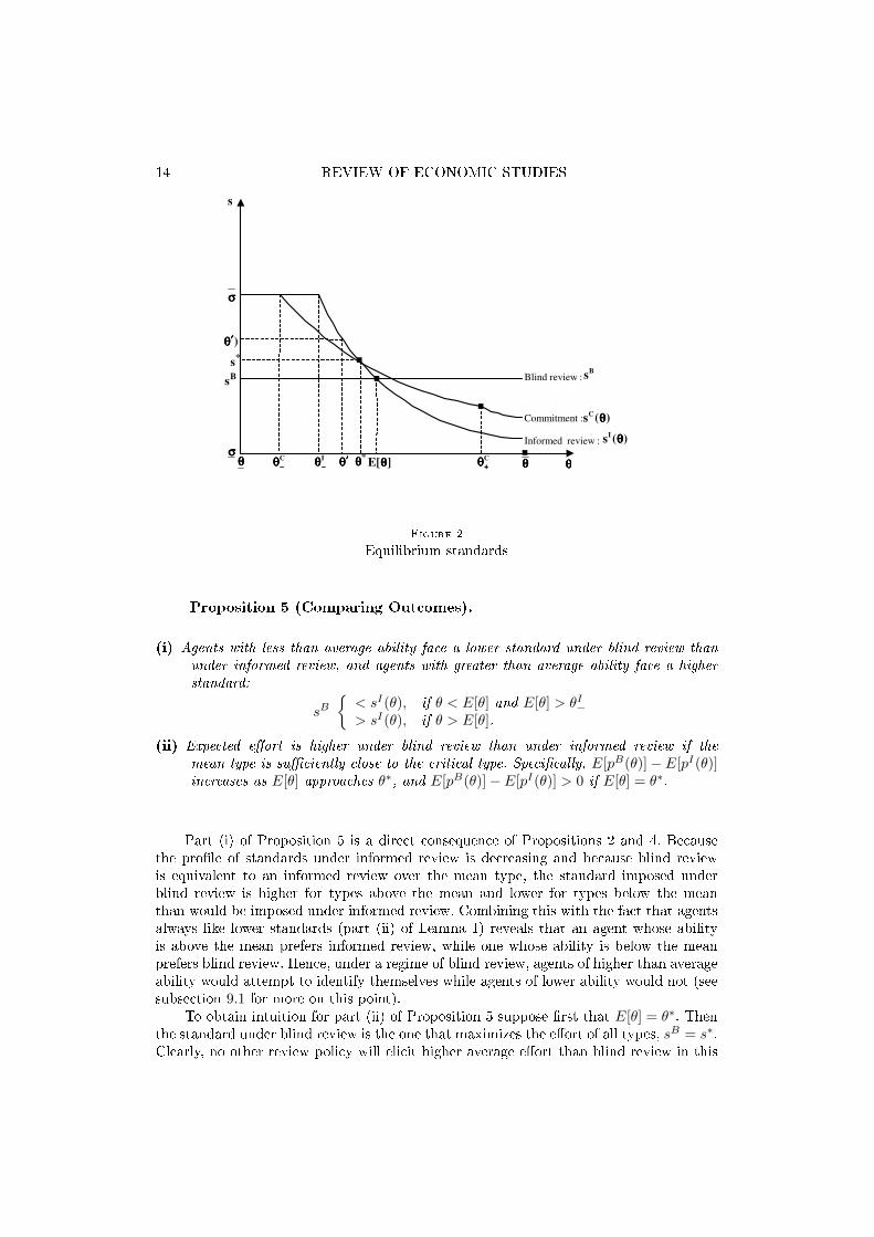
If the principal observes only a subjective signal of project quality, then she will notbe able to commit to the relatively �at pro�le of standards sC(θ). Nevertheless, in thiscase, it may be possible for her to commit to remain ignorant of the agent's type whenperforming an evaluation. That is, she may be able to implement a policy of blind reviewand impose the same completely �at standard sB on all types of agent (see Figure 2).While blind review forces the principal to disregard information that is valuable forproject selection, it can be an e�ective method for providing incentives. For instance, ablind review procedure with sB = s∗ would raise the e�ort of all types relative to a policyof informed review. Of course, even under blind review the principal can only implementa standard, sB , that is ex post optimal given the information she possesses. The questionis whether it is ever advantageous for her to commit to possessing less information.

In order to investigate blind review, it is analytically convenient to rule out cases inwhich the upward feasibility restriction on e�ort binds. Hence, the following additionalassumption is imposed below.12

Assumption 3 (Bounded E�ort). The highest ability agent never exerts fulle�ort,

θu(Fl(s∗)− Fh(s∗)) < 1.

Because the principal does not observe θ, the equilibrium standard is a best responseto the agent's expected e�ort:

sB = L−1(r

1− E[pB(θ)]

E[pB(θ)]

). (6.13)

Similarly, the agent's e�ort is a best response to the standard,

pB(θ) = θu(Fl(sB)− Fh(sB)). (6.14)

Finally, taking the expectation of (6.14) over θ gives

E[pB(θ)] = E[θ]u(Fl(sB)− Fh(sB)). (6.15)

These three equations de�ne the equilibrium standard and e�ort under blind review.Comparing the solution to (6.13), (6.14), and (6.15) to the solution to (4.2) and (5.10)yields the following characterization.

Proposition 4 (Equilibrium under Blind Review).

Principal: The principal sets the standard equal to the one she would have set for themean type of agent under informed review, sB = sI(E[θ]).

Agent: The agent chooses e�ort level pB(θ) = P (sI(E[θ]), θ).

While this result derives technically from linearity of the agent's reaction functionin θ and linearity of the principal's objective in p, it, nevertheless, seems intuitive that� when ignorant of the agent's type � the principal would set a standard as if she facedthe average type in the population (see Figure 2).

The following result provides a comparison between the standards and induced e�ortunder informed and blind review.

12. A stronger assumption, which is easier to check, is simply θu ≤ 1.


.

σσσσ

θθθθ

*s

θθθθ

σσσσ

*θθθθ

.

s

]E[θθθθ

.Bs

:review Informed

:Commitment

I

−−−−θθθθ

C

−−−−θθθθ

C

++++θθθθ

.

θθθθ

Standards mEquilibriu :2 Figure

:reviewBlind

θθθθ′′′′

)(sI

θθθθ′′′′

Bs

)(sC

θθθθ

)(sI

θθθθ

Figure 2

Equilibrium standards

Proposition 5 (Comparing Outcomes).

(i) Agents with less than average ability face a lower standard under blind review thanunder informed review, and agents with greater than average ability face a higherstandard:

sB{< sI(θ), if θ < E[θ] and E[θ] > θI−> sI(θ), if θ > E[θ].

(ii) Expected e�ort is higher under blind review than under informed review if themean type is su�ciently close to the critical type. Speci�cally, E[pB(θ)]− E[pI(θ)]increases as E[θ] approaches θ∗, and E[pB(θ)]− E[pI(θ)] > 0 if E[θ] = θ∗.

Part (i) of Proposition 5 is a direct consequence of Propositions 2 and 4. Becausethe pro�le of standards under informed review is decreasing and because blind reviewis equivalent to an informed review over the mean type, the standard imposed underblind review is higher for types above the mean and lower for types below the meanthan would be imposed under informed review. Combining this with the fact that agentsalways like lower standards (part (ii) of Lemma 1) reveals that an agent whose abilityis above the mean prefers informed review, while one whose ability is below the meanprefers blind review. Hence, under a regime of blind review, agents of higher than averageability would attempt to identify themselves while agents of lower ability would not (seesubsection 9.1 for more on this point).

To obtain intuition for part (ii) of Proposition 5 suppose �rst that E[θ] = θ∗. Thenthe standard under blind review is the one that maximizes the e�ort of all types, sB = s∗.Clearly, no other review policy will elicit higher average e�ort than blind review in this


case. Next, suppose (as depicted in Figure 2) that E[θ] is slightly greater than θ∗.13 ThensB = sI(E[θ]) will be less than s∗. For types θ > E[θ], blind review still imposes a higherstandard than informed review, so these types would continue to exert more e�ort underblind review. Types in the interval [θ∗, E[θ]), however, would exert more e�ort underinformed review because it calls for a higher standard, sI(θ) ∈ (sB , s∗]. Of course, sB isalso too low for a neighborhood of types less than θ∗. However, there is a type θ′ < θ∗

(shown in Figure 2) for whom the excessively low standard sB would elicit the same e�ortas the excessively high one sI(θ′) > s∗. For all types θ < θ′, blind review would inducestrictly higher e�ort. In other words, if E[θ] 6= θ∗, then there is a band of types aroundθ∗ who would exert more e�ort under informed review while the types outside this bandwould exert more e�ort under blind review. If E[θ] is distant from θ∗, then the bandof types who work harder under informed review is large, and it is clearly the superiorevaluation procedure because it provides both better selection and better incentives.

It is worth remarking on the reason blind review provides better incentives thaninformed review when E[θ] is close to θ∗. Under informed review, high-ability agents reston their laurels, knowing that the principal will give them the bene�t of the doubt. Low-ability agents also exert little e�ort under informed review, but for the opposite reason �they know that the principal will discriminate against them. Blind review pools high andlow ability agents together and improves incentives at both ends of the type spectrum.

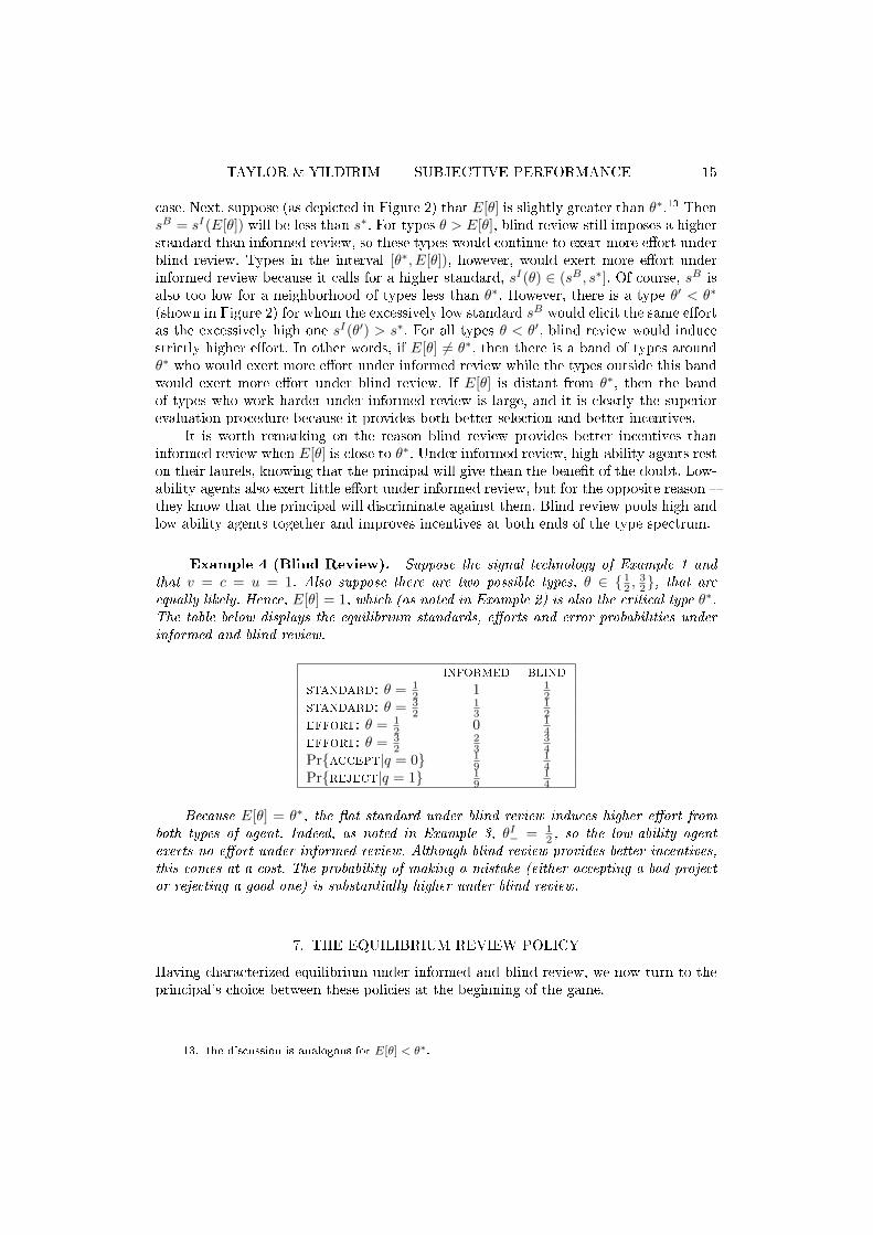
Example 4 (Blind Review). Suppose the signal technology of Example 1 andthat v = c = u = 1. Also suppose there are two possible types, θ ∈ { 12 ,

32}, that are

equally likely. Hence, E[θ] = 1, which (as noted in Example 2) is also the critical type θ∗.The table below displays the equilibrium standards, e�orts and error probabilities underinformed and blind review.

informed blind

standard: θ = 12 1 1

2standard: θ = 3

213

12

effort: θ = 12 0 1

4effort: θ = 3

223

34

Pr{accept|q = 0} 19

14

Pr{reject|q = 1} 19

14

Because E[θ] = θ∗, the �at standard under blind review induces higher e�ort fromboth types of agent. Indeed, as noted in Example 3, θI− = 1

2 , so the low-ability agentexerts no e�ort under informed review. Although blind review provides better incentives,this comes at a cost. The probability of making a mistake (either accepting a bad projector rejecting a good one) is substantially higher under blind review.

7. THE EQUILIBRIUM REVIEW POLICY

Having characterized equilibrium under informed and blind review, we now turn to theprincipal's choice between these policies at the beginning of the game.

13. the discussion is analogous for E[θ] < θ∗.


7.1. The Ability Distribution

De�ne the principal's equilibrium payo� under informed review by V I(θ) ≡V (sI(θ), pI(θ)). By proposition 4 the principal's expected equilibrium payo� under blindreview is

E[V B(θ)] = vE[pB(θ)](1− Fh(sB))− c(1− E[pB(θ)])(1− Fl(sB))

= vpI(E[θ])(1− Fh(sI(E[θ])))− c(1− pI(E[θ]))(1− Fl(sI(E[θ])))

= V I(E[θ]).

Therefore, when choosing between review policies, the principal compares her expectedpayo� under informed review, E[V I(θ)], with her expected payo� under blind review,V I(E[θ]). Evidently, if V I(·) is convex or concave everywhere, then Jensen's inequalitywill su�ce to rank the two payo�s irrespective of the type distribution. In general,however, V I(·) is S-shaped, possessing both a convex and a concave region, as thefollowing lemma records.

Lemma 2. If θI− is su�ciently low, then there exist two cutpoints, θL ≤ θH , suchthat V I(θ) is strictly convex for θ < θL and strictly concave for θ > θH .

The intuition behind Lemma 2 is that for very high types, e�ort is close to itsmaximum, and so is the principal's payo�. Thus, there are diminishing marginal returnsto ability. For very low types, on the other hand, a rise in ability not only raises e�ortbut signi�cantly improves the probability of making a correct acceptance decision.

In light of Lemma 2, it is clear that the principal's choice between the two reviewprocedures depends crucially on the distribution of types. If, for instance, all typesreceiving positive probability under g(·) are above θH (where V I(·) is concave), thenJensen's inequality implies that blind review dominates informed review. On the otherhand, if g(·) puts weight only on types less than θL (where V I(·) is convex), thenthe principal prefers informed review. More generally, determination of which reviewprocedure is optimal depends on whether high types or low types are more prevalent inthe population, as is stated in the following result.

Proposition 6 (Extreme Types and the Agent's Payo�). Suppose that thesupport of the ability distribution includes both the (low) region where V I(·) is convexand the (high) region where it is concave; i.e., θ < θL ≤ θH < θ. Then,

(i) there exist εB and εI > 0 such that the principal prefers blind review if G(θH) < εB,and informed review if G(θL) > 1− εI ; and

(ii) there exist 0 < uL ≤ uH <∞ such that the principal prefers blind review if u > uH ,and informed review if u < uL.

Part (i) of Proposition 6 indicates that incentives are more important than projectselection when evaluating high-ability agents, so blind review is optimal. Project selection,however, becomes the dominant concern when evaluating low-ability agents, and informedreview is, therefore, preferable in this case.

The second part of Proposition 6 states that, �xing the ability distribution, theprincipal is also more likely to prefer blind review, as the agent's payo� from acceptance,u, increases. Note from (4.2) that an increase in u is equivalent to an increase in θ.


Hence, agents with high rewards from acceptance will behave like those with high ability,in which case blind review is the principal's preferred mode of evaluation.

A question that naturally arises in light of Proposition 6 is whether blind reviewis the preferable evaluation process only when the ability distribution places su�cientweight on high values of θ. Mathematically this comes down to asking whether V I(θ) isconcave only at high ability levels. The following result establishes that this is not so.

Lemma 3. The principal's equilibrium payo� function V I(θ) is strictly concaveat θ∗.

Observe from (4.8) that θ∗ does not depend on the ability distribution. In particular,it is increasing in the principals cost to bene�t ratio r and decreasing in the agent's payo�from acceptance u and in the di�erence Fl(s

∗) − Fh(s∗). Hence, V I(θ) may possess aconcave region at virtually any point in the type space. It follows, therefore, that it isnot necessary for the ability distribution to include a large fraction of high types in orderfor blind review to be optimal. This is formalized as follows.

Proposition 7 (Non-Extreme Types). There exist ε > 0 and ∆ > 0 such thatif |E[θ]− θ∗| < ε and |θ − θ∗| < ∆ for all θ ∈ [θ, θ], then the principal prefers blindreview.

From part (ii) of Proposition 5, expected e�ort is higher under blind review thanunder informed review when the critical type is close to the mean. Moreover, whenthe support of the ability distribution is concentrated around θ∗, then observing therealization of θ is of little value to the principal, and blind review is, therefore, optimal.

Example 5 (Optimal Review). Suppose the signal technology of Example 1and that v = c = u = 1. From Example 3 it is straightforward to compute

V I(θ) =

(1− 1

2θ

)2

.

This is S-shaped, with an in�ection point at θH = θL = 34 . In accordance with Proposition

6, blind review is optimal for any ability distribution with θ ≥ 34 , and informed review is

optimal for any distribution with θ ≤ 34 . In accordance with Proposition 7, blind review is

also optimal for any distribution su�ciently concentrated around the critical type θ∗ = 1.If, as in Example 4, there are two types, θ ∈ { 12 ,

32}, that are equally likely, then the

principal's expected equilibrium payo�s under informed and blind review are respectivelyE[V I(θ)] = 2

9 and V I(E[θ]) = 14 .

7.2. The Informativeness of the Signal

An important element in determining the optimal review process is the informativenessof the signal observed by the evaluator. The informativeness of the signal varies acrossapplications depending on such factors as the expertise of the evaluator and the stageat which the project is submitted for review. In what follows, we de�ne a notion ofinformativeness based on MLRP along the lines suggested by Milgrom (1981), and theninvestigate its e�ect on the choice of the review policy.

Let α ∈ R+ be a parameter measuring the informativeness of the signal, and writethe probability distribution and corresponding density functions respectively as Fq(σ;α)


and fq(σ;α), for q = h, l. Intuitively, a signal technology is more informative if it ismore likely to generate a high signal when project quality is high, and a low signal whenproject quality is low. This is formalized as follows.

De�nition 1 (Informativeness). Signal technology {fh(σ;α1), fl(σ;α1)} is

said to be more informative than {fh(σ;α0), fl(σ;α0)} if fh(σ;α1)fh(σ;α0)

increases and fl(σ;α1)fl(σ;α0)

decreases in σ whenever α1 > α0.

That is, in addition to Assumption 1, we also impose MLRP separately on bothfh(σ;α) and fl(σ;α).

Next, normalize α so that as α → 0, the signal technology becomes completelyuninformative, namely Fl(σ;α) − Fh(σ;α) → 0 for all σ; and as α → ∞, it becomescompletely informative, namely Fl(σ;α)→ 1 for σ 6= σ, and Fh(σ;α)→ 0 for σ 6= σ. Inparticular, when the signal technology is completely informative, the principal observesonly the highest signal, σ, if project quality is high, and only the lowest signal, σ, if it islow. Finally, in order to compare di�erent signal technologies, it is necessary to impose

an assumption on the likelihood ratio, L(σ;α) ≡ fh(σ;α)fl(σ;α)

.

Assumption 4 (The Neutral Signal). L(s∗;α) = 1, for all α ∈ (0,∞).

In other words, s∗ continues to be the unique neutral signal, independent of α. Thisassumption implies that, as α increases, L(σ;α) rotates counter-clockwise around thepoint (s∗, 1) such that, as α → ∞, L(σ;α) → 0 if σ < s∗ and L(σ;α) → ∞ if σ > s∗.(see Lemma A1 in the Appendix).

A simple parametric extension of the signal technology presented in Example 1satis�es De�nition 1 and Assumption 4. Namely, it is straightforward to check that thefamily of signal technologies with fl(σ;α) = (1 + α)(1 − σ)α and fh(σ;α) = (1 + α)σα,for σ ∈ [0, 1] and α ≥ 0, works.

The �rst result of this subsection reveals that a more informative signal elicits greatere�ort from the agent.

Lemma 4. Suppose pI(θ;α) > 0.

(i) pI(θ;α) strictly increases in α.(ii) As α→ 0, pI(θ;α)→ 0 and sI(θ;α)→ σ for all θ.(iii) As α→∞, pI(θ, α)→ min{θu, 1} and

sI(θ;α)→{s∗, if θu < 1σ, if θu ≥ 1.

A more informative signal provides a tighter measure of the agent's performanceand improves incentives. In the extreme cases, the agent exerts no e�ort when the signalis completely uninformative, and the maximum e�ort when it is completely informative.An implication of this observation is that the principal is indi�erent between blind andinformed review, in either of the extreme cases (α = 0 or α =∞). For signal technologiesnear � but not equal to � the extremes, however, the principal has a strict preference foreither blind or informed review, as is stated in the following key result.

Proposition 8 (Informativeness). Suppose θu < 1. Then,


(i) When the signal technology is either completely uninformative or completely infor-mative, the principal is indi�erent between blind and informed review. In partic-ular, limα→0E[V I(θ;α)] = limα→0E[V B(θ;α)] = 0, and limα→∞E[V I(θ;α)] =limα→∞E[V B(θ;α)] = E[θ]vu.

(ii) For a su�ciently uninformative signal technology, the evaluator prefers informedreview. That is, for a small α > 0, E[V I(θ;α)] > E[V B(θ;α)].

(iii) For a su�ciently informative signal technology, the evaluator prefers blind review.That is, for a large α <∞, E[V I(θ;α)] < E[V B(θ;α)].

When the signal is imprecise, the principal opts to use the information containedin the agent's type to improve her selection decision; i.e, she uses informed review. Onthe other hand, when the signal is very precise, the principal eschews the informationcontained in the agent's type in order to provide better incentives; i.e., she uses blindreview.

8. APPLICATIONS

The analysis presented in the preceding section can be applied to address questionsregarding the equilibrium review policy in a variety of real-world settings. This isillustrated below in two examples: admission of character evidence in trials and academicrefereeing. There are, of course, aspects of these settings not captured by our model. Forinstance, in the case of a criminal trial, the principal (jurist) might also be concernedwith the future trajectory of the agent (defendant), not just his current conduct. In thecase of academic refereeing, the choice of review process also in�uences the evaluator'sincentives to perform a thorough evaluation. These important caveats notwithstanding,we believe that the analysis performed above sheds important light on these as well asother real-world evaluation settings.

8.1. Character Evidence in Trials

There is a long-standing debate among legal scholars about whether character evidence� i.e., the past conduct (good or bad) of the defendant � should be admissible at trial.Those who oppose the use of character evidence argue: (1) an individual's past behavioris too weak a predictor of his current act; (2) the Jury may be prone to �cognitive error,�giving too much weight to dispositional evidence; (3) Jurors might convict someone solelybased on his bad character or his prior wrongdoings; (4) the court's resources should notbe used on examining the details of someone's past; (5) banning character evidence forcesparties to seek the best evidence for the current case.

Legal scholars who support the use of character evidence argue that the defendant'spast acts may be a good predictor of the current act, because several in�uential studiesin social psychology maintain the stability of criminal behavior associated with certainpersonality features, such as lack of self-control or low-empathy. Moreover, supportersof character evidence say that it may be of use in tailoring incentives to individualcharacteristics. Character evidence would be of use in determining defendants' criminalpropensity, so that punishments could be appropriately adjusted.

The intellectual schism in the legal community over the admissibility of characterevidence appears to extend even to the U.S. Federal Rules of Evidence.14 For instance,

14. See http://www.law.cornell.edu/rules/fre/rules.htm.


opposing its use, Rule 404(b) states, �Evidence of other crimes, wrongs, or acts is notadmissible to prove the character of a person in order to show action in conformitytherewith.� Conversely, supporting its use, Rule 406 states, �Evidence of the habit ofa person or of the routine practice of an organization, whether corroborated or notand regardless of the presence of eyewitnesses, is relevant to prove that the conduct ofthe person or organization on a particular occasion was in conformity with the habitor routine practice.� In general, courts allow character evidence if its probative valueexceeds its prejudicial e�ect.15

In the context of the model presented above, one can think of the principal as a juristand the agent as a defendant in a trial. Initially (before the trial), the defendant exertssome e�ort p to avoid criminal behavior. The cost of this e�ort depends on the defendant'scharacteristics such as his education, age, and employment status, as summarized by θ.Project acceptance corresponds to acquittal and rejection to conviction. If characterevidence is admissible, then the jurist performs an informed review, and if it is banned,then she performs a blind review.

The close correlation between an individual's socioeconomic characteristics and thetype of crime he is most likely to commit is well documented.16 Speci�cally, blue-collar orstreet crimes, such as robbery and assault, tend to be committed by individuals who arerelatively young, uneducated, and poor (low values of θ), while white-collar or corporatecrimes, such as embezzlement or price �xing, tend to be committed by individuals whoare relatively old, educated, and wealthy (high values of θ). In this light, Proposition6 suggests that character evidence should be permitted in cases of street crime andeschewed in cases of white-collar crime. Interestingly, this analysis indicates that the over-riding concern in cases of blue-collar crime is making a correct decision about whetherto acquit or convict, while the predominant concern in cases of white-collar crime isdeterrence.

8.2. Journal Submissions and Grant Proposals

As a second application of the theory, note that Bachand and Sawallis (2003) �nd that58% of 553 journals across 18 academic disciplines use blind review of manuscripts; i.e.,the referee is not informed of the author's identity.17 Grant proposals, however, appearto always be evaluated non-blindly. Indeed, in many if not most cases (e.g., NSF, NIH,Russell Sage Foundation, Alfred P. Sloan Foundation) principal investigators are requiredto submit a Curriculum Vitae to be reviewed as part of their proposal.

A major di�erence between a journal submission and a grant proposal is the stageat which the research is evaluated. Grant proposals, by their nature, are speculative andpreliminary. They contain few, if any, concrete �ndings. Rather, they are hypothetical inscope and generally provide only a conceptual plan, or road map, for how the proposedresearch is to be performed. Journal submissions, by contrast, are intended to disseminate

15. For an excellent discussion of the alternative views on character evidence, see Sanchirico (2001).Also see Lippke (2008), and, for the British perspective, Redmayne (2002).

16. On the age distribution of crime, see Ste�ensmeier et al. (1989). On the link between economicinequality and violent crime see Blau and Blau (1982), and on the correlation between education andcrime see Ehrlich (1975), and Lochner and Moretti (2004).

17. In disciplines such as economics, where working papers are customarily uploaded to the web,commitment to blind review is not possible because a referee can ascertain the author's identity bysearching for a few key words. Perhaps this is why over 80% of the top-50 economics journals no longerattempt to practice blind review. Many disciplines, however, do not post manuscripts on the Internet,making blind review still a feasible option.


actual research �ndings. They are supposed to contain substantial analysis and explicitresults.

It stands to reason, therefore, that the signal an evaluator receives about theultimate quality of the research is much less informative when reviewing a grant proposalthan when reviewing a journal submission. Proposition 8 accords neatly with thisinterpretation. Grant proposals, which are submitted at a very early stage of the project,should be subjected to informed review, while manuscripts, which are submitted at amore mature stage, should be reviewed blindly. In other words, the primary concern ingrant review should be the selection of good projects, while the dominant concern inmanuscript review should be the provision of incentives for authors to write high-qualitypapers.

9. GENERALIZATIONS AND EXTENSIONS

In this section, the basic model is extended in three dimensions to highlight the robustnessof the results obtained above and glean some important additional insights.

9.1. Competing Evaluators and Informed Review Bias

In practice there are often multiple evaluators (e.g., schools, companies, and academicjournals) that compete for high-quality applications. In this subsection, the basic modelis extended to show how competition among evaluators impacts the equilibrium mode ofreview.

Suppose there are two ex ante symmetric evaluators, i = 1, 2, who simultaneouslyand publicly announce their review policies, τi ∈ {I,B}. Upon observing τ1 and τ2,each agent then exerts e�ort and applies to one evaluator. To parameterize the degreeof competition, one of three possible situations is assumed to obtain. With probability1−φ an agent is unattached (i.e., he is free to apply to either evaluator); with probabilityφ2 he is attached to evaluator 1; and with probability φ

2 he is attached to evaluator 2.Attachments are independent across agents and over types. For simplicity, also assumethat re-applications are not feasible, and, in case of indi�erence, an unattached agentselects between the evaluators with equal probability.

Let πτ1,τ2i be evaluator i's expected payo� in the subgame with review policiesτ1 and τ2. Note that, if τ1 = τ2 = I, then ex ante each agent is equally likely toapply to either evaluator, resulting in equal payo�s, πI,Ii = 1

2E[V I(θ)]. Similarly, ifτ1 = τ2 = B, then a straightforward argument shows that, in equilibrium, both evaluatorsadopt the same standard tailored to the population mean, E[θ], yielding equal payo�s,

πB,Bi = 12V

I(E[θ]). The equilibrium characterization with di�erent review policies is lessobvious.

Suppose τ1 = B and τ2 = I. Moreover, suppose, in equilibrium, the mean type thatapplies to evaluator 1 is m1. This implies that an unattached type θ prefers evaluator 1whenever θ < m1. Hence, the conditional mean ability for evaluator 1 is

M1(m1;φ) ≡(1− φ

2 )∫m1

θθ dG(θ) + φ

2

∫ θm1

θ dG(θ)

(1− φ2 )G(m1) + φ

2 (1−G(m1)).

In equilibrium, the conditional mean, m1 = µ1(φ), must solve

M1(m1;φ)−m1 = 0. (9.16)


Lemma 5. There exists a unique solution, µ1(φ) to (9.16). The function µ1(φ)is strictly increasing and has boundary values µ1(0) = θ and µ1(1) = E[θ].

Lemma 5 says that as each agent becomes less likely to be attached, fewer high typesapply to evaluator 1 for blind review. This causes it to raise its standard and furtherdiscourages applications by high unattached types in the remaining pool. In particular,in the absence of attached types (φ = 0), complete unraveling occurs and all agents applyto evaluator 2 for informed review.

In light of Lemma 5, equilibrium payo�s for evaluators 1 and 2 in the subgame withτ1 = B and τ2 = I are given, respectively, by

πB,I1 (φ) =

[(1− φ

2

)G(µ1(φ)) +

φ

2(1−G(µ1(φ)))

]V I(µ1(φ))

and

πB,I2 (φ) =φ

2

∫ µ1(φ)

θ

V I(θ) dG(θ) +

(1− φ

2

)∫ θ

µ1(φ)

V I(θ) dG(θ).

The following lemma characterizes these payo�s.

Lemma 6. In the unique equilibrium with τ1 = B and τ2 = I, the evaluator'spayo�s have the following properties:

(i) πB,I1 (φ) is strictly increasing, and πB,I1 (0) = 0 and πB,I1 (1) = 12V

I(E[θ]).

(ii) πB,I2 (φ) is strictly decreasing, and πB,I2 (0) = E[V I(θ)] and πB,I2 (1) = 12E[V I(θ)].

In other words, the evaluator who uses blind review is better o� when there aremore attached types, because they have a direct positive e�ect on her payo� as well asa positive indirect e�ect through attracting high unattached types, who, by Lemma 5,anticipate a lower standard. By the same token, the evaluator who uses informed reviewis worse o� when there are more attached types.

Having characterized the evaluators' payo�s in each subgame, the equilibrium reviewpolicies can now be determined.

Proposition 9 (Equilibrium with Competing Evaluators). Suppose12V

I(E[θ]) < E[V I(θ)] < V I(E[θ]). Then, there exist two cutpoints, 0 < φ∗ ≤ φ∗∗ < 1,such that for φ < φ∗, the unique equilibrium has τ1 = τ2 = I, whereas for φ > φ∗∗, theunique equilibrium has τ1 = τ2 = B. For φ ∈ [φ∗, φ∗∗], both symmetric and asymmetricreview policies may occur in equilibrium.

The message of Proposition 9 is that competition among evaluators to attract highquality applications is likely to lead them to adopt informed review, even when eachwould individually prefer blind review.

9.2. Two Types of Error

Up to now, it has been assumed that the evaluator su�ers a loss only from a falseacceptance. In some settings, however, she may also su�er a loss from a false rejection. Forinstance, misjudging a potentially good musician is probably as costly for the performanceof a symphony orchestra as hiring a potentially bad one. In Taylor and Yildirim (2007) it


is shown that accounting for both types of error does not qualitatively change the mainresults derived from the basic model, especially those pertaining to the comparison ofinformed and blind review. Thus, in this subsection only the novel insights associatedwith this generalization are highlighted.

Suppose, in addition to the loss −c < 0 from a false acceptance, the principal alsoincurs a loss −c < 0 from a false rejection. While this does not alter the agent's payo�in (4.1), the expected loss from rejecting a good project needs to be subtracted from theprincipal's payo� in (4.3):

V (s, p) = vp(1− Fh(s))− c(1− p)(1− Fl(s))− cpFh(s). (9.17)

Maximizing (9.17) with respect to s, the principal's reaction function is

S(p) = L−1(r

1− pp

), (9.18)

where r ≡ cv+c . Because L

′ > 0, (9.18) implies that the principal is more likely to accepta project as her loss from a false rejection increases. Applying the Envelope Theorem,the principal's indirect payo� satis�es

d

dpV (S(p), p) = v(1− Fh(S(p))) + c(1− Fl(S(p)))− cFh(S(p)),

which is clearly positive if S(p) is close to σ, and negative if S(p) is close to σ. Hence, incontrast to part (i) of Lemma 1, the principal's indirect payo� does not monotonically

increase in p. In fact, since S(0) = σ and S′(p) < 0, her indirect payo� strictly decreases

in p whenever p is small, because such a project is very likely to be rejected, and thusexposes the principal to risk of false rejection.18 In fact, a su�ciently small p may resultin a negative payo� for the evaluator, V (S(p), p) < 0, which never occurs in the basemodel. The evaluator would, of course, avoid a negative payo� if she could commit toprescreening those agents who are unlikely to exert a high enough e�ort. Intuitively, inthe absence of commitment by the principal, some low-ability agents will take advantageof her fear of false rejections by submitting projects with very low values of p.

The discussion thus far suggests two novel insights that are con�rmed in Proposition10: �rst, the evaluator may receive a negative equilibrium payo� from some intermediatetype agents, and second, there may be too little equilibrium prescreening compared withthe commitment benchmark.

Proposition 10 (Two Types of Error). Suppose both types of error are costlyto the evaluator, i.e., c, c > 0. Then, in equilibrium,

(i) under informed review there exist two types, θI

− < θI

r, such that

V (θ)

= 0 if θ ≤ θI− or θ = θ

I

r

< 0 if θI

− < θ < θI

r

> 0 if θ > θI

r ,

(ii) if c is su�ciently large, then, compared with commitment, there is less prescreening

under informed review, namely, θI

− < θC

−.

18. The nonmonotonicity of the evaluator's indirect payo� implies that equilibria under informedreview are not always Pareto rankable. For consistency, we continue to assume that the players coordinateon the equilibrium with the highest e�ort and lowest standard.


Hence, when the evaluator is su�ciently concerned about a false rejection, there maybe too little prescreening under informed review as opposed to too much prescreening asobserved in the base model. The reason is as suggested above: when the evaluator fearsrejecting a good project, she cannot credibly discourage some intermediate type agentsfrom submitting projects in equilibrium, even though they are unlikely to produce highquality.

9.3. Non-Productive E�ort

In some settings, applicants can engage in both productive activities, which enhance theircurrent performance, and in�uence activities, which may enhance the signal receivedby the evaluator but do not enhance the actual quality of the project. For instance,an individual submitting a manuscript for publication may spend signi�cant time andenergy on formatting and layout, rather than on improving content. To capture thispossibility, extend the base model by supposing that an agent can exert two kinds ofe�ort: a productive e�ort, p, and an unproductive e�ort, e. In particular, even when thetrue quality of the project is low, which happens with probability 1 − p, the evaluatorstill receives the signal from Fh with probability e. In this case, the principal's expectedpayo� is given by

V (s, p, e) = p(1− Fh(s))v − e(1− p)(1− Fh(s))c− (1− e)(1− p)(1− Fl(s))c.

Di�erentiating with respect to s yields

Vs(s, p, e) = [(−p+ (1− p)er)L(s) + (1− p)(1− e)r]vfl(s).

Note that if −p+(1−p)er ≥ 0, then S(p, e) = σ. Suppose −p+(1−p)er < 0. Then,the evaluator's reaction function is

L(S(p, e)) =(1− p)r − (1− p)er

p− (1− p)er.

For e = 0 this yields the base-model reaction function.As for the agent, assume that ability a�ects only the cost of exerting productive

e�ort. That is, all types of agent are equally capable of in�uence activity.19 In particular,

a type θ agent's cost of exerting p and e is 12

(p√θ

+ e√t

)2, where t > 0 is a constant.

Hence his expected utility is

U(p, e, s; θ) = u[(1−(1−p)(1−e))(1−Fh(s))+(1−p)(1−e)(1−Fl(s))]−1

2

(p√θ

+e√t

)2

.

This also yields the base model when e = 0.

Lemma 7. For any s ∈ [σ, σ], the best response of a type θ agent is as follows:for θ ≤ t, p = 0 and e = min{tu(Fl(s) − Fh(s)), 1}, and for θ ≥ t, e = 0 andp = min{θu(Fl(s)− Fh(s)), 1}.

The agent's payo� function is submodular in the two kinds of e�ort (Upe < 0), sothe marginal return to productive e�ort is highest when non-productive e�ort is zero and

19. Technically, what matters is that in�uence ability not be perfectly correlated with productiveability.


vice versa. If θ < t, then non-productive e�ort costs the agent less than productive e�ort,and if θ > t, then the reverse is true.

Clearly, under informed review the principal will prescreen all types θ < t; i.e.,s = σ and p = e = 0. For θ ≥ t, the equilibrium is as characterized in Proposition 2,namely s = sI(θ) and p = pI(θ). The equilibrium under blind review is more di�cult tocharacterize, mainly because the equilibrium standard sB is a function of t. In general,blind review should perform relatively poorly compared with informed review when non-productive e�ort is possible. Under informed review, low-ability agents who specialize innon-productive e�ort can be excised from the applicant pool, while under blind reviewthey cannot. The following result reveals that when there is a signi�cant fraction of agentswho exert non-productive e�ort, then blind review is infeasible.

Proposition 11 (Rent Seeking). Suppose θu ≤ 1. There exists t < θ such thatif t ≥ t, then blind review results in the degenerate equilibrium: sB = σ and pB = eB = 0.Hence, if t ∈ [t, θ), then informed review is optimal.

This result says that if the fraction of �spoilers� in the population is high enough(G(t) ≥ G(t)), then the principal would reject all projects under blind review. (As theproof of the proposition makes clear, t is decreasing in r, so that the fraction of spoilerscan be small if the cost to bene�t ratio is high.) However, so long as some fraction ofagents prefer to exert productive e�ort (G(t) < 1), the principal receives a positive payo�under informed review because she only evaluates submissions from agents with θ ≥ t.Hence, the ability of agents to exert non-productive e�ort mitigates against the adoptionof blind review.

10. CONCLUSION

The issue at the heart of this paper concerns the tradeo� between the e�ective use ofinformation and the provision of incentives, in a setting where commitment to a reviewstandard is infeasible. It was shown in this context that when the evaluator observesthe innate ability of the applicant, the equilibrium review policy is unduly biased �the standards facing high ability applicants are too weak and those facing low-abilityapplicants are too tough. While this policy uses information optimally ex post, it providespoor incentives ex ante. In particular, if the evaluator could commit to a review procedure,then she would implement a �atter (less biased) one. Commitment to such a policy is,however, often impractical or impossible because of the subjective nature of performancemeasures: the taste of a �ne wine, the skill of a classical musician, the preponderance ofevidence. Although it is not possible to commit to a highly tailored acceptance procedurein such environments, it is often possible to commit to remain ignorant of the identity(and hence the ability) of the applicant; that is, to perform blind review.

The uniform standard implemented under blind review often provides goodincentives for agents at both ends of the ability distribution, but it sacri�ces informationat the project selection stage. Hence, whether the evaluator prefers blind or informedreview depends critically on whether incentives or project selection is more important toher. Blind review was shown to be the preferred mode of evaluation if the applicant poolcontains a large proportion of high ability agents, the applicant's stakes from acceptanceare relatively high, the subjective signal of project quality is fairly precise, wrong decisionsare relatively less costly, or there is limited competition among evaluators.


Two applications were presented. In the context of criminal trials, the theorypresented here suggests that character evidence should be admissible in cases of streetcrime but not white-collar crime. It was also argued that research projects in early stagesof development (e.g., grant proposals) should be subjected to informed review, whileprojects in later stages (e.g., manuscripts) should be evaluated blindly.

There are a number of intriguing issues that remain to be addressed in future work.For instance, it would be interesting to investigate the e�ects of more general non-monetary incentive devices. In academia, for example, there is a gradation of rewardsassociated with acceptance of a manuscript (lead article, long or short paper, best paperprize, and so on) that can be used to induce individuals to exert more e�ort. Similarly, itwould also be interesting to study the role of peer e�ects in a setting where an applicant'sbene�t from acceptance, u, is determined endogenously. Speci�cally, the status or prestigeenjoyed by an agent whose project is accepted might well depend on the average qualityof other projects accepted by the evaluator. Another intriguing avenue for future researchwould be to consider the possibility of psychological bias on the part of the evaluatorand the role of blind review in mitigating prejudice. Finally, it would be instructive tostudy a dynamic version of the model in which the current ability of an agent depends onhis history of prior projects. In particular, it would be useful to explore the interactionbetween the review policies of evaluators and the career trajectories of agents in such asetting. While these and other topics for further research appear fruitful, it seems likelythat the fundamental message of this paper will remain intact. Fairness is not the onlyreason to level the playing �eld � often it is also the best thing the evaluator can do.

APPENDIX

This appendix contains the proofs of all lemmas and propositions presented in thetext, as well as the statement and proofs of two technical lemmas.

Proof of Proposition 1. Note �rst that if a type θ agent is subject to s su�cientlyclose to σ, then P (s, θ) < 1, and hence V (s, P (s, θ)) is strictly quasi-concave in sby Assumption 2. This means sC(θ) = σ if and only if lims→σ

ddsV (s, P (s, θ)) > 0.

Di�erentiating (4.4) and noting lims→σ P (s, θ) = 0 and lims→σ[L(s)P (s, θ)] = uθ(λh−λl)by Assumption 1, it follows sC(θ) = σ and thus pC(θ) = 0 if and only if θ <

ru[2λh+(r−1)λl] = θC−. Second, suppose P (s, θ) > 0. If we ignore the constraint P (s, θ) ≤ 1,

then by Assumption 2, sC(θ) = sC0 (θ) is the unique solution to ddsV (sC0 (θ), P (sC0 (θ), θ)) =

0, or equivalently to (4.5). If P (sC0 (θ), θ) > 1, then sC(θ) 6= sC0 (θ); rather sC(θ) =min{s|P (s, θ) = 1}, because for P (s, θ) = 1, (4.4) reduces to V (s, P (s, θ)) = v(1−Fh(sI)),which is strictly decreasing in s. By construction, sC(θ) is continuous for θ 6= θC−. Sincelims→σ V (s, p) = 0 for any p ∈ [0, 1], sC(θ) is also continuous at θ = θC−. This impliesthat pC(θ) = P (sC(θ), θ) is continuous for all θ.

To prove that sC(θ) is strictly decreasing for θ > θC−, observe that for θ ∈(θC−, θ

C+), d

dθ sC(θ) =sign Vp(·)Psθ(·) + Vsp(·)Pθ(·) by Assumption 2. Since Pθ(·) = P (·)

θ ,

and Vp(·)Psθ(·) =Vp(·)Ps(·)

θ = −Vs(·)θ (where the last equality is due to the FOC),the r.h.s. simpli�es to Vp(·)Psθ(·) + Vsp(·)Pθ(·) = 1

θ [Vsp(·)P (·) − Vs(·)]. From (4.3),Vs(s, p) = −pfh(s)v + (1 − p)fl(s)c and Vsp(s, p) = −[fh(s)v + cfl(s)], which implyVsp(·)P (·) − Vs(·) = −fl(s)c < 0. Hence, d

dθ sC(θ) < 0 for θ ∈ (θC−, θ

C+). For θ > θC+ ,

we have P (sC(θ), θ) = 1, and thus ddθ s

C(θ) = −Pθ(·)Ps(·) < 0, where Ps(·) > 0 because

sC(θ) < s∗ = L−1(1). For θ = θC+ , sC(θ) is not di�erentiable, but it is clearly strictly

decreasing. As a result, sC(θ) is strictly decreasing for all θ > θC−. Given that sC(θ)


is strictly decreasing and V (s, P (s, θ)) is strictly quasi-concave by Assumption 2 forθ ∈ (θC−, θ

C+), it easily follows that pC(θ) is strictly increasing for θ ∈ (θC−, θ

C+).

Finally, suppose, to the contrary, that limθ→∞ sC(θ) = sC > σ. Then, there would

be a su�ciently large θ < ∞ such that pC(θ) = 1 and sC(θ) > σ. But in this case,the principal could strictly improve her payo�, v(1 − Fh(s)), by setting a standard,

(sC(θ) + σ)/2. Hence, limθ→∞ sC(θ) = σ. ‖Proof of Lemma 1. Since, by de�nition, Vs(S(p), p) = Up(P (s, θ), s; θ) = 0, (4.1)

and (4.3) imply that ddsU(P (s, θ), s; θ) = ∂

∂sU(P (s, θ), s; θ) < 0 and ddpV (S(p), p) =

∂∂pV (S(p), p) > 0. ‖

Proof of Proposition 2. To prove the existence of the cuto� type θI−, observe thatV (s, p) is strictly quasi-concave in s because L′(s) > 0. This means sI(θ) = σ if and only iflims→σ Vs(s, P (s, θ)) > 0. Since lims→σ P (s, θ) = 0 and lims→σ L(s)P (s, θ) = uθ(λh−λl)by Assumption 1, we have sI(θ) = σ and thus pI(θ) = 0 if and only if θ < r

u(λh−λl) = θI−.

Next, note that pI(θ) < 1 for all θ < ∞; otherwise, if pI(θ) = 1 for some θ < ∞, then

sI(θ) = S(1) = σ, to which the agent would reply by pI(θ) = 0, contradicting pI(θ) = 1.Note also that pI(θ) < 1 implies that sI(θ) > σ for all θ <∞.

Now, we prove that sI(θ) is strictly decreasing for θ > θI−. Recall from the text that

sI(θ) = sI0(θ), which is the smallest root to (5.11), or equivalently to S−1(s, r)−P (s, θ) =

0, where S−1(s, r) ≡ S−1(L−1(r 1−pp )). Di�erentiating the last equation with respect toθ, we �nd

∂

∂θsI0(θ) =

Pθ(sI0(θ), θ)

S−1s (sI0(θ), r)− Ps(sI0(θ), θ).

Clearly, Pθ(sI0(θ), θ) = u[Fl(s

I0(θ)) − Fh(sI0(θ))] > 0 because pI(θ) = P (sI0(θ), θ) < 1.

To show that S−1s (sI0(θ), r) − Ps(sI0(θ), θ) < 0, note that S−1s (sI0(θ), r) < 0 by our

equilibrium selection, and thus S−1s (sI0(θ), r)−Ps(sI0(θ), θ) < 0 whenever Ps(sI0(θ), θ) ≥ 0.

Suppose that Ps(sI0(θ), θ) < 0 and, to the contrary, that S−1s (sI0(θ), r)−Ps(sI0(θ), θ) ≥ 0.

If S−1s (sI0(θ), r) − Ps(sI0(θ), θ) = 0 for some θ, then by continuity, there would be a

su�ciently small ε > 0 such that sI0(θ) = sI0(θ + ε). But, from (4.2), this wouldimply pI(θ) < pI(θ + ε), and thus sI0(θ) 6= sI0(θ + ε), yielding a contradiction. Hence,

S−1s (sI0(θ), r)−Ps(sI0(θ), θ) > 0. But then, by continuity, we would have S−1s (sI0(θ)−ε, r)−Ps(s

I0(θ) − ε, θ) < 0 for some ε > 0. Given S−1(σ, r) − P (σ, θ) > 0, this would generate

another equilibrium with a greater e�ort, contradicting our equilibrium selection. Thus,for θ > θI− and thus sI0(θ) 6= σ, it must be that S−1s (sI0(θ), r) − Ps(sI0(θ), θ) < 0. Hence,∂∂θ s

I0(θ) < 0.

Given that ∂∂θ s

I0(θ) < 0, and from (5.10) that pI(θ) = r

r+L(sI0(θ)), it immediately

follows∂

∂θpI(θ) = − rL′(·)

[r + L(·)]2∂

∂θsI0(θ) > 0.

Finally, to prove the limits as θ → ∞, suppose limθ→∞ pI(θ) → pI < 1. From(5.10), this would imply limθ→∞ sI0(θ) = σI > σ. But then, since Fl(σ

I) − Fh(σI) > 0,it must be that pI = 1 by (4.2), yielding a contradiction. Hence, pI = 1. As a result,limθ→∞ sI(θ) = σ. ‖

Proof of Proposition 3. Suppose θ > θC−. Since θC− < θI−, clearly s

C(θ) < sI(θ) =σ for θ ∈ (θC−, θ

I−). Next, note that θC+ > θ∗: otherwise, if θC+ ≤ θ∗, then there would be

some �nite θ ≥ θC+ for which pI(θ) = 1, contradicting Proposition 2.


Suppose θ < θ∗, but, on the contrary, sC(θ) = sC0 (θ) ≥ sI(θ). Since sI(θ) >sI(θ∗), it follows that Vs(s

I(θ), pI(θ)) = 0 and Ps(sI(θ), θ) < 0, which imply

ddsV (s, P (s, θ))

∣∣s=sI(θ)

< 0, and by Assumption 2 reveal sC(θ) < sI(θ) � a contradiction.

Thus, sC(θ) < sI(θ) for θ < θ∗. Given θC+ > θ∗, a similar line of argument showsthat sC(θ∗) = sI(θ∗), and sC(θ) > sI(θ) for θ∗ < θ ≤ θC+ . Finally, suppose θ > θC+ .Then, sC(θ) = min{s|P (s, θ) = 1} by Proposition 1. If, on the contrary, sC(θ) ≤ sI(θ),then since θ > θC+ , we would have 1 = P (sC(θ), θ) ≤ P (sI(θ), θ) because Ps(s, θ) > 0for θ > θC+ . But this would imply pI(θ) = 1, contradicting Proposition 1. Hence,sC(θ) > sI(θ) for θ > θC+ . Finally, to prove pC(θ) ≥ pI(θ) with strict inequality ifθ 6= θ∗, simply recall Ps(s, θ) =sign s∗ − s whenever P (s, θ) < 1. ‖

Proof of Proposition 4. The claim directly follows from (6.13), (6.14), and(6.15). ‖

Proof of Proposition 5. Since sI(θ) is strictly decreasing for θ > θI−, andsB = sI(E[θ]), part (i) immediately follows. To prove part (ii), note that Fl(s) − Fh(s)is strictly quasi-concave in s, achieving its unique maximum at s = s∗. Since sI(E[θ])is strictly decreasing, this implies that Fl(s

B) − Fh(sB) = Fl(sI(E[θ])) − Fh(sI(E[θ]))

is strictly quasi-concave in E[θ], admitting its maximum at E[θ] = θ∗. Thus, for agiven type θ, pB(θ) − pI(θ) strictly increases in E[θ] as E[θ] approaches θ∗, and sodoes E[pB(θ)]−E[pI(θ)]. Moreover, if E[θ] = θ∗ so that sB = s∗, then pB(θ)−pI(θ) > 0for all θ 6= θ∗ and pB(θ) − pI(θ) = 0 for θ = θ∗, revealing that E[pB(θ)] − E[pI(θ)] > 0at E[θ] = θ∗. ‖

Proof of Lemma 2. Consider θ > θI− so that pI > 0. We �rst prove the followingclaim.

Claim.pI′′

pI′sI′→∞, as θ →∞.

Proof. Since pI < 1 by Proposition 2, pI = θu(Fl(sI) − Fh(sI)). Di�erentiating

with respect to θ, we obtain

pI′ = u[(Fl(sI)− Fh(sI)) + θ(fl(s

I)− fh(sI))sI′]

and

pI′′ = u[(fl(sI)− fh(sI))(2sI′ + θsI′′) + (f ′l (s

I)− f ′h(sI))θ(sI′)2].

Again, by Proposition 2, we know pI → 1 and sI → σ as θ →∞. Suppose θsI′ → a <0. Then, pI′ → u[fl(σ)−fh(σ)]a < 0 because fl(σ)−fh(σ) > 0, which contradicts pI′ > 0.

Hence, θsI′ → 0, which implies sI′ → 0. Next, by de�nition pI′

θsI′= u[Fl(s

I)−Fh(sI)θsI′

+

fl(sI)−fh(sI)], and by L'Hopital's rule, limθ→∞

Fl(sI)−Fh(sI)θsI′

= limθ→∞(fl(s

I)−fh(sI))sI′sI′+θsI′′

.

This means for a su�ciently large θ, pI′

θsI′≈ u[fl(σ) − fh(σ)] 2s

I′+θsI′′

sI′+θsI′′. Since pI′

θsI′< 0,

fl(σ) − fh(σ) > 0 and sI′ < 0, we must have sI′ + θsI′′ > 0 and 2sI′ + θsI′′ < 0.Now, observe that since sI′ → 0 and sI′′ > 0, it follows sI′′ → 0. Using L'Hopital's

rule, sI′

sI′′≈ sI′′

sI′′′for a su�ciently large θ, implying that sI′′′ < 0. A similar limit

argument shows that Fl(sI)−Fh(sI)sI′

≈ [fl(σ)−fh(σ)]sI′sI′′

≈ [f ′l (σ)−f′h(σ)](s

I′)2+[fl(σ)−fh(σ)]sI′′sI′′′

.Given sI′′′ < 0, the numerator of the last ratio must be positive, or, equivalentlyf ′l (σ)−f

′h(σ)

fl(σ)−fh(σ) > −sI′′

(sI′)2. Next, consider the following ratio:

pI′′

pI′sI′=u[(fl(s

I)− fh(sI))(2sI′ + θsI′′) + (f ′l (sI)− f ′h(sI))θ(sI′)2]

pI′sI′.


Dividing the right side by θ(sI′)2, we obtain

pI′′

pI′sI′=

(fl(sI)− fh(sI)) 2sI′+θsI′′

θ(sI′)2+ f ′l (s

I)− f ′h(sI)

pI′

θsI′

u.

Thus, for a large θ

pI′′

pI′sI′≈

[fl(σ)− fh(σ)] 2sI′+θsI′′

θ(sI′)2+ f ′l (σ)− f ′h(σ)

[fl(σ)fh(σ)] 2sI′+θsI′′

sI′+θsI′′

u

=sI′ + θsI′′

θ(sI′)2u+

[f ′l (σ)− f ′h(σ)]

[fl(σ)− fh(σ)]

sI′ + θsI′′

2sI′ + θsI′′u

>sI′ + θsI′′

θ(sI′)2u− sI′′

(sI′)2sI′ + θsI′′

2sI′ + θsI′′u

=sI′ + θsI′′

2sI′ + θsI′′2

θsI′u = +∞,

where the last line follows because pI′ = − (pI)2L′

r sI′ and L′(σ) < ∞, revealingpI′

θsI′= − (pI)2L′

θr → 0− as θ → ∞. Furthermore, given pI′

θsI′≈ u[fl(σ) − fh(σ)] 2s

I′+θsI′′

sI′+θsI′′,

we have 2sI′+θsI′′

sI′+θsI′′→ −∞, which, together with 2

θsI′→ −∞, proves the claim. ‖

Now, in general

V I′′ = (VsssI′ + Vspp

I′)sI′ + VssI′′ + (Vpss

I′ + VpppI′)pI′ + Vpp

I′′.

Consider the right side of this expression. The �rst term is zero by straightforward (buttedious) algebra. Moreover, Vs = 0 by the principal's FOC and Vpp = 0 by linearity.Hence,

V I′′ = VpssI′pI′ + Vpp

I′′, (A1)

where Vps = −(fh(sI)v + fl(sI)c) and Vp = (1− Fh(sI))v + (1− Fl(sI))c.

If θ → θI−, then sI → σ, which implies Vps → −fh(σ)v − fl(σ)c < 0 and Vp → 0.

Hence, V I′′ > 0. Finally, for θ → ∞, we have sI → σ, Vps → −fh(σ)v − cfl(σ) < 0 and

Vp → v + c > 0. Moreover, since, by the earlier Claim, pI′′

pI′sI′→ +∞, the second term in

(A1) dominates, and given pI′′ < 0, implies V I′′ < 0.Overall, this establishes the existence of two cutpoints θI− < θL ≤ θH <∞ such that

V I(θ) is strictly convex for θ < θL and strictly concave for θ > θH . ‖

Proof of Proposition 6. Suppose θ < θL ≤ θH < θ, where θL and θH are thetwo cutpoints de�ned in Lemma 2, and by de�nition, they are independent of the typedistribution. Since V I(θ) is strictly concave for θ > θH , Jensen's inequality implies∫ θ

θH

V I(θ)dG(θ)

1−G(θH)< V I

(∫ θ

θH

θdG(θ)

1−G(θH)

),

or equivalently ∫ θ

θH

V I(θ)dG(θ) < (1−G(θH))V I

(∫ θ

θH

θdG(θ)

1−G(θH)

).


Then, by adding the term∫ θHθ

V I(θ)dG(θ) to both sides,

E[V I(θ)] < (1−G(θH))V I

µ(G(θH))−∫ θHθ

θdG(θ)

1−G(θH)

+

∫ θH

θ

V I(θ)dG(θ)

≤ (1−GH)V I(µ(GH)− θGH

1−GH

)+ V I (θH)GH ≡ Φ(GH),

where G(θH) ≡ GH and µ(GH) is the mean type given GH . For GH = 0, note thatE[V I(θ)] < V I(µ(0)) = Φ(0) because V I(θ) is strictly concave for θ > θH by hypothesis,and µ(0) > θH . Given that Φ(GH) is continuous, there must exist some εB > 0 suchthat E[V I(θ)] < V I(µ(GH)) whenever GH < εB . A similar line of argument showsthat there must also exist some εI > 0 such that E[V I(θ)] > V I(µ(GL)) wheneverGL ≡ G(θL) > 1− εI , completing the proof of part (i).

To prove the second part, �x a type distribution G(θ), and let θ ≡ uθ ∈ [uθ, uθ]

so that Gu(θ) = G( θu ). Clearly, Gu(θH) = G( θHu ) → 0 as u → ∞, which implies that

there is some uH > 0 such that Gu(θH) < εB for all u > uH . Applying the result frompart (i), we then have E[V I(θ)] < V I(E[θ]) for all u > uH . A parallel line of argument

reveals that there is some uL > 0 such that Gu(θL) > 1 − εI for all u < uL, and thusE[V I(θ)] > V I(E[θ]). ‖

Proof of Lemma 3. Recall that fh(s∗) = fl(s∗). Moreover, L′(s∗) =

f ′h(s∗)−f ′l (s

∗)fl(s∗)

> 0 by MLRP. From (A1)

V I′′ = VpssI′pI′ + Vpp

I′′.

We wish to show that this is negative at θ = θ∗.To obtain an expression for Vps, invoke Young's Theorem and di�erentiate the

principal's FOC with respect to p to get

Vps = Vsp = −vpIfl(sI)r

(pI)2.

To derive an expression for sI′(θ∗), consider the matrix of second derivatives obtainedby di�erentiating the FOCs of the agent and principal, respectively.[

Upp UpsVsp Vss

]=

[−1 θu(fl(s

I)− fh(sI))−vpIfl(sI) r

(pI)2−vpIfl(sI)L′(sI)

].

Hence, di�erentiating the system of FOCs with respect to θ yields[−1 θu(fl(s

I)− fh(sI))−vpIfl(sI) r

(pI)2−vpIfl(sI)L′(sI)

] [pI′

sI′

]=

[−u(Fl(s

I)− Fh(sI))0

].

Applying Cramer's Rule and evaluating the result at θ = θ∗ reveals

sI′(θ∗) = −ru(Fl(s∗)− Fh(s∗))

(pI(θ∗))2L′(s∗)

.

To derive expressions for pI′(θ∗) and pI′′(θ∗), di�erentiate pI(θ) = θu[Fl(sI(θ)) −

Fh(sI(θ))] and evaluate at θ = θ∗ to get

pI′(θ∗) = u(Fl(s∗)− Fh(s∗))

and

pI′′(θ∗) = −θ∗ufl(s∗)L′(s∗)(sI′(θ∗))2,


where we use the facts that fh(s∗) = fl(s∗) and L′(s∗) =

f ′h(s∗)−f ′l (s

∗)fl(s∗)

.

Finally, noting Vp = (1 − Fh(sI))v + (1 − Fl(sI))c, and putting the pieces togethergive

V I′′(θ∗) = vp∗(θ∗)fl(θ∗)L′(s∗)(sI′(θ∗))2 − [(1− Fh(s∗))v +

(1− Fl(s∗))c]θ∗ufl(s∗)L′(s∗)(sI′(θ∗))2.

Factoring the common term fl(s∗)L′(s∗)(sI′(θ∗))2 > 0 out of the right side reveals that

V I′′(θ∗) < 0 i�

vpI(θ∗)− [(1− Fh(s∗))v + (1− Fl(s∗))c]uθ∗ < 0,

i�

vθ∗u[Fl(s∗)− Fh(s∗)]− [(1− Fh(s∗))v + (1− Fl(s∗))c]θ∗u < 0,

i�

Fl(s∗)− Fh(s∗)− [(1− Fh(s∗)) + (1− Fl(s∗))r] < 0,

i�

−(1− Fl(s∗))(1 + r) < 0,

which is evidently true. ‖Proof of Proposition 7. By Lemma 3, V I(θ) is strictly concave at θ∗. Hence,

there exists ∆ > 0 such that

V I(θ) < V I(θ∗) + V I′(θ∗)(θ − θ∗)

for all θ ∈ (θ∗ − ∆, θ∗ + ∆) and θ 6= θ∗. Suppose θ > θ∗ − ∆ and θ < θ∗ + ∆. Then,taking expectations on each side of the above inequality yields

E[V I(θ)] < V I(θ∗) + V I′(θ∗)(E[θ]− θ∗). (A2)

If E[θ] = θ∗, then this yields directly E[V I(θ)] < V I(E[θ]). Suppose E[θ] > θ∗. Then,

setting ε = V I(E[θ])−V I(θ∗)V I′(θ∗)

> 0 and letting E[θ]− θ∗ < ε, we obtain

V I(E[θ]) = V I(θ∗) + V I′(θ∗)ε

> V I(θ∗) + V I′(θ∗)(E[θ]− θ∗)> E[V I(θ)].

Finally, suppose E[θ] < θ∗. By way of contradiction, assume E[V I(θ)] − V I(E[θ]) > 0.Note that the value of θ∗ does not a�ect this di�erence because it is independent of typedistribution. Hence, by continuity of V I(θ) and the fact that V I′(θ) is bounded (botheasily veri�ed), for any θ∗ su�ciently close to E[θ], we have

V I(θ∗)− V I(E[θ]) + V I′(θ∗)(E[θ]− θ∗) < E[V I(θ)]− V I(E[θ]).

But then, V I(θ∗)+V I′(θ∗)(E[θ]−θ∗) < E[V I(θ)], contradicting (A2). Hence, E[V I(θ)]−V I(E[θ]) ≤ 0. ‖

Lemma A1.

(i) Fh(σ;α) decreases in α for σ 6= σ; and Fl(σ;α) increases in α for σ 6= σ.(ii) For α1 > α0, L(σ;α1)− L(σ;α0) =sign σ − s∗.(iii) As α→∞, we have L(σ;α)→ 0 if σ < s∗, and L(σ;α)→∞ if σ > s∗.


Proof. Take any α1 > α0. By De�nition 1, fh(σ;α) satis�es MLRP, which impliesFOSD or Fh(σ;α1) < Fh(σ;α0) for all σ 6= σ. Using a parallel argument for f l(σ;α),it also follows that Fl(σ;α1) > Fl(σ;α0) for all σ 6= σ. To prove part (ii), note

�rst that L(s∗;α1) − L(s∗;α0) = 0 or equivalently L(s∗;α1)L(s∗;α0)

= 1 by Assumption 4.

Next, since L(σ;α1)L(σ;α0)

≡ fh(σ;α1)fh(σ;α0)

fl(σ;α0)fl(σ;α1)

, L(σ;α1)L(σ;α0)

increases in σ. Suppose σ < s∗, and,

to the contrary, L(σ;α1) − L(σ;α0) ≥ 0 or L(σ;α1)L(σ;α0)

≥ 1. But then, L(s∗;α1)L(s∗;α0)

> 1 � a

contradiction. Hence, L(σ;α1)−L(σ;α0) < 0. Now, suppose σ > s∗, and, to the contrary,

L(σ;α1)− L(σ;α0) ≤ 0 or L(σ;α1)L(σ;α0)

≤ 1. But then, L(s∗;α1)

L(s∗;α0)< 1 � a contradiction. Hence,

L(σ;α1)−L(σ;α0) > 0. Finally, note that Assumption 4 implies that L(σ;α) = ψ(σ)h(α)

for some ψ and h such that ψ(σ) = 0, ψ(s∗) = 1, ψ(σ) =∞, ψ′ > 0, and that h(0) = 0,h(∞) =∞, h′ > 0. From here, if σ < s∗, then ψ(σ) < 1, and thus L(σ;α)→ 0 as α→∞.And if σ > s∗, then ψ(σ) > 1, and thus L(σ;α)→∞ as α→∞. ‖

Proof of Lemma 4. Suppose pI(θ;α) > 0. In an informed equilibrium, pI(θ;α) <1 by Proposition 2, which means pI(θ, α) = θu[Fl(s

I(θ, α);α) − Fh(sI(θ, α);α)].Di�erentiating with respect to α, we obtain

pIα(θ;α) = θu[Fl,α(·)− Fh,α(·) + (fl(·)− fh(·))sIα(θ;α)].

Since L(sI(θ, α), α) = 1−pI(θ,α)pI(θ,α)

r, we also obtain

sIα(θ, α) = −Lα(·) + 1

(pI(·))2 rpIα(θ, α)

Ls(·).

Substituting for sIα(θ, α) and arranging terms yields

pIα(θ, α) = θu(Fl,α(·)− Fh,α(·))Ls(·) + fl(·)(L(sI)− 1)Lα(·)

Ls(·) + θu(fl(·)− fh(·)) r(pI(·))2

.

Notice that (L(sI) − 1)Lα(·) > 0 for sI 6= s∗, because L(sI) − 1 =sign Lα(sI) byLemma A1. Hence, the numerator is strictly positive. The denominator is also positivebecause of the stability of the equilibrium (i.e., the principal's reaction function crossesthe agent's from above). Hence, pIα(θ;α) > 0. To prove part (ii), note that as α → 0,we have Fl(σ;α) − Fh(σ;α) → 0 for all σ, and thus pI(θ;α) → 0 and sI(θ;α) → σ.Finally, since pI(θ, α) is increasing and bounded, pI(θ, α) → p as α → ∞ for some p.Suppose p < θu < 1. Then, limα→∞ sI(θ;α) 6= σ, σ, which means Fl(s

I(θ;α), α) → 1and Fh(sI(θ;α), α) → 0 as α → ∞, revealing p = θu � a contradiction. Hence, p = θu.Moreover, since 1−p

p r = 1−θuθu r 6= 0,∞, Lemma A1 implies that limα→∞ sI(θ;α) = s∗

whenever θu < 1. A similar line of argument proves the case when θu ≥ 1. ‖

Proof of Proposition 8 Suppose θu < 1. Part (i) follows directly from Lemma4. To prove part (ii), note from (A1) that

V Iθθ(θ;α) = VpspI′sI′ + Vpp

I′′,

where

Vps = −fl(σ;α)[L(σ;α)v + c],

Vp = [1− Fh(σ;α)]v + [1− Fl(σ;α)]c,


and

pI′ = u[Fl(σ;α)− Fh(σ;α) + θ(fl(σ;α)− fh(σ;α))sI′],

pI′′ = u[(fl(σ;α)− fh(σ;α))(2sI′ + θsI′′) + (f ′l (σ;α)− f ′h(σ;α))θ(sI′)2].

As α → 0, we have pI(θ;α) → 0 and sI(θ;α) → σ by Lemma 4, and thus Vp → 0,Vps → −fh(σ)v, and pI′ → −θufh(σ)sI′, implying that V Iθθ(θ;α)→ θuv(fh(σ))2(sI′)2 >0. Thus, V I(θ;α) is strictly convex for a su�ciently small α > 0, and E[V I(θ;α)] >E[V B(θ;α)] by Jensen's inequality.

As α→∞, we have pI(θ;α)→ uθ and sI(θ;α)→ s∗ by Lemma 4, which imply thatFh(sI(θ;α);α) → 0, Fl(s

I(θ;α);α) → 1, fl(sI(θ;α);α) − fh(sI(θ;α);α) → 0, pI′ → u,

and Vp → v. In addition, as α→∞, we also have pI′′ → u(f ′l (s∗;∞)−f ′h(s∗;∞))θ(sI′)2 <

0 because f ′l (s∗;α) − f ′h(s∗;α) = −L′(s∗;α)fl(s

∗;α) < 0 for any α. Similarly, asα → ∞, Vps → 0 because L(s∗;∞) = 1 and fl(s

∗;∞) = 0. Overall, as α → ∞,V Iθθ(θ;α)→ vuθ(f ′l (s

∗;∞)−f ′h(s∗;∞))(sI′)2 < 0. This means V I(θ;α) is strictly concavefor a su�ciently large α <∞, and E[V I(θ;α)] < E[V B(θ;α)] by Jensen's inequality. ‖

Proof of Lemma 5. Integrating by parts and arranging terms, (9.16) simpli�es to:

H(m1;φ) ≡ 2(1− φ)

∫ m1

θ

G(θ)dθ + φm1 − φE[θ] = 0. (A3)

Note that H(m1;φ) is strictly increasing in m1 and that H(θ;φ) ≤ 0 and H(E[θ];φ) > 0.Thus, there is a unique solution m1 = µ1(φ) to (A3), and its boundary valuesare µ1(0) = θ and µ1(1) = E[θ]. Furthermore, µ1(φ) is strictly increasing becauseHφ(m1;φ) = −2

∫m1

θG(θ)dθ +m1 − E[θ] < 0 for m1 ≤ E[θ]. ‖

Proof of Lemma 6. Recall that

πB,I1 (φ) =

[(1− φ

2

)G(µ1(φ)) +

φ

2(1−G(µ1(φ)))

]V I(µ1(φ))

and

πB,I2 (φ) =φ

2

∫ µ1(φ)

θ

V I(θ)dG(θ) + (1− φ

2)

∫ θ

µ1(φ)

V I(θ)dG(θ).

From Lemma 5, we have πB,I1 (0) = 0 and πB,I1 (1) = 12V

I(E[θ]). Next, we

di�erentiate πB,I1 (φ) to obtain

d

dφπB,I1 (φ) =

[(1− φ)G(µ1) +

φ

2

] [d

dθV I(µ1)

]µ′1 +[

−G(µ1) + (1− φ)g(µ1)µ′1 +1

2

]V I(µ1) > 0,

where −G(µ1) + (1− φ)g(µ1)µ′1 + 12 ≥ 0 follows from (9.16).

Again, from Lemma 5, we have πB,I2 (0) = E[V I(θ)] and πB,I2 (1) = 12E[V I(θ)].

Di�erentiating πB,I2 (φ) yields

d

dφπB,I2 (φ) =

1

2

[∫ µ1(φ)

θ

V I(θ)dG(θ)−∫ θ

µ1(φ)

V I(θ)dG(θ)

]−(1−φ)V I(µ1)g(µ1)µ′1 < 0. ‖

Proof of Proposition 9. Suppose 12V

I(E[θ]) < E[V I(θ)] < V I(E[θ]). Since 0 <12E[V I(θ)] < 1

2VI(E[θ]), by Lemma 4 there is φ1 ∈ (0, 1) such that πB,I1 (φ) < 1

2E[V I(θ)]if and only if φ < φ1. Moreover, since 1

2E[V I(θ)] < 12V

I(E[θ]) < E[V I(θ)], by Lemma


4 there is also φ2 ∈ (0, 1) such that πB,I2 (φ) > 12V

I(E[θ]) if and only if φ < φ2. De�neφ∗ = min{φ1, φ2} and φ∗∗ = max{φ1, φ2}. Clearly, 0 < φ∗ ≤ φ∗∗ < 1. If φ < φ∗, then

πB,I1 (φ) < 12E[V I(θ)] and πB,I2 (φ) > 1

2VI(E[θ]), which imply that choosing informed

review is a strictly dominant strategy for each evaluator, and thus the unique equilibriumhas τ1 = τ2 = I. A similar argument shows that if φ > φ∗∗, then choosing blind reviewis a strictly dominant strategy for each evaluator, and thus the unique equilibrium hasτ1 = τ2 = B. Suppose φ∗ 6= φ∗∗ and φ ∈ (φ∗, φ∗∗). If φ∗ = φ2 and φ∗∗ = φ1, then thereare exactly two equilibria: τ1 = τ2 = I and τ1 = τ2 = B. If, on the other hand, φ∗ = φ1and φ∗∗ = φ2, then there are also two equilibria: τi = B and τj = I for i, j = 1, 2 andi 6= j. ‖

Proof of Proposition 10. Suppose c > 0 and c > 0. To prove part (i), observethat V ps(s, p) < 0, V p(σ, p) = v+ c > 0, and V p(σ, p) = −c < 0. Thus, there is a uniqueσd ∈ (σ, σ) such that V p(s, p) =sign σd − s. In equilibrium under informed review, theexact argument used in the proof of Proposition 2 reveals that sI(θ) = σ (and pI(θ) = 0)

if and only if θ < ru(λh−λl) = θ

I

−. Thus, VI(θ) = 0 for θ < θ

I

−. The arguments in

Proposition 2 also reveal ddθ s

I(θ) < 0 and ddθp

I(θ) > 0 for θ ≥ θI

−. Let θ ≥ θI

−. Then,ddθV

I(θ) = d

dθV (sI(θ), pI(θ)) = V p(sI(θ), pI(θ)) ddθp

I(θ). Since ddθp

I(θ) > 0, this impliesddθV

I(θ) =sign σd − sI(θ), and since d

dθ sI(θ) < 0, it also implies that there is a unique

θd > θI

− such that ddθV

I(θ) < 0 for θ < θd and

ddθV

I(θ) > 0 for θ > θd. Clearly, V

I(θ) < 0

for θ ≤ θd. Given that ddθV

I(θ) > 0 for θ > θd and V

I(θ) > 0 for a su�ciently large

θ, there is a unique θI

r > θd such that VI(θI

r) = 0 and thus VI(θ) < 0 for θ ∈ (θd, θ

I

r).

Overall, there exist two types θI

− and θI

r such that VI(θ) = 0 if θ ≤ θ

I

− or θ = θI

r ;

VI(θ) < 0 if θ ∈ (θ

I

−, θI

r); and VI(θ) > 0 if θ > θ

I

r .To prove part (ii), note that since, under commitment, setting sC(θ) = σ is always

feasible for the principal, VC

(θ) ≥ 0 for all θ. Note also that type θ = θI

− ≡ ru(λh−λl)

is not prescreened under commitment if and only if VC

(θI

−) > 0. Let θ(ε) = θI

− + ε forε > 0. By de�nition, sI(θ(ε)) < σ, and θ(ε)→ ε as c→∞. Suppose sC(θ(ε)) < σ. Then,V C(sC(θ(ε)), pC(θ(ε))) ≈ −[1−Fh(sC(θ(ε)))]c < 0 for a small ε and large c, which meansthe principal is better o� setting sC(θ(ε)) = σ. ‖

Proof of Lemma 7. If s ∈ {σ, σ}, then p = e = 0 is clearly optimal for theagent. Suppose s ∈ (σ, σ). The second-order necessary Hessian condition for an interiormaximum is

−[u(Fl(s)− Fh(s))]2 − 2u(Fl(s)− Fh(s))√

θt≥ 0,

which obviously fails. Hence, the agent's utility function is a saddle which is maximizedas indicated in the statement of the lemma. ‖

Proof of Proposition 11. First we de�ne the unique number t< θ. To do this,consider the function

ρ(t) ≡∫ θ

t

θ dG(θ)− rtG(t).

Observe that: ρ(θ) = E[θ], ρ(θ) = −rθ and ρ′(t) = −(1 + r)tg(t) − rG(t) < 0. Hence,there exists a unique number t < θ satisfying ρ(t) = 0.

Next, we characterize equilibrium under blind review in the presence of non-productive e�ort. Given that agents with θ < t exert only non-productive e�ort and


agents with θ ≥ t exert only productive e�ort, the principal's reaction function is de�nedby

L(sB) =

(1− eBG(t)−

∫ θtpB(θ) dG(θ)

)r∫ θ

tpB(θ) dG(θ)− eBG(t)r

.

Also from Lemma 7, pB(θ) = θu[Fl(sB) − Fh(sB)] and eB = tu[Fl(s

B) − Fh(sB)].Substituting these expressions into the principal's reaction function implicitly de�nesthe standard under blind review

L(sB) =

(1

u(Fl(sB)−Fh(sB))− tG(t)−

∫ θtθ dG(θ)

)r

ρ(t).

For t < t, ρ(t) > 0 so the right side of this expression is clearly �nite, which impliessB < σ. As t→ t, ρ(t)→ 0, so the right side of the above expression approaches in�nity,which implies sB = σ. ‖


REFERENCES

ARROW, K. (1973), �The Theory of Discrimination�, in O. Ashenfelter and A. Rees,(eds.) Discrimination in Labor Markets (Princeton, NJ: Princeton University Press)3�33.

BACHAND, R. and SAWALLIS, P. (2003), �Accuracy in the Identi�cation of Scholarlyand Peer-Reviewed Journals and the Peer-Review Process Across Disciplines�, SerialsLibrarian, 45, 39�59.

BLANK, R. (1991), �The E�ects of Double-Blind versus Single-Blind Refereeing:Experimental Evidence from the American Economic Review �, American EconomicReview, 81, 1041�67.

BLAU, J. and BLAU, P. (1982), �The Cost of Inequality: Metropolitan Structure andViolent Crime�, American Sociological Review, 47, 114�129.

COATE, S. and LOURY, G. (1993), �Will A�rmative-Action Policies Eliminate NegativeStereotypes?� American Economic Review, 83, 1220�40.

CREMER, J. (1995), �Arm's Length Relationships�, Quarterly Journal of Economics,110, 275�95.

DEWATRIPONT, M., JEWITT, I. and TIROLE, J. (1999), �The Economics of CareerConcerns, Part I: Comparing Information Structures�, Review of Economic Studies,66, 183�98.

EHRLICH, I. (1975), �On the Relation between Education and Crime�, in F. ThomasJuster, (eds.) Education, Income, and Human Behavior (Cambridge, MA: NBER 1975)313�38.

FRYER, R. and LAURY, G. (2005), �A�rmative Action in Winner-Take-All Markets�,Journal of Economic Inequality, 3, 263�80.

GOLDIN, C. and ROUSE, C. (2000), �Orchestrating Impartiality: The Impact of `Blind'Auditions on Female Musicians�, American Economic Review, 90, 715�41.

HOLMSTROM, B. (1999), �Managerial incentive problems: A dynamic perspective�,Review of Economic Studies, 66, 169�82.

HOLMSTROM, B. (1984), �On the Theory of Delegation�, in M. Boyer and R. Kihlstrom,(eds.) Bayesian Models in Economic Theory (New York: North-Holland) 115�41.

HOLMSTROM, B. (1977), �On Incentives and Control in Organizations� (Ph.D. Thesis,Stanford University).

HORROBIN, D. (1982), �Peer Review: A Philosophically Faulty Concept Which isProving Disastrous to Science�, Behavioral and Brain Sciences, 5, 217�8.

LEVIN, J. (2003), �Relational Incentive Contracts�, American Economic Review, 93,835�57.

LINK, A. (1994), �US and Non-US Submission: An Analysis of Review Bias�, Journal ofthe American Medical Association, 272, 147�9.

LIPPKE, R. (2008), �Criminal Record, Character Evidence, and the Criminal Trial�,Legal Theory, 14, 167�91.

LOCHNER, L. and MORETTI, E. (2004), �The E�ects of Education on Crime: Evidencefrom Prison Inmates, Arrests, and Self-Reports�, American Economic Review, 94, 155�89.

MACLEOD, B. (2003), �Optimal Contracting with Subjective Evaluation�, AmericanEconomic Review, 93, 216�40.

MCCORMICK, C. (1954), Handbook of the Law of Evidence (St. Paul, MN: West).MILGROM, P. (1981), �Good News and Bad News: Representation Theorems andApplications�, Bell Journal of Economics, 380�91.


MILGROM, P. and ROBERTS, J. (1988), �An Economic Approach to In�uence Activitiesin Organizations�, American Journal of Sociology, 94 (Supplement on Organizationsand Institutions), S154�79.

MORRIS, S. (2001), �Political Correctness�, Journal of Political Economy, 109, 231�65.NORMAN, P. (2003), �Statistical Discrimination and E�ciency�, Review of EconomicStudies, 70, 615�27.

OTTAVIANI, M. and WICKELGREN, A. (2009), �Approval, Regulation and Learning,with Application to Timing of Merger Control� (Mimeo, Northwestern University,Kellogg School of Management).

PERSICO, N. (2002), �Racial Pro�ling, Fairness, and E�ectiveness of Policing�, AmericanEconomic Review, 92, 1472�97.

PRAT, A. (2005), �The Wrong Kind of Transparency�, American Economic Review, 95,862�77.

PETERS, D. and CECI, S. (1982), �Peer Review Practices of Psychological Journals:The Fate of Published Articles, Submitted Again�, Behavioral and Brain Sciences, 5,187�252.

PRENDERGAST, C. (1999), �The Provision of Incentives in Firms�, Journal of EconomicLiterature, 37, 7�63.

REDMAYNE, M. (2002), �The Relevance of Bad Character�, Cambridge Law Journal,61, 684�714.

RIORDAN, M. (1990), �What is Vertical Integration?�, in M. Aoki, B. Gustafsoon, andO. Williamson, (eds.)The Firm as a Nexus of Treaties (London: European Sage).

SANCHIRICO, C. (2001), �Character Evidence and the Object of Trial�, Columbia LawReview, 101, 1227-1311.

SEIDMANN, D. (2005), �The e�ects of a right to silence�, Review of Economic Studies,72, 593�614.

SNODGRASS, R. (2006), �Single- Versus Double-Blind Reviewing: An Analysis of theLiterature�, SIGMOD Record, 35, 8�21.

STEFFENSMEIER, D., ANDERSEN, A. E., HARER, M. and STREIFEL, C. (1989),�Age and the Distribution of Crime�, American Journal of Sociology, 94, 803�31.

TABER, G. (2005), Judgement of Paris: California vs France and the Historic 1976 ParisTasting that Revolutionized Wine (New York: Simon & Schuster).

TAYLOR, C. and YILDIRIM, H. (2007), �Subjective Performance and the Value of BlindEvaluation� (Mimeo, Duke University).

WAGNER, C. (1905), Justice. Translated by M.L. Hendee (New York: McClure, Phillips& Co).

ZUCKERMAN, H. and MERTON, R. (1971), �Patterns of Evaluation in Science:Institutionalization, Structure and Functions of the Referee System�, Minerva, 9, 66�100.

subjective performance and the value of blind evaluation

Documents