314 VOLUME 20 | NUMBER 3 | MARCH 2017 nature neuroscience

The study of neuroanatomy can be traced back to ancient Egypt and was brought into the modern era by the seminal tracings of the brain and nerves by Thomas Willis. The brain was long viewed as the seat of consciousness and thought. A direct linkage between cognition and individual brain areas arose in the 19th century, as epitomized by the work of Broca, Wernicke and Lichtheim1. Detailed studies of the composition of cell types across regions of the brain by Ramon y Cajal, von Economo, Brodmann and others then laid the foundation of our current understanding of the anatomy of the central nervous system (reviewed in ref. 1). As we became more and more certain that functions were localized to specific brain regions, questions arose about the evolution of these brain regions. This in turn led to questions about the possible relationship between their size or shape and interindividual variations in cognitive abilities or progression of a disease.

The advent of MRI in the late 1970s and early 80s revolutionized the study of neuroanatomy, as for the first time it could be investigated in vivo with sufficient contrast to differentiate brain compartments. The 90s introduced computational approaches to MRI-based studies of neuroanatomy. At the same time, novel quantitative or semiquan-titative MRI techniques emerged, allowing researchers to estimate

microstructure within a voxel. The advent of automated processing pipelines further enabled large scale analyses of population imaging data in ways that were previously time-prohibitive.

The ability to obtain high-quality, detailed information from in vivo imaging has clearly revolutionized our understanding of neuroanatomy and structure–function relations and shed insights into multiple disease processes. Yet there are myriads of issues surrounding acquisition, analysis, study design and interpretation that need to be considered. This review provides readers with an overview of these issues to equip them to select the most appropriate toolkit for their needs.

Overview of the methodsKey to understanding MRI based measures of neuroanatomy is that, with MRI, we are not directly measuring the cellular compartments we would like to make inferences on. Limited resolution, combined with indirect measurements, cautions against simplistic extrapolation from MRI findings to neurobiological conclusions. In contrast to the common metaphor of ‘taking a picture of the brain’, MRI instead meas-ures radio-frequency signals emitted from hydrogen atoms after the application of electromagnetic (radio-frequency) waves, localizing the signal using spatially varying magnetic gradients. Contrast from each voxel (a three-dimensional pixel) depends on the density of protons within the voxel and properties of the local tissue microenvironment that are either directly related to the magnetic properties of hydrogen or that can be detected through manipulation of magnetic fields. The contrast produced is dependent on the precise timing of the magnetic field manipulations (pulse sequences), as shown in Figure 1.

To provide more detail, tissue contrast is dependent on T1 and T2 relaxation, two independent processes that describe how spins (i.e. magnetic properties) behave after the application of radio-frequency pulses. T1 represents the time constant for a system of hydrogen protons to return to equilibrium after radio-frequency radiation2. T1 values are determined by macromolecule concentration, water binding and water content3, with myelin shortening T1 and edema lengthening T1. T2, or transverse, relaxation describes the process by which spins are taken out of alignment with each other due to variations in the local

1Program in Neuroscience and Mental Health, The Hospital for Sick Children, Toronto, Canada. 2Department of Medical Biophysics, University of Toronto, Toronto, Canada. 3Athinoula A. Martinos Center for Biomedical Research, Department of Radiology, Massachusetts General Hospital and Harvard Medical School, Charlestown, Massachusetts, USA. 4Department of Radiology, Massachusetts General Hospital and Harvard Medical School, Boston, Massachusetts, USA. 5Developmental Neurogenomics Unit, Child Psychiatry Branch, National Institute of Mental Health, Bethesda, Maryland, USA. 6Rotman Research Institute, Baycrest, Toronto, Canada. 7Departments of Psychology and Psychiatry, University of Toronto, Toronto, Canada. 8Center for the Developing Brain, Child Mind Institute, New York, New York, USA. 9Oxford Centre for Functional MRI of the Brain (FMRIB), University of Oxford, Oxford, UK. 10Computer Science and Artificial Intelligence Laboratory, Massachusetts Institute of Technology, Cambridge, Massachusetts, USA. 11Sir Peter Mansfield Imaging Centre, School of Medicine, University of Nottingham, UK. Correspondence should be addressed to J.P.L. (jason.lerch@utoronto.ca).

Received 7 November 2016; accepted 13 January 2017; published online 23 February 2017; doi:10.1038/nn.4501

Studying neuroanatomy using MRIJason P Lerch1,2, André J W van der Kouwe3,4, Armin Raznahan5, Tomáš Paus6–8, Heidi Johansen-Berg9, Karla L Miller9, Stephen M Smith9, Bruce Fischl3,4,10 & Stamatios N Sotiropoulos9,11

The study of neuroanatomy using imaging enables key insights into how our brains function, are shaped by genes and environment, and change with development, aging and disease. Developments in MRI acquisition, image processing and data modeling have been key to these advances. However, MRI provides an indirect measurement of the biological signals we aim to investigate. Thus, artifacts and key questions of correct interpretation can confound the readouts provided by anatomical MRI. In this review we provide an overview of the methods for measuring macro- and mesoscopic structure and for inferring microstructural properties; we also describe key artifacts and confounds that can lead to incorrect conclusions. Ultimately, we believe that, although methods need to improve and caution is required in interpretation, structural MRI continues to have great promise in furthering our understanding of how the brain works.

r e v i e w f o c u s o n H u M A n B R A I n M A P P I n G

© 2

017

Nat

ure

Am

eric

a, In

c., p

art

of

Sp

rin

ger

Nat

ure

. All

rig

hts

res

erve

d.

nature neuroscience VOLUME 20 | NUMBER 3 | MARCH 2017 315

r e v i e w

tissue environment at the micro- or nanoscopic scale4. T2 effects are observed as signal decay, with gray matter having a longer T2 relaxa-tion time than white matter. Structural MRI studies almost universally use ‘weighted’ imaging, in which the signal intensity is related to T1 and T2, rather than quantifying these or other properties (because these are generally more efficient, giving greater signal to noise for a given acquisition duration).

Once images have been acquired, measuring brain struc-ture involves two complementary approaches: (i) the macro- or mesoscopic, considering sizes and shapes across multiple voxels, and (ii) the microscopic, obtaining information from within voxels.

Macroscopic and mesoscopic neuroanatomy. There are five domains to studying size and shape at the macro- or mesoscopic scale:

(1) Manual volumetry involves trained anatomists manually segmenting regions of interest from brain scans. While in many ways manual volumetry is still the gold standard, it is hard to scale to multiple scans (especially for modern studies running into the thousands of participants)5,6 and multiple brain regions. Thus, the primary use of manual volumetry is in smaller studies with a single, focused hypothesis, as well as for the creation of data sets to be incorporated into automatic segmentation algorithms.

(2) Automatic segmentation algorithms aim to replace manual volumetry for most applications. In some cases manually segmented data sets are used to parcellate new databases on some combination of linear and nonlinear image registration, tissue classification and related image features, while for other algorithms no manual training is necessary. The time of trained anatomists is traded for computer time, with computationally intensive multiatlas approaches and/or additional surface-based constraints adding extra accuracy7. Agreement between manual volumetry and automatic segmentation indicates ever-improving correspondence between the two.

(3) Two classes of morphometry algorithms are commonly used to analyze neuroanatomy without the prior constraint of defined regions of interest: voxel-based morphometry (VBM) and deformation-based morphometry (DBM). In VBM, illustrated in Figure 2, the brain is classified into white matter, gray matter and cerebrospinal fluid; a single tissue class is selected, then blurred with a Gaussian kernel to give an estimate of the local amount of that tissue type at every voxel, then compared across subjects after linear or coarse nonlinear alignment8. In DBM, brains are nonlinearly deformed toward a common space or

each other, and deformation fields are either directly analyzed9 or reduced to a scalar measure of volume change, the Jacobian determinant, before comparisons across scans10. These two methods are joined in optimized VBM, wherein the tissue density measure is modulated by the Jacobian determinant11.

(4) The complex folding pattern of the cerebral cortex challenges computational neuroanatomy, though this has significantly improved with the development of surface-based algorithms, as shown in Figure 3. Here the inside and outside surfaces of the cortex are segmented using deformable models, and measures such as cortical thickness and surface area are extracted12–14. The diverse anatomical metrics that can be extracted from three-dimensional models of the cortical surface capture dif-ferent developmental processes and show dissociable correla-tions with demographic15,16, genetic17,18, environmental19 and clinical20,21 variables, highlighting the value in moving classical volumetric approaches to anatomical analysis. Surface-based methods also provide an improved coordinate system for the cerebral cortex, allowing for smoothing of signal on the cortical sheet and surface-based alignment to bring individuals into closer correspondence for statistical comparisons13,22.

(5) White-matter tract locations and sizes can be estimated using diffusion tractography. Here measures of water diffu-sion, described in greater detail below, are used to trace the pathways of the brain, followed by inferences on properties of each tract. The benefits and caveats of tracing the macroscopic connections of the brain were described in greater detail in a recent review23, to which we refer the reader for a more in-depth description.

Since MRI is not a direct picture of the underlying anatomy, the outcomes of derived measures, such as cortical thickness or VBM, depend on sequence and hardware choices24,25. Measures of cortical thickness at 7 tesla (T) are, for example, lower than when measured at 3T26. Varying tissue properties across the cerebral cortex present different degrees of challenge in separating gray from white matter; the motor cortex is heavily myelinated in its lower layers, and thus magnetic resonance (MR)-based thickness estimates (especially in early studies) tend to underestimate its thickness compared with histological measurements27. Constant improvements in hardware along with MR-sequence development are bringing imaging measures ever closer to post-mortem ground truth, but the nature of the MR signal needs always to be kept in mind when offering interpretations of imaging data; what we measure is not always identical to what the anatomists of old (and today) would have estimated. This becomes

T1w qT1 qT2 MWF FA MD MTR

Figure 1 Coronal slices of multimodal images of brain structure acquired in members of a birth cohort when they reached 20 years of age. Leftmost: the T1-weighted (T1w) image most commonly used for analyzing brain volumes, voxel based morphometry, cortical thickness, etc. Next, from left to right, are quantitative T1 and T2 (qT1 and qT2, respectively) and myelin water fraction (MWF) maps, estimated using the multicomponent driven equilibrium single pulse observation of T1 and T2 (mcDESPOT) sequence45. Right three images: FA and mean diffusivity (MD), both from diffusion imaging, and (rightmost) a magnetization transfer ratio (MTR) map. These data indicate the types of rich information about brain structure that can be obtained from MRI in a single session. Sample images acquired from the ALSPAC MRI study, which was approved by the North Somerset and South Bristol Research Ethics Committee and the Baycrest Research Ethics Board and conducted in accordance with its guidelines. Informed written consent was obtained from all participants.

© 2

017

Nat

ure

Am

eric

a, In

c., p

art

of

Sp

rin

ger

Nat

ure

. All

rig

hts

res

erve

d.

316 VOLUME 20 | NUMBER 3 | MARCH 2017 nature neuroscience

r e v i e w

an even greater issue when potential artifacts segregate with the study population, as discussed later in this review.

Microstructure: MRI at the microscopic level. The study of micro-structure, which in MRI refers to the distribution of the contents of a voxel, has been primarily the domain of diffusion MRI. Here the thermally-driven, random motion of water molecules is a probe of the local microenvironment, and the restriction of that motion is used to infer the organization of the tissue inside the imaging voxel.

Initial studies modeled the scatter pattern of diffusing water mol-ecules with an ellipsoidal shape, represented by a tensor28. Various metrics can be derived from the diffusion tensor, such as the fractional anisotropy (FA, representing how elongated the shape is), as well as the mean, axial and radial diffusivity (i.e., the radius of the ellipse along different axes)29. Variations in these metrics reflect variations in the profile of water diffusion and have been therefore associated with alterations in the underlying tissue microstructural boundaries. They can be compared across individuals at every voxel after alignment (for example30), or averaged across tracts after tractography-based tract segmentation (for example31). To overcome registration issues, skeleton-based approaches were introduced, whereby values are pro-jected to an alignment-invariant mean-FA skeleton representing the center of major tracts, which also eliminates partial-volume effects at the edge of tracts32,33.

Tensor-based modeling of diffusion MRI data, while sensitive to alterations in microstructure, is not specific to a given types of vari-ation in tissue properties29. Furthermore, in regions with complex fiber patterns or significant restriction (for example, entrapment of water in a particular cellular compartment), the tensor model does not capture the underlying structure and only provides an average unimodal approximation.

Acquiring multiple ‘shells’, or diffusion MRI acquisition with varying sensitivity to diffusion process (typically quantified by the experimental parameter b), opens up further potential for analyses. Multishell measurements enable deviations from the tensor model (and therefore complex microstructure) using higher-order approxi-mations, such as the diffusion kurtosis model34. Even kurtosis esti-mates of diffusion measures still lack direct biological interpretation, similarly to parameters in the tensor model; however, model-based mappings35 offer potential work-arounds (see also Box 1). As both modeling and acquisition methods evolve, estimates with greater specificity can be obtained. Possible inferences range, for instance, from mapping crossing-fibers in white matter to estimating neurite densities in gray matter. These methods are summarized in Box 1.

While diffusion based approaches have become the dominant method for inferring microstructure, other quantitative imaging techniques still provide unique information. Magnetization transfer (MT) imaging reflects the interaction between free-water protons and protons bound to large macromolecules36, such as proteins. MT is often employed in studies of the structural properties of white matter, where the macromolecules of myelin are the dominant source of the signal37. MT is also used to probe damaged tissue and inflammation due to its sensitivity to protein content38. The fastest way to acquire MT data is to use two acquisitions, with and without a MT satura-tion pulse, and thereafter calculate the MT ratio as the percent signal change between the two acquisitions39. A variant of MT is chemi-cal exchange saturation transfer (CEST)40, which has applications in detecting pH changes in stroke41 and in tumor delineation42.

Instead of using weighted images for subsequent image processing, one can also quantify T1 and T2 directly. The aim is to allow greater inference about local tissue composition: for example, by using the very short T2 associated with myelin compared to other water within

MRI Classification Binary GM

Deformation field Jacobian determinants Modulated GM density

GM density

Figure 2 Voxel-based morphometry (VBM). VBM was the first widely adopted technique for determining alterations in neuroanatomy across sets of subjects. VBM entails classifying the brain (MRI) into white matter, gray matter (GM), cerebrospinal fluid and background (classification), extracting one of the classified tissues types (binary GM), then smoothing the extracted tissue type with a Gaussian kernel. The final product is thus an image (GM density), in linearly registered stereotaxic space, with values ranging from 0 to 1 representing the amount of gray matter within a local neighborhood as determined by the blurring kernel8. A modification to the basic VBM protocol was proposed in 2001 (ref. 11), wherein nonlinear registration, based on either aligning the T1-weighted MRIs or the GM density maps, is incorporated to provide better spatial alignment. This optimized VBM procedure also combines the nonlinear registration (deformation field) with the tissue density map obtained from classic VBM by multiplying (or modulating) the tissue density map by the Jacobian determinant of the nonlinear deformation field to produce the modulated GM density map. Sample images were obtained from the POND study, which was approved by The Hospital for Sick Children Research Ethics Board and conducted in accordance with its guidelines. Informed written consent was obtained from all participants and/or their parents.

© 2

017

Nat

ure

Am

eric

a, In

c., p

art

of

Sp

rin

ger

Nat

ure

. All

rig

hts

res

erve

d.

nature neuroscience VOLUME 20 | NUMBER 3 | MARCH 2017 317

r e v i e w

a voxel43. The main downside of quantitative T1 and T2 mapping is the significantly greater amount of time required for equivalent signal-to-noise ratio (SNR) and resolution, as the gold-standard methods require acquiring data at multiple echoes or inversion times43,44. This is compounded by the general need to estimate multiple T2 values within each voxel if one wants to map specific compartments like myelin. Faster approximations exist45–47, yet these methods have significant variation in reported metrics, such that calibration to the gold standard is still required48.

The sequences described above all rely on the magnitude information and discard phase information. Phase information can, however, be used to identify susceptibility changes between tissues. For example, phase images can be used to quantify the mean magnetic susceptibility of the tissue in a voxel, which is arguably a more direct measure of the tissue magnetism than many of the relaxation time-based methods described above. This method, known as quantitative susceptibility mapping, has been demonstrated to change with tissue iron, myelin and calcium49.

Applications of structural MRIThe spatial organization of the brain and its microstructural proper-ties are the physical manifestations of the information encoded in the genome, developmental history and experienced environment, and thus touch on just about every facet of neuroscience. As described above,

MRI enables the derivation of multiple (semi-)quantitative features of brain structure in a reliable manner (test–retest correlations > 0.75), over short timescales (~1 h) and on a large scale (>1,000 participants). It is clearly impossible, within this review, to provide an overview of all aspects of neuroscience touched on by MRI studies of brain structure. Instead we provide two illustrative examples. The first relates to combining genetics and epidemiology with brain imaging to study populations (Box 2). Second, interindividual differences in adult cognition, behavior and psychiatric disease can often be linked to earlier developmental variations that emerge across infancy, child-hood and adolescence. Structural neuroimaging plays a special role in unraveling these developmental associations since changes in brain structure work across both short and long time-scales (Box 3).

Finally, brain structure need not be only analyzed as a series of independent segmented regions or even voxels. Instead neuroanat-omy can also be studied in terms of networks of covariance. Studying brain networks using brain imaging first came out of activational and resting state functional MRI or positron-emission tomography (PET) studies. Similar networks emerged when correlating seed regions with the rest of the brain using either VBM50 or cortical thickness51 across a population of subjects. Variations in such structural covariance net-works have been linked to both normal development and aging, as well as multiple disease processes52,53. The link to other measures of networks, whether from functional imaging or tract tracing is, how-ever, ambiguous54, and clearly more work is needed to understand the origins and significance of structural covariance networks.

Forward problem, inverse problem: what are the signal sources, and what kind of inferences can we make?Once imaging results have identified a finding of interest, establish-ing their molecular and cellular bases is often elusive. The study of brain plasticity with MRI provides an illustrative example. The early identification of altered ‘concentration’ of hippocampal gray matter (as measured by VBM) in London taxi drivers suggested that the processes of learning and memory, so long studied in animal models, might be detectable by MRI in humans55. Additional evidence came from studies showing that teaching adults how to juggle altered gray-matter concentrations in the visual and parietal cortex56, a change that occurred in as quickly as 7 d (ref. 57) and was accompanied by changes in water diffusion in underlying white matter58. Microstructural changes have even been detected using diffusion MRI within 2 h of playing a video game59. Further work by multiple groups has shown that MRI can detect brain plasticity in motor coordination tasks60 and musical training61, amongst others. Intriguing as they are, these studies are not without some refutation and debate. For example, one danger of misinterpretation can be seen in Bengtsson et al.62, where reported areas of change after piano practice are mostly on the very edge of the white matter tracts and therefore likely represent changes in tract thickness rather than microstructural properties of the tracts. Juggling, the most-studied training task for inducing structural brain plasticity, often shows changes in the visual and parietal cortices, but the precise localization of those effects is poorly reproducible63. Detecting brain plasticity in a study of adults trained on a joystick task was found to be extremely dependent on methodological choices made during image processing and appeared to be artifactual64.

Studies of human brain plasticity were then back-translated into animal models, in particular mice and rats. The advantage of rodent models is, of course, that invasive histology and immunohistochem-istry experiments can be carried out after MRI assessments. Initially, it was established that learning causes changes in regional brain volumes65 and diffusion properties66. Such alterations could be

MR

I

Insi

de s

urfa

ce

Cla

ssifi

catio

n

Outside surface

Surfac

e-ba

sed r

egist

ratio

n

Sur

face

inte

rsec

tions

Cor

tical

thic

knes

sD

epth

pot

entia

l on

mod

elS

egm

ente

d m

odel

Dep

th p

oten

tial o

n su

bjec

tS

egm

ente

d su

bjec

t

Figure 3 Surface-based analyses. The inside and outside surfaces of the cortex are extracted based on a mix of tissue classification and deformable model segmentation. Cortical thickness can then be computed based on the distance between the inside surface and outside surface, and surface area computed on either surface (not shown). For the sake of intersubject statistics as well as to aid in segmenting the cortex into constituent lobes, sulci and gyri, the curvature (or, alternately, some measure of sulcal depth or depth potential) is computed on the surface (depth potential on subject) as well as for a model (depth potential on model). Surface-based registration then takes the segmented model and uses it to parcellate the input surface (segmented subject). Sample images obtained from the POND study.

© 2

017

Nat

ure

Am

eric

a, In

c., p

art

of

Sp

rin

ger

Nat

ure

. All

rig

hts

res

erve

d.

318 VOLUME 20 | NUMBER 3 | MARCH 2017 nature neuroscience

r e v i e w

detected within 1 d and yet seemed to last for weeks or months67. At the level of correlations, diffusion properties changes in white matter were correlated with myelin markers68; diffusion in gray matter cor-related with astrocytic and synaptic markers66. Volumetric changes similarly correlated with synaptic markers, in particular GAP43 (an axonal growth cone indicator65,69), dendritic spine counts70 and gluta-mate concentration71. Establishing more causal connections between cellular and mesoscopic changes is just beginning; irradiation, for example, has been shown to stop both neurogenesis and exercise-related increases hippocampal volume72. Genetic mouse models in particular promise to play an important role in linking molecular mechanisms to MRI outcomes.

Even with using animal models to provide direct mechanistic explanations of MRI signal, interpretation will remain contextual.

An increase in gray matter in the hippocampus might be conclusively linked to synaptic changes in the future but only within the context of healthy individuals engaging in a learning task. In pathological states, the same change in hippocampal volume could be caused by entirely unrelated cellular mechanisms. Advanced MR sequences, par-ticularly microstructure modeling approaches, offer the promise of greater specificity than volumetric measures. Working with a rodent model, Jespersen et al.73 compared ex vivo multishell diffusion data with a combination of myelin and cell body staining. They identified a high degree of correlation between neurite density (estimated from advanced diffusion MRI models) and myelin maps; moreover, the biophysical models based on assumptions regarding cellular structure clearly outperformed the simpler tensor model73. Similarly, related work identified a strong relationship between myelin density in the

Box 1 Advanced diffusion modeling

Tensor-based modeling of diffusion MRI data assumes that water molecules disperse randomly according to a Gaussian distribution that is in general anisotropic (i.e., described by an ellipse). The tensor model can provide markers that are sensitive to alterations in tissue microstructure, but tensor-based metrics are not specific to biologically interpretable tissue properties. Furthermore, tensor-derived measures like FA (Fig. 4a) reflect geometrical properties (fiber complexity; Fig. 4b), biophysical properties (size of fibers and/or fiber density) and aspects of the measurement (diffusion time and/or b-value). A number of biophysical models have been proposed as an alternative to the tensor to aid interpretation by parameterizing the observed signal as a function of intrinsic tissue properties (see128 for a review and119 for a taxonomy of these models). Early on, the observation of multiexponential decay of the diffusion signal (particularly at high b-values)135,136 motivated multicompartment models (Fig. 4c; modified from ref. 119, Elsevier), where the signal is assumed to arise from nonexchanging cellular environments. For example, early models treated the extracellular space as giving rise to hindered diffusion (Gaussian movement but with a reduced diffusion coefficient) and intracellular spaces as having restricted diffusion (which is inherently non-Gaussian)137. Several approaches have expanded on these earlier studies, in particular for modeling white matter. The ball-and-stick model138 captured restricted, perfectly anisotropic intra-axonal diffusion (stick) and isotropic extra-axonal diffusion (ball). The composite hindered and restricted water diffusion (CHARMED) model139 replaced the sticks with cylindrical fibers of fixed diameter and modeled the extra-axonal space using a tensor. AxCaliber140 further added a distribution of axon diameters and included a compartment to represent stationary or glial cell water141. Alexander et al.142 used modified versions of the above models were to provide a model for white matter diffusion that was relatively simple and yet complex enough to probe axonal density and diameter. Fieremans et al.35 also proposed a mapping from nonspecific diffusion kurtosis metrics to white matter microstructure features (including axonal water fraction, intra-axonal diffusivity and extra-axonal diffusivities). The previous models assume homogeneity in fiber orientation. A plethora of methods exist for the estimation of the fiber orientation density function (fODF), which describes the distribution of fiber orientations within each imaging voxel (see ref. 143 for a review). fODF estimation methods are mostly designed and aimed for tractography, although some microstructure information can be extracted (for instance, refs. 118,144). Nevertheless, fiber dispersion is represented explicitly in more recent multicompartment white matter models (Fig. 4d; modified from ref. 129, Elsevier) that relax the assumption of orientation homogeneity (for example, refs. 145, 146; see also the “Structural Imaging: current possibilities” section of this paper). Dispersion models are also increasingly being used to make inferences about gray matter compartments that collectively represent neurites, i.e., projec-tions from cell bodies, either dendrites or axons73. Recently, the NODDI (neurite orientation dispersion and density imaging) model has enabled similar measures to be estimated from images acquired on commonly available clinical scanners using scan times that are feasible for in vivo imaging (Fig. 4e,f)147.

Figure 4 Overview of diffusion modeling advances.

Multicompartment diffusion models Decoupling orientation dispersion from microcompartment shape

‘Neurite’ density

Intra-axonal

+ +

Extra-axonal Background

Stick

Cylinder

Ball

ZeppelinDistributionof cylinders

Sphere

Astrosticks

Astrocylinders Macroscopic anisotropy Microscopic anisotropy

DTI FA

1

0.8

0.6

0.4

0.2

0

Fractional anisotropy

Neurite density

1

0.8

0.6

0.4

0.2

0

1

0.8

0.6

0.4

0.2

0

Orientation dispersion

Crossing fibers Orientation dispersiona b e f

c d

Deb

bie

Mai

zels

/Spr

inge

r N

atur

e

© 2

017

Nat

ure

Am

eric

a, In

c., p

art

of

Sp

rin

ger

Nat

ure

. All

rig

hts

res

erve

d.

nature neuroscience VOLUME 20 | NUMBER 3 | MARCH 2017 319

r e v i e w

corpus callosum as measured using a modified variant of the NODDI model (Box 1 and Fig. 4) and electron microscopy74. Combining quantitative magnetization transfer with multishell diffusion imag-ing, Stikov and colleagues showed that the g-ratio, the ratio of the inner to outer diameter of the myelin sheath, could be estimated accu-rately as compared against electron microscopy75. These examples illustrate that the field is moving ever closer to accurate estimates of direct measures of neural morphometry, though clearly much more work is needed to both establish the levels of accuracy and robustness of existing measures and to extend into new biology-based indices. We need to keep in mind that an indirect mapping or inference is necessary to go from what we measure to tissue biophysical proper-ties, to avoid over-interpretation of results76.

An expensive motion detector? MRI artifacts and caveatsMRI is not a simple picture of the brain, which has advantages—namely, the multiple contrasts that can be obtained by different pulse sequences—but also leads to a series of possible artifacts that can

confound easy interpretation of results and, at worst, even lead to entirely incorrect conclusions. The ubiquitous and varied nature of artifacts in MRI stems from the fundamental physical difficulty of manipulating the magnetic field (B0) to be either uniform in space or form linear intensity ramps and manipulating radio-frequency (RF) fields (B1) to be uniform in space. Furthermore, these fields are required to be rapidly, accurately and reproducibly modulated in time to encode the image. These requirements are compounded by the fact that data encoding occurs in the spatial frequency domain, resulting in MR artifacts having quite different characteristics than one might encounter in a camera or other imaging system. Additionally, even subtle intersubject differ-ences, such as hydration levels77 or time of day78 influence outcomes. Lastly, the image processing, particularly the spatial normalization, used to derive the metrics that go into the ultimate statistical analyses also come with potential confounds. Thus, when performing a morphom-etry study it is critical to identify the potential sources of artifacts and explicitly investigate whether they may be the underlying source of a perceived biological effect when confounds segregate with predictors

Box 2 Population neuroscience

Population neuroscience integrates epidemiology, genetics and neuroscience to identify influences shaping the human brain from conception onwards5,148,149. As we discussed elsewhere150, such efforts face three key challenges: (i) an infinite combination of factors influencing the brain from within (genes and their regulation) and from without (social and physical environment); (ii) the presence of developmental cascades that carry such influences from one timepoint to the next (for example, prenatal to postnatal), from one organ to another (for example, cardiometabolic organs to brain) and from one level of organization to a different one (for example, behavior to gene regulation and vice versa); and (iii) the structural and functional complexity of the human brain. These challenges can be met by conducting studies in large samples of participants drawn from the general population and evaluated with state-of-the-art tools for assessing genes and their regulation, external and internal environments, and brain properties, all done in an integrative fashion and across lifespan. Unlike clinical (case–control) studies, population neuroscience does not focus on patients. An ideal (i.e., representative) sample includes a mix of healthy individuals, individuals in preclinical stages of a disease and those with a fully blown disorder, with numbers corresponding to the population prevalence of different conditions (and their antecedents) at a given age. Broad sampling of environments and genomes is essential for identifying the key influences shaping the brain capacities (and health) under different circumstances. The usefulness of various data sets for answering certain questions is determined not only by what was acquired but also by who participated in the study. Ascertainment (to ‘ascertain’ is to discover or to determine) refers to the way we identify individuals for the purpose of recruiting them into a given study. Ascertainment bias refers to a sampling (or selection) bias. Such a bias is more likely to occur in case–control studies (for example, patients with a certain disease versus healthy controls) but may be present also in population-based studies recruiting participants in the community. In all cases, it is crucial to document (and report) recruitment strategies, target populations and, if possible, response rates and characteristics of those who declined to participate (or who might have been excluded by investigators). To date, most of the population-neuroscience work has been done in high-income countries, which of course carries limitations in generalizing across cultural contexts, and has been carried out through observational studies. This is the case for the great majority of sites participating in the Enhancing NeuroImaging Genetics through Meta-Analysis (ENIGMA) consortium151 and the Cohorts for Heart and Aging Research in Genomic Epidemiology (CHARGE) consortium152. These two consortia brought together various studies employing brain imaging and genetics in disease-oriented research carried out mostly in North America, Europe, Australia and Japan. Many of the population-based studies have combined MR imaging with detailed assessments of various environments, including internal milieu (for example, plasma levels of hormones, lipids, micronutrients), physical (for example, air pollution) and social environment (for example, social structure of the family and neighborhood), as well as previous experiences (for example, stressful life events). Assessing ‘external’ environments is challenging. Asking a series of questions using a standard survey is the most common way for collecting information about the individual’s physical and social environment (for example, https://www.phenxtoolkit.org/index.php). One can also use aggregate data (collected by local, state or federal governments) to characterize physical and social environments in which an individual spends most of his/her time (for example, home or workplace). This can be done using geographic information systems that allow researchers to map data in space and time, providing multiple layers of information about the individual’s physical and social environment at a given time point (for example, http://www.esri.com/). Furthermore, the emergence of tools such as Google Street View and social media, including Twitter and Facebook (see Odgers et al.153 for an example), provides new opportunities for characterizing physical and social environment at an aggregate level. In addition to being scanned and assessed in a number of domains (for example, cognition, mental and cardiometabolic health), cohort participants provide a blood sample that can be used subsequently in genome-wide genomic, transcriptomic and epigenomic analyses. It is notable that proper acquisition, processing and storage of blood and its derivates (for example, plasma, serum, blood cells) provide a rich source of biological material to be used with technologies often unavailable when a study started (for example, whole-genome sequencing, derivation of inducible pluripotent stem cells). To some extent, this is also true for imaging data: new image-analysis algorithms may be used to derive new phenotypes from old images. Let us finish this section with one example of integrating system-level and molecular phenotypes derived, respectively, from in vivo (MRI) and ex vivo (gene expression) studies. For many years, multimodal integration of various structural and functional features of the human brain has been enabled by the use of a common reference system154. This mapping principle has been used to bring gene-expression data contained in the Allen Brain Atlas into a FreeSurfer-based anatomical parcellation of the cerebral cortex155. This allowed us, for example, to show that regional differences in cortical thickness associated with early cannabis use follow a regional gradient in the expression of CNR1 (ref. 156).

© 2

017

Nat

ure

Am

eric

a, In

c., p

art

of

Sp

rin

ger

Nat

ure

. All

rig

hts

res

erve

d.

320 VOLUME 20 | NUMBER 3 | MARCH 2017 nature neuroscience

r e v i e w

(i.e., patients moving more than controls), so as to not end up using MRI as an overpriced motion detector.

Subject motion. The most common potential confound in morphom-etry studies is subject motion. While the fact that subject motion can contaminate or even induce MRI findings has been known for decades, the subtle and pernicious nature of motion confounds has only recently been quantified. The heightened concern regarding motion related biases in neuroimaging first emerged in the con-text of functional neuroimaging data79 and then rapidly extended into the structural neuroimaging community80,81. Accounting for subject motion is fundamentally difficult because (i) acquisition is performed in the spatial frequency domain, so the effects of motion on the reconstructed image will vary depending on the timing, direc-tion and amount of motion, and (ii) in the vast majority of group studies the amount of motion will be correlated with the effect we are trying to study (for example, elderly subjects move more than middle aged; subjects with more advanced diseases move more than those earlier in the course; subjects may move differently with medi-cation). Furthermore, it has been shown80 that motion changes the information content of the images in the direction we would typi-cally expect in an atrophy study: more motion induces an appar-ent reduction in gray matter that is difficult to distinguish from true atrophy. For diffusion MRI-derived microstructure estimates,

motion can also induce spurious differences between groups, even in cases of comparing groups with control subjects only, when no differences are expected82. These phenomena pose special challenges for the collection, analysis and interpretation of developmental neu-roimaging data given that (i) motion is nonrandomly distributed with respect to age (children move more than adults), sex (males move more than females) and clinical status83, and (ii) motion-induced biases are prominent in brain regions (for example, prefrontal cor-tices) that are notable for displaying anatomical differences as a function of age, sex and disease status81. Indeed, the adoption of approaches to excluding scans based on motion artifacts impacts conclusions regarding trajectories of neuroanatomical change in brain development15.

Approaches for addressing motion-related confounds in neuroim-aging can be divided into post hoc strategies that attempt to minimize the impact of motion on already gathered images and prospective strategies that seek to reduce motion contamination during image acquisition. The most basic post hoc strategy is to estimate the amount of motion in each scan and then exclude any scans that exceed a set motion cut-off and/or match motion magnitude in individuals across groups. This of course can be inefficient as it sometimes requires discarding one’s best data and can rule out certain designs. Estimates of in-scanner motion could potentially also be used as regressors in statistical analysis in an attempt to ‘control’ for motion effects82.

Box 3 Developmental structural neuroimaging

Our first major longitudinal insight into the dynamics of in vivo human brain development came from a structural neuroimaging study157, which revealed that the maturational trajectory of human gray matter volume follows a curvilinear ‘inverted U’ rather than showing a linear progression to adult values. Since this seminal study there has been a steep climb in the number of large-scale longitudinal structural neuroimaging data sets158 and associated research reports detailing the spatiotemporal heterogeneity of neuroanatomical maturation within the brain16,159 and charting how the dynamics of structural brain development can vary as a function of genetic160, environmental19, demographic (for example, biological sex159), cognitive161 and clinical162 factors. Several special opportunities and challenges of structural neuroimaging are brought to the fore by developmental applications and deserve special mention. First, advances in automated image analysis mean that a vast number of morphological estimates can now be extracted from any given structural neuroimaging scan. For example, modern methods for cortical morphometry measure cortical thickness, surface area, volume, curvature and sulcal depth relative to the brain hull at tens of thousands of points across the cortical mantle in a single scan. It has become clear that these diverse metrics follow distinct developmental trajectories in health163, which reflect non-overlapping sets of genetic and environmental influences18 but can be interrelated in a spatiotemporally specific manner164. These normative observations carry major consequences for the optimal design of structural neuroimaging analysis in clinical populations, because conclusions regarding the presence and regional distribution of cortical abnormalities in a given genetic disorder can vary greatly across different morphometric features159. Second, any effort to localize anatomical changes that segregate with a demographic or clinical variable of interest needs to be balanced against the recognition that regional variations in brain size and shape are not independent from each other or from variations in overall brain size. From a statistical perspective, this observation raises the question about how to best ‘account for’ total brain size when analyzing a region of interest (ROI); this has traditionally been addressed by either proportionalizing ROI measures or including total brain volume as a linear covariate when modeling variation in ROI anatomy. However, a number of recent studies165,166 have underlined that relationships between ROI size and overall brain size are often profoundly nonlinear and have shown how the inability of traditional methods to control for these nonlinearities can lead to false inferences regarding the presence and location of regional brain changes. The importance of using an allometric framework in analysis of morphometric data is especially pronounced when studying groups that differ markedly in overall brain size due to demographic (e.g., males versus females) or clinical (for example, neurogenetic syndromes versus controls) variables166. Third, in addition to raising important analytic challenges, population-level patterns of neuroanatomical covariation represent a special window into brain organization that is uniquely provided by structural neuroimaging data and offers new ways of detecting brain changes secondary to developmental or disease-related processes. Thus, patterns of structural covariance are known to vary over childhood and adolescence51, track interindividual differences in cognitive ability167, be altered by disease processes168 and recapitulate patterns of maturational coupling163, interregional connectivity and coordinated functional activation within the human brain169,170. Crucially, normative patterns of anatomical covariation in the human brain appear to constrain the spatial distribution of disease effects168,171, which advances our ability to assay and interpret structural neuroimaging phenotypes in clinical populations. Fourth, advances in image acquisition and image processing allow us to probe very early brain development. 3D in utero imaging has to cope with large rotations of the fetus during the scans. By taking multiple stacks of 2D slices, where each slice is acquired fast enough to negate most motion, and then accounting for motion between slices, a 3D image can be reconstructed172. Furthermore, rapid myelination and similar maturational changes in the developing brain result in MR contrast changes (i.e., T1 and T2) throughout the first 24 months of life. Image processing algorithms thus have to adapt to these changing contrasts173. Lastly, premature and very prematurely born subjects are also providing new insights into early brain development without the constraints of in utero acquisitions174. These populations can furthermore capture effects of altered environments on early brain development175.

© 2

017

Nat

ure

Am

eric

a, In

c., p

art

of

Sp

rin

ger

Nat

ure

. All

rig

hts

res

erve

d.

nature neuroscience VOLUME 20 | NUMBER 3 | MARCH 2017 321

r e v i e w

For diffusion MRI, in which multiple measurements are obtained for each voxel, motion can blur the estimated maps due to misalignment of the measured volumes. Furthermore, subject motion can be dif-ficult to estimate, as it interacts with hardware-related artifacts (eddy currents) and field-inhomogeneity distortions (see next section). However, recent frameworks offer improved and robust performance in detecting and correcting these artifacts (for example84). After hav-ing estimated motion and artifacts, one can detect outlier data85 and either downweight them or replace them with average predictions obtained from nonoutlier measurements to minimize bias and effects on subsequent analysis86.

In contrast to these post hoc approaches, prospective strategies seek to detect and account for subject motion during the acquisition itself. Approaches to motion detection and correction take two basic forms: (i) the detection is provided by an external tracking device or (ii) the MRI signal itself is used to track motion. The latter can be implemented directly87 or through the use of a short-duration ‘navigator’ sequence embedded within the structural or diffusion scan in order to detect and account for motion. Examples of the former include cameras with reflec-tive markers, RF markers, magnetic markers and inertial navigation sys-tems88–90. The downside of marker- and sensor-based systems is that the marker or sensor is typically attached to the skin, which may not move rigidly with the brain. Attachment to the upper teeth is more reliable but requires special expertise to set up and assumes that the patient has teeth. An alternative system uses facial geometry itself as the tracked pattern91. Camera-based systems require a clear line-of-sight to the subject’s head.

An appealing alternative to the hardware and subject preparation involved with external tracking systems is the use of the MR scanner itself to track and remove motion effects92–94. If additional navigators are used in the sequence, they may increase scan time but are some-times inserted in the ‘dead time’ present in many MR sequences during which the scanner is idle while magnetization evolves (either decays or recovers). These methods typically track motion on a slower time-scale than external tracking systems but require no special setup.

Field inhomogeneities. B0 (main magnetic field) inhomogeneities and susceptibility regions. Ideally, the main magnetic field (B0 field) should be spatially uniform. Spatial information is encoded by applying linear ramps in the magnitude of the field that vary with position. In prac-tice, the initially uniform field is also modified by the presence of the human subject. Magnetic susceptibility is the material property that describes the amount of magnetization of a material relative to the applied magnetic field. Brain tissue is weakly diamagnetic, dispersing the magnetic field, whereas air, due to the oxygen content, is slightly paramagnetic, concentrating the magnetic field. Some regions of the brain are close to air spaces, such as the inferior frontal region (near the sinuses) and the lateral temporal regions (near the air canals). Shimming is the process of applying additional spatially tailored mag-netic fields to compensate for the variation in the magnetic field in these regions. Since the fields generated by the shim coils are fairly smooth, they cannot compensate fully for field inhomogeneity in regions of sharply changing susceptibility. Figure 5 shows how the remaining inhomogeneity results in geometric distortion in the image. In non-EPI (echo planar imaging) acquisitions (such as T1-weighted and T2-weighted), the distortion is in the readout direction. whereas in EPI acquisitions (such as in diffusion MRI) it is along the phase encode direction. As a result of these geometric distortions, the cortex is shown to be compressed or stretched depending on the polarity of the readout (phase-encode for EPI) gradient or, equivalently, the sign of the field offset (Fig. 5c,d). The magnitude of the distortion scales inversely with the readout bandwidth (echo spacing in EPI).

Gradient nonlinearities. Designing a gradient system with high gradient strength and high slew rate (peak gradient strength divided by time to reach that strength), while maximizing spatial linearity and minimizing eddy (i.e., swirling) currents, is an engineering challenge. Linearity is always compromised to some extent. Gradient nonlinearity results in geometric distortion of the images and is the same for all imaging sequences. Since nonlinearity is part of the gradi-ent system design, it does not vary with the patient and, given detailed information about the gradient design, can be corrected on the scanner or offline95.

Chemical and/or fat shift. Magnetic spins precess (change orien-tation of the rotational axis) at a rate proportional to the magnetic field that they experience, and the precession frequency encodes the position of the tissue containing the spins. It is most commonly the hydrogen nuclei (protons) in water that are imaged in biological tissue. Water protons precess at a higher frequency than protons in lipids. This difference in precession frequency is called the chemical shift.

Figure 5 Acquisition parameter effects on anatomical readouts. From left to right, B 0 field maps in (a) orbitofrontal and (b) lateral temporal regions showing large inhomogeneities in the magnetic field. (c,d) FLASH scans in which the polarity of the readout gradient is changed from (c) positive to (d) negative, changing the direction of the distortion. Red arrow: changing the polarity of the readout gradient results in no apparent cortex in c but quite thick cortex in d. (e,f) The effect is even more dramatic when changing the polarity of the phase encode direction in diffusion images; red arrows point to dramatic alterations in frontal cortex topology. Data acquired with informed written consent; all studies were approved by the Partners Human Research Committee.

a

c d

e f

b

© 2

017

Nat

ure

Am

eric

a, In

c., p

art

of

Sp

rin

ger

Nat

ure

. All

rig

hts

res

erve

d.

322 VOLUME 20 | NUMBER 3 | MARCH 2017 nature neuroscience

r e v i e w

Since the scanner is tuned to hydrogen nuclei in water, hydrogen nuclei in lipids resonate at the ‘wrong’ frequency, i.e., the frequency of the received signal does not correctly reflect the spatial origin of the source. The result is that the fat signal is shifted in the image relative to the water signal. Just as in regions of B0 field inhomogeneity, the fat shift is inversely proportional to the readout bandwidth. With lower bandwidths, orbital fat or scalp fat may shift sufficiently to overlap with cortex, confounding morphometry studies. The fat signal may be ameliorated through the use of narrowband or composite ‘water exci-tation’ RF pulses that excite only the water spins and not the fat spins, or through the use of saturation pulses that suppress the fat signal.

RF (B1) inhomogeneities. RF pulses provide the energy that perturbs the spins, which then emit this energy during the relaxation process. The energy experienced by an ensemble of spins is expressed as the ‘flip angle’, because it describes the resulting magnetization in terms of a vector with transverse and longitudinal components (perpendicular and coaxial with the B0 field, respectively). Ideally all the spins within the receive coil should experience the same transmit field (B1+) dur-ing an RF pulse. In practice, the B1+ field is not perfectly homogene-ous, and the inhomogeneity is exacerbated at higher field strengths where the RF wavelength is closer to the scale of the body region being imaged96. In the head, this effect leads to brightening of the center of the image. This corresponds to varying flip angle across the head. Note that the result is not simply a scaling of the image intensity but rather a variation of contrast across the image if multiple tissue types are present. Therefore a simple multiplicative intensity normalization can-not completely correct for this effect. One approach is to map relaxation parameters, taking into account the B1+ map97. Achieving a uniform B1+ field in the first place is ideal, and B1+ uniformity can be improved with parallel transmit methods, in which the contributions of multiple transmit coils are combined to achieve a uniform resultant field98. Since the combination is phase sensitive and interference can be constructive, great care is necessary to avoid creating RF energy ‘hot spots’.

Once transmitted, RF energy is subsequently emitted from the imaged object during the spin relaxation process. This energy is cap-tured by the receive coils as measured signal and is used to form an image. Multiple receive elements enhance the SNR of the received signal and enable acceleration of image acquisition. However, multichannel receive coils result in an inhomogeneous RF receive field (B1–). This inhomogeneity results in a scaling of the image intensity and can be corrected with a B11 receive map. Optimally the correction should be done by weighting the contributions from each coil element with the coil sensitivity profile before forming the combined image99.

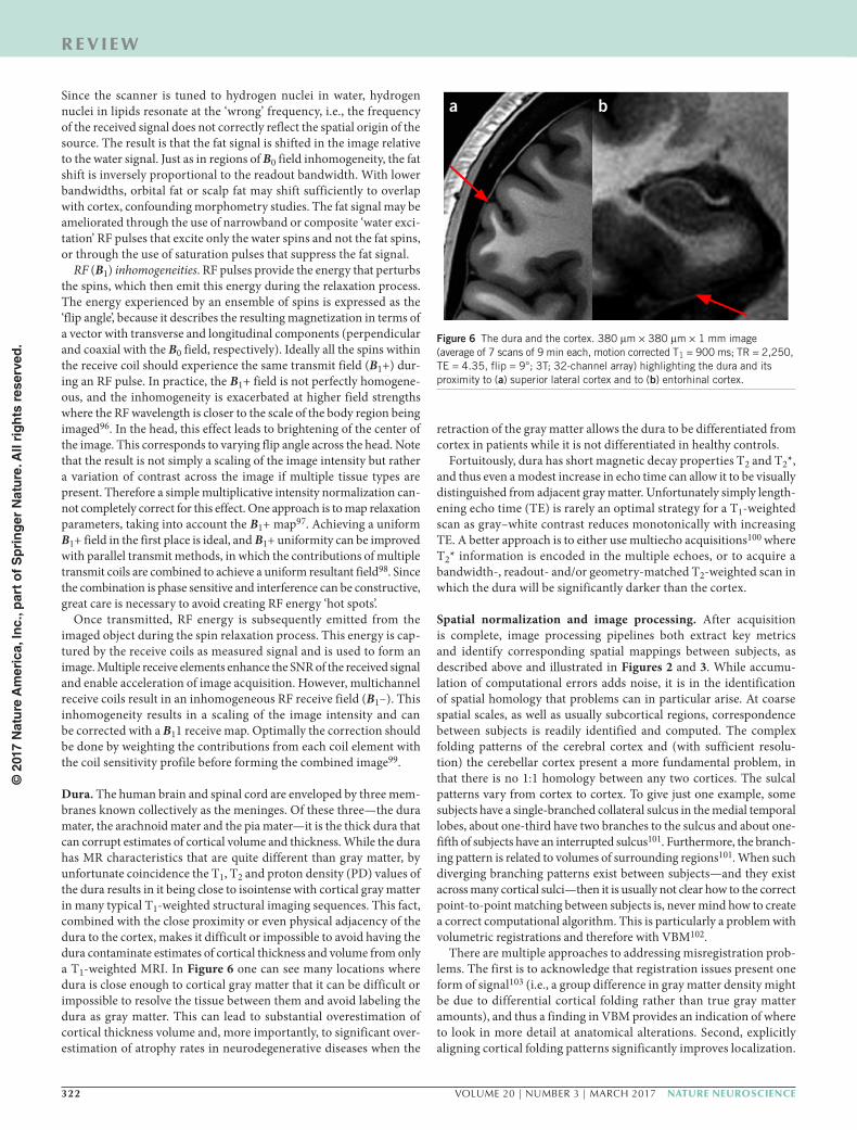
Dura. The human brain and spinal cord are enveloped by three mem-branes known collectively as the meninges. Of these three—the dura mater, the arachnoid mater and the pia mater—it is the thick dura that can corrupt estimates of cortical volume and thickness. While the dura has MR characteristics that are quite different than gray matter, by unfortunate coincidence the T1, T2 and proton density (PD) values of the dura results in it being close to isointense with cortical gray matter in many typical T1-weighted structural imaging sequences. This fact, combined with the close proximity or even physical adjacency of the dura to the cortex, makes it difficult or impossible to avoid having the dura contaminate estimates of cortical thickness and volume from only a T1-weighted MRI. In Figure 6 one can see many locations where dura is close enough to cortical gray matter that it can be difficult or impossible to resolve the tissue between them and avoid labeling the dura as gray matter. This can lead to substantial overestimation of cortical thickness volume and, more importantly, to significant over-estimation of atrophy rates in neurodegenerative diseases when the

retraction of the gray matter allows the dura to be differentiated from cortex in patients while it is not differentiated in healthy controls.

Fortuitously, dura has short magnetic decay properties T2 and T2*, and thus even a modest increase in echo time can allow it to be visually distinguished from adjacent gray matter. Unfortunately simply length-ening echo time (TE) is rarely an optimal strategy for a T1-weighted scan as gray–white contrast reduces monotonically with increasing TE. A better approach is to either use multiecho acquisitions100 where T2* information is encoded in the multiple echoes, or to acquire a bandwidth-, readout- and/or geometry-matched T2-weighted scan in which the dura will be significantly darker than the cortex.

Spatial normalization and image processing. After acquisition is complete, image processing pipelines both extract key metrics and identify corresponding spatial mappings between subjects, as described above and illustrated in Figures 2 and 3. While accumu-lation of computational errors adds noise, it is in the identification of spatial homology that problems can in particular arise. At coarse spatial scales, as well as usually subcortical regions, correspondence between subjects is readily identified and computed. The complex folding patterns of the cerebral cortex and (with sufficient resolu-tion) the cerebellar cortex present a more fundamental problem, in that there is no 1:1 homology between any two cortices. The sulcal patterns vary from cortex to cortex. To give just one example, some subjects have a single-branched collateral sulcus in the medial temporal lobes, about one-third have two branches to the sulcus and about one-fifth of subjects have an interrupted sulcus101. Furthermore, the branch-ing pattern is related to volumes of surrounding regions101. When such diverging branching patterns exist between subjects—and they exist across many cortical sulci—then it is usually not clear how to the correct point-to-point matching between subjects is, never mind how to create a correct computational algorithm. This is particularly a problem with volumetric registrations and therefore with VBM102.

There are multiple approaches to addressing misregistration prob-lems. The first is to acknowledge that registration issues present one form of signal103 (i.e., a group difference in gray matter density might be due to differential cortical folding rather than true gray matter amounts), and thus a finding in VBM provides an indication of where to look in more detail at anatomical alterations. Second, explicitly aligning cortical folding patterns significantly improves localization.

Figure 6 The dura and the cortex. 380 µm × 380 µm × 1 mm image (average of 7 scans of 9 min each, motion corrected T1 = 900 ms; TR = 2,250, TE = 4.35, flip = 9°; 3T; 32-channel array) highlighting the dura and its proximity to (a) superior lateral cortex and to (b) entorhinal cortex.

a b

© 2

017

Nat

ure

Am

eric

a, In

c., p

art

of

Sp

rin

ger

Nat

ure

. All

rig

hts

res

erve

d.

nature neuroscience VOLUME 20 | NUMBER 3 | MARCH 2017 323

r e v i e w

The best illustration for this improvement is in the cross-subject cor-respondence of Broca’s areas (cortical subdivisions based on neuron types and distributions invisible on MRI) after either volumetric or sur-face-based registration, with the surface-based algorithm considerably improving colocalization104. Even surface-based registrations can-not completely account for differential folding patterns (where the true solution is not even known), and thus the third approach is to explicitly map sulcal shapes. The best of known suite of algorithms for sulcal identification and study is in BrainVISA105. Here sizes, loca-tion, branching patterns, etc., can be studied and compared across groups or other metrics of interest. Ultimately, these methods are complementary, and as with acquisition artifacts, understanding the role of possible confounds on final outcomes is key in best advancing science using structural brain imaging.

Structural imaging: current possibilitiesAdvances in ultrahigh field strengths (for example, 7T) offer a route for increased baseline signal (and therefore SNR). This comes at other costs, particular for acquisitions that are affected by shorter T2 relaxa-tion times, worse RF field homogeneity, greater RF power deposition and increased magnetic susceptibility and potential for distortions96. In particular, methods such as diffusion and fast acquisition are chal-lenging to implement robustly at higher field. Nevertheless, establish-ing the right balance between all these factors allows data of very high quality and high spatial resolution106,107. Ultrahigh fields can also have transformative impacts for certain modalities that carry limited information at lower fields. Quantitative susceptibility mapping is an example, with increased contrast at 7T enabling whole-brain quantita-tive susceptibility mapping49 and higher spatial resolution providing iron deposition imaging even in small subcortical nuclei108.

At the same time, multichannel receive coil arrays allow for higher SNR and simultaneous acquisition of more than one slice. The volume extent to be imaged can be separated into a set of equally spaced slices, each driving a high signal in a unique subset of coil elements. The slices can then be acquired simultaneously and the spatial sensitivity of each coil element can be used to separate the signal from different slices. Such simultaneous multislice (or multiband) acquisitions109,110 reduce the time required to scan brain volumes and currently permit 2- to 5-fold acceleration of diffusion MRI scan time111, translating to higher spatial and/or angular resolution and/or SNR per unit time. Multiband acquisitions have been key in improving data qual-ity in different projects (and contexts), such as the adult Human Connectome Project6, UK Biobank5 and the developing Human Connectome Project112.

Modern clinical scanners are equipped with gradient systems that can deliver greater spatial magnetic fields gradients Gmax (~80 mT/m versus 40 mT/m). In diffusion imaging, higher gradient strength leads to greater signal contrast in terms of the signal change for a given displacement of water due to diffusion. In addition, experiments with precise control over the gradient strength and duration (collectively pooled in the parameter q) can permit measurement of small differ-ences in diffusion displacement that may enable estimation of specific microstructural features of tissue. Furthermore, tight head-gradient sets allow fast switching of the gradients (i.e., faster ‘slew rates’) com-pared to whole-body gradient systems. These features collectively allow shorter and stronger gradient pulses for diffusion preparation, which are beneficial in a number of ways, including higher SNR, spatial resolution and angular contrast, and therefore more accurate q-space measurements that technically require infinitely short gradients. Human MR systems have been recently developed with ultrahigh Gmax, such as the Connectome Skyras, which uses 100 and 300 mT/m96,113,

allowing very high data quality114,115. Such hardware capabilities have been very beneficial in mapping microstructure in animals using small-bore systems, and the potential to translate these advantages into in human studies has recently been demonstrated116,117.

The future. Advances in acquisition, image processing and modeling will assuredly keep structural imaging at the forefront of understand-ing brain–behavior relations and how they are altered in development, aging and disease.

A primary focus for diffusion MRI research is in microstructural models that go beyond tensor-derived metrics, such as FA, which are inherently nonspecific. For instance, a reduction in FA has been associated with loss of structure and/or ‘integrity’, while an increase in FA can be indicative of degeneration118. In regions with complex fiber patterns, selective degeneration of one fiber population can lead to an apparent increase in structural coherence; what is left looks macroscopically more ‘organized’.

More complex biophysical models along with sophisticated meas-urements can more precisely explain the measured signal119 and aid interpretation by providing specific markers of microstructure changes120–122. For example, the diffusion signal measured at a range of q-values (gradient areas) exhibits a characteristic diffraction pat-tern in which zero-crossings indicate the size of restricted compart-ments123. Estimation of microscopic features, such as compartment shape and size, using these diffusion measurements have been dem-onstrated on nonbiological model systems using high-performance scanners124. This approach might ultimately enable estimation of mean axon diameters from measurements made perpendicular to a perfectly coherent white matter fiber bundle. In practice, however, such a diffraction pattern cannot be measured with the standard (single-pulse) diffusion sequences or using current hardware avail-able on human scanners. Moreover, these models typically neglect the heterogeneity of fibers within a voxel, which can drive similar sig-nal properties to those of compartmental shape. A recent method125 aims to estimate per-axon diffusivities and anisotropy (microscopic anisotropy), which are inherently free from orientation homogene-ity and heterogeneity assumptions and focus solely on microscopic features of interest. Changing the gradients used for diffusion encod-ing, primarily involving double-diffusion-encoding approaches such as double-pulse diffusion sensitization or oscillating gradients, offer alternative approaches for estimating compartment shape and size, as diffraction measurements of zero-crossings are robust to heter-ogeneities of the imaged system124,126,127. Such sequences are also promising to better characterize restricted diffusion and to probe anisotropy in gray matter voxels or complex crossing white matter bundles (for example128–130; and see Box 1 and Fig. 4). They can even capture diffusional water exchange, a cell membrane permeability-dependent parameter131. While these various methods have demon-strated remarkable potential in model systems, translation into in vivo human imaging remains limited by the hardware and measurement techniques available on human MRI scanners, though this is rapidly improving (for example125,131) and will likely provide exciting break-throughs in the future. These improvements in diffusion imaging techniques will furthermore assist with better tractography, thereby enabling improved localization of the signals origins.

We face an exciting future for the study of neuroanatomy as meth-ods advance, artifacts are understood and their impacts reduced. Our understanding of how the brain changes, be it across development or aging, in response to novel environments or cognitive challenges, or in disease, is still rudimentary. Combining estimates of volumes, thickness, etc. from high-resolution anatomical images with multiple

© 2

017

Nat

ure

Am

eric

a, In

c., p

art

of

Sp

rin

ger

Nat

ure

. All

rig

hts

res

erve

d.

324 VOLUME 20 | NUMBER 3 | MARCH 2017 nature neuroscience

r e v i e w

microstructure modalities, including double-diffusion-encoding approaches, magnetization transfer and susceptibility-weighted imag-ing, and quantitative T1 and T2 mapping, is especially promising. Combining in vivo human imaging with experimental models, with all their genetic and molecular tools, will also provide novel insights. Ultimately, we will come closer and closer to not just mapping what is happening where but to understanding the underlying molecular and cellular bases of our signals.

Also, brain structure provides a common framework to unify multiple neuroscience investigations. Recent years have seen a proliferation of spatially comprehensive and publicly available maps of human brain organization, which are all anatomically grounded but together encompass a vast array of phenotypic dimensions. Salient examples include spatial maps of gene expression (for example, the Allen Brain Atlas, at http://www.brain-map.org/), cytoarchitectonics (http://www.fz-juelich.de/JuBrain/EN/_node.html) and cognitive associations (http://neurosynth.org). The diverse modalities represented by these maps emphasize the fact that structural neuroimaging provides just one of many ways of modeling the brain and also reinforces the fun-damental importance of anatomy as the common spatial framework within which all other phenotypic properties of the brain are embed-ded132. This broad point is well illustrated by several relatively recent studies that use structural neuroimaging data to calculate physical distances between different brain regions and then demonstrate that these distance-based representations of the brain can predict spatial patterns of functional connectivity, metabolism, gene expression and cognitive specialization within the human brain133,134. Thus, the in vivo measures of brain organization provided by structural neuroimaging are not only highly informative and discriminative phenotypes in their own right but also describe the basic anatomical scaffold within which our brains evolve, develop and operate.

AcknowleDgMenTSWe thank C. Hammill for his assistance in the preparation of Figures 2 and 3, which contain data from The Ontario Brain Institutes’ POND grant (to J.P.L.), and we thank L. Wald (Massachusetts General Hospital) for providing the images in Figure 6. Figure 1 contains data from R01MH085772-01A1 (to T.P.).

AUTHoR conTRIBUTIonSJ.P.L., A.J.W.v.d.K., A.R., T.P., H.J.B., K.L.M., S.M.S., B.F. and S.N.S. conceptualized this review. J.P.L., A.J.W.v.d.K., A.R., T.P., B.F. and S.N.S. wrote the initial draft. J.P.L., A.J.W.v.d.K., A.R., T.P., H.J.B., K.L.M., S.M.S., B.F. and S.N.S. edited the final manuscript.

Reprints and permissions information is available online at http://www.nature.com/reprints/index.html.

1. Zilles, K. & Amunts, K. Centenary of Brodmann’s map--conception and fate. Nat. Rev. Neurosci. 11, 139–145 (2010).

2. Gowland, P.A. & Stevenson, V.L. T1: the longitudinal relaxation time. in Quantitative MRI of the Brain (ed. Tofts, P.S.) 111–141 (Wiley, 2003).

3. Bottomley, P.A., Hardy, C.J., Argersinger, R.E. & Allen-Moore, G. A review of 1H nuclear magnetic resonance relaxation in pathology: are T1 and T2 diagnostic? Med. Phys. 14, 1–37 (1987).

4. Boulby, P.A. & Rugg-Gunn, F. T2: the transverse relaxation time. in Quantitative MRI of the Brain (ed. Tofts, P.S.) 143–202 (Wiley, 2003).

5. Miller, K.L. et al. Multimodal population brain imaging in the UK Biobank prospective epidemiological study. Nat. Neurosci. 19, 1523–1536. (2016).

6. Glasser, M.F. et al. The Human Connectome Project’s neuroimaging approach. Nat. Neurosci. 19, 1175–1187 (2016).

7. Chakravarty, M.M. et al. Performing label-fusion-based segmentation using multiple automatically generated templates. Hum. Brain Mapp. 34, 2635–2654 (2013).

8. Ashburner, J. & Friston, K.J. Voxel-based morphometry--the methods. Neuroimage 11, 805–821 (2000).

9. Cao, J. & Worsley, K.J. The detection of local shape changes via the geometry of Hotelling’s T^2 fields. Ann. Stat. 27, 925–942 (1999).

10. Chung, M.K. et al. A unified statistical approach to deformation-based morphometry. Neuroimage 14, 595–606 (2001).

11. Good, C.D. et al. A voxel-based morphometric study of ageing in 465 normal adult human brains. Neuroimage 14, 21–36 (2001).

12. Dale, A.M., Fischl, B. & Sereno, M.I. Cortical surface-based analysis. I. Segmentation and surface reconstruction. Neuroimage 9, 179–194 (1999).

13. Fischl, B., Sereno, M.I. & Dale, A.M. Cortical surface-based analysis. II: inflation, flattening, and a surface-based coordinate system. Neuroimage 9, 195–207 (1999).

14. Kim, J.S. et al. Automated 3-D extraction and evaluation of the inner and outer cortical surfaces using a Laplacian map and partial volume effect classification. Neuroimage 27, 210–221 (2005).

15. Ducharme, S. et al. Trajectories of cortical thickness maturation in normal brain development--The importance of quality control procedures. Neuroimage 125, 267–279 (2016).

16. Amlien, I.K. et al. Organizing principles of human cortical development--thickness and area from 4 to 30 years: insights from comparative primate neuroanatomy. Cereb. Cortex 26, 257–267 (2016).

17. Raznahan, A. et al. Globally divergent but locally convergent X- and Y-chromosome influences on cortical development. Cereb. Cortex 26, 70–79 (2016).

18. Chen, C.-H. et al. Genetic topography of brain morphology. Proc. Natl. Acad. Sci. USA 110, 17089–17094 (2013).

19. Raznahan, A., Greenstein, D., Lee, N.R., Clasen, L.S. & Giedd, J.N. Prenatal growth in humans and postnatal brain maturation into late adolescence. Proc. Natl. Acad. Sci. USA 109, 11366–11371 (2012).

20. Schmaal, L. et al. Cortical abnormalities in adults and adolescents with major depression based on brain scans from 20 cohorts worldwide in the ENIGMA Major Depressive Disorder Working Group. Mol. Psychiatry http://dx.doi.org/10.1038/mp.2016.60 (2016).

21. Smith, E. et al. Cortical thickness change in autism during early childhood. Hum. Brain Mapp. 37, 2616–2629 (2016).

22. Lerch, J.P. & Evans, A.C. Cortical thickness analysis examined through power analysis and a population simulation. Neuroimage 24, 163–173 (2005).

23. Jbabdi, S., Sotiropoulos, S.N., Haber, S.N., Van Essen, D.C. & Behrens, T.E. Measuring macroscopic brain connections in vivo. Nat. Neurosci. 18, 1546–1555 (2015).

24. Tardif, C.L., Collins, D.L. & Pike, G.B. Sensitivity of voxel-based morphometry analysis to choice of imaging protocol at 3 T. Neuroimage 44, 827–838 (2009).

25. Tardif, C.L., Collins, D.L. & Pike, G.B. Regional impact of field strength on voxel-based morphometry results. Hum. Brain Mapp. 31, 943–957 (2010).

26. Lüsebrink, F., Wollrab, A. & Speck, O. Cortical thickness determination of the human brain using high resolution 3T and 7T MRI data. Neuroimage 70, 122–131 (2013).

27. Scholtens, L.H., de Reus, M.A. & van den Heuvel, M.P. Linking contemporary high resolution magnetic resonance imaging to the von Economo legacy: A study on the comparison of MRI cortical thickness and histological measurements of cortical structure. Hum. Brain Mapp. 36, 3038–3046 (2015).

28. Basser, P.J., Mattiello, J. & LeBihan, D. MR diffusion tensor spectroscopy and imaging. Biophys. J. 66, 259–267 (1994).

29. Pierpaoli, C. & Basser, P.J. Toward a quantitative assessment of diffusion anisotropy. Magn. Reson. Med. 36, 893–906 (1996).

30. Simon, T.J. et al. Volumetric, connective, and morphologic changes in the brains of children with chromosome 22q11.2 deletion syndrome: an integrative study. Neuroimage 25, 169–180 (2005).

31. Voineskos, A.N. et al. Quantitative examination of a novel clustering method using magnetic resonance diffusion tensor tractography. Neuroimage 45, 370–376 (2009).

32. Smith, S.M. et al. Tract-based spatial statistics: voxelwise analysis of multi-subject diffusion data. Neuroimage 31, 1487–1505 (2006).

33. Yushkevich, P.A., Zhang, H., Simon, T.J. & Gee, J.C. Structure-specific statistical mapping of white matter tracts. Neuroimage 41, 448–461 (2008).

34. Jensen, J.H. & Helpern, J.A. MRI quantification of non-Gaussian water diffusion by kurtosis analysis. NMR Biomed. 23, 698–710 (2010).

35. Fieremans, E., Jensen, J.H. & Helpern, J.A. White matter characterization with diffusional kurtosis imaging. Neuroimage 58, 177–188 (2011).

36. McGowan, J.C. The physical basis of magnetization transfer imaging. Neurology 53 (Suppl. 3), S3–S7 (1999).

37. Kucharczyk, W., Macdonald, P.M., Stanisz, G.J. & Henkelman, R.M. Relaxivity and magnetization transfer of white matter lipids at MR imaging: importance of cerebrosides and pH. Radiology 192, 521–529 (1994).

38. Laule, C. et al. Magnetic resonance imaging of myelin. Neurotherapeutics 4, 460–484 (2007).

39. Pike, G.B. Pulsed magnetization transfer contrast in gradient echo imaging: a two-pool analytic description of signal response. Magn. Reson. Med. 36, 95–103 (1996).

40. Ward, K.M., Aletras, A.H. & Balaban, R.S. A new class of contrast agents for MRI based on proton chemical exchange dependent saturation transfer (CEST). J. Magn. Reson. 143, 79–87 (2000).

41. Tee, Y.K. et al. Comparing different analysis methods for quantifying the MRI amide proton transfer (APT) effect in hyperacute stroke patients. NMR Biomed. 27, 1019–1029 (2014).

42. Walker-Samuel, S. et al. In vivo imaging of glucose uptake and metabolism in tumors. Nat. Med. 19, 1067–1072 (2013).

43. Tardif, C.L. et al. Advanced MRI techniques to improve our understanding of experience-induced neuroplasticity. Neuroimage 131, 55–72 (2016).

44. Mugler, J.P., III & Brookeman, J.R. Three-dimensional magnetization-prepared rapid gradient-echo imaging (3D MP RAGE). Magn. Reson. Med. 15, 152–157 (1990).

© 2

017

Nat

ure

Am

eric

a, In

c., p

art

of

Sp

rin

ger

Nat

ure

. All

rig

hts

res

erve

d.

nature neuroscience VOLUME 20 | NUMBER 3 | MARCH 2017 325

r e v i e w

45. Deoni, S.C.L., Peters, T.M. & Rutt, B.K. High-resolution T1 and T2 mapping of the brain in a clinically acceptable time with DESPOT1 and DESPOT2. Magn. Reson. Med. 53, 237–241 (2005).

46. Fram, E.K. et al. Rapid calculation of T1 using variable flip angle gradient refocused imaging. Magn. Reson. Imaging 5, 201–208 (1987).

47. Preibisch, C. & Deichmann, R. T1 mapping using spoiled FLASH-EPI hybrid sequences and varying flip angles. Magn. Reson. Med. 62, 240–246 (2009).

48. Stikov, N. et al. On the accuracy of T1 mapping: searching for common ground. Magn. Reson. Med. 73, 514–522 (2015).

49. Shmueli, K. et al. Magnetic susceptibility mapping of brain tissue in vivo using MRI phase data. Magn. Reson. Med. 62, 1510–1522 (2009).

50. Mechelli, A., Friston, K.J., Frackowiak, R.S. & Price, C.J. Structural covariance in the human cortex. J. Neurosci. 25, 8303–8310 (2005).

51. Lerch, J.P. et al. Mapping anatomical correlations across cerebral cortex (MACACC) using cortical thickness from MRI. Neuroimage 31, 993–1003 (2006).

52. Alexander-Bloch, A., Giedd, J.N. & Bullmore, E. Imaging structural co-variance between human brain regions. Nat. Rev. Neurosci. 14, 322–336 (2013).

53. Evans, A.C. Networks of anatomical covariance. Neuroimage 80, 489–504 (2013).

54. Reid, A.T. et al. A seed-based cross-modal comparison of brain connectivity measures. Brain Struct. Funct. (2016).

55. Maguire, E.A. et al. Navigation-related structural change in the hippocampi of taxi drivers. Proc. Natl. Acad. Sci. USA 97, 4398–4403 (2000).

56. Draganski, B. et al. Neuroplasticity: changes in grey matter induced by training. Nature 427, 311–312 (2004).

57. Driemeyer, J., Boyke, J., Gaser, C., Büchel, C. & May, A. Changes in gray matter induced by learning--revisited. PLoS One 3, e2669 (2008).

58. Scholz, J., Klein, M.C., Behrens, T.E.J. & Johansen-Berg, H. Training induces changes in white-matter architecture. Nat. Neurosci. 12, 1370–1371 (2009).

59. Sagi, Y. et al. Learning in the fast lane: new insights into neuroplasticity. Neuron 73, 1195–1203 (2012).

60. Taubert, M. et al. Dynamic properties of human brain structure: learning-related changes in cortical areas and associated fiber connections. J. Neurosci. 30, 11670–11677 (2010).

61. Hyde, K.L. et al. Musical training shapes structural brain development. J. Neurosci. 29, 3019–3025 (2009).

62. Bengtsson, S.L. et al. Extensive piano practicing has regionally specific effects on white matter development. Nat. Neurosci. 8, 1148–1150 (2005).

63. Thomas, C. & Baker, C.I. Teaching an adult brain new tricks: a critical review of evidence for training-dependent structural plasticity in humans. Neuroimage 73, 225–236 (2013).

64. Thomas, A.G. et al. Functional but not structural changes associated with learning: an exploration of longitudinal voxel-based morphometry (VBM). Neuroimage 48, 117–125 (2009).

65. Lerch, J.P. et al. Maze training in mice induces MRI-detectable brain shape changes specific to the type of learning. Neuroimage 54, 2086–2095 (2011).

66. Blumenfeld-Katzir, T., Pasternak, O., Dagan, M. & Assaf, Y. Diffusion MRI of structural brain plasticity induced by a learning and memory task. PLoS One 6, e20678 (2011).

67. Scholz, J., Allemang-Grand, R., Dazai, J. & Lerch, J.P. Environmental enrichment is associated with rapid volumetric brain changes in adult mice. Neuroimage 109, 190–198 (2015).

68. Sampaio-Baptista, C. et al. Motor skill learning induces changes in white matter microstructure and myelination. J. Neurosci. 33, 19499–19503 (2013).

69. Golub, Y. et al. Reduced hippocampus volume in the mouse model of Posttraumatic Stress Disorder. J. Psychiatric Res. 45, 650–659 (2011).

70. Keifer, O.P. Jr. et al. Voxel-based morphometry predicts shifts in dendritic spine density and morphology with auditory fear conditioning. Nat Commun 6, 7582 (2015).

71. Biedermann, S. et al. In vivo voxel based morphometry: detection of increased hippocampal volume and decreased glutamate levels in exercising mice. Neuroimage 61, 1206–1212 (2012).

72. Fuss, J. et al. Exercise boosts hippocampal volume by preventing early age-related gray matter loss. Hippocampus 24, 131–134 (2014).

73. Jespersen, S.N. et al. Neurite density from magnetic resonance diffusion measurements at ultrahigh field: comparison with light microscopy and electron microscopy. Neuroimage 49, 205–216 (2010).

74. Sepehrband, F. et al. Brain tissue compartment density estimated using diffusion-weighted MRI yields tissue parameters consistent with histology. Hum. Brain Mapp. 36, 3687–3702 (2015).

75. Stikov, N. et al. In vivo histology of the myelin g-ratio with magnetic resonance imaging. Neuroimage 118, 397–405 (2015).

76. Jones, D.K., Knösche, T.R. & Turner, R. White matter integrity, fiber count, and other fallacies: the do’s and don’ts of diffusion MRI. Neuroimage 73, 239–254 (2013).

77. Streitbürger, D.-P. et al. Investigating structural brain changes of dehydration using voxel-based morphometry. PLoS One 7, e44195 (2012).

78. Trefler, A. et al. Impact of time-of-day on brain morphometric measures derived from T1-weighted magnetic resonance imaging. Neuroimage 133, 41–52 (2016).

79. Satterthwaite, T.D. et al. Impact of in-scanner head motion on multiple measures of functional connectivity: relevance for studies of neurodevelopment in youth. Neuroimage 60, 623–632 (2012).

80. Reuter, M. et al. Head motion during MRI acquisition reduces gray matter volume and thickness estimates. Neuroimage 107, 107–115 (2015).

81. Alexander-Bloch, A. et al. Subtle in-scanner motion biases automated measurement of brain anatomy from in vivo MRI. Hum. Brain Mapp. 37, 2385–2397 (2016).

82. Yendiki, A., Koldewyn, K., Kakunoori, S., Kanwisher, N. & Fischl, B. Spurious group differences due to head motion in a diffusion MRI study. Neuroimage 88, 79–90 (2014).

83. Pardoe, H.R., Kucharsky Hiess, R. & Kuzniecky, R. Motion and morphometry in clinical and nonclinical populations. Neuroimage 135, 177–185 (2016).

84. Andersson, J.L.R. & Sotiropoulos, S.N. An integrated approach to correction for off-resonance effects and subject movement in diffusion MR imaging. Neuroimage 125, 1063–1078 (2016).

85. Chang, L.-C., Walker, L. & Pierpaoli, C. Informed RESTORE: A method for robust estimation of diffusion tensor from low redundancy datasets in the presence of physiological noise artifacts. Magn. Reson. Med. 68, 1654–1663 (2012).

86. Andersson, J.L.R., Graham, M.S., Zsoldos, E. & Sotiropoulos, S.N. Incorporating outlier detection and replacement into a non-parametric framework for movement and distortion correction of diffusion MR images. Neuroimage 141, 556–572 (2016).

87. Thesen, S., Heid, O., Mueller, E. & Schad, L.R. Prospective acquisition correction for head motion with image-based tracking for real-time fMRI. Magn. Reson. Med. 44, 457–465 (2000).

88. van der Kouwe, A., Fetics, B., Polenur, D., Roth, A. & Nevo, E. Real-time prospective rigid-body motion correction with the EndoScout gradient-based tracking system. in Proc. 17th Scientific Meeting ISMRM 17, 4623, (2009).

89. Ooi, M.B. et al. Combined prospective and retrospective correction to reduce motion-induced image misalignment and geometric distortions in EPI. Magn. Reson. Med. 69, 803–811 (2013).

90. van Niekerk, A.M.J. et al. O51. A vector based approach for fast real time orientation measurement in magnetic resonance imaging (MRI). Phys. Med. 32, 158 (2016).

91. Olesen, O.V., Paulsen, R.R., Højgaard, L., Roed, B. & Larsen, R. Motion tracking for medical imaging: a nonvisible structured light tracking approach. IEEE Trans. Med. Imaging 31, 79–87 (2012).

92. van der Kouwe, A.J.W., Benner, T. & Dale, A.M. Real-time rigid body motion correction and shimming using cloverleaf navigators. Magn. Reson. Med. 56, 1019–1032 (2006).

93. Gallichan, D., Marques, J.P. & Gruetter, R. Retrospective correction of involuntary microscopic head movement using highly accelerated fat image navigators (3D FatNavs) at 7T. Magn. Reson. Med. 75, 1030–1039 (2016).

94. Tisdall, M.D. et al. Prospective motion correction with volumetric navigators (vNavs) reduces the bias and variance in brain morphometry induced by subject motion. Neuroimage 127, 11–22 (2016).

95. Glasser, M.F. et al. The minimal preprocessing pipelines for the Human Connectome Project. Neuroimage 80, 105–124 (2013).

96. Ugurbil, K. et al. Pushing spatial and temporal resolution for functional and diffusion MRI in the Human Connectome Project. Neuroimage 80, 80–104 (2013).

97. Deoni, S.C.L. Correction of main and transmit magnetic field (B0 and B1) inhomogeneity effects in multicomponent-driven equilibrium single-pulse observation of T1 and T2. Magn. Reson. Med. 65, 1021–1035 (2011).

98. Umesh Rudrapatna, S., Juchem, C., Nixon, T.W. & de Graaf, R.A. Dynamic multi-coil tailored excitation for transmit B1 correction at 7 Tesla. Magn. Reson. Med. 76, 83–93 (2016).

99. Watanabe, H., Takaya, N. & Mitsumori, F. Non-uniformity correction of human brain imaging at high field by RF field mapping of B1+ and B1−. J. Magn. Reson. 212, 426–430 (2011).

100. van der Kouwe, A.J.W., Benner, T., Salat, D.H. & Fischl, B. Brain morphometry with multiecho MPRAGE. Neuroimage 40, 559–569 (2008).

101. Pruessner, J.C. et al. Volumetry of temporopolar, perirhinal, entorhinal and parahippocampal cortex from high-resolution MR images: considering the variability of the collateral sulcus. Cereb. Cortex 12, 1342–1353 (2002).

102. Bookstein, F.L. “Voxel-based morphometry” should not be used with imperfectly registered images. Neuroimage 14, 1454–1462 (2001).

103. Ashburner, J. & Friston, K.J. Why voxel-based morphometry should be used. Neuroimage 14, 1238–1243 (2001).

104. Fischl, B. et al. Cortical folding patterns and predicting cytoarchitecture. Cereb. Cortex 18, 1973–1980 (2008).

105. Mangin, J.-F. et al. A framework to study the cortical folding patterns. Neuroimage 23 (Suppl. 1), S129–S138 (2004).

106. Eichner, C. et al. Slice accelerated diffusion-weighted imaging at ultra-high field strength. Magn. Reson. Med. 71, 1518–1525 (2014).

107. Vu, A.T. et al. High resolution whole brain diffusion imaging at 7T for the Human Connectome Project. Neuroimage 122, 318–331 (2015).

108. Schäfer, A. et al. Direct visualization of the subthalamic nucleus and its iron distribution using high-resolution susceptibility mapping. Hum. Brain Mapp. 33, 2831–2842 (2012).

109. Setsompop, K. et al. Blipped-controlled aliasing in parallel imaging for simultaneous multislice echo planar imaging with reduced g-factor penalty. Magn. Reson. Med. 67, 1210–1224 (2012).

110. Moeller, S. et al. Multiband multislice GE-EPI at 7 tesla, with 16-fold acceleration using partial parallel imaging with application to high spatial and temporal whole-brain fMRI. Magn. Reson. Med. 63, 1144–1153 (2010).

© 2

017

Nat

ure

Am

eric

a, In

c., p

art

of

Sp

rin

ger

Nat

ure

. All

rig

hts

res

erve

d.

326 VOLUME 20 | NUMBER 3 | MARCH 2017 nature neuroscience

r e v i e w

111. Xu, J. et al. Evaluation of slice accelerations using multiband echo planar imaging at 3 T. Neuroimage 83, 991–1001 (2013).

112. Hughes, E.J. et al. A dedicated neonatal brain imaging system. Magn. Reson. Med. http://dx.doi.org/10.1002/mrm.26462 (2016).

113. Setsompop, K. et al. Pushing the limits of in vivo diffusion MRI for the Human Connectome Project. Neuroimage 80, 220–233 (2013).

114. Sotiropoulos, S.N. et al. Advances in diffusion MRI acquisition and processing in the Human Connectome Project. Neuroimage 80, 125–143 (2013).

115. Fan, Q. et al. MGH-USC Human Connectome Project datasets with ultra-high b-value diffusion MRI. Neuroimage 124 (Pt. B), 1108–1114 (2016).

116. McNab, J.A. et al. The Human Connectome Project and beyond: initial applications of 300 mT/m gradients. Neuroimage 80, 234–245 (2013).

117. Ferizi, U. et al. White matter compartment models for in vivo diffusion MRI at 300mT/m. Neuroimage 118, 468–483 (2015).

118. Douaud, G. et al. In vivo evidence for the selective subcortical degeneration in Huntington’s disease. Neuroimage 46, 958–966 (2009).

119. Panagiotaki, E. et al. Compartment models of the diffusion MR signal in brain white matter: a taxonomy and comparison. Neuroimage 59, 2241–2254 (2012).

120. Jelescu, I.O. et al. In vivo quantification of demyelination and recovery using compartment-specific diffusion MRI metrics validated by electron microscopy. Neuroimage 132, 104–114 (2016).

121. Kodiweera, C., Alexander, A.L., Harezlak, J., McAllister, T.W. & Wu, Y.-C. Age effects and sex differences in human brain white matter of young to middle-aged adults: A DTI, NODDI, and q-space study. Neuroimage 128, 180–192 (2016).

122. Colgan, N. et al. Application of neurite orientation dispersion and density imaging (NODDI) to a tau pathology model of Alzheimer’s disease. Neuroimage 125, 739–744 (2016).

123. Callaghan, P.T., Coy, A., MacGowan, D., Packer, K.J. & Zelaya, F.O. Diffraction-like effects in NMR diffusion studies of fluids in porous solids. Nature 351, 467–469 (1991).

124. Shemesh, N., Ozarslan, E., Komlosh, M.E., Basser, P.J. & Cohen, Y. From single-pulsed field gradient to double-pulsed field gradient MR: gleaning new microstructural information and developing new forms of contrast in MRI. NMR Biomed. 23, 757–780 (2010).

125. Kaden, E., Kruggel, F. & Alexander, D.C. Quantitative mapping of the per-axon diffusion coefficients in brain white matter. Magn. Reson. Med. 75, 1752–1763 (2016).

126. Ozarslan, E. Compartment shape anisotropy (CSA) revealed by double pulsed field gradient MR. J. Magn. Reson. 199, 56–67 (2009).

127. Drobnjak, I., Zhang, H., Ianus, A., Kaden, E. & Alexander, D.C. PGSE, OGSE, and sensitivity to axon diameter in diffusion MRI: Insight from a simulation study. Magn. Reson. Med. 75, 688–700 (2016).

128. Nilsson, M., van Westen, D., Ståhlberg, F., Sundgren, P.C. & Lätt, J. The role of tissue microstructure and water exchange in biophysical modeling of diffusion in white matter. MAGMA 26, 345–370 (2013).

129. Westin, C.-F. et al. Q-space trajectory imaging for multidimensional diffusion MRI of the human brain. Neuroimage 135, 345–362 (2016).

130. Reisert, M., Kellner, E., Dhital, B., Hennig, J. & Kiselev, V.G. Disentangling micro from mesostructure by diffusion MRI: A Bayesian approach. Neuroimage S1053-8119(16)30535-3 http://dx.doi.org/10.1016/j.neuroimage.2016.09.058 (2016).

131. Lampinen, B. et al. Optimal experimental design for filter exchange imaging: Apparent exchange rate measurements in the healthy brain and in intracranial tumors. Magn. Reson. Med. http://dx.doi.org/10.1002/mrm.26195 (2016).

132. Devlin, J.T. & Poldrack, R.A. In praise of tedious anatomy. Neuroimage 37, 1033–1041, discussion 1050–1058 (2007).

133. Margulies, D.S. et al. Situating the default-mode network along a principal gradient of macroscale cortical organization. Proc. Natl. Acad. Sci. USA 113, 12574–12579 (2016).

134. Collin, G., Sporns, O., Mandl, R.C.W. & van den Heuvel, M.P. Structural and functional aspects relating to cost and benefit of rich club organization in the human cerebral cortex. Cereb. Cortex 24, 2258–2267 (2014).

135. Assaf, Y. & Cohen, Y. Non-mono-exponential attenuation of water and N-acetyl aspartate signals due to diffusion in brain tissue. J. Magn. Reson. 131, 69–85 (1998).

136. Clark, C.A. & Le Bihan, D. Water diffusion compartmentation and anisotropy at high b values in the human brain. Magn. Reson. Med. 44, 852–859 (2000).

137. Stanisz, G.J., Szafer, A., Wright, G.A. & Henkelman, R.M. An analytical model of restricted diffusion in bovine optic nerve. Magn. Reson. Med. 37, 103–111 (1997).

138. Behrens, T.E. et al. Characterization and propagation of uncertainty in diffusion-weighted MR imaging. Magn. Reson. Med. 50, 1077–1088 (2003).

139. Assaf, Y. & Basser, P.J. Composite hindered and restricted model of diffusion (CHARMED) MR imaging of the human brain. Neuroimage 27, 48–58 (2005).

140. Assaf, Y., Blumenfeld-Katzir, T., Yovel, Y. & Basser, P.J. AxCaliber: a method for measuring axon diameter distribution from diffusion MRI. Magn. Reson. Med. 59, 1347–1354 (2008).

141. Barazany, D., Basser, P.J. & Assaf, Y. In vivo measurement of axon diameter distribution in the corpus callosum of rat brain. Brain 132, 1210–1220 (2009).

142. Alexander, D.C. et al. Orientationally invariant indices of axon diameter and density from diffusion MRI. Neuroimage 52, 1374–1389 (2010).

143. Tournier, J.-D., Mori, S. & Leemans, A. Diffusion tensor imaging and beyond. Magn. Reson. Med. 65, 1532–1556 (2011).

144. Dell’Acqua, F., Simmons, A., Williams, S.C.R. & Catani, M. Can spherical deconvolution provide more information than fiber orientations? Hindrance modulated orientational anisotropy, a true-tract specific index to characterize white matter diffusion. Hum. Brain Mapp. 34, 2464–2483 (2013).

145. Kaden, E., Knösche, T.R. & Anwander, A. Parametric spherical deconvolution: inferring anatomical connectivity using diffusion MR imaging. Neuroimage 37, 474–488 (2007).

146. Sotiropoulos, S.N., Behrens, T.E.J. & Jbabdi, S. Ball and rackets: Inferring fiber fanning from diffusion-weighted MRI. Neuroimage 60, 1412–1425 (2012).

147. Zhang, H., Schneider, T., Wheeler-Kingshott, C.A. & Alexander, D.C. NODDI: practical in vivo neurite orientation dispersion and density imaging of the human brain. Neuroimage 61, 1000–1016 (2012).

148. Paus, T. Population Neuroscience. (Springer-Verlag, 2013).149. Falk, E.B. et al. What is a representative brain? Neuroscience meets population

science. Proc. Natl. Acad. Sci. USA 110, 17615–17622 (2013).150. Paus, T. Population neuroscience. in Neuroepidemiology, Volume 138 (eds.

Rosano, C.I.M., Ikram, M.A. & Ganguli, M.) 17–37 (Elsevier, 2016).151. Alzheimer’s Disease Neuroimaging Initiative, EPIGEN Consortium, IMAGEN

Consortium, Saguenay Youth Study (SYS) Group. The ENIGMA Consortium: large-scale collaborative analyses of neuroimaging and genetic data. Brain Imaging Behav. 8, 153–182 (2014).

152. CHARGE Consortium. Design of prospective meta-analyses of genome-wide association studies from 5 cohorts. Circ Cardiovasc Genet 2, 73–80 (2009).

153. Odgers, C.L., Caspi, A., Bates, C.J., Sampson, R.J. & Moffitt, T.E. Systematic social observation of children’s neighborhoods using Google Street View: a reliable and cost-effective method. J. Child Psychol. Psychiatry 53, 1009–1017 (2012).

154. Mazziotta, J. et al. A probabilistic atlas and reference system for the human brain: International Consortium for Brain Mapping (ICBM). Phil. Trans. R. Soc. Lond. B 356, 1293–1322 (2001).

155. French, L. & Paus, T. A FreeSurfer view of the cortical transcriptome generated from the Allen Human Brain Atlas. Front. Neurosci. 9, 323 (2015).

156. French, L. et al. early cannabis use, polygenic risk score for schizophrenia and brain maturation in adolescence. JAMA Psychiatry 72, 1002–1011 (2015).

157. Giedd, J.N. et al. Brain development during childhood and adolescence: a longitudinal MRI study. Nat. Neurosci. 2, 861–863 (1999).

158. Mills, K.L. et al. Structural brain development between childhood and adulthood: Convergence across four longitudinal samples. Neuroimage 141, 273–281 (2016).

159. Raznahan, A. et al. Longitudinal four-dimensional mapping of subcortical anatomy in human development. Proc. Natl. Acad. Sci. USA 111, 1592–1597 (2014).

160. Schmitt, J.E. et al. The dynamic role of genetics on cortical patterning during childhood and adolescence. Proc. Natl. Acad. Sci. USA 111, 6774–6779 (2014).

161. Shaw, P. et al. Intellectual ability and cortical development in children and adolescents. Nature 440, 676–679 (2006).

162. Shaw, P. et al. Attention-deficit/hyperactivity disorder is characterized by a delay in cortical maturation. Proc. Natl. Acad. Sci. USA 104, 19649–19654 (2007).

163. Raznahan, A. et al. Patterns of coordinated anatomical change in human cortical development: a longitudinal neuroimaging study of maturational coupling. Neuron 72, 873–884 (2011).

164. Vandekar, S.N. et al. Topologically dissociable patterns of development of the human cerebral cortex. J. Neurosci. 35, 599–609 (2015).

165. Toro, R. et al. Brain volumes and Val66Met polymorphism of the BDNF gene: local or global effects? Brain Struct. Funct. 213, 501–509 (2009).

166. Reardon, P.K. et al. An Allometric Analysis of Sex and Sex Chromosome Dosage Effects on Subcortical Anatomy in Humans. J. Neurosci. 36, 2438–2448 (2016).

167. Lee, N.R. et al. Anatomical coupling among distributed cortical regions in youth varies as a function of individual differences in vocabulary abilities. Hum. Brain Mapp. 35, 1885–1895 (2014).

168. Alexander-Bloch, A.F. et al. Abnormal cortical growth in schizophrenia targets normative modules of synchronized development. Biol. Psychiatry 76, 438–446 (2014).

169. Honey, C.J. et al. Predicting human resting-state functional connectivity from structural connectivity. Proc. Natl. Acad. Sci. USA 106, 2035–2040 (2009).

170. Alexander-Bloch, A., Raznahan, A., Bullmore, E. & Giedd, J. The convergence of maturational change and structural covariance in human cortical networks. J. Neurosci. 33, 2889–2899 (2013).

171. Seeley, W.W., Crawford, R.K., Zhou, J., Miller, B.L. & Greicius, M.D. Neurodegenerative diseases target large-scale human brain networks. Neuron 62, 42–52 (2009).

172. Studholme, C. Mapping fetal brain development in utero using magnetic resonance imaging: the Big Bang of brain mapping. Annu. Rev. Biomed. Eng. 13, 345–368 (2011).

173. Kim, H. et al. NEOCIVET: Towards accurate morphometry of neonatal gyrification and clinical applications in preterm newborns. Neuroimage 138, 28–42 (2016).

174. Dubois, J. et al. Primary cortical folding in the human newborn: an early marker of later functional development. Brain 131, 2028–2041 (2008).

175. Anderson, P.J., Cheong, J.L.Y. & Thompson, D.K. The predictive validity of neonatal MRI for neurodevelopmental outcome in very preterm children. Semin. Perinatol. 39, 147–158 (2015).

© 2

017

Nat

ure

Am

eric

a, In

c., p

art

of

Sp

rin

ger

Nat

ure

. All

rig

hts

res

erve

d.