studies on the characteristics oftropical...

Chapter 1

Introduction

Chapter # 1 Introduction

1.1. Vertical Structure of the Atmosphere

Temperature varies greatly both vertically and horizontally as well as temporally

throughout the atmosphere. However, despite horizontal variations, the vertical structure

of temperature characterizes the Earth’s atmospheric layers. These variations in

temperature are produced by differences in the radiation budget and chemical

composition of the atmosphere at different altitudes. Based on temperature changes with

altitude, the Earth’s atmosphere is divided into mainly four concentric spherical shells,

namely, troposphere, stratosphere, mesosphere, and thermosphere. The vertical

distribution of temperature in the Earth’s atmosphere is shown in Figure 1.1.

The Troposphere: Troposphere is the lowest part of the Earth’s atmosphere whose

thickness decreases from equator to pole, and is higher in summer than in winter. It

extends ~16-18 km at tropics, 10-12 km at mid latitude and 6-8 km at polar region. The

greater thickness of the troposphere over the tropics is due to greater solar radiation. The

solar radiation heats the surface and the air is warmed by sensible and latent heat fluxes.

The warmed surface air which rises aloft to higher altitudes owing to lower density

increases the thickness of the troposphere over tropics. The troposphere holds almost

~80% (~90% in the tropics) of the mass of the earth’s atmosphere and nearly all the water

vapor (~99%). The water vapor raises aloft get condense and then precipitate with release

of latent heat which drives the atmospheric phenomena. The density and pressure

decreases exponentially with altitude. In the troposphere, temperature decreases linearly

with a lapse rate of 6-7 K/km. It may be noted that the tropospheric gases are mostly

transparent to the incoming solar radiation which allow it to heat the earth surface. The

earth’s surface emits long wave radiation which is absorbed and reradiated by the

tropospheric gases.

The troposphere is well mixed and highly unstable due to differential heating owing

to large land-sea contrasts which are important for monsoonal circulations. However, the

latitudinal differential heating is responsible for midlatitude weather systems. The lower

troposphere attains convective equilibrium due to release of latent heat during cloud

formation and precipitation. Like pressure and density, temperature doesn’t decrease

continuously but start to increase above troposphere in the stratosphere due to presence of

ozone layer, which absorbs almost all the ultra violet (UV) part of the solar radiation. The

1


boundary which separates troposphere and stratosphere is known as tropopause. In this

layer temperature is relatively constant (not always, very sharp changes may also occur)

with altitude. The tropopause is not a continuous layer, but there are breaks, between

midlatitudes and polar tropopause associated with polar front jet streams, and the

midlatitude and tropical tropopause associated with subtropical jet streams. The

tropopause acts as a lid which resists the exchange of air between troposphere and

stratosphere. However, due to greater convection most of the upward exchange of the air

takes place through tropical tropopause region. The tropical tropopause and its

importance will be discussed in detail in later sections.

Figure1.1: Mean vertical thermal structure of Earth’s atmosphere. [Adapted from G. Brasseur and S.

Solomon 1984].

2


The Stratosphere: The stratosphere is characterized by high stability and very long

vertical mixing time scale in contrast to troposphere. The most significant minor

constituent of the stratosphere is ozone which is found maximum at altitude ~ 20-30 km.

As mentioned earlier the UV (0.1 µm to 0.35 µm) part of the solar radiation is observed

by this layer, which plays the major role in regulating the thermal regime of this layer.

The reason for the existence of ozone at these levels is that it is produced here, as a by-

product of the photo-dissociation (photolysis) of molecular oxygen, producing atomic

oxygen which then combines with molecular oxygen thus:

O2 + hν → O + O ,

O + O2 + M → O3 + M

where hν is the energy of incoming photons (ν is their frequency and h is Planck’s

constant) and M is any third body. Ozone absorbs UV radiation and with the low

densities present at stratospheric altitudes, this absorption is an efficient mechanism of

transferring kinetic energy to a relatively small number of molecules causing increase of

the temperature from the tropopause to an altitude ~ 50 km. Thus, the –ve lapse rate (~

3K/km) doesn’t allow rapid mixing between the stable layers. The mixing in lower

stratosphere takes place in time scale of a month or year. The resulting ozone, through its

radiative properties, is the reason for the existence of the stratosphere. It is close to

radiative equilibrium. The boundary which separates the stratosphere and mesosphere is

known as stratopause, which occurs at an altitude of 45–55 km, the level at which

temperature ceases to increase with altitude. The temperature of the stratopause varies in

the range 240 K to 290 K over winter pole to summer pole.

The Mesosphere: In contrast to the stratosphere, mesosphere is highly unstable, like

troposphere, with rapid mixing through convective currents. The mesosphere is

dominated by molecular oxygen (O2) and carbon dioxide (CO2). The radiative heating of

molecular oxygen and radiative cooling by infrared emission of carbon dioxide determine

the heat balance in this region. The temperature decreases rapidly from stratopause to

altitude ~80-90 km. Compared to lower regions, the concentrations of ozone and water

vapor in the mesosphere are negligible, hence the lower temperatures. Its chemical

composition is fairly uniform. Pressures are very low. The mesopause, which separates

the thermosphere and mesosphere, is coldest region in the Earth’s atmosphere whose

3


temperature is ~ 180 K at altitude ~ 80 km -100 km. Extreme low mesopause temperature

occur during Northern Hemispheric Summer. At the end of above these altitudes, the

atmosphere becomes ionized (the ionosphere), causing reflection of radio waves, a

property of the upper atmosphere which is of great practical importance. The

Thermosphere is the region of high temperatures above the mesosphere. It includes the

ionosphere and extends out to several hundred kilometers. It is here that very short

wavelength UV is absorbed by oxygen thus heating the region. Molecules (including O2)

are dissociated (photolysed) by high-energy UV. Because of the scarcity of polyatomic

molecules, Infra Red (IR) loss of energy is weak, so the temperature of the region gets

very high in the order of 500 K –2,000 K and the densities become very low. The

thermosphere is that part of the heterosphere which does not have a constant chemical

composition with increasing altitude. The thermopause is the level at which the

temperature stops rising with height. Its height depends on the solar activity and is

located between 250 and 500 km. The Exosphere is the most distant atmospheric region

from Earth’s surface. The upper boundary of the layer extends to heights of perhaps 960–

1,000 km. The exosphere is a transitional zone between Earth’s atmosphere and

interplanetary space.

1.2. The Upper Troposphere and Lower Stratosphere (UTLS)

The UTLS region, or equivalently, the tropopause region, has been identified as

being of key importance for chemistry and climate. The tropical tropopause is situated at

around altitude 18 km, typically characterized as the 380 K isentropic (line of constant

potential temperature (θ)) surface. Because the tropopause slopes downward as one

moves away from the equator, reaching an altitude of roughly 8 km, at polar latitudes,

there is a significant part of the stratosphere with 380 K isentropic surface –dubbed the

“lowermost stratosphere” by Holton et al., [1995]. In this region, isentropic surface

passes through the tropopause, potentially allowing for rapid stratosphere- troposphere

exchange. The lower part of the tropical tropopause is likewise a distinct region, as the

top of the region of moist convective adjustment , at about 12 km altitude, lies well below

the tropical tropopause, and a layer in between is in many ways more characteristics of

the stratosphere than troposphere [Thuburn and Craig, 2002]. Together these two regions

4


are now generally referred as the UTLS. The UTLS is deserving of special treatment

because its properties are in many ways quite distinct from those of the main body of the

stratosphere, yet are also distinct from lower stratosphere [Haynes and Shepherd, 2001].

The tropical part of the UTLS is known as the tropical tropopause layer (TTL), although

there is no consensus on its definition [Haynes and Shepherd, 2001]. The Tropical

Tropopause Layer (TTL), sets the chemical boundary conditions for the stratosphere. The

radiative balance of the TTL, including clouds, is important for the global energy balance.

The extra-tropical tropopause layer (ExTL) or extra-tropical UTLS, regulates its

ozone budget with important impacts on chemistry. Dynamical coupling between the

troposphere and stratosphere may be modulated by the tropopause region, and this will

affect stratospheric dynamics and polar ozone chemistry, as well as surface climate,

particularly at high latitudes where dynamical forcing is strong.

1.3. The Tropical Tropopause

The tropopause is defined as region rather than a fixed boundary, means that it

has some vertical structure. Tropopause altitude shows temporal as well as special

variation. The temporal variation of tropopause in times scales such as from sub-daily to

solar cycle. The spatial variation tropopause shows both latitudinal as well longitudinal

variations. The temporal variation of the tropopause will be discussed in forthcoming

sections. The latitudinal variation of the tropopause altitude is from 7-10 km in polar

regions to 16–18 km in the tropics. Tropical tropopause is higher and colder, whereas

polar tropopause is lower and warmer. The tropopause altitude also varies from troughs

to ridges, with low tropopause altitude in cold troughs and high in warm ridges. Since

these troughs and ridges propagate, the tropopause height exhibits frequent fluctuations at

a particular location during midlatitude winters [Mohanakumar, 2008].

Severe thunderstorms in the intertropical convergence zone (ITCZ) and over

midlatitude continents in summer continuously push the tropopause upwards and as such

deepen the troposphere. A pushing up of tropopause by 1 km reduces the tropopause

temperature by about 10 K. Thus in areas and also in times when the tropopause is

exceptionally high, the tropopause temperature becomes very low, sometimes below 190

K. The highest tropopause is seen over south Asia during the summer monsoon season,

5


where the tropopause occasionally peaks above 18 km. The oceanic warm pool of the

western equatorial Pacific also exhibits higher tropopause height of 17.5 km. On the other

hand, cold conditions lead to lower tropopause, evidently due to weak convection

[Mohanakumar, 2008].

There are various tropical tropopause definitions which has some advantages and

disadvantages. These definitions are based on the thermal properties of the tropical

atmosphere.

Lapse rate tropopause (LRT): The following lapse rate definition has been used most

often [e.g., Reid and Gage, 1985; Gage and Reid, 1987]: It is defined by the World

Meteorological Organization (WMO) as the lowest level at which the lapse rate decreases

to 2 K/km or less, provided that the average lapse rate between this level and all higher

levels within 2 km does not exceed 2K/km [WMO, 1957]. However, these authors

suggest, this level is arbitrarily defined for operational use and has limited physical

significance. Generally there seems to be little direct connection between any convective

processes and in the lapse rate definition.

The temperature minimum or cold point tropopause (CPT): The temperature minimum

or cold point was deemed important for stratosphere- troposphere exchange (STE) by

Selkirk [1993], found that the cold point may coincide with lapse rate tropopause, but

commonly lies above it. It is also observed that LRT and CPT often lay within stable

transition layer of varying depth, overlaying much deeper, marginally stable layer in the

upper troposphere. The CPT is only reliable tropopause definition when lower

stratosphere is not close to being isothermal i.e., within deep tropics.

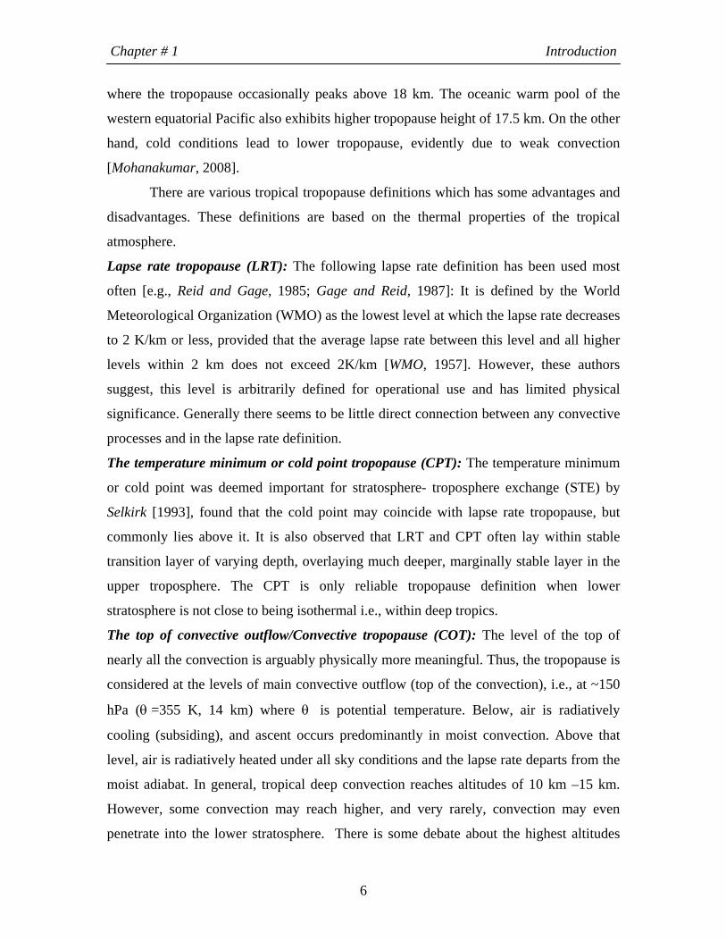
The top of convective outflow/Convective tropopause (COT): The level of the top of

nearly all the convection is arguably physically more meaningful. Thus, the tropopause is

considered at the levels of main convective outflow (top of the convection), i.e., at ~150

hPa (θ =355 K, 14 km) where θ is potential temperature. Below, air is radiatively

cooling (subsiding), and ascent occurs predominantly in moist convection. Above that

level, air is radiatively heated under all sky conditions and the lapse rate departs from the

moist adiabat. In general, tropical deep convection reaches altitudes of 10 km –15 km.

However, some convection may reach higher, and very rarely, convection may even

penetrate into the lower stratosphere. There is some debate about the highest altitudes

6


reached by convection, with evidence that it may go as high as 19 km (θ = 420 K), well

above the CPT (θ = 380 K) [Sherwood, 2000]. However, such events are very infrequent

and the frequency of convection drops rapidly with altitude above the COT [Holton,

1995]. Tropical rainfall measuring mission (TRMM) measurements suggest that only

about 0.1% of the tropics have convection reaching the CPT at any given time.

Clear-sky radiative tropopause (CSRT): The level of zero radiative heating under clear-

sky conditions is called the clear sky radiative tropopause. The CSRT is typically at 14-

16 km. The level of zero radiative heating under clear-sky conditions is slightly higher

than COT. This level is another candidate tropopause, from a radiative-dynamical

perspective.

The 100 hPa level: The 100 hPa level surface has been used as a proxy for the tropical

tropopause, for example by Mote et al, [1996], because of its direct availability from

models. The 100 hPa level is sometimes used as a surrogate for the tropical tropopause

[Frederick and Douglass, 1983].

Tropical tropopause layer (TTL): TTL is the region between the COT and the CPT. The

notion of a 'tropical tropopause layer’ between the CPT and the COT was revived by

Atticks and Robinson [1983] and, more recently by Highwood and Hoskins [1998]. Based

on the overall radiative-convective balance, one might regard the TTL as being more

stratospheric than tropospheric in character.

The factors that determine the altitude and physical properties of the tropical

tropopause is not fully understood, although twin fact is that the troposphere is heated

from below by the surface and that the stratosphere is heated internally by direct

absorption of solar radiation, guarantee that a temperature minimum must exist.

1.4. Annual Variation of the Tropical Tropopause

Several studies of the relative contribution of the radiative effect and dynamical

heat transfer to the formation of the tropopause [Staley, 1957] have been carried out. The

ultimate driving force for the radiative and dynamical effects in the atmosphere is the

intensity of the solar radiation. Gage and Reid [1981] argued that the tropopause

properties are related to small changes in the sea surface temperature (SST) and

consequent change in the intensity of cumulus convection and hence upward branch of

7


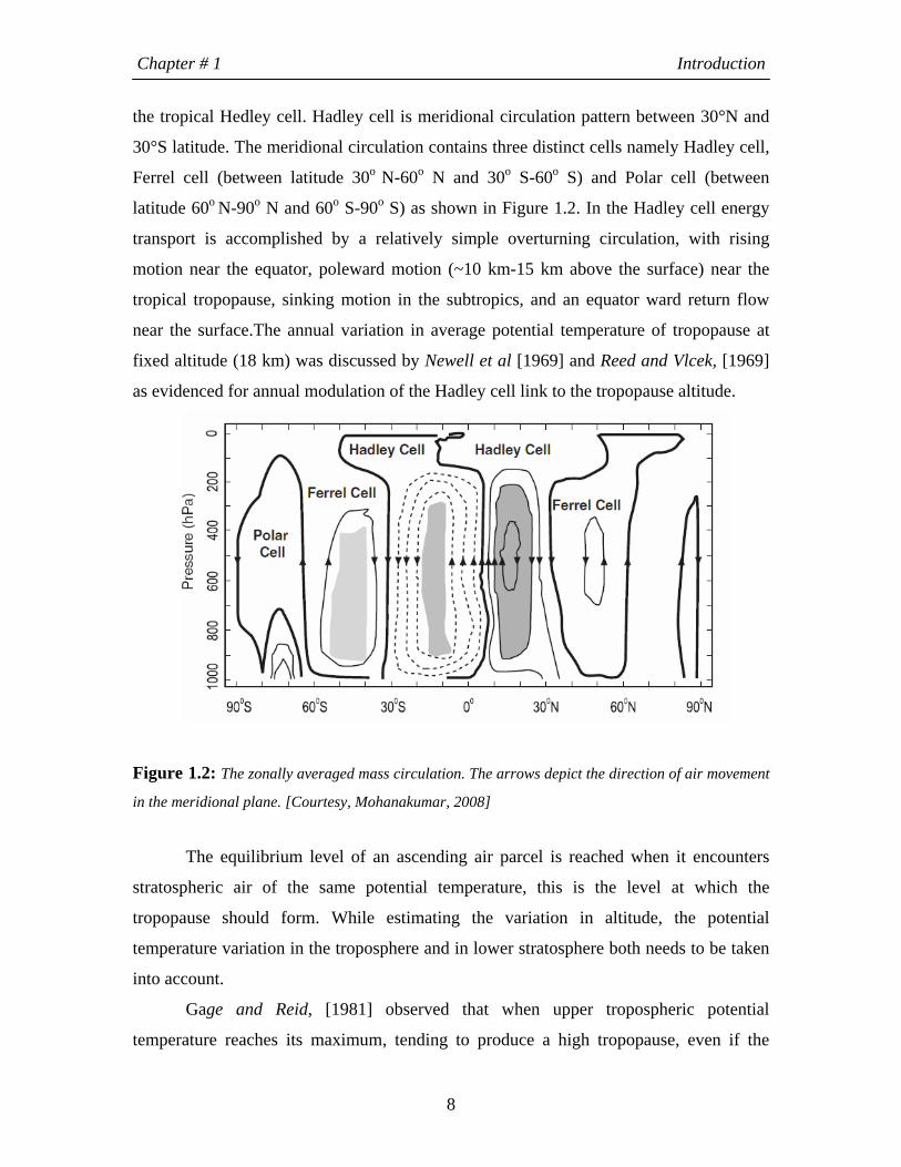
the tropical Hedley cell. Hadley cell is meridional circulation pattern between 30°N and

30°S latitude. The meridional circulation contains three distinct cells namely Hadley cell,

Ferrel cell (between latitude 30o N-60o N and 30o S-60o S) and Polar cell (between

latitude 60o N-90o N and 60o S-90o S) as shown in Figure 1.2. In the Hadley cell energy

transport is accomplished by a relatively simple overturning circulation, with rising

motion near the equator, poleward motion (~10 km-15 km above the surface) near the

tropical tropopause, sinking motion in the subtropics, and an equator ward return flow

near the surface.The annual variation in average potential temperature of tropopause at

fixed altitude (18 km) was discussed by Newell et al [1969] and Reed and Vlcek, [1969]

as evidenced for annual modulation of the Hadley cell link to the tropopause altitude.

Figure 1.2: The zonally averaged mass circulation. The arrows depict the direction of air movement

in the meridional plane. [Courtesy, Mohanakumar, 2008]

The equilibrium level of an ascending air parcel is reached when it encounters

stratospheric air of the same potential temperature, this is the level at which the

tropopause should form. While estimating the variation in altitude, the potential

temperature variation in the troposphere and in lower stratosphere both needs to be taken

into account.

Gage and Reid, [1981] observed that when upper tropospheric potential

temperature reaches its maximum, tending to produce a high tropopause, even if the

8

http://en.wikipedia.org/wiki/Tropopause


stratospheric potential temperature were constant. In fact, associated increase in the

adiabatic cooling (possibly combined with variation in stratospheric ozone concentration)

causes minimum in the lower stratospheric temperature also causing an increase in the

tropopause altitude. These two effects usually reinforce each other, amplifying in the

change in the tropopause altitude. Further Reid and Gage [1981] observed that the annual

variation in the thermal field in the lower stratosphere is found to out of phase with

tropospheric variation. The annual variation in the tropopause altitude is thus attributed to

(1) the annual variation in the tropical surface insolation that causes (2) the annual

variation in the sea surface temperature, which in turn causes (3) a variation in the

absolute humidity of surface air that (4) give rise to annual variation in potential

temperature at tropopause and lower stratosphere. This is summarized in Figure 1.8.

The annual cycle of tropical has been linked to seasonal variations in solar

radiation and its impact on tropical convection [Reid and Gage, 1981; Shimizu and Tsuda,

2000] and to remote forcing during boreal winter associated with the intensification of

the Brewer-Dobson circulation (discussed in section 1.11) [Yulaeva et al., 1994, Reid

and Gage, 1996]. The upwelling Brewer-Dobson circulation in the tropical stratosphere

is driven by a combination of effects including wave drag, transient radiative driving, and

the stratospheric (i.e. non-convective) Hadley circulation. The annual variation of the

CPT is important for understanding water vapour transport in and through the TTL. The

CPT temperature not only affected by large scale process but also by small scale forcing

by convective clouds and waves resulting from clouds, to the ultimate drivers such as sea

surface temperatures. Tropopause temperature changes may occur through direct

radiative effects, radiative-convective effects or indirect dynamical effects (through

changes to the Brewer Dobson circulation).

1.5. The Interannual Variation

Gage and Reid, [1982] observed that Interannual and annual variation in the

thermal field of lower stratosphere and upper troposphere are out of phase. The

interannual and annual variations are explained as response of the variations of incoming

solar radiation. These responses include direct radiative effects (diabatic heating) and

indirect dynamical effects similar interpretations were made by Reid and Gage, [1981]

9


and Gage and Reid, [1981]. Based on their approach, Gage and Reid, [1982] proposed

that the convective activity is modulated by changes in solar radiation and that the

temperature field in the troposphere responds positively to increase in convective activity.

This positive response is due to a combination of the release of latent heat within

convective cells and adiabatic heating due to subsidence in the environment of

thunderstorms. In the lower stratosphere the collective effect of changing thunderstorm

activity is to modulate the intensity of the ascending branch of the Hadley circulation.

When thunderstorm activity is at a maximum, strong ascent in the Hadley cell cools the

lower stratosphere adiabatically as suggested by Newell et al. [1969] and Reed and Vlcek,

[1969]. Conversely, when the thunderstorm activity is at a minimum and the troposphere

is relatively cold, the lower stratosphere is relatively warm.

Following Reid and Gage, [1981] the annual forcing is attributed to annual

variation in solar radiation received at tropical latitudes. The response of the lower

stratosphere is out of phase with the tropospheric variations due to the response of the

varying Hadley circulation. Gage and Reid, [1981] have suggested that inter-annual

variations represent the atmospheric response to a small variation of the insolation that

was positively correlated with solar-activity cycle. Interannual variations in the tropical

tropopause have been linked to the quasi-biennial oscillation of the equatorial

stratosphere, the El Nin˜o-Southern Oscillation and episodic volcanic eruptions.

Tropopause Variation with Solar Cycle: The variation of the tropopause altitude is found

increased with increased sunspot number (Stranz, [1959]; Rasool, [1961]). Based on the

model as discussed earlier the potential temperature at the tropopause is calculated which

was consistent with the observation with some deviation which were attributed due to

solar activity. The observed variation in the altitude of the tropical tropopause can thus be

explained if the solar constant varies by less than 1% during course of the 11-year cycle

of solar activity [Gage and Reid, 1981]. Wilson et al,[1980] repotted that an increase of

0.4% solar luminosity between rocket-born radiometer flight during June 1976 and

November 1978, an interval in which monthly mean sunspot number increased from 12

to 97. Based on the observation, it is further indicated that tropical ocean acts as a vast

water bath that responds to small changes in the sun’s radiative output, and that the

10


resulting small changes in the average sea surface temperature are magnified at the

tropopause through medium of the latent heat release in deep cumulus convection in the

tropics.

The increase in UV radiation will increase the potential temperature in the lower

stratosphere that lead to lowering the tropopause. However, tropopause may lower due to

dynamics which is not clear at present. The connection between the solar output and

tropopause has implications in the global climate [Gage and Reid, 1981].The temperature

in the tropical lower stratosphere is determined by the competition among three deriving

forces, to which fourth has to be added if perturbation in the atmospheric constituents,

especially volcanic aerosols are taken into account. The three forcings fluctuations are (1)

the normal seasonal cycle, (2) the quasi biennial oscillation in zonal winds, and (3) the

ENSO related effects.

1.6. The Quasi-Biennial Oscillation

The quasi-biennial oscillation (QBO) in stratospheric winds and temperatures is

discovered by Reed et al., [1961] and Veryard and Ebdon [1961] and has been

investigated from several decades (e.g. Plumb and Bell, [1982]; Naujoket, [1986]) .The

mean-flow interaction involving upward propagating wave from troposphere has been

generally accepted as a explanation for the QBO [Holton and Lindzen, 1972; Plumb,

1977]. This oscillation has the following observed features: (i) zonally symmetric easterly

and westerly wind regimes alternate regularly with periods varying from about 24 to 30

months, (ii) successive regimes first appear above 30 km, but propagate downward at a

rate of 1 km month−1, (iii) the downward propagation occurs without loss of amplitude

between 30 and 23 km, but there is rapid attenuation below 23 km, and (iv) the oscillation

is symmetric about the equator with maximum amplitude of about 20 m s−1, and an

approximately Gaussian distribution in latitude with a half-width of about 12o [Andrews

et al., 1987].

Departures from the regular seasonal cycle are dominated by the QBO in the

middle stratosphere, and the QBO continues to exert an important influence in the lower

stratosphere, where it interacts with the annual cycle. The net result of this interaction is

to modulate the amplitude of the annual cycle, producing a weak cycle when the QBO

11


effect opposes the normal cycle and a strong cycle when it reinforces it. The interaction

appears to take place mainly in northern winter months, however, when the annual cycle

is in its cool phase, while variations in northern summer months are significantly smaller.

Since the QBO itself is nearly biennial, the modulation that it produces in the annual

cycle has a strong biennial component, i.e., weak and strong cycles tend to alternate. The

quasi biennial forcings at higher altitudes is thus turned into a biennial variation in the

lower stratosphere that is phase locked to the annual cycle.

The detailed relationship between the QBOs in wind and temperature has been

discussed by several authors [e.g., Reed, 1964; Dunkerton and Delisi, 1985]. The

essential points, however, are clear from the thermal wind equation, which can be written

approximately as:

zuy

gRT

yT

∂∂Ω

−=∂∂ 2 (1.1)

in the vicinity of the equator, where , and are the zonal wind speed (m/s),

temperature and distance (meter) from the equator, respectively,

u T y

Ω , and g R are the

Earth’s rotational angular velocity, gravitational acceleration, and radius. Inserting

numerical values this equation becomes

zuTy

yT

∂∂

×−=∂∂ −12103.2 (1.2)

A typical value for the vertical shear in the QBO wind at the equator is about 30

m/s in 6 km or about 0.005 s-1. Taking a typical undisturbed temperature of ~ 210 K, a

variation of the order of 2 to 4 K occurs within 10o of the equator, which was found

comparable with annual cycle [Reid, 1994].

The period is found close to well known QBO in tropical stratospheric zonal

winds [e.g., Wallace, 1974] and a similar QBO in global tropopause pressure has

identified by Angell and Korshover [1964, 1974]. Reid and Gage, [1985] found the

difference between high and low ~ 0.3 km in the tropopause QBO. The interpretation of

the tropopause QBO is not clear, however, they link its maxima and minima occurring

during easterly phase and westerly phase of the QBO. Reed, [1962] shown that the QBO

component of the zonal wind was in geostrophic balance even at that near-equatorial

latitude. Since warm stratosphere implies a low tropopause (assuming that upper

12


troposphere is not equally warmed) the minimum in tropopause altitude should occur

close to westerly wind maxima at the base of the stratosphere. The swing in temperature

just above the tropopause that accompanies the swing in the tropopause altitude can be

estimated by assuming that the tropopause follows as isentropic surface as temperature

changes. Using the standard definition of the potential temperature ,

tropopause altitude (pressure) can be related through (taking log and differentiating);

288.0)/1000( pT=θ

PdPTdT /288.0/ = (1.3)

For the peak to peak QBO swing in the tropopause altitude of about 300 m

corresponds of about 5.4 hPa. Therefore substituting in equation (1.3) together with

average tropopause pressure and temperature of values of 100 hPa and 192 K,

respectively, the temperature swings ~ 3 K were observed in the lower stratosphere just

above the tropopause. The QBO in tropopause altitude can thus be tentatively attributed

to the corresponding QBO in lower stratospheric temperature, which is itself probably

consequence of the weak vertical motion needed to maintain geostrophic balance in the

zonal wind field. However, later Zhou et al., [2001] reported that the QBO signature in

the tropical CPT is probably caused by the downward-propagating QBO meridional

circulation (computed by Plumb and Bell, [1982]) in the equatorial stratosphere. Zhou et

al., [2001] observed that that the westerly shears at 50 hPa, which are accompanied by

warm temperature anomalies [Plumb and Bell 1982], lead the tropical CPT temperatures

by about 6 months and are positively correlated with the tropical CPT temperatures. The

westerly shear at 50 hPa takes about 3–4 months to reach 100 hPa while easterly shear 5-

6 months to propagate from 50 hPa to 100 hPa [Naujoket 1986]. The stratospheric QBO

signatures in the tropical CPT are mainly zonally symmetric.

1.7. El Niño—Southern Oscillation (ENSO)

The east–west pressure gradient associated with the Walker circulation undergoes

an irregular interannual variation. This global scale “see-saw” in pressure, and its

associated changes in patterns of wind, temperature, and precipitation, was named the

southern oscillation by Walker as shown in Figure 1.3. The surface pressure anomalies at

Darwin Australia and Tahiti are negatively correlated and have strong variations in the

period range of 2–5 years. During normal condition the high pressure with cold water at

13


Peru and low pressure and warm water at Darwin exists which drive the trade wind from

west to east, while abnormally the pressure reverse between the Peru and Darwin which

cause El Niño. These patterns of reversal occur in the period range of 2–5 years known as

the E1 Nino/Southern Oscillation.

ENSO events clearly cause an additional variation in the tropical lower

stratospheric temperature, again with main effect occurring in northern winter months.

The simplest explanation is based on the thermodynamics is that the warming takes place

in the tropical troposphere during ENSO warm events, presumably caused by increase in

latent heat release, is compensated by cooling in higher regions, where there is no

internal heat source. Assuming there is some upper level above which ENSO effect

vanish, the average temperature below this level, as reflected by it geopotential height,

must be unchanged. Since the troposphere warms, the overlaying upper troposphere and

stratosphere must cool. That is, the thermal expansion of the troposphere implies a

contraction of the lower stratosphere, since geopotential heights are unchanged above the

“capping” level, and a contraction at constant pressure must be accompanied by a

decrease in temperature.

Figure 1.3: Schematic diagram of the equatorial Walker Circulation [Courtesy : Webster, 1983]

There is general agreement that the principal dynamical deriving force for the

tropical atmosphere is provided by the release of the latent heat accompanying deep

cumulus convection [e.g., Holton, 1979]. A saturated air parcel that is carried up in the

core of deep convective cloud has its potential temperature increased to high values by

14


latent heat release, and buoyancy forces prevent it from sinking again once it reaches the

vicinity of the tropopause. Since net radiative heating rates near the tropical tropopause

are small [Manabe and Hunt, 1968], the air that leaves the core of one of these clouds is

likely to remain for some time at tropopause levels, spreading laterally outward to merge

with the (potentially) warm air from other clouds. This horizontal spreading can be

directly seen in the rapid dispersion of volcanic dust clouds around the tropics [e.g.,

Barth et al., 1983] and is probably the agent responsible for the spatial averaging of

tropopause properties that is seen in the similarity of the annual variation in altitude all

over the tropics [Reid and Gage, 1981]. The tropopause peak may be amplified through a

coincidental combination of a cool stratosphere caused by the QBO and a warm

troposphere caused by the high SST. In previous section it is motioned that the annual

cycle of the zonal mean tropical tropopause is driven by extratropical stratospheric wave

forcing [Yulaeva et al. 1994], but the zonal asymmetrics in the tropical tropopause can be

attributed to the direct response of the atmosphere to a large-scale region of tropospheric

diabatic heating [Highwood and Hoskins 1998]. Using ECMWF data [Zhou et al ,

2001b ] characterized the ENSO signatures in the CPT which shows distinct East–West

dipole and North–South dumbbell features.

1.8. Equatorial Intraseasonal Oscillation

In addition to the interannual variability associated with El Niño, the equatorial

circulation has an important intraseasonal oscillation, which occurs on a timescale of 30–

60 days and is often referred to as the Madden–Julian oscillation (MJO) in honor of the

meteorologists who first described it. The structure of the equatorial intraseasonal

oscillation is shown schematically in Figure 1.4, which shows the time development of

the oscillation in the form of longitude–height sections along the equator, with time

increasing at an interval of about 10 days for each panel from top to bottom. The

circulations in Figure1.4 are intended to represent anomalies from the time-mean

equatorial circulation. The oscillation originates with development of a surface low-

pressure anomaly over the Indian Ocean, accompanied by enhanced boundary layer

moisture convergence, increased convection, warming of the troposphere, and raising of

15


the tropopause height. The anomaly pattern gradually moves eastward at about 5ms−1 and

reaches maximum intensity over the western Pacific.

Figure 1.4: Longitude-height section of the anomaly pattern associated with the tropical intraseasonal oscillation (MJO). Reading downward the panels represent a time sequence with intervals of about 10 days. Streamlines show the west–east circulation, wavy top line represents the tropopause height, and bottom line represents surface pressure (with shading showing below normal surface pressure). [After Madden, 2003; adapted from Madden and Julian, 1972.]

16


As the anomaly moves over the cooler waters of the central Pacific, the

anomalous convection gradually weakens, although a circulation disturbance continues

eastward and can sometimes be traced completely around the globe. The observed

interaseasonal oscillation is known to be associated with equatorial Rossby and Kelvin

waves.

1.9. Vertically Propagating Equatorial Waves

Vertically propagating gravity waves in the presence of rotation for a simple

situation in which the Coriolis parameter was assumed to be constant and the waves were

assumed to be sinusoidal in both zonal and meridional direction. Such inertia–gravity

waves can propagate vertically only when the wave frequency satisfies the inequality

Nf <<ν . Thus, at middle latitudes, waves with periods in the range of several days are

generally vertically trapped (i.e., they are not able to propagate significantly into the

stratosphere). As the equator is approached, however, the decreasing Coriolis frequency

should allow vertical propagation to occur for lower frequency waves. Thus, in the

equatorial region there is the possibility for existence of long-period vertically

propagating internal gravity waves. Both Kelvin and Rossby–gravity modes have been

identified in observational data from the equatorial stratosphere. The observed

stratospheric Kelvin waves are primarily of zonal wave number s = 1 and have periods in

the range of 12–20 days. An example of zonal wind and temperature oscillations caused

by the passage of Kelvin waves at a station Singapore near the equator is shown in the

form of a time–height section in Figure1.5 (a) and (b) during the descending westerly

phase of the QBO. However, from Figure 1.5 it is clear that the downward propagation of

the perturbation with period between speed maxima of about 12 days and a vertical

wavelength (computed from the tilt of the oscillations with height) of about 6–7 km. As

shown in Figure 1.5 (c) of the temperature field for the same period reveal that the

temperature oscillation leads the zonal wind oscillation by 1/4 cycle (i.e., maximum

temperature occurs prior to maximum westerlies), which is just the phase relationship

required for upward propagating Kelvin waves. Additional observations from other

stations indicate that these oscillations do propagate eastward at the theoretically

17


predicted speed. Therefore, there can be little doubt that the observed oscillations are

Kelvin waves.

Figure1.5: (a) Zonal wind perturbation (b) Temperature perturbation and (c) perturbation average

for altitude 16-18 km observed over Singapore during March-May 2002.

The existence of the Rossby–gravity mode has been confirmed in observational

data from the stratosphere in the equatorial Pacific. This mode is identified most easily in

the meridional wind component, as v is a maximum at the equator for the Rossby–gravity

mode. The observed Rossby–gravity waves have s = 4, vertical wavelengths in the range

of 6–12 km, and a period range of 4–5 days. Kelvin and Rossby–gravity waves each have

significant amplitude only within about 20 latitude of the equator. A more complete

comparison of observed and theoretical properties of the Kelvin and Rossby–gravity

modes is presented in Table 1.1. In comparing theory and observation, it must be recalled

that it is the frequency relative to the mean flow, not relative to the ground, that is

18


dynamically relevant. It appears that Kelvin and Rossby–gravity waves are excited by

oscillations in the large-scale convective heating pattern in the equatorial troposphere.

Although these waves do not contain much energy compared to typical tropospheric

weather disturbances, they are the predominant disturbances of the equatorial

stratosphere, and through their vertical energy and momentum transport play a crucial

role in the general circulation of the stratosphere. In addition to the stratospheric modes

considered here, there are higher speed Kelvin and Rossby–gravity modes, which are

important in the upper stratosphere and mesosphere. There is also a broad spectrum of

equatorial gravity waves, which appears to be important for the momentum balance of the

equatorial middle atmosphere.

Table1.1: Characteristics of the Dominant Observed Planetary-Scale Waves in the Equatorial Lower Stratosphere [After Andrews et al., 1987].

Theoretical description Kelvin wave Rossby–gravity wave Discovered by Wallace and Kousky

(1968) Yanai and Maruyama (1966)

Period (ground-based) 2π/ω 15 days 4–5 day Zonal wave number s = ka cos φ

1–2

4

Vertical wavelength 2 π/m 6–10 km 4–8 km Average phase speed relative to ground

+25 m s−1

–23 m s−1

Observed when mean zonal flow is

Easterly (maximum≈−25m s−1)

Westerly (maximum≈ +7 m s−1)

Average phase speed relative to maximum zonal flow

+50 m s−1

–30 m s−1

Approximate observed amplitudes u′ 8 m s−1 2–3 m s−1 v′ 0 2–3 m s−1 T ′ 2–3 K 1 K

1.10. Stratosphere-Troposphere Exchange

In the tropics, it has been suggested that a tropical tropopause layer (TTL) spans

the transition region from the convectively dominated overturning circulation of the

19


Hadley cell to the region of slow upwelling (primarily wave-driven) of the lower

stratospheric Brewer-Dobson circulation. In general, the transport between stratosphere

and troposphere takes place in two ways (i) along the isentropic surfaces which may

occur adiabatically (wavy arrows in Figure 1.6) and (ii) across the isentropic surfaces,

which may require diabatic processes, including three-dimensional turbulent process.

Figure 1.6: Dynamical aspects of the stratosphere-troposphere exchange. The tropopause is shown

by thick line (blue). Thin lines are isentropic or constant potential surface temperature labeled in

kelvins. The wavy double headed arrows denote meridional transport by eddy motions [After

Holton et al, 1995].

Since, the tropopause intersects the isentropes, transport can occur in either way

and likely to occur in both ways. In the UTLS region consisting of the isentropic surfaces

that intersect the tropopause, air and chemical constituent can be irreversibly transported

20


as adiabatic motions lead to large latitudinal displacements of the tropopause followed by

irreversible mixing on small scales. From the knowledge of the eddy effects, the extra-

tropical stratosphere and mesosphere act non-locally on the tropics as global scale fluid

dynamical suction pump. The pumping action is slow but inexorable and causes large-

scale upward transfer of mass from the tropical troposphere into the tropical stratosphere,

at rate that is largely independent of local condition near the tropical tropopause. Indeed,

on contrary, as pointed out by Yulaeva et al. [1994] and Rosenlof [1995], the local

condition must respond to the pumping rate, insofar as stronger extra-tropical pumping

must tend to pull tropical UTLS temperature below radiative equilibrium, encouraging

deep cumulonimbus and producing higher and colder tropopauses.

Also well known are the fact that water vapor shows similar upward extending

plume, but that in contrast with aforementioned tracers, very low values of the water

vapor mixing ratio extends upward from a minimum within a few kilometers of the

tropical tropopause. The minimum mixing ratio is only a few parts per million by volume

(ppmv) and far lower than the tropospheric values. It is generally accepted, with good

reason, that the basic mechanism responsible for the low values is freeze drying [Brewer,

1949] a process in which air passing through the tropical tropopause has its water vapor

mixing ratio reduced to ice saturation value at or near the tropopause. Recently

Sathiyamurthy and Mohanakumar, [2000] and Mohanakumar and Pillai [2008] observed

the relation between tropospheric biennial oscillation (TBO) and QBO which indicates

troposphere-stratosphere interaction over Indian monsoon region.

1.11. Brewer-Dobson circulation

The Brewer-Dobson circulation is a slow circulation pattern, first proposed by

Brewer to explain the lack of water in the stratosphere. The Brewer-Dobson Circulation

is an equator-to-pole circulation pattern that features slow lifting motion in the tropics

and sinking motion in the polar latitudes. This tropical lifting circulation out of the lower

stratosphere is quite slow, of the order of 20-30 m per day. Lifting by the Brewer-Dobson

Circulation carries ozone out of its tropical lower and middle stratosphere, which is the

photochemical source region, into the lower polar stratosphere, where it accumulates due

to sinking motion. He presumed that water vapor is freeze-dried as it moves vertically

21


through the cold equatorial tropopause. Dehydration can occur in this region by

condensation and precipitation as a result of cooling to temperatures below 193 K. The

lowest values of water are found just near the tropical tropopause. Later Dobson

suggested that this type of circulation could also explain the observed high ozone

concentrations in the lower stratosphere polar regions which are situated far from the

photochemical source region in the tropical middle stratosphere. The Brewer-Dobson

circulation additionally explains the observed latitudinal distributions of long-lived

constituents like nitrous oxide and methane. That Brewer-Dobson circulation is

controlled by stratospheric wave drag, quantified by the Eliassen-Palm flux divergence,

sometimes lays claim to the extratropical pump, with the circulation at any level being

controlled by the wave drag above that level. However, the wave drag can be difficult to

compute accurately and it is common to diagnose the mean circulation from the diabatic

heating. It is possible to estimate the net mass flux across a given isentropic surface from

the diabatic heating. Figure 1.7 shows the average annual flow of the Brewer Dobson

Circulation.

Figure: 1.7 Zonal mean middle atmospheric circulation and annual average ozone density (DU/km),

from Nimbus-7 SBUV Observations during the period 1982–89 [Courtesy: NASA]

1.12. The Stratospheric Fountain

Kley et al. [1979] reported measurements over Brazil of stratospheric water vapor

mixing ratios of just 3 ppmv at an altitude of about 21 km. This value corresponds to a

22


frost point of about -89oC at that altitude or about -84oC at 16 km which is approximately

the altitude of tropical tropopause. The local temperature of the tropical tropopause was

only about -80oC and therefore passage of air through this region could not have been

responsible for drying the air. Kley et al. [1979] suggest that the stratospheric air must

have entered from troposphere in another geographical region where tropopause is close

to frost point necessary to remove the moisture (i.e., ~ -84oC) assume that the largest

vertical motion into stratosphere occurs where the temperature are lowest. If lower limit

of the stratospheric water vapor contains is ~ 3.5 ppmv that corresponds to a mass mixing

ratio of 2.2 µg g-1 which is close to the minimum values reported by Mastenbrook. The

corresponding frost points are -84oC at 80 hPa and -82.4oC at 100 hPa. Newell and

Stewart, [1981], selected critical temperature at 100mb and assumes that air which has

reached this low temperature by 100m can pass into the stratosphere without altering the

stratospheric humidity. Therefore the area outlined by the -82.4oC isotherm at 100 hPa

represents the region where air may enter the stratosphere. Areas where air enters the

stratosphere from the troposphere are west pacific in the December-February; northern

South America in January-March and in May-September, Bay of Bengal, India and

Malaysia. In general, the fountains are most active in October-March and moves to the

monsoon region for the Northern Hemisphere summer.

1.13. The Extratropical Pump

To understand the STE, the existence of nonlocal dynamical effects in the

atmosphere is to be taken into account. Reorganization of the nonlocal effects is crucial

for understanding any fluid-dynamical system that supports fast waves whose travel

times are short in comparison with other time scale of interest. For example to understand

why air moves towards the inlet of any suction pump, one needs to recognize that the

travel times of the acoustic waves are short in the sense and that there is corresponding

nonlocal effect. Mass conservation has a key role and for practical purposes, acts

instantaneously, as a nonlocal constraint. The time delay between turning on the pump

and establishment the flow towards suction tube is order of an acoustic propagation time,

usually negligible of all the time scale of interest. This non local picture is to be

contrasted with statements like “air moves toward the suction tube because the pressure-

23


gradient force pushes it,” which miss the point that the pressure gradient adjusts

nonlocally, to fit in with mass mass-conservation constraint.

There is a fundamentally similar nonlocal effects having direct relevance to the

STE problem, namely the effect extratropical stratosphere and mesosphere on the tropical

stratosphere. This depends on the fact that the global-scale travel times of acoustic waves

and large scale gravity waves are short in comparison with other time scale of interest.

The effect has been demonstrated, indeed has been intensively studied, in the dynamical

literature beginning with pioneering work of Eliassen [1951] and Dickson [1968]. These

and many other studies have shown that the extratropical stratosphere and mesosphere as

a kind of global scale fluid dynamical suction pump, driven by certain eddy motions. The

distinction between tropics and extratropics arises from the Earth’s rotation, on which

extratropical pumping action depends. The word “suction” is that statistically speaking,

the most important of the eddy motions, so called “breaking Rossby waves” and related

potential vorticity transporting motions, have ratchet like character related to the sense of

Earth’s rotation.

Figure1.8: Schematic diagram of the factors that determine the altitude of the tropical tropopause

(modified after Reid and Gage, [1981])

Radiation Balance

Solar Radiation

Sea Surface Temperature

Humidity

Hadley Circulation Convection(Vertical Motion)

Tropopause Altitude

Solar Stratospheric TemperatureRadiation

Extra-tropical forcings

Brewer-Dobson Circulation

Eliassen Palm Flux

24


These eddy effects has a strong tendency to add up and give persistently one-way

pumping action, whose strength varies seasonally and interannually and air gradually

withdrawn from tropical stratosphere and pushed poleward and ultimately downward.

Where air parcel are being pulled upward (as in tropical stratosphere), adiabatic cooling

pulls temperature below their radiative values and where air parcels are being downward

(as happens most strongly in high latitudes in winter and spring), adiabatic warming

pushes temperatures above their radiative values. This mechanically pumped global-scale

circulation is often referred as the “wave driven circulation”.

1.14. Thesis Layout

All previous sections dealt with the factors affecting the tropical tropopause right

from the seasonal to solar cycle variations. In general, understandings of the tropopause

behavior on these time scale are well established. However, in short scales, particularly

day-to-day and sub-daily scales, characteristics of the tropopause, which are equally

important is least explored due to limitations in the existing techniques. In addition, large

scale features affecting the tropopause are dealt by assuming zonal mean variation.

However, there are large longitudinal behavior exist which was paid less attention until

now. The tropical tropopause has been studied in past but they are meager because of the

limited data sets. In addition, the existing tropical tropopause studies are mainly focused

on the western pacific region and the studies over monsoon region which is expected to

behave differently is yet to be done. By using the daily radiosonde launching and

simultaneous MST radar observations along with GPS RO data an attempt has been made

to study the tropical tropopause behavior with special emphasis on the Indian monsoon

region. The tropopause over the Indian monsoon region is found to be highest during

winter season when convection is week. What causes the winter high tropopause, whether

the extra-tropical wave forcing is the only answer? There are many such issues remain

unexplained. This thesis is intended to find the reasons for few such questions. Thus,

keeping in mind of these limitations in previous works the present thesis attempts to

overcome some of these limitations by utilizing the measurement from the state of art

techniques like MST Radar and GPS Radiosonde observation together with high vertical

resolution and high accuracy GPS RO measurements.

25


The following are the objectives attempted in the present thesis.

1) How the tropospheric convective outflow level is compared with altitude of

minimum potential temperature gradient and what is its relation to brightness

temperature? What is the nature of the tropical tropopause layer over Indian

monsoon region?

2) How tropical tropopause parameters vary in various scales (ranging from seasonal

to sub daily scale) especially over Indian monsoon region? Does a sub-daily

variation show any diurnal or semidiurnal component? How tropical tropopause

parameters are associated with convection, especially on short term?

3) Whether the tropical tropopause shows longitudinal behavior, if it is so, why? At

which region it has the pronounced longitudinal characteristics? Does tropical

tropopause show different characteristics in convectively active (west pacific and

Indian monsoon) and non –active region?

4) How the multiple tropopauses which commonly appear in the tropical region can

be interpreted? Are the existing (WMO) definitions are adequate to quantify the

multiple structure of the tropical tropopause or new definition is needed?

5) How the tropical tropopause is modulated by equatorial Kelvin wave during

different seasons and different phases of the quasi-biennial oscillation (QBO)?

The complete work is distributed in eight chapters and content of each chapter is

briefly summarized below

A brief introduction about the tropical tropopause properties based on present

understanding is presented in Chapter1.

As mentioned earlier, to attempt these issues, the MST radar, GPS Radiosonde

observation at Gadanki (13.5o N, 79.2o E), and Global positioning system (GPS) Radio

occultation (RO) observations in the tropical belt (±30o) are used. Descriptions of each

system are provided in Chapter 2.

Chapter 3 establishes the concept of the convective tropopause using MST radar

vertical velocity observations at Gadanki, a tropical station. This is compared with the

26


altitude of local minimum of potential temperature lapse rate obtained from simultaneous

radiosonde observations. The convective tropopauses altitudes are also compared with

the cloud top altitudes obtained using satellite brightness temperature.

Chapter 4 presents detail features of the tropical tropopause characteristics and its

variability over the Indian monsoon region with special emphasis on the variation of

tropical tropopause on shorter time (sub-daily) scales. The shorter-term (sub-daily)

variability of the cold point tropopause is also examined in relation to convection and

tidal modulation.

Chapter 5 characterizes the longitudinal variability of the tropical tropopause,

tropical convective tropopause and TTL using radiosonde and GPS RO data. In this study

the behavior of the tropopause in pacific (convective region), non-pacific and Indian

monsoon region is emphasized. There are several studies (eg. Geller et al, 2002) has been

carried for the longitudinal characteristics of the tropical tropopause. However present

study of tropical tropopause over Gadanki reveals some new longitudinal characteristics

when compare to pacific and non pacific region, which are not reported earlier.

Chapter 6 deals with characteristics of the multiple tropopauses (MTs) in the

tropics using Radiosonde and GPS RO data. The multiple tropopauses are mainly focused

on the mid-latitude regions which are found associated with subtropical jet streams.

These reports show that the MTs in the tropical region are less explored since the

occurrences are very few. The present study shows that less number of occurrences of

MTs over tropical region is restricted due to threshold value used in WMO criteria. In

this study an alternative criterion is proposed which is based on the cold point tropopause

and points of inflection rather than lapse rate as in WMO criteria. Based on present

method the annual variation of occurrence statistics of MTs (LT ST and TT) is studied by

using several radiosonde stations data within the tropical region. Using GPS RO

observations, the inter-annual variation in altitude, temperature and pressure in different

longitude sector divided into 60o grid are presented. The physical processes responsible

for the formation of MT above and below the cold point are also discussed.

27


Chapter 7 deals with the tropical tropopause modulation by equatorial waves in

different seasons. The main focus of this chapter is to quantify the seasonal behavior of

the Kelvin wave/ Rossby gravity wave which play dominant role in the modulation of the

tropical tropopause. The modulation of the tropical tropopause in easterly phase, westerly

phase and transition zone of easterly and westerly phase of quasi biennial oscillation

(QBO) is discussed briefly. The spectrum analysis has been performed to extract the

dominant period.

Chapter 8 describes the summary drawn from the present study. Few suggestions

and recommendations for further studies are also briefly outlined.

---END---

28

studies on the characteristics oftropical...

Documents