studies in informatics and control · mircea ivanescu, mihaela cecilia florescu, nirvana popescu,...
TRANSCRIPT

STUDIES IN INFORMATICS AND CONTROL
With Emphasis on Useful Applications of Advanced Technology
Volume 17 • Number 2 • 2008
Informatics and Control Publications

EDlTORlAL ORGANIZATION Editor-in-Chief: Prof. F.G. Filip Member of the Romanian Academy
Journal Manager: Andrei Niculescu Editorial Office: ICI Bucharest Desktop Publishing: Coroleucă Daniela 8-10 Averescu Avenue
011455 Bucharest 1, Romania EDlTORlAL BOARD
Dr. Neculai Andrei National Institute for R&D in Informatics 8-10 Averescu Avenue, 71316 Bucharest Romania
Prof. Dr. Doina Banciu National Institute for R&D in Informatics 8-10 Averescu Avenue, 71316 Bucharest Romania Dr. Jacques Bernussou Laboratoire d'Automatique et d'Architecture des Systemes C.N.R.S./LAAS 7, avenue du Colonel Roche 31077 Toulouse France Prof. Pierre Borne Ecole Centrale de Lille Cité Scientifique-BP 48 F 59651 Villeneuve d'Ascq Cedex France Prof. DSc. Kiril Boyanov Bulgarian Academy of Sciences Laboratory for Parallel and Distributed Processing Acad. G. Bonchev Bl. 25A,Sofia 1113 Bulgaria Prof. Franco Davoli Universita di Genova Facolta di Ingegneria, Dipart. Inf., Sistemistica, Telematica via Opera Pia, 11A, 16145 Genova Italy Prof. Guy Doumeingts GRAI Université Bordeaux 351, cours de la Libération 33405 Talence Cedex France
Prof. dr. Ion Dumitrache Department of Computer Sc ience "Politehnica" University of Bucharest 313 Splaiul Independentei, 77206 Bucharest Romania Dr. Constantin Gaindric Institute of Mathematics of Moldavian Academy of Sciences 5, Academiei str., Kishinev, 277028 The Republic of Moldova Prof. José Cláudio Geromel Universidade Estadual de Campinas P.O. B. 6-l0l, 13081 Campinas Brazil Prof. Cristian Giumale Department of Computer Science "Politehnica" University of Bucharest 313 Splaiul Independentei,77206 Bucharest Romania Prof. Peter P. Groumpos Laboratory of Automation and Robotics Electrical Engineering Department University of Patras, Rion 26500 Greece
Prof. Guido Guardabassi Dipartimento di Elettronica Politecnico di Milano Piazza Leonardo da Vinci, 3220133 Milano Italy
Prof. Marius Guran Department of Computer Science "Politehnica" University of Bucharest 313 Splaiul Independentei, 77206 Bucharest Romania Prof. dr. Gunnar Johannsen University of Kassel Systems Engineering and Human Machine Systems, D-34109 Kassel Germany Prof. Claude Kaiser Conservatoire National des Arts et Métiers 292, Rue Saint Martin, 75141 Paris - Cedex 03 France Dr. Eugene J. H. Kerckhoffs Subfaculty of Technical Mathematics and Informatics Delft University of Technology Zuidplantsoen 4, 2628 BZ Delft The Netherlands Prof. Norihisa Komoda Department of Information Systems Engineering Faculty of Engineering Osaka University 2-1 Yamadaoka, Suita,565-0871 Japan Dr. George L. Kovacs CIM Research Laboratory Computer and Automation Research Institute Kende u. 13-17 1111 Budapest Hungary Prof. Andrew Kusiak Industrial Engineering College of Engineering The University of Iowa 4132 Engineering Bldg. Iowa City, IOWA 52242-1527 U.S.A. Prof. Luis M. Camarinha-Matos Departamento de Engenharia Electrotecnica Faculdade de Ciências e Tecnólogia Universidade Nova de Lisboa Quinta da Torre-2825 Monte Caparica Portugal
Prof. dr. Constantin V. Negoita Department of Computer Science Hunter College City University of New York 695 Park Avenue New York, N.Y. 10021 U.S.A Prof. Shimon Y. Nof School of Industrial Engineering Purdue University Grissom Hall, West Lafayette, IN 47907 U.S.A. Dr. Theodor Dan Popescu Process Control System Laboratory National Institute for R&D in Informatics 8-10 Averescu Avenue, 71316 Bucharest Romania Prof. Dr. H. Puta Fakultät für Informatik und Automatisierung Technische Hochschule Ilmenau PSF-327, D-6300 Ilmenau (Thür.) Germany
Prof. Daniel J. Power College of Business Administration University of Northern Iowa Cedar Falls, IA 50614-0125, U.S.A
Prof. Peter D. Roberts Control Engineering Centre School of Engineering City University Northampton Square, London EC1V oHB United Kingdom Dr. Vasile Sima Process Control Systems Laboratory National Institute for R&D in Informatics 8-10 Averescu Avenue, 71316 Bucharest Romania Dr. Florin Stãnciulescu Syst. Analysis, Modelling &Simulation Dept. National Institute for R&D in Informatics 8-10 Averescu Avenue, 71316 Bucharest Romania Achim Sydow GMD-FIRST Forschungsinstitut für Rechnerarchitektur und Softwaretechnik Kekulestraße 7, D 12489 Berlin Germany Prof. Hiroyuki Tamura Department of Systems Engineering Faculty of Engineering Science, Osaka University 1-1 Machikaneyama-cho, Toyonaka, Osaka 565 Japan Dr. Gheorghe Tecuci Center for Artificial Intelligence George Mason University 4440 University Drive,Science and Tech. II Rm 413 Fairfax, VA 22030-4444 U.S.A. Dr. Dan Tufis Centre for Advanced Research in Machine Learning, Natural Language Processing and Conceptual Modelling , Casa Academiei Calea 13 Septembrie 13, Room 1-238, 74311 Bucharest Romania Prof. Subhash Wadhwa Indian Institute of Technology, New Delhi India Prof. Andrew B. Whinston Department of Management Science and Information Systems The University of Texas at Austin CBA 5202 Austin, TXS 78712-1175 U.S.A. Prof. Theodore J. Williams Purdue University Purdue Laboratory for Applied Industrial Control A.A. Potter Engineering Center West Lafayette IN 47907 U.S.A. Prof. dr. Radu Popescu-Zeletin GMDInstitut für Offene Kommunikationssysteme Kaiserin-Augusta Allee 31, D-10589 Berlin Germany Prof. Ying-Ping Zheng Chinese Association of Automation P.O. B. 2728, Beijing 100080 The People's Republic of China
CONTENTS
EDITORIAL
1. BAI-WU WAN, XIAO-E RUAN, DING LIU
New Results in Control of Steady-State Large-Scale Systems 123
2. KAZIMIERZ DUZINKIEWICZ, ADAM BOROWA , KRZYSZTOF MAZUR, MICHAŁ GROCHOWSKI, MIETEK A. BRDYS, KRZYSZTOF JEZIOR
Leakage Detection and Localisation in Drinking Water Distribution Networks by MultiRegional PCA 135
3. ERIC DUVIELLA, PASCALE CHIRON, PHILIPPE CHARBONNAUD
Networked Hydrographical Systems: A Reactive Control Strategy Integrating Time Transfer Delays 153
4. FATMA TANGOUR, PIERRE BORNE
Presentation of Some Metaheuristics for the Optimization of Complex Systems 169
5. A. CHAMROO, I. SIMEONOV, C. VASSEUR, N. CHRISTOV
On the Piecewise Continuous Control of Methane Fermentation Processes 181
6. MIRCEA IVANESCU, MIHAELA CECILIA FLORESCU, NIRVANA POPESCU, DECEBAL POPESCU
A Compliance Control of a Hyperredundant Robot 189
7. MOUNIR AYADI, JOSPEH HAGGÈGE, SOUFIÈNE BOUALLÈGUE, MOHAMED BENREJEB
A Digital Flatness-based Control System of a DC Motor 201
8. FLORIN LEON, MIHAI HORIA ZAHARIA, DAN GÂLEA
Emergent Dynamic Routing Using Intelligent Agents in Mobile Computing 215
9. PASCALE ZARATÉ
Decision Making Process: A Collaborative Perspective 225
10. SVETLANA COJOCARU
Computational Environment Generation for Computer Algebra Systems 231
AUTHOR INDEX


Studies in Informatics and Control, Vol. 17, No. 2, June 2008 123
New Results in Control of Steady-State Large-Scale Systems
Bai-Wu Wan1, Xiao-E Ruan2, Ding Liu3
1The State Key Laboratory for Manufacturing Systems, Xi’an Jiaotong University, P. R. China.
Email: wanbw @mail.xjtu.edu.cn
2Department of Mathematics, Faculty of Science, Xi’an Jiaotong University, P. R. China
Email: wruanxe@ mail.xjtu.edu.cn
3School of Automation, Xi’an University of Technology, P. R. China,
Email: [email protected]
Abstract: This paper reviews what the first Author and his Group have been investigating for the past fifteen years in the on-line steady-state hierarchical intelligent control and optimization of large-scale industrial processes (LSIP), or large-scale systems (LSS), viz., the use of neural networks for identification and optimization, the use of expert system to solve some kind of hierarchical multi-objective optimization problems, the use of the fuzzy logic control, and the use of the iterative learning control. Several implementation examples and the product quality control for LSS are introduced too. Finally the paper suggests the new stage of development.
Keywords: Large-scale systems, industrial control, intelligent control, optimization, quality control
Professor Bai-Wu Wan received his B.S. degree in Electrical Engineering in 1949 and graduated from The Institute of Communication, in 1951 after two year postgraduate study both from the Jiaotong University, Shanghai (no degree system at that time). He was in charge of the Automatic Control Group (now called Department) from 1958-1978, and then he was in charge of The Large Scale Systems Group of Systems Engineering Institute, Xi'an Jiaotong University from 1978-1995. Now, as a professor of Control and Systems Engineering he works with the State Key Laboratory for Manufacturing Systems and Institute of Systems Engineering, Xi'an Jiaotong University. He is a Honorary Member of The Council of Chinese Association of Automation. He was the Member of editorial board for three top Chinese journals of automatic control, and for The Proceedings of Institution of Mechanical Engineers, Part I, Journal of Systems and Control Engineering, United Kingdom; and is the Member of Technical Committee of Large Scale Systems of International Federation of Automatic Control (IFAC). His main research interests are: large scale systems theory and application, quality control, intelligent control. More than 400 papers have been published or accepted in domestic and international journals or proceedings of conferences. He published six books including two monographs "On-line Hierarchical Steady-state Optimizing Control of Large-scale Industrial Processes" and “Optimization and Product Quality Control of Large-scale Industrial Systems”.
Associate Professor Xiao-E Ruan received B.S. and M.S. degrees in Mathematics from Shaanxi Normal University, Xi’an, P.R.China, in 1988 and 1995, respectively and PhD degree in Control science and Engineering from Institute of Systems Engineering, Xi’an Jiaotong University in 2002. Since 1995, she has been with the Department of Mathematics, Faculty of Science, Xi’an Jiaotong University, Xi’an, P.R.China. From March 2003 to August.2004, Dr. Ruan worked as a post-doctoral researcher with the Department of Electrical Engineering and Computer Science, Korea Advanced Institute of Science and Technology. Her current research field includes steady state hierarchical optimization of large-scale industrial processes, iterative learning control and fuzzy logic techniques, etc.
Professor Ding Liu was born in Shandong, China in 1957. He received the B.S and M.S degrees in Department of Automation and Information Engineering, Xi’an University of Technology, Xi’an, China in 1982 and 1987 respectively, and the Ph.D. degree in 1997 from Xi’an Jiaotong University, Xi’an, China. He was a visiting scholar from 1991 to 1993 in University of Fukui, Japan. He is currently a professor, doctoral advisor, and President of Xi’an University of Technology. He has published a book and more than 100 papers, many of them were indexed by SCI, EI, and ISTP. His research interests include complex system’s modeling and control, visual servo, intelligent robot control, digital signal processing and intelligent control theory.
1. Introduction
In the 7-th IFAC/IFORS/IMACS Symposium on Large Scale Systems Theory and Application, Beijing, China, Roberts, the first Author of this paper and Lin (1992) gave a plenary report entitled “Steady-state Hierarchical Control of Large-scale Industrial Processes: A Survey”. It considered the development of hierarchical control of LSIP in three stages: static multilevel optimization stage, steady-state hierarchical optimization stage and integrated system optimization and parameter estimation (ISOPE) stage . Fifteen years and more have passed by since then. What has been emerging in this field? And what is the fourth stage if existed?

Studies in Informatics and Control, Vol. 17, No. 2, June 2008 124
For the past decade, the intelligent control has been a very important research direction and pushing the control science and technology forward. So do the large-scale systems theory and applications. The steady-state intelligent control of industrial processes means the application of ideas and methodologies of artificial intelligence to steady-state hierarchical control of LSIP and LSS based on human experience and knowledge in control and decision. In other words the neural networks, the expert systems (the intelligent decision unit), the fuzzy logic control, the iterative learning control, the genetic algorithms etc. and their combinations are integrated with traditional analytical approach for solving the identification, control, optimization, coordination and fault diagnosis of LSIP and LSS (Wan, 1994). Since the beginning of 1990’s the first Author and his Large-scale Systems Research Group have devoted themselves to the study of steady-state hierarchical intelligent optimizing control of LSIP and LSS for fifteen years. A brief summary of the main research results including the implementation examples in process industry and the conclusions is as follows.
2. Use of Neural Networks
2.1 Neural network modelling
The first Author’s Group has successfully applied a multi-layer BP neural network for identifying a steady-state model of a hot-cold water mixer pilot plant that includes two subprocesses, heating and levelling, and conducted hierarchical optimizing control based on the neural network steady-state model by three microcomputers in hierarchy, and hierarchical steady-state stochastic optimizing control with variance analysis even if the data are corrupted by noise (Wang, Wan and Song, 1994).
For steady-state modelling of process possessing stochastic or chaotic steady-state behaviours, Luo, Liu and Wan (1998) have proposed an adaptive fuzzy neural inferring network (AFNI network) based on Takagi-Sugeno fuzzy model. And the Group have used the neural networks for product quality model and yield model for control of LSS.
2.2 Neural network optimization
Leung, Li and Wan (1993) have used the Hopfield neural network to fit the static optimization with the interaction prediction and the interaction balance coordination methods. The Lagrange multiplier, Kuhn-Tucker multiplier and relax variable are applied to treat constraints, and an energy function E is defined. Then by differentiating E with respect to output y, set-points c and the Lagrange multiplier, Kuhn-tucker multiplier and the relax variable, a set of differential equations are obtained. This set of differential equations is solved by Runge-Kutta method without iteration. It is because the differential equation represented by upper coordinative network and those represented by lower decision networks are solved step by step and simultaneously, and they interchange the integration information step by step within integration.
The first Author’s Group have proved the stability and optimality of Hopfield network (Leung, Li and Wan, 1993; Li, Wan and Leung 1994; 1995; Wan and Huang, 1998). In addition, the Hopfield network has been extended to solve the steady-state optimizing control of LSIP with global feedback or local feedback. It requires 6 on-line iterations to obtain an improved suboptimal solution or 9 on-line iterations to obtain an optimal solution for a LSIP with three subprocesses, respectively. The former result is obtained by using the output shift method, while the latter by output shift and its partial derivative compensation.
3. Use of Expert System
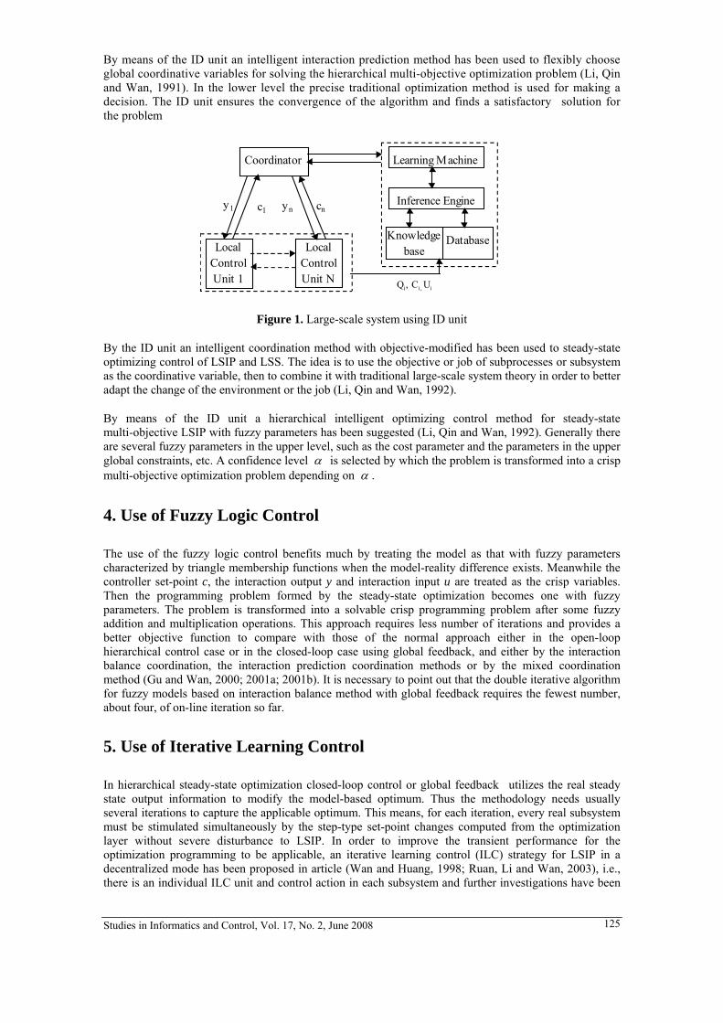
Based on the expert system (rule-based system) an intelligent decision (ID) unit has been suggested to solve some kinds of optimization problems of LSIP and LSS. The ID unit is composed of a knowledge base, a database, an inference engine and a learning machine (Fig.1).
Studies in Informatics and Control, Vol. 17, No. 2, June 2008 125
By means of the ID unit an intelligent interaction prediction method has been used to flexibly choose global coordinative variables for solving the hierarchical multi-objective optimization problem (Li, Qin and Wan, 1991). In the lower level the precise traditional optimization method is used for making a decision. The ID unit ensures the convergence of the algorithm and finds a satisfactory solution for the problem
Coordinator Learning Machine
Inference Engine
Knowledgebase
cn
LocalControlUnit 1
LocalControlUnit N Qi, Ci, Ui
Database
ync1y1
Figure 1. Large-scale system using ID unit
By the ID unit an intelligent coordination method with objective-modified has been used to steady-state optimizing control of LSIP and LSS. The idea is to use the objective or job of subprocesses or subsystem as the coordinative variable, then to combine it with traditional large-scale system theory in order to better adapt the change of the environment or the job (Li, Qin and Wan, 1992).
By means of the ID unit a hierarchical intelligent optimizing control method for steady-state multi-objective LSIP with fuzzy parameters has been suggested (Li, Qin and Wan, 1992). Generally there are several fuzzy parameters in the upper level, such as the cost parameter and the parameters in the upper global constraints, etc. A confidence level α is selected by which the problem is transformed into a crisp multi-objective optimization problem depending on α .
4. Use of Fuzzy Logic Control
The use of the fuzzy logic control benefits much by treating the model as that with fuzzy parameters characterized by triangle membership functions when the model-reality difference exists. Meanwhile the controller set-point c, the interaction output y and interaction input u are treated as the crisp variables. Then the programming problem formed by the steady-state optimization becomes one with fuzzy parameters. The problem is transformed into a solvable crisp programming problem after some fuzzy addition and multiplication operations. This approach requires less number of iterations and provides a better objective function to compare with those of the normal approach either in the open-loop hierarchical control case or in the closed-loop case using global feedback, and either by the interaction balance coordination, the interaction prediction coordination methods or by the mixed coordination method (Gu and Wan, 2000; 2001a; 2001b). It is necessary to point out that the double iterative algorithm for fuzzy models based on interaction balance method with global feedback requires the fewest number, about four, of on-line iteration so far.
5. Use of Iterative Learning Control
In hierarchical steady-state optimization closed-loop control or global feedback utilizes the real steady state output information to modify the model-based optimum. Thus the methodology needs usually several iterations to capture the applicable optimum. This means, for each iteration, every real subsystem must be stimulated simultaneously by the step-type set-point changes computed from the optimization layer without severe disturbance to LSIP. In order to improve the transient performance for the optimization programming to be applicable, an iterative learning control (ILC) strategy for LSIP in a decentralized mode has been proposed in article (Wan and Huang, 1998; Ruan, Li and Wan, 2003), i.e., there is an individual ILC unit and control action in each subsystem and further investigations have been
Studies in Informatics and Control, Vol. 17, No. 2, June 2008 126
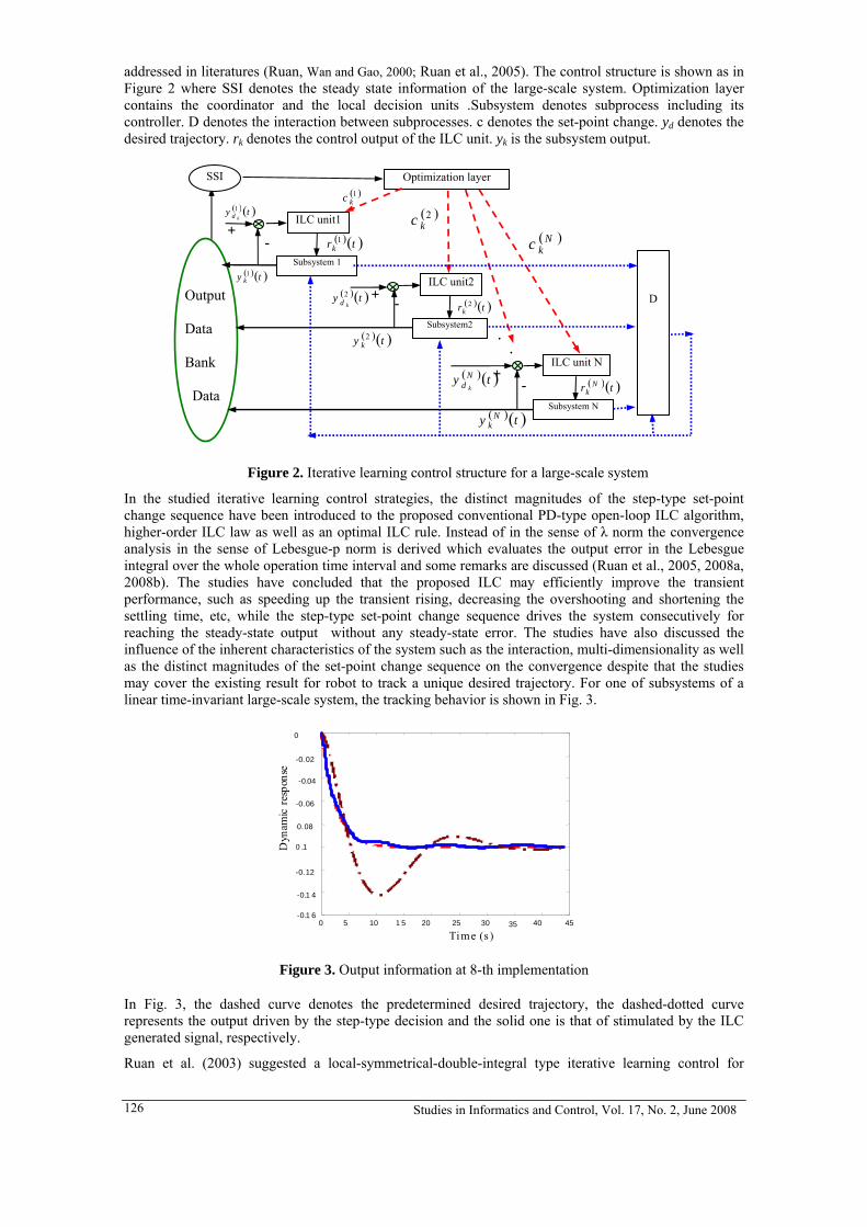
addressed in literatures (Ruan, Wan and Gao, 2000; Ruan et al., 2005). The control structure is shown as in Figure 2 where SSI denotes the steady state information of the large-scale system. Optimization layer contains the coordinator and the local decision units .Subsystem denotes subprocess including its controller. D denotes the interaction between subprocesses. c denotes the set-point change. yd denotes the desired trajectory. rk denotes the control output of the ILC unit. yk is the subsystem output.
Fig.2 Iterative learning control structure for a large-scale system
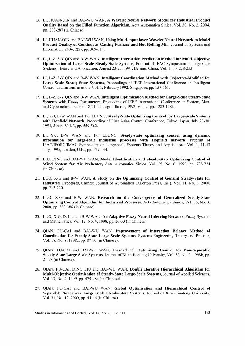
In the studied iterative learning control strategies, the distinct magnitudes of the step-type set-point change sequence have been introduced to the proposed conventional PD-type open-loop ILC algorithm, higher-order ILC law as well as an optimal ILC rule. Instead of in the sense of λ norm the convergence analysis in the sense of Lebesgue-p norm is derived which evaluates the output error in the Lebesgue integral over the whole operation time interval and some remarks are discussed (Ruan et al., 2005, 2008a, 2008b). The studies have concluded that the proposed ILC may efficiently improve the transient performance, such as speeding up the transient rising, decreasing the overshooting and shortening the settling time, etc, while the step-type set-point change sequence drives the system consecutively for reaching the steady-state output without any steady-state error. The studies have also discussed the influence of the inherent characteristics of the system such as the interaction, multi-dimensionality as well as the distinct magnitudes of the set-point change sequence on the convergence despite that the studies may cover the existing result for robot to track a unique desired trajectory. For one of subsystems of a linear time-invariant large-scale system, the tracking behavior is shown in Fig. 3.
0 5-0.1 6
-0.1 4
-0.12
-0 .1
-0.08
-0.06
-0.04 -0.02
0
10 1 5 20 25 30 35 40 45
Time (s )
Dyn
amic
res
pons
e
Figure 3. Output information at 8-th implementation
In Fig. 3, the dashed curve denotes the predetermined desired trajectory, the dashed-dotted curve represents the output driven by the step-type decision and the solid one is that of stimulated by the ILC generated signal, respectively.
Ruan et al. (2003) suggested a local-symmetrical-double-integral type iterative learning control for
. .
.
( )( )ty k1
+ -
+
Subsystem2
( )( )tr Nk
+-
Figure 2. Iterative learning control structure for a large-scale system
Output Data Bank
Data
Optimization layer SSI
( )Nkc
( )2kc
( )1kc
( )( )trk1
ILC unit1 ( ) ( )ty
kd1
Subsystem 1
( )( )trk2
( )( )ty k2
ILC unit2 ( )( )ty
kd2
-
( )( )ty Nk
ILC unit N ( )( )ty Nd k
Subsystem N
D

Studies in Informatics and Control, Vol. 17, No. 2, June 2008 127
dynamics of industrial processes with time delay in the course of steady-state optimization when measurement noise is present.
This approach is a combination of study on the steady-state hierarchical optimization with that on the transient. It is evident that after seven ILC iterations the dynamic characteristics are greatly improved with two periods of set-points being provided by the coordinator in the Optimization layer of Fig.2. Furthermore, the first ILC iteration in the second optimization period is equivalent to the k+1-th iteration in the first optimization period if its number of iterations is k. Therefore the dynamic characteristics are further improved in the second period. Thus the whole set-point changes can once be fully imposed on the LSIP or LSS with little disturbance.
6. Applications in Industry
The first example is the steady-state optimizing control of a nickel flash furnace based on neural network models in a smelting plant (Wan, Wan and Yuan, 1999) which is located in Jinchang City, Gansu Province, China (Fig. 4). The quality model of the matte is based on three 5×5×1 BP neural networks.
The inputs of the quality model are the 4 manipulating variables and 1 disturbing variable, while 3-quality indexes (properties of matte) are the outputs. The matte yield model is based on a 5×5×1 BP neural network with yield as the output. Then the objective function is minimization of the total energy consumption of the furnace subject to the inequality constraints formed by quality submodels and quality index tolerances, and product yield model with yield not less than normal. The study and the industrial site experiment for the optimization of the furnace have obtained a satisfactory result.
Liu and the first Author (Liu and Wan, 1999) have given the second example in which a multi-layer BP neural network is used to identify the steady-state model of air preheater of a big power-station boiler under different load condition (Fig. 5).
Stack
Secondary fan
Primary fan
Gas side
Air side
Gas-in venturi
Air-in venturi
Boiler
Coal powder made
Secondary air Primary air
Preheater
Figure 5. Boiler preheater system
The primary wind pressure and temperature, and the secondary wind pressure and temperature of the preheater are used as four inputs and the boiler-load is used as output of neural network. Both data can be measured for training neural network.
The sum of primary wind pressure and secondary wind pressure approximately represents the sum of the
Slag
Acid production
Concentrates
Reaction shaft
Slag clean areaSettler
Off-take gas
Flux Oxygen
Oil
Matte
Dust
Matte
Figure 4. Nickel flash furnace system

Studies in Informatics and Control, Vol. 17, No. 2, June 2008 128
two wind motor currents is selected to be the objective function. The optimization is to minimize the sum of currents under a definite load condition and is carried out by an enumerative method within feasible region latticed by small intervals. Based on this model an on-line steady-state optimizing control is successfully applied. The intelligent optimization gives considerable profit by saving electricity, is really implemented in big power-station boilers in China as well as those exported to abroad.
7. Steady-State Identification
Chen and Wan (1995; 1999) have suggested an approach to identifying a steady-state model by the dynamic data acquired from the normal set-point changes during tuning or optimization. The input is of the step-function form. They have proved, however, that under mild conditions the steady-state model obtained from the approximate dynamic model is with the strongly consistent estimates.
To a class of nonlinear slow time-varying large-scale processes, which have many subprocesses interconnected with one another, a parallel two-stage identification algorithm has been studied. The consistency of the estimates and convergence of the parallel iteration are also proved.
In addition, the Research Group has given a new steady-state identification method that provides a steady-state model of a nonlinear process only using steady-state data from several set-point changes and the estimates are strongly consistent (Huang and Wan, 1997; see Chapter 2, Wan and Huang, 1998). Besides, Huang, Wan and Han (1994) have given a method different from the above by Chen and Wan to calculate the process derivative with respect to set-point only using steady-state data acquired from several times set-point changes and its strong consistency has also been proved.
8. Robustness of Optimization Algorithm
It needs to study robustness of an optimization algorithm with respect to model parameter and noise to avoid divergence. Xu and Wan (1994) have investigated the robust stability of the algorithms for steady-state optimizing control of industrial processes, discussed the dependence of the optimal solution obtained from the algorithms on the parameters λ that represent the characteristic numbers of noises or process structure parameters. The Pompeiu-Hausdorff hemidistance H of two optimal solution sets is used as a measure for the robustness of the algorithm with respect to λ. One is the optimal solution set, while the another is the optimal solution set perturbed by the parameter λ. Actually to calculate the hemidistance is rather difficult, if not impossible. Hence ∂H/ ∂λ is used as a sensitivity index to compare different optimization algorithms. The concept can be used to some simple cases (Xu, Wan and Han, 1997).
9. Generalized Steady-State of Industrial Process
Actually from the point of view of steady-state optimisation the influence of stochastic noise in process variables is often ignored due to its low level and little influence to the objective function. The problem is called stochastic optimising control of steady-state systems, or the systems are under stochastic steady-state (Lin, Han, Roberts and Wan, 1989) if the noise can not be ignored.
Luo and Wan (1999a) have extended the concept of steady-state to a generalized form, i.e., from the point of view of steady-state optimisation, a system may be under several kinds of steady-state that are constant, periodic, quasi-periodic, stochastic, chaotic steady- states in an industrial process or system. Actually some random process happens in a LSIP is often a mixture of the chaotic steady-state with a stochastic steady-state of low level. They have proposed a stringent definition about the generalized steady-state and proved that it exists when the nonlinear process satisfies some conditions. It is proved that the nominal central value of the generalized steady-state uniquely exists when the nonlinear process satisfies some conditions. The time averages of process variables uniformly converge to their respective nominal central values.
According to the definitions of generalized steady-state and the nominal central value of steady-state sets, Luo and Wan (1999a) stringently have described the problem of generalized steady-state optimizing

Studies in Informatics and Control, Vol. 17, No. 2, June 2008 129
control of industrial processes in a finite measure space. Under certain conditions above problem is transformed into a model based equivalent deterministic problem, and an algorithm for solving the problem has been suggested. A chemical process composed of a liquid level control system (LLCS) and a continuously stirred reactor (CSTR) (Fig. 6) has been used for simulation study of generalized steady-state optimizing control.
Luo, Han and Wan (1999) have stringently given a definition for the chaotic steady-state, and proved the existence theorem under some conditions. The chaotic steady-state of a chemical process is simulated. The steady-state modelling is based on an AFNI network (Luo, Liu and Wan, 1998). The global convergence of the steady-state generalized optimizing control algorithm has been proved based on Zangwill’s Theorem of global convergence. Optimality of the optimizing control solution has been studied also (Luo and Wan, 1999b).
10. Global Convexification, Multi-Objective and Non-Separable Optimization Problems
Qian and Wan (2000) have proposed an approach through the p-th power transformation to obtain a global optimal solution by multi-objective optimization technique. The original optimization problem is embedded in a multi-objective optimization problem, then its non-inferior frontier is convexified. The original global optimal solution is picked up from the set of non-inferior solutions. Of course, this approach can be used to solve a multi-objective optimization problem for LSIP. Qian, Liu and Wan, (1999) has proposed a double iterative algorithm for non-separable multi-objective optimization problem which can satisfy the decision maker’s preference.
For non-separable steady-state systems the Group has given an approaches for solving them. It is based on transversal transmission of information among local decision units to decouple the objective function,. Meanwhile the traditional longitudinal transmission of information is used to decouple the interconnection between subsystems (Qian and Wan, 1998a).
Another approach is for non-additive objective functions of general non-separable systems, Qian and Wan (1998b) have suggested a double-loop iterative algorithm. All these algorithms can be used for on-line optimizing control of LSIP.
11. Product Quality Control for Large–Scale Industrial Systems
A continuous casting and hot rolling production line in a Steel Complex in Shanghai is considered as a typical example (Fig.7). Knowledge Discovery in Database (KDD) is used to acquire data from computers of 3rd-generations for controlling the line, and from the computers in chemical analysis lab and material testing lab. To improve the product quality of the continuous casting and hot rolling, it is very necessary and important for a steel complex to find the relationship between the input variables and the product quality, i.e., to establish the steel plate static quality model. The steel plate quality model of a continuous casting furnace and hot rolling mill is a complex nonlinear function which after analysing and discussing with plant engineers Xing decides to include at least 32-input variables: 23 chemical elements variables for casting, 2 heating furnace variables, 7 rolling mill variables and 4-output variables (material testing indexes): rupture elongation rate, tensile strength, yield ratio and impact energy etc (Xing, 2000; Wan, 2002).
A
P ControllerSensor
Qi
Qm
QoCm V
h
LLCS
CSTR
d
Figure 6. LLCS and CSTR

Studies in Informatics and Control, Vol. 17, No. 2, June 2008 130
All data used for modelling are preprocessed. 15, 000 useful sample data are obtained from 30, 000 and more observations in the data warehouse. Among them 9, 026 sample data are complete and can be used for modeling, however, they are corrupted by noise. And a high dimension input BP neural network is firstly chosen for the architecture of the steel plate quality model. To easily train and improve the accuracy the 32-input and 4-output BP neural network is decomposed as four 32-input and 1-output sub-neural network models. It is called the decomposition of the product quality modelling problem based on large-scale neural network.
The precision of modeling is expressed in the percentage of hits, i.e., the total number of hits in all 9, 026 data divided by 9, 026. A hit is defined as that pair of data which makes the model output within an error± 5% of the real output.
Jia, Wan and Feng (2000) give a learning algorithm that each weight of BP neural network is trained separately with large inertia. The percentage of hits for suggested algorithm based on high- dimension -input BP neural network is 81.5%.
11.1 Modelling Based on Wavelet Neural Network
It is important to notice that the sequence of real output is in a saw tooth-like form . For this reason the wavelet neural network (WNN) is a better choice for the modelling problem.
Li and Wan (2002) choose the similar structure of the WNN as that of multi-layer perceptron (MLP), except that here the activation function of hidden nodes is replaced by a B-spline wavelet function of one dimension. Employing the MLP-like architecture, the proposed three layer WNN (1-input, 1-hidden layer and 1-output) is a powerful tool to handle high dimensional problem. The percentage of hits for this quality model is 81.5%, while that for an ordinary BP three layer neural network with the same number of nodes provides a precision 62.7%.
11.2 High-Dimension-Input Wavelet Neural Network Based on Work Procedure of the Technology and Key Inputs
The production line is a serially connected system and 32 input variables start act at different stages according to the work procedure. Therefore Li and Wan (2004a) suggest a WNN with several input layer depending on the work procedure (Fig.8). For instance, in first input layer there are 22 input variables (chemical-element variables ) simulating the casting, in second input layer there are 2 variables simulating the heat furnace, and in the third layer there are 7 variables simulating the rolling. And for this special kind of steel plate there are three most important chemical elements, viz., carbon, manganese and titanium. Their corresponding input variables are connected to the input as well as the output nodes directly. A suitable learning algorithm is given also. The percentage of hits for quality model of this architecture is 93.4%.
Finishing rolling
Initial rolling
temper rolling
Continuous casting machine
Molten steel
Figure 7. Continuous casting and hot rolling
Heating furnace

Studies in Informatics and Control, Vol. 17, No. 2, June 2008 131
Figure 8. The architecture of three-input-layer wavelet neural
network based on work procedure and key inputs - Input node; - Neuron
The further improvement of the precision can be made by clustering all the data and dividing them into 12 groups, and using the modular WNN approach (Li 2003). Then each submodel gives a precision about from 93.4~95% depending on the group of data used in modeling. And using a filled function algorithm to get a global optimum makes the above WNN result further improve 1% of precision (Li and Wan, 2004b; 2004c).
11.3 Application of Product Quality Model to New Product and New Technology Design
More occasionally it is not allowed to change all the manipulating variables in a quality model. Therefore, a new kind model, product quality control model, is suggested in which the input variables are quality index and those variables that are not allowed to change or that are assigned preliminary, and the output variables are some manipulating variables that are allowed to change. By the latter one can find the manipulating variables required from the quality index value (Xing, 2000). For instance, for a certain kind of titanium-manganese alloy steel plate the manipulating variables required or engineers hope to get from the quality control model are the amount of titanium, manganese and carbon. Sometimes the quality control model is more convenient in practice.
manipulating variables from these four submodels is a serious problem for the continuous casting and hot rolling. It is called the coordination or synthesis of the product quality modelling problem based on large-scale neural network. For simple cases the solution is the intersection set of the output manipulating variable sets from the quality control submodels. But in more complicated cases, perhaps, some kind of data fusion is necessary. How to overcome this drawback needs further study. And evidently it needs different kinds of such quality models for different design purposes.
12. Conclusions
The paper concludes that the second stage steady-state hierarchical optimization has extended to generalized steady-state hierarchical optimization and that the third stage ISOPE has extended to ISOPE and DISOPE (dynamic integrated system optimization and parameter estimation) stage, and that the fourth stage is the hierarchical intelligent control and optimization stage. Obviously, the latter is a very important one.
In the Group’s experience the neural network modelling using the data from normal set-point changes, updated by newly coming data, the optimization algorithm selected from different intelligent methods depending upon the nature of the problem, application of iterative learning control technique, and integrated with fault diagnosis
ykx
1x
2x
321 nnnx ++
1nx 11+nx
21 nnx +
121 ++nnx

Studies in Informatics and Control, Vol. 17, No. 2, June 2008 132
is a good choice, it gives great potential for increasing profit. And all these functions can be integrated in intelligent agents for on-line steady-state intelligent hierarchical control of LSIP.
Acknowledgement
The work is supported by the National Natural Science Foundation of China under granted No. F030101-60274055, F030101-60574021, 9674003 and supported by the High Technology Plan (863 plan) No. 863-51-95-011 of P.R. of China. The old version of the work was presented on the 10th IFAC /IFORS /IMACS/IFIP Symposium on Large Scale Systems: Theory and Applications, July 26-28, 2004, Osaka, Japan.
REFERENCES
1. CHEN, Q-X and B-W WAN, Asymptotic Normality Analysis of the Estimation Error of Steady-State Models for Industrial Processes: SISO Case, Int.J. Systems Sci., Vol. 23, No.11, 1992, pp. 2003-2023.
2. CHEN, Q-X and B-W WAN, Steady-State Identification for Large-Scale Industrial Process by Means of Dynamic Models, Int. J. Systems Sci., Vol. 25, No. 5, 1995, pp. 1079-1101.
3. CHEN, Q-X and B-W WAN, A New Approach to Establish a Steady-State Model of an Industrial Process, Int. J. Systems Sci., Vol. 30, No. 10, 1999, pp. 1073-1091.
4. GU, JIA-CHEN and BAI-WU WAN, Interaction Balance Method for Large-Scale Industrial Processes with Fuzzy Parameters, Acta Automatica Sinic, Vol. 28, No. 4, 2002, pp. 569-574, (in Chinese).
5. GU, JIA-CHEN and BAI-WU WAN, Interaction Prediction Method for Large-Scale Industrial Processes with Fuzzy Parameters, Control and Decision, Vol. 16, No. 1, 2001, pp. 58-61 (in Chinese).
6. GU, JIA-CHEN and BAI-WU WAN, Mixed Coordination Method for Large-Scale Industrial Processes with Fuzzy Parameters, Control Theory and Applications, Vol. 19, No. 5, 2002, pp. 763-770 (in Chinese).
7. HUANG, Z-L and B-W WAN, Identification of Steady-State Model for Nonlinear System Described by Volterra Series and Its Strong Consistency, Journal of Xi’an Jiaotong University, Vol. 31, No. 6, 1997, 20-26 (in Chinese).
8. HUANG, Z-L, B-W WAN and C-Z HAN, A New Approach to Estimate the Process Derivative and Its Strong Consistency Analysis, Control Theory and Applications, Vol. 11, No. 1, 1994, pp. 12-19 (in Chinese).
9. JIAO, B-C, C.W. LI and B-W WAN, A Convexifying Approach to Separable Non-Convex Large-Scale Steady-State Systems, Preprint of IFAC/IFORC/IMAC Symposium on Large-scale Systems Theory and Applications, Vol. 1, 11-13, July, 1995, London, U.K., pp. 117-122.
10. LEUNG, T-P, Y-J LI and B-W WAN, Static Hierarchical Optimization of Large-Scale Systems Based on Hopfield Network, Proceedings of the 1-st Chinese World Congress on Intelligent Control and Intelligent Automation, Vol. 1, Beijing, China, Aug. 26-30, 1993, pp. 556-559 (in Chinese).
11. LI, HUAN-QIN and BAI-WU WAN, Product Quality Model Based on High Dimension Input Wavelet Neural Network for Hot Rolling Mill, Proceedings of the 2002 International Conference on Control and Automation, 16-19 June, 2002, Xiamen, China, pp. 60-63.
12. LI, HUAN-QIN and BAI-WU WAN, Multi-input layer Wavelet Neural Network and Its Application, Acta Automatica Sinica, Vol. 30, No. 4, 2004, pp. 939-943 (in Chinese).
Studies in Informatics and Control, Vol. 17, No. 2, June 2008 133
13. LI, HUAN-QIN and BAI-WU WAN, A Wavelet Neural Network Model for Industrial Product Quality Based on the Filled Function Algorithm, Acta Automatica Sinica, Vol. 30, No. 2, 2004, pp. 283-287 (in Chinese).
14. LI, HUAN-QIN and BAI-WU WAN, Using Multi-input layer Wavelet Neural Network to Model Product Quality of Continuous Casting Furnace and Hot Rolling Mill, Journal of Systems and Information, 2004, 2(2), pp. 309-317.
15. LI, L-Z, S-Y QIN and B-W-WAN, Intelligent Interaction Prediction Method for Multi-Objective Optimization of Large-Scale Steady-State Systems, Preprint of IFAC Symposium of large-scale Systems Theory and Application, August 23-25, 1991, Beijing, China, Vol. 1, pp. 228-233.
16. LI, L-Z, S-Y QIN and B-W WAN, Intelligent Coordination Method with Objective-Modified for Large-Scale Steady-State Systems, Proceedings of IEEE International Conference on Intelligent Control and Instrumentation, Vol. 1, February 1992, Singapore, pp. 157-161.
17. LI, L-Z, S-Y QIN and B-W WAN, Intelligent Optimization Method for Large-Scale Steady-State Systems with Fuzzy Parameters, Proceeding of IEEE International Conference on System, Man, and Cybernetics, October 18-21, Chicago, Illinois, 1992, Vol. 2, pp. 1283-1288.
18. LI, Y-J, B-W WAN and T-P LEUNG, Steady-State Optimizing Control for Large-Scale Systems with Hopfield Network, Proceeding of First Asian Control Conference, Tokyo, Japan, July 27-30, 1994, Japan, Vol. 3, pp. 559-562.
19. LI, Y-J, B-W WAN and T-P LEUNG, Steady-state optimizing control using dynamic information for large-scale industrial processes with Hopfield network, Preprint of IFAC/IFORC/IMAC Symposium on Large-scale Systems Theory and Applications, Vol. 1, 11-13 July, 1995, London, U.K., pp. 129-134.
20. LIU, DING and BAI-WU WAN, Model Identification and Steady-State Optimizing Control of Wind System for Air Preheater, Acta Automatica Sinica, Vol. 25, No. 6, 1999, pp. 728-734 (in Chinese).
21. LUO, X-G and B-W WAN, A Study on the Optimizing Control of General Steady-State for Industrial Processes, Chinese Journal of Automation (Allerton Press, Inc.), Vol. 11, No. 3, 2000, pp. 213-220.
22. LUO, X-G and B-W WAN, Research on the Convergence of Generalized Steady-State Optimizing Control Algorithm for Industrial Processes, Acta Automatica Sinica, Vol. 26, No. 3, 2000, pp. 382-386 (in Chinese).
23. LUO, X-G, D. Liu and B-W WAN, An Adaptive Fuzzy Neural Inferring Network, Fuzzy Systems and Mathematics, Vol. 12, No. 4, 1998, pp. 26-33 (in Chinese).
24. QIAN, FU-CAI and BAI-WU WAN, Improvement of Interaction Balance Method of Coordination for Steady-State Large-Scale Systems, Systems Engineering Theory and Practice, Vol. 18, No. 8, 1998a, pp. 87-90 (in Chinese).
25. QIAN, FU-CAI and BAI-WU WAN, Hierarchical Optimizing Control for Non-Separable Steady-State Large-Scale Systems, Journal of Xi’an Jiaotong University, Vol. 32, No. 7, 1998b, pp. 21-28 (in Chinese).
26. QIAN, FU-CAI, DING LIU and BAI-WU WAN, Double Iterative Hierarchical Algorithm for Multi-Objective Optimization of Steady-State Large-Scale Systems, Journal of Applied Sciences, Vol. 17, No. 4, 1999, pp. 479-484 (in Chinese).
27. QIAN, FU-CAI and BAI-WU WAN, Global Optimization and Hierarchical Control of Separable Nonconvex Large Scale Steady-State Systems, Journal of Xi’an Jiaotong University, Vol. 34, No. 12, 2000, pp. 44-46 (in Chinese).

Studies in Informatics and Control, Vol. 17, No. 2, June 2008 134
28. ROBERTS, P. D., B-W WAN and J. LIN, Steady-State Hierarchical Control of Large-Scale Industrial Processes: A Survey, Preprint of IFAC Symposium on large-scale Systems Theory and Application, 23-25 August, 1991, Beijing, Vol. 1, pp. 1-10.
29. RUAN, XIAO-E, BAI-WU WAN and HONG-XIA GAO, The Iterative Learning Control for Saturated Nonlinear Control Systems with Dead Zone, Proc. of the 3-rd Asian Control Conference, 4-7 July, Shanghai, China, 2000, pp. 1554-1557.
30. RUAN, XIAO-E, BAIWU WAN, FENGMIN CHEN, Decentralized Iterative Learning Controllers for Nonlinear Large-Scale Systems to Track Trajectories with Different Magnitudes, Acta Automatica Sinica (Accepted in Nov. 29, 2007).
31. RUAN, X-E, Z. BIEN and K.-H. PARK, Iterative Learning Controllers for Discrete-Time Large-Scale Systems to Track Trajectories with Distinct Magnitudes, International Journal of Systems Science, Vol. 36, No. 4, 2005, pp. 221-233.
32. RUAN, XIAO-E, Z. ZENN BIEN, KWANG-HYUN PARK, Decentralized Iterative Learning Control to Large-Scale Industrial Processes for Nonrepetitive Trajectory Tracking, IEEE Transactions on Systems, Man, and Cybernetics, Vol. 38, No. 1, Jan. 2008, pp. 238-252.
33. RUAN, XIAO-E, HUAN-QIN LI, BAIWU WAN, The Local-symmetrical-double-integral Type Iterative Learning Control for Dynamics of Industrial Processes with Time Delay in Steady-State Optimization, Acta Automatica Sinica, Jan. 2003, Vol. 29, No. 1, pp. 125-129 (in Chinese).
34. WAN, BAI-WU, Product Quality Model and Quality Control Model for Industrial Production and their Applications, Acta Automatica Sinic, Vol. 28, No. 6, 2002, pp. 1019-1024 (in Chinese).
35. WAN, BAI-WU and ZHENG-LIANG HUANG, On-line Steady-state Hierarchical Optimizing Control of Large-scale Industrial Processes, Science Press, Beijing, China, 1998 (in Chinese).
36. WAN, W-H, B-W WAN and J-Y YUAN, Neural Network Modelling and Steady-State Optimizing Control for Nickel Flash Furnace in Smelting Plant, Preprint of 14-th World Congress of IFAC, Beijing, China, Vol. N, 1999.7, pp. 415-420.
37. WANG, W-Y and BAI-WU WAN, Neural Network Identification of Steady-State Process Model Using Dynamic Data, Proceedings of Symposium on Control, Automation Applications (CAI'93), Hong Kong, March 3, 1993, pp. 16-24.
38. WANG, W-Y, B-W WAN and B, SONG, Steady-State Hierarchical Stochastic Optimizing Control of A Mixer Pilot Plant Based on Neural Network Modelling, Proceedings of the 7-th CAA/CACE Science Conference on Process Control, Vol. 1, Qingdao, China, 1994, pp. 5-25 (in Chinese).
39. XING, JIN-SHENG, An Investigation on Steel Plate Quality Model of Large-Scale Hot Rolling Mill Using KDD Technology. [Ph.D. Thesis]. Xi’an Jiaotong University, Xi’an, China (in Chinese).
40. XU, L-J and B-W WAN, Robustness of Optimizing Control Algorithms for Steady-State Industrial Process, Proceeding of First Asian Control Conference, Tokyo, Japan, July 27-30, 1994, Vol. II, pp. 537-540.
41. XU, L-J, B-W WAN and C-Z HAN, Robust Stability and Improved Scheme of Optimizing Control Algorithm for Steady State Industrial Processes, Proceedings of the 2nd Chinese World Congress on Intelligent Control and Intelligent Automation, Vol. II, July 23-27, 1997, Xi’an, China pp. 1190-1194.

Leakage Detection and Localisation in Drinking Water Distribution Networks by MultiRegional PCA
Kazimierz Duzinkiewicz1, Adam Borowa1, Krzysztof Mazur1, Michał Grochowski1, Mietek A. Brdys2, Krzysztof Jezior1
1Faculty of Electrical and Control Engineering, Gdansk University of Technology, ul. Narutowicza 11/12, 80-952 Gdansk, Poland
email: {k.duzinkiewicz; aborowa; k.mazur; m.grochowski; m.brdysl; k.jezior}@ely.pg.gda.pl;
2Department of Electronic, Electrical and Computer Engineering, University of Birmingham, Birmingham B15 2TT, U.K.
email: [email protected]
Abstract: Monitoring is one of the most important steps in advanced control of complex dynamic systems. Precise information about systems behaviour, including faults indicating, enables for efficient control. The paper describes an approach to detection and localisation of pipe leakage in Drinking Water Distribution Systems (DWDS) representing complex and distributed dynamic system of large scale. Proposed MultiRegional Principal Component Analysis (MR-PCA) skilfully takes full advantage of well known PCA method and enables not only for detecting the leakages but also supports their localisation. The main idea of MR-PCA is presented on example of small water network. Next the method is applied to DWDS in Chojnice, northern Poland. DWDS Chojnice is decomposed into suitable subnetworks what makes that the monitoring process is easier and require less sensors. The subnetworks and corresponding PCA monitoring models are selected based on the network operational knowledge and information regarding its topology.
Keywords: Monitoring, large-scale systems, network systems, fault detection algorithms, water leakage detection, statistical methods.
Kazimierz Duzinkiewicz received M.Sc. degree in Electrical Engineering and Ph.D. in Control Engineering from Faculty of Electrical and Control Engineering at Gdansk University of Technology, in 1973 and 1982, respectively. He has been employed as a university teacher starting his work in 1973 from the post of Assistant to the current position of Senior Lecturer in Department of Control Engineering. During his research work he has published over 80 scientific papers and over 50 scientific and technical reports, mainly dealing with following problems: a) production scheduling and operational control of technological systems with switchable processes (refinery type systems), b) computer control of electric power station in emergency conditions, c) safety and reliability analysis of hazardous systems, d) mathematical modelling of complex systems, e) multihorizon and multilevel optimisation, control and decision support structures and algorithms with applications to petroleum industry and environmental systems (drinking water and wastewater systems). He was NOC Chair of the 11th IFAC Symposium on Large Scale Complex Systems, Gdansk, July 23-25, 2007.
Adam Borowa received his M.Sc. degree in Control Engineering in 2002 from Electrical and Control Engineering Department at Gdansk University of Technology. Soon after he became a Ph.D. student in this Department, between 2001 and 2002 he served one’s apprenticeship on Wastewater Treatment Plant at Swarzewo. From 2002 he has been a member of Intelligent Decision Support and Control System Group at Gdansk University of Technology. He was a member of organizing committee of the 11th IFAC Symposium on Large Scale Complex Systems, Gdansk, July 23-25, 2007. He is co-author of 8 publications and 4 chapters in the books. Mainly he focuses on modelling and monitoring of large scale systems, especially processes with many time scales. In 2008 he received the Ph.D. degree in Automatic Control and Robotics.
Krzysztof Mazur received his M.Sc. degree in Control Engineering from Electrical and Control Engineering Department at Gdansk University of Technology in 2005. Currently a Ph.D. student in this Department. A Member of Intelligent Decision Support and Control System Group at Gdansk University of Technology. He was a member of organizing committee of the 11th IFAC Symposium on Large Scale Complex Systems, Gdansk, July 23-25, 2007. His research interests are in the areas of modelling, control and diagnostics of large scale systems. Co-author of 5 papers and 4 chapters in the books.
Michał Grochowski received his M.Sc. degree in Control Engineering in 2000 from Electrical and Control Engineering Department at Gdansk University of Technology. In 2001 he finished M.Sc. study at Faculty of Management and Economics of Gdansk University of Technology. From 1999 to 2003 he was a Ph.D. student in Electrical and Control Engineering Department at Gdansk University of Technology. In 2004 he received the Ph.D. degree in Automatic Control and Robotics. From 1999 is a member of Intelligent Decision Support and Control System Group at Gdansk University of Technology. From 2004 he held the posts of Assistant and Assistant Professor at Control Engineering Department at Gdansk University of Technology. He was a member of organizing committee of the 11th IFAC Symposium on Large Scale Complex Systems, Gdansk, July 23-25, 2007. He is author and co-author of about 15 refereed papers and four chapters in the books. His researches are focused on intelligent control of complex systems, supervisory control, faults detection, softly switched robustly feasible model predictive control.
Mietek A. Brdys received the M.Sc. degree in Electronic Engineering and the Ph.D. and the D.Sc. degrees in Control Systems from the Institute of Automatic Control at the Warsaw University of Technology in 1970, 1974 and 1980, respectively. In 1992 he became Full Professor of Control Systems in Poland. Between 1978 and 1995, he held various visiting faculty positions at the University of Minnesota, City University, De Montfort University and University Polytechnic of Catalunya. Since January 1989, he has held the post of Senior Lecturer in the School of Electronic, Electrical and Computer Engineering at The University of Birmingham. Since February 2001 he has held the post of Full Professor of Control Systems at Gdansk University of Technology. He has served as Consultant for Honeywell Systems and Research Center in Minneapolis, GEC Marconi and Water Authorities in UK, France, Spain, Germany and Poland. His research is supported by the UK and Polish Research Councils, and industry and European Commission. He is author and co-author of about 220 refereed papers and six books. His current research includes
Studies in Informatics and Control, Vol. 17, No. 2, June 2008 135

intelligent decision support and control of complex uncertain systems, robust monitoring and control, softly switched robustly feasible model predictive control. The applications include environmental systems, technological processes, autonomous intelligent vehicles and defence systems. He is a Chartered Engineer, a Member of the IET, a Senior Member of IEEE, a Fellow of IMA and a Chair of IFAC Technical Committee on Large Scale Complex Systems. He was IPC Chair of the 11th IFAC Symposium on Large Scale Complex Systems, Gdansk, July 23-25, 2007.
Krzysztof Jezior received his M.Sc. degree in Control Engineering from Electrical and Control Engineering Department at Gdansk University of Technology in 2007. Since then a Ph.D. student in this Department and a Member of Intelligent Decision Support and Control System Group at Gdansk University of Technology. Focused in his research on modelling and diagnostics of large scale systems. Co-author of 1 publication and 2 chapters in the books.
1. Introduction
Nowadays, monitoring systems besides data gathering are able to pre-process the data, to recover and estimate not directly measured variables. However, in large scale systems there is very large quantity of information that are hard to handle and sometimes almost impossible to properly process and hence to efficiently utilised it in the control process. An example of such systems is Drinking Water Distribution Systems (DWDS) the representatives of the class of network systems. The DWDS are usually, very complex (lots of pipes, connecting nodes, pumps, tanks etc.) and distributed (in space). It entails measuring of very large number of variables necessity, in order to possess information about the system state that is necessary for efficient system control. In such situations special methods enabling for analysis of large amount of data (e.g. faults detection and isolation) are required. Advanced monitoring systems should not only visualize desired data but also be able to detect devices faults and/or the unusual system behaviour. The paper proposes an approach to detecting and localisation of water leakage in pipes by using the Principal Components Analysis (PCA) method [1]. The PCA is a method that looks for multidimensional correlation between the variables and uses it to reduce the dimensionality of problems simultaneously remaining most of original information. Mostly, large amount of real data process do not provide large amount of important information. Hence, PCA explores data to find out very meaningful ones and include them into statistical models. Moreover, these models clearly indicate the abnormal state of the system thanks to specially calculated measures (T2 and SPE). In case of DWDS such a situation might be caused by device faults (e.g. sensor or pump break down), water leakage in pipe, significant increasing of the water uptake (e.g. caused by fire brigades) etc. Detecting of fault is important however, in case of DWDS the system operator still does not know its type and localisation. Leakages detection and localisation issue is a very important and complex problem that has been widely investigated [2] – [6]. However, available active leakage control methods are basically unpractical due to costs or long leak detection and location time [4]. In the paper the novel approach the MultiRegional Principal Component Analysis (MR-PCA) method is used to detect and to locate the water leakage based on measurements from limited number of measuring devices [5]. MR-PCA tries to join operational experience of staff working in water companies and advanced mathematical analysis. Moreover, this method compromises between detection efficiency and a number of measuring devices.
The method is explained based on simple water network and followed with its application to real town case study DWDS Chojnice (northern Poland).
2. Monitoring and Diagnostics in Advanced Control Systems
Monitoring and diagnostics, which purpose is the fault detection and identification issue, are essential elements of advanced control of complex systems (Figure 1) [7] – [9].
Monitoring and diagnostics utilize a variety of methods for solving the fault detection and identification issue. Basically these methods can be divided into tree classes (Figure 2), which are quantitative model-based, qualitative model-based and process history based, also known as data driven methods [7], [10], [11].
Studies in Informatics and Control, Vol. 17, No. 2, June 2008 136

S o f t w e r e
Complex System / Process
Data Acquisition
Supervisor
Control Realisation
Control Evaluation
H a r d w e r e
Fault Detection and Identification
Figure 1. Monitoring and diagnostics (Fault Detection and Identification Unit) in advanced control system structure
Hybrids of monitoring and diagnostic methods can satisfy requirements imposed on a Detection and Identification Unit in a more natural way, since they utilize a set of elements, each fitted to a particular need [7]. Especially if the resulting mixture, consists of different class members, which is the case of MulitiRegional Principal Component Analysis (MR-PCA) [5], [6]. MR-PCA, dedicated to Distributed Systems (DSs) following the network structure, combines Structural Decomposition (SD) and Principal Component Analysis (PCA), where the latter belongs to the Multivariable Statistics methods (Figure 2).
Monitoring and Diagnostic Methods
Quantitative Model-Based
Diagnostic Observers
Parity Space
Extended Kalman Filters
Qualitative Model-Based
Process History Based
Qualitative (Expert Systems, Qualitative Trend Analysis)
Quantitative (Statistical: Multivariable Statistics, Statistical Classifiers, Artificial Neural Networks)
Causal Models (Digraphs, Fault Trees, Qualitative Physics)
Abstraction Hierarchy (Structural Decomposition, Functional Decomposition)
MultiRegional Principal Component Analysis
Figure 2. Monitoring and diagnostic methods classification (based on [10])
The main idea behind SD is to conclude about the conditions of system / process in question by means of its subsystems analysis [11]. PCA is described in the next subsection.
2.1 Principal Component Analysis
Principal Component Analysis is a method, which identifies linear dependencies among variables , resulting in
1>n
nix ,,1K= ns ≤ decorrelated and linearly related variables and a residuals sit ,,1K= snit −= ,,1~
K minimised in the sense of Mean Squared Error (MSE) [1]. Variables are assumed to be normally distributed, with independently, identically distributed (IID) Gaussian noise contamination. Due to statistical consistency condition, PCA can model only quasi-static processes, i.e., with unnoticeable transients, because only cross-correlations between variables are took into account during the identification.
nix ,,1K=
nix ,,1K=
In more details, given a matrix consisting of data collected from the identified process (variables standardized to zero mean and unit variance) and , PCA leads to the following decomposition of :
nN×ℜ∈ΧnN >>
Χ
Studies in Informatics and Control, Vol. 17, No. 2, June 2008 137
TT PTTPΧ ~~+= (1)
where is the scores matrix containing new data vectors corresponding to
original data samples and residuals
sN×ℜ∈T sNj ℜ∈= ,,1Kt
nNj ℜ∈= ,,1Kx sn
Njt −= ℜ∈,,1
~K collected in residual matrix
snN −×ℜ∈T~ . Orthonormal block matrix [ ] nn×ℜ∈PP ~ plays in the decomposition (1) a key role leading
to decorrelation of original cross-correlated data. Its first element , so-called loadings matrix, which column vectors contain linear relations indentified in the data , spans
sn×ℜ∈Pn
si ℜ∈= ,,1Kp Χ s -
dimensional Principal Component Space (PCS), while column vectors nsni ℜ∈−= ,,1
~Kp of the second
snn −×ℜ∈P~ span Residual Space (RS) and both spaces are orthogonal (Fig. 3). Thus Nj ,,1~
K=t and
are projections of on the RS and PCS respectively, where the latter (or P as its basis) is considered as the PCA model.
Nj ,,1K=t Nj ,,1K=x
In order to obtain [ ]PP ~ one can perform diagonalisation (e.g. using Eigen Decomposition (ED)) of
approximated data correlation matrix : nn×ℜ∈XR
XΧRXT
N 11ˆ−
= (2)
resulting in:
[ ] [ TTT PPΛ00Λ
PPRX~
~~ˆ ⎥
⎦
⎤⎢⎣
⎡= ] (3)
where and ss×ℜ∈Λ snsn −×−ℜ∈Λ~ are both diagonal matrices containing eigenvalues of (2): si ,,1K=λ and
sni −= ,,1~
Kλ corresponding to appropriate block matrix of [ ]PP ~ respectively and all eigenvalues are
proportional to the variance of original data in corresponding directions Χ [ ]PP ~ (Fig. 3). In the notation (3)
it is assumed that si ,,1K=λ and sni −= ,,1~
Kλ are sorted in descending order and in particular 1~λλ ≥s . From (2),
(3) it is clear why only cross-correlation process structure can be modelled using PCA approach.
Assumption of IID Gaussian noise contamination leads to equal values of 2,1
~~σλ =−= sni K , where 2~σ is
the variance of noise in question in all sn − residual dimensions. This enables for clear and doubtless separation of and Λ Λ~ , and in consequence and PP ~ . However in practice this is the rare case and one has to choose approximation rather than s s on the basis of some of available methods [12]. The least sophisticated, though quite effective, is the Captured Percent Variance (CPV):
( ) %100~
11
1
∑∑
∑−
==
=
+= sn
ii
s
ii
s
ii
sCPVλλ
λ (4)
where the choice of depend on the assumed minimal captured by the PCA model percent of data variance :
slimCPV
( )( limminargˆ CPVsCPVss
≥= ) (5)
Because of PCA ability of modelling only the linear part of the processes, all nonlinear dependencies contained in data would be linearly approximated minimising MSE of residuals. In such case linearization errors are included in the RS, which becomes a PCS non-fitting data container.
Χ
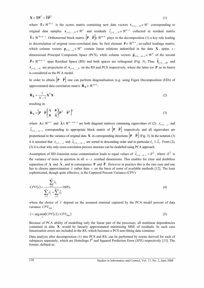
Data analysis after decomposition (1) into PCS and RS, can be performed by norms derived for each of subspaces separately, which are Hottelings T2 and Squared Prediction Error (SPE) respectively [13]. The former, defined as:
Studies in Informatics and Control, Vol. 17, No. 2, June 2008 138
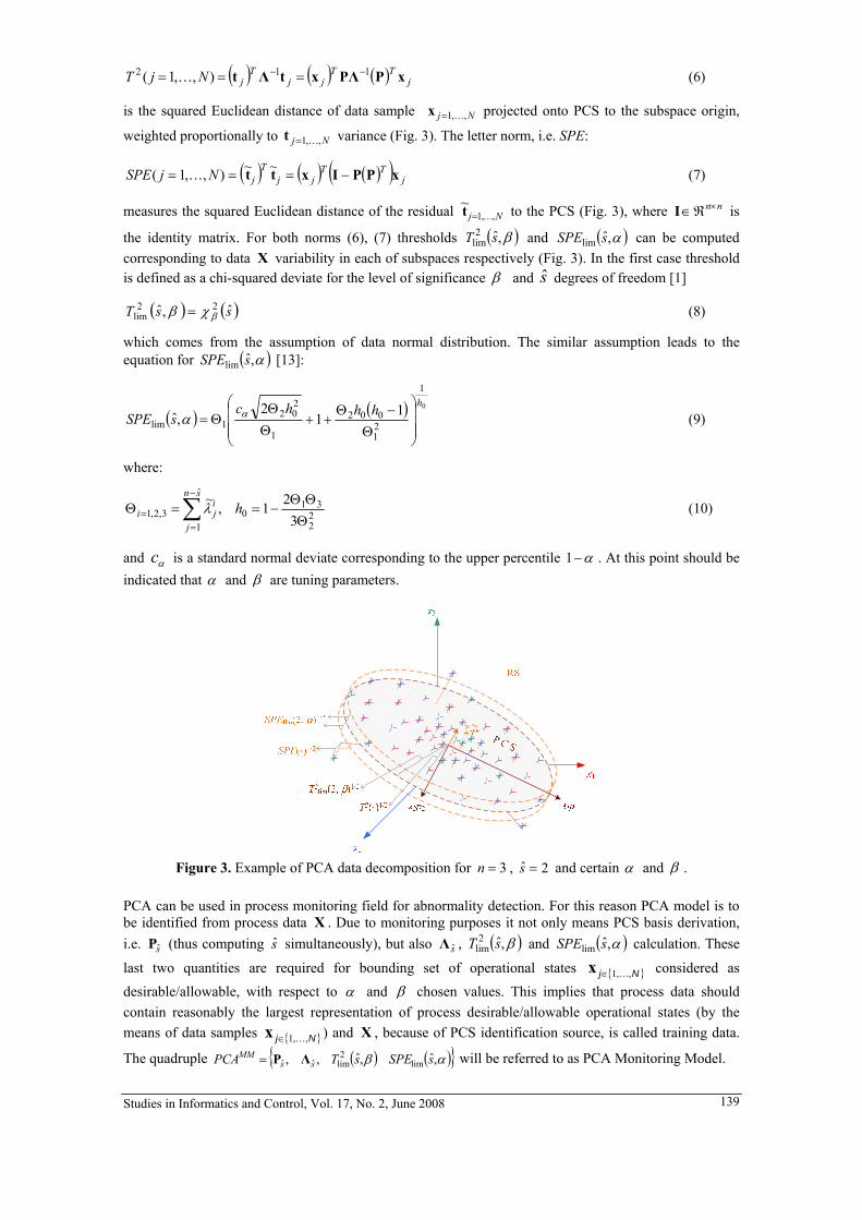
( ) ( ) ( ) jTT
jjT
jNjT xPPΛxtΛt 112 ),,1( −− === K (6)
is the squared Euclidean distance of data sample projected onto PCS to the subspace origin,
weighted proportionally to variance (Fig. 3). The letter norm, i.e. SPE: Nj ,,1K=x
Nj ,,1K=t
( ) ( ) ( )( jTT
jjT
jNjSPE xPPIxtt −=== )~~),,1( K (7)
measures the squared Euclidean distance of the residual Nj ,,1~
K=t to the PCS (Fig. 3), where is
the identity matrix. For both norms (6), (7) thresholds
nn×ℜ∈I
( )β,ˆ2lim sT and ( )α,ˆlim sSPE can be computed
corresponding to data variability in each of subspaces respectively (Fig. 3). In the first case threshold is defined as a chi-squared deviate for the level of significance
Χβ and degrees of freedom [1] s
( ) (ssT ˆ,ˆ 22lim βχβ = )
)
(8)
which comes from the assumption of data normal distribution. The similar assumption leads to the equation for ( α,ˆlim sSPE [13]:
( ) ( ) 0
1
21
002
1
202
1lim11
2,ˆ
hhhhcsSPE
⎟⎟⎟
⎠
⎞
⎜⎜⎜
⎝
⎛
Θ−Θ
++ΘΘ
Θ= αα (9)
where:
22
310
ˆ
13,2,1 3
21,~ΘΘΘ
−==Θ ∑−
== h
sn
j
iji λ (10)
and is a standard normal deviate corresponding to the upper percentile αc α−1 . At this point should be indicated that α and β are tuning parameters.
Figure 3. Example of PCA data decomposition for 3=n , 2ˆ =s and certain α and β .
PCA can be used in process monitoring field for abnormality detection. For this reason PCA model is to be identified from process data . Due to monitoring purposes it not only means PCS basis derivation, i.e. (thus computing simultaneously), but also ,
Χ
sP s sΛ ( )2 β,ˆlim sT and ( )α,ˆlim sSPE calculation. These
last two quantities are required for bounding set of operational states considered as desirable/allowable, with respect to
{ Nj ,,1K∈ }xα and β chosen values. This implies that process data should
contain reasonably the largest representation of process desirable/allowable operational states (by the means of data samples ) and , because of PCS identification source, is called training data.
The quadruple { }j ,1K∈x ΧN,
( ){ ( )}α,ˆ,, 2 ssTPCA ssMM ΛP= β,ˆ limlimˆˆ SPE will be referred to as PCA Monitoring Model.
Studies in Informatics and Control, Vol. 17, No. 2, June 2008 139
After is obtained off-line from training data, the next step is the actual process monitoring performed on-line for data samples constructed analogously to . Since corresponds to
the model of the process under monitoring, current norms values :
MMPCA( )kx Nj ,,1K=x sP
)(2 kT
( )( ) ( ) (kkkT Tss
T xPΛPx s1
ˆˆ2 )( −= ) (11)
and : )(kSPE
( )( ) ( )( ) ( )kkkSPE Tss
T xPPIx ˆˆ)( −= (12)
measure the (quadratic) distances of current operational state from their, training data based, expected values. Thus ratios ( ) ( β,ˆ/ 2
lim2 sTkT ) and ( ) ( )α,ˆ/ lim sSPEkSPE can be used for abnormal operational state
indication/detection in case of unity violation by either of them:
( )( )
( )( ) 1
,ˆ1
,ˆ:instatnt at time state opertional abnormal
lim2
lim
2>∨>
αβ sSPEkSPE
sTkTk (13)
and the indication/detection magnitude (values of ratios ( ) ( )β,ˆ/ 2lim
2 sTkT and ( ) ( )α,ˆ/ lim sSPEkSPE ) depends on the abnormality magnitude measured by the (11), (12) relatively to the closest operational state concerned as a desirable/allowable, represented by the thresholds (7), (8).
As far as the monitored process fulfil PCA assumptions, there is a fundamental difference between abnormality detection by the and ( ) ( β,ˆ/ 2
lim2 sTkT ) ( ) ( )α,ˆ/ lim sSPEkSPE ratios. The former value indicates abnormal
operational states, which preserve cross-correlation structure of the process, hence caused mainly by the operation point changes, while the latter ratio is responsible for abnormalities detection of PCA modelled process. However in case of nonlinear process under PCA monitoring, which can be often found in practice [5], [6], [14] – [19], since PCS contains only linearised and originally linear part of dependencies among variables , current values indicate an abnormality being a mixture of operation
point as well as whole process changes, both not perpendicular to the directions. The same applies to the second ratio
Nj ,,1K=x ( ) ( β,ˆ/ 2lim
2 sTkT )
)sP
( ) ( α,ˆ/ lim sSPEkSPE , with an exception, that this measure detects abnormal operational states (again a mixture of operation point and process changes) not captured by the PCS.
3. MultiRegional Principal Component Analysis
Distributed Systems (DSs) can be decomposed into regions such that operational state of DS follow this decomposition resulting in a set of local (regional) operational states. Because DSs posses network process structure, any local operational state is mutually dependant of its neighbouring regions, where the dependencies are defined by network topology. Hence any source of a abnormal operational state of DS can be analysed through the local operational states, which indicate a local abnormality, if and only if, the abnormality in question, has significant influence on them (local operational states). Significance of analysed abnormality is given by some measure of desirability/allowability of operational state.
Moreover, it is the network topology that defines, which of local models (representing local operational states) are sensitive to abnormal operational state of DS with respect to its particularly placed source. This knowledge can be used to establish a methodology for abnormality source localization.
In case of PCA chosen as a basis monitoring method, as many regions of DS should be distinguished as it is possible, subject to -th region compactness and minimal number of monitored variables
. For each of regions a local (regional) PCA Monitoring Model and
Rj 1>jn
jj nix ,,1K= R MMRjPCA ,,1K=
( ) ( ){ }jjjjjjjsjsMMj sSPEsTPCA
jjαβ ,ˆ,,ˆ,, lim,
2lim,,ˆ,ˆ ΛP= is to be derived following the methodology
stated in the previous section (2.1). Defining norms for the -th region j ( )kTj2 and analogously
to (11), (12) computed at time instant with respect to local data sample , ratios:
and
( )kSPEj
k ( ) jnj k ℜ∈x
( ) ( jjjj sTkT β,ˆ/ 2lim,
2 ) ( ) ( )jjjj sSPEkSPE α,ˆ/ lim, are considered as measures of desirability/allowability
Studies in Informatics and Control, Vol. 17, No. 2, June 2008 140

of local operational state and again (13) it assumed, that for the -th region if either of these ratios violates unity, there is an abnormality in DS causing local abnormal operational state. Thus abnormal operational states indication by particular local models still depends on its magnitude (relatively to the closest operational state concerned as a desirable/allowable), however in this case abnormality magnitude is understood locally, i.e. corresponds to particular regional PCA Monitoring Model.
j
It is important to notice, that it is possible to distinguish between ‘process’ abnormality of DS and a sensor fault. While the latter is detected only by one regional PCA Monitoring Model (assigned to the specific sensor), the abnormality of DS radiates into all regions causing changes in and ( )kT j
2 ( )kSPEj in more then one adjacent PCA Monitoring Model.
Network process structure of DSs can be illustrated by the means of nodes and links, which connections structure follows the network topology. From this point of view any distinguished region should consist of variables measured at a node and in all connected links. In special case of isotropic topology (Fig. 4) the highest desirable/allowable regional operational state violation, thus also the highest abnormality indication, is in the neighbourhood of abnormality source, since the grater is the distance of local model from the abnormality source localization, the less its operational state depends on abnormality ‘injected’ into the network.
Process abnormality
Max
imum
T2 a
nd S
PE
at t
ime
inst
ant k
Ti2(k) and SPEi(k)
exceeded threshold
Tj2(k) and SPEj(k)
under threshold
Figure 4. Visualisation of MR-PCA approach
Detection and localisation of abnormality source in DS can be briefly described as follows:
1. During the process operation both measures ( )kT j2 and ( )kSPEj for all regional PCA
Monitoring Models are monitored. R
2. If any measure exceeds corresponding threshold ( )jjj sT β,ˆ2lim, or ( )jjj sSPE α,ˆlim, respectively,
then it is said that a certain abnormality (including sensor faults) occurs.
3. If it is only one regional PCA Monitoring Model that indicate abnormality, first check for sensor fault among locally measured variables . Else, at once consider detected abnormality
as affecting the process. jn
jj nix ,,1K=
4. Regional PCA Monitoring Models with the largest ( ) ( jjjj sTkT β,ˆ/ 2lim,
2 ) or
( ) ( )jjjj sSPEkSPE α,ˆ/ lim, values determine the localisation of the process abnormality source.
The main idea of proposed method is quite similar to Multi Block Principal Component Analysis (MB-PCA) presented in [20]. However, this name appeared earlier and was dedicated for quite different approach [21]. Therefore, it was proposed [5], [6] to name the method MultiRegional PCA (MR-PCA).
4. Drinking Water Distribution Systems
Drinking Water Distribution System (DWDS) is a good example of a DS. In this section the general description of DWDS is presented.
Nowadays, DWDS is one of the most important systems in community. Its efficient control requires advanced
Studies in Informatics and Control, Vol. 17, No. 2, June 2008 141

method e.g. predictive control [22], [23] or adaptive control and reliable monitoring system. Proposed approach is applied to detection and localisation of failures in DWDS. Usually in DWDS, drinking water is introduced into the network by using pumps (pumping station) and transported through the network by pipes. Pipes connect in nodes where delivered water is mixed and transported farther. Flows through the pipes are enforced by nodal pressure differences. These are caused by pumps or/and by the water tanks. Tanks are used to store the water in periods when water production is greater then its consumption [23].
The network mathematical model is composed of two parts: static and dynamic. The static part is typically available in an implicit form represented by the element algebraic equalities and the interconnection equalities. This is described for water networks by Brdys and Ulanicki [25]. In general, the element algebraic equalities are described by non-linear functions. The interconnection equalities can be written based on conservation equations. Using the energy loss-gain relationships for the different elements of water distribution system, the conservation equation can be written in three forms: the node, the loop and pipe equations [26].
Unlike the node and loop equations, the pipe equations are solved for the vector of pipe flows Q and hydraulic head h simultaneously. Formulating the static part of water distribution network mathematical model we use the pipe form. The dynamic part of the network mathematical model is represented by differential equalities describing tanks. Because the measurements are available at discrete moments, the water distribution network model is formulated in discrete form.
Paper considers detection and localization of water pipe leakages. The DWDS is modelled in simulation packages Epanet [27]. The leakages are modelled as an emitter. The flow rate through the emitter varies as a function of pressure available at the node [27]:
γpCQ = (14)
where: Q is the flow rate, p is the pressure and C is the discharge coefficient (emitter coefficient), finally γ is the pressure exponent.
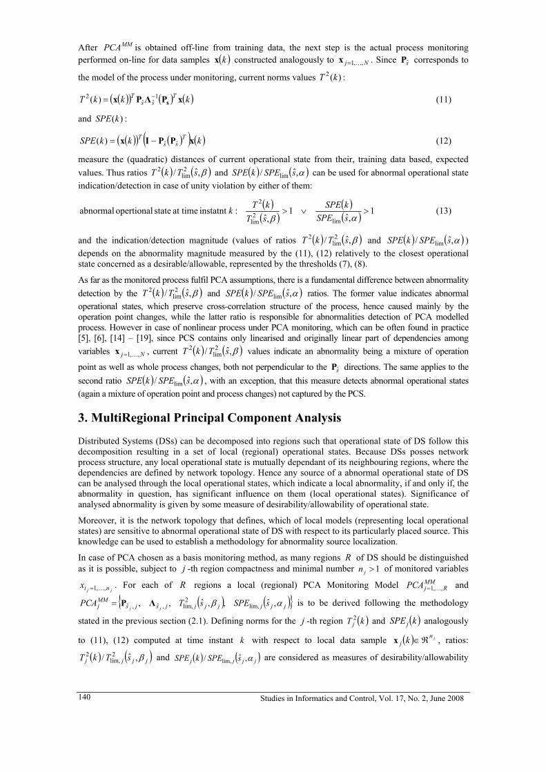
5. MultiRegional Principal Component Analysis in Application to Drinking Water Distribution Systems
Most often faults in DWDS are pump breakdowns and water leakages from the pipes. The former is easy to identify while the leakage detection and localisation is harder as it is placed underground. The faults might be detected based on the system measurements.
When diagnosis of DWDS is under the consideration monitoring and diagnostics methods are directly divided into two groups [4]: ‘measurements and model based’, e.g. Inverse Transient Method [2] and ‘measurements based’ [7], [10], [11]. A group of measurement based methods utilizes statistical data analysis [28], but these methods are still in the stage of research and development [4]. Moreover available active leakage control methods are basically unpractical due to costs and time consuming or having the long leak detection and location times [4]. This is not the case of MR-PCA, which can join not only relatively uncomplicated statistical analysis dedicated to DSs, such as DWDS (due to SD) but also experience of staff working in water companies. Moreover, this method compromises between detection and localisation efficiency and a number of measuring devices [5], [6].
In the DWDS one can measure the water pipe flows, pressure in the nodes, water level in the tanks and water quality (e.g. chlorine concentration). For DWDS approach region (when regional PCA Monitoring Models are taken into consideration) means a measurement nodes together with all adjacent links, while the abnormal DWDS operational state is said to be caused by the single water leakage.
5.1 Fundamentals
Local -th PCA Monitoring Model for each of regions consists of the locally identified PCS basis
with corresponding modelled variance information in diagonal matrix , as well as thresholds
computed for local abnormality indication. All these elements are derived with respect to chosen PCS dimensionality (e.g. using CPV criteria (4), (5), thus also ) and
j MMjPCA R
js j ,ˆP js j ,ˆΛ
js jCPVlim, jα , jβ parameters.
Local PCA models use nodal heads (heads is a sum of nodal pressure and its geodetic heights) and adjacent pipe flows as process variables (of course for PCA models identification as well as on-line
Studies in Informatics and Control, Vol. 17, No. 2, June 2008 142

DWDS regions monitoring). Since each local model (PCA model or PCA Monitoring Model) in all cases includes one quantity connected to a particular node (namely nodal head), the ‘Identification number’ of the particular node will be referred to as the model name and replaces its -th index. It means, e.g. (Fig.
5) that PCA Monitoring Model is related to the head in the node ‘88’ and flows in the pipes linking this particular node with its neighbours, which are: ‘44’, ‘55’ and ‘66’.
jMMPCA '88'
The minimal percent of variance captured by the -th PCA model, , in all cases is set to 95%. However due to existing nonlinearities this ensures only capture of the linearization results by PCS. Values
j jCPVlim,
jα and jβ are selected separately to ensure abnormality detection (with respect to given local PCA model) and simultaneously false alarms reduction. This implies in the non-normal and nonlinear case of the DWDS, that one must pay special attention while tuning jα and jβ . Authors in most of further presented
case studies assigned values from the range 7,06,0 ÷ and 9,07,0 ÷ for jα and jβ respectively.
5.2 Simple water network case study
Paper presents MR-PCA method in application to leakage detection in Chojnice drinking water distribution network. Large numbers of potential leakages in the network as well as potential monitoring points might be investigated, there. Hence in order to explain the fundamentals of the method and to illustrate well its efficiency, the simulations were carried out on small testing network (Fig. 5), where the leakages were modelled in different but very meaningful places, as an extra node with pressure dependent demand (Emitter).
Fig. 5 presents three case studies when the leakage was modelled in different places in the testing network. First leakage was modelled in pipe between nodes ‘44’ and ‘88’ (Section 5.2.1), the second one in pipe between nodes ‘29’ and ‘30’ (Section 5.2.2) and the last one in pipe between nodes ‘25’ and ‘28’ (Section 5.2.3). All leakages took place between 46th and 52th hour.
Leakage 144
22 55
6688
31 3029
32
28
2526
27
Leakage 2
Leakage 3
Figure 5. Simple water network. Modelled leakages marked with blue dots
The following figures present the effects of monitoring process by using PCA Monitoring Models designed based on flow rates delivering water to particular node and its nodal head.
5.2.1 Water main screening effect
The dashed blue lines in Fig. 6. represents results of quality measures T2 and SPE simulated on the training data, without any leakage. The solid red lines represents an effect of monitoring for the same simulation period but with modelled leakage (in pipe between nodes ‘44’ and ‘88’).
Studies in Informatics and Control, Vol. 17, No. 2, June 2008 143
MMPCA '22' 0
0.5
1
T2 /T2 lim
[-]
40 45 50 55 600
50
100
t [h]
SP
E/S
PE
lim [-
] MMPCA '44' 0
0.5
1
T2 /T2 lim
[-]
40 45 50 55 600
50
100
t [h]
SP
E/S
PE
lim [-
]
MMPCA '55'
11
0
0.5
T2 /T2 lim
[-]
40 45 50 55 600
20
40
t [h]
SP
E/S
PE
lim [-
] MMPCA '66' 0
T2 /T2 lim
[-]
0.5
10
40 45 50 55 600
5
t [h]
SP
E/S
PE
lim [-
]
MMPCA '88'
11
0
0.5
T2 /T2 lim
[-]
40 45 50 55 600
20
40
t [h]
SP
E/S
PE
lim [-
] MMPCA '31' 0
T2 /T2 lim
[-]
0.5
1
40 45 50 55 600
0.5
t [h]
SP
E/S
PE
lim [-
]
Figure 6. Leakage monitoring results by PCAMM designed at selected nodes – water main screening effect (simulation without leakage (training) - blue; simulation with modelled leakage – red)
Differences between the lines representing PCA models being identified on training data and its current (simulated) responses indicate that something unusual has took place in the network. In this particular example it means pipe water leakage. Notice how considerable increase of the T2 and SPE measures is generated by PCA Monitoring Models ‘44’, ‘22’, ‘66’ and ‘88’ ( ; ;MM MMPCA '44' PCA '22' '66'
MM
MM
MM
)
PCA and
). It simply means that the leakage has significantly disturbed the water flow rates and pressures
being the base for particular PCA Monitoring Models (PCA
PCA '88'
MM). There are also PCAMM e.g. that do not indicate any abnormalities in the network in spite being in similar distance to the leakage. Such a phenomenon is rather strange at the first glance. However, these models are designed based on measurements gathered from points laying ‘behind’ the water main. Hence, the significant amount of water flowing by the water main causes that modelled leakage did not significantly affect the usual (operating states represented by training data) flow rates and nodal heads on the other side of water main. This implies that the PCA Monitoring Models are unable to detect the leakage. In the paper such an effect is called ‘screening effect’ of the water main.
PCA '31'
5.2.2 Water tank screening effect
This section presents a case when the leakage was modelled in pipe between nodes ‘29’ and ‘30’. Similarly to the previous case study some of the PCA Monitoring Models produce quality measures significantly exceeding the assumed threshold (unity in the case of ratios and ( ) ( jjjj sTkT β,ˆ/ 2
lim,2
( ) ( )jjjj sSPEkSPE α,ˆ/ lim, monitoring) e.g. ; ; , and , what indicates the leakage (Fig. 7). In opposite, there are models that generate measures similar to their training values what suggests that noting unusual happened.
MMPCA '55'MMPCA '28'
MMPCA '29'MMPCA '31'
MMPCA '32'
Studies in Informatics and Control, Vol. 17, No. 2, June 2008 144
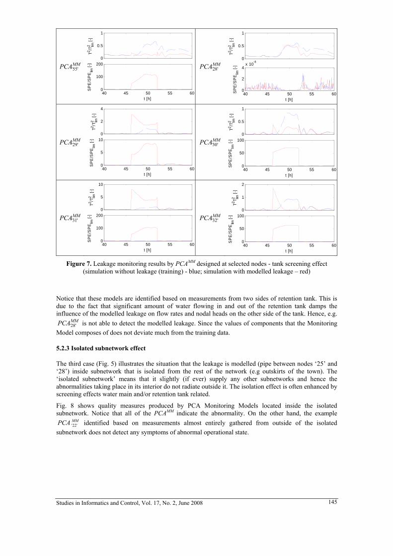
MM''PCA55
0
0.5
1
T2 /T2 lim
[-]
40 45 50 55 600
100
200
t [h]
SP
E/S
PE
lim [-
] MMPCA '28'
0
0.5
1
T2 /T2 lim
[-]
40 45 50 55 600
2
4x 10⁻⁸
t [h]
SP
E/S
PE
lim [-
]
MMPCA '29'
14
0
2
T2 /T2 lim
[-]
40 45 50 55 600
5
10
t [h]
SP
E/S
PE
lim [-
] MMPCA '30'
0
T2 /T2 lim
[-]
0.5
100
40 45 50 55 600
50
t [h]
SP
E/S
PE
lim [-
]
MMPCA '31'
10 2
0
5
T2 /T2 lim
[-]
40 45 50 55 600
100
200
t [h]
SP
E/S
PE
lim [-
] MMPCA '32'
0
T2 T2 lim [-
]
1
100
40 45 50 55 600
50
t [h]
SP
E/S
PE
lim [-
]
Figure 7. Leakage monitoring results by PCAMM designed at selected nodes - tank screening effect (simulation without leakage (training) - blue; simulation with modelled leakage – red)
Notice that these models are identified based on measurements from two sides of retention tank. This is due to the fact that significant amount of water flowing in and out of the retention tank damps the influence of the modelled leakage on flow rates and nodal heads on the other side of the tank. Hence, e.g.
is not able to detect the modelled leakage. Since the values of components that the Monitoring Model composes of does not deviate much from the training data.
MMPCA '28'
5.2.3 Isolated subnetwork effect
The third case (Fig. 5) illustrates the situation that the leakage is modelled (pipe between nodes ‘25’ and ‘28’) inside subnetwork that is isolated from the rest of the network (e.g outskirts of the town). The ‘isolated subnetwork’ means that it slightly (if ever) supply any other subnetworks and hence the abnormalities taking place in its interior do not radiate outside it. The isolation effect is often enhanced by screening effects water main and/or retention tank related.
Fig. 8 shows quality measures produced by PCA Monitoring Models located inside the isolated subnetwork. Notice that all of the PCAMM indicate the abnormality. On the other hand, the example
identified based on measurements almost entirely gathered from outside of the isolated subnetwork does not detect any symptoms of abnormal operational state.
MMPCA '22'
Studies in Informatics and Control, Vol. 17, No. 2, June 2008 145

MMPCA '55' 0
0.5
1
T2 /T2 lim
[-]
40 45 50 55 600
50
100
t [h]
SP
E/S
PE
lim [-
] MMPCA '25'
0
10
20
T2 /T2 lim
[-]
40 45 50 55 600
200
400
t [h]
SP
E/S
PE
lim [-
]
MMPCA '26'
1010
0
5
T2 /T2 lim
[-]
40 45 50 55 600
200
400
t [h]
SP
E/S
PE
lim [-
] MMPCA '27'
0
T2 /T2 lim
[-]
5
400
40 45 50 55 600
200
t [h]
SP
E/S
PE
lim [-
]
MMPCA '28'
2 1
0
1
T2 /T2 lim
[-]
40 45 50 55 600
5
10x 10
5
t [h]
SP
E/S
PE
lim [-
] MMPCA '22'
0
T2 /T2 lim
[-]
0.5
1
40 45 50 55 600
0.5
t [h]
SP
E/S
PE
lim [-
]
Figure 8. Leakage monitoring results by PCAMM designed at selected nodes – isolated region effect (simulation without leakage (training) - blue; simulation with modelled leakage – red)
5.2.4 Distinguishing the subnetworks
Screening effects of the water mains, water tanks and isolated subnetwork are the serious disadvantage in leakage detection and localisation process at the first glance. However, skilfully utilisation of these features allows for improving the efficiency of faults monitoring process. Possessing the knowledge about DWDS characteristics (pipe flow rates, velocities, nodal heads, diameters of pipes, tank localisations etc.) one can divide the network into several independent subnetworks. The subnetworks should be selected in such a way to enable for independent (with respect to abnormalities significance indication) leakage detection inside them. Such an approach enables for placing much less measuring devices for detecting and then localising the leakages. As the results number of simulations and confronting them with network topology, three regional subnetworks have been distinguished (Fig. 9).
44
22 55
6688
31 3029
32
28
2526
27
Figure 9. Selecting the regional subnetworks within the simple network
Another step after the detection of the leakage is its localization. It is clearly seen that there is strong correlation between values of both quality measures and distance from leakage and PCA Monitoring Model (Fig. 6, 7 and 8). Namely, in case of leakage the highest values of T2 and SPE are produced by
Studies in Informatics and Control, Vol. 17, No. 2, June 2008 146
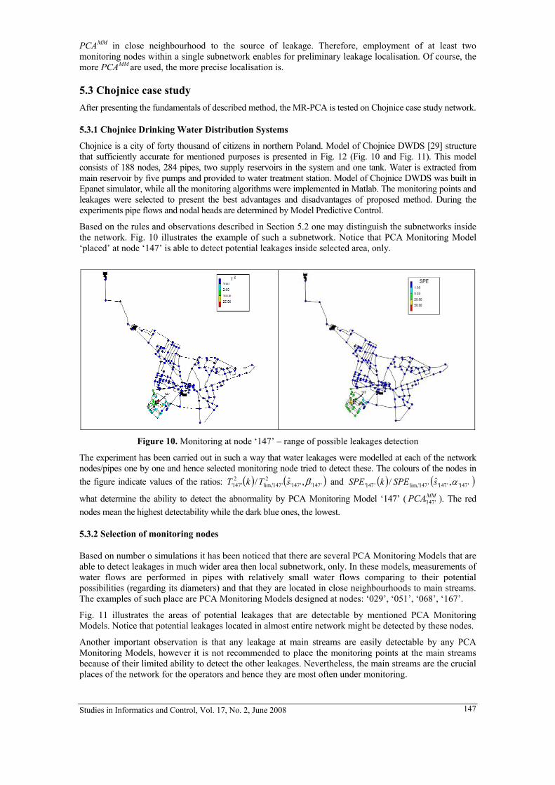
PCAMM in close neighbourhood to the source of leakage. Therefore, employment of at least two monitoring nodes within a single subnetwork enables for preliminary leakage localisation. Of course, the more PCAMM are used, the more precise localisation is.
5.3 Chojnice case study After presenting the fundamentals of described method, the MR-PCA is tested on Chojnice case study network.
5.3.1 Chojnice Drinking Water Distribution Systems
Chojnice is a city of forty thousand of citizens in northern Poland. Model of Chojnice DWDS [29] structure that sufficiently accurate for mentioned purposes is presented in Fig. 12 (Fig. 10 and Fig. 11). This model consists of 188 nodes, 284 pipes, two supply reservoirs in the system and one tank. Water is extracted from main reservoir by five pumps and provided to water treatment station. Model of Chojnice DWDS was built in Epanet simulator, while all the monitoring algorithms were implemented in Matlab. The monitoring points and leakages were selected to present the best advantages and disadvantages of proposed method. During the experiments pipe flows and nodal heads are determined by Model Predictive Control.
Based on the rules and observations described in Section 5.2 one may distinguish the subnetworks inside the network. Fig. 10 illustrates the example of such a subnetwork. Notice that PCA Monitoring Model ‘placed’ at node ‘147’ is able to detect potential leakages inside selected area, only.
Figure 10. Monitoring at node ‘147’ – range of possible leakages detection
The experiment has been carried out in such a way that water leakages were modelled at each of the network nodes/pipes one by one and hence selected monitoring node tried to detect these. The colours of the nodes in the figure indicate values of the ratios: ( ) ( )'147''147'
2'147'lim,
2'147' ,ˆ/ βsTkT and ( ) ( )'147''147''147'lim,'147' ,ˆ/ αsSPEkSPE
what determine the ability to detect the abnormality by PCA Monitoring Model ‘147’ ( ). The red nodes mean the highest detectability while the dark blue ones, the lowest.
MMPCA '147'
5.3.2 Selection of monitoring nodes
Based on number o simulations it has been noticed that there are several PCA Monitoring Models that are able to detect leakages in much wider area then local subnetwork, only. In these models, measurements of water flows are performed in pipes with relatively small water flows comparing to their potential possibilities (regarding its diameters) and that they are located in close neighbourhoods to main streams. The examples of such place are PCA Monitoring Models designed at nodes: ‘029’, ‘051’, ‘068’, ‘167’.
Fig. 11 illustrates the areas of potential leakages that are detectable by mentioned PCA Monitoring Models. Notice that potential leakages located in almost entire network might be detected by these nodes.
Another important observation is that any leakage at main streams are easily detectable by any PCA Monitoring Models, however it is not recommended to place the monitoring points at the main streams because of their limited ability to detect the other leakages. Nevertheless, the main streams are the crucial places of the network for the operators and hence they are most often under monitoring.
Studies in Informatics and Control, Vol. 17, No. 2, June 2008 147

MMPCA '68'
MMPCA '29'
Figure 11. The leakages detectability by PCA Monitoring Models designed at nodes ‘068’ and ‘029’
In the result of such an analysis five subnetworks has been selected for Chojnice network and two monitoring places at of the regions have been indicated. These are presented at Fig. 12.
PCA Monitoring Models
subnetworks
Retention tanks
Pipes
Pumps
Nodes
Figure 12. The Chojnice DWDS. Green ellipsoids mark the selected subnetworks while blue dots mark
assumed PCA Monitoring Models.
5.3.3 Simulation results - leakage detection and localization
Fig. 13 presents the results of monitoring the Chojnice DWDS by PCA Monitoring Models designed at nodes marked in Fig. 12. The situation without leakage (training data) is marked blue lines in the figures, while simulations with modelled leakage are marked red. Simulations show that only PCA Monitoring Models build at nodes ‘152’ and ‘144’ unambiguously have indicated the failure (both SPE and T2 have significantly exceeded the thresholds). These models consist of nodal heads and pipe flows measurements gathered inside one selected subnetwork, namely ‘IV’ (Fig. 12). It leads to conclusions that simulated leakage is located within this area. Moreover, SPE and T2 produced by are much greater then measures of , hence it might suggests that the abnormality took place closer to the node ‘152’ (and it indeed is in this case), however one cannot treat this as a straight rule without taking into account the network topology and actual water distributions and its ‘trace’. Example of tool enable for analysing the routes of water flowing inside the network is an algorithm making possible for water paths (routes) finding [30].
MMPCA '152'MMPCA '144'
Besides of and , also PCA Monitoring Model ‘029’ indicates the leakage by its TMMPCA '152'MMPCA '144'
2 measure but as mentioned earlier it is the model of special sensitivity.
Studies in Informatics and Control, Vol. 17, No. 2, June 2008 148

MMPCA '36' 0
0.5
T2 /T2 lim
[-]
50 55 60 65 700
0.5
x 10-14
SP
E/S
PE
lim [-
]
t [h]
MMPCA '29'
0
2
4
T2 /T2 lim
[-]
50 55 60 65 700
1
2x 10⁻³
SP
E/S
PE
lim [-
]
t [h]
MMPCA '44'
1 0.5
0
T2 /T2 lim
[-]
T2 /T2 lim
[-]
0.5
0
50 55 60 65 700
0.5
1x 10
-3
SP
E/S
PE
lim [-
]
t [h]
MMPCA '123'
50 55 60 65
0.5
x 10-14
700S
PE
/SP
Elim
[-]
t [h]
MMPCA '170
0.5 0.5
T2 /T2 lim
[-]
T2 /T2 lim
[-]
0 0
50 55 60 65 700
1
2x 10
-31
SP
E/S
PE
lim [-
]
t [h]
MMPCA '137'
50 55 60 65
1x 10⁻⁵
700
0.5S
PE
/SP
Elim
[-]
t [h]
MMPCA '152'
24000
0
2000
T2 /T2 lim
[-]
50 55 60 65 700
5000
10000
SP
E/S
PE
lim
t [h]
[-] MMPCA '144'
0
T2 /T2 lim
[-]
1
0.2
50 55 60 65 700
0.1
SP
E/S
PE
lim [-
]
t [h]
Figure 13. Leakage monitoring results by PCA Monitoring Models designed at selected nodes (simulation without leakage (training) - blue; simulation with modelled leakage – red)
Figure 14. Fragment of the Chojnice network with broken water pipe flow sensor in pipe ‘152’
Studies in Informatics and Control, Vol. 17, No. 2, June 2008 149
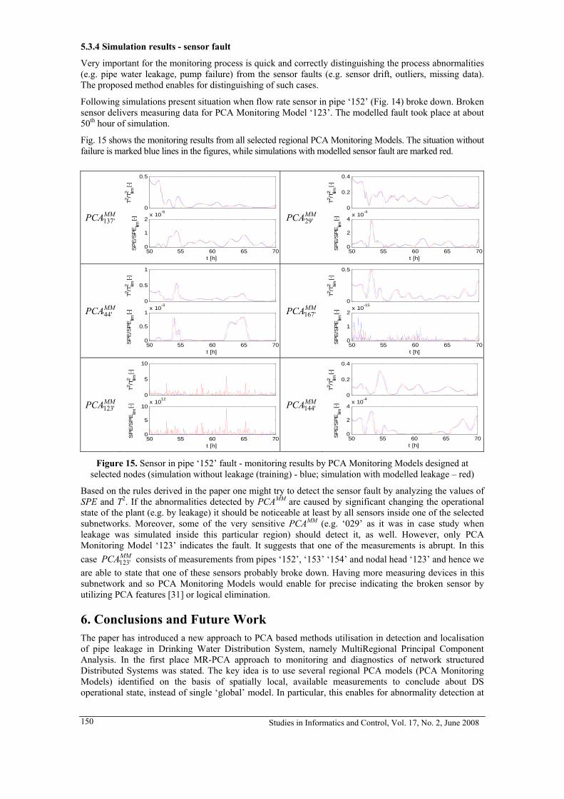
5.3.4 Simulation results - sensor fault
Very important for the monitoring process is quick and correctly distinguishing the process abnormalities (e.g. pipe water leakage, pump failure) from the sensor faults (e.g. sensor drift, outliers, missing data). The proposed method enables for distinguishing of such cases.
Following simulations present situation when flow rate sensor in pipe ‘152’ (Fig. 14) broke down. Broken sensor delivers measuring data for PCA Monitoring Model ‘123’. The modelled fault took place at about 50th hour of simulation.
Fig. 15 shows the monitoring results from all selected regional PCA Monitoring Models. The situation without failure is marked blue lines in the figures, while simulations with modelled sensor fault are marked red.
MMPCA '137' 0
0.5
T2 /T2 lim
[-]
50 55 60 65 700
1
2x 10⁻⁶
SP
E/S
PE
lim [-
]
t [h]
MMPCA '29'
0
0.2
0.4
T2 /T2 lim
[-]
50 55 60 65 700
2
4x 10⁻⁴
SP
E/S
PE
lim [-
]
t [h]
MMPCA '44'
1 0.5
0
T2 /T2 lim
[-]
T2 /T2 lim
[-]
0.5
0
50 55 60 65 700
0.5
1x 10⁻³
SP
E/S
PE
lim [-
]
t [h]
MMPCA '167'
50 55 60 65
2x 10-15
700
1
SP
E/S
PE
lim [-
]
t [h]
MMPCA '123'
10 0.4
0
5
T2 /T2 lim
[-]
50 55 60 65 700
5
10x 10
12
SP
E/S
PE
lim [-
]
t [h]
MMPCA '144'
0
T2 /T2 lim
[-]
0.2
50 55 60 65
4x 10⁻⁴
700
2
SP
E/S
PE
lim [-
]
t [h]
Figure 15. Sensor in pipe ‘152’ fault - monitoring results by PCA Monitoring Models designed at selected nodes (simulation without leakage (training) - blue; simulation with modelled leakage – red)
Based on the rules derived in the paper one might try to detect the sensor fault by analyzing the values of SPE and T2. If the abnormalities detected by PCAMM are caused by significant changing the operational state of the plant (e.g. by leakage) it should be noticeable at least by all sensors inside one of the selected subnetworks. Moreover, some of the very sensitive PCAMM (e.g. ‘029’ as it was in case study when leakage was simulated inside this particular region) should detect it, as well. However, only PCA Monitoring Model ‘123’ indicates the fault. It suggests that one of the measurements is abrupt. In this case consists of measurements from pipes ‘152’, ‘153’ ‘154’ and nodal head ‘123’ and hence we are able to state that one of these sensors probably broke down. Having more measuring devices in this subnetwork and so PCA Monitoring Models would enable for precise indicating the broken sensor by utilizing PCA features [31] or logical elimination.
MMPCA '123'
6. Conclusions and Future Work The paper has introduced a new approach to PCA based methods utilisation in detection and localisation of pipe leakage in Drinking Water Distribution System, namely MultiRegional Principal Component Analysis. In the first place MR-PCA approach to monitoring and diagnostics of network structured Distributed Systems was stated. The key idea is to use several regional PCA models (PCA Monitoring Models) identified on the basis of spatially local, available measurements to conclude about DS operational state, instead of single ‘global’ model. In particular, this enables for abnormality detection at
Studies in Informatics and Control, Vol. 17, No. 2, June 2008 150
least. Moreover the network topology of DS may be imbedded into the MR-PCA structure resulting in better diagnostic capabilities.
Since DWDS is a representative of network systems, its abnormal operational states detection and identification can be realised by MR-PCA. In the paper pipe leakages are assumed to be the only one process abnormalities. MR-PCA methodology illustrating simulations ware presented on a simple example of water network first. These, performed for a number of demand scenarios, confirmed the ability of MR-PCA to conduct the system diagnosis with regard to leakages detection and localisation. Furthermore additional phenomena were observed, providing abnormalities localisation complexity to be reduced, due to DWDS subnetworks distinguishing criteria. These are water main and retention tank screening effects, as well as isolated subnetwork effect. In practice only small part of the network variables can be directly measured. However, this does not constrain MR-PCA capabilities of leakages detection and localisation, as long as one is able to ensure at least two local PCA Monitoring Models per distinguished DWDS subnetwork, placed in their certain regions. Choice of these regions, i.e. DWDS sensors allocation is suggested from the MR-PCA abnormalities detectability point of view. Obtained results were successfully applied to case study DWDS Chojnice (Northern Poland).
At this state of the research the accurate localisation of the leakages is supervised by a man. In the future the neural networks and/or fuzzy clustering will be used to complete the process of automatic abnormalities localisation. Moreover, MR-PCA will be a part of supervised Fault Tolerant Model Predictive Control. Another subject of research in the field of fault detection and localisation will focus on identifying the process abnormality type e.g. pipe leakage, pump or valve breakdown. Obtained results are promising and have rather generic nature, hence might be transferred into other DSs e.g. pipeline systems, telecommunication systems, power systems etc, known as a network systems.
REFERENCES
1. JACKSON, J.E., A User's Guide to Principal Components, Wiley-Interscience (New York), 1991.
2. VÍTKOVSKÝ, J.P., SIMPSON, A.R. and LAMBERT, M.F., Leak Detection and Calibration Using Transients and Genetic Algorithms, J. Water Resour. Plng. and Mgmt 126, 2000.
3. POULAKIS, Z., VALOUGEORGIS, D. and PAPADIMITRIOU, C., Leakage Detection in Water Pipe Networks Using a Bayesian Probabilistic Framework, Probabilistic Engineering Mechanics 18, 2003.
4. MISIUNAS, D., Failure Monitoring and Asset Condition Assessment in Water Supply Systems. Ph.D thesis, Department of Industrial Electrical Engineering and Automation, Lund University (Lund), 2005.
5. BOROWA, A., MAZUR, K., GROCHOWSKI, M., BRDYŚ, M.A. and JEZIOR, K., MultiRegional PCA for Leakage Detection and Localisation in DWDS – Approach, (Eds.) KORBICZ J., PATAN K. and KOWAL M., Fault Diagnosis and Fault Tolerant Control, Academic Publishing House EXIT (Warsaw), 2007.
6. JEZIOR, K., MAZUR, K., BOROWA, A., GROCHOWSKI, M. and BRDYS, M.A., MultiRegional PCA for Leakage Detection and Localisation in DWDS – Chojnice Case Study, (Eds.) KORBICZ J., PATAN K. and KOWAL M., Fault Diagnosis and Fault Tolerant Control, Academic Publishing House EXIT (Warsaw), 2007.
7. VENKATASUBRAMANIAN, V., RENGASWAMY, R., KAVURI, S.N. and YIN, K., A Review of Process Fault Detection and Diagnosis Part III: Process History Based Methods, Computers and Chemical Engineering 27, 2003.
8. ZHANG, X., PARISINI, T. and POLYCARPOU, M., Adaptive Fault-tolerant Control of Nonlinear Uncertain Systems an Information Based Diagnostic Approach, IEEE Transactions on Automatic Control 49, August 2004.
9. BRDYS, M.A., GROCHOWSKI, M., GMINSKI, T., KONARCZAK, K. and DREWA, M., Hierarchical Predictive Control of Integrated Wastewater Treatment Systems, Control Engineering Practice 16, 2008.
10. VENKATASUBRAMANIAN, V., RENGASWAMY, R., KAVURI, S.N. and YIN, K., A Review of Process Fault Detection and Diagnosis Part I: Quantitative Model-based Methods, Computers and Chemical Engineering 27, 2003.
11. VENKATASUBRAMANIAN, V., RENGASWAMY, R. and KAVURI, S.N., A Review of Process
Studies in Informatics and Control, Vol. 17, No. 2, June 2008 151

Fault Detection and Diagnosis Part II: Qualitative Models and Search Strategies, Computers and Chemical Engineering 27, 2003.
12. LI, W., YUE, H.H., VALLE-CERVANTES, S. and QIN, S.J., Recursive PCA for Adaptive Process Monitoring, J. Process Control 10, 2000.
13. JACKSON, J.E. and MUDHOLKAR, G., Control Procedures for Residuals Associated with Principal Component Analysis, Technometrics 21, 1979.
14. ROSEN, C. and LENNOX, J. A., Multivariate and Multiscale Monitoring of Wastewater Treatment Operation, Wat. Res. 35, 2001.
15. LENNOX, J. A. and ROSEN, C., Adaptive Multiscale Principal Components Analysis for Online Monitoring of Wastewater Treatment, Water Science Technology 45, 2002.
16. BOROWA, A., MAZUR, K. and BRDYŚ, M.A., Identyfikacja i diagnostyka procesu oczyszczania ścieków przy użyciu metody MS-PCA, PAK 9 (BIS), 2005. (in Polish)
17. MAZUR, K., BOROWA, A. and BRDYŚ, M.A., Diagnostyka i identyfikacja procesu przy użyciu AdMS-PCA, PAK 9 (BIS), 2005. (in Polish)
18. MAZUR, K., BOROWA, A. and BRDYS, M.A., Condition Monitoring Using PCA Based Method and Application to Watewater Treatment Plant Operation, Proc. 1st IFAC Workshop on Applications of Large Scale Industrial Systems, ALSIS´06, Helsinki-Stockholm cruise liner, 2006.
19. BOROWA, A., BRDYS, M.A. and MAZUR, K., Detection of Unmeasured Process Abnormalities in Wastewater Treatment Process Using MS-PCA, Proc. 11th IFAC/IFORS/IMACS/IFIP Symposium on Large Scale Systems Theory and Applications, LSS’07, Gdansk, Poland, 2007.
20. QIU, B., PRINET, V., PERRIER, E. and MONGA, O., Multi-Block PCA Method for Image Change Detection, Proc. 12th International Conference on Image Analysis and Processing, ICIAP’03, Mantova, Italy, 2003.
21. WESTERHUIS, J.A., KOURTI, T. and MACGREGOR, J.F., Analysis of multiblock and hierarchical PCA and PLS models, Journal of Chemometrics 12, 1998.
22. BRDYS, M.A., DUZINKIEWICZ, K., CHANG, T., POLYCARPOU, M., WANG, Z., UBER, J., PROPATO, M., Hierarchical control of integrated quality and quantity in drinking water distribution systems, Proc. 1st IFAC International Conference on Technology, Automation and Control of Wastewater and Drinking Water Systems, TiASWiK’02, Gdansk Sobieszewo, Poland, 2002.
23. DUZINKIEWICZ, K., Integrated Control of Drinking Water Supply and Distribution Systems. D. Sc. thesis, AGH University of Science and Technology Publishers, 2005. (in Polish)
24. BRDYS, M.A., DUZINKIEWICZ, K., GROCHOWSKI, M, RUTKOWSKI, T., Robust Estimation of Integrated Hydraulics and Parameters in Water Distribution Systems, Proc. 4th ASCE Annual Water Distribution Systems Analysis, World Water and Environmental Resources Congress, Orlando, 2001.
25. BRDYS, M.A. and ULANICKI, B., Operational Control of Water Systems: Structures, Algorithms and Applications, PRENTICE HALL (New York, London, Toronto, Sydney, Tokyo), 1994.
26. MAYS, L.W., Water Distribution Systems Handbook, McGraw-Hill (New York), 2000.
27. ROSSMAN, L. A., EPANET 2 users manual, United States Environment Protection Agency, 2000.
28. POULAKIS, Z., VALOUGEORGIS, D. and PAPADIMITRIOU, C., Leakage Detection in Water Pipe Networks Using a Bayesian Probabilistic Framework, Probabilistic Engineering Mechanics 18, 2003.
29. EWALD, G., KUREK, W. and BRDYS, M.A., Grid Implementation of Parallel Multiobjective Genetic Algorithm for Optimized Allocation of Chlorination Stations in Drinking Water Distribution Systems: Chojnice case study, IEEE Transactions on System, Man, and Cybernetics-Part C: Applications and Reviews (submitted in 2007).
30. ZIEROLF, M., POLYCARPOU, M. and UBER, J., Development and Autocalibration of an Input-Output Model of Chlorine Transport in Drinking Water Distribution Systems, IEEE Transaction on Control Systems Technology 6, 1998.
31. DUNIA, R. and QIN, S.J., Joint Diagnosis of Process and Sensor Faults Using Principal Component Analysis, Control Engineering Practice 6, 1998.
Studies in Informatics and Control, Vol. 17, No. 2, June 2008 152

Networked Hydrographical Systems: A Reactive Control Strategy Integrating Time Transfer Delays
Eric Duviella1, Pascale Chiron2, Philippe Charbonnaud2
1 Ecole des Mines de Douai, Département Informatique et Automatique
941, rue Charles Bourseul, BP 10838, 59508 Douai Cedex, France,
E-mail: [email protected]
2 Laboratoire Génie de Production
ENIT, 47 av. d’Azereix, BP 1629
65016 Tarbes Cedex, France
E-mail: [email protected], [email protected]
Abstract: A reactive control strategy integrating time transfer delays is proposed to improve the water-asset management of networked hydrographical systems. The considered systems are characterized by large scale networks where each diffluence is equipped with a control gate and a measurement point. Modelling methods of the networked hydrographical systems with equipped diffluences are presented. The proposed strategy, based on a supervision and hybrid control accommodation approach, requires generic resource allocation and setpoint assignment rules. The simulation results show the effectiveness of the reactive control strategy.
Keywords: supervision, hybrid control accommodation, resource allocation, setpoint assignment, gridded systems, water management.
Eric Duviella was born in France in 1978. Since 2007, he is assistant professor in the Computer Sciences and Automatic Department of the Ecole des Mines de Douai, France. In 2005, he has obtained his Ph.D degree from the Institut National Polytechnique de Toulouse on ‘Reactive control of extended dynamic systems with variable time delays - Application to hydrographic networks’. His research interests include modelling, hybrid dynamical systems, supervision, reactive control strategy.
Pascale Chiron was born in France in 1961. She is assistant professor (Maître de conférences) at ENIT (National School of Engineers in Tarbes) since 2000. She has obtained her Ph.D in 1989 at Ecole Centrale in Nantes on « matching and similarity criterion in medical imaging ». She was a postdoctoral fellow at Radiology and nuclear medicine department, Faculty of medicine, Kyoto University, Japan from 1989 to 1990. Now, she is involved in theme « Planning, Control, Supervision and Distributed Simulation» in the « Automated Production » Group of Laboratoire de Génie de Production at ENIT. Her domains of interest are modelling and simulation for system control.
Philippe Charbonnaud was born in 1962 at Angoulême, France and received his Ph.D graduation in 1991 from the University Bordeaux 1. Since 2002, he is graduated Hd.R (Habilitation à diriger les Recherches) from Institut National Polytechnique de Toulouse. Since 2003, he fas been Full Professor at Ecole Nationale d'Ingénieurs de Tarbes. He is member of the IFAC TC 5.4 on Large Scale Control System. His main topic of interest concerns the real-time decision support systems, and more particularly supervision and control accommodation of distributed systems.
1. Introduction
Hydrographical system is a geographically distributed network composed of dams and interconnected rivers and channels. It is characterized by great dimensions and composed of confluences and diffluences. In real case, each diffluence is very often equipped with a control gate and a measurement point. The flow discharges are greatly disturbed by the human activities and weather conditions. An interesting problem to address, deals with the allocation of water quantities in excess toward the catchment’s areas and of water quantities in lack amongst the users. The representations of networked hydrographical systems with equipped diffluences, as well as the determination of the discharge allocation on the network, are an es-sential step for the design of reactive control strategy. In [18], a hydrographical network representation considering only the diffluences is proposed. Indexed nodes represent the points of diffluence, and di-rected arcs, whose indexes represent the number of the node downstream, represent the hydrographical systems that connect two nodes. This model was modified and extended to the case of the confluences in [13]. In these approaches, the control and measurement instrumentations are not taken into account. In [4, 15], object-oriented modelling techniques and a XML approach make it possible to represent the elements of the hydrographical networks and of the drinking water distribution networks. Finally, modelling ap-proaches are proposed for the optimal water management of the irrigation networks in [17], of the drink-ing water distribution networks, and of sewerage networks in [3]. For these four last approaches, the rep-resentation of the control and measurement instrumentations allows integrating computation rules of the
Studies in Informatics and Control, Vol. 17, No. 2, June 2008 153

discharge propagation upstream to downstream, but these rules are not adapted with the water-asset man-agement optimization goal.
Optimization techniques were proposed in the literature for the water-asset management. The approach pro-posed in [10] allows the adjustment of the criteria and the constraints of an optimization problem starting from the supervision of the network variables. However, the complexity of the hydrographical networks and the number of the instrumented points to be taken into account in the optimization problem require the use of decomposition and coordination techniques of the studied systems as proposed in [17]. These techniques are used for the optimal water management of irrigation systems. In addition, a supervision and hybrid con-trol accommodation strategy is proposed in [9] for the water-asset management of the Neste canal located in the south western region of France. This strategy is successfully adapted for the case of dam-river networks that are characterized by non-equipped diffluences [7]. Finally, to take into account majority of the net-worked hydrographical systems, the supervision and hybrid control accommodation strategy has to be adapted for the case of diffluences equipped with a control gate and a measurement point.
In this paper, the water asset-management by resource allocation and setpoint assignment is considered. Hydrographical systems with confluences and equipped diffluences and their representation by a weighted digraph are presented in section 2. In section 3, the reactive control strategy is defined for the water-asset management of these systems. Finally, the effectiveness of the proposed strategy is shown by simulation within the framework of a networked hydrographical system that is part of a real network. This system is composed of two diffluences and one confluence, and supplies with water downstream dams.
2. Modelling Steps of Networked Hydrographical Systems with Equipped Diffluences
Networked hydrographical systems are composed of dams and interconnected rivers and channels. The river and channels are constituted of a finite number of Simple Hydrographical Systems (HYS), i.e. com-posed of one stream. A representation is proposed to be able to highlight the links between the rivers, the channels and the dams, and to locate the instrumentation, i.e. the measurement points and controlled gates (see Figure 1.a and b). Each hydrographical system is equipped with several measurement points Mi and controlled gates Gj , with i ∈ [1, m] and j ∈ [1, n], where m and n are respectively the total number of measurement points and actuators. It is assumed that each diffluence is equipped with at least a control gate and a measurement point. To determine the way to distribute a water quantity measured in a place of the hydrographical network, onto the whole system downstream, the networked system is represented by a digraph of instrumented points (see Figure 1.c and d).
Step 1. A digraph of instrumented points is proposed to describe the structure of the networked system by distinguishing the confluence (see Figure 1.a and c) and the diffluence (see Figure 1.b and d). The digraph consists of a succession of two types of nodes Mi and Gj, represented respectively by full circle and circle and their associated graphs, and two types of arcs and LS
d ,c LDd ,c represented respectively by
solid and dashed line, which show the links between the successive nodes d and c and the direction of the flow (see Figure 1.c and d). The attribute of the arc L is D in the case of a diffluence, and S otherwise.
Figure 1. (a) A confluence, (c) its associated weighted digraph, (b) a diffluence, (d) its associated
weighted digraph.
Studies in Informatics and Control, Vol. 17, No. 2, June 2008 154
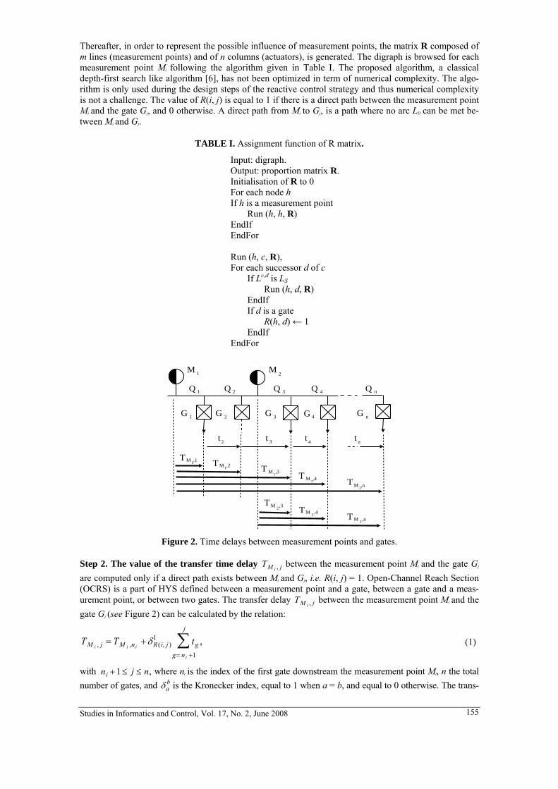
Thereafter, in order to represent the possible influence of measurement points, the matrix R composed of m lines (measurement points) and of n columns (actuators), is generated. The digraph is browsed for each measurement point Mi following the algorithm given in Table I. The proposed algorithm, a classical depth-first search like algorithm [6], has not been optimized in term of numerical complexity. The algo-rithm is only used during the design steps of the reactive control strategy and thus numerical complexity is not a challenge. The value of R(i, j) is equal to 1 if there is a direct path between the measurement point Mi and the gate Gj, and 0 otherwise. A direct path from Mi to Gj, is a path where no arc LD can be met be-tween Mi and Gj.
TABLE I. Assignment function of R matrix.
Input: digraph. Output: proportion matrix R. Initialisation of R to 0 For each node h If h is a measurement point Run (h, h, R) EndIf EndFor Run (h, c, R), For each successor d of c If Lc,d is LS Run (h, d, R) EndIf If d is a gate R(h, d) ← 1 EndIf EndFor
T M ,11
G G
M
G G
M
G
QQQQQ
t t t t
T
1 2
1 2 3 4 n
1 2 3 4 n
2 3 4 n
M ,21 T M ,3
1 T M ,41 T M ,n
1
T M ,32 T M ,4
2 T M ,n2
Figure 2. Time delays between measurement points and gates.
Step 2. The value of the transfer time delay T between the measurement point MM i , j i and the gate Gj
are computed only if a direct path exists between Mi and Gj, i.e. R(i, j) = 1. Open-Channel Reach Section (OCRS) is a part of HYS defined between a measurement point and a gate, between a gate and a meas-urement point, or between two gates. The transfer delay T between the measurement point MM i , j i and the gate Gj (see Figure 2) can be calculated by the relation:
TM i , j = TM i ,ni+ δR(i, j )
1 tgg= ni +1
j
∑ , (1)
with where nni +1 ≤ j ≤ n, i is the index of the first gate downstream the measurement point Mi, n the total number of gates, and is the Kronecker index, equal to 1 when a = b, and equal to 0 otherwise. The trans-δa
b
Studies in Informatics and Control, Vol. 17, No. 2, June 2008 155

fer delay tg associated to each OCRS is computed from the OCRS dynamics model described thereafter.
Usually, Saint Venant equations are used for the modelling of open channel dynamics. The analytic reso-lution of these two-coupled partial differential equations [5] is not possible. As discussed in [14, 1] dis-cretisation methods can be used to find a solution. Otherwise, a modelling method detailed in [16] based on the simplification and linearization of Saint Venant equations can be used. This method is based on the identification for each OCRS of a transfer function plus transfer delay (2) for a reference discharge Qe [8], according to the OCRS geometrical characteristics.
,1
)( 221 swsw
esFs
++=
−τ (2)
where the coefficients w1, w2 and the pure delay τ are computed according to the identified celerity and diffusion parameters Ce and De, and to the adimensional coefficient CL which is defined by:
CL =2Ce X9De
, (3)
where X is the OCRS length, Ce and De are expressed as:
Ce =1L2
∂J∂Qe
∂L∂x
−∂JL∂y
⎡
⎣ ⎢
⎤
⎦ ⎥ ,
De =1
L ∂J∂Qe
,
⎧
⎨
⎪ ⎪
⎩
⎪ ⎪
(4)
where L is the surface width, y the discharge depth, J the friction slope expressed with the Manning-
Strickler relation as J =Qe
2P43
K 2S103
, where K is the Strickler coefficient, P the wetted perimeter and S the
wetted surface.
As displayed in Table II, the order of the transfer function depends on the CL value. When CL ≤ 49 , the
OCRS is short and can be modelled by a first order transfer function without delay, when 49 < CL ≤ 1, a
delay is added to a first order transfer function and when CL > 1, the OCRS is long enough and can be modelled by a second order transfer function with delay.
TABLE II. Continuous transfer functions F(s) corresponding to CL.
221
194
194
1)(1
1)(1
11)(
)(
swswesFC
swesFC
swsFC
sFC
s
L
s
L
L
L
++=>
+=≤<
+=≤
−
−
τ
τ
The time delay tg (see relation (1)) depends on the network configuration (the followed path). It is com-puted from the step response of the transfer function, which is identified around the reference discharge Qe, and corresponds to the time so that 50% of the step response is reached. Then, the transfer delay T
(1) is expressed according to the sampling period TM i , j
s:
kdM i , j =TM i , j
Ts
⎢
⎣ ⎢
⎥
⎦ ⎥ +1, (5)
where x⎣ ⎦ denotes the integer part of x. The measured water quantity in Mi will arrive on gate Gj at the date:
ℑ M i , j = (k + kdM i , j )Ts. (6)
Studies in Informatics and Control, Vol. 17, No. 2, June 2008 156
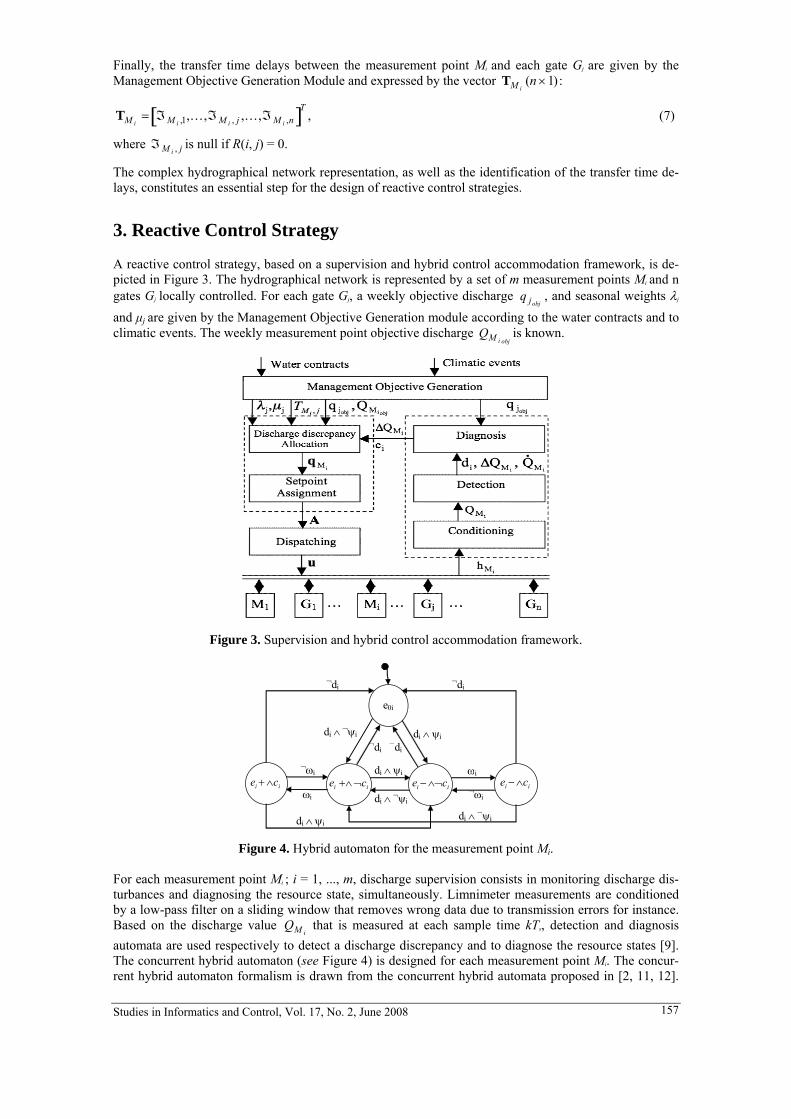
Finally, the transfer time delays between the measurement point Mi and each gate Gj are given by the Management Objective Generation Module and expressed by the vector TM i
(n ×1):
TM i
= ℑM i ,1,K,ℑM i , j ,K,ℑ M i ,n[ T,] (7)
where ℑ is null if R(i, j) = 0. M i , j
The complex hydrographical network representation, as well as the identification of the transfer time de-lays, constitutes an essential step for the design of reactive control strategies.
3. Reactive Control Strategy
A reactive control strategy, based on a supervision and hybrid control accommodation framework, is de-picted in Figure 3. The hydrographical network is represented by a set of m measurement points Mi and n gates Gj locally controlled. For each gate Gj, a weekly objective discharge , and seasonal weights λq jobj
j
and μj are given by the Management Objective Generation module according to the water contracts and to climatic events. The weekly measurement point objective discharge is known. QM i obj
Figure 3. Supervision and hybrid control accommodation framework.
e0i
ii ce ¬∧+ ii ce ∧¬− ii ce ∧− ii ce ∧+
di ∧ ¬ψi di ∧ ψi ¬di
¬di ¬di
¬ωi di ∧ ψi ωi
ωi di ∧ ¬ψi ¬ωi
di ∧ ¬ψi di ∧ ψi
¬di
Figure 4. Hybrid automaton for the measurement point Mi.
For each measurement point Mi ; i = 1, ..., m, discharge supervision consists in monitoring discharge dis-turbances and diagnosing the resource state, simultaneously. Limnimeter measurements are conditioned by a low-pass filter on a sliding window that removes wrong data due to transmission errors for instance. Based on the discharge value Q that is measured at each sample time kTM i s, detection and diagnosis automata are used respectively to detect a discharge discrepancy and to diagnose the resource states [9]. The concurrent hybrid automaton (see Figure 4) is designed for each measurement point Mi. The concur-rent hybrid automaton formalism is drawn from the concurrent hybrid automata proposed in [2, 11, 12].
Studies in Informatics and Control, Vol. 17, No. 2, June 2008 157
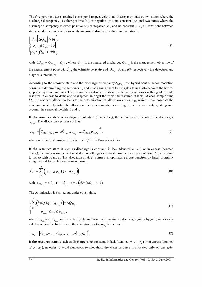
The five pertinent states retained correspond respectively to no-discrepancy state e0, two states where the discharge discrepancy is either positive (e+) or negative (e− ) and constant (ci), and two states where the discharge discrepancy is either positive (e+) or negative (e− ) and no constant ( ic¬ ). Transitions between states are defined as conditions on the measured discharge values and variations:
[ ][ ]
[ ]⎪⎩
⎪⎨
⎧
>
<Δ>Δ
,:,0:,:
iMi
Mi
iMi
dthQQ
thQd
i
i
i
&ωψ (8)
with where is the measured discharge, Q is the management objective of
the measurement point M
ΔQM i= QM i obj
− QM i, QM i M i obj
i, the estimate derivative of Q , thiMQ& M i i and dthi respectively the detection and
diagnosis thresholds.
According to the resource state and the discharge discrepancy ΔQM i, the hybrid control accommodation
consists in determining the setpoints qj, and in assigning them to the gates taking into account the hydro-graphical system dynamics. The resource allocation consists in recalculating setpoints with a goal to route resource in excess to dams and to dispatch amongst the users the resource in lack. At each sample time kTs, the resource allocation leads to the determination of allocation vector which is composed of the new computed setpoints. The allocation vector is computed according to the resource state e
qM i
i taking into account the seasonal weights λj and μj.
If the resource state is no diagnose situation (denoted E0), the setpoints are the objective discharges . The allocation vector is such as: q jobj
qM i
= δR(i,1)1 q1obj ,K,δR(i, j )
1 q j obj,K,δR(i,n )
1 qn obj[ T,] (9)
where n is the total number of gates, and is the Kronecker index. δab
If the resource state is such as discharge is constant, in lack (denoted e− ∧ ci) or in excess (denoted e+ ∧ ci), the water resource is allocated among the gates downstream the measurement point Mi, according to the weights λj and μj. The allocation strategy consists in optimizing a cost function by linear program-ming method for each measurement point:
fM i= δ R ( i, j )
1 χ M i , jq j − q jobj( )(
j=1
n
∑ ,) (10)
with χ M i , j= γ 1
λ j+ γ −1( ) 1
μ j,γ = 1
2 sign(ΔQM i) +1( ).
The optimization is carried out under constraints:
R(i, j)(q j − q jobj)( )= ΔQM i
,j=1
n
∑q jmin
≤ q j ≤ q jmax,
⎧
⎨ ⎪
⎩ ⎪
(11)
where and are respectively the minimum and maximum discharges given by gate, river or ca-nal characteristics. In this case, the allocation vector is such as:
q jminq jmax
qM i
qM i
= δR(i,1)1 q1,K,δR(i, j )
1 q j ,K,δR(i,n )1 qn[ T
,] (12)
If the resource state is such as discharge is no constant, in lack (denoted ) or in excess (denoted
), in order to avoid numerous re-allocation, the water resource is allocated only on one gate, ice ¬∧−
ice ¬∧+
Studies in Informatics and Control, Vol. 17, No. 2, June 2008 158
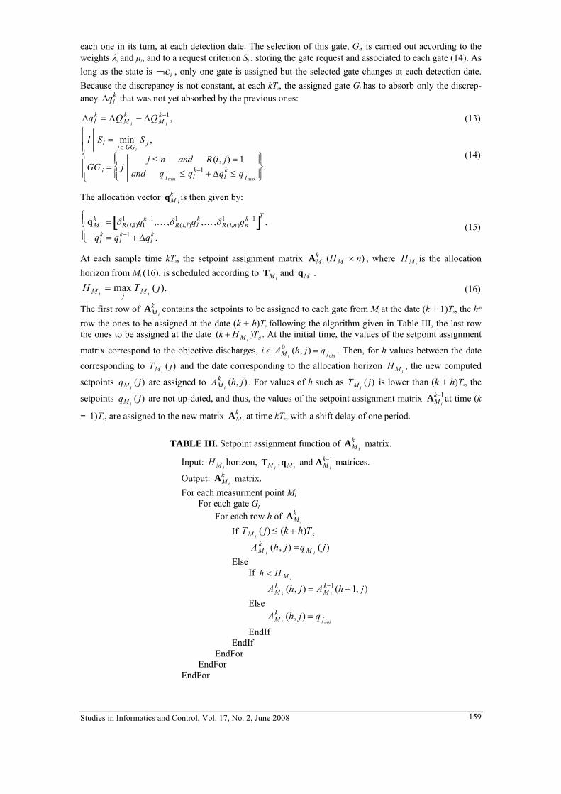
each one in its turn, at each detection date. The selection of this gate, Gl, is carried out according to the weights λj and μj, and to a request criterion Sj , storing the gate request and associated to each gate (14). As long as the state is , only one gate is assigned but the selected gate changes at each detection date. Because the discrepancy is not constant, at each kT
ic¬s, the assigned gate Gl has to absorb only the discrep-
ancy that was not yet absorbed by the previous ones: Δqlk
Δqlk = ΔQM i
k − ΔQM i
k−1, (13)
l Sl = minj ∈GGi
S j ,
GG i = jj ≤ n and R (i, j) = 1
and q jmin≤ ql
k−1 + Δqlk ≤ q jmax
⎧ ⎨ ⎪
⎩ ⎪
⎫ ⎬ ⎪
⎭ ⎪ .
⎧
⎨ ⎪ ⎪
⎩ ⎪ ⎪
(14)
The allocation vector is then given by: qMk
i
qM i
k = δ R (i,1)1 q1
k−1,K ,δ R(i,l )1 ql
k ,K ,δ R (i,n )1 qn
k−1[ T,
qlk = ql
k−1 + Δqlk .
]⎧ ⎨ ⎪
⎩ ⎪ (15)
At each sample time kTs, the setpoint assignment matrix , where is the allocation horizon from M
AM i
k (HM i× n) H M i
i (16), is scheduled according to and . TM iqM i
H M i= max
jTM i
( j). (16)
The first row of contains the setpoints to be assigned to each gate from MAM i
ki at the date (k + 1)Ts, the hth
row the ones to be assigned at the date (k + h)Ts following the algorithm given in Table III, the last row the ones to be assigned at the date . At the initial time, the values of the setpoint assignment
matrix correspond to the objective discharges, i.e. . Then, for h values between the date corresponding to T and the date corresponding to the allocation horizon , the new computed
setpoints are assigned to . For values of h such as T is lower than (k + h)T
(k + HM i)Ts
AM i
0 (h, j) = q jobj
M i( j) H M i
qM i( j) AM i
k (h, j) M i( j) s, the
setpoints are not up-dated, and thus, the values of the setpoint assignment matrix at time (k
− 1)T
qM i( j) AM i
k−1
s, are assigned to the new matrix at time kTAM i
ks, with a shift delay of one period.
TABLE III. Setpoint assignment function of matrix. AM i
k
Input: horizon, H M iTM i
,qM iand AM i
k−1 matrices.
Output: matrix. AM i
k
For each measurment point Mi For each gate Gj
For each row h of AM i
k
If TM i( j) ≤ (k + h)Ts
AM i
k (h , j) =q M i( j)
Else If h < H M i
AM i
k (h, j) = AM i
k−1(h + 1, j) Else AM i
k (h, j) = q jobj
EndIf EndIf EndFor EndFor EndFor
Studies in Informatics and Control, Vol. 17, No. 2, June 2008 159
TABLE IV. Assignment function of α M i matrix.
Input: digraph. Output: α matrix. M i
Initialisation of the diagonal of α M i to 0,
g ← first gate successor of Mi Run (Mi, g, ) α M i
Run (Mi, g, ), α M i
For each successor d of c If Lc,d is LS and d is a gate Run (Mi, g, α M i
) αM i
(d ,d) ← 1 EndIf EndFor
Finally, the setpoints are dispatched with the control period Tc = κTs, where k is an integer. The control
setpoint vector denoted u (1 × n) is updated at each date ′ k Tc , where ′ k = kκ , thanks to the assignment
matrix and the α diagonal control accommodation matrix, with AM i
kM i
(n × n) H = 1κ max
1≤ i≤m(H M i
) the
control horizon. For each measurement point Mi, the α M i matrix, the role of which is to capture the actual
influence of the measurement point on the gates, must be determined. In order to generate the ma-trix, the weighted digraph (see Figure 1.c and d) is browsed using the algorithm given in table IV, for each measurement point M
α M i
i. The control setpoint vector u ′ k ′ (1 × n) is calculated by:
u ′ k ( j) = αM i( j, j)AM i
′ k
i=1
m
∑ (1, j). (17)
The setpoint dispatching leads to the application of the most recently calculated setpoints. This method increases the control strategy reactivity, because discharge variations between two control dates are taken into account.
4. Management of a Networked Dam-River System
The problem addressed in this section deals with the water asset management of the Purple Dam-River System (PDRS) which is a part of a real networked hydrographical system. The PDRS is characterized by a gridded network configuration with two diffluences and one confluence. The PDRS is composed of the Purple channel upstream reach which supplies the Pink river, the Blue and the Orange channels, the Yel-low, Jade and Cyan rivers. The Blue channel supplies the Green, the Red and the Magenta channels and the Indigo river. The Orange channel supplies the Black and the Magenta channels and the Indigo river (see Figure 5). The Red channel and Magenta channel supply downstream dams. The channels are com-posed of several reach sections, i.e. a part between two measurement points, about thirty kilometres length. It is considered that all the OCRS of the reach sections have trapezoidal profiles.
Studies in Informatics and Control, Vol. 17, No. 2, June 2008 160
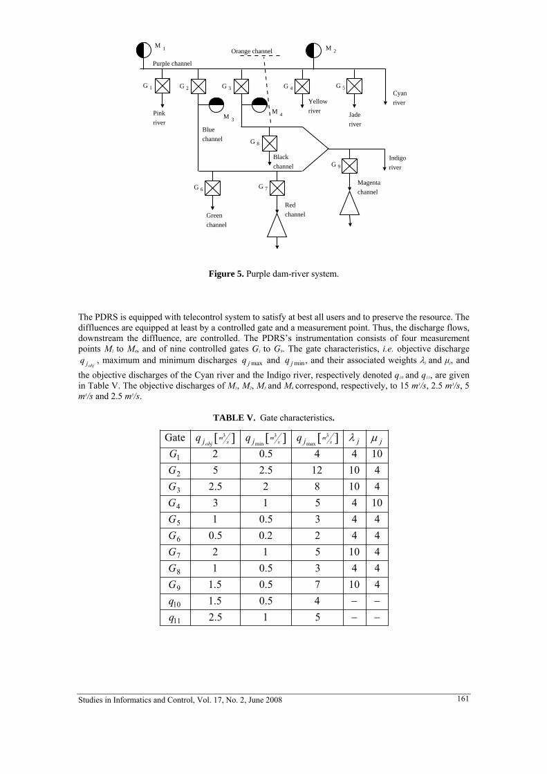
M
G
Purple channel
Pink
riverBlue
channel
Green
channel
Red
channel
Magenta
channel
Indigo
river
Yellow
riverJade
river
Cyan
river
Black
channel
Orange channel1 M 2
1 G 2 G 3 G 4 G 5
G 6
G 8
G 7
G 9
M 3
M 4
Figure 5. Purple dam-river system.
The PDRS is equipped with telecontrol system to satisfy at best all users and to preserve the resource. The diffluences are equipped at least by a controlled gate and a measurement point. Thus, the discharge flows, downstream the diffluence, are controlled. The PDRS’s instrumentation consists of four measurement points M1 to M4, and of nine controlled gates G1 to G9. The gate characteristics, i.e. objective discharge
, maximum and minimum discharges and , and their associated weights λq jobjq j max q j min j and μj, and
the objective discharges of the Cyan river and the Indigo river, respectively denoted q10 and q11, are given in Table V. The objective discharges of M1, M2, M3 and M4 correspond, respectively, to 15 m3/s, 2.5 m3/s, 5 m3/s and 2.5 m3/s.
TABLE V. Gate characteristics.
Gate q jobjm3
s[ ] q jminm3
s[ ] q jmaxm3
s[ ] λ j μ j
G1 2 0.5 4 4G2 5 2.5 12 10 4G3 2.5 2 8 10 4G4 3 1 5 4G5 1 0.5 3 4G6 0.5 0.2 2 4 4G7 2 1 5 10G8 1 0.5 3 4G9 1.5 0.5 7 10 4q10 1.5 0.5 4 − −q11 2.5 1 5 − −
10
104
44
Studies in Informatics and Control, Vol. 17, No. 2, June 2008 161

(a)
(b)
M
1 2 3 4 5
6
7 8
9 10
11
1 M2
M 3
M 4
G 1 G 2G 3 G 4 G 5
G 6 G 7
G 8
G 9
M 1 M 2G 1 G 2 G 3 G 4 G 5
M 3
M 4
G 6 G 7
G 8
G 9
Figure 6. (a) PDRS representation, (b) its associated digraph representation.
The PDRS is subjected to disturbances upstream the Purple Channel. The considered management sce-nario consists in:
- Allocating the water quantities in lack, due to withdrawals, amongst the Pink and the Yellow rivers,
- Allocating the water quantities in excess, due to water restitution, toward the Red channel and Magenta channel which supply dams.
Thus, the weights λj that are associated to the gates G2, G3, G7 and G9 are the maximum ones (see Table V). In addition, the maximum weights μj are associated to the gates G1 and G4 that correspond to minor priority uses.
The first step of the proposed method is based on the digraph representation of the PDRS, shown in Fig-ure 6, which leads to the determination of the R and α M i
matrices according to the algorithms given in Tables I and IV, respectively. The matrix R is given by relation (18). The values of R(1, j), i.e. from the measurement point M1 to the gates, is equal to 1 for the gates G1 to G5 because there is a direct path be-tween this measurement point and these gates, and 0 otherwise.
R =
1 1 1 1 1 0 0 0 00 0 0 0 1 0 0 0 00 0 0 0 0 1 1 0 10 0 0 0 0 0 0 1 1
⎡
⎣
⎢ ⎢ ⎢ ⎢
⎤
⎦
⎥ ⎥ ⎥ ⎥
. (18)
The diagonal matrices α M 1to are given by (19). The fifth value of α M 4
α M 1is equal to 0 because meas-
urement point M2 is located upstream gates G5.
α M 1= diag 1, 1, 1, 1, 0, 0, 0, 0, 0{ },
α M 2= diag 0, 0, 0, 0, 1, 0, 0, 0, 0{ },
α M 3= diag 0, 0, 0, 0, 0, 1, 1, 0, 1{ ,
α M 4= diag 0, 0, 0, 0, 0, 0, 0, 1, 1{ }.
} (19)
Studies in Informatics and Control, Vol. 17, No. 2, June 2008 162

1
B
X
y
I
f
Figure 7. Geometrical characteristics of a trapezoidal profile.
The second step aims at determining the transfer time delays T . The HYS have been modelled ac-cording to the specific length and profile section of each OCRS. The OCRS are numbered from 1 to 11 (see Figure 6.a). The OCRS with trapezoidal profile is characterized by the bottom width B, the average fruit of the banks f, the profile length X, the discharge depth y and the slope I (see Figure 7). The geomet-rical characteristics of the OCRS are given in Table VI.
M i , j
For trapezoidal profiles, the celerity and diffusion parameters Ce and De are expressed as:
Ce =Qe
L2 − f +L3
2BPy
+5LS
−2y
⎛
⎝ ⎜ ⎜
⎞
⎠ ⎟ ⎟
⎡
⎣ ⎢ ⎢
⎤
⎦ ⎥ ⎥
De =Qe2LJ
.
⎧
⎨ ⎪ ⎪
⎩ ⎪ ⎪
, (20)
with L = B + 2fy, S = yB + fy2, P = B + 2y 1+ f 2 , and the slope J is equivalent to the reach slope I for a non critical discharge.
In the studied case, the transfer function is estimated for one operating point for each OCRS. Parameters of the transfer functions identified for reference discharges Qe, are given in Table VII. The response times t are computed from the step response of every identified model, as the time such that 50% of the step response is reached. Then, the transfer delays tg are computed according to response times t and to the PDRS configuration (see Figure 8). The measurement points M2, M3 and M4, are located close to their re-spective upstream gates G4, G2 and G3.
TABLE VI. Geometrical characteristics of the OCRS.
OCRS B m[ ] f X m[ ] I K1 5.4 0.8 1200 5.10−4 702 5.4 0.95 3700 5.10−4 703 5.2 0.95 1500 5.10−4 704 5 0.9 2400 5.10−4 705 4.8 0.9 1200 5.10−4 706 4 0.95 11000 2.10−4 707 4 0.95 15000 2.10−4 708 4 0.95 2625 4.10−4 709 3 0.95 10000 4.10−4 70
10 3 0.95 5000 3.10−4 7011 3 0.95 2000 2.10−4 70
Studies in Informatics and Control, Vol. 17, No. 2, June 2008 163

TABLE VII. Parameters of the transfer functions.
[ ] [ ] [ ]
136000196741146601650314900036105.11077103970531200043145.29180054044320016195.28
1240045402182000093975.47859025901098000074255670724006735.25
11804198580010575.5460769077883
14806240124613239500570151
OCRS 213
sssm twwQe τ
Finally, the transfer time delays between the measurement points Mi and each gate Gj are expressed ac-cording to the sample time Ts (equal to 120 s) using equation (5). The vectors are given by equation (21). Then, at each sample time kT
kdM i
s, the vectors are computed using (6). TM i
kd M 1= 4, 16 , 21, 31, 37, 0, 0, 0, 0[ ]T ,
kd M 2= 0, 0, 0, 0, 6, 0, 0, 0, 0[ T ,
kd M 3= 0, 0, 0, 0, 0, 72 , 175, 0, 201[ ]T ,
kd M 4= 0, 0, 0, 0, 0, 0, 0, 65, 115[ ]T .
] (21)
2 3 4 5
7 8 11
(a)
(b)
(c)
1
6
9 10 11
M 1 M 2
G 1 G 2G 3 G 4 G 5
M 3
G 6 G 7 G 9
G 9G 8
M 4
T M ,11 T M ,2
1 T M ,31 T M ,4
1 T M ,51
T M ,52
t t t2 3 4
t5
t7
t9
T M ,63 T M ,7
3 T M ,93
t9
T M ,84
T M ,94
Figure 8. Time delays between measurement points and gates for (a) Purple channel stream, (b) Blue
channel stream, and (c) Orange channel stream.
Studies in Informatics and Control, Vol. 17, No. 2, June 2008 164

The hydrographical system is subjected to disturbances upstream the measurement points M1 (see Figure 9.a). Figure 9 shows discharges measured on M1, M3 and M4, and the discharges q10 and q11 in the case where no reactive strategy is used (dotted line) and where the reactive strategy is used (continuous line). The results on M2 and the setpoints dispatched on gates G5 are not detailed herein.
For each canal reach, Figures 10, 11 and 12 show measured discharges in (a), the corresponding resource states diagnosis in (b), and the new setpoints that have been dispatched at the gates. As an example, the discharge measured on M1 is depicted in Figure 10.a, the corresponding diagnosed resource state in Figure 10.b, the setpoints dispatched on gates G1, G2, G3 and G4 respectively, in Figures 10.c, 10.d, 10.e, and 10.f, and the resource at the end of the channel G10 in Figure 10.g. The setpoint dispatched on gate G9 is result-ing from the addition of the new setpoints calculated from M3 and M4 (see Figures 11.e and 12.d). Thus, in Figure 11.e, and in Figure 12.d, the setpoint allocated starting from M3 and, respectively, from M4 are rep-resented in dashed line, and the resulting setpoint dispatched on gate G9 in continuous line.
14.5
15
15.5
(a)
QM
1 [m
3 /s]
5
5.2
5.4
(b)
QM
3 [m
3 /s]
2.6
2.8
(c)
QM
4 [m
3 /s]
1
1.5
2
(d)
q 10 [m3 /s
]
0 2 4 6 8 10 12 14 16 18 20 22 24 26 28 30 32 34 36 382.4
2.5
2.6
(e)
q 11 [
m3 /s
]
Time [h] Figure 9. Discharges (a) Q , (b) , (c) Q , (d) qM 1
QM 3 M 4 10, (e) q11, with control accommodation (continu-ous line) and without (dotted line).
14.515
15.5
(a)
QM
1 [m3 /s
]
E− CE− nC
E0E+ nCE+ C
(b)
Sta
te
1.8
2
(c)
q 1 [m3 /s
]
5
5.2
5.4
(d)
q 2 [m3 /s
]
2.6
2.8
(e)
q 3 [m3 /s
]
2.6
2.8
3
)
q 4 [m3 /s
]
0 2 4 6 8 10 12 14 16 18 20 22 24 26 28 30 32 34 36 381.4
1.5
1.6
(g)
q 10 [m3 /s
]
Time [h] Figure 10. (a) Discharge Q , (b) diagnosed states from MM 1 1. Setpoints assigned to (c) gate G1, (d) gate
G2, (e) gate G3, (f) gate G4, and (g) gate G10.
When no strategy is applied, the water quantities in lack or in excess are not allocated on the gates G1 to G5 (see dotted line in Figure 10.c, d, e and f), as shown by the values of the measured discharges on M3
and M4 (see dotted line in Figure 9.b and c). The volumes of water due to the disturbances are propagated upstream to downstream on the Purple channel, and the discharge at the end of the channel q10 is far from its discharge objective from the 6q10 obj
th hour to the 20th hour (see dotted line in Figure 9.d).
When the reactive strategy is applied, as defined by the management scenario, the water quantities in lack are allocated amongst the gates G1 and G4 (see Figure 10.c and f), and the water quantities in excess are allocated amongst the gates G2 and G3 (see Figure 10.d and e) and finally amongst the gates G7 and G9 (see
Studies in Informatics and Control, Vol. 17, No. 2, June 2008 165
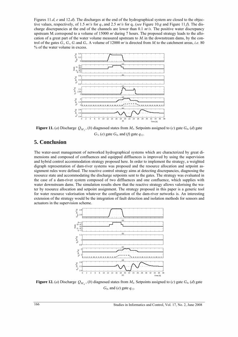
Figures 11.d, e and 12.d). The discharges at the end of the hydrographical system are closed to the objec-tive values, respectively, of 1.5 m3/s for q10 and 2.5 m3/s for q11 (see Figure 10.g and Figure 11.f). The dis-charge discrepancies at the end of the channels are lower than 0.1 m3/s. The positive water discrepancy upstream M1 correspond to a volume of 15000 m3 during 7 hours. The proposed strategy leads to the allo-cation of a great part of the water volume measured upstream to M1 in the downstream dams, by the con-trol of the gates G2, G3, G7 and G9. A volume of 12000 m3 is directed from M1 to the catchment areas, i.e. 80 % of the water volume in excess.
5
5.2
5.4
(a)
QM
3 [m3 /s
]
E− CE− nC
E0E+ nC
E+
(b)S
tate
0.4
0.5
0.6
(c)
q 6 [m3 /s
]
22.05
2.1
(d)
q 7 [m3 /s
]
1
1.5
2
(e)
q 9 [m3 /s
]
0 2 4 6 8 10 12 14 16 18 20 22 24 26 28 30 32 34 36 382.4
2.5
2.6
(f)
q 11 [m
3 /s]
Time [h] Figure 11. (a) Discharge Q , (b) diagnosed states from MM 3 3. Setpoints assigned to (c) gate G6, (d) gate
G7, (e) gate G9, and (f) gate q11.
5. Conclusion
The water-asset management of networked hydrographical systems which are characterized by great di-mensions and composed of confluences and equipped diffluences is improved by using the supervision and hybrid control accommodation strategy proposed here. In order to implement the strategy, a weighted digraph representation of dam-river systems was proposed and the resource allocation and setpoint as-signment rules were defined. The reactive control strategy aims at detecting discrepancies, diagnosing the resource state and accommodating the discharge setpoints sent to the gates. The strategy was evaluated in the case of a dam-river system composed of two diffluences and one confluence, which supplies with water downstream dams. The simulation results show that the reactive strategy allows valorising the wa-ter by resource allocation and setpoint assignment. The strategy proposed in this paper is a generic tool for water resource valorisation whatever the configuration of the dam-river networks is. An interesting extension of the strategy would be the integration of fault detection and isolation methods for sensors and actuators in the supervision scheme.
2.6
2.8
(a)
QM
4 [m3 /s
]
E− CE− nC
E0E+ nCE+ C
(b)
Sta
te
0.9
1
1.1
(c)
q 8 [m3 /s
]
1
2
(d)
q 9 [m3 /s
]
0 2 4 6 8 10 12 14 16 18 20 22 24 26 28 30 32 34 36 382.4
2.5
2.6
(e)
q 11 [m
3 /s]
Time [h] Figure 12. (a) Discharge , (b) diagnosed states from MQM 4 4. Setpoints assigned to (c) gate G8, (d) gate
G9, and (e) gate q11.
Studies in Informatics and Control, Vol. 17, No. 2, June 2008 166
REFERENCES
1. ABBOTT, M. and D. BASCO, Computational Fluid Dynamics: An Introduction for Engineers, Longman scientific and technical; New York, John Wiley and Son, 1989.
2. BLACKMORE, L., S. FUNIAK, and B. C. WILLIAMS, A Combinad Stochastic and Greedy Hy-brid Estimation Capability for Concurrent Hybrid Models with Autonomous Mode Transitions, Robotics and Autonomous Systems, Vol. 56, 2008, pp. 105–129.
3. CEMBRANO, G., G. WELLS, J. QUEVEDO, R. PEREZ, and R. ARGELAGUET, Optial Control of a Water Distribution Network in a Supervisory Control System, Control Engineering Practice, vol. 8, 2000, pp. 1177–1188.
4. CHAN, C., W. KRITPIPHAT, and P. TONTIWACHWUTHIKUL, Development of an Intelligent Control System for a Municipal Water Distribution Network, IEEE Canadian conference on Elec-trical and Computer Engineering, Vol. 2, 1999, pp. 1108–1113.
5. CHOW, V. T., D. R. MAIDMENT, and L. W. MAYS, Applied Hydrology, New York, Paris, McGraw-Hill, 1988.
6. CORMEN, T. H., C. E. LEISERSON, R. L. RIVEST, and C. STEIN, Introduction to Algorithms, Second Edition, MIT Press, 2001.
7. DUVIELLA, E., P. CHIRON, and P. CHARBONNAUD, Hybrid Control Accommodation for Wa-ter-asset Management of Hydraulic Systems Subjected to Large Operating Conditions, ALSIS06, 1st IFAC Workshop on Applications of Large Scale Industrial Systems, Helsinki, Finland, August 30-31, 2006.
8. DUVIELLA, E., P. CHIRON, and P. CHARBONNAUD, Multimodelling Steps for Free-surface Hydraulic Systems Control, ICINCO 2006, 3rd International Conference on Informatics in Control, Automation and Robotics, Signal Processing, Systems Modelling and Control, Setubal, Portugal, 1-5 August., 2006.
9. DUVIELLA, E., P. CHIRON, P. CHARBONNAUD, and P. HURAND, Supervision and Hybrid Control Accommodation for Water Asset Management, Control Engineering Practice (CEP), Vol. 15, pp. 17–27, 2007.
10. FAYE,R. M., S. SAWADOGO, A. NIANG, and F. MORA-CAMINO, An Intelligent Decision Sup-port System for Irrigation System Management, IEEE International Conference on Systems, Man and Cybernetics, SMC’98, October 11-14, San Diego, USA, Vol. 4, 1998, pp. 3908–3913.
11. FUNIAK, S., L. J. BLACKMORE, and B. C. WILLIAMS, Gaussian Particle Filtering for Concur-rent Hybrid Models with Autonomous Transitions, submitted to Journal of Artificial Intelligence Research, 2004.
12. HOFBAUR, M. W. and B. C. WILLIAMS, Hybrid Diagnosis with Unknown Behaviorla Modes, International Workshop on Principles of Diagnosis (Dx-02), Semmering, Austria, May 2-4, pp. 97–105, 2002.
13. ISLAM, A., N. S. RAGHUWANSHI, R. SINGH, and D. J. SEN, Comparison of Gradually Varied Flow Computation Algorithms for Open-channel Network, Journal of irrigation and drainage en-gineering, Vol. 131, No. 5, 2005, pp. 457–465.
14. KUTIJA, V. and C.-J.-M. HEWETT, Modelling of Supercritical Flow Conditions Revisited; NewC scheme, Journal of hydraulic research, Vol. 40, No. 2, 2002, pp. 145–152.
Studies in Informatics and Control, Vol. 17, No. 2, June 2008 167

15. LISOUNKIN, A., A. SABOV, and G. SCHRECK, Interpreter Based Model Check for Distribu-tion Networks, IEEE international conference on industrial informatics, INDIN’O4, 24-26 juin, 2004, pp. 431–435.
16. LITRICO, X. and D. GEORGES, Robust Continuous-time and Discrete-time Flow Control of a Dam-river System. (i) modeling, Applied Mathematical Modelling 23, 1999, pp. 809–827.
17. MANSOUR, H. E. F., D. GEORGES, and G. BORNARD, Optimal Control of Complex Irrigation Systems via Decomposition-Coordination and the Use of Augmented Lagrangian, IEEE, Interna-tional Conference on Control Applications, Trieste, Italy, 1998, pp. 3874–3879.
18. NAIDU, B. J., S. M. BHALLAMUDI, and S. NARASIMHAN, GVF Computation in Tree-type Channel Networks, Journal of hydraulic engineering, Vol. 123, No. 8, 1997, pp. 700–708.
Studies in Informatics and Control, Vol. 17, No. 2, June 2008 168
Studies in Informatics and Control, Vol. 17, No. 2, June 2008 169
Presentation of Some Metaheuristics for the Optimization of Complex Systems
Fatma Tangour1, 2 and Pierre Borne1
1LARA, École Nationale d'Ingénieurs de Tunis, BP 37, Le Belvédère 1002 Tunis, Tunisie 2LAGIS, École Centrale de Lille, Cité scientifique, BP 48, 59651 Villeneuve d'Ascq Cedex, France
[email protected], [email protected]
Abstract: Some metaheuristics for the optimization of complex systems are proposed in this paper. The metaheuristic approaches can be separate in two classes: the local search techniques and the global ones. An important difficulty which appears in complex optimization problems is the existence of constraints which can be strict and inviolable or soft. To resolve these problems, some hybrid approaches are considered.
Keywords: Optimization, complex systems, metaheuristics, tabu search, simulated annealing, genetic algorithms, ant colony optimization, particle swarm optimization, tunneling Algorithms.
Fatma Tangour graduated from Ecole Normale Superieure de l’Enseignement Technique of Tunis, received the Master degree of automatic and signal treatment in 2004 and Doctoral degree from the Ecole Nationale d’Ingénieur de Tunis and the Ecole Centrale de Lille in 2007. She is currently researcher in LARA Automatique at the Ecole Nationale d’Ingénieur de Tunis and working with the higher institute of sciences applied and technology of Kairouan, Tunisia. Her research interests are in the area of optimization methods for discrete events systems, computer science and operational research.
Pierre Borne received the Master degree of Physics in 1967, the Masters of Electronics, of Mechanics and of Applied Mathematics in 1968. The same year he obtained the Diploma of "Ingénieur IDN" (French "Grande Ecole"). He obtained the PhD in Automatic Control of the University of Lille in 1970 and the DSc of the same University in 1976. He became Doctor Honoris Causa of the Moscow Institute of Electronics and Mathematics (Russia) in 1999, of the University of Waterloo (Canada) in 2006 and of the Polytechnic University of Bucarest (Romania). He is author or co-author of about 200 Journal articles and book chapters, and of 34 plenary lectures and of more than 250 communications in international conferences. He has been the supervisor of 68 PhD thesis and is author of 20 books. He is Fellow of IEEE and has been President of the IEEE/SMC society in 2000 and 2001. He is presently Professor “de classe exceptionnelle” at the Ecole Centrale de Lille and director of the french pluriformations national group of research in Automatic Control
1. Introduction
Many optimization problems such as combinatorial optimization [3, 31] ones are usually N-P hard problems which prevent the implementation of exact used solving methodologies. It is the reason why engineers prefer to use metaheuristics which are able to produce good solutions in a reasonable computation time. The metaheuristic approaches can be separate in two classes: the local search techniques and the global ones. Among the local search techniques the Tabu search [14] is the more known. The other methods usually involve a part of stochastic approach, like the Simulated Annealing [1, 6, 27], the Genetic or Evolutionary Algorithms [28, 29, 36], the Ant Colony Optimization [11] or the Particle Swarm Optimisation [4, 8].An important difficulty which appears in complex optimization problems is the existence of constraints which can be strict and inviolable or soft but with penalization which increase strongly with the degree of violation.
A possible acceleration of the convergence can be obtained by using tunnelling algorithms.
The muliobjective optimization is considered at the end of this paper with presentation of the OWA approach, of the Choquet integral and the Pareto optimality.
2. Tabu Search
Tabu search [12, 15, 16] is a local optimization method which enhances the performance of a local search method by using memory of the previous obtained solutions in order to permit to escape to a local optimum. It is an iterative local search procedure which enables to move from a solution to another solution in its neighbourhood until stopping criterion is satisfied. In practice the main Tabu search approach consists to determine, starting from a solution, the best solution in its immediate neighbourhood with interdiction to go to one of the N previous obtained solutions. Let us denote N(x) the list of the N solutions that have been visited in the recent past, at each step of iteration we eliminate the oldest solution of the list and we add the new on. With this method we avoid to have a cyclic evolution. It can appear that during some time we can have a degradation of the solution but it enables us to get out of a local optimum and to enlarge the search space.

Studies in Informatics and Control, Vol. 17, No. 2, June 2008 170
Another type of Tabu search corresponds to another definition of the Tabu list: which can prohibit solutions that have certain attributes or which can prevent certain solutions that contain prohibited attributes.
An example of Tabu search corresponds to the research of the smallest value in the following Notice Board.
The initial solution corresponds to a fitness equal to 12 and the Tabu list comports 5 elements, figure 1.
Figure 1. The research of smallest value
3. Simulated Annealing
3.1 Principle Simulated annealing [23, 32] is a generic probabilistic algorithm developed to solve global optimization problems for a function defined in a large search space. The simulated annealing has obtained excellent results in various complex problems known for their important combinatory properties. It is inspired of the physical thermic annealing. At each step of calculation of this algorithm the current solution is replaced by a nearly one chosen with a probability that depends of the variation of a fitness function (called the energy function by analogy with the physical process) via a parameter T (called the temperature) which gradually and regularly decrease during the process. In this approach the solution changes almost randomly for the large value of T and tends globally to obtain the minimum of the energy function as T tends to zero. The random evolution enables motions in which the energy can sometime increase which avoid falling and being trapped in a local minimum which can appear with usual downhill methods as the gradient method.
This algorithm can be presented as follows: let us denote s, T and e respectively the current state, temperature and energy, and sn and en respectively the new state and energy.
The process is initialize with s: = so and e: = eo which correspond to the initial state so of energy eo at time k = 0.
While the stopping condition is not satisfied (time k < km, and energy e>em), pick some state in the neighbourhood and compute its energy.
3.2 Example of simulated annealing algorithm
Initialization:
0 0( ), , 0,e E ss s k T T== = =
while mk k< and me e>
1ks + = neighbour ( )ks
( )1 1 1,k k k k ke E s e e e+ + += Δ = −
if random [ ] ( )0,1 exp /k ke T< −Δ
then 1 1 1: , : , : , 1k k k k k ks s e e T T k k+ + += = = = + return while
12 13 10 7 8 5 9 6 7 10 3 4 3
11 16 14 17 16 18 16 14 13 8 5 2 7
8 13 12 13 10 12 17 16 13 6 3 6 8
7 17 13 11 10 16 13 16 14 13 8 9 7
9 6 16 14 6 18 16 15 13 11 7 10 9
13 11 14 13 16 12 14 16 14 15 14 17 10
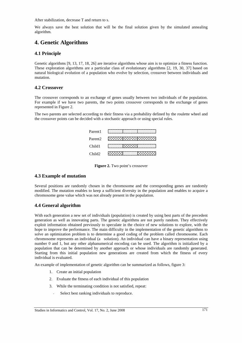
Studies in Informatics and Control, Vol. 17, No. 2, June 2008 171
After stabilization, decrease T and return to s.
We always save the best solution that will be the final solution given by the simulated annealing algorithm.
4. Genetic Algorithms
4.1 Principle
Genetic algorithms [9, 13, 17, 18, 26] are iterative algorithms whose aim is to optimize a fitness function. These exploration algorithms are a particular class of evolutionary algorithms [2, 19, 30, 37] based on natural biological evolution of a population who evolve by selection, crossover between individuals and mutation.
4.2 Crossover
The crossover corresponds to an exchange of genes usually between two individuals of the population. For example if we have two parents, the two points crossover corresponds to the exchange of genes represented in Figure 2.
The two parents are selected according to their fitness via a probability defined by the roulette wheel and the crossover points can be decided with a stochastic approach or using special rules.
Figure 2. Two point’s crossover
4.3 Example of mutation
Several positions are randomly chosen in the chromosome and the corresponding genes are randomly modified. The mutation enables to keep a sufficient diversity in the population and enables to acquire a chromosome gene value which was not already present in the population.
4.4 General algorithm
With each generation a new set of individuals (population) is created by using best parts of the precedent generation as well as innovating parts. The genetic algorithms are not purely random. They effectively exploit information obtained previously to speculate in the choice of new solutions to explore, with the hope to improve the performance. The main difficulty in the implementation of the genetic algorithms to solve an optimization problem is to determine a good coding of the problem called chromosome. Each chromosome represents an individual (a solution). An individual can have a binary representation using number 0 and 1, but any other alphanumerical encoding can be used. The algorithm is initialized by a population that can be determined by another approach or whose individuals are randomly generated. Starting from this initial population new generations are created from which the fitness of every individual is evaluated.
An example of implementation of genetic algorithm can be summarized as follows, figure 3:
1. Create an initial population
2. Evaluate the fitness of each individual of this population
3. While the terminating condition is not satisfied, repeat:
- Select best ranking individuals to reproduce.
Parent1
Parent2
Child2
Child1
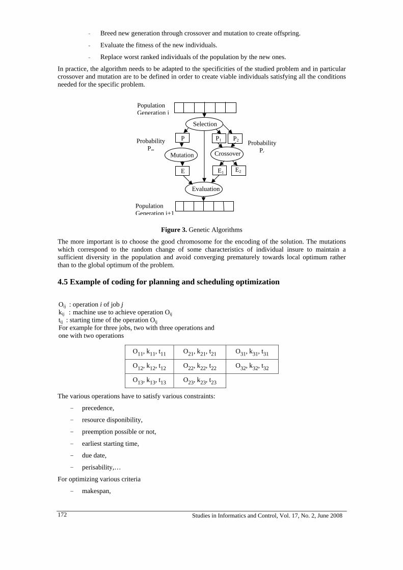
Studies in Informatics and Control, Vol. 17, No. 2, June 2008 172
- Breed new generation through crossover and mutation to create offspring.
- Evaluate the fitness of the new individuals.
- Replace worst ranked individuals of the population by the new ones.
In practice, the algorithm needs to be adapted to the specificities of the studied problem and in particular crossover and mutation are to be defined in order to create viable individuals satisfying all the conditions needed for the specific problem.
Figure 3. Genetic Algorithms
The more important is to choose the good chromosome for the encoding of the solution. The mutations which correspond to the random change of some characteristics of individual insure to maintain a sufficient diversity in the population and avoid converging prematurely towards local optimum rather than to the global optimum of the problem.
4.5 Example of coding for planning and scheduling optimization
O11, k11, t11 O21, k21, t21 O31, k31, t31
O12, k12, t12 O22, k22, t22 O32, k32, t32
O13, k13, t13 O23, k23, t23
The various operations have to satisfy various constraints:
- precedence,
- resource disponibility,
- preemption possible or not,
- earliest starting time,
- due date,
- perisability,…
For optimizing various criteria
- makespan,
Mutation
Population Generation i
Probability Pm
Selection
Evaluation
Crossover
P2 P1
P
E1 E2 E
ProbabilityPc
Population Generation i+1
Oij : operation i of job j kij : machine use to achieve operation Oij tij : starting time of the operation Oij For example for three jobs, two with three operations and one with two operations
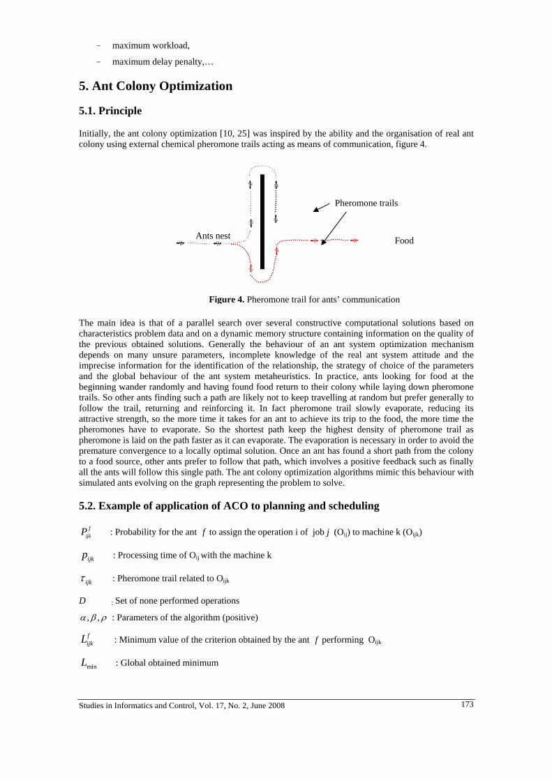
Studies in Informatics and Control, Vol. 17, No. 2, June 2008 173
- maximum workload,
- maximum delay penalty,…
5. Ant Colony Optimization
5.1. Principle
Initially, the ant colony optimization [10, 25] was inspired by the ability and the organisation of real ant colony using external chemical pheromone trails acting as means of communication, figure 4.
The main idea is that of a parallel search over several constructive computational solutions based on characteristics problem data and on a dynamic memory structure containing information on the quality of the previous obtained solutions. Generally the behaviour of an ant system optimization mechanism depends on many unsure parameters, incomplete knowledge of the real ant system attitude and the imprecise information for the identification of the relationship, the strategy of choice of the parameters and the global behaviour of the ant system metaheuristics. In practice, ants looking for food at the beginning wander randomly and having found food return to their colony while laying down pheromone trails. So other ants finding such a path are likely not to keep travelling at random but prefer generally to follow the trail, returning and reinforcing it. In fact pheromone trail slowly evaporate, reducing its attractive strength, so the more time it takes for an ant to achieve its trip to the food, the more time the pheromones have to evaporate. So the shortest path keep the highest density of pheromone trail as pheromone is laid on the path faster as it can evaporate. The evaporation is necessary in order to avoid the premature convergence to a locally optimal solution. Once an ant has found a short path from the colony to a food source, other ants prefer to follow that path, which involves a positive feedback such as finally all the ants will follow this single path. The ant colony optimization algorithms mimic this behaviour with simulated ants evolving on the graph representing the problem to solve.
5.2. Example of application of ACO to planning and scheduling
fijkP : Probability for the ant f to assign the operation i of job j (Oij) to machine k (Oijk)
ijkp : Processing time of Oij with the machine k
ijkτ : Pheromone trail related to Oijk
D : Set of none performed operations
, ,α β ρ : Parameters of the algorithm (positive)
fijkL : Minimum value of the criterion obtained by the ant f performing Oijk
minL : Global obtained minimum
Pheromone trails
Food Ants nest
Figure 4. Pheromone trail for ants’ communication

Studies in Informatics and Control, Vol. 17, No. 2, June 2008 174
• Example of ACO Algorithm
(1) (2) (3) (4)
,α β positive parameters of the algorithm.
5.3 Application
Let us consider a flexible job shop scheduling problem composed by three jobs Jj (j=1,2,3) and six machines Mk, k = 1;:: 6.
The objective is to optimize the completion time of scheduling, the makespan.
Table 1 depicts, for each job, the operation ordering and the processing time required by each machine.
Table.1. Example: benchmark 3 jobs - 6 machines: processing time
M1 M2 M3 M4 M5 M6
O1,1 10 7 6 13 5 1 O2,1 4 5 8 12 7 11 O3,1 9 5 6 12 6 17
J1
O4,1 7 8 4 10 15 3 O1,2 15 12 8 6 10 9 O2,2 9 5 7 13 4 7 J2 O3,2 14 13 14 20 8 17 O1,3 7 16 5 11 17 9 O2,3 9 16 8 11 6 3 J3 O3,3 6 14 8 18 21 14
Applying the ant colony optimization meta-heuristic, the results simulation propose different scheduling with
Cmax = 19 ut (unit of time), table 2 and table 3.
Table.2. Solution for benchmark 3 jobs - 6 machines. 0.3α = ; 0.7β = ; 0.5ρ =
S1 O1 O2 O3 O4 J1 M6: [0,1] M1: [1,5] M5: [5,11] M6: [10,13] J2 M4: [0,6] M2: [6,11] M5: [11,19] *** J3 M3: [0,5] M6: [5,8] M1: [8,14] ***
The solution given in the table 2 has a makespan equal to 19 ut. The machine M5 is the cause of this value of makespan. To solve this problem, the tabu search optimisation work is applied for this solution. This method finds the operation O2,2 for job J2 on M2 that can be swapped with other machines which will reduce makespan to 18 ut. And this method finds that the operation O3,1 for the job J1 executed by M2 and can be swapped with M5 who will execute the operation O2,2 for the job J2. The obtained solution by the tabu search method presented in table 3, [25].
( ) ( )( ) ( )
min
( 1
)
.
)
(
.
( 1) . ( )
( )
.
.
0
......
................................
fijk ijk ijk
f
fijk f
ijk
ijk ijkfijk
ijk ijkj D
fijk
t
t
f j D
otherwise
t t
LL t
pP
p
P
iα β
α β
τ ρ τ τ
τ
τ
τ
−
−
∈
+
=
∈
+ = + Δ
Δ
=
=
∑
∑

Studies in Informatics and Control, Vol. 17, No. 2, June 2008 175
Table.3. Tabu search optimisation solution.
S1 O1 O2 O3 O4 J1 M6: [0,1] M1: [1,5] M2: [5,10] M6: [10,13] J2 M4: [0,6] M5: [6,10] M5: [11,18] *** J3 M3: [0,5] M6: [5,8] M1: [8,14] ***
6. Particle Swarm Optimization
6.1 Principle
Particle swarm optimization [21, 22] is a population based stochastic optimization technique. It is founded on the notion of cooperation between agents (the particles) that can be seen as animals with limited intellectual capacities: small memory and small intelligence. The exchange of information between them permits nevertheless that globally they succeed to solve difficult problems as it appears with bees, fishes or birds. It appears that social sharing of information among individuals in competition offers an evolutionary advantage. In the particle swarm optimization algorithm, particles move in multidimensional space and are characterized by a position and a velocity. They have two essential reasoning capabilities: the memory of their own best position and the knowledge of their neighbourhood best position.
The standard version of the algorithm can be summarized as follows:
At the beginning the particles of the swarm have a random repartition in the search space and a random velocity [5].
Then at each time step:
- Each particle evaluates the quality of its position and memorizes the best position it has reached at this time and its quality.
- Each particle exchanges information with other particles in its neighbourhood in order to know the best performance of each of them.
- At each time step each particle choose the best performance it knows and modify its velocity according to the whole data it has, to define its moving as a compromise between three tendencies : to keep on its present velocity, to go back towards its own previous best position and to move towards the overall best position it knows, figure 5.
6.2 Particle swarm optimization algorithm
Figure 5. Particle swarm optimization principle
xi ( t ) : position of the particle i at time t vi( t ) : velocity of the particle i at time t xim ( t ) : best known position reached by the particle i at time t xM ( t ) : best known position reached by the swarm at time t xi ( t+1 ) = f ( xi ( t ), vi( t ), xim ( t ), xM ( t ) ) Very often this relation is linear
Present Position
Toward my best performance
Toward the best performance I know
Present velocity
New position

Studies in Informatics and Control, Vol. 17, No. 2, June 2008 176
7. Tunneling Algorithms
7.1. Principle
Tunneling algorithms [24] enable to escape to local optima. The idea is the following: each time a local optimum is reached the algorithm bore a tunnel towards a new valley of the objective function f, figure 6.
At the origin tunneling approaches have been defined for problems with continuous variables and have been adapted to combinatorial problems later.
Two main strategies have been proposed: the stochastic tunneling and tunneling with penalty functions:
Figure 6. Tunneling algorithm
7.2 Stochastic tunneling
The stochastic tunneling [34] was initially defined to escape to local minima when implementing the simulated annealing algorithms at low temperature. The idea was to circumvent the slow dynamics of ill-shaped energy function by applying a non-linear transformation to the objective function.
7.3 Tunneling with penalty function
The tunneling with penalty functions modifies the value of local optima by adding penalty values in order to facilitate the algorithm to escape to these local optima.
7.4 Example of penalty function for Tunneling
If ( )f x is the fitness function we can choose the new fitness function ( )Tunf x :
( ) ( ) ( )( )( )1 exp *Tunf x f x f xγ= − − − (5) where *x corresponds to the best known solution and 0γ > .
8. Multiopjective Optimization
When we have several criteria in competition to optimize, various approaches can be considered:
8.1 Ordered Weighted Operator (OWA)
The operator of aggregation OWAC has been introduced by Yager [35]. After normalisation, the various
criteria ( )iC x are aggregate in a single one with weight coefficients
global optimum tunneling
Local search f(x)
x
Studies in Informatics and Control, Vol. 17, No. 2, June 2008 177
( ) ( )1
n
OWA i ii
C x w C x=
= ∑ (6)
With [ ]1
0,1 , 1n
i ii
w w=
∈ =∑ (7)
8.2 Choquet Integral [7]
It is an OWA type approach in which the weights iw are calculated according to the interaction between various criteria.
In order to be self-contained as far as possible, necessary definitions are given in this section, adapted for multi-criteria decision making.
Let consider a finite interval set { }1,...,c cN n= , which can be thought as an index set of the given criteria.
• Definition 1
A fuzzy measure over { }1,...,c cN n= is a set function ( ) [ ]: 0,1P Ncμ → , such that:
1. ( ) ( )..0, 1cNμ φ μ= =
2. ( ) ( ) .. .. cA B whenever A B Nμ μ≤ ⊂ ⊂
The meaning attributed to ( )Aμ is usually the importance or the power of the coalition A (e.g., for decision making)
• Definition 2
Let μ be a fuzzy measure over Nc and ( )1,..., cna a a= the vector of criteria. The discrete Choquet
integral Cμ with respect to μ is defined by:
( ) ( ) { }( )1 11
,..., ,...,c
c
n
n i i ci
C a a a a i nμ μ−=
= −∑ (8)
with 0 1.. ..0 ...cna and a a= ≤ ≤ . (9)
• Definition 3
Let μ be a fuzzy measure over Nc . The shapely index iI , for every ci N∈ , is defined by:
( ){ }
{ }( ) ( )( )| | 1 !| |!!
c
ci
k N i c
n k kI k i k
nμ μ
∈ −
− −= ∪ −∑ (10)
where | |k indicates the cardinal of k and 0! 1= .
• Definition 4
The average interaction index ijI between two criteria i and j , with respect to a fuzzy measure μ , is defined by:
( )( ){ }
{ }( ) { }( ) { }( ) ( )( ),
| | 2 !| | !,
1 !c
cij
k N i j c
n k kI k i j k i k j k
nμ μ μ μ
∈ −
− −= ∪ − ∪ − ∪ +
−∑ (11)
the interaction index, ranged in [ ]1,1− , is negative in the case of redundancy, and positive in the case of synergy.
• Definition 5
The Choquet integral formulation in terms of interaction representation is reduced to an easily interpretable form

Studies in Informatics and Control, Vol. 17, No. 2, June 2008 178
in the case of (at most) 2-additive measures, which is for any ( )1,..., cna a a= , as following:
( ) ( ) ( )0 0 1
1| | | | | |2
c
ij ij
n
i j ij i j ij i i ijI I i i j
C a a a I a a I a I Iμ> < = ≠
⎛ ⎞= ∧ + ∨ + −⎜ ⎟
⎝ ⎠∑ ∑ ∑ ∑ (12)
with ∧ and ∨ denote min and max respectively.
8.3. Pareto optimality approach
Pareto optimality [20, 33] is a measure of efficiency in multicriteria problems.
In this approach, a non dominated solution is such that there is no other solution that performs at best as well on every criterion and which is strictly better on at least one of criteria. For a Pareto optimal solution a criterion cannot be improved without damaging at least one of the other criteria.The set of Pareto-optimal solutions corresponds to the Pareto optimal curve also called front of Pareto, figure 7.
If we have the possibility to determine lower bounds of the various criteria the Pareto optimality approach can be associate with the OWA approach. After normalisation of the criteria, we realize an aggregation of the various criteria with adaptive weights which enable a dynamic search in the direction of the lower bounds point.
For example if the optimisation is realised with a genetic algorithm, figure 8 represents the evolution of the population.
Figure 8. The population evolution
C2
C1 Search direction
C2b
C1h
Front of Pareto
C2
C1
Unattainable solution
Minimum for criterion C1
Minimum for criterion C2
Figure 7. Pareto optimal solution for a problem with two criteria

Studies in Informatics and Control, Vol. 17, No. 2, June 2008 179
9. Conclusions
The various metaheuristics which have been presented here have been implemented in various applications such as the optimization manufacturing problems but in each case the formulation of the problem have to be adapting to the chosen algorithm.
Very often hybrid approaches are implemented using simultaneously several metaheuristics and usual local search like the hill climbing methods.
REFERENCES
1. AARTS, E.H.L., VAN LAARHOVEN P.J.M., Simulated Annealing: Theory and Applications, D. Reidel Publishing Company, 1987.
2. BÄCK, T., HAMMEL U., SCHWEFEL H.P., Evolutionary Computation, Comments on the History and Current State, IEEE Transactions on Evolutionary Computation, Vol. 1, 1997, pp. 3-17.
3. BLUM, C., ROLI A., Metaheuristics in Combinatorial Optimization: Overview and Conceptual Comparison, ACM Computing Surveys, Vol. 35, No. 3, September 2003, pp. 268-308.
4. BONABEAU, E., DORIGO M., THERAULAZ G., Swarm Intelligence: From Natural to Artificial Systems, Oxford University Press, 1999.
5. BORNE, P., TANGOUR F., Metaheuristics for the Optimization in Planning and Scheduling, the Fourth Conference on Management and Control of Production and Logistics MCPL 2007, Sibiu, ROMANIA, September 27- 30, 2007.
6. CHAISEMARTIN, P., DREYFUS G., FONTET M., KOUKA E., LOUBIÈRES P., SIARRY P., Placement and Channel Routing by Simulated Annealing: Some Recent Developments, Computer Systems Science and engineering, Vol. 41, 1989.
7. CHOQUET, G., Theory of Capacities, Annales de l’Institut Fourier, No 5, 1993, pp. 131-295.
8. CLERC, M., KENNEDY J., The Particle Swarm. Explosion, Stability, and Convergence in a Multidimensional Complex Space, IEEE Transactions on Evolutionary Computation, Vol. 6, pp. 58-73, 2002.
9. DEJONG, K.A., SPEARS W.M., Using Genetic Algorithms to Solve NP- Complete Problems, George Mason University, Fairfax, VA, 1989.
10. DENEUBOURG, J.L., GOSS S., VERHAEGHE J.C., Probabilistic Behaviour in Ants, Journal of Theorical Biology, Vol. 105, 1983, pp. 259-271.
11. DORIGO, M., COLORNI A., MANIEZZO V. ,The Ant System: Optimization By a Colony of Cooperating Agents, IEEE Transactions on Systems, Man, and Cybernetics-Part B, Vol. 26, No 1, pp.1-13, 1996.
12. ENNIGROU, M., GHÉDIRA K., Flexible Job-Shop scheduling with Multi-agent System and Tabu Search, Journal Européen des Systèmes Automatisés, JESA, Vol. 38, No. 7-8, 2004.
13. GHÉDIRA, K., JLIFI B., A Distributed Guided Genetic Algorithm for Max-CSPs, Revue d’Intelligence Artificielle, 2002, pp. 1-16.
14. GLOVER, F., LAGUNA M., Tabu Search, Kluwer, Norwell, MA, 1997.
15. GLOVER F., Tabu Search, Part I - ORSA Journal on Computing 1, 1989, pp. 190-206.
16. GLOVER F., Tabu Search, Part II , ORSA Journal on Computing 2, 1990, pp. 4-32.
17. GOLDBERG, D.E., Genetic Algorithms in Search, Optimisation, and Machine Learning, Reading, Mass, Addison-Wesley, 1989.
18. HOLLAND, J.H., Genetic Algorithms and the Optimal Allocations of Trials, In SIAM Journal of computing, Vol. 2, 1973, pp. 88-105.
19. KACEM, I., HAMMADI S., BORNE P., Fuzzy Evolutionary Approach for Multiobjective Combinatorial Optimization: Application to Scheduling Problems, Studies in fuzziness and soft computing, Vol. 126, 2003, pp. 197-219.

Studies in Informatics and Control, Vol. 17, No. 2, June 2008 180
20. KACEM, I., HAMMADI S., BORNE P., Pareto-optimality Approach for Flexible Job-shop Scheduling Problem: Hybridization of Genetic Algorithms with Fuzzy Logic, Mathematics and Computers in Simulation, Vol. 60, 2002, pp. 245-276.
21. KENNEDY, J, EBERHART R., SHI Y., Swarm Intelligence, Morgan Kaufmann Academic Press, 2001.
22. KENNEDY, J., EBERHART R., Particle Swarm Optimization, IEEE International Conference on Neural Networks, Piscataway, NJ, Proc., 1995, pp. 1942-1948.
23. KIRKPATRICK, S., GELATT C.D., VECCHI M.P., Optimization by Simulated Annealing, Science, Vol. 220, No. 4598, 1983, pp. 671-680.
24. LEVY, A.V., GOMEZ S., The Tunneling Method Applied to Global Optimization, In: Boggs PT, Byrd R.H., Schnabel RB (eds), Numerical Optimization, SIAM, 1985, pp. 213-244.
25. LIOUANE, N., SAAD I., HAMMADI S., BORNE P., Ants System and Local Search Optimisation for Flexible Job-shop scheduling Production, International Journal of Computers, Communication and Control, Vol. 11, No. 2, 2007, pp. 66-75.
26. MESGHOUNI, K., BORNE P., HAMMADI S., Evolutionary Algorithms for Job-shop scheduling, Applied Mathematics and Computer, Vol. 14, No. 1, 2004, pp. 91-103.
27. METROPOLIS, N., ROSENBLUTH A.W., ROSENBLUTH M.N., TELLER A.H., TELLER E., Simulated Annealing, J. Chem. Phys. 21, 1953.
28. PATNAIK, S., Genetic Algorithms: A Survey, IEEE computer society, Vol. 27, No. 6, pp.17-26, 1994.
29. RENDERS, J.M., Algorithmes génétiques et réseaux de neurones, Paris: Hermès, 1995.
30. RICHARDSON, J.T., PALMER M.R. LIEPINS G., HILLIARD M., Some Guidelines for Genetic Algorithms with Penalty Functions, Proceedings of the Third International Conference on Genetic Algorithms, pp. 191-197, 1989.
31. SCHWEFEL, H.P., Numerical Optimization of Computer Models, Chichester Wiley, 1981.
32. SIARRY, P., BERTHIAU G., DURBIN F., HAUSSY J., Enhanced Simulated Annealing for Globally Minimizing Functions of Many Continuous Variables, ACM Transactions on Mathematical Software, Vol. 23, No. 2, pp. 209-228, 1997.
33. TANGOUR, F., I. SAAD, Multiobjective Optimization Scheduling Problems by Pareto-optimality in Agro-alimentary Workshop, International Journal of Computers Communications & Control, IJCCC, Vol. 1, No. 3, 2006, pp. 71-83.
34. WENZEL, W., HAMACHER K., Stochastic Tunneling Approach for Global Minimization of Complex Potential Energy Landscapes, Phys. Rev. Lett., Vol. 82, No. 15, 1999, pp. 3003-3007.
35. YAGER, R.R., On Weighted Medium Aggregation Operators in Multicriteria Decision Making, IEEE Trans. On Systems, Man and Cybernetics, Vol. 18, 1988, pp. 183-190.
36. ZOMAYA, P.F., Parallel Genetic Algorithms, Parallel & Distributed Computing, Handbook, McGraw Hul, 1996.
37. ZRIBI, N., BORNE P., Hybrid Genetic Algorithm for the Flexible Job-shop Problem under Maintenance Constraints, Lecture Notes in Computer Science, Vol. 3612, 2005, pp. 259-268.
Studies in Informatics and Control, Vol. 17, No. 2, June 2008 181
On the Piecewise Continuous Control of Methane Fermentation Processes
A. Chamroo1, I. Simeonov2, C. Vasseur3, N. Christov3
1 Laboratoire d’Automatique et d'Informatique Industrielle, Université de Poitiers,
40, avenue du recteur Pineau, 86022 Poitiers, France
2 Institute of Microbiology, Bulgarian Academy of Sciences, Acad. G. Bonchev Str.,
1113 Sofia, Bulgaria 3 Laboratoire d’Automatique, Génie Informatique et Signal, Université des Sciences
et Technologies de Lille, 59655 Villeneuve d’Ascq, France
Abstract: The paper deals with a new approach for computer-based control of a methane fermentation process in stirred tank bioreactors. The process is described by a non-linear mathematical model based on one-stage reaction scheme. The process control is realized using a piecewise continuous regulator which enables tracking of a variable set point trajectory and overperforms the existing anaerobic digestion control schemes. Computer simulation examples illustrate the performance of the proposed approach. Keywords: Anaerobic digestion, Non-linear systems, Piecewise continuous control
Afzal Chamroo received the PhD degree in Automatic Control from the Lille University of Science and Technology, Lille, France, in 2006. Since 2007, he has been an Associate Professor with the ESIP (Ecole Supérieure d'Ingénieurs de Poitiers) and member of the LAII (Laboratoire d'Automatique et d'Informatique Industrielle), Poitiers, France. His research interests include real time identification and control using switched systems.
Ivan Simeonov received the MSc and PhD degrees in Control Engineering from the Technical University of Sofia, Bulgaria, in 1971 and 1981, respectively. Since 1986 he has been a Senior Research Associate with the Bulgarian Academy of Sciences, where he is presently the Head of the research group “Mathematical Modeling and Computer Science” at the Institute of Microbiology. He has been an Associate Professor at the Technical University of Sofia (1988-1999), Technical University of Gabrovo (2000-2005) and New Bulgarian University (since 2005). He is the author/co-author of over 160 scientific papers published in international journals and conference proceedings.
Christian Vasseur (MSc'70, PhD'72) is a Professor of Computer Engineering, Automatics, and Signal Processing at the Lille University of Science & Technology (USTL), Lille, France. He was Director of the ‘Ecole Nationale Supérieure des Arts et Industries Textiles’ in Roubaix, France (1988-1997), and Head of the I3D (Interaction, Image et Ingénierie de la Décision) Research Laboratory at USTL (1998-2004). He is co-author of nearly 200 scientific publications in the field of automatic classification applied to real-time signal and image analysis.
Nicolai Christov (MSc'71, PhD'78) is a Professor of Computer Engineering, Automatics, and Signal Processing at the Lille University of Science & Technology, Lille, France. From 1978 to 2004, he held different research and faculty positions in the Technical University of Sofia (TUS), Bulgaria. He was Vice-Head of the Joint Laboratory of Systems Optimization, TUS – Moscow Power Institute (1988-1990), Head of the TUS Control Systems Research Laboratory (1990-1997) and Co-Chairholder of the UNESCO Chair of Engineering for Development (1997-2004). His research interests are in linear systems theory, optimal and robust control and estimation, and sensitivity analysis and numerical methods for linear systems, in which areas he has published a large number of journal and conference papers and several books.
1. Introduction
During the last two decades the anaerobic digestion (methane fermentation) has been widely used in the biological wastewater treatment and depolution of highly concentrated wastes from animal farms and agroindustries [1]. Anaerobic processes result in the production of a biogas, an important energy source that can replace fossil fuel sources and thus contribute to the greenhouse gas reduction.
Anaerobic digestion processes are very complex and their efficient control is still an open problem. Due to the very limited on-line information, the process control is usually reduced to the regulation of the biogas production rate (energy supply) or of the concentration of polluting organic matter (depolution control) at a desired value in presence of disturbances [2]. In this case, however, the classical linear regulators do not have good performances because of the strongly non-linear input-output process characteristics [3]. More sophisticated linearizing controllers have been proposed in [2, 4], but due to some implementation difficulties they haven’t found practical application.
In this paper a new control scheme for anaerobic digestion processes is proposed, based on the piecewise continuous regulator developed in [6-8]. The proposed control scheme can be efficiently implemented and overperforms the existing anaerobic digestion controllers both in disturbance rejection and set point
Studies in Informatics and Control, Vol. 17, No. 2, June 2008 182
tracking. The proposed controller is particularly adapted in this context due to its original property which allows itself to be independent of the plant’s model. Thus, it shows robustness against the non linear nature of processes. The paper gives the theory of piecewise control leading to the robust control method. Moreover, simulation examples are proposed so as to show the performance of the approach.
2. Mathematical Model of the Process and Formulation of the Control Problem
Consider the model of anaerobic digestion in a stirred tank bioreactor, based on a one-stage reaction scheme [2, 5]:
1 0
2
( )i
dX X DXdtdS k X D S SdtQ k X
= μ −
= − μ + −
= μ
(1)
with
max
S
Sk Sμ
μ =+
,
where X is the biomass concentration (g/l), μ - the specific growth-rate of the methane producing
bacteria (day-1), D - the dilution rate (day-1), S - the concentration of the soluble organic (g/l), 0iS - influent organic pollutant concentration (g/l), Q - the biogas flow rate (litre biogas for litre of the medium per day), and 1k , 2k , Sk and maxμ are coefficients.
To avoid the washout of microorganisms, the variations of D and 0iS are limited in some admissible ranges:
min maxmax 0 0 00 , .i i iD D S S S≤ ≤ ≤ ≤
For a laboratory-scale bioreactor the following estimates of the model parameters 1k , 2k , Sk and
maxμ have been obtained [5]:
1 2 maxˆ ˆ ˆ ˆ6.7, 16.8, 2.3, 0.35.Sk k k= = = μ = (2)
The non linear mathematical model (1) together with the parameter values (2) are used in the computer simulation of the anaerobic digestion control systems.
The problem of optimal control of anaerobic digestion may be decomposed in three sub problems [4]:
a) static optimisation; b) optimal start-up; c) dynamic optimisation.
In turn, the dynamic optimisation problem is reduced to regulation of:
1) the biogas production rate Q (energy supply),
or
2) the organics concentration S (depolution control),
at a prescribed value (Q* and S* respectively) by acting upon the dilution rate D.
In this paper the regulation of both biogas production rate and organics concentration is considered for the anaerobic digestion process (1). New, efficient solutions for these regulation problems are obtained using the piecewise continuous control scheme presented in the next section.
Studies in Informatics and Control, Vol. 17, No. 2, June 2008 183
2. Piecewise Continuous Control
In [6,7] a class of hybrid systems called Piecewise Continuous Systems (PCS) has been introduced. These systems, characterized by autonomous switchings and controlled impulses can be used as regulators: Piecewise Continuous Controllers (PCC). PCC are easily implemented on digital calculators and allow set point tracking by the plant’s state. Though the standard PCC requires a linear model of the plant to be controlled, it is shown in [8] that an adaptation of the PCC gives rise to a particular regulator that allows control without knowledge of the plant’s model, thus suitable for some time-varying or non linear plants.
2.1 Piecewise continuous controller
The behaviour of a PCC can be summarized as follows:
• The state ˆ( ) ntλ ∈Σ of the PCC is switched to forced values at regular intervals of period et . The
corresponding switching set is represented by { }, 0,1, 2,...eS kt k= = .
• The equations of the controller are
( ) ( )t tλ = αλ& , ] ], ( 1)e et kt k t∀ ∈ + , (3a)
( ) ( )e ekt kt+λ = δψ , 0,1, 2,...k∀ = , (3b)
( ) ( )w t t= γλ , t∀ (3c)
Equation (3a) describes the continuous evolution of the controller’s state ˆ( ) ntλ ∈Σ upon
] ], ( 1)e ekt k t+ , ˆ ˆn n×α∈ℜ being the state matrix of the controller. The only parameter that defines the behaviour of the controller’s state in this interval of time is α which can take an arbitrary value. Usually, it is fixed such that the PCC is stable between switching instants.
Equation (3b) defines the controller’s state at switching instants, by means of a bounded discrete input
( . ) sek T Vψ ∈ , and according to the linear relationship characterized by the matrix n s×δ∈ℜ .
Equation (3c) is the output equation of the controller, characterized by the full rank matrix ˆ ˆm n×γ∈ℜ .
The output ˆ( ) mw t Y∈ constitutes the input command to be fed to the plant.
Figure 1a gives the realization diagram of a PCC and figure 1b shows its state’s evolution.
Note that from now on, the discrete values of every function will be considered as being sampled at et
period and to simplify the notations, any time function ( )f t at a given . ek t instant will be written as
( )e kf kt f= 0,1, 2,...k∀ = . Moreover, if any signal ( )f t is discontinuous, we shall consider the
right value at the discontinuity since the switchings at each ekt imply consequences occurring at every
ekt+ . However, for simplification sake, the notation kf will be used, instead of the strict one:
( )k ef f kt+ += .
2.2 Control strategy
In order to illustrate the functioning of the PCC in its standard form, we consider that the plant to be controlled is described by the usual linear state representation
( ) ( ) ( )x t Ax t Bu t= +& , (4a)
( ) ( )y t Cx t= , (4b)
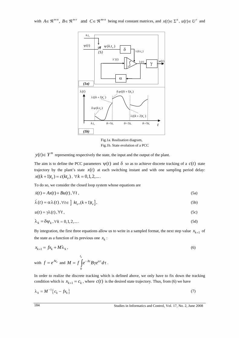
Studies in Informatics and Control, Vol. 17, No. 2, June 2008 184
with , andn n n r m nA B C× × ×∈ℜ ∈ℜ ∈ℜ being real constant matrices, and ( ) nx t ∈Σ , ( ) ru t U∈ and
( ) my t Y∈ representing respectively the state, the input and the output of the plant.
The aim is to define the PCC parameters ( )tψ and δ so as to achieve discrete tracking of a ( )c t state trajectory by the plant’s state ( )x t at each switching instant and with one sampling period delay:
(( 1) ) ( )e ex k t c kt+ = , 0,1,2,...k∀ = .
To do so, we consider the closed loop system whose equations are
( ) ( ) ( )x t Ax t Bu t= +& , t∀ , (5a)
( ) ( )t tλ = αλ& , ] ], ( 1)e et kt k t∀ ∈ + , (5b)
( ) ( )u t t= γλ , t∀ , (5c)
k kλ = δψ , 0,1, 2,...k∀ = . (5d)
By integration, the first three equations allow us to write in a sampled format, the next step value 1kx + of
the state as a function of its previous one kx :
1k k kx fx M+ = + λ , (6)
with eAtf e= and 0
etAM f e B e d− τ ατ= γ τ∫ .
In order to realize the discrete tracking which is defined above, we only have to fix down the tracking condition which is 1k kx c+ = , where ( )c t is the desired state trajectory. Thus, from (6) we have
{ }1k k kM c fx−λ = − (7)
etk.
{S}
)(tψ ).( etkψ
)(' tλ)(tλ γ ( )w t
δ
α
)(tλ
t
))1(( −+λ etk
).(. etkψδ
))2(( −+λ etk
))1((. etk +ψδ
etk. ( 1). ek t+ ( 2). ek t+ ( 3). ek t+
(1a)
(1b)
Fig.1a. Realisation diagram, Fig.1b. State evolution of a PCC
).( etkλ

Studies in Informatics and Control, Vol. 17, No. 2, June 2008 185
Equation (7) gives the switching value of the controller’s state, under the condition that 1M − exists [6]. Hence, in this case, we are able to define the PCC with
1M −δ = and ( ) ( ) ( )t c t fx tψ = − ,
2.3 Adaptation of the PCC
According to [8], it is possible to enhance the performance of a PCC by enabling switching at high frequencies, i.e. 0et
+→ . The author shows that in this case, a PCC allows control of time varying plants or even non linear systems, using state or output reference trajectories for state and output feedback respectively.
To understand the effect of fast switching, let’s rewrite the equation of the closed loop structure in the case of an output feedback:
10
etA
k k ky Cfx Cf e B e d− τ ατ+
⎧ ⎫⎪ ⎪= + γ τ λ⎨ ⎬⎪ ⎪⎩ ⎭∫ (8)
with dim( ( ))t mλ = , dim( ) m mα = × , dim( ) r mγ = × .
By realizing 0et+→ , it is possible to simplify (8) by
10
( ) ( )et
k k n n e ky x I A B I t d+
⎧ ⎫⎪ ⎪= ϒ + ϒ − τ γ + α τ λ⎨ ⎬⎪ ⎪⎩ ⎭∫ (9)
with ( )n eC I Atϒ = + and nI being the n-th order identity matrix.
We can thus write (9) as
21 ( ( ))k k e k e e ky y CAt x CB t t+ = + + γ + ε λ , (10)
2( )etε being negligible when 0et+→ .
In order to evaluate the initial condition of the PCC state at each switching instant, we fix the tracking condition as 1 ( )k o ky c+ = , where ( )oc t is the output’s desired trajectory, such that the closed loop structure becomes
2( ( )) ( )e e k o k k e kCB t t c y CAt xγ + ε λ = − − (11)
In order to solve (11) numerically, we rewrite the latter as 2( ( )) ( )k k e e k o k k e kCB t t c y CAt xλ − λ + γ + ε λ = − − (12)
With fast switching ( 0et+→ ), equation (12) becomes
( )k m k o k kI c y−λ = λ + − (13)
Note that mI − is the m-th order diagonal matrix whose non zero terms are strictly less than 1 and tend to 1.
Equation (13) can be interpreted algorithmically by an iterative evaluation of kλ at each calculation step:
( )k m k o k kI c y−λ ← λ + − (14)
The calculation of the initial condition of the PCC state at each switching instant is thus highly simplified.
Moreover, the structure of the PCC is simplified by the fact that 0et+→ . In fact, in this condition, the

Studies in Informatics and Control, Vol. 17, No. 2, June 2008 186
evolution of the controller’s state is negligible, such that the integrator setup of figure 1a acts as a Zero Order Holder (ZOH). Furthermore, if we consider that switching occur at each calculation step of a digital calculator, the ZOH can be replaced by a short circuit.
Figure 2 illustrates the structure of such a regulator.
The major advantage of this adaptation of the usual PCC is the fact that the model of the plant is unnecessary. It thus allows control of non linear systems.
3. Simulation Experiments
By means of its mathematical model, the anaerobic digestion process has been simulated in Matlab/Simulink® and controlled with the presented regulator.
Regulation of the output Q (energy supply)
The performances of the piecewise continuous control have been evaluated for step changes of :
- the set point Q∗ in the interval from 0.1 to 0.5 (Fig. 3a),
- the disturbance 0iS in the interval from 3 to 4 (Fig. 3b).
Regulation of the output S (depolution control)
In the same way, the controller’s performance has been tested with step changes of:
- the set point S∗ in the interval from 1 to 0.5 (Fig. 4a),
- the disturbance 0iS in the interval from 3 to 4 (Fig. 4b).
According to [5], the input D is limited in the interval 0 0.35D≤ ≤ in all cases.
The simulation results show that the proposed piecewise continuous controller presents very good performances of set point tracking (Figs. 3a, 4a) of a discontinuous reference trajectory. It also ensures regulation (Figs. 3b, 4b) of the plant’s output, rejecting disturbances in a large range.
)()( tutw =
)(ty
( )c to
+
-
−mI
Fig.2. Adaptation of a PCC (fast switching)
γ
+
)(tλ

Studies in Informatics and Control, Vol. 17, No. 2, June 2008 187
4. Conclusion and Future Works
Control of the anaerobic digestion process presents difficulties due to its non linear nature. However, the proposed method uses a controller, which is independent of the plant’s model, thus overcoming the non linear effects in the present working conditions. Moreover, the regulator can be very easily implemented and requires few step calculations.
0 5 10 15 20 25 30
0
0.1
0.2
0.3
0.4
0.5
0 5 10 15 20 25 30
0
0.1
0.2
0.3
0.4
0.5
0 5 10 15 20 25 30
0
0.5
1
D
Q
time, d
0 5 10 15 20 25 30-0.2
0
0.2
0.4
0.6
D
Q
Q*
time, d
Fig .3a. Step changes of set point (Q*)
Fig. 3b. Step changes of influent organics concentration (S0i)
D
S
time, d
D
S
S*
time, d
Fig. 4a. Step changes of set point (S*)
Fig. 4b. Step changes of influent organics concentration (S0i)
3
40 iS
3
40 iS

Studies in Informatics and Control, Vol. 17, No. 2, June 2008 188
As a perspective of our study, works are presently being carried out to realize control of the anaerobic digestion process with a wider range of the set points and disturbances.
ACKNOWLEDGEMENT
This work is supported by the European Union under Grants 15010/02Y0064/03-04 CAR/Presage N 4605 Obj. 2-2004:2 - 4.1 – N 160/4605.
REFERENCES
1. FORSTER, C.F., D.A. JOHN WASE, Environmental Biotechnology, Ellis Horwood Ltd, N.Y., 1990.
2. BASTIN, G., D. DOCHAIN, On-line estimation and adaptive control of bioreactors, Elsevier Science Publ., Amsterdam, 1991.
3. SIMEONOV, I., Modelling and control of anaerobic digestion of organic waste, Chem. Biochem. Eng. Q., 8, 1994, pp. 45-52.
4. SIMEONOV, I., I. QUEINNEC, Linearizing control of the anaerobic digestion with addition of acetate, Control Engineering Practice, 14, 2006, pp. 799-810.
5. SIMEONOV, I.S., Mathematical modeling and parameter estimation of anaerobic fermentation processes, Bioprocess Engineering, 21, 1999, pp. 377-381.
6. KONCAR, V., C. VASSEUR, Systèmes à fonctionnement par morceaux et poursuite échantillonnée, APII-JESA, 35, 2001, pp. 665-689.
7. KONCAR, V., C. VASSEUR, Control of linear systems using piecewise continuous systems. IEE Control Theory & Applications, 150, 2003, pp. 565-576.
8. CHAMROO, A. , Studies in Piecewise Continuous Systems: Application in Online Identification and Real Time Control Fields. Ph.D. Thesis, Université des Sciences et Technologies de Lille (in French), 2006.

Studies in Informatics and Control, Vol. 17, No. 2, June 2008 189
A Compliance Control of a Hyperredundant Robot
Mircea Ivanescu1, Mihaela Cecilia Florescu1, Nirvana Popescu2, Decebal Popescu2
1 University of Craiova, Romania
e-mail: [email protected]
2 University Politechnica Bucharest, Romania
Abstract: The grasping control problem for a hyperredundant arm is studied. First, the dynamic model of the arm is analyzed. The control problems are divided in the subproblems: the position control in a desired reaching area, the control of the arm around the object-load and the force control of grasping. The difficulties determined by the complexity of the non-linear integral-differential equations are avoided by using a very basic energy relationship of this system. First, the dynamic control of the arm for a desired reaching area is inferred. Then, the position control and the force control for grasping are discussed. Numerical simulations are presented.
Keywords: distributed parameter systems, force control, grasping, hyperredundant robots.
Mircea Ivanescu received his B.Sc. degree in Automatic Control in 1965 from the University Politehnica Bucharest. He received his Ph.D. degree in Control Systems in 1975. Now, he is a Professor at the Department of Mechatronics, University of Craiova. His research interests are focused on: Distributed Parameter Systems, Discrete Optimization Problems, Fuzzy Systems, Nonlinear Systems, and Robotics.
Mihaela Cecilia Florescu received her B. Sc. and M. Sc. degrees in Electromechanical Engineering in 1995 and 1996, respectively, from University of Craiova. Now she is a Lecturer at the Mechatronics Department, University of Craiova. Her research interests are focused on: Distributed Parameter Systems, Fuzzy Systems, and Robotics.
Nirvana Popescu received her B.Sc. and M. Sc. degrees in Computer Science in 1997 and 1998, respectively, from University Politehnica, Bucharest. She received the Ph.D. degree in Computer Science in 2003 from University Politehnica, Bucharest. Now she is a Lecturer at the Computer Department, University Politehnica, Bucharest. Her research interests are focused on: Fuzzy Systems, Digital Circuits, Intelligent Adaptive Systems, and Vision Control.
Decebal Popescu received his B. Sc. and M. Sc. degrees in Computer Science in 1997 and 1998, respectively, from University Politehnica, Bucharest. He received the Ph.D. degree in Computer Science in 2003 from University Politehnica, Bucharest. Now he is a Lecturer at the Computer Department, University Politehnica, Bucharest. His research interest is focused on: Fuzzy Systems, Digital Circuits, VLSI circuits, and Robotics.
1. Introduction
The control of a hyperredundant manipulator is very complex and a great number of researchers have tried to offer solutions for this difficult problem. In [7] it was analyzed the control by cables or tendons meant to transmit forces to the elements of the arm in order to closely approximate the arm as a truly continuous backbone. In [6], Gravagne analyzed the kinematical model of “hyper-redundant” robots, known as “continuum” robots. Important results were obtained by Chirikjian and Burdick [3, 4], which laid the foundations for the kinematical theory of hyper-redundant robots. Mochiyama has also investigated the problem of controlling the shape of an HDOF rigid-link robot with two-degree-of-freedom joints using spatial curves [11]. In [11, 14] it is presented the “state of art” of continuum robots, outline their areas of application and introduce some control issues.
The difficulty of the dynamic control is determined by integral-partial-differential models with high nonlinearities that characterize the dynamic of these systems. In [8] the dynamic model for 3D space is inferred and a control law based on the energy of the system is analyzed.
In this paper, the problem of a class of hyperredundant arms with continuum elements that performs the grasping function by coiling is discussed. The difficulties determined by the complexity of the non-linear integral-differential equations, that represent the dynamic model of the system, are avoided by using a very basic energy relationship of this system. Energy-based control laws are introduced for the position control problem. A force control method is also proposed.
The paper is organized as follows: section 2 presents the basic principles of a hyperredundant structure with continuum elements; section 3 studies the dynamic model; section 4 discusses the both problem of grasping by coiling, the position control and force control; section 5 verifies by computer simulation the control laws.
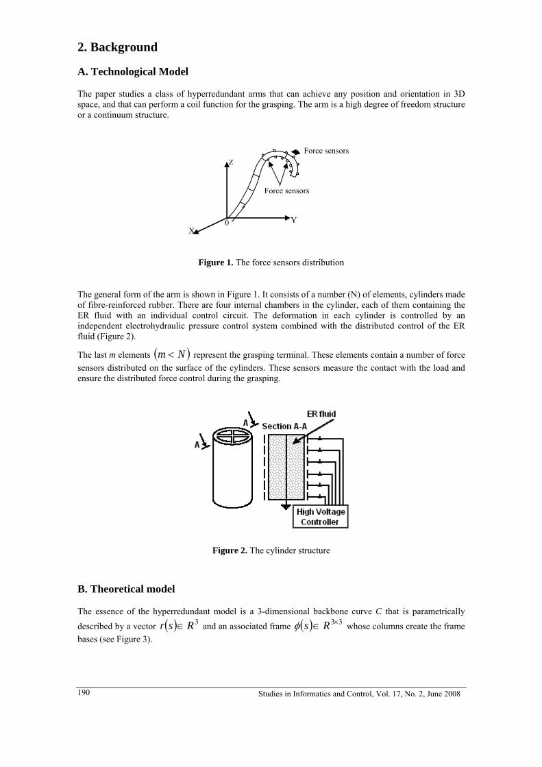
Studies in Informatics and Control, Vol. 17, No. 2, June 2008 190
2. Background
A. Technological Model
The paper studies a class of hyperredundant arms that can achieve any position and orientation in 3D space, and that can perform a coil function for the grasping. The arm is a high degree of freedom structure or a continuum structure.
Figure 1. The force sensors distribution
The general form of the arm is shown in Figure 1. It consists of a number (N) of elements, cylinders made of fibre-reinforced rubber. There are four internal chambers in the cylinder, each of them containing the ER fluid with an individual control circuit. The deformation in each cylinder is controlled by an independent electrohydraulic pressure control system combined with the distributed control of the ER fluid (Figure 2).
The last m elements ( )Nm < represent the grasping terminal. These elements contain a number of force sensors distributed on the surface of the cylinders. These sensors measure the contact with the load and ensure the distributed force control during the grasping.
Figure 2. The cylinder structure
B. Theoretical model
The essence of the hyperredundant model is a 3-dimensional backbone curve C that is parametrically described by a vector ( ) 3Rsr ∈ and an associated frame ( ) 33×∈Rsφ whose columns create the frame bases (see Figure 3).
0 YX
Z
Force sensors
Force sensors

Studies in Informatics and Control, Vol. 17, No. 2, June 2008 191
Figure 3. (a) The backbone structure; (b) The backbone parameters
The independent parameter s is related to the arc-length from the origin of the curve C, [ ]Ls ,0∈ ,
where ∑=
=N
iilL
1, where il represent the length of the elements i of the arm in the initial position.
The position vector on curve C is given by
( ) ( ) ( ) ( )[ ]Ttsztsytsxtsr ,,,, = (1)
where
( ) ( ) ( )∫ ′′′=s
sdtsqtstsx0
,cos,sin, θ (2)
( ) ( ) ( )∫ ′′′=s
sdtsqtstsy0
,cos,cos, θ (3)
( ) ( )∫ ′′=s
sdtsqtsz0
,sin, , [ ]ss ,0∈′ (4)
For an element dm, kinetic and gravitational potential energy will be:
( )222
21
zyx vvvdmdT ++= , zgdmdV ⋅⋅= (5)
where dsdm ⋅= ρ , and ρ is the mass density.
The elastic potential energy will be approximated by the bending of the element:
( )∑=
+=N
iiie qdkV
1
222
4θ (6)
We will consider ( )tsF ,θ , ( )tsFq , the distributed forces on the length of the arm that determine
motion and orientation in the θ -plane, q -plane. The mechanical work is:
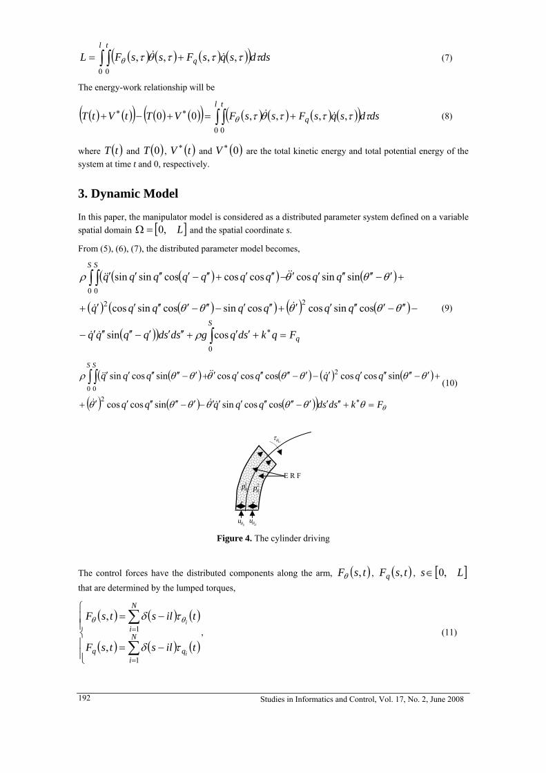
Studies in Informatics and Control, Vol. 17, No. 2, June 2008 192
( ) ( ) ( ) ( )( )∫ ∫ +=l t
q dsdsqsFssFL0 0
,,,, ττττθτθ && (7)
The energy-work relationship will be
( ) ( )( ) ( ) ( )( ) ( ) ( ) ( ) ( )( )∫ ∫ +=+−+ ∗∗l t
q dsdsqsFssFVTtVtT0 0
,,,,00 ττττθτθ && (8)
where ( )tT and ( )0T , ( )tV ∗ and ( )0∗V are the total kinetic energy and total potential energy of the system at time t and 0, respectively.
3. Dynamic Model
In this paper, the manipulator model is considered as a distributed parameter system defined on a variable spatial domain [ ]L,0=Ω and the spatial coordinate s.
From (5), (6), (7), the distributed parameter model becomes,
( )( )( ( )
( ) ( )( ) ( ) ( )
( )) q
S
S S
Fqksdqgsdsdqqqq
qqqqqqq
qqqqqqqqq
=+′′+′′′′−′′′′′−
−′′−′′′′′+′′′−′′−′′′′′+
+′−′′′′′′−′′′+′′−′′′′′
∗∫
∫ ∫
0
22
0 0
cossin
cossincoscossincossincos
sinsincoscoscoscossinsin
ρ
θθθθθ
θθθρ
&&
&&
&&&&
(9)
( )( ( ) ( ) ( )
( ) ( ) ( )) θθθθθθθθ
θθθθθθθρ
Fksdsdqqqqq
qqqqqqqqS S
=+′′′′−′′′′′′′−′−′′′′′′+
+′−′′′′′′−′−′′′′′′+′−′′′′′′
∗
∫ ∫
coscossinsincoscos
sincoscoscoscoscossincossin
2
2
0 0
&&&
&&&&&(10)
Figure 4. The cylinder driving
The control forces have the distributed components along the arm, ( )tsF ,θ , ( )tsFq , , [ ]Ls ,0∈ that are determined by the lumped torques,
( ) ( ) ( )
( ) ( ) ( )⎪⎪⎩
⎪⎪⎨
⎧
−=
−=
∑
∑
=
=N
iqq
N
i
tilstsF
tilstsF
i
i
1
1
,
,
τδ
τδ θθ
, (11)
E R F
Liθτ
iu
1θ iu
2θ
r r
2i
pθ1
ipθ

Studies in Informatics and Control, Vol. 17, No. 2, June 2008 193
where δ is Kronecker delta, llll N ==== K21 , and
( ) ( ) 821 dSpptiii
⋅−= θθθτ (12)
( ) ( ) 821 dSpptiii qqq ⋅−=τ , Ni ,,2,1 K= (13)
In (12), (13), 1i
pθ , 2i
pθ , 1iqp , 2
iqp represent the fluid pressure in the two chamber pairs, θ , q and S, d
are section area and diameter of the cylinder, respectively (Figure 4). The pressure control of the chambers is described by the equations:
( ) ki
ki
ki udt
dpa θ
θθ = (14)
( ) qki
kqi
ki udt
dpqb = , 2,1=k ; Ni ,,2,1 K= (15)
where ( )θkia , ( )qbki are determined by the fluid parameters and the geometry of the chambers and
( ) 00 >kia , ( ) 00 >kib (16)
4. Control Problem
The control problem of a grasping function by coiling is constituted from two subproblems: the position control of the arm around the object-load and the force control of grasping.
We consider that the initial state of the system is given by
( ) [ ]Tqs 000 ,,0 θωω == (17)
corresponding to the initial position of the arm defined by the curve 0C
( ) ( )( )sqsC 000 ,: θ , [ ]Ls ,0∈ (18)
The desired point is represented by a desired position of the arm, the curve dC that coils the load,
[ ]Tddd q,θω = (19)
( ) ( )( )sqsC ddd ,: θ , [ ]Ls ,0∈ (20)
Figure 5. (a) The grasping position; (b) The grasping parameters
(a)
Graspingelements
load
Initial Position
Desired Position (Cd)
Fid
X
0b Cb
s
(b)

Studies in Informatics and Control, Vol. 17, No. 2, June 2008 194
In a grasping function by coiling, only the last m elements ( )Nm < are used. Let gl be the active
grasping length, where ∑=
=n
miig ll .
We define by ( )te p the position error
( ) ( ) ( )( ) ( ) ( )( )( )∫−
−+−=L
lLbbp
g
dssqtsqstste ,, θθ (21)
It is difficult to measure practically the angles θ , q for all [ ]Ls ,0∈ . These angles can be evaluated or measured at the terminal point of each element. In this case, the relation (21) becomes
( ) ( )( ) ( )( )( )∑=
−+−=N
mibiibiip qtqtte θθ (22)
The error can also be expressed with respect to the global desired position dC
( ) ( )( ) ( )( )( )∑=
−+−=N
idiidiip qtqtte
1θθ (23)
The position control of the arm means the motion control from the initial position 0C to the desired
position bC in order to minimize the error.
A. Desired Area Reaching Control
An area reaching control problem is discussed. The desired area is specified by the inequality function:
( ) 0≤rf δ (24)
where f is a scalar function with continuous first partial derivates, 0rrr F −=δ , 30 Rr ∈ is a reference
point of the desired area and Fr is the position vector (3) of the terminal point.
The potential energy function for the area reaching control has the form [1]:
( )( )( ) ( )⎪⎩
⎪⎨⎧
>
≤= 0,
21
0,02 rfrfk
rfrV
PP δδ
δ (25)
Theorem 1. The closed-loop control system for the desired reaching area problem is stable if the control forces are
( ) ( ) ( ) ( )⎟⎟⎠
⎞⎜⎜⎝
⎛⋅
∂∂
−−−= ∗∗iiP
TP qakr
Vtektektiiiiii
,,0max2 θτθθθθθθ & (20)
( ) ( ) ( ) ( )⎟⎟⎠
⎞⎜⎜⎝
⎛⋅
∂∂
−−−= ∗∗iiP
TP
qqqq qakr
Vtektekt
iqiiiii,,0max2 θτθ & (21)
Proof. See Appendix.
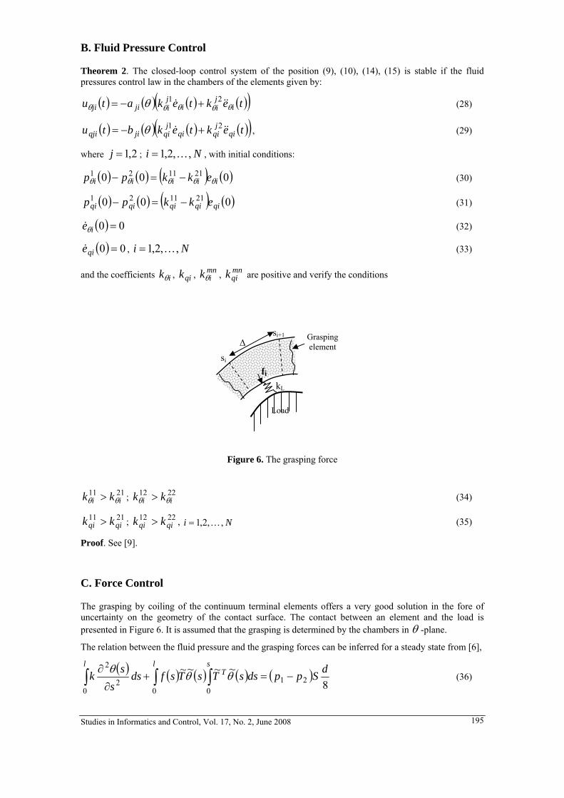
Studies in Informatics and Control, Vol. 17, No. 2, June 2008 195
B. Fluid Pressure Control
Theorem 2. The closed-loop control system of the position (9), (10), (14), (15) is stable if the fluid pressures control law in the chambers of the elements given by:
( ) ( ) ( ) ( )( )tektekatu ijii
jijiji θθθθθ θ &&& 21 +−= (28)
( ) ( ) ( ) ( )( )tektekbtu qij
qiqij
qijiqji &&& 21 +−= θ , (29)
where 2,1=j ; Ni ,,2,1 K= , with initial conditions:
( ) ( ) ( ) ( )000 211121iiiii ekkpp θθθθθ −=− (30)
( ) ( ) ( ) ( )000 211121qiqiqiqiqi ekkpp −=− (31)
( ) 00 =ieθ& (32)
( ) 00 =qie& , Ni ,,2,1 K= (33)
and the coefficients ikθ , qik , mnikθ , mn
qik are positive and verify the conditions
Figure 6. The grasping force
2111ii kk θθ > ; 2212
ii kk θθ > (34)
2111qiqi kk > ; 2212
qiqi kk > , Ni ,,2,1 K= (35)
Proof. See [9].
C. Force Control
The grasping by coiling of the continuum terminal elements offers a very good solution in the fore of uncertainty on the geometry of the contact surface. The contact between an element and the load is presented in Figure 6. It is assumed that the grasping is determined by the chambers in θ -plane.
The relation between the fluid pressure and the grasping forces can be inferred for a steady state from [6],
( ) ( ) ( ) ( ) ( )8
~~~~21
0 002
2 dSppdssTsTsfdss
skl s
Tl
−=+∂
∂∫ ∫∫ θθθ
(36)
si
si+1Δ
fi
kL
Load
Grasping element
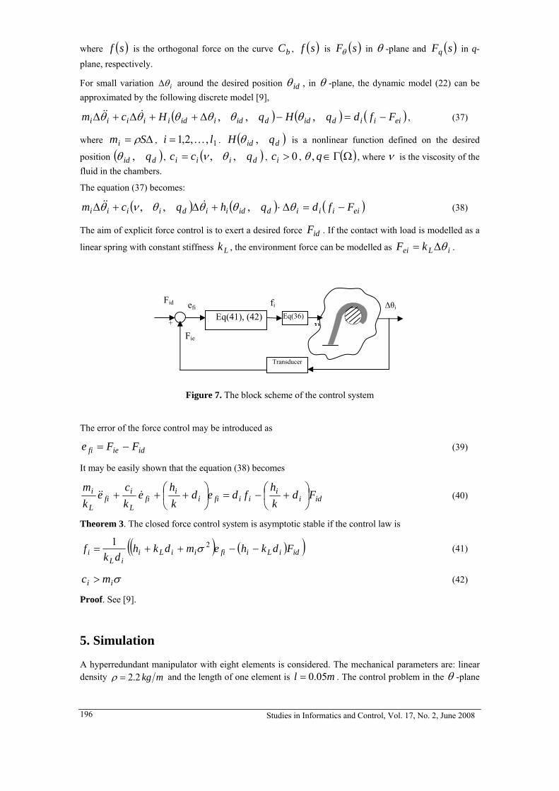
Studies in Informatics and Control, Vol. 17, No. 2, June 2008 196
where ( )sf is the orthogonal force on the curve bC , ( )sf is ( )sFθ in θ -plane and ( )sFq in q-plane, respectively.
For small variation iθΔ around the desired position idθ , in θ -plane, the dynamic model (22) can be approximated by the following discrete model [9],
( ) ( ) ( )eiiididdidiidiiiii FfdqHqHcm −=−Δ++Δ+Δ ,,, θθθθθθ &&& , (37)
where Δ= Smi ρ , 1,,2,1 li K= . ( )did qH ,θ is a nonlinear function defined on the desired
position ( )did q,θ , ( )diii qcc ,, θν= , 0>ic , ( )ΩΓ∈q,θ , where ν is the viscosity of the fluid in the chambers.
The equation (37) becomes:
( ) ( ) ( )eiiiididiidiiii Ffdqhqcm −=Δ⋅+Δ+Δ θθθθνθ ,,, &&& (38)
The aim of explicit force control is to exert a desired force idF . If the contact with load is modelled as a
linear spring with constant stiffness Lk , the environment force can be modelled as iLei kF θΔ= .
Figure 7. The block scheme of the control system
The error of the force control may be introduced as
idiefi FFe −= (39)
It may be easily shown that the equation (38) becomes
idii
iifiii
fiL
ifi
L
i Fdkh
fdedkh
ekc
ekm
⎟⎠
⎞⎜⎝
⎛ +−=⎟⎠
⎞⎜⎝
⎛ +++ &&& (40)
Theorem 3. The closed force control system is asymptotic stable if the control law is
( ) ( )( )idiLifiiiLiiL
i Fdkhemdkhdk
f −−++= 21 σ (41)
σii mc > (42)
Proof. See [9].
5. Simulation
A hyperredundant manipulator with eight elements is considered. The mechanical parameters are: linear density mkg2.2=ρ and the length of one element is ml 05.0= . The control problem in the θ -plane
Fid
Eq(41), (42)efi fi
Eq(36) υ
Δθi
+
Fie
Transducer

Studies in Informatics and Control, Vol. 17, No. 2, June 2008 197
will be analyzed. The initial position is the defined by ( ) ⎟⎠⎞
⎜⎝⎛ =
2: 00
πθ sC . First, a reaching desired area
control is introduced where the area is defined by the circle ( ) ( ) 220 Rrrr −−=δϕ , ( )2,30 =r ,
1=R and the control law (20) is applied. The position error rΔ is computed and the phase error is presented in Figure 8. Then, the grasping function is performed for a circular load defined by
( ) ( ) ( )220
20: ∗∗∗∗∗ =−+− ryyxxCb , where ( )∗∗ yx , represent the coordinates in θ -plane. A
discretisation for each element with an increment 3l=Δ is introduced. A control law (28) is used. The result is presented in Figure 9.
Figure 8. The position error phase portrait
-2 -1 0 1 2 3 4 5 6 70
1
2
3
4
5
6
7
Position Control in THETA Plane
Load
Arm Positions
Figure 9. The position control
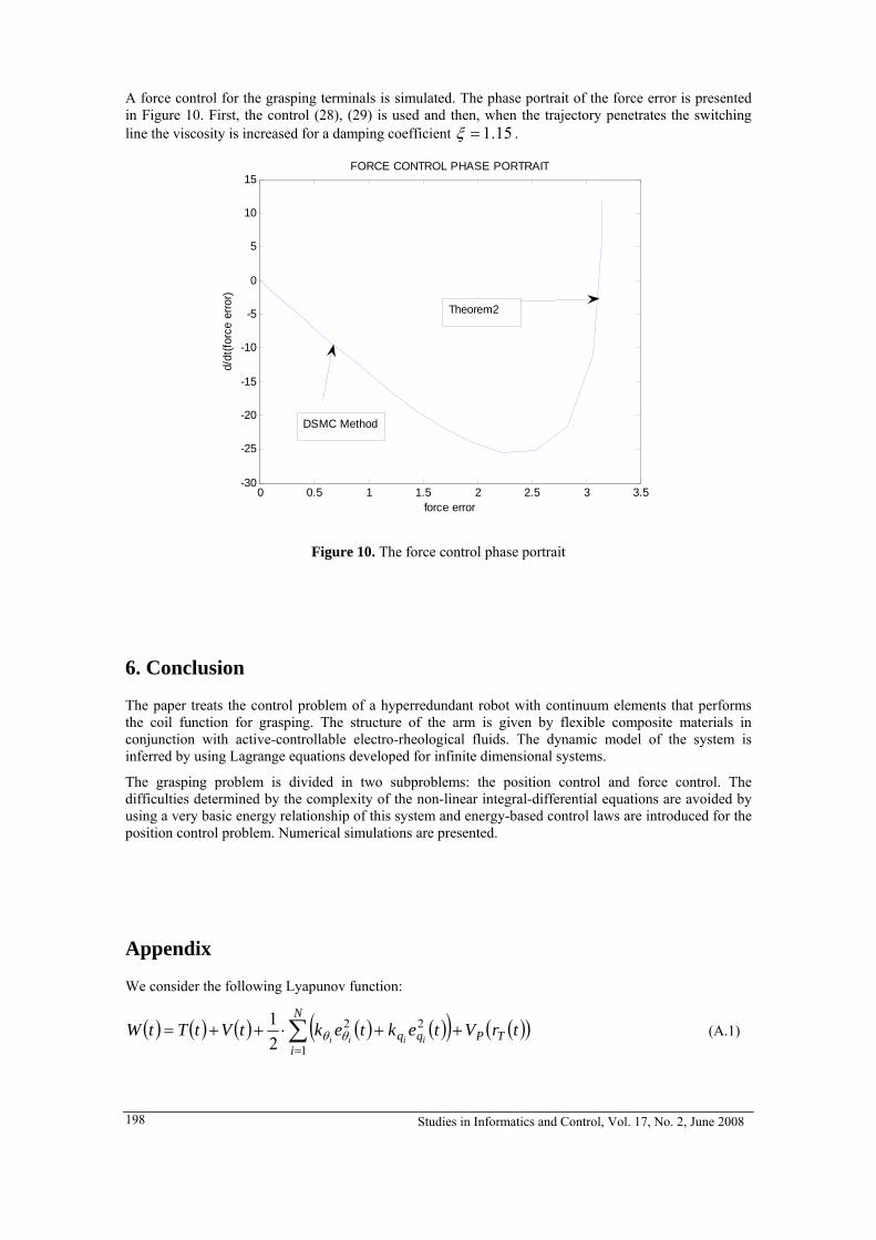
Studies in Informatics and Control, Vol. 17, No. 2, June 2008 198
A force control for the grasping terminals is simulated. The phase portrait of the force error is presented in Figure 10. First, the control (28), (29) is used and then, when the trajectory penetrates the switching line the viscosity is increased for a damping coefficient 15.1=ξ .
0 0.5 1 1.5 2 2.5 3 3.5-30
-25
-20
-15
-10
-5
0
5
10
15
force error
d/dt
(forc
e er
ror)
FORCE CONTROL PHASE PORTRAIT
Theorem2
DSMC Method
Figure 10. The force control phase portrait
6. Conclusion
The paper treats the control problem of a hyperredundant robot with continuum elements that performs the coil function for grasping. The structure of the arm is given by flexible composite materials in conjunction with active-controllable electro-rheological fluids. The dynamic model of the system is inferred by using Lagrange equations developed for infinite dimensional systems.
The grasping problem is divided in two subproblems: the position control and force control. The difficulties determined by the complexity of the non-linear integral-differential equations are avoided by using a very basic energy relationship of this system and energy-based control laws are introduced for the position control problem. Numerical simulations are presented.
Appendix
We consider the following Lyapunov function:
( ) ( ) ( ) ( ) ( )( ) ( )( )∑=
++⋅++=N
iTPqq trVtektektVtTtW
iiii1
22
21
θθ (A.1)

Studies in Informatics and Control, Vol. 17, No. 2, June 2008 199
where T, V represent the kinetic and potential energies of the system. ( )tW is positive definite because
the terms that represent the energy T and V are always ( ) 0≥tT , ( ) 0≥tV .
By using (19), the derivative of this function will be:
( )
( ) ( )( ) ( ) ( ) ( ) ( )
( )
( )
( )
( )∑=
∗
∗
∗
∗
⎟⎟⎟⎟⎟
⎠
⎞
⎜⎜⎜⎜⎜
⎝
⎛
⎟⎟⎟
⎠
⎞
⎜⎜⎜
⎝
⎛
⎟⎟⎟
⎠
⎞
⎜⎜⎜
⎝
⎛
+
+
∂∂
+⎟⎟⎟
⎠
⎞
⎜⎜⎜
⎝
⎛
⎟⎟⎟
⎠
⎞
⎜⎜⎜
⎝
⎛
+
+
∂∂
+
++++
=N
iiiq
iiPTP
ii
iiPTP
qqqiqi
qbk
qak
rV
qbk
qak
rV
tetektetekqtt
tW
i
iq
i
i
iiiiiiii
1,
,,0max
,
,,0max
θ
θ
θ
θ
τθτ
θ
θθθθ
θ
&&&&
& (A.2)
For a constant desired position idθ ,
idq , from (20)-(21), the relation (A.2) can be rewritten as:
( ) ( ) 01
22 ≤+−= ∑=
∗∗N
iiqi qkktW
ii&&& θθ (A.3)
and, from [1], the closed-loop system defined by (20) converges to the desired position idi θθ → ,
idi qq → and the terminal point Fr converges to the desired area ( ) 0≤rf δ as ∞→t .
REFERENCES
1. CEAH, C.C., D.Q. WANG, Region Reaching Control of Robots: Theory and Experiments, Proceedings of IEEE International Conference on Robotics and Automation, Barcelona, 2005, pp. 986-991.
2. CHIAVERINI, S., B. SICILIANO, L. VILLANI, Force and Position Tracking: Parallel Control with Stiffness Adaptation, IEEE Control Systems, Vol. 18, No. 1, 1996, pp. 27-33.
3. CHIRIKJIAN, G. S., J. W. BURDICK, An Obstacle Avoidance Algorithm for Hyper-redundant Manipulators, Proc. IEEE International Conference on Robotics and Automation, Cincinnati, Ohio, May 1990, pp. 625 - 631.
4. CHIRIKJIAN, G.S., J. W. BURDICK, Kinematically Optimal Hyperredundant Manipulator Configurations, IEEE Transaction Robotics and Automation, Vol. 11, No. 6, Dec. 1995, pp. 794-798.
5. GE, S.S., T.H. LEE, G. ZHU, Energy-Based Robust Controller Design for Multi-Link Flexible Robots, Mechatronics, No. 7, Vol. 6, 1996, pp. 779-798.
6. GRAVAGNE, IAN A., IAN D. WALKER, On the Kinematics of Remotely - Actuated Continuum Robots, Proc. IEEE International Conference on Robotics and Automation, San Francisco, April 2000, pp. 2544-2550.
7. HEMAMI, A., Design of Light Weight Flexible Robot Arm, Robots 8 Conference Proceedings, Detroit, USA, June 1984, pp. 1623-1640.
8. IVANESCU, M., Position Dynamic Control for a Tentacle Manipulator, Proc. IEEE International Conference on Robotics and Automation, Washington, A1-15, May 2002, pp. 1531-1539.
9. IVANESCU,M., M.C. FLORESCU, N. POPESCU, D. POPESCU, Position and Force Control of the Grasping Function for a Hyperredundant Arm, Proc. of IEEE International Conference on Robotics and Automation, Pasadena, California, 2008 (to be published).

Studies in Informatics and Control, Vol. 17, No. 2, June 2008 200
10. MOCHIYAMA, H., H. KOBAYASHI, The Shape Jacobian of a Manipulator with Hyper Degrees of Freedom, Proc. 1999 IEEE International Conference on Robotics and Automation, Detroit, May 1999, pp. 2837- 2842.
11. MOCHIYAMA, H., E. SHIMEURA, H. KOBAYASHI, Direct Kinematics of Manipulators with Hyper Degrees of Freedom and Serret-Frenet Formula, Proc. IEEE International Conference on Robotics and Automation, Leuven, Belgium, May 1998, pp. 1653-1658.
12. ROBINSON,G., J.B.C. DAVIES, Continuum Robots – A State of the Art, Proc. 1999 IEEE International Conference on Robotics and Automation, Detroit, Michigan, May 1999, pp. 2849-2854.
13. SINGH, S.K., D.O. POPA, An Analysis and Some Fundamental Problems in Adaptive Control of Force, IEEE Transaction on Robotics and Automation, Vol. 11, No. 6, pp. 912-922.
14. SUZUMORI, K., S. IIKURA, H. TANAKA, Development of Flexible Microactuator and Its Application to Robot Mechanisms, IEEE International Conference on Robotics and Automation, Sacramento CA, April 1991, pp. 1564 - 1573.

A Digital Flatness-based Control System of a DC Motor Mounir Ayadi, Jospeh Haggège, Soufiène Bouallègue and Mohamed Benrejeb
Research Unit LARA Automatique, ENIT
BP 37, le Belvédère, 1002 Tunis, Tunisia
{mounir.ayadi, joseph.haggege, mohamed.benrejeb}@enit.rnu.tn
Abstract: In this paper, an approach to design and implement a real-time system based on a RISC microcontroller dedicated to a DC motor speed control, is proposed. A polynomial RST controller based on the flatness property of linear systems is implemented in C/C++ embedded programming language. The flatness property is used in order to design a robust controller with high performance in terms of tracking. The proposed controller is then applied to control a DC motor. The simulation and experimental results underline the efficiency of the flatness-based polynomial controller in a real-time control framework.
Keywords: Flatness control, RST polynomial controller, robustness, trajectory planning and tracking, microcontroller, AC-DC power converter.
Mounir Ayadi graduated from Ecole Nationale d’Ingénieurs de Tunis in 1998 and received his PhD degree in Automatic Control from the Institut National Polytechnique de Toulouse in 2002. He was a post-doctoral fellow at the Ecole Supérieure d’Ingénieurs en Génie Electrique de Rouen in 2003. He is currently Maître-Assistant at the Ecole Nationale d’Ingénieurs de Tunis. His research interests are in the area of control system theory, predictive and adaptive control, and flat systems.
Joseph Haggège graduated from Ecole Nationale d’Ingénieurs de Tunis and received the PhD degree in Electrical Engineering in 1998 and 2003, respectively. He is currently Maître-Assistant at the Ecole Nationale d’Ingénieurs de Tunis. His research interests are in the area of fuzzy, neural and neuro-fuzzy control, and embedded systems.
Soufiène Bouallègue received the Engineer Diploma degree in Electrical Engineering and the Master in Automatic Control from Ecole Nationale d’Ingénieurs de Tunis in 2006 and 2007, respectively.
Mohamed Benrejeb has obtained the Diploma of “Ingénieur IDN” (French “Grande Ecole”) in 1973, the Master degree of Automatic Control in 1974, the PhD in Automatic Control of the University of Lille in 1976 and the DSc of the same University in 1980. He is currently a full Professor at the Ecole Nationale d’Ingénieurs de Tunis and an invited Professor at the Ecole Centrale de Lille. His research interests are in the area of analysis and synthesis of complex systems based on classical and non conventional approaches.
1. Introduction
The possibility of varying or reversing the rotation speed of motors constitutes a necessity in industrial domain and in process automation. In this framework, the use of a DC motor can be a good solution. However, the speed control presents some delicate problems, particularly in terms of robustness, of perturbation rejection and especially when tracking trajectory. In this case, it is interesting to consider adequate control laws for the drive. Several techniques of control theory systems using conventional and non conventional methods have been applied on such type of motor [16][22][24][28].
The flatness property, introduced in 1992, presents a new point of view in the control theory domain [1-10]. This property, developed initially in the nonlinear continuous-time case, defines a class of systems well known as flat systems. The existence of a variable called flat or linearizing output allows to define all other system variables. In the linear case [3][4], it is sufficient to consider the Brunovsky's outputs of the canonical controllability form like the flat outputs [30][31]. Thus, the dynamic of such a process can be deduced without solving differential equations. Therefore, it is possible to express the state, as well as the input system, as differential functions of the flat output. The main contribution of the flatness that will be exploited in this paper is the effective trajectory planning and tracking solutions with high performances specification.
The flatness property of DC motor model will be used to obtain of a closed-loop system with high performances by designing a robust polynomial RST controller with an argued choice for its design. The tracking of a reference trajectory, function of the flat output system, as well as the rejection of disturbances and noises of measure, will be the goal of this controller.
On the other hand, the evolutions in the micro-electronics field, especially in the domain of digital signals processors are at the origin of many progresses in power electronics. Many works in the control theory domain have shown the performances of DSP (Digital Signal Processor) integration, microcontrollers (PIC, AVR...) or as digital components like FPGA or ASIC. The development of built-in digital controller on programmable target PIC 16F876 presents an advantage of fast real-time implementation of the
Studies in Informatics and Control, Vol. 17, No. 2, June 2008 201
control algorithms as well as the reduction in terms of components number and bulk [12-14].
In this paper, an approach to design such a control system as well as its hardware architecture is presented. A software integration of the developed RST algorithm, relative to the computer tools bound to this type of built-in circuits in embedded programming C/C++ language is implemented in a real-time environment.
2. Central Algorithm
2.1. Flatness-based control
The dynamic linear discrete system can be represented by equation (1) where the signals and ku ky represent the discrete systems input and output, respectively:
( ) ( )k kA q y B q u= (1)
In this equation, the polynomials ( )A q and ( )B q are the denominator and the numerator of
the transfer function respectively:
( )( )
11 1
11 1 0
n nn
nn
0A q q a q a q a
B q b q b q b
−−
−−
= + + + +
= + + +
K
K (2)
where q is the forward operator.
Applied in a real-time framework on industrial processes [5-10], the flatness property consists in designing a control signal that allows to the flat output system to track asymptotically a desired
trajectory . The discrete flat output is related to the control signal and to the output system ku kz
dkz kz ku ky
by the following relations:
( )( )
k
k k
u A q z
y B q z
=
=k
+
(3)
The flatness-based control law can be then given by the following expression:
( )1 1
0 0
n nd d
k k n i k i k i i k ii i
u z k z z a z− −
+ + += =
= + − +∑ ∑ (4)
which can be rewritten in the following polynomial expression:
( ) ( ) ( )( )dk ku K q z A q K q z= + − k (5)
The tracking error dynamics is defined by the choice of the coefficients of the ik ( )K q polynomial given by:
( ) 11 1
n nnK q q k q k q k−−= + + + +K 0
)1−
(6)
which must be Hurwitz [7].
2.2. Flatness-based RST controller
To design a polynomial controller in a linear case, we are going to follow the method given in [5] [6]. The proposed method is based on the design of a direct observer of the flat output and its forward values.
By considering the state vector of the controllable LUENBERGER
realization of system (3), the system of the equations (3), in which the variable is the partial state [30],
( 1T
k k k k nZ z z z+ += K
kz
Studies in Informatics and Control, Vol. 17, No. 2, June 2008 202
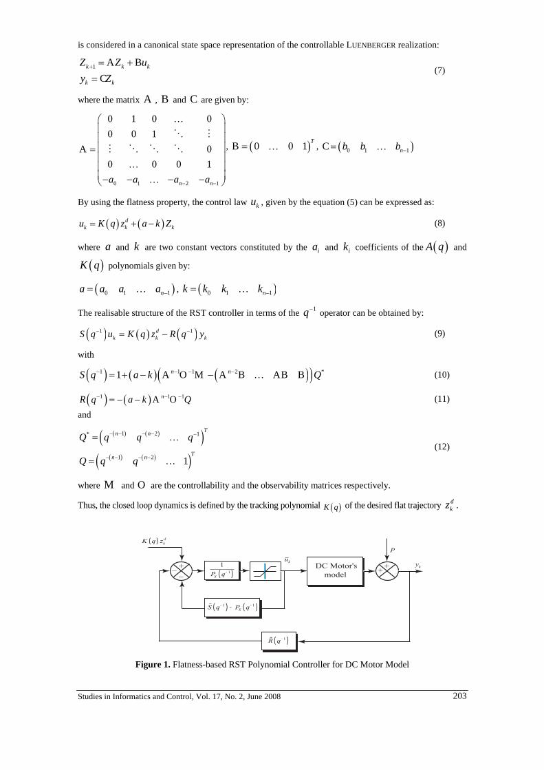
is considered in a canonical state space representation of the controllable LUENBERGER realization:
1k k
k k
kZ Z uy Z
+ = +=
A BC
(7)
where the matrix A , and C are given by: B
0 1 2 1
0 1 0 00 0 1
00 0 0 1
n na a a a− −
⎛ ⎞⎜ ⎟⎜ ⎟⎜ ⎟=⎜ ⎟⎜ ⎟⎜ ⎟− − − −⎝ ⎠
K
O M
M O O O
K
K
A ( )0 0 T= K, B , 1 ( )0 1 1nb b b −= KC
k
By using the flatness property, the control law , given by the equation (5) can be expressed as: ku
( ) ( )dk ku K q z a k Z= + − (8)
where and are two constant vectors constituted by the and coefficients of thea k ia ik ( )A q and
polynomials given by: ( )K q
( )0 1 1na a a a −= K , ( )0 1 1nk k k k −= K
The realisable structure of the RST controller in terms of the 1q− operator can be obtained by:
( ) ( ) ( )1 dk kS q u K q z R q y− = − 1
k− (9)
with
( ) ( ) ( )( )1 1 1 21 n nS q a k Q− − − −= + − − KA O M A B AB B *
1 1
(10)
( ) ( )1 nR q a k− = − − A O Q− − (11)
and
( ) ( )( )( ) ( )( )
1 2* 1
1 2 1
Tn n
Tn n
Q q q q
Q q q
− − − − −
− − − −
=
=
K
K
(12)
where M and O are the controllability and the observability matrices respectively.
Thus, the closed loop dynamics is defined by the tracking polynomial ( )K q of the desired flat trajectory . dkz
+_ +_
K q zkd( )
P
yk+uk
�R q -( )1
�S q P qS
- -( ) - ( )1 1
11P qS
-( )DC Motor's
model
Figure 1. Flatness-based RST Polynomial Controller for DC Motor Model
Studies in Informatics and Control, Vol. 17, No. 2, June 2008 203
In order to obtain a robust controller, we must introduce in the model equation (3), the pre-specified parts and , given by equation (13). In [32], it is shown that the polynomial is used to eliminate
the high frequency noises on the input signal and the polynomial to allow the rejection of static disturbance present on the output signal.
SH RH RH
SH
( )( )
1 1
1 1
1
1
S
R
H q q
H q q
− −
− −
= −
= + (13)
While taking into account the pre-specified parts and , the polynomials of the re-calculated RST controller can be seen as in equation (14).
SH RH
( ) ( ) ( )( ) ( ) ( )
1 1
1 1
S
R
S q H q S q 1
1R q H q R q
− −
− −
=
=
%
%
−
− (14)
The additive static disturbances lead generally to the increase of the control signal magnitude applied to the system exceeding admissible values. The actuator saturation can have an adverse effect upon the behaviour of the control signal and, in particular, when the controller contains an integrator [32]. Thus, the use of an anti-windup technique is mandatory.
Let's note by and the lower and higher limits of the control saturation, respectively. The effective control law applied to the plant becomes:
infsatu sup
satu
inf sup
inf sup
sup inf
ififif
k sat k sat
k sat k sat
sat k sat
u u u uu u u u
u u u
⎧ ≤ ≤⎪= ⎨⎪ <⎩
> (15)
It is also possible to impose a specified dynamics when the system leaves the saturation. The desired dynamics is defined by the polynomial ( )1
SP q− given by equation:
( )1 1 exp eS
sat
TP q qτ
− ⎛ ⎞= − −⎜ ⎟
⎝ ⎠1− (16)
where and eT satτ represent respectively the sampling period and the time constant of a first order system both chosen equal to 10 ms in the DC motor's case.
The new control law of the flatness-based polynomial controller in presence of saturation will be given by the following complete algorithm:
( ) ( ) ( ) ( )1 1 11expd e
S k k ksat
TkP q u K q z R q y S q u
τ− − −
−
⎛ ⎞⎛ ⎞= − − + −⎜ ⎜ ⎟⎜ ⎝ ⎠⎝ ⎠
% ⎟⎟ (17)
The polynomial ( 1S q− ) which introduces delays into the control signal, is given by:
( ) ( )1 11S q q S q− −= +% 1− (18)
Thus, this digital control algorithm takes into account the presence of a disturbance due to the load as well as to effects of saturation.
As in [32], the sensitivity functions which used to study the robustness of the designed RST controller are given by:
( ) ( ) ( )( )
1 11
1yp
A q S qS q
K q
− −−
−=
% (19)
Studies in Informatics and Control, Vol. 17, No. 2, June 2008 204
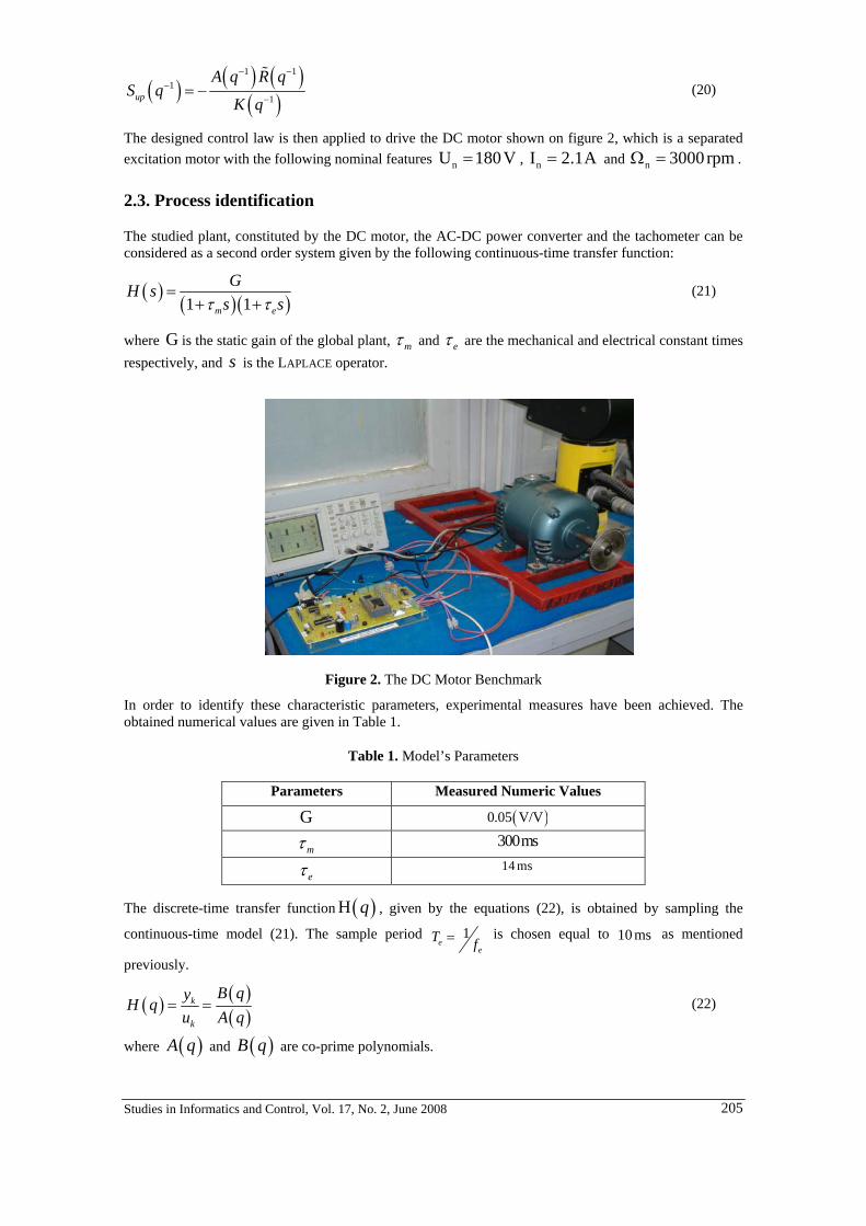
( ) ( ) (( )
)1 11
1up
A q R qS q
K q
− −−
−= −
% (20)
The designed control law is then applied to drive the DC motor shown on figure 2, which is a separated excitation motor with the following nominal features nU 180V= , nI 2.1A= and . n 3000 rpmΩ =
2.3. Process identification
The studied plant, constituted by the DC motor, the AC-DC power converter and the tachometer can be considered as a second order system given by the following continuous-time transfer function:
( ) ( )( )1 1m e
GH ss sτ τ
=+ +
(21)
where G is the static gain of the global plant, mτ and eτ are the mechanical and electrical constant times respectively, and is the LAPLACE operator. s
Figure 2. The DC Motor Benchmark
In order to identify these characteristic parameters, experimental measures have been achieved. The obtained numerical values are given in Table 1.
Table 1. Model’s Parameters
Parameters Measured Numeric Values
G ( )0.05 V/V
mτ 300ms
eτ 14 ms
The discrete-time transfer function , given by the equations (22), is obtained by sampling the
continuous-time model (21). The sample period
( )H q1
ee
T f= is chosen equal to 10 as mentioned
previously.
ms
( ) ( )( )
k
k
B qyH qu A q
= = (22)
where ( )A q and are co-prime polynomials. ( )B q
Studies in Informatics and Control, Vol. 17, No. 2, June 2008 205
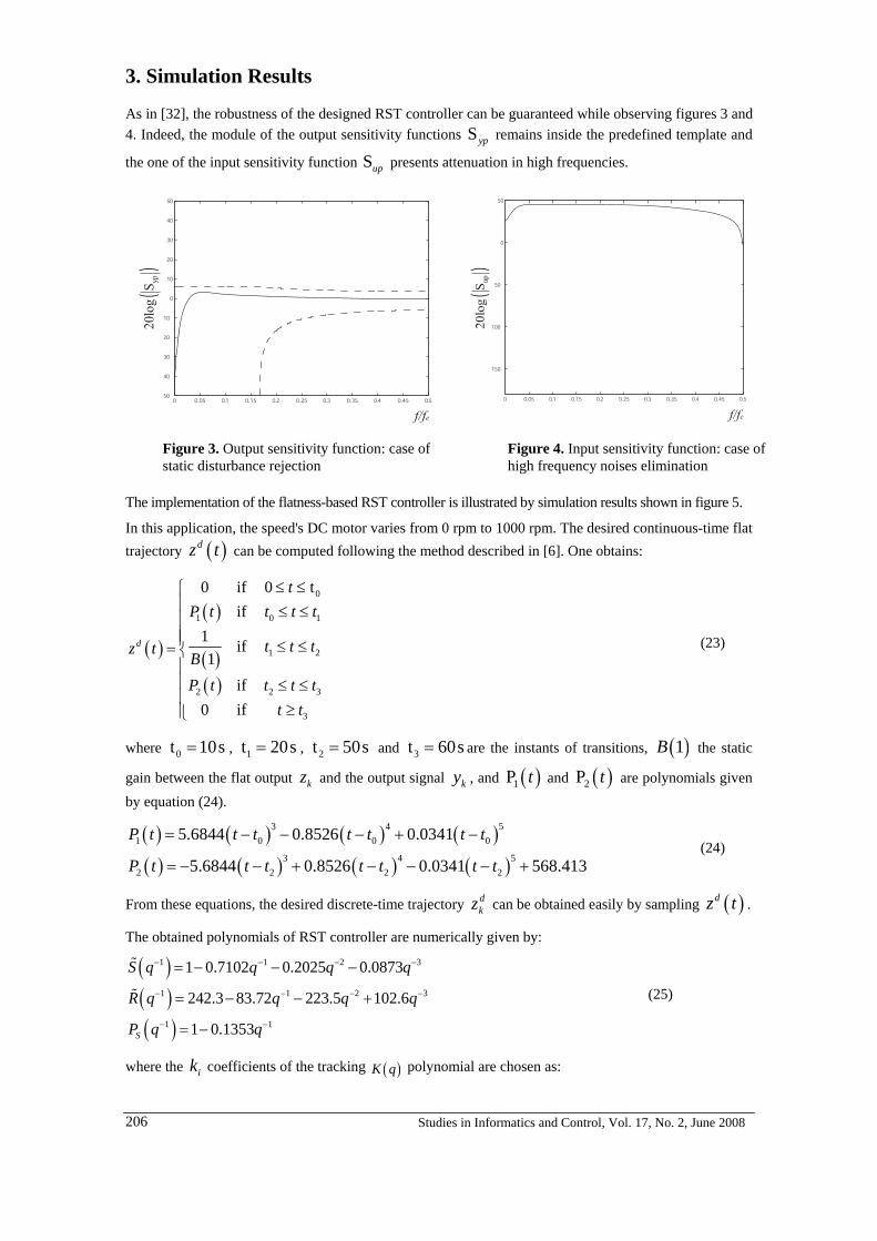
3. Simulation Results
As in [32], the robustness of the designed RST controller can be guaranteed while observing figures 3 and 4. Indeed, the module of the output sensitivity functions Syp remains inside the predefined template and
the one of the input sensitivity function presents attenuation in high frequencies. Sup
0 0.05 0.1 0.15 0.2 0.25 0.3 0.35 0.4 0.45 0.550
40
30
20
10
0
10
20
30
40
50
f/fe
20
log
Syp
()
0 0.05 0.1 0.15 0.2 0.25 0.3 0.35 0.4 0.45 0.5
150
100
50
0
50
f/fe
20lo
gS
up
()
Figure 3. Output sensitivity function: case of static disturbance rejection
Figure 4. Input sensitivity function: case of high frequency noises elimination
The implementation of the flatness-based RST controller is illustrated by simulation results shown in figure 5.
In this application, the speed's DC motor varies from 0 rpm to 1000 rpm. The desired continuous-time flat trajectory ( )dz t can be computed following the method described in [6]. One obtains:
( )
( )
( )( )
0
1 0
1
2 2
3
0 if 0 tif
1 if1
if0 if
d
tP t t t t
t t tz t BP t t t t
t t
≤ ≤⎧⎪ ≤ ≤⎪⎪⎪ ≤ ≤= ⎨⎪⎪ ≤ ≤⎪
≥⎪⎩
1
2
3
= 1t 20= 2t 50s= s
(23)
where , , and 0t 10s s 3t 60= are the instants of transitions, ( )1B the static
gain between the flat output and the output signal kz ky , and ( )1P t and ( )2P t are polynomials given by equation (24).
( ) ( ) ( ) ( )( ) ( ) ( ) ( )
3 4 51 0 0 0
3 4 52 2 2 2
5.6844 0.8526 0.0341
5.6844 0.8526 0.0341 568.413
P t t t t t t t
P t t t t t t t
= − − − + −
= − − + − − − + (24)
From these equations, the desired discrete-time trajectory can be obtained easily by sampling dkz ( )dz t .
The obtained polynomials of RST controller are numerically given by:
( )( )( )
1 1 2
1 1 2
1 1
1 0.7102 0.2025 0.0873
242.3 83.72 223.5 102.6
1 0.1353S
S q q q q 3
3R q q q
P q q
− − −
− − −
− −
= − − −
= − − +
= −
%
% q
−
− (25)
where the coefficients of the tracking ik ( )K q polynomial are chosen as:
Studies in Informatics and Control, Vol. 17, No. 2, June 2008 206
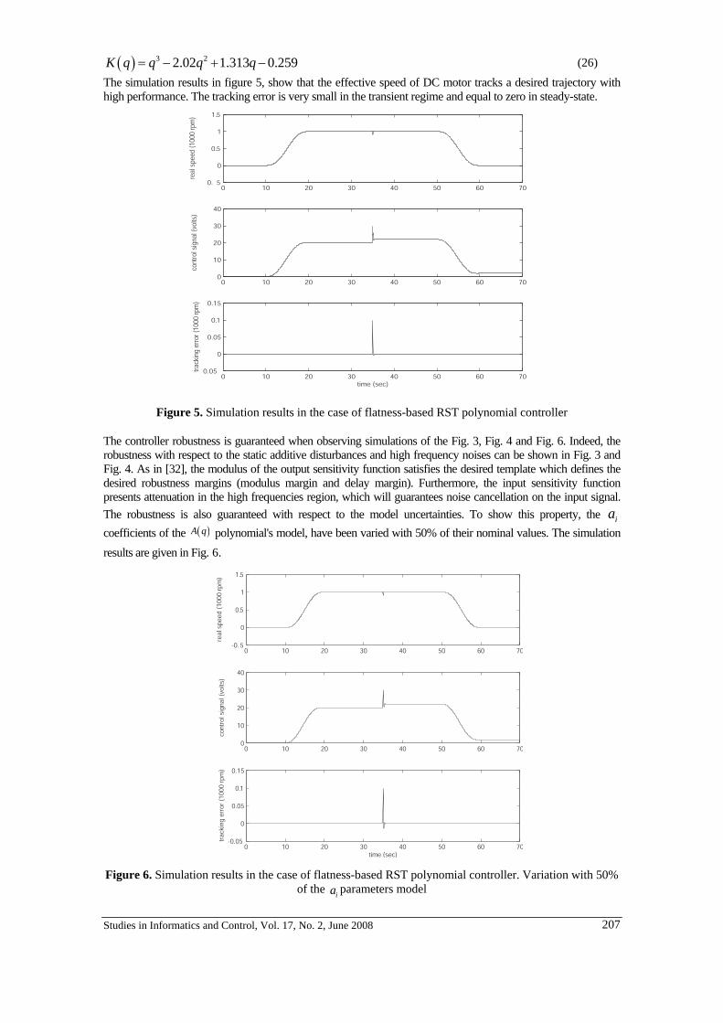
( ) 3 22.02 1.313 0.259K q q q q= − + − (26) The simulation results in figure 5, show that the effective speed of DC motor tracks a desired trajectory with high performance. The tracking error is very small in the transient regime and equal to zero in steady-state.
0 10 20 30 40 50 60 700. 5
0
0.5
1
1.5
real
spe
ed (1
000
rpm
)
0 10 20 30 40 50 60 700
10
20
30
40
cont
rol s
igna
l (vo
lts)
0 10 20 30 40 50 60 700.05
0
0.05
0.1
0.15
time (sec)
track
ing
erro
r (10
00 rp
m)
Figure 5. Simulation results in the case of flatness-based RST polynomial controller
The controller robustness is guaranteed when observing simulations of the Fig. 3, Fig. 4 and Fig. 6. Indeed, the robustness with respect to the static additive disturbances and high frequency noises can be shown in Fig. 3 and Fig. 4. As in [32], the modulus of the output sensitivity function satisfies the desired template which defines the desired robustness margins (modulus margin and delay margin). Furthermore, the input sensitivity function presents attenuation in the high frequencies region, which will guarantees noise cancellation on the input signal. The robustness is also guaranteed with respect to the model uncertainties. To show this property, the coefficients of the
ia( )A q polynomial's model, have been varied with 50% of their nominal values. The simulation
results are given in Fig. 6.
0 10 20 30 40 50 60 70-0. 5
0
0.5
1
1.5
real
spe
ed (
1000
rpm
)
0 10 20 30 40 50 60 700
10
20
30
40
cont
rol s
igna
l (vo
lts)
0 10 20 30 40 50 60 70-0.05
0
0.05
0.1
0.15
time (sec)
trac
king
err
or (
1000
rpm
)
Figure 6. Simulation results in the case of flatness-based RST polynomial controller. Variation with 50% of the parameters model ia
Studies in Informatics and Control, Vol. 17, No. 2, June 2008 207

After the simulation phase, the proposed digital control algorithm will be applied in the real-time framework.
4. Design Aspects
4.1. Digital control system hardware
Starting from the idea consisting in varying the supply voltage of the motor, several arguments led us to choose a structure of hardware control system based on an AC-DC one phase asymmetric rectifier [17][22][23][24][26][27][29].
Presently, the choice of such a converter rather than another solution, as DC-DC converter for example, is based essentially on the possibility to vary the supply motor voltage from 0V to 250V while directly using the one phase distribution network as alternative voltage source. Such an interval of variation is very sufficient to satisfy our needs since the machine to drive requires 180V as nominal supply voltage.
The present AC-DC converter, based on thyristors, represents only the power circuit of the developed hardware control system. For the thyristors's gate control circuit, a digital control based on a RISC microcontroller PIC16F876 produced by MICROCHIP, is used [12].
Control Signal
Gate Impulses
(thyristors firing angle)
Interfacing
of AC-DC converter control
and galvanic insulation
Interfacing
of acquirement and adaptation
of speed DC motor
D1 D2
Th1 Th2
measured output system
Set point
PIC16F876
microcontroller
Digital
Controller
A
C S
ourc
e
Excitation
Circuit
DC
motor
tachometer
Figure 7. Hardware Architecture of the Digital Control System
This microcontroller will be the framework for the implantation of the designed control algorithm in order to generate gate impulses control signal for the thyristors. The choice of the PIC microcontroller is justified by the simplicity of implementation, using a flexible embedded programming language such C/C++, in addition to a material architecture of peripherals allowing to satisfy integration constrains of control for an electrical system.
In order to complete the structure of the hardware control system of the separated excitation DC drive, two other hardware modules are designed: a circuit of acquisition and conditioning of the speed measurement, and a circuit providing the excitation of the DC motor. Thus, the complete architecture of the proposed hardware control system is given in Fig. 7.
4.2. AC-DC power converter control
This electronic control interface is designed and developed around an impulse transformer [16][18][20][21][23][25][26][27] which allows to control by gate impulses, the BT152 thyristors used in
Studies in Informatics and Control, Vol. 17, No. 2, June 2008 208

the bridge rectifier, while ensuring a galvanic insulation between the control circuit, based on the PIC microcontroller, and the power circuit. The use of the impulse transformer in this application, instead of optocouplers for example, is due to the possibility of working in the high frequencies and possibility to provide an important current able to fire the considered thyristors, as well as the good behaviour with high voltage and the simplicity of the use. The principle of the control circuit is given in Fig. 8.
R4R1
R2
R3
D1
D2
D3
R5
R6
Th2
Th1
Tr1
Tr2
Impulses
Transformer
+Vcc
Gate Impulses
from PIC16F876
.
.
.
DC motor
.. Alternative
Voltage Source
D1D1 D2D2
.
. .
Figure 8. AC-DC Power Converter Control
4.3. The microcontroller
In order to fire the BT152 thyristors, the used microcontroller PIC16F876 must provide the control signal as gate impulses [12-14].
The PIC microcontroller includes several variants. Indeed, the PIC16F876 is chosen because it has the necessary peripherals to implement the control algorithm. In addition, this type of microcontroller can operate with clock frequencies up to 20 MHz, improving performances of the digital controller in terms of speed signal processing.
The various peripherals considered in our application are given in the following section.
4.3.1. Timer1
Through registers T1CON, INTCON, PIE1 and TMR1 [12], the timer1 is configured to operate as a 16-bit counter which can increment from 0x0000 to 0xFFFF. With 4 MHz quartz and 1:8 prescale value, a 8 sμ clock signal is obtained.
The content of the timer1, which is the value of registers TMR1H and TMR1L, represents the value of the thyristors firing angle. As the timer 1 will be launched at each occurrence of the external interrupt that finished when the AC supply voltage crosses the zero, every 10 ms, this time can count until 1250, corresponding to angle variation from 0° to 180°. Then, one must load the content of registers TMR1H and TMR1L by the value (64285+Alpha) where Alpha takes a numerical value between 0 and 1250. Thus, the timer1 will count from the value (64285+Alpha) to 65536 to represent the angle α of thyristor firing. An interruption, flag TMR1IF, will be set when timer1 overflows, in order to start the timer0.
4.3.2. Timer0
The role of the timer0 is to generate the gate impulses used for firing SCR after the delay given by the timer1. It is an 8-bit peripheral configured in a mode through the associated registers [12]. With the same 4 MHz quartz and with 1:2 prescale value, a 500 KHz count frequency is obtained.
After loadeding the content of the register TMR0 by the value 246 obtained by a simple calculation to
Studies in Informatics and Control, Vol. 17, No. 2, June 2008 209

have one square signal of 40 sμ period as typical value, the timer0 generates the impulses after the firing delay, until the occurrence of the next external interrupt.
As RB4 pin is chosen to generate this control signal, initially forced to zero, the operation consists simply in an exclusive-OR with logic ''1'' of this PIC output signal every overflow of the timer0, in order to generate the gate-impulses.
4.3.3. Analog-to-digital converter
The Analog-to-Digital Converter (ADC) of PIC16F876 microcontroller has 5 inputs (AN0 ... AN4). The conversion of an analog input signal results in a corresponding 10-bit digital number. This peripheral is used to acquire the speed measurement of DC motor through tachometer. As all other peripherals, the initialization of the ADC is made by configuring the associated registers [12].
The developed electronic circuit is shown in Fig. 9.
Figure 9. Developed Electronic Circuit
5. Software Implementation
After the configuration of the PIC peripherals (timers, ADC converter, I/O interfaces) as well as the general validation of interrupts (GIE=1), the setting of a bit flag-Te relative to the sampling time, triggers the execution the following subroutines, in this order:
1) Subroutine of the set point acquirement
2) Subroutine of acquirement and treatment of the measure
3) Subroutine of the control computation
4) Subroutine of adaptation of the obtained control
5) Subroutine of application of the control signal
Indeed, the setting of this flag is made at each occurrence of the external interruption INT/RB0 (flag INTF=1), chosen as time basis for the whole application.
Studies in Informatics and Control, Vol. 17, No. 2, June 2008 210

A graphic and normalized representation of such a built-in system of control is given by the flow chart in Fig. 10.
Figure 10. Flow Chart of the Control algorithm
Beginning
flag-Te
Stop
End
Initialization
Reading the set point
from the table
Acquirement and
treatment of the measure
Control algorithm
Reading the Arcos
table
Consignment of the
real control
6. Experimental Results The real-time implementation with C/C++ embedded programming language of the flatness-based RST polynomial controller in PIC 16F876 target, led to the experimental results shown in figures 11, 12, 13 and 14. Here, it can be notice that experimental results given by figure 11 are comparable with those obtain by simulations, in figure 6, which valid the designed control system.
Figure 12. Synchronization and Control Signals Figure 11. Experimental Response-DC Motor Speed
Studies in Informatics and Control, Vol. 17, No. 2, June 2008 211

Figure 14. Control Voltage of DC Motor Figure 13. State of Thyristors Conduction
As we will essentially be interested by the tracking trajectory in the transient regime, it is sufficient to consider solely the part of the response illustrated by figure 15.
While observing the figure 15, the superposition of the experimental response with the one simulated show the high performance in terms of tracking. Indeed, the tacking error is small in the transient regime and it is nearly equal to zero in the permanent regime.
0 5 10 15 20 25
0.00
0.25
0.5
0.75
1.00
30
time (s)
Spee
d (
1000 r
pm
)
simulated response
experimental response
Figure 15. Comparison of Experimental and Simulated Responses
7. Conclusions
An application of concepts, methods and specific tools to the design and the implementation of real-time systems to control processes has been considered in this paper. The feasibility of the real-time controller with a high performance in terms of tracking, is the principal contribution.
While basing on analytic procedures, the flatness control of the DC drive has led to a robust polynomial controller. However, the exploitation of performances in tracking a reference trajectory and in rejection of additive load disturbances as well as the simplicity of implementation represent arguments that justify the choice of a such technique of advanced automatic control. The design of the RST polynomial controller using the flatness property of the plant, is guided by the choice of the tracking dynamics. The robustness of the developed controller with regards to modelling uncertainties as well as the intervention of disturbance and noises in the control, is guaranteed.
The implemented control algorithm led to satisfactory experimental results close to those obtained by simulation. It remains to illustrate effects of additive disturbance using validation experiment in real-time framework.
Studies in Informatics and Control, Vol. 17, No. 2, June 2008 212
REFERENCES
1. FLIESS, M., J. LÉVINE, PH. MARTIN and P. ROUCHON, On Differentially Flat non Linear Systems, In Proc. IFAC-Symposium NOLLOS'92, Bordeaux, 1992, pp. 408-412.
2. FLIESS, M., J. LÉVINE, PH. MARTIN and P. ROUCHON, A Lie-Bäcklund Approach to Equivalence and Flatness of Nonlinear Systems, IEEE Transactions on Automatic Control, Vol. 44, No. 5,1999, pp. 922-937.
3. L. BITAULD, M. FLIESS and J. LÉVINE, A Flatness Based Control Synthesis of Linear Systems an Application to Windshield Wipers, European Control Conference, ECC'97, Brussels, 1997, pp. 1-6.
4. MARQUEZ, R. and M. FLIESS, Linear Predictive Control Revisited; A Flatness Based Approach, European Control Conference, ECC'99, Karlshrule, 1999.
5. AYADI, M., N. LANGLOIS, M. BENREJEB and H. CHAFOUK, Flatness-based Robust Adaptive Polynomial Controller for A Diesel Engine Model, Transactions on Systems, Signals & Devices, Vol. 2, No. 1, 2006, pp. 71-90.
6. ROTELLA, F., F. CARILLO and M. AYADI, Digital Flatness Based Robust Controller Applied to A Thermal Process, IEEE International Conference on Control Applications, Mexico, 2001, pp. 936-941.
7. ROTELLA, F., F. CARILLO and M. AYADI, Polynomial Controller Design Based on Flatness, 1st IFAC/IEEE Symposium on System Structure and Control, Prague, 2001, pp. 936-941.
8. SIRA-RAMIREZ, H. and R. CASTRO-LINARES, Sliding Mode Rest-to-rest Stabilization and Trajectory Tracking for Discretized Flexible Joint Manipulator, Dynamics and Control, Vol. 10, 2000, pp. 87-105.
9. LÖWIS, J.V., J. RUDOLPH, J. THIELE and F. URBAN, Flatness-based Trajectory Tracking Control of a Rotating Shaft, Seventh International Symposium on Magnetic, Zurich, 2000, pp. 299-304.
10. HILDEBRANDT, A., O. SAWODNY, R. NEUMANN and A. HARTMANN, A Flatness Based Design for Tracking Control of Pneumatic Muscle Actuators, Seventh Conference on Control, Automation, Robotics and Vision ICARCV'20, Singapore, 2002, pp. 1156-1162.
11. Adaptech: Guide d'intégration du régulateur RST sur cibles programmables-Régulations et asservissements performants et robustes, Saint Martin d'Hères, http://www.adaptech.com, 2001.
12. Microchip: PIC16F87XA, DataSheet-28/40/44-pin Enhanced Flash Microcontrollers, Microchip Technology Inc, 2003.
13. KATZEN, S., The Quintessential PIC Microcontroller, Springer-Verlag, New York, 2000.
14. SICKLE, T.V., Programming Microcontrollers in C, LLH Technology Publishing, Virginia, 2001.
15. LUECKE, J., Analog and Digital Circuits for Electronic Control System Applications, Newnes Elsevier, New York, 2005.
16. BONAL, J. and G. SÉGUIER, Entraînements électriques à vitesse variable vol2: Rappels d'électronique de puissance et d'automatique-Les variateurs électroniques de vitesse, Technique et Documentation, Paris, 1998.
17. SLONE, G.R., TAB Electronics Guide to Understanding Electricity and Electronics, McGraw-Hill, New York, 2000.
18. BÜHLER, H., Electronique de réglage et de commande, Presses Polytechniques Romandes, Lausanne, 1987.
19. LEONARD, W., Control of Electrical Drives, Springer-Verlag, Berlin, 1990.
20. MAUCLERC, J.C., Y. AUBERT and A. DOMENACH, Guide du technicien en électrotechnique, Hachette Technique, Paris, 2003.
21. BOURGEOIS, R., D. COGNIEL and B. LEHALLE, Memotech-Métiers de l'électrotechnique, 5ème édition, Paris, 2006.
Studies in Informatics and Control, Vol. 17, No. 2, June 2008 213

22. JOOS, G. and E. D GOODMAN, Entraînements à courant continu, Presses de l'Université du Québec, Québec, 1987.
23. BALIGA, B. J., Modern Power Devices, Wiley, New York, 1987.
24. CHAUPRADE, R., Electronique de puissance-Tome 1: Commande des moteurs à courant continu, Eyrolles-Collection ingénieurs EEA, 4ème édition, Paris, 1984.
25. BOSE, B.K., Modern Power Electronics and AC Drives, Prentice-Hall, Upper Saddle River, New Jersey, 2002.
26. BROWN, M., Power Supply Cookbook, Newnes, Butterworth-Heinemann, Boston, 2001.
27. RASHID, M.H., Power Electronics Handbook, Academic Press, Florida, 2001.
28. HAGGÈGE, J., M. BENREJEB and P. BORNE, A New Approach for On-line Optimisation of a Fuzzy Controller, In Proceedings of the 8th IEEE International Conference on Electronics, Circuits and Systems, Vol. 2, Malta, 2001, pp. 971-975.
29. BÜHLER, H., Electronique de puissance, Presses Polytechniques Romandes, Lausanne, 1987.
30. KAILATH, T., Linear Systems, Prentice Hall, 1980.
31. MARTIN, PH. and P. ROUCHON, Systèmes plats; Planification et suivi de trajectoires, École des Mines de Paris, Centre Automatique et Systèmes, http://www.cas.polytechnique.fr/xups/vol99, 1999.
32. LANDAU, I.D., R. LOZANO and M. M'SAAD, Adaptive Control, Springer-Verlag, London, 1998.
Studies in Informatics and Control, Vol. 17, No. 2, June 2008 214
Emergent Dynamic Routing Using Intelligent Agents in Mobile Computing
Florin Leon, Mihai Horia Zaharia, Dan Gâlea
“Gh. Asachi” Technical University of Iaşi
Faculty of Computer Science and Engineering
e-mail: [email protected]
Abstract: Routing begins to have an important place in the context of high performance distributed systems, with an increasingly notable influence on the overall performance of the system under analysis. While many global algorithms have been proposed for the routing problem, in this paper we demonstrate how a relatively simple agent-based approach, based on ideas inspired from complex systems and reinforcement learning, can generate a highly complex set of local interactions between individual agents, whose emergent behaviour results in the desired routing effect.
Keywords: emergence, routing, intelligent agents, mobile computing
Florin Leon holds a PhD in Computer Science and is presently a Lecturer in the Department of Computer Science and Engineering of the “Gh. Asachi” Technical University of Iaşi. His main research interests are: artificial intelligence, simulations using intelligent agents, and data mining. He is the author or co-author of 7 books and over 50 articles.
Mihai Horia Zaharia is an Associate Professor in the Department of Computer Science and Engineering of the “Gh. Asachi” Technical University of Iaşi and has a PhD in distributed systems. His main research areas are: distributed computing, distributed artificial intelligence, knowledge-based geographical systems, computer systems security, and computer architectures. He is the author or co-author of 9 books and over 40 articles.
Dan Gâlea is a Professor in the Department of Computer Science and Engineering of the “Gh. Asachi” Technical University of Iaşi, and a PhD Supervisor. His main research areas are: artificial intelligence, knowledge-based geographical systems, image processing, and natural language processing. He is the author or co-author of 10 books and over 100 articles.
1. Introduction
Nowadays, one of the important problems of information and communications technology is related to re-designing interactions between isolated computing elements in order to create large, powerful, and fault tolerant distributed systems. There are already many approaches that try to solve this problem, from e-government to virtual universities and organizations, peer to peer communities, GRID computing, and e-science computing. If the approaches offered by the traditional engineering cannot keep up with this convergence, those conglomerates of computing power can create many problems due to an inherent instability and mostly to their non-predictive behaviour if some limits are reached. The analysis of the natural complex systems leads us to alternative approaches. The examples under scrutiny refer to animal brain, immunity systems, ants colonies, and so on. All these examples have powerful, complex, aggregated behaviours obtained from the combination and interactions of simple elements or individuals. As a result, this kind of problem solving techniques begins to be used for various specific problems.
Distributed systems are usually analyzed from the points of view of load balancing, geographical distribution of the control, and databases. In most models, the communications are presumed to be very good and fault tolerant. Most of the time, these attributes are valuable but in some cases there are serious quality of service degradation at the communication line hot spots where bottlenecks appear due to the used routing algorithms. Therefore the routing problem begins to have equal importance with the previously mentioned basic characteristics of distributed systems.
In this paper a distributed framework based on intelligent agents was used to propose and test a new approach in routing for mobile devices. According to Wooldridge (2000), an agent is a computer system that is situated in its environment and is capable of autonomous action in order to meet its design objectives. Agent Oriented Programming, AOP, is a fairly new programming paradigm that supports a societal view of computation. In AOP, objects known as agents interact to achieve individual goals. Agents can exist in a structure as complex as a global internet or one as simple as a module of a common program. Agents can be autonomous entities, deciding their next step without the interference of a user, or they can be controllable, serving as an intermediary between the user and another agent.
Intelligent agents retain the properties of autonomous agents, and in addition show a so-called “flexible” behaviour (Wooldridge & Jennings, 1995): reactivity (the ability to perceive their environment, and respond in a timely fashion to changes that occur in it), pro-activeness (the ability to exhibit goal-directed behaviour by taking the initiative), and social ability (to interact with other agents and possibly humans).
Studies in Informatics and Control, Vol. 17, No. 2, June 2008 215
2. Routing in Mobile Computing
Due to the inherent mobility of the nodes, the routing protocols at both the ad hoc and internet network levels are different from the classical approach. As a result, proactive schemes are used to continuously improve the routing tables for mobile nodes. Unfortunately, they use large amounts of available broadband and sometimes computing power. On the other hand, the on-demand routing protocols spends a lot of time for route discovery and they are sometime not suitable for real-time communication or processing.
There is a third approach which implies mobile agents. They can be used to establish an efficient route and also topology discovery, and increase the node connectivity (Marwaha, Tham & Srinivasan, 2005). The agent-based approach has some disadvantages related to the total node dependencies on knowledge provided by the agent. It is possible that routing can fail when the network topology is dynamic and the time to live for a route is short. In agent-based routing, the mobile nodes must wait until the routing agent provides the required routes to begin a communication. In some situations, it is possible that the nodes that carry the agents to be unexpectedly disconnected from the network. The causes may vary from a too long radio signal to entering the sleep mode or shut down. With any closed carrying node, the number of routing agents will decrease and so will the routing efficiency
There are numerous ad-hoc routing algorithms that accept various conditions to connect in the network. They can be classified as proactive or reactive. As we previously mentioned, the proactive ones are more efficient but sometimes they can generate unjustified overload of computing and communication resources, and it may be an idea to create route only on demand like the other class of algorithms. The reactive approach can produce undesired delays with route establishment, especially when they cannot reach the destination and usually a proactive approach is preferred (Carrillo, Marzo, Vilà & Mantilla, 2004). Even if the proactive protocols offer a better image of the network when the topology is highly dynamic, the routing effort also creates overloads in communication and computation resources levels. Some proactive protocols are DSDV (Destination-Sequenced-Distance-Vector Routing Protocol, Perkins & Watson, 1994) and WRP (Wireless Routing Protocol, Murthy & Garcia-Luna-Aceves, 1995). They differ by the number of the routing tables, table content, and methods used to send the table updates between the nodes. Some reactive routing protocols are AODV (Ad Hoc-On Demand-Distance-Vector Routing, Das, Perkins & Royer, 2002) and DSR (Dynamic Source Routing, Johnson & Maltz, 2002). This protocols are source routing-based, where each packet knows the entire route to be followed or hop by hop-based, where each packet knows only the next jump in the net. As expected, some hybrid approaches were proposed to improve the performance and decrease disadvantages. The result seems to have a better scalability that their ancestors because the near nodes collaborate so the overload of route discovering is reduced. Typical examples are ZRP (Zone Routing Protocol, Hass & Pearlman, 1999) and DDR (Distributed Dynamic Routing, Nikaein, Laboid & Bonnet, 2000). Each type of protocols can use a plain or hierarchic routing approach.
3. The Model of the Distributed Framework
The mobile agents framework provides the end-user with the possibility to easily build a virtual cluster that fits its needs and also to find and use existing services. This virtual cluster guarantees to contain only the nodes that are capable of overall performance increase. The framework was entirely developed using the Java programming language. It provides support for developing any kind of agent, such as load balancing agents, security agents, communication agents, mobile or stationary agents, intelligent agents or state agents and so on. As for the communication protocol, the framework uses Remote Method Invocation, RMI.
In order to create a feasible infrastructure of agents, we must first consider some basic models for the entities involved in the system (Zaharia & Leon, 2006; Zaharia, Leon, Calistru & Gâlea, 2008).
3.1. The Task Model In the proposed model a task is defined as a quadruple (dc, dr, tm, cm), where:
• dc: request size (characteristics of the code to be solved);
• dr: refers to the estimated size of the result. This is needed to compute the returning costs. Of course this is an estimation because there are situations when the user cannot accurately predict this factor (e.g. PSpice simulations);
Studies in Informatics and Control, Vol. 17, No. 2, June 2008 216

• tm: is the maximum time allowed for the task to be executed. This is required because some code error can drive to infinite loops, or the task has an undesired high complexity design. The latter situation can lead to unjustified higher loads at runtime especially for the NP classes of problems. As the result tm was conceived as an estimation of maximum execution time for the task (if the code is correct) over a computing node from the lowest speed class. As a result, uniformity in task handling is ensured no matter what the computing nodes power is. If the task crosses over this time limit, the task will be terminated, and the owner will be notified;
• cm: represents the maximum cost that a user can afford so as to execute the task. The agents will use this cost to place the tasks on the servers. Those with a higher cost available will be placed on powerful nodes that have higher costs, and the others will be placed only on lower computing power but cheaper nodes.
3.2. The Server Model
In this approach we take into account the IP number of the server and also we associate three different queues for task receiving and manipulation for each server as follows:
• An entry queue: receives the task to be solved that comes from users. The user injects a new task in the system on a server of his/her choice. The task is entered into the entry queue of the server;
• An execution queue: stores the tasks selected, using cost analyses, to be executed on the server;
• An output queue: stores the results that must be returned to the users.
Because in heterogeneous distributed systems the computing node characteristics may vary throughout a large domain, we considered five performance classes. The MIPS factor was used as the parameter to scale servers into domains. As a result, we have the following categories:
• Server with a speed around 1000 MIPS - VS1, that is equivalent to a node with a Pentium II processor with 600 MHz working frequency;
• Server with a speed around 2000 MIPS - VS2, that is equivalent to a node with an AMD Athlon processor with 900 MHz working frequency;
• Server with a speed around 3000 MIPS - VS3, that is equivalent to a node with a Pentium III processor with 1.13 GHz working frequency;
• Server with a speed around 4000 MIPS - VS4, that is equivalent to a node with a Pentium IV processor with 2 GHz working frequency;
• Server with a speed around 5000 MIPS - VS5 that is equivalent to a node with a Pentium IV processor with 2.53 GHz working frequency.
Of course, these domains can be modified in accordance with the newest computer architecture available on the market but this is not relevant to the way that agents will interact; therefore no changes are needed for the analysis.
In fact only the price of the resource and the number of MIPS must be changed, because this computational price is related to the computer power.
As a result, we consider the following price classes:
• Price class S1, related to speed category VS1, around 2.7 ¢/s;
• Price class S2, related to speed category VS2, around 9 ¢/s (≈ 4.5 ¢/s/computational unit);
• Price class S3, related to speed category VS3, around 24 ¢/s (≈ 8 ¢/s/computational unit);
• Price class S4, related to speed category VS4, around 48 ¢/s (≈ 12 ¢/s/computational unit);
• Price class S5, related to speed category VS5, around 85 ¢/s (≈ 17 ¢/s/computational unit). The prices were chosen using a nonlinear manner because that conforms to an economic approach. An older machine has already reached its amortisement rates and there will also be fewer requests to be used because most of the users need more and more additional computer power in the shortest possible time.
It is important to note that these prices are only some general recommendations, and processors within the
Studies in Informatics and Control, Vol. 17, No. 2, June 2008 217

same speed class can have different prices. It is the agents’ responsibility in this case to find the cheapest server, whenever possible.
Most of the available machines on the Internet have operating systems capable of measuring their own loads of all the resources. As a result, the agent framework will directly ask this information in order to fulfil agent requirements. Due to the fact that we cannot predict which servers will be used in the dynamic cluster created by the agents to solve one request, it will not be optimal for the servers to share information about their states because this will mean all-to-all continuous communications.
3.3 The Connection Model
Another aspect of the heterogeneous distributed systems is related to various available broadband at different communication levels. In this approach we used only three types of network connections:
• Connection class VC1, with a 10 Mb/s broadband;
• Connection class VC2, with a 100 Mb/s broadband;
• Connection class VC3, with a 3200 Mb/s broadband.
Due to the discrete and geographically distributed nature of heterogeneous distributed systems we must also analyze the inter-node connection cost. In developed societies these costs begin to be insignificant over small and medium clusters. However, these costs must be used in the formula of task execution costs especially when the task is time consuming and the amount of returned data is higher. For our model we consider the following cost domains:
• Price category PC1, corresponding to speed class VC1, around 1 ¢/MB;
• Price category PC2, corresponding to speed class VC2, around 1.5 ¢/MB;
• Price category PC3, corresponding to speed class VC3, around 5 ¢/MB.
As a result, only the information about local load, speed price class, and communication price class is the most interesting about any node in the network.
4. The Emergent Routing Algorithm
Most routing solutions are dedicated to obtaining a better performance. Unfortunately, if one takes into account other criteria, such as the communicational price, additional constraints need to be considered, and therefore several opposite criteria need to be optimized simultaneously. This situation can be encountered especially in the case of mobile computing, when a system can be simultaneously connected to more than one network. Therefore, the routing decision cannot be made only by a mono-criterial analysis. Specific algorithms such as Mobile IP (Perkins, 2002; Johnson, Perkins & Arkko, 2004) are based on the idea of finding the “way home”, i.e. wherever he is, the user can connect first to the initial provider, and solve the problems from there. If we analyse this method through the associated costs, one may want to avoid this method, by using similar entities in the neighbourhood.
In our present approach, routing was obtained in an implicit, not explicit, fashion by the use of a dedicated algorithm, as the result of the aggregation of the local behaviours of individual agents. In order to do that each server will maintain a list of agent probabilities to be moved from a server to its neighbours. This list has the means of strengthening or weakening its values based on reinforcement learning, and are therefore dynamically modified on each transport. Those values exist only for active neighbours. If a server is down its transport probability automatically become zero for all neighbours. If a new server enters the network, its transport probabilities are automatically initialized by its neighbours with random little values which will gradually increase with the time and the use of its services.
The main idea in transport probabilities updates is depicted in figure 1. When an agent follows a path A-B-C and passes from server C on server D, at each transport it memorizes the required time to be transported on the next server. On D server it will update the reinforcement values that are equivalent to transport probabilities corresponding to previously visited servers. This procedure is based on the fact that a connection is considered symmetric: the time needed to transport from server A to server B is equal to the time needed to transport the agent from server B to server A.
Studies in Informatics and Control, Vol. 17, No. 2, June 2008 218

Figure 1. The list of reinforcement values of a server
To compute the reward, , the following equation is used: ]1,0[∈r
dtnsportTimeMinimumTrar = , (1)
where MinumumTransportTime is a system constant and dt is the time required by an agent to move between two servers. In the implementation of the proposed system a MinumumTransportTime of
s was considered. 6108.2 −⋅
The equation for updating the probabilities is derived from the reinforcement learning paradigm, as follows:
)1( PrPP −⋅+= . (2)
In figure 1, the updated rewards on server D are presented in the following formulas:
66
1078.736.0108.2 −
−
− ⋅=⋅
=CDr (3)
66
1067.642.0108.2 −
−
−− ⋅=⋅
=BCDr (4)
66
1073.375.0108.2 −
−
−− ⋅=⋅
=ACDr (5)
For example, the probabilities from the reinforcement list of server C will be updated by the agents that come back from D or by the agents sent from it.
To analyze the routing process using the probabilities of the reinforcement list, let us consider an alternative connection between servers A and D, as presented in figure 2.
Figure 2. Alternative routes
If an agent comes using this connection, it will receive the following reward:
66
1074.0108.2 −
−
− ⋅=⋅
=ADr (6)
Studies in Informatics and Control, Vol. 17, No. 2, June 2008 219
Let us consider the simplest case when only two agents reach server D, one of them using the direct route and the other using the alternative route. We assume that the initial probabilities on D are zero. In order to make a decision to move from D to A, if we normalize the probabilities, we will have the situation presented in figure 3. The decision is stochastically made with determined probabilities, and thus the agent will use the direct route with a probability of 65.24% or will follow the alternative route, through C, with a probability of 34.76%.
As more agents will continue to come and follow the direct route, the associated probability will increase, therefore the agents from server D will choose the direct and quickest route increasingly often.
Figure 3. Route selection probabilities
5. Case Study
We will consider a scenario that consists of a system with 3 different servers, 5 initial agents, and 10 tasks to be deployed and executed in the system. Its structure is presented in figure 4. Servers are represented using ellipsoids that contain information about naming, IP, speed, and cost. The connections are arcs, and the associated speed and costs for the communication channels are displayed within the rectangles.
Figure 4. The structure of the distributed system
Below we show the way agents execute in this particular configuration. Configuration Servers Server 1: IP=192.168.0.10 Speed=2979 MIPS Cost=22.733 c/s Server 2: IP=192.168.0.11 Speed=1005 MIPS Cost=2.431 c/s Server 3: IP=192.168.0.12 Speed=5019 MIPS Cost=84.264 c/s Agents Agents 1 starts on 192.168.0.10 Agents 2 starts on 192.168.0.10 Agents 3 starts on 192.168.0.11 Agents 4 starts on 192.168.0.11 Agents 5 starts on 192.168.0.12 Connections Connection 192.168.0.10 - 192.168.0.11: Speed=10 Mb/s Cost=1.099 c/MB Connection 192.168.0.11 - 192.168.0.12: Speed=101 Mb/s Cost=1.506 c/MB
Studies in Informatics and Control, Vol. 17, No. 2, June 2008 220

Starting framework Running agent 2 on server 192.168.0.11 Agent 2 takes task 9 (1854KB, 220KB, 204s, 34.88$) Running agent 3 on server 192.168.0.11 Running agent 4 on server 192.168.0.12 Agent 4 takes task 0 (354KB, 227KB, 7s, 0.21$) Running agent 1 on server 192.168.0.10 Agent 1 takes task 1 (396KB, 247KB, 78s, 2.41$) Running agent 0 on server 192.168.0.10 Agent 0 takes task 3 (1082KB, 274KB, 159s, 19.23$) Running agent 1 on server 192.168.0.10 Agent 1 waiting for peer answers on server 192.168.0.10 Running agent 0 on server 192.168.0.10 Agent 0 waiting for peer answers on server 192.168.0.10 Running agent 4 on server 192.168.0.12 Agent 4 waiting for peer answers on server 192.168.0.12 Running agent 3 on server 192.168.0.11 Agent 3 moving randomly to server 192.168.0.12 Running agent 2 on server 192.168.0.11 Agent 2 waiting for peer answers on server 192.168.0.11 Running agent 4 on server 192.168.0.12 Agent 4 tries to solve task 0 (354KB, 227KB, 7s, 0.21$) on 192.168.0.11 Task 0 (354KB, 227KB, 7s, 0.21$) to be sent from 2 to 1 by 1 Running agent 3 on server 192.168.0.12 Agent 3 waiting for scouts on server 192.168.0.12 Running agent 1 on server 192.168.0.10 Agent 1 tries to solve task 1 (396KB, 247KB, 78s, 2.41$) on 192.168.0.11 Task 1 (396KB, 247KB, 78s, 2.41$) to be sent from 0 to 1 by 1 Running agent 2 on server 192.168.0.11 Agent 2 tries to solve task 9 (1854KB, 220KB, 204s, 34.88$) on 192.168.0.12 Task 9 (1854KB, 220KB, 204s, 34.88$) to be sent from 1 to 2 by 2 Server 192.168.0.10 begins solving task 3 (1082KB, 274KB, 159s, 19.23$) Link 1-2 sending task 0 (354KB, 227KB, 7s, 0.21$) to server 192.168.0.11. Cost 0.23c Time 62.954ms Task 0 (354KB, 227KB, 7s, 0.21$) to be solved on server 192.168.0.11 Link 1-2 sending task 9 (1854KB, 220KB, 204s, 34.88$) to server 192.168.0.12. Cost 1.20c Time 329.709ms Task 9 (1854KB, 220KB, 204s, 34.88$) to be solved on server 192.168.0.12 Link 0-1 sending task 1 (396KB, 247KB, 78s, 2.41$) to server 192.168.0.11. Cost 0.35c Time 359.610ms Task 1 (396KB, 247KB, 78s, 2.41$) to be solved on server 192.168.0.11 Running agent 2 on server 192.168.0.10 Agent 2 takes task 8 (133KB, 288KB, 35s, 4.23$) Agent 2 tries to solve task 8 (133KB, 288KB, 35s, 4.23$) on 192.168.0.12 Task 8 (133KB, 288KB, 35s, 4.23$) to be sent from 0 to 2 by 1 Server 192.168.0.11 continues solving task 7 (906KB, 1370KB, 113s, 3.50$) Server 192.168.0.12 continues solving task 4 (1878KB, 358KB, 252s, 43.09$)
Studies in Informatics and Control, Vol. 17, No. 2, June 2008 221
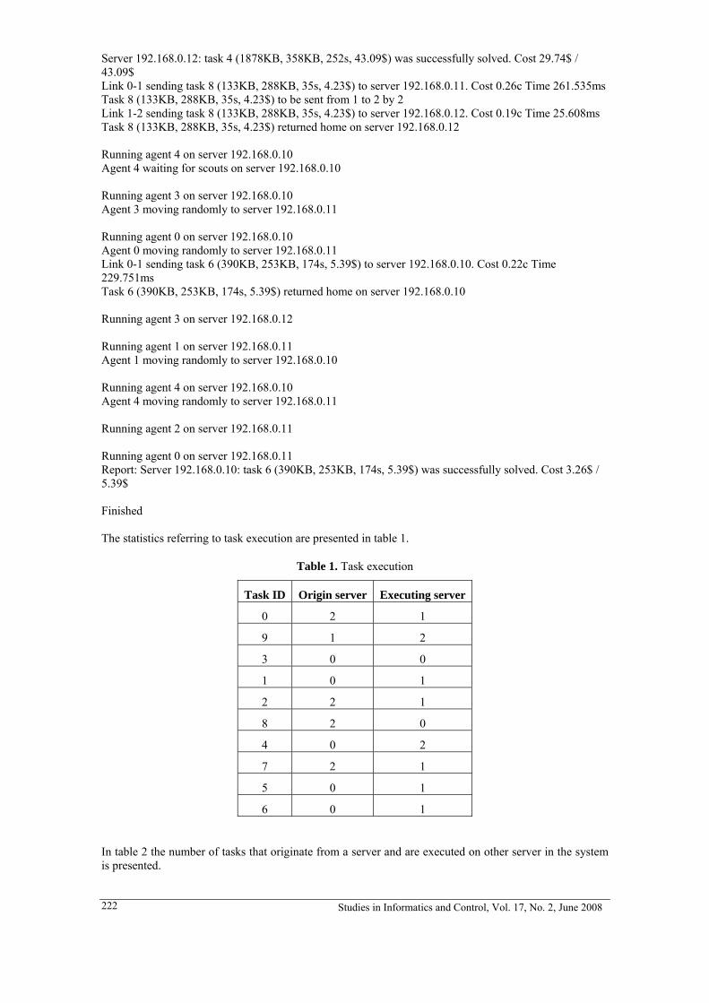
Server 192.168.0.12: task 4 (1878KB, 358KB, 252s, 43.09$) was successfully solved. Cost 29.74$ / 43.09$ Link 0-1 sending task 8 (133KB, 288KB, 35s, 4.23$) to server 192.168.0.11. Cost 0.26c Time 261.535ms Task 8 (133KB, 288KB, 35s, 4.23$) to be sent from 1 to 2 by 2 Link 1-2 sending task 8 (133KB, 288KB, 35s, 4.23$) to server 192.168.0.12. Cost 0.19c Time 25.608ms Task 8 (133KB, 288KB, 35s, 4.23$) returned home on server 192.168.0.12 Running agent 4 on server 192.168.0.10 Agent 4 waiting for scouts on server 192.168.0.10 Running agent 3 on server 192.168.0.10 Agent 3 moving randomly to server 192.168.0.11 Running agent 0 on server 192.168.0.10 Agent 0 moving randomly to server 192.168.0.11 Link 0-1 sending task 6 (390KB, 253KB, 174s, 5.39$) to server 192.168.0.10. Cost 0.22c Time 229.751ms Task 6 (390KB, 253KB, 174s, 5.39$) returned home on server 192.168.0.10 Running agent 3 on server 192.168.0.12 Running agent 1 on server 192.168.0.11 Agent 1 moving randomly to server 192.168.0.10 Running agent 4 on server 192.168.0.10 Agent 4 moving randomly to server 192.168.0.11 Running agent 2 on server 192.168.0.11 Running agent 0 on server 192.168.0.11 Report: Server 192.168.0.10: task 6 (390KB, 253KB, 174s, 5.39$) was successfully solved. Cost 3.26$ / 5.39$ Finished The statistics referring to task execution are presented in table 1.
Table 1. Task execution
Task ID Origin server Executing server
0 2 1
9 1 2
3 0 0
1 0 1
2 2 1
8 2 0
4 0 2
7 2 1
5 0 1
6 0 1
In table 2 the number of tasks that originate from a server and are executed on other server in the system is presented.
Studies in Informatics and Control, Vol. 17, No. 2, June 2008 222
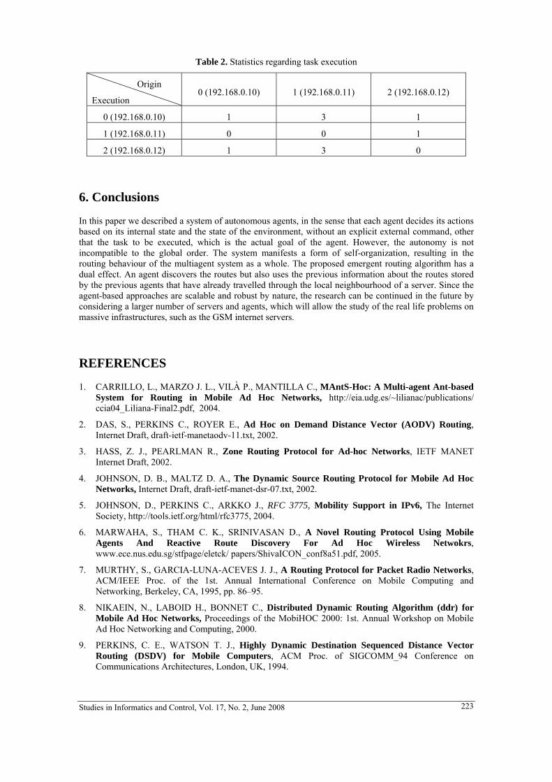
Table 2. Statistics regarding task execution
Origin
Execution 0 (192.168.0.10) 1 (192.168.0.11) 2 (192.168.0.12)
0 (192.168.0.10) 1 3 1
1 (192.168.0.11) 0 0 1
2 (192.168.0.12) 1 3 0
6. Conclusions
In this paper we described a system of autonomous agents, in the sense that each agent decides its actions based on its internal state and the state of the environment, without an explicit external command, other that the task to be executed, which is the actual goal of the agent. However, the autonomy is not incompatible to the global order. The system manifests a form of self-organization, resulting in the routing behaviour of the multiagent system as a whole. The proposed emergent routing algorithm has a dual effect. An agent discovers the routes but also uses the previous information about the routes stored by the previous agents that have already travelled through the local neighbourhood of a server. Since the agent-based approaches are scalable and robust by nature, the research can be continued in the future by considering a larger number of servers and agents, which will allow the study of the real life problems on massive infrastructures, such as the GSM internet servers.
REFERENCES
1. CARRILLO, L., MARZO J. L., VILÀ P., MANTILLA C., MAntS-Hoc: A Multi-agent Ant-based System for Routing in Mobile Ad Hoc Networks, http://eia.udg.es/~lilianac/publications/ ccia04_Liliana-Final2.pdf, 2004.
2. DAS, S., PERKINS C., ROYER E., Ad Hoc on Demand Distance Vector (AODV) Routing, Internet Draft, draft-ietf-manetaodv-11.txt, 2002.
3. HASS, Z. J., PEARLMAN R., Zone Routing Protocol for Ad-hoc Networks, IETF MANET Internet Draft, 2002.
4. JOHNSON, D. B., MALTZ D. A., The Dynamic Source Routing Protocol for Mobile Ad Hoc Networks, Internet Draft, draft-ietf-manet-dsr-07.txt, 2002.
5. JOHNSON, D., PERKINS C., ARKKO J., RFC 3775, Mobility Support in IPv6, The Internet Society, http://tools.ietf.org/html/rfc3775, 2004.
6. MARWAHA, S., THAM C. K., SRINIVASAN D., A Novel Routing Protocol Using Mobile Agents And Reactive Route Discovery For Ad Hoc Wireless Netwokrs, www.ece.nus.edu.sg/stfpage/eletck/ papers/ShivaICON_conf8a51.pdf, 2005.
7. MURTHY, S., GARCIA-LUNA-ACEVES J. J., A Routing Protocol for Packet Radio Networks, ACM/IEEE Proc. of the 1st. Annual International Conference on Mobile Computing and Networking, Berkeley, CA, 1995, pp. 86–95.
8. NIKAEIN, N., LABOID H., BONNET C., Distributed Dynamic Routing Algorithm (ddr) for Mobile Ad Hoc Networks, Proceedings of the MobiHOC 2000: 1st. Annual Workshop on Mobile Ad Hoc Networking and Computing, 2000.
9. PERKINS, C. E., WATSON T. J., Highly Dynamic Destination Sequenced Distance Vector Routing (DSDV) for Mobile Computers, ACM Proc. of SIGCOMM_94 Conference on Communications Architectures, London, UK, 1994.
Studies in Informatics and Control, Vol. 17, No. 2, June 2008 223

10. PERKINS, C., RFC 3344, IP Mobility Support for IPv4, The Internet Society, http://tools.ietf.org/html/rfc3344, 2002.
11. WOOLDRIDGE, M., Intelligent Agents, in G. Weiß (ed.), Multiagent Systems - A Modern Approach to Distributed Artificial Intelligence, The MIT Press, Cambridge, Massachusetts, 2000.
12. WOOLDRIDGE, M., JENNINGS N. R., Intelligent Agents: Theory and Practice, The Knowledge Engineering Review, Vol. 10(2), 1995, pp. 115-152.
13. ZAHARIA, M. H., LEON F., System Prototype for the Dynamic Management of Distributed Resources in Mobile Computing Using Intelligent Agents, CNCSIS project code 66/2005, Technical Report, 2006.
14. ZAHARIA, M. H., LEON F., CALISTRU C. N., GÂLEA D., Load Balancing in Heterogeneous Distributed Systems Using Mobile Intelligent Agents, IEEE International Conference on Distributed Human-Machine Sysems, Athens, Greece, 2008.
Studies in Informatics and Control, Vol. 17, No. 2, June 2008 224

Decision Making Process: A Collaborative Perspective Pascale Zaraté
Université de Toulouse, INPT-IRIT
118 route de Narbonne, 31062 Toulouse Cedex 9, France
Abstract: The introduction of Information and Communication Technologies (ICT) in organisations implies an evolution of the decision making processes. This evolution is analysed on a cognitive and organisational point of view. These processes are analysed and described. The necessity to cooperate is then shown and we finally underline the fact that new systems must be designed in order to support the decision making process.
Keywords: Decision Making, Decision Support Systems, Cooperative Decision Support Systems.
Pascale Zaraté is an assistant professor at Toulouse University (INPT). She conducts her research projects at the IRIT laboratory (http://www.irit.fr). She holds a PhD in Computer Sciences / Decision Support from the LAMSADE laboratory at the Paris Dauphine University, Paris (1991). She also holds a Master degree in Computer Science from the Paul Sabatier University, Toulouse, France (1986); as well as a Bachelors degree Toulouse, France (1982). Pascale Zaraté’s current research interests include: distributed and asynchronous decision making processes; knowledge modelisation; cooperative knowledge based systems; cooperative decision making. Since 2000, she has been head of the Euro Working Group on DSS (www.euro-online.org). Since she obtained her PhD degree, she has edited a book, 9 special issues in several international journals and 4 proceedings of workshops. She published 29 papers, 10 of them in scientific international journals such as Journal of Decision Systems, Group Decision and Negotiation, EJOR. She has been elected expert review for the LACCIR foundation and the Science Academy of Czech Republic. In 2000 she was Co-President of the program committee of the COOP2002 conference. She is a member of the Scientific Committee of two International Journals: Journal of Decision Systems, ComSIS, Intelligent Decision Technologies and is associated editor of the Decision Support Systems Technology Journal. She is chairing the IFIP TC8/WG8.3 conference devoted to Collaborative Decision Making.
1. Introduction
[1] has shown that the Information and Communication Technologies (ICT) introduction in organisations obligatory leads to a time fragmentation. He also shows that the information overload is both a source and a consequence of this overload.
Nevertheless, with the great development of the ICT, the Decision Support Systems become partially usable: only when the decision makers meet each other. The collaborative work among several actors involved in a decisional process is reinforced. It becomes then essential to model the cooperation for the collaborative work.
Due to the economic evolution, the decisional processes in organisations present a great evolution. The reactivity obligation for companies and the technological evolution face the consequences that the cognitive and organisational decisional processes have been considerably modified.
2. Organisational Decision Making Process
The organisational decisional processes evolve and more actors participate to the decision: the responsibility and the initiative are more distributed.
On the other side, it is more and more necessary to have a report of activities. A great part of the managers’ activity aims to imply, motivate a great number of actors concerned by the problem to solve.
Even when the decision is organisationally made by one person, it is rather always prepared by a collaborative work. The cooperative processes increase and contribute more and more to decisions to make. Two fundamental conditions of the cooperation are facilitated by this evolution:
- The interactions are intensified, then the possibilities to establish cooperative behaviours increase and these cooperative behaviours effectively increase (see [2]; [3]).
- This exchange increase leads to better know the other actors’ objectives, which also are a preponderant issue to establish a cooperative behaviour (see [4]).
The organisational context is very present for decision making. It is fully part of the individual decisions through the actor involvement but also of the collective decisions. The organisational decisions by definition build up the organisation and at the same time determine its action. In other words, the decision making is often diffuse in the organisational and collaborative activity. The decision is
Studies in Informatics and Control, Vol. 17, No. 2, June 2008 225
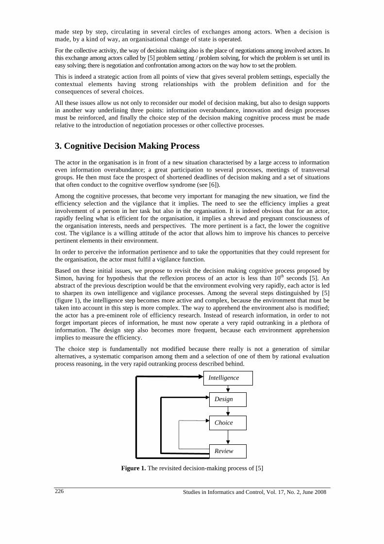
made step by step, circulating in several circles of exchanges among actors. When a decision is made, by a kind of way, an organisational change of state is operated.
For the collective activity, the way of decision making also is the place of negotiations among involved actors. In this exchange among actors called by [5] problem setting / problem solving, for which the problem is set until its easy solving; there is negotiation and confrontation among actors on the way how to set the problem.
This is indeed a strategic action from all points of view that gives several problem settings, especially the contextual elements having strong relationships with the problem definition and for the consequences of several choices.
All these issues allow us not only to reconsider our model of decision making, but also to design supports in another way underlining three points: information overabundance, innovation and design processes must be reinforced, and finally the choice step of the decision making cognitive process must be made relative to the introduction of negotiation processes or other collective processes.
3. Cognitive Decision Making Process
The actor in the organisation is in front of a new situation characterised by a large access to information even information overabundance; a great participation to several processes, meetings of transversal groups. He then must face the prospect of shortened deadlines of decision making and a set of situations that often conduct to the cognitive overflow syndrome (see [6]).
Among the cognitive processes, that become very important for managing the new situation, we find the efficiency selection and the vigilance that it implies. The need to see the efficiency implies a great involvement of a person in her task but also in the organisation. It is indeed obvious that for an actor, rapidly feeling what is efficient for the organisation, it implies a shrewd and pregnant consciousness of the organisation interests, needs and perspectives. The more pertinent is a fact, the lower the cognitive cost. The vigilance is a willing attitude of the actor that allows him to improve his chances to perceive pertinent elements in their environment.
In order to perceive the information pertinence and to take the opportunities that they could represent for the organisation, the actor must fulfil a vigilance function.
Based on these initial issues, we propose to revisit the decision making cognitive process proposed by Simon, having for hypothesis that the reflexion process of an actor is less than 10th seconds [5]. An abstract of the previous description would be that the environment evolving very rapidly, each actor is led to sharpen its own intelligence and vigilance processes. Among the several steps distinguished by [5] (figure 1), the intelligence step becomes more active and complex, because the environment that must be taken into account in this step is more complex. The way to apprehend the environment also is modified; the actor has a pre-eminent role of efficiency research. Instead of research information, in order to not forget important pieces of information, he must now operate a very rapid outranking in a plethora of information. The design step also becomes more frequent, because each environment apprehension implies to measure the efficiency.
The choice step is fundamentally not modified because there really is not a generation of similar alternatives, a systematic comparison among them and a selection of one of them by rational evaluation process reasoning, in the very rapid outranking process described behind.
Intelligence Design Choice Review
Figure 1. The revisited decision-making process of [5]
Studies in Informatics and Control, Vol. 17, No. 2, June 2008 226

The cognitive iterative process of decision making is then modified (figure 1): the two first steps are more often visited that the third one, the return loop from the choice to the intelligence, but also from the design to the intelligence are reinforced. Several iterations are necessary before the choice step (for more details on this process see [7]).
The evolution of the organisational and cognitive processes are strongly connected and operate in a simultaneously, causal and imbricate way.
4. Cooperation Necessity
In organisations, the great majority of decisions are made after an intensive consultation of several actors but not by individual decision makers working in larger organisations (see [8]). [8] have shown that the more complex organisations are, the less decisions are made by individual actors. For [9] the decision making processes in organisations generally imply several actors interacting each others. This interaction implies the information communication and a shared understanding by decision makers involved in these processes. They analyse this interaction along three issues: the used knowledge meaning must be common to every one; an artificial or not agent must have the necessarily authority for regulating the workloads; then the users must have enough confidence in the used technologies, that eventually could be seen through several visualisations of shared knowledge.
The participants to a decision making process must join their efforts in order to have a common goal where they must integrate multiple points of view not necessarily in harmony each others. They must work together not necessarily at the same place and at the same time. They are engaged in a coordination effort in order to solve the problem for which they must divide the decision making in several sub-tasks which will be assigned to individual participants.
5. Groups’ Evolution
Several authors analysed the collective decisional process along several issues without really introduce the context notion to take into account in the design of tools able to support the decision makers. We noticed that these analyses are established in several communities and more particularly those of the social psychology. In this last field, [10] has shown that the group behaviour is difficult to establish a generic analyse. The work context also must be taken into account. He also shows that it is necessarily to understand the nature of the task assigned to the group and its characteristics.
[11] analyses the collective decisional process under five dimensions: the group structure, the group roles, the group processes, the group style and the group norms. This analysis is for us interesting because it proposes a definition of the context of the group work.
The group structure is defined by several structures linked to the number of persons and the type of the group: individual, team with a hierarchy notion, and committee with a necessity of consensus among the group members, group less structured.
The group roles are assigned to one or several persons. Each member of the group can play one or several roles, which are easy to implement in a Decision Support Systems (user, analyst…).
The group processes used for the decision making could considerably influence it. If the information or decision making flows circulating are generally well-known, and could be analysed as workflows for example; the way how the process must emerge is generally not explicit et it could influence the decision in one or in another way. Must a consensus be raised? If yes, is there a deadline?
The group style is composed by the decision makers’ styles that could influence the process, its behaviour under several conditions and the decision making outputs quality.
The group norms are certainly the most important dimension. The social psychology of the decision making is in that sense very important.
It is necessary to be careful to use a common sense among participants; towards the collective or individual social pressures; towards the gender (balance male, female) and to the prescriptions about the group behaviour, the personal believes, the potential sanctions that constitute the decision making environment.
Following [12] the shared knowledge building among the group members dynamically arises and is strongly connected to a context proceduralisation, which is an activation of a general context part of
Studies in Informatics and Control, Vol. 17, No. 2, June 2008 227

the task implemented by interactions among individuals. Otherwise [13] defined a different context granularity from the decision making or task focus. He shows that the decision making context is dynamic and changes in accordance with the point of view adopted for the group observation: the group in itself or several individuals or the project context.
[13] published a case study on the publication of daily and weekly periodicals in Ireland. They have shown that the Information and Communication Technology (ICT) introduction in this enterprise has considerably modified the production process improving the enterprise effectiveness.
We analysed this case study through the five dimensions defined by [11].
The group structure is more diffuse, the group is generally constituted in an ad hoc way without a real formalisation of its structure. The group doesn’t know if it is structured as a team, a committee or in a hierarchical way.
The group style includes several styles coming from several groups constituting the decision making group; the group established only for a precise need, the members have not enough time for establishing a new style to the group. The group style is generally built through a long period.
The norms and the processes of the group become from several different groups and are then mixed one to each others.
The group roles include several roles coming from different groups, a group member will then create his own role that could be a mixed of several roles played in the past in other groups.
In other words, we could assume that the context dynamic of decision making influenced by the introduction of ICT is more reactive and volatile. The cognitive load of decision makers is more important because they share more information and they must remember more information (for more details see [14]).
6. New Supports: Cooperative Decision Support Systems
In order to support in a proper way this decisional process, new tools have to be designed. These systems are generally defined by several authors as frameworks integrating several tools. The main point of these frameworks is that the system must be able to support dynamically decision-makers by proposing an “Intelligent” assignment of tasks among the involved actors: decision-makers and software seen as agents.
[15] has shown that Cooperative Decision Support Systems must be developed. She defined these tools as frameworks composed by several tools. Therefore, we propose a Cooperative Decision Support framework. This framework is composed by several packages:
1. an interpersonal communication management system,
2. a task management system,
3. a knowledge management tool,
4. a dynamical man/machine interactions management tool (for more details see [15]).
7. Conclusion
According to [16] electronic communication has some effects on the group behaviour and she concludes by:
- An electronic meeting can be used as an ante-meeting to gather information and solicit opinions before a decision to be made face-to-face;
- Face-to-face decision making probably is the best when a decision requires complex thinking and subtle multiparty negotiations, and when problems are ill-defined (p. 191).
[17] concludes his study by assuming that: the study of the effectiveness of decision making could be studied, in order to highlight that too much technologies could generate negative effects, in particular the decline of consensus and personal participants implication.
Studies in Informatics and Control, Vol. 17, No. 2, June 2008 228
All these effects led us to think that a methodology of Collective DSS use has also to be defined. [17] concludes his study by assuming that face to face meeting must be planned during all along the group work, with a sufficient number, by using classical synchronous electronic meeting systems.
We are convinced by the fact that meeting points have to be introduced all along the group decision making process. This process has to be managed as a classical project and methodologies coming from project management domain could also be used. The meeting points have the same utility than the milestones in project management and offer the advantages of the face to face situation.
Our perspective of this work is to develop a methodology of Management for Collective Decision Making Processes supported by Cooperative Decision Support Systems.
REFERENCES
1. TETARD, F., Managers, Fragmentation of Working Time, and Information Systems, Thèse de doctorat de l’Université Abo Akademi, Turku, Finlande, 2002.
2. AXELROD, R., Donnant, donnant, Odile Jacob, Paris, 1992.
3. DELAHAYE, J.P., L’altruisme récompensé?, Pour la science, Paris, 1995.
4. ZACHARY, W. W. and ROBERSTON, S. P., Introduction, In Zachary W. W., Roberston S. P, Black J. B. Cognition, Computing and Cooperation. Ablex Publishing Corporation, Norwood, 1990.
5. SIMON, H., The New science of management decision, Prentice hall, Englewood-Cliffs, 1977.
6. TEULIER-BOURGINE, R. and ZARATE, P., : Vers une problématique de l’aide à la décision utilisant les connaissances. Actes de la Conférence en Ingénierie des Connaissances IC’01, Grenoble, France, 2001, pp. 147-166.
7. LAHLOU, S., Les attracteurs cognitifs et le syndrome du débordement, Intellectica 2000/1 no. 30, 2000, pp. 75-115.
8. GORRY, G. and SCOTT MORTON, M., A framework for management information systems, Sloan Management Review, volume 13 number 1, 1971, pp. 50-70.
9. SMOLIAR, S. and SPRAGUE, R., Communication and Understanding for Decision Support, Proceedings of the International Conference IFIP TC8/WG8.3, Cork, Ireland, 2002, pp. 107-119.
10. MAC GRATH, J. E., Groups - Interaction and Performance, (1st Edition), Prentice-Hall, Englewood Cliffs, N.J, 1984.
11. MARAKAS, G., Decision Support Systems In the 21st Century, Second Edition, Prentice Hall, 2003.
12. BREZILLON, P. Context dynamic and explanation in contextual graphs, In Blackburn P., Ghidini C., Turner R.M. and Giunchiglia F. (Eds.) Modeling and Using Context (CONTEXT-03), LNAI 2680, Springer Verlag Verlag, 2003, pp. 94-106.
13. BREZILLON, P., ADAM, F. and POMEROL, J.C., Supporting complex decision making processes in organizations with collaborative applications - A case study, In Favela J. and Decouchant D. (Eds.) Groupware: Design, Implementation, and Use, LNCS 2806, Springer Verlag, 2003, pp. 261-276.
Studies in Informatics and Control, Vol. 17, No. 2, June 2008 229

14. BREZILLON, P. and ZARATE, P. Group Decision Making: A Context oriented view, Proceedings of teh International Conference IFIP8/WG8.3, Meredith R., Shanks G., Arnott D., Carlsson S. (Eds), Prato, Italie, ISBN 0 7326 2269, 1-3 Juillet, 2004, pp. 123-133.
15. ZARATE, P., Cooperative Decision Support Systems, In Encyclopedia of Decision Making and Decision Support Technologies, Adam F. and Humphreys P. (Eds) IGI Global publication, 2008 (in press).
16. KIESLER, S., Group Decision Making and Communication Technology, Organizational Behaviour and Human Decision Processes, 52, 1992, pp. 96-123.
17. FAVIER, M., Performances des décisions de groupe assistées par un collecticiel : groupes en face à face versus groupes distribués, Revue Systèmes d’Information et Management, no. 3, 1996, 1996, pp.29-55.
Studies in Informatics and Control, Vol. 17, No. 2, June 2008 230

Computational Environment Generation for Computer Algebra Systems
Svetlana Cojocaru
Institute of Mathematics and Computer Science, Academy of Sciences of Moldova
Str. Academiei, 5, Chişinău, MD 2028, Republic of Moldova
Abstract: This paper deals with the problem of user interface development for Computer Algebra Systems. An algorithm of computational environment generation based on inferences from users’s actions is proposed.
Keywords: intelligent interface, computer algebra systems, adaptation
Svetlana Cojocaru – Dr. h., is the deputy director of the Institute of Mathematics and Computer Science, Academy of Science of Moldova. S. Cojocaru has published 3 books, 5 chapters in books, more than 100 papers. Her research interests include natural language processing, computer algebra, biological computing.
1. Introduction
The software complexity is permanently increasing and it requires from the user more vast and deep knowledge about systems functioning. Interfaces, which realize the human-computer interaction, take upon themselves to itself also a part of user’s tasks. But in the process of interface developing one can observe the same tendency as in general software evolution – they also become more and more complicated and insufficiently flexible. A solution of this problem might be intelligent interfaces, which are able to adapt themselves on user’s necessities, can learn, can take over the initiative in their interaction with user, are able to guide him in order to facilitate his objectives achieving in a fast and comfortable way.
Interface elaboration for Computer Algebra Systems (CAS) was and remains a topic to be investigated. There are a number of overviews treating this subject, among them we can mention (Kajler 1998, Kajler, Soiffer, 1998, Grabmeier, Kaltofen, Weispfenning, 2003). There is also a large list of concrete CAS descriptions, the corresponding interface (in a rudimentary or developed form) being one of the presented components.
Analysing the CAS interfaces one can conclude that they respect the requests specific for intelligent interfaces (Ross, 2000, Filip, 2007, Waern, 1997) in a reduced measure only:
• The user is guided in the process of his problem solution,
• It is not necessary to study preliminarily how the system works, often it is possible to learn the functioning mode directly in the process of interaction with the system,
• The system makes some errors prevention (partially) by checking the problem’s formulation correctness and verification of initial data.
Less significant is the attention paid to user modelling. Because CAS are from the very beginning oriented on a pre-established users class, their model (in relation to the class of problems, data type, non-ambiguous interpreting) is beforehand included into the system.
Therefore in the case of CAS it would be more relevant to speak about user’s personalisation. We should mention that the problem of personalisation, being realised, is not sufficiently examined. User can apply some possibilities of individualisation, but he should adapt the system to his needs or preferences by himself.
We will note also that the possibility to interact in natural language in the frame of CAS is rather limited.
Thus, in order to increase the intelligence level of CAS interfaces one can fix the necessity to implement some additional features, including user’s personalisation, adaptation to his individual requests and preferences. One should note, that the user not always is able to formulate his preferences.
Studies in Informatics and Control, Vol. 17, No. 2, June 2008 231

In the next sections the process of adaptation in CAS interfaces will be examined. We will respect the following principles:
• The goal of adaptive systems is to facilitate user’s objectives achieving in the fastest and easiest way, assuring, as much as possible, a high degree of satisfaction (Ross, 2000).
• It is important that system shall not irritate the user, not reduce by its interventions the speed of his work, it shall not initiate unbidden operations in some inappropriate moments, creating in such a way obstacles to achieve the goal immediately.
2. Adaptation to the User
The more widely is used a software product the more difficult is to elaborate a comfortable environment, which will be able to assure a high performance for every user. A series of studies performed since 1980 had been finished in conviction that there is no possibility to specify all varieties of users, programs and equipment in order to work out interfaces ideally convenient for each case. The only resource comparable with the number of users are the users themselves, therefore namely they should be involved in the process of the personalised interfaces developing (Weld, Anderson, Domingos, 2003).
Analysis of many CAS interfaces convinced us that even in the case of the most developed ones users have some wishes, which demand an adaptation to their interests and individual habits (Cojocaru, Malahova, Colesnicov, 2006). As it was mentioned above, adaptation to user is one of the distinctive, indispensable features of intelligent interfaces. We will describe the process of its implementation in general case and the specific for CAS in particular.
Let us recall that the adaptation process might be realised in the following three modes:
• Adaptation is performed in advance, by a design oriented to a specific type of users.
• The system permits a dynamic adaptation, which is performed by user in the process of his interaction with the system.
• The adaptation is made by system in the process of its interaction with the user.
In the last case the adaptation is made through a dialogue initiated by the system or through “spying” user’s actions and making adjustments to his preferences basing on inferences from the collected knowledge.
In some sense we can consider that all CAS are from the very beginning oriented on a fixed class of problems and a determined group of users, thus the last two methods of adaptation will be the subject of our interest. The case, when the system permits a dynamic adaptation realised according to user’s request (and with his contribution) is frequently implemented in modern software and is called “customization”. In (Weld, Anderson, Domingos, 2003) the following ways of implementing of that adaptation method are underlined:
• Visible menu selection,
• Adding buttons in menu bar,
• Definition of macros,
• Using specialised programming languages to write own scripts.
Of course, only a limited number of users poses the necessary abilities and have sufficient time (and patience) to apply this methods (especially, the last two), therefore, keeping in mind all these possibilities, we will deal with dynamic adaptation initiated by the system. Our approach will be explained basing on the example of Computer Algebra system Bergman (www.servus.math.su.se/bergman).
3. Interface of Computer Algebra System Bergman
Bergman is a computer algebra system calculating non-commutative and commutative Gröbner basis, Hilbert series, Anick's resolution, and Betti numbers for ideals over rings and for modules. Bergman allows a multitude of choices for various kinds of input, operation, output, etc. One may let predefined
Studies in Informatics and Control, Vol. 17, No. 2, June 2008 232

“top of the top'” procedures make the choices for him, or specify details by means of a large number of lower level mode setting procedures.
To perform some computations in Bergman you should set up the polynomial ring and its surrounding. This action includes selection of the algebra type (commutative or non-commutative), the variables, the ordering, the characteristic, type of coefficients, and variable weights. One can also select the strategy of computation, and input-output mode. There are some minor mode selections too. For a complete description see (Backelin, Cojocaru, Ufnarovski, 2005).
Note, that different kinds of calculations demand different parameters settings, they should be compatible with each other and compatible with the corresponding calculation procedure. Because Bergman has a high degree of flexibility in modes selection, sometimes it might be difficult for user to make a correct and efficient selection. These problems are avoided by developing of graphical user interface, which permits to operate with Bergman in a manner close to the usual mathematical surroundings.
The main principles respected in the process of interface design correspond both to common requests and to those specific for intelligent interfaces, namely:
• the interface reflects specific mathematical object and notions,
• it is possible to use the system without preliminary studying of its description,
• some tasks are taken over from the user and executed by the system,
• the interface simplifies access to different Bergman’s functions,
• the interface operates the data control before calculations,
• input and output can be performed in bi-dimensional format,
• it is possible to save the environment in which the computations were performed and to repeat the calculations in the same conditions, with the same or modified data.
Moreover, the interface can serve also as a prospectus for Bergman giving the possibility to see on the graphical panel the most important facilities without reading a manual or applying the corresponding help function.
The shell consists of the main menu at its top, then the toolbar, and then three panels (top-left, bottom-left, and the right one). The main menu consists of items that are used to organize calculations, and the top-left panel contains drop-down menus and other elements that specify mathematical parameters of the problem to be solved. The bottom-left and right panels display information, or are used to enter some data (e.g., variables and relations are input from the right panel). Main menu items are those ordinary (File, Tools, Options, Windows, Run etc.), but there are two specific ones named Sessions and Environment. These items are less obvious and we shall explain them.
Our observations on CAS using permit to conclude that most of the mathematicians deal for a more or less long period with research of a certain class of problems, which need calculations in a specific mathematical environment, determined by a series of parameters. These parameters remain mostly unchanged during several computation sessions, only a few of them may be modified (for example, in the case of Bergman many calculations are performed only by variations related to input polynomials or modules). We introduced the notion of Environment just to establish this repeatable surrounding. It fixes the preferable setup immediately after starting Bergman. It is possible to have a number of environments for each user, depending on the class of problems one is interested to solve. Moreover, it is possible to make some changes in the environment, permanent or valid during the current session. The same environment might be used by different users if they solve the problems belonging to the same class.
A possibility with a higher degree of determinism is that realized by the mechanism of sessions. A session is a set of parameters that fully defines the problem to be solved. Session is implemented as a directory where all data are saved, Bergman input files are generated, and Bergman output files are produced. Sessions serve to return to previous Bergman calculations, modify them, and experiment with them. Informally, sessions give to a mathematician the possibility to use the previous experience of Bergman's users (own or others) and to save the current setup for the future calculations.
When the user wants to create a new session, he will be asked which environment should be used as the
Studies in Informatics and Control, Vol. 17, No. 2, June 2008 233
base to create this session. An environment is a partial set of data common for several sessions. It corresponds to the group of mathematical problems the user investigates during different sessions. E.g., after Bergman’s installation the environment directory contains a profile called ``commutative'' that fixes a single parameter, the commutativity. There is also a pre-defined environment containing the default settings. For example, by default, if no other settings are made, Bergman will calculate Gröbner basis in the commutative ring with characteristics equal to zero.
4. Environment Generation
The menu items Environment and Session serve to implement the mechanism of adaptation. There are three methods implementing environment creation in Bergman.
The first one is based on a dialogue operated by the system. It puts a number of questions, collecting and analyzing the answers so that it becomes possible to fix necessary data permitting to generate the computational environment. Each question is followed by a list of possible answers. A fragment of such a dialogue is presented below:
> (dialogue)
What kinds of objects do you plan to work with?
- One of the following: grc, ngrc, grnc, ngrnc
> grc
The suggested answers mean correspondingly "gradded commutative", "non-gradded commutative" etc. Obviously, this method can be used only by persons having some experience in work with the system.
The second method is based on session editing; it might be the current session or any of the saved ones. The system displays the list of parameters with corresponding values and proposes to select the wanted ones. The selected values can be edited if necessary.
The third method is based on inferences from user’s actions. The series of previously saved sessions are analyzed and on their base a new environment is created. In adaptation based on inferences, as a rule, one of two possible criteria is used: that of recent actions or that of frequent actions (Gajos et al., 2006). We propose an heuristic algorithm which will take in account both criteria. It is necessary to mention that solving of this problem for CAS has its peculiarities: the parameters’ values, selected from different sessions according to the frequency criterion might be contradictory.
Let be a sequence of attributes associated with Computer Algebra System . Each attribute
has a corresponding set of values nAA ,,1 K S
iA },,{ 1 ikii vvV K= ),,1;,,1( rkni KK == . These values form a multidimensional array
],,,[],,,[],,,[ 212222111211 21 mmnmmnnS vvvXvvvXvvvF KKKK= .
The element has the value 1 if there exists a sequence of values the attributes
can have in system , otherwise miiif K21 miii vvv ,,,
21K
mAAA ,,, 21 K S 02
=mi iiif K . This array will be called a compatibility
function.
Basing on these attributes and values we construct the corteges
.,,1)},(,),{( , NlvAvACsj msjsjjmjl KK == ++
Each cortege will have the corresponding weight . lt
Our aim is to construct a cortege C following both criteria of the most frequent and most recent actions
Studies in Informatics and Control, Vol. 17, No. 2, June 2008 234
adding one by one attributes with compatible values. Initially we will take into account the frequency criterion. Let
iAϕ be the initial threshold of frequency.
1. An attribute A is included into cortege C if it is present at least in ϕ of corteges . lC
2. The value v of this attribute is established equal to the most frequent value of the attribute A occurred in corteges . If there are two or more values with equal frequencies go to step 3, if not – go to step 4.
lC
3. Use the recent action criterion: among the values with equal (maximal) frequencies select as a value of attribute A that, which belongs to the cortege with the greatest weight.
4. Verify if values from the obtained cortege satisfy the compatibility function. If yes, then C is the result, else go to step 5.
5. From the sequence of values select that component (or those components) which cause the incompatibility. Replace them with other values having lower frequencies. Repeat step 4 if such values exist, otherwise go to step 6.
6. It was not possible to construct a cortege with those parameters. Replace them, namely the sequence of initial corteges , the threshold of frequency lC ϕ . Repeat the process starting with step 1.
The proposed algorithm does not produce always a resulting cortege. In an unsuccessful case on can vary the initial parameters (the sequence of corteges , the threshold of frequency lC ϕ etc.) and repeat the process until a result satisfying the compatibility function will be obtained.
5. Conclusions
N. Kajler (Kajler, 1998) considers computer-human interaction in symbolic computation “a wide and interdisciplinary research area”, including different aspects, which “current user interfaces either do not handle well or do not address at all”. We tried to cover only a small part of them, namely the problem of adaptation to users using the mechanism of computational environments and sessions. Our experience shows that in many cases about 5 saved sessions are enough to be able to understand user’s preferences and to generate for him a convenient environment reflecting his domain of interests.
REFERENCES
1. BACKELIN, J., S.COJOCARU, V.UFNAROVSKI, Mathematical Computations Using Bergman, Lund University, Centre for Mathematical Science, 2005, 206 p.
2. COJOCARU, S., L. MALAHOVA, A. COLESNICOV, Providing Modern Software Environments to Computer Algebra Systems, Computer Algebra in Scientific Computing, Proceedings of the 9th International Workshop, CASC 2006, Chişinău, Moldova, September 11-15, 2006. LNCS, Springer, pp. 120-140.
3. COJOCARU, S., A. COLESNICOV, L. MALAHOVA, Interfaces to Symbolic Computation Systems: Reconsidering Experience of Bergman, Computer Science Journal of Moldova, ISSN 1561-4042, Vol. 13, No. 2, 2005, pp. 232-244.
4. FILIP, F. G., Decision Support Systems, Editura Tehnică, Bucureşti, 2007, 364 p. (in Romanian).
5. GAJOS, K., M. CZERWINSKI, D. TAN, D. WELD, Exploring the Design Space for Adaptive Graphical User Interfaces, In: Proceedings of the working conference on Advanced visual interfaces - 2006, Venezia, Italy, May 23 - 26, 2006, pp. 201 – 208.
6. GRABMEIER, J., E. KALTOFEN, V. WEISPFENING (eds.) Computer Algebra Handbook, Springer, 2003, 637 p.
Studies in Informatics and Control, Vol. 17, No. 2, June 2008 235

7. N. KAJLER (ed.). Computer-Human Interaction in Symbolic Computation, Springer-Verlag, Wien, 1998, 212 p.
8. KAJLER, N., N. SOIFFER, A Survey of User Interfaces for Computer Algebra Systems, Journal of Symbolic Computation, Vol. 25, issue 2, February 1998, pp. 127-159.
9. ROSS, E., Intelligent User Interfaces: Survey and Research Directions, Technical report, CSTR-00-004, March, 2000, Department of Computer Science, University of Bristol (www.cs.bris.ac.uk/Publications/Papers/1000447.pdf)
10. WAERN, A., What is an Intelligent Interface? Available at www.sics.se/˜annika/papers/intint.html
11. WELD, D., C. ANDERSON, P. DOMONGOS et al., Automatically Personalizing User Interfaces, In: Proceedings of IJCAI-03, 2003, Acapulco, Mexico, available at www.cs.washington.edu/homes/weld/papers/weld-ijcai03.pdf.
Studies in Informatics and Control, Vol. 17, No. 2, June 2008 236

Editorial
Large-scale complex systems (LSS) have been traditionally represented in control literature by models which are characterized by a large number of state and control variables, strong nonlinearities and uncertainties. Their decomposition into smaller, more manageable subsystems, possibly organized in a hierarchy, has been associated with intense and time-critical information exchange and with the need for efficient decentralization and co-ordination mechanisms.
The last decade of the past Millennium and the early years of the 21st century have revealed new characteristic features of industrial and non-industrial large-scale and complex systems. The enterprise of the present time is to operate in a highly networked environment. Also there is an ever more increased concern for new aspects such as: a) integration of various technologies, b) economic, environmental, and social aspects, and c) security issues. Consequently, the design of control systems must take into account more aspects and needs additional skills and tools. At the same time, the recent advances in computer and communication technologies have shown that they can provide effective tools and adequate technical infrastructures to support the design and enable the implementation of advanced control systems for the large-scale and complex applications of the present time.
The TC (Technical Committee) 5.4 on "Large-Scale Complex Systems" of IFAC (International Federation of Automatic Control) has already a more than 30-year tradition. The main events of this TC are the symposia entitled "Large- Scale Systems: Theory and Applications". The inaugural edition was held in Udine, Italy in 1976. Since then, at a three-year succession, the Symposium took place in Toulouse, France (1980), Warsaw, Poland (1983), Zurich, Switzerland (1986), Berlin, GDR (1989), Beijing, China (1992), London, UK (1995), Patras, Greece (1998), Bucharest, Romania (2001), Osaka, Japan (2004), and Gdansk, Poland ( 2007). The next edition of Symposium will be held in Lille, France, in 2010.
In 2002, at the IFAC World Congress and General Assembly held in Barcelona , the IFAC Technical Committee 5.4 was placed under the Coordinating Committee "Manufacturing and Logistic Systems", chaired by Professor Shimon Nof. Since then, the scope and objectives of the TC have been adapted accordingly to reflect the current trends in control systems and the new place of this TC within the IFAC organization. The TC focuses on manufacturing and related systems which are characterized by complexity and/or a networked structure of interconnected subsystems. It aims at developing new decentralized and hierarchical control methods, decision-making, and risk analysis techniques together with practical solutions based on new advances in computer and communication tools. A practical consequence of the new place of the TC is organizing the MCPL (Management and Control of Production and Logistics) conference starting with 2004. MCPL conferences were held in Santiago de Chile (2004) and Sibiu, Romania (2007). The next MCPL conference is to be organized in Coimbra, Portugal in 2010.
It can be appreciated now that several subfields that are traditional for LSS domain remain of increasing interest to the scientific community, such as decentralized and hierarchical control, model reduction, optimization, and complex system analysis. Traditional applications of LSS methods, such as power, gas, transportation, manufacturing, environmental systems are more than ever of great interest. The new issues such as collaborative control, intelligent network systems, risk management and decision support in LSS are well received by the LSS community. Among main ideas and trends one can include: a) large systems become ever “larger” (more complicated and networked) and b) there is still a need for practical solutions, possibly including new technologies with a view to attaining a correct balance between control techniques and computer and communication tools.
At the LSS symposium in Gdansk a formal meeting of the TC5.4 was held and Prof. Brdys of Birmingham University, UK, was elected for nomination as a chair of the Committee. According to Prof. Brdys, complexity is anticipated to be a central problem in modern system theory and practice. Complexity issues in control of large scale and complex systems such as manufacturing systems and related systems require a deeper and systematic continuation in the development of a relevant theory of complex systems including its extension to recent communication issues. Variety of theoretic results motivated by practice and successfully developed within various long term activities of this TC could offer a deep background for such continuation. Multidisciplinary approaches appear to be adequate in modelling and controlling large-scale and complex systems
At the end of my second term as a chair of the TC 5.4, I intended to publish a special issue of this journal addressing several relevant aspects and results in LSS domain. Consequently, the present issue of the

journal contains several papers of the members of the TC and other invited authors.
Wan, Ruan, and Liu of China review their investigating efforts and results over the past fifteen years in the on-line steady-state hierarchical intelligent control and optimization of large-scale industrial processes, a research direction initially proposed by Roberts three decades ago. Borowa and colleagues from UK and Poland describe an approach for detecting and localisation of pipe leakage in Drinking Water Distribution Systems (DWDS) which are large-scale and complex distributed dynamic systems. A practical DWDS is decomposed into suitable subnetworks which make the monitoring process easier while fewer sensors are required. The subnetworks and corresponding PCA ( Principal Component Analysis) monitoring models are selected based on the network operational knowledge and information regarding its topology. Duviella, Chiron and Charbonnaud of France propose a weighted digraph representation of dam-river systems to solve the water asset-management by resource allocation and setpoint assignment problem. Tangour and Borne of EC Lille ( France ) give a review of several various metaheuristics optimisation methods which have been implemented in various applications such as the optimization manufacturing problems and recommend hybrid approaches. Chamroo and colleagues from France and Bulgaria propose a new control scheme for a highly non-linear anaerobic digestion process. Ivanescu and Florescu of Romania present a solution for the control problem of a hyperredundant robot with continuum elements that performs the coli function for grasping. Ayadi and his colleagues from Tunisia propose a practical approach to design and implement a real-time system based on a RISC microcontroller dedicated to a DC motor speed control.
Leon, Zaharia, and Galea of Romania propose a system of autonomous agents for dynamic routing in high performance distributed systems.
Pascale Zarate of France presents several methodological issues in an effort to develop Cooperative Decision Support Systems (CDSS) for collective decision making processes. In order to make the information systems more usable, Svetlana Cojocaru from the Moldavian Academy of Sciences propose intelligent interfaces, which are able to adapt themselves to user’s learning needs, take over the initiative in their interaction with user, are able to guide him so that the objectives may be achieved in a fast and comfortable way.
F. G. Filip
Chair, IFAC TC 5.4 (2002-2008)

AUTHOR INDEX Ayadi, M., 201
Benrejeb, M., 201
Borne, P., 169
Borowa, A., 135
Bouallègue, S. 201
Brdys, M. A., 135
Chamroo, A., 181
Charbonnaud, P., 153
Chiron, P., 153
Christov, N., 181
Cojocaru, S., 231
Duviella, E., 153
Duzinkiewicz, K., 135
Florescu, M. C., 189
Gâlea, D., 215
Grochowski, M., 135
Haggège, J., 201
Ivanescu, M., 189
Jezior, K., 135
Leon, F., 215
Liu, D., 123
Mazur, K., 135
Popescu, D., 189
Popescu, N., 189
Ruan, X.-E., 123
Simeonov, I., 181
Tangour, F., 169
Vasseur, C., 181
Wan, B.-W., 123
Zaharia, M. H., 215
Zaraté, P., 225


I N S T R U C T I O N S T O A U T H O R S
SIC welcomes original contributions on all aspects of research and practice in IT. Authors should not submit to SIC material that is under consideration elsewhere. Papers should preferably not exceed 15 standard typewritten pages. However, while concision improves chances of publication, serious consideration will be given to articles in which the nature and quality of the content justify greater length. Articles should be sent if possible in disk form, accompanied by two printouts and a cover letter signed by the (principal) author to the following address: National Institute for R&D in Informatics, Publishing Department, 8-10 Averescu Blvd., Bucharest 011455 Romania
The manuscript should be arranged in the following order: title; author's name and forename; name and address of the organization authors belong to; abstract; keywords and phrases; short biographical notes, main body of the paper; references in alphabetical order by first author's surname; tables and figures. Headings should be numbered by Arabic numbers. Tables and figures should be titled, numbered consecutively, put on separate white sheets. Legends are to be typewritten on a separate page. References in the text must have in the order of their occurrence a consecutive number included in brackets. For references, quotations etc., please follow the conventions used in recent issues of SIC. (http://www.ici.ro/ici/revista/sic.html)
We always acknowledge receipt of contributions submitted to us. After a preliminary triage to eliminate submissions that are unsuitable for the SIC journal, the remaining science-based papers, will enter a review process which typically takes 4-6 weeks from the time we acknowledge the receipt of the paper. Following the confirmation to the corresponding author of acceptance for publication of the submitted article (presumably sent as a hard copy), a quick editing and printing work would be possible if agreed to provide a soft copy, on diskette or via e-mail, under Windows (Microsoft Word 2003).
It is a condition of publication in SIC that authors grant an exclusive licence to the Journal, which is operated on the Journal's behalf by the Publisher, by completing a copyright licence form. This ensures that requests from third parties to reproduce articles are handled efficiently and consistently and will also allow the article to be as widely disseminated as possible. When an article is published, a PDF of the final version is emailed to the corresponding author. It is the author's responsibility to obtain permission to reproduce verbal or visual material from copyright sources.
